Quantum computing quantum Monte Carlo with hybrid tensor network for electronic structure calculations

Abstract

Quantum computing quantum Monte Carlo (QC-QMC) is an algorithm that can be combined with quantum algorithms such as variational quantum eigensolver (VQE) to obtain the ground state with higher accuracy than either VQE or QMC alone. Here we propose an algorithm combining QC-QMC with hybrid tensor network (HTN) to extend the applicability of QC-QMC for the system beyond the size of a single quantum device, called HTN+QMC. For HTN in a two-layer quantum-quantum tree tensor, HTN+QMC for an $\order{n^{2}}$-qubit trial wave function can be executed by using only a $n$-qubit device excluding ancilla qubits. Our algorithm is evaluated on the Heisenberg chain model, the graphite-based Hubbard model, the hydrogen plane model, and MonoArylBiImidazole using full configuration interaction QMC. We found that the algorithm can achieve energy accuracy several orders of magnitude higher than VQE or QMC, and HTN+QMC gives the same energy accuracy as QC-QMC when the system is appropriately decomposed. Moreover, we develop a pseudo-Hadamard test technique that enables efficient overlap calculations between a trial wave function and a standard basis state. In a real device experiment using the technique, we obtained almost the same accuracy as the statevector simulator, indicating the noise robustness of HTN+QMC.

I Introduction

Computationally accurate prediction of physical properties enables us to speed up the development of functional materials such as batteries [Ceder1998-re, Gao2021-hr], catalysis [Norskov2009-fr], and photochemical materials [Turro1991-qw, Michl1990-pn]. The physical properties are mainly governed by electrons in materials, and the computational cost of calculating electronic structures increases exponentially with system size in general, which often prevents classical computers from achieving the required accuracy to predict the properties.

Quantum computers are expected to solve such classically intractable problems in quantum chemistry and materials science [Bauer2020-ug]. Current quantum computers are called noisy intermediate scale-quantum (NISQ) devices [Preskill2018-sc], which have limitations on the numbers of both qubits and quantum gates due to physical noise, and various approaches for the NISQ devices are proposed [Bharti2022-ov, Cerezo2021-dy]. One of the most popular algorithms is the variational quantum eigensolver (VQE) [Peruzzo2014-kp] which is used to obtain the ground state energy by minimizing energy cost function using a variational quantum circuit, where its parameters are updated by a classical computer. In contrast to the traditional quantum algorithms such as the quantum phase estimation [Yu_Kitaev1995-cf], VQE requires much smaller hardware resources. However, VQE still suffers from many issues such as insufficient accuracy [Stilck_Franca2021-qx] and vanishing parameter gradients so-called barren plateau [McClean2018-pn].

In addition to the studies to avoid those issues [Grant2019-fv, Skolik2021-ju, Cerezo2021-kj, Kanno2023-ip], there are multiple variants of quantum Monte Carlo (QMC), which were proposed for further relaxing the hardware requirement [Huggins2022-ly, Yang2021-ie, Tan2022-fh, Xu2023-sn, Zhang2022-lf, Layden2023-ke, Lee2022-lq]. QMC is a computational method that uses stochastic sampling techniques to solve large quantum many-body problems such as molecular systems containing hundreds of electrons [Austin2012-qi, Al-Hamdani2021-ns]. To date, various types of QMC approaches have been proposed including variational Monte Carlo [McMillan1965-dd, Ceperley1977-yz], auxiliary field quantum Monte Carlo [Blankenbecler1981-is, Sugiyama1986-xm], and full configuration interaction quantum Monte Carlo (FCIQMC) [Booth2009-lv], where we adopt FCIQMC in this study. In FCIQMC, which is useful for quantum chemistry, a stochastic imaginary-time evolution is executed in the space of all the standard basis states (such as the Slater determinants) that can be constructed from a given spatial orbital basis. As in Refs. [Huggins2022-ly, Xu2023-sn, Zhang2022-lf], a type of QMC called quantum computing QMC (QC-QMC) was introduced. Combined with a quantum algorithm such as VQE, QC-QMC is used to improve the accuracy of energy evaluation in ground-state calculations by mitigating the sign problem, which otherwise causes an exponential statistical error in the energy evaluation [Troyer2005-bk]. Specifically, the wave function distribution, i.e., the walker distribution, is classically generated, and energy is evaluated by using a trial wave function prepared by VQE. In contrast to VQE where the accuracy depends on parameter optimization, QC-QMC has no such optimization while the accuracy relies on the quality of the trial wave function in the energy evaluation. The ground state computation without optimization is expected to lower the hardware requirements, and in fact, there was a demonstration on a 16 qubit diamond, the largest hardware experiment run nearly within the chemical accuracy [Huggins2022-ly].

While QC-QMC is expected to provide highly accurate ground-state calculations, applying this method to large-scale systems is one of the remaining challenges. Although the electronic correlations outside the active space can be obtained by classical post-processing [Huggins2022-ly], the size of the available active space is limited by that of the trial wave function. The proposals for constructing wave functions larger than the size of a quantum device include the divide-and-conquer algorithm [Yamazaki2018-pu, Fujii2022-bq], embedding theory [Kawashima2021-os, Greene-Diniz2022-xo, Cao2022-hn], circuit cutting [Peng2020-xc, Harada2023-ym], perturbation [Sun2022-bh], and tensor network [Huggins2019-qa, Yuan2021-ih]. Hybrid tensor network (HTN) [Yuan2021-ih] is a general framework of the tensor network that can be implemented on a reduced number of qubits and gates by decomposing the wave function in the original system into smaller-sized tensors, and these tensors are processed by either quantum or classical computation, i.e., quantum/classical hybrid computation. Such a decomposition can reduce both the effective width and depth of the circuit, which is more robust to noise than the original circuit. There are several quantum algorithms or ansatze depending on the tensor network structure, which include the matrix product states [Schollwock2011-im], projected entangled pair states [Verstraete2004-lj], and tree tensor networks (TN) [Shi2006-he, Huggins2019-qa]. In the two-layer TN, which is adopted in this study, the quantum states of the subsystem in the first layer are integrated with the second layer either by a quantum or classical method. We refer to the former and latter types as quantum-quantum TN (QQTN) and quantum-classical TN, where the deep VQE [Fujii2022-bq] and entanglement forging [Eddins2022-ny, Motta2022-oz] can be broadly classified into the quantum-quantum and quantum-classical ones, respectively. If gaining the quantum advantage (rather than noise robustness) is a priority, QQTN is preferred.

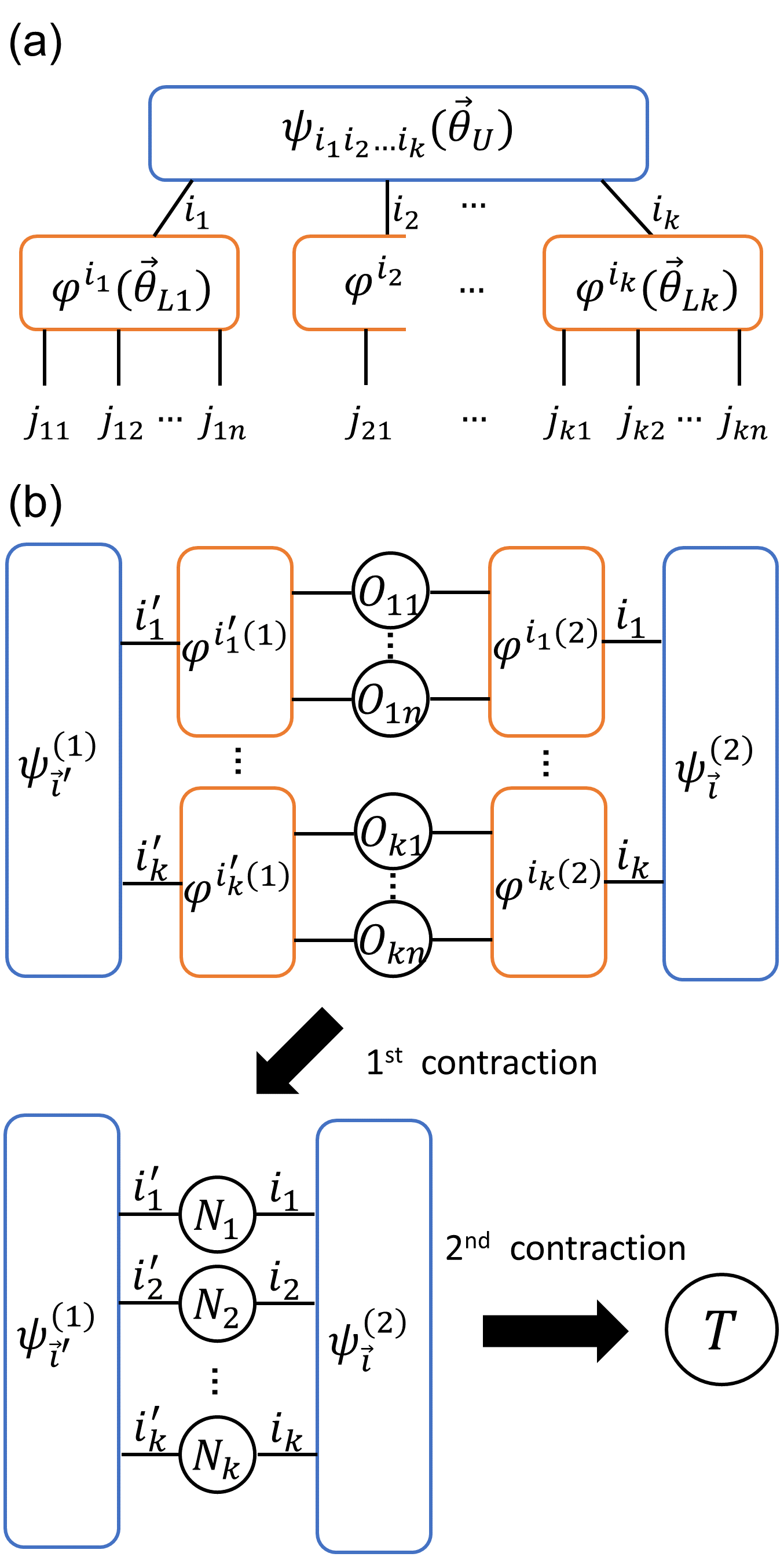
Figure 1: Representation and calculation of hybrid tensor network in the two-layer QQTN. (a) The hybrid tensor network representation of the two-layered QQTN state. (b) The calculation of $T$ in Eq. (2), where we omit the parameters. See Sec. IV.3 for details.

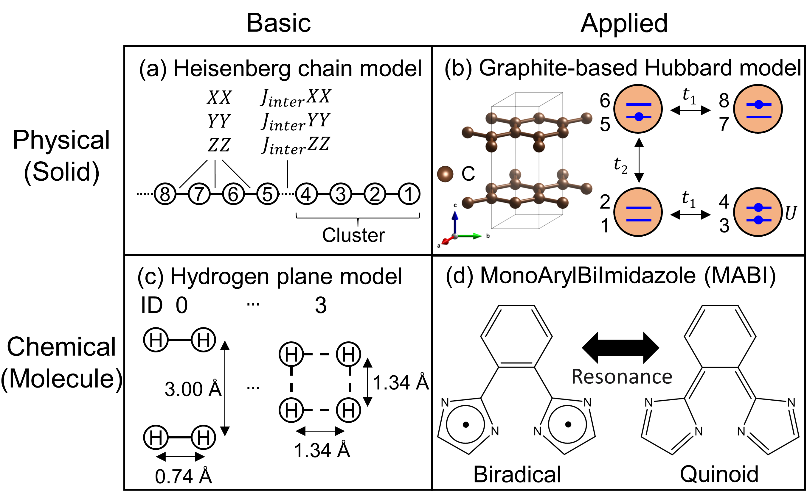
Figure 2: Models for benchmarking HTN+QMC. The structure of graphite is drawn by VESTA [Momma2011-ck]. The qubit indices are labeled in (a) and (b), see Sec. II.1 for details. (a) The Heisenberg chain model. (b) The graphite-based Hubbard model. (c) The hydrogen plane model. (d) MonoArylBilmidazole (MABI).

In this study, we propose an algorithm of QC-QMC in combination with HTN of a two-layered QQTN. In particular, we consider the following QQTN:

$$\ket{\psi_{HTN}(\vec{\theta}_{HTN})}$$ (1)

$$=\sum_{\vec{i}}\psi_{\vec{i}}(\vec{\theta}_{U})\left(\prod_{m=1}^{k}\varphi^{i_{m}}(\vec{\theta}_{Lm})\right)\left(\bigotimes_{m=1}^{k}\ket{\vec{j}_{m}}\right)$$

$$=\sum_{\vec{i}}\psi_{\vec{i}}(\vec{\theta}_{U})\bigotimes_{m=1}^{k}\ket{\varphi^{i_{m}}(\vec{\theta}_{Lm})}.$$

The tensor network representation of this state is depicted in Fig. 1(a). The tensors $\psi_{\vec{i}}(\vec{\theta}_{U})$ ($\varphi^{i_{m}}(\vec{\theta}_{Lm})$) are defined using wave functions $\ket*{\psi(\vec{\theta}_{U})}$ ($\ket*{\varphi^{i_{m}}(\vec{\theta}_{Lm})}$) as $\psi_{\vec{i}}(\vec{\theta}_{U})=\innerproduct*{\vec{i}}{\psi(\vec{\theta}_{U})}$ ($\innerproduct*{\vec{j}_{m}}{\varphi^{i_{m}}(\vec{\theta}_{Lm})}$), where $\vec{i}=i_{1}i_{2}\dots i_{k}$ ($\vec{j}_{m}=j_{m1}j_{m2}\dots j_{mn}$) being a $k$ ($n$)-qubit binary string. $\psi_{\vec{i}}(\vec{\theta}_{U})$ and $\varphi^{i_{m}}(\vec{\theta}_{Lm})$ are assumed to be constructed by quantum circuits, where $\vec{\theta}_{U}$ and $\vec{\theta}_{Lm}$ are variational parameters of the upper tensor (blue), and the $m$-th lower tensor (orange), respectively. The detail of the algorithm is given in Sec. IV (and Appendices A, B, and C), where calculating the transition amplitude between a pair of the wave functions $T(\vec{\theta}_{HTN}^{(1)},\vec{\theta}_{HTN}^{(2)})$ is a major part:

$$T(\vec{\theta}_{HTN}^{(1)},\vec{\theta}_{HTN}^{(2)})=\matrixelement{\psi_{HTN}^{(1)}(\vec{\theta}_{HTN}^{(1)})}{O}{\psi_{HTN}^{(2)}(\vec{\theta}_{HTN}^{(2)})},$$ (2)

where the observable $O$ is defined using tensor products $O=\bigotimes_{m,r}O_{mr}$, and $O_{mr}$ is an observable attached on the $r$-th qubit of the $m$-th subsystem $(r=1,2,\dots,n)$. As shown in Fig. 1(b), the transition amplitude $T(\vec{\theta}_{HTN}^{(1)},\vec{\theta}_{HTN}^{(2)})$ is calculated by first performing a quantum computation on the lower tensor, classically processing the obtained results to generate the contracted operators $N_{m}$, and then contracting them again with a quantum computation on the upper tensor. Here, the specific expressions of Eq. (2) when performing the algorithm are

$$\matrixelement{\psi_{HTN}(\vec{\theta}_{HTN})}{O}{\psi_{HTN}(\vec{\theta}_{HTN})},$$ (3)

and

$$\innerproduct{\psi_{HTN}(\vec{\theta}_{HTN})}{\phi_{h}},$$ (4)

where $\ket{\phi_{h}}$ is the ${h}$-th standard basis state as in a Slater determinant, and $O$ is implicitly included in Eq. (4) as $O=I^{\otimes nk}$. The HTN+QMC algorithm consists of two steps; we first optimize $\vec{\theta}_{HTN}=(\vec{\theta}_{U},\vec{\theta}_{Lm})$ to prepare the trial wave function, by calculating Eq. (3). In the second step, we execute QMC by using the trial wave function $\ket{\psi_{HTN}(\vec{\theta}_{HTN})}$, which was optimized in the first step, and Eq. (4). We will denote HTN+VQE when referring to the first step only and omit the parameter in $\ket{\psi_{HTN}}$ hereafter. In this formalism, thanks to the contraction technique shown in Fig. 1(b), when $k\sim n$, we can construct $\order{n^{2}}$-qubit trial wave function in QMC by using only $n$-qubit device excluding ancilla qubits.

We benchmarked the performance of HTN+QMC for the Heisenberg chain model, the hydrogen ($\mathrm{H_{4}}$) plane model, the graphite-based Hubbard model, and MonoArylBiImidazole (MABI), which are classified into four material categories: physical or chemical (solid or molecule) and basic or applied as in Fig. 2. The first two models are commonly used as the benchmark [Motta2019-sf, Huggins2022-ly], Graphite is a two-dimensional layered material and is used as an anode material for lithium-ion batteries [Thinius2014-xz], and MABI is a model system of the photochromic radical dimer PentaArylBiImidazole (PABI) [Kobayashi2017-ty]. We also execute HTN+QMC on a real device $ibmq\_kolkata$ by the newly developed algorithm to calculate the overlap between the trial wave function and the standard basis state required in HTN+QMC. We call this algorithm a pseudo-Hadamard test because the Hadamard test type circuit is used in the algorithm. We mention that the proposed algorithm can be applied to other types of HTN structures and QMC, and the overlap technique can be extended to calculate a transition amplitude between two wave functions.

II Results

II.1 Benchmarking models

The performance of HTN+QMC is benchmarked with the Heisenberg chain model, the graphite-based Hubbard model, the hydrogen plane model, and MABI. The Heisenberg chain model, as shown in Fig. 2(a), is defined as a chain of $k$ clusters consisting of four sites

$$H =\sum_{p=1}^{k}H_{p}+J_{inter}\sum_{p^{\prime}=1}^{k-1}H_{p^{\prime}},$$ (5)

where

$$H_{p} =\sum_{f=1}^{3}X_{4(p-1)+f}X_{4(p-1)+f+1}$$ (6)

$$+Y_{4(p-1)+f}Y_{4(p-1)+f+1}$$

$$+Z_{4(p-1)+f}Z_{4(p-1)+f+1},$$

$$H_{p^{\prime}} =X_{4p^{\prime}}X_{4p^{\prime}+1}+Y_{4p^{\prime}}Y_{4p^{\prime}+1}+Z_{4p^{\prime}}Z_{4p^{\prime}+1}.$$ (7)

The intra- and inter-cluster interactions are 1 and $J_{inter}$, respectively. In the benchmark, we consider $k=2$ and $3$, i.e., 8- and 12-qubit models and $J_{inter}=0.2,0.4,\dots,2.0$ Hartree.

Figure  2(b) shows our graphite-based Hubbard model (the graphite model hereafter), where two layers of graphene sheets are modeled with periodically aligned unit cells, in which two carbon atoms reside in each layer. Using two qubits to represent the up and down spin orbitals ($p_{z}$ orbitals) in each carbon atom, we define the Hamiltonian with 8 qubits as

$$H =3t_{1}\sum_{q=1,2,5,6}(a_{q+2}^{\dagger}a_{q}+a_{q}^{\dagger}a_{q+2})$$ (8)

$$+2t_{2}\sum_{q=1,2}(a_{q+4}^{\dagger}a_{q}+a_{q}^{\dagger}a_{q+4})$$

$$+U\sum_{q=1,3,5,7}n_{q+1}n_{q},$$

where $q$ is the spin-orbital index for the $p_{z}$ orbital in the carbon, and $q=1,2,3$ and $4$ ($5,6,7$ and $8$) corresponds to the first (second) layer. $a_{q}^{\dagger}$ ($a_{q}$) is the creation (annihilation) operators on the $q$-th site, and $n_{q}$ is the number operator $n_{q}=a_{q}^{{\dagger}}a_{q}$. $t_{1}$ and $t_{2}$ are the hopping energy between the first and second nearest neighbor sites corresponding to the intra- and inter-layer interaction energy, respectively, and $U$ is the on-site Coulomb energy. The prefactors for $t_{1}$ and $t_{2}$ are due to periodic boundary conditions, e.g., the prefactor for $t_{2}$ is 2 because two inter-layer interactions exist per carbon (one inside the unit cell and the other outside the unit cell). The reason for $t_{2}$ being only on two indices, $q=1$ and 2, is that graphite is AB stacking. We determine the value of $t_{1}$, $t_{2}$, and $U$ by the electronic structure calculation. For details see Appendix D.

The Hamiltonians for the hydrogen plane model (8-qubit model) in Fig. 2(c) and MABI (12-qubit model) in Fig. 2(d) were constructed using their restricted Hartree-Fock orbitals of their ground states as molecular orbital bases. In the hydrogen plane model, the two hydrogen molecules are arranged vertically as in the index (ID) 0 of Fig. 2(c). Then the intermolecular and intramolecular distances are shortened and lengthened, respectively, until the shape of the hydrogen plane becomes a square as in ID 3. The two structures are interpolated between ID 0 and 3, thus benchmarking a total of four structures.

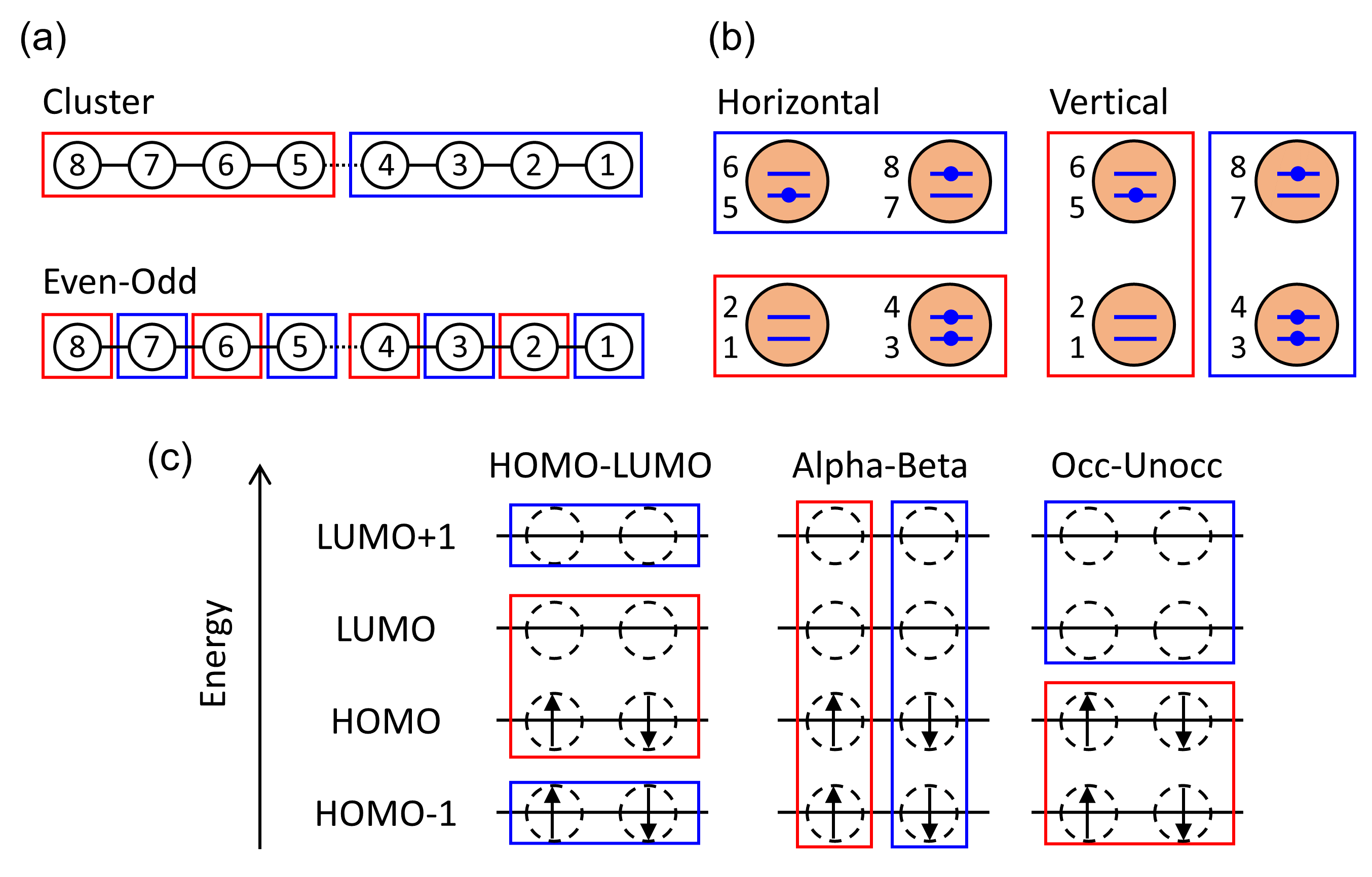
Figure 3: Decomposition settings. $n=4$ and $k=2$ are assumed for all the figures. (a) The settings for the Heisenberg chain model. (b) The settings for the graphite-based Hubbard model. (c) The settings for chemical models in the case of the eight-qubit model.

Next, we present the specific conditions for constructing the benchmarking models. The decomposition settings used for individual models are as follows; for the Heisenberg chain model, the cluster and even-odd settings refer to decomposing the model into subsystems by the cluster and even and odd indices, respectively, as illustrated in Fig. 3(a); for the graphite model, the horizontal and vertical settings refer to decomposing the model horizontally and vertically with respect to the sheet (in the ab-axis plane in Fig. 2(b)), respectively, as in Fig. 3(b); for the chemical models (hydrogen plane model and MABI), the HOMO-LUMO, alpha-beta, and occ-unocc settings refer to decomposing the model using the pair of HOMO$-x$ and LUMO$+x$ as units ($x=0$ and $1$ in the hydrogen plane model and $x=0,1$, and $2$ in MABI), based on alpha and beta spin-orbitals, and based on occupied and unoccupied orbitals, respectively, as in Fig. 3(c), where the orbitals of the chemical models are shown in Appendix D; the no-decomposition setting refers to the calculation without decomposing the original system, i.e., not using HTN. The cluster setting for the Heisenberg model, the horizontal setting for the graphite model, and the HOMO-LUMO setting for chemical models are adopted as a default.

Figure 4 shows the quantum circuit called real amplitude ansatz, a popular hardware efficient ansatz employed for devices with linear connectivity layout. Figure (a) shows an original circuit, which is used for the statevector, whereas, in order to run on real devices, a variant with ancilla qubit was considered as in figure (b), where details on the operation will be given in Sec. II.2.3. In both ansatze, the rotation angle of the RY gate (i.e., the parameter) is updated at the VQE and HTN+VQE iterations while in the second step of QC-QMC and HTN+QMC, it is fixed. Because HTN+VQE demands quite a high computational cost due to its iterative process, the real device ($ibmq\_kolkata$) was used only for the overlap calculation in the second step, i.e., not for HTN+VQE computations.

The depth represents the value for the real amplitude ansatze, which are $k$-qubit and $n$-qubit circuits for upper and lower tensors, respectively, in HTN, whereas $nk$-qubit circuits in the no-decomposition setting (in which ancilla qubit is not counted). Here, $k$ and $nk$ represent the number of subsystems and the number of system qubits, respectively. Thus, the numbers of parameters in the settings of HTN and the no-decomposition setting are different even with $d_{H}=d_{N}$, where the numbers in the statevector and real device procedure of HTN are the same when $d_{H}=\tilde{d}_{H}$. The numbers of parameters in the settings of HTN with $d_{H}$ and the no-decomposition setting with $d_{N}$ are $nk(d_{H}+1)+k(d_{H}+1)$ and $nk(d_{N}+1)$, respectively. We set $d_{H}=4$ as a default by referring to the benchmark results in Appendix F. The initial parameters for the VQE and HTN+VQE are chosen randomly from $[0,1)$ and $[0,2\pi)$ in the statevector and the real device procedure, respectively. Note that only the results that are specifically relevant to the discussion are described in the main text while the rest of the results are shown in the appendices.

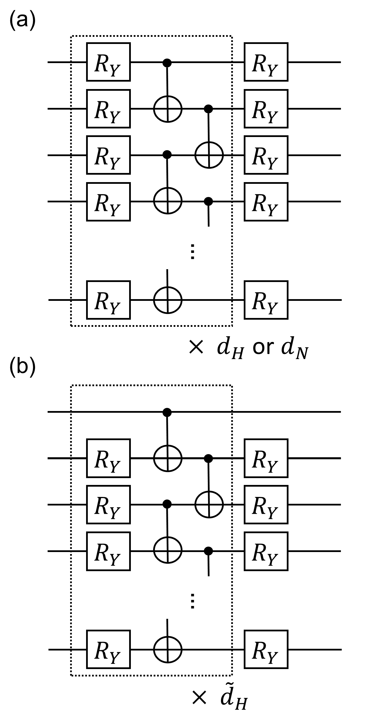
Figure 4: Circuits of real amplitude ansatz in this study. $d_{H}$, $d_{N}$, and $\tilde{d}_{H}$ are the depth in HTN, the no-decomposition setting, and HTN (real device), i.e., the block surrounded by the dotted line is repeated $d_{H}$ or $d_{N}$, and $\tilde{d}_{H}$ times, respectively. (a) The circuit in statevector procedure. All the lines represent system qubits. (b) The circuit in real device procedure. The topmost line represents an ancilla qubit and the other lines represent system qubits.

In all the QMC methods (QMC, QC-QMC, and HTN+QMC), we evaluate the mean and standard deviation of the (mixed) energy over 5,000 to 10,000 iterations. Hereafter (absolute) deviation from the exact ground state is referred to by energy difference. See Appendix E for the details of the conditions of VQE and QMC.

II.2 Numerical results

First, we demonstrate the performance improvements in HTN+QMC for HTN+VQE for the Heisenberg chain model, which is then followed by the analysis of all the benchmarking models. Then for the Heisenberg chain model, we discuss the HTN+QMC performance focusing on the dependencies on the decomposition settings. Finally, we describe the operational principle of the pseudo-Hadamard test technique and present the results of the real device experiments for the hydrogen plane model and MABI using that technique.

II.2.1 Performance improvements

Figure 5(a) shows the result of executing HTN+VQE for the Heisenberg chain model in the cluster setting with $d_{H}=4$, $k=2$, and $J_{inter}=1.0$ Hartree. As in the inset, the energy difference from the exact ground state energy is $4.4\times 10^{-1}$ Hartree at the end of the optimization. Figure 5(b) shows the result for HTN+QMC. In the HTN+QMC result, the energy difference from the exact value is $5.3\times 10^{-3}$ Hartree, which is an improvement by two orders of magnitude from the result for HTN+VQE. In addition, compared to the QMC result, the HTN+QMC results show higher accuracy and less energy fluctuation. Specifically, the energy differences (standard deviations) for QMC and HTN+QMC are $5.5\times 10^{-1}$ and $5.3\times 10^{-3}$ Hartree ($7.7\times 10^{-1}$ and $4.8\times 10^{-2}$ Hartree), respectively. Therefore, the energy accuracy would be improved in HTN+QMC compared to either HTN+VQE or QMC alone, and we will discuss the details of this improvement in the next subsection.

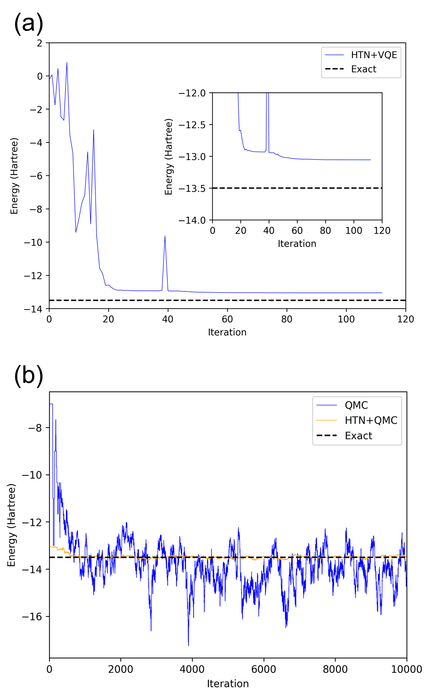
Figure 5: Results of the energy in the Heisenberg chain models of the cluster setting with $n=4$, $k=2$, $J_{inter}=1.0$, and $d_{H}=4$. The black dashed line represents the energy of the exact ground state. (a) The result for HTN+VQE (blue line). The inset is an enlarged view along the y-axis. (b) The results for QMC (blue line) and HTN+QMC (orange line).

Table 1: Energy differences in VQE, QMC, and HTN+QMC, and fidelity for HTN+VQE and the single reference state for the Heisenberg chain models of the cluster setting with $k=2$ and $3$ and $J_{inter}=1.0$, the graphite model of the horizontal setting with $k=2$, the hydrogen plane model of HOMO-LUMO setting with $k=2$ and ID 3, and MABI of HOMO-LUMO setting with $k=3$, where $n=4$ and $d_{H}=4$ for all the models. $\Delta$ in the table denotes the energy difference. The energy unit is Hartree.

Models	$\Delta$HTN+VQE	$\Delta$QMC	$\Delta$HTN+QMC	Fidelity (HTN+VQE)	Fidelity (single reference state)
Heisenberg chain ($k=2$)	$4.4\times 10^{-1}$	$5.5\times 10^{-1}$	$5.3\times 10^{-3}$	0.92	0.13
Heisenberg chain ($k=3$)	$1.0\times 10^{0}$	$3.5\times 10^{-1}$	$4.0\times 10^{-2}$	0.80	0.06
Graphite	$6.4\times 10^{-4}$	$4.6\times 10^{-4}$	$8.1\times 10^{-6}$	1.00	0.09
Hydrogen plane	$3.5\times 10^{-2}$	$9.1\times 10^{-4}$	$3.0\times 10^{-5}$	0.44	0.45
MABI	$2.4\times 10^{-2}$	$6.6\times 10^{-5}$	$9.2\times 10^{-6}$	0.94	0.86

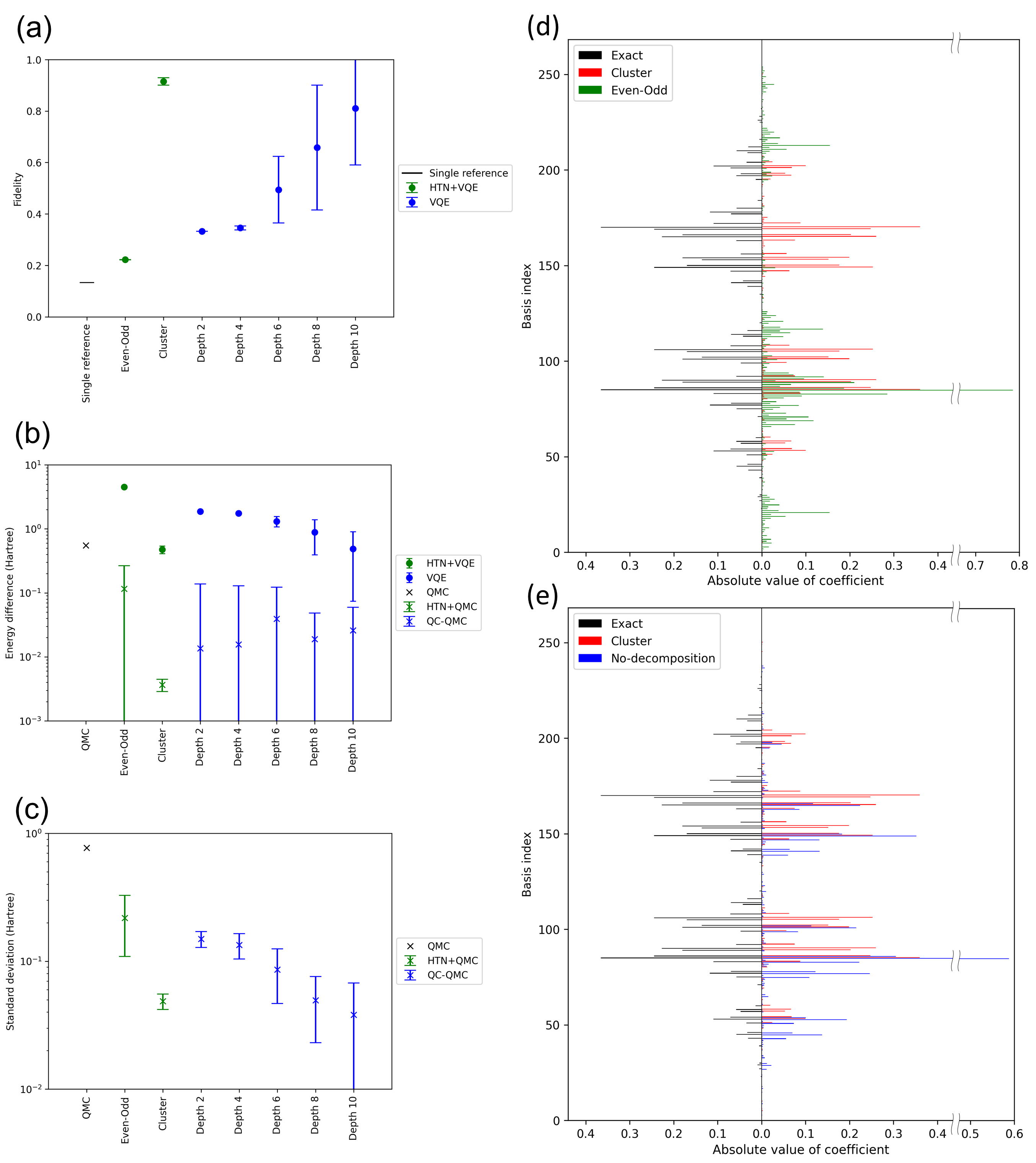
Figure 6: Results of the analysis for the Heisenberg chain model with $J_{inter}=1.0$. (a), (b), and (c) are the decomposition dependencies. The average and error bar is obtained over 10 different random seeds used for the initial parameters in VQE or HTN+VQE. The fidelity of the single reference state is plotted by the black bar in (a), and the energy difference and standard deviation by the black cross markers in (b) and (c), respectively. The green (blue) circle and cross markers denote the results for the decomposition (no-decomposition) setting in HTN+VQE and HTN+QMC (VQE and QC-QMC), respectively, with $d_{H}=4$ ($d_{N}=2,4,\dots,10$). In HTN+VQE and HTN+QMC, $n=4$ and $k=2$ for all the settings. (d) and (e) are the distributions of the wave function for the Heisenberg chain model with $J_{inter}=1.0$. The basis index is the value when the standard basis state is expressed in the decimal number, e.g., $\ket{10000010}$ corresponds to 130. The black, red, green, and blue bars represent the coefficients for the exact ground state, HTN+VQE result with the cluster setting, HTN+VQE result with the even-odd setting, and VQE result with the no-decomposition setting, respectively. (a) The fidelity. (b) The energy difference. (c) The standard deviation. (d) The comparison of the exact ground state, cluster setting, and even-odd setting. (e) The comparison of the exact ground state, cluster setting, and no-decomposition setting ($d_{N}=6$).

Here we briefly comment on the other models, for which the computational results are described in detail in Appendix F. Table 1 shows the results summarized on HTN of the Heisenberg chain models with $k=2$ and $3$, the graphite model, the hydrogen plane model with ID 3, and MABI. In all the models, the difference for HTN+QMC is one to several orders of magnitude smaller than that for either HTN+VQE or QMC alone. Especially for the hydrogen plane model, the difference for HTN+QMC is one order of magnitude smaller than that for QMC, even though the fidelity for HTN+VQE is 0.44, almost the same as that for the leading single standard basis state in the exact ground state (single reference state hereafter), 0.45. The above result indicates that the performance of QMC may be improved even if the trial wave function does not have high fidelity, and it is important to evaluate the quality of the trial wave function through the QMC computation.

II.2.2 Dependences on the decomposition settings

We consider the Heisenberg chain model with $k=2$, $n=4$, and $J_{inter}=1.0$, which was computed in the cluster, even-odd, and no-decomposition settings. Prior to the results, we introduce an average interaction strength between the subsystems $G_{mr}$ as a simple measure of decomposition defined as

$$G_{mr}=\frac{1}{k}\sum_{a}\absolutevalue{c_{a}}\delta_{amr},$$ (9)

where $\delta_{amr}=1$ if Pauli $X,Y$, or $Z$ operator is included in $\bigotimes_{r}P_{amr}$ of the Hamiltonian, which is defined in Sec. IV.4, in more than two subsystems, and $\delta_{amr}=0$ otherwise. $G_{mr}$ in the cluster setting and even-odd setting are 1.5 and 10.5 Hartree, respectively, i.e., the cluster setting seems to be suitable for the trial wave function preparation. In Appendix G, we also show the values of $G_{mr}$ for the graphite model, the hydrogen plane model with ID 3, and MABI, and we have confirmed that the results, especially in the physical models, are almost consistent with intuition. For example, in the graphite model, $G_{mr}$ of the horizontal setting has one order of magnitude smaller than that of the vertical setting. The chemical models especially in the hydrogen plane model, however, give results that differ from intuition, which indicates that more sophisticated measures might be needed in complicated systems. The mutual information, which represents the degree of dependence between random variables, could be used as the alternative measure [Zhang2020-vv, Zhang2022-mu]. We also show the values using the exact ground state in the appendix, which tends to be more consistent with intuition than $G_{mr}$. Although the exact ground states cannot be obtained in realistic situations, in a previous study [Zhang2020-vv], the classical construction of approximate value using the density matrix renormalization group (DMRG) is proposed.

Figure 6(a), (b), and (c) show the decomposition dependencies of the fidelity, the energy difference, and the standard deviation for the Heisenberg chain model. In cases of the decomposition settings, the fidelity (Fig. 6(a)) in the cluster setting 0.92 is four times higher than in the even-odd setting 0.22, as expected from the values of $G_{mr}$. We also calculated the bipartite entanglement entropy of the exact ground state when decomposing the cluster and even-odd, which is 0.66 and 3.46. It is evident that an appropriate choice of the decomposition setting is crucial in the performance of the trial wave function.

In addition, the fidelity for the cluster setting is equal to or slightly higher than that for the no-decomposition setting with $d_{N}=10$ whereas the fidelity for the even-odd setting is lower than for the no-decomposition setting with $d_{N}=2$. Here, the numbers of the parameters for the cluster setting with $d_{H}=4$ and the no-decomposition setting with $d_{N}=10$ are $nk(d_{H}+1)+k(d_{H}+1)=50$ and $nk(d_{N}+1)=88$, respectively. That is, the cluster setting with fewer parameters shows comparable performance to the no-decomposition setting. The increase in the fidelity is obviously related to the decrease in the energy difference in HTN+VQE and HTN+QMC as in Fig. 6(b), and that in the standard deviation in HTN+QMC as in Fig. 6(c). A similar tendency for the fidelity, energy difference, and standard deviation can be found in the graphite model, the hydrogen plane model, and MABI, see Appendix G for the details. From the results, we can expect that if the system is appropriately decomposed, i.e., if the interaction between the subsystems is small, HTN can prepare a trial wave function that performs as well as or better than the wave function generated by the quantum circuit of the original system size. Note that the fidelities for the hydrogen plane model with ID 3 are almost the same or lower than that of the single reference state depending on the decomposition settings as shown in Appendix G. One of the ways to increase the fidelity is an improvement of the initial wave function used in the VQE or HTN+VQE. As shown in the appendix, the fidelity can increase in some cases by using the initial state which is close to the Hartree-Fock state. In addition, while the parameters of all the tensors are sequentially optimized in this study, separate optimization of one tensor by another could be an alternative [Haghshenas2022-zn].

The high performance in the cluster setting seems to arise from that the wave function represented by the QQTN in Fig. 1(a) has a problem-inspired structure while the ansatz actually used for each tensor is hardware efficient one. In order to analyze the wave function in detail, we first compare the distribution of the absolute coefficient of the standard basis state, which was calculated by using one of the 10 random seeds in Fig. 6 (a), (b), and (c). As shown in Fig. 6(d), the cluster setting exhibits a distribution very close to that of the exact ground state, in comparison to the even-odd setting. Note that for the even-odd setting, the distribution was calculated with the basis state encoding, where the qubit index was reordered from $8,7,6,5/4,3,2,1$ to $8,6,4,2/7,5,3,1$ as shown in Even-Odd of Fig. 3(a). This qubit index was then changed back to that of Cluster in the plotting, allowing for direct comparison with the even-odd setting.

We then examine the wave function, which is represented as a linear combination of tensor products of the subsystems. In the case of the cluster setting for the Heisenberg chain model, we can approximately describe the exact ground state $\ket{\psi_{g-C}}$ by four dominant terms with respective coefficients of $c_{1}=-0.37,c_{2}=0.24,c_{3}=-0.23$, and $c_{4}=0.18$, as

$$\ket{\psi_{g-C}} \simeq c_{1}(\ket{\textbf{0101}}\otimes\ket{\textbf{0101}}+\ket{1010}\otimes\ket{1010})$$ (10)

$$+c_{2}(\ket{\textbf{0101}}\otimes\ket{\textbf{0110}}+\ket{1001}\otimes\ket{0101}$$

$$\quad+\ket{1010}\otimes\ket{1001}+\ket{0110}\otimes\ket{1010})$$

$$+c_{3}(\ket{\textbf{1010}}\otimes\ket{\textbf{0101}}+\ket{0101}\otimes\ket{1010})$$

$$+c_{4}(\ket{0101}\otimes\ket{1001}+\ket{0110}\otimes\ket{0101}$$

$$\quad+\ket{1001}\otimes\ket{1010}+\ket{\textbf{1010}}\otimes\ket{\textbf{0110}}).$$

The state is energetically favored because of the (sub)antiferromagnetic spin configurations, where there is at most one spin pair with the same parity (e.g., 00 and 11), considering that all terms in the Hamiltonian of Eqs. (5), (6), and (7) are positive. Each term consists of a primitive basis state (in bold) and the spin and spatial inverted ones, where the ground state redefined in this primitive basis $\{\ket{\textbf{0101}},\ket{\textbf{1010}}\}\otimes\{\ket{\textbf{0101}},\ket{\textbf{0110}}\}$ is regarded as a separable state (with the same number of up/down spins in each subsystem), which can be accurately prepared by the lower tensors with one leg connecting to the upper tensor. In case of the even-odd setting, where the qubit index is reordered and the number of up (or down) spins in the subsystem takes 0 to 4, the state in such a primitive basis, e.g., $\{\ket{\textbf{0000}}\otimes\ket{\textbf{1111}},\ket{\textbf{0001}}\otimes\ket{\textbf{1110}},\ket{\textbf{1100}}\otimes\ket{\textbf{0011}},\ket{\textbf{1101}}\otimes\ket{\textbf{0010}}\}$, is no longer separable, resulting in a lower fidelity than in the cluster setting. Through the above mechanism, the decomposition setting affects the fidelity, where matching between the tensor network state and the target state is a crucial factor, being in analogy with the discussion in the area low with tensor networks. Note that the number of legs limits the dimension of the basis for state preparation.

The HTN+VQE results with the cluster setting in Fig. 6(d) show that the coefficients for the above 12 basis states are of the same magnitude as $c_{1},c_{2},\dots,c_{4}$. In contrast, the even-odd setting gives a much less accurate wave function; half of the basis states in Eq. (10) was negligibly small in magnitude, and the coefficient of $\ket{0101}\otimes\ket{0101}$ is 0.78, which is so large leading to quite different distribution from the exact.

Next, Fig. 6(e) shows the distribution of the no-decomposition setting, where the distributions of the ground state and cluster settings are reproduced from the figure (a) for comparison. The depth is set to $d_{N}=6$ such that the numbers of parameters in the no-decomposition and cluster settings become comparable, that is, 50 and 48, respectively. The distribution for the no-decomposition setting deviates from that for the exact wave function, and half of the basis states in Eq. (10) were negligibly small in magnitude. In general, the no-decomposition setting would achieve higher performance than HTN. However, in the cases where the number of ansatz parameters is restricted, HTN may perform better if we find an ansatz and decomposition suited to the structure of the system. In fact, the coefficient of the basis state $\ket{00101101}$, which has the $10$-th largest magnitude in the no-decomposition setting, is 0.14, whereas it is only -0.057 in the ground state and is -0.00018 in the cluster setting. Thus, the cluster setting can efficiently prepare a trial wave function that incorporates the correlations of the system with fewer parameters by eliminating the basis states that have a small contribution to the ground state of the system. Note that these observations are verified by the calculation over 10 random seeds.

II.2.3 Real device experiments

We consider performing the proposed HTN+QMC algorithm on a real device. For this purpose, we need to reduce the computational cost on the overlap between the trial wave function and the standard basis state (as in Eq. (4)). Conventionally, the overlap $\innerproduct{\psi}{\phi_{h}}$ between a wave function $\ket{\psi}=U_{\psi}\ket{0}^{\otimes n_{s}}$ and the standard basis state $\ket{\phi_{h}}=U_{\phi_{h}}\ket{0}^{\otimes n_{s}}$, can be calculated using the Hadamard test as in Fig. 7(a), where $U_{\psi}$ typically consists of a collection of one- and two-qubit gates depending on the ansatz and $n_{s}$ is the number of system qubits. The controlled-$U_{\psi}$ contains a much larger number of multi-qubit gates compared to $U_{\psi}$ because all one- and two-qubit gates in $U_{\psi}$ are modified to the controlled gates. Several techniques to calculate the overlaps in fermionic systems have been proposed, that can avoid deep circuits by using the particle preserving ansatz [Huggins2020-fk, Xu2023-sn]. However, the techniques are inadequate for HTN+QMC because even for fermionic systems, the number of electrons is not preserved in the subsystem, and thus particle non-preserving ansatze (e.g., hardware efficient ansatz) must be used. Note that $U_{\phi_{h}}$ requires at most $n_{s}$ two-qubit gates because it applies the CNOT gates from the ancilla to target qubits, the latter of which must be set to $\ket{1}$ in $\ket{\phi_{h}}$.

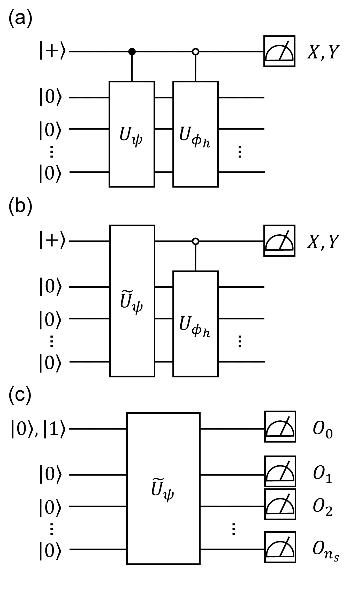
Figure 7: Quantum circuits for calculating the overlap. The topmost line represents the ancilla qubit and the other lines represent the system qubits. (a) The Hadamard test. (b) The pseudo-Hadamard test. (c) The VQE circuit with constraint to determine $\tilde{U}_{\psi}$ used for the pseudo-Hadamard test. The ancilla qubit is set to $\ket{0}$ when calculating the constraints.

We develop a gate-efficient technique to calculate the overlap executable on an arbitrary ansatz, called the pseudo-Hadamard test. See Appendix H for the extension of the technique to HTN. Figure 7(b) shows the circuit of the pseudo-Hadamard test, in which $U_{\psi}$ is replaced with $\tilde{U}_{\psi}$ involving the ancilla qubit. This circuit does calculate the overlap $\innerproduct{\tilde{\psi}}{\phi_{h}}$ if $\tilde{U}_{\psi}$ satisfies the following conditions:

$$\tilde{U}_{\psi}\ket{1}\ket{0}^{\otimes n_{s}}=\ket{1}\ket*{\tilde{\psi}},$$ (11)

$$\tilde{U}_{\psi}\ket{0}\ket{0}^{\otimes n_{s}}=\ket{0}\ket{0}^{\otimes n_{s}}.$$

In fact, the gate $\tilde{U}_{\psi}$ can be determined through the VQE, which is formulated as

$$\underset{\tilde{U}_{\psi}}{\min} \bra{1}\bra{0}^{\otimes n_{s}}\tilde{U}_{\psi}^{{\dagger}}(I\otimes H)\tilde{U}_{\psi}\ket{1}\ket{0}^{\otimes n_{s}}$$ (12)

s.t. $$\bra{1}\bra{0}^{\otimes n_{s}}\tilde{U}_{\psi}^{{\dagger}}(n_{0}\otimes I^{\otimes n_{s}})\tilde{U}_{\psi}\ket{1}\ket{0}^{\otimes n_{s}}=1,$$

$$\bra{0}\bra{0}^{\otimes n_{s}}\tilde{U}_{\psi}^{{\dagger}}(\sum_{j_{q}=0}^{n_{s}}I^{\otimes j_{q}}\otimes n_{j_{q}}$$

$$\quad\otimes I^{\otimes n_{s}-j_{q}})\tilde{U}_{\psi}\ket{0}\ket{0}^{\otimes n_{s}}=0,$$

where the index of the ancilla qubit is set to 0. Figure 7(c) shows the quantum circuit used to run such VQE, where $O_{i_{q}}$ ($i_{q}=0,1,\dots,n_{s}$) is an observable of the $i_{q}$-th qubit. The constraints can be relaxed through the appropriate selection of ansatz, such as the real amplitude ansatz without rotation gates on the ancilla qubit, as shown in Fig. 4(b). In this case, the VQE can be simplified as

$$\underset{\tilde{U}_{\psi}}{\min} \bra{1}\bra{0}^{\otimes n_{s}}\tilde{U}_{\psi}^{{\dagger}}(I\otimes H)\tilde{U}_{\psi}\ket{1}\ket{0}^{\otimes n_{s}}$$ (13)

s.t. $$\bra{0}\bra{0}^{\otimes n_{s}}\tilde{U}_{\psi}^{{\dagger}}(\sum_{j_{q}=1}^{n_{s}}I^{\otimes j_{q}}\otimes n_{j_{q}}$$

$$\quad\otimes I^{\otimes n_{s}-j_{q}})\tilde{U}_{\psi}\ket{0}\ket{0}^{\otimes n_{s}}=0.$$

We adopt this simplified formalism hereafter. Note that $\tilde{U}_{\psi}\ket{0}\ket{0}^{\otimes n_{s}}$ takes either $\ket{0}\ket{0}^{\otimes n_{s}}$ or $-\ket{0}\ket{0}^{\otimes n_{s}}$ in the constraint, but the signs cancel out in a numerator and denominator of $E_{mix}$ in both QC-QMC and HTN+QMC, allowing one to ignore the sign. In general, the sign might be able to be determined based on the overlap between a trial wave function and a specific standard basis state, e.g., the Hartree-Fock state [Xu2023-sn]. We also mention the extensions of the technique; a transition amplitude of $\matrixelement{\tilde{\psi}}{O}{\phi_{h}}$ can be calculated by the measurements of each system qubit in the basis corresponding to $O_{i_{q}}$ for the pseudo-Hadamard test circuit; that of $\matrixelement{\tilde{\psi}}{O}{\tilde{\psi}^{{}^{\prime}}}$ can be also calculated by the additional constraint as $\bra{1}\bra{0}^{\otimes n_{s}}\tilde{U}_{\psi}^{\dagger}\tilde{U}_{\psi^{{}^{\prime}}}^{\dagger}\tilde{U}_{\psi}(\sum_{j_{q}=1}^{n_{s}}I^{\otimes j_{q}}\otimes n_{j_{q}}\otimes I^{\otimes n_{s}-j_{q}})\tilde{U}_{\psi}^{\dagger}\tilde{U}_{\psi^{{}^{\prime}}}\tilde{U}_{\psi}\ket{1}\ket{0}^{\otimes n_{s}}=0$, where $\ket{\tilde{\psi}^{{}^{\prime}}}$ is a trial wave function defined by $\tilde{U}_{\psi^{{}^{\prime}}}$ with a property of $\tilde{U}_{\psi^{{}^{\prime}}}\ket{0}\ket{0}^{\otimes n_{s}}=\ket{0}\ket*{\tilde{\psi}^{{}^{\prime}}}$; a transition probability $\absolutevalue{\matrixelement{\tilde{\psi}}{O}{\tilde{\psi}^{{}^{\prime}}}}^{2}$ [Ibe2022-jp, Sawaya2023-wx] can be trivially obtained by the square of the transition amplitude.

We applied the pseudo-Hadamard test technique to the HTN+QMC calculations on a real device $ibmq\_kolkata$ for the hydrogen plane model with ID 3 and MABI. The best trial wave function was selected from 100 seeds of HTN+VQE runs under the constraint ($\tilde{d}_{H}=4$ and statevector execution), where at most five qubits including an ancilla qubit are used in the overlap calculation. See Appendix H.1 for details on the extension to HTN. Figure 8(a) shows the result for the hydrogen plane model. A smaller fluctuation around the exact ground state energy was found in HTN+QMC than in QMC. The standard deviations obtained by the QMC, HTN+QMC (statevector) and HTN+QMC ($ibmq\_kolkata$) methods are $6.7\times 10^{-3},1.5\times 10^{-3}$, and $2.0\times 10^{-3}$ Hartree, respectively. Importantly, there is only a slight difference in the fluctuation between the real device and statevector, indicating that there would be some robustness of HTN+QMC to noises. The previous study [Huggins2022-ly] showed that QC-QMC is robust to the depolarization noise, and we found by the analysis shown in Appendix H.2 that such robustness also holds in the current settings of HTN+QMC. The MABI results in Fig. 8(b) also showed high accuracy in the real device experiment, where the standard deviations are $2.6\times 10^{-3},1.6\times 10^{-3}$, and $1.8\times 10^{-3}$ Hartree in the above three methods, respectively. These numerical and theoretical results suggest that HTN+QMC can be a promising candidate for calculating large systems beyond the scale of quantum devices while maintaining accuracy. Note that although we utilized the readout error mitigation and the dynamic decoupling in the overlap calculation, we confirmed that a comparable level of accuracy was achieved even without those options in HTN+QMC for the hydrogen plane model, where the standard deviation without the options is $1.5\times 10^{-3}$ Hartee.

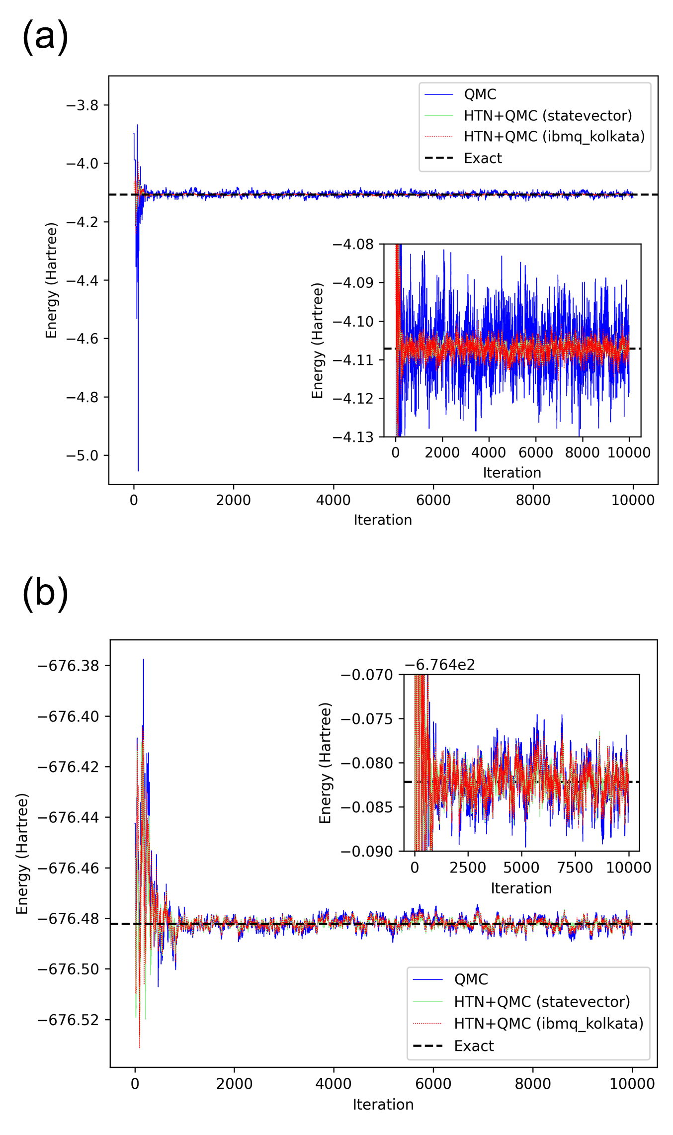
Figure 8: Results of the energy on the real device execution for the hydrogen plane model and MABI. HOMO-LUMO setting and $\tilde{d}_{H}=4$ are adopted for the models. The blue line represents the QMC result, the light green and red lines respectively represent the HTN+QMC results of statevector and real device procedures, and the black dashed line represents the exact ground state energy. (a) The result of the hydrogen plane model with $n=4$ and $k=2$. (b) The result of MABI with $n=4$ and $k=3$. The inset in each figure is an enlarged view along the y-axis.

III Discussion

We proposed an algorithm HTN+QMC that combines QC-QMC with HTN for accurately calculating problems in quantum chemistry beyond the size of a quantum device: (1) QC-QMC can perform electronic structure calculation with higher accuracy than either VQE or QMC alone by using a trial wave function prepared on quantum devices, (2) HTN enables us to construct a large wave function beyond the size of a quantum device by decomposing the wave function into smaller-size tensors, which are computed by hybrid quantum/classical methods. Specifically, the two-layered QQTN, which is one of the HTN structures, allows QC-QMC to prepare $\order{n^{2}}$-qubit trial wave function by using only $\order{n}$ qubit devices.

The trial wave function prepared by HTN+VQE is used to execute HTN+QMC, where FCIQMC is adopted as a QMC method. As demonstrated on the benchmarking models, we found that HTN+QMC exhibits energy accuracy that is several orders of magnitude higher than HTN+VQE or QMC. In addition, HTN+QMC will outperform QC-QMC (i.e., without HTN), if the interaction between the decomposed subsystems becomes small, that is, if the target state is close to a separable or low entangled product state in a suitably chosen decomposition setting. We developed the gate-efficient pseudo-Hadamard test technique involving an ancilla qubit, for the purpose of conducting the HTN+QMC experiments on real devices; the at most five qubits experiment showed an accuracy comparable to the statevector simulation for the hydrogen plane models (8 qubit model) and MABI (12 qubit model).

While this study assumed that the size of the target system is larger than that of the quantum device, there may be cases in which the proposed algorithm should be used even if the size of the target system is the same as that of the quantum device. For example, a quantum computer with thousands of qubits will appear in the near future [Matthews2021-pl], but due to noise in the quantum device, it is possible that an accurate solution may not be obtained in the calculation of a chemical model of that size. In such a case, decomposing the system into subsystems of about hundreds of qubits would lead to a more accurate result than that obtained by directly executing on a thousand qubits.

The research on QC-QMC has not yet been extensive, and the application of techniques developed for NISQ devices to QC-QMC is a possible future research item, as in HTN in this study. Another interesting direction is the application of QC-QMC to the fields outside the electronic structure calculations such as machine learning for designing advanced materials.

IV Methods

IV.1 Variational quantum eigensolver

VQE takes a variational approach to obtain the ground state of a given Hamiltonian, where a trial wave function $\ket{\psi(\vec{\theta})}$ is generated by a quantum circuit with variational parameters $\vec{\theta}$, which is repeatedly updated using the classical computer until a termination condition is satisfied, e.g., the expectation value of the Hamiltonian $\bra{\psi(\vec{\theta})}H\ket{\psi(\vec{\theta})}$ takes a minimum. The expressibility of $\ket{\psi(\vec{\theta})}$ depends on the quantum circuit, what is called ansatz. There are several problem-inspired ansatze such as the unitary coupled cluster ansatz [Taube2006-jj] and Hamiltonian variational ansatz [Wecker2015-fu], and despite the high performance, the ansatze require deeper quantum gates. In real device experiments, compromised strategy with hardware-efficient ansatze  [Kandala2017-lh] is often taken.

The Hamiltonian $H$ in the electronic structure problems can be represented as

$$H=\sum_{a}c_{a}\bigotimes_{b}P_{ab},$$ (14)

where $c_{a}$ is the $a$-th coefficient of $H$, $P_{ab}\in\{X,Y,Z,I\}$ is the $a$-th Pauli or identity operator on the $b$-th site. In this study, $c_{a}\in\mathbb{R}$ is assumed for all the models ($c_{a}\in\mathbb{C}$ in general). The number of terms is estimated to be $\order{N_{so}^{4}}$ with $N_{so}$ being the number of spin-orbitals [Tilly2022-pb]. We choose the Jordan-Wigner mapping [Jordan1928-hf] for the fermion-qubit translation.

IV.2 Quantum computing quantum Monte Carlo

In QC-QMC Ref. [Huggins2022-ly], a stochastic algorithm such as the imaginary-time evolution is used to iteratively update the discretized coefficients of the wave function i.e., walkers. There are two approaches to integrate the quantum computations: one is to use it only for the energy evaluation [Xu2023-sn], and the other for the energy evaluation and walker control [Huggins2022-ly, Zhang2022-lf, Xu2023-sn]. The latter approach, which is more effective in mitigating the sign problem, is computationally expensive [Xu2023-sn]. We adopt the former approach which is easier to execute on a real device. The following mixed energy $E_{mix}$ is used as a common energy estimator:

$$E_{mix} =\frac{\bra{\xi}H\ket{\psi_{QMC}}}{\innerproduct{\xi}{\psi_{QMC}}},$$ (15)

where $\ket{\xi}$ is a trial wave function. $\ket{\psi_{QMC}}$ denotes a wave function generated by QMC, which is defined by

$$\ket{\psi_{QMC}} =\sum_{h}w_{h}\ket{\phi_{h}},$$ (16)

where $w_{h}$ is the ${h}$-th coefficient and is expressed using discretized units (walkers). $\ket{\phi_{h}}$ is the ${h}$-th standard basis state as in a Slater determinant and can be represented by a binary string i.e., a computational basis. The procedure of generating the wave function $\ket{\psi_{QMC}}$ depends on the method of QMC. In this work, we chose FCIQMC. See Appendix A for the details of its procedure. $E_{mix}$ is not exactly equivalent to the expectation value of the Hamiltonian $\matrixelement{\psi_{QMC}}{H}{\psi_{QMC}}/\innerproduct{\psi_{QMC}}{\psi_{QMC}}$ (that is, not the pure estimator), but we can obtain the exact ground state energy $E_{g}$ when $\ket{\psi_{QMC}}$ approaches to the ground state $\ket{\psi_{g}}$, i.e., $\ket{\psi_{QMC}}\sim\ket{\psi_{g}}$ as

$$E_{mix} \sim\frac{\bra{\xi}H\ket{\psi_{g}}}{\innerproduct{\xi}{\psi_{g}}}=E_{g},$$ (17)

where $H\ket{\psi_{g}}=E_{g}\ket{\psi_{g}}$ is used. When the sign problem occurs, the statistical error for evaluating $E_{mix}$ becomes exponentially large [Troyer2005-bk]. For example in FCIQMC, for basis states with small $w_{h}$, the sign of $w_{h}$ fluctuates over the iterations by competing positive and negative walker counts [Spencer2012-wq, Kolodrubetz2013-ke]. However, by using a trial wave function $\ket{\xi}$ that incorporates the electron correlations correctly, we can mitigate the sign problem. A trivial case is that, if the trial wave function coincides with the ground state, i.e., $\ket{\xi}=\ket{\psi_{g}}$, then we can obtain $E_{g}$ for any $\ket{\psi_{QMC}}$ with zero variance [Apaja2018-fi]. See Appendix B for a detail of the derivation. In contrast, the trial wave functions that are conveniently available in classical computations, such as the Hartree-Fock state, the linear combination of mean-field states, and the Jastrow-type states [Austin2012-qi] may easily bring about the sign problem. Therefore, if we can only prepare a suboptimal trial wave function in the exponentially large Hilbert space, we can considerably minimize the errors in the energy estimation.

In QC-QMC, the trial wave function $\ket{\xi}$ is prepared by a quantum algorithm. Specifically, by decomposing $\ket{\psi_{QMC}}$, Eq. (15) is rewritten as

$$E_{mix} =\frac{\sum_{h^{\prime}{h}}w_{h^{\prime}}\innerproduct{\xi}{\phi_{h}}\bra{\phi_{h}}H\ket{\phi_{h^{\prime}}}}{\sum_{{h}}w_{h}\innerproduct{\xi}{\phi_{h}}}.$$ (18)

The matrix elements $\bra{\phi_{h}}H\ket{\phi_{h^{\prime}}}$ can be obtained by trivial classical calculations. In contrast, quantum computation is required to calculate the overlap $\innerproduct{\xi}{\phi_{h}}$, for which we can apply the Hadamard test or the classical shadow [Huang2020-ld, Zhao2021-kw]. We discuss in Appendix B that the variance of the mixed energy will decrease with the fidelity of the trial wave function in a simplified case. In this study, fidelity is defined as the square of the overlap between the target and ground states assuming the absence of noises.

IV.3 Hybrid tensor network

In the two-layer QQTN, the original $nk$-qubit system is decomposed into $k$ subsystems of $n$ qubit states $\ket{\varphi^{i_{m}}}$, which are combined together and integrated with the $k$-qubit state $\ket{\psi}$. These states can be associated with tensors, which are defined as $\varphi_{\vec{j}_{m}}^{i_{m}}=\innerproduct{\vec{j}_{m}}{\varphi^{i_{m}}}$ and $\psi_{\vec{i}}=\innerproduct{\vec{i}}{\psi}$ with the vector indices $\vec{j}_{m}=j_{m1}j_{m2}\dots j_{mn}$ and $\vec{i}=i_{1}i_{2}\dots i_{k}$ in $n$-qubit and $k$-qubit binary strings, respectively. We call the former a lower tensor and the latter an upper tensor, respectively. The wave function $\ket{\psi_{HTN}}$ is then decomposed into tensor products of $\ket{\varphi^{i_{m}}}$

$$\ket{\psi_{HTN}} =\sum_{\vec{i}}\psi_{\vec{i}}\bigotimes_{m=1}^{k}\ket{\varphi^{i_{m}}},$$ (19)

which is the same as Eq. (1) although omitting the parameters, where the number of vector coefficients $\{\psi_{\vec{i}}\}$ is $2^{Lk}$ with $L$ denoting the number of bits (legs) used to construct each $i_{m}$. $L=1$ is adopted in this study. If $L=n$, $\ket{\psi_{HTN}}$ becomes the general $nk$-qubits wave function. When $L\ll n$, $\ket{\psi_{HTN}}$ lives in a subspace much smaller than the entire $2^{nk}$ dimensional Hilbert space, although it can be larger than the subspace consisting only of the classical tensor due to the exponentially large ranks of $\psi_{\vec{i}}$ and $\varphi^{i_{m}}_{\vec{j}_{m}}$, and the performance of the QQTN depends on the decomposition setting of the system, which determines the entanglement between the subsystems.

There is a variety of tensor implementations in a quantum circuit. For example, we can define a lower tensor as $\ket{\varphi^{i_{m}}}=U_{Lm}\ket{i_{m}}\ket{0}^{\otimes n-1}$, $U_{Lm}\ket{i_{m}}^{\otimes n}$, $U_{Lm}^{i_{m}}\ket{0}^{\otimes n}$, etc., where the first two formulations give the index in initial states and the third a unitary matrix by using unitary matrices $U_{Lm}$ and $U_{Lm}^{i_{m}}$. In the present study, we choose $\ket{\varphi^{i_{m}}}=U_{Lm}\ket{i_{m}}\ket{0}^{\otimes n-1}$ and $\ket{\psi}=U_{U}\ket{0}^{\otimes k}$ for lower and upper tensors, respectively.

In our QQTN formulation, an observable is defined as a tensor product $O=\bigotimes_{m,r}O_{mr}$, where $O_{mr}$ is observable on the $r$-th qubit of the $m$-th subsystem (lower tensor). Transition amplitude is then defined as

$$T=\matrixelement{\psi_{HTN}^{(1)}}{O}{\psi_{HTN}^{(2)}},$$ (20)

which is the same as Eq. (2) although omitting the parameters, where $\ket{\psi_{HTN}^{(l)}}=\sum_{\vec{i}}\psi_{\vec{i}}^{(l)}\bigotimes_{m}\ket{\varphi^{i_{m}(l)}}(l=1,2)$ are the two different of states for $\ket{\psi_{HTN}}$. As will be explained in the next section, $T$ is used both in VQE and QMC to evaluate an observable and overlap, respectively.

We first calculate $N^{i_{m}^{\prime}(1)i_{m}(2)}=\matrixelement{\varphi^{i_{m}^{\prime}(1)}}{\bigotimes_{r}O_{mr}}{\varphi^{i_{m}(2)}}$ for the lower tensors by quantum computations, construct $N_{m}=\matrixquantity(N^{00}&N^{01}\\ N^{10}&N^{11})$, which is a trivial classical process, and then integrate the results as $T=\matrixelement{\psi^{(1)}}{\bigotimes_{m}N_{m}}{\psi^{(2)}}$ on the upper tensor by quantum computations. Appendix C shows the details of this procedure, which is based on the circuit of the Hadamard test as in Ref. [Kanno2021-zn]. Our algorithm requires only $\max(n,k)$ qubits except for ancilla qubits. In this study, only $8k+2$ terms are measured in the $T$ calculation, i.e., the overhead for calculating the expectation value is a linear scale in the system size $nk$. Note that the number of measurements is $2\times 4^{L}k+2$ in general.

IV.4 Proposed algorithm: HTN+QMC

The procedure of HTN+QMC consists of two steps.

1. Perform VQE by minimizing $\bra{\psi_{HTN}}H\ket{\psi_{HTN}}$ to obtain the trial wave function $\ket{\xi}=\ket{\psi_{HTN}}$.

2. Perform QC-QMC by using the obtained trial wave function $\ket{\psi_{HTN}}$; the quantum computer is used to compute $E_{mix}$ to accurately estimate the ground state energy.

Here, we will denote HTN+VQE when only the first step is mentioned. HTN+QMC can be performed for $nk$-qubit system by using only $\order{\mathrm{max}(n,k)}$ qubits except for ancilla qubits. Specifically, if $k\sim n$, an $\order{n^{2}}$-qubit trial wave function is prepared only by an $\order{n}$-qubit circuit. In both steps, the Hamiltonian and mixed energy can be evaluated through the calculations of $T$ in Eq. (20).

In the first step, by splitting the index $b$ in Eq. (14) into the two indices $m$ and $r$, we can rewrite $H$ and its expectation value as

$$H =\sum_{a}c_{a}\bigotimes_{m,r}P_{amr},$$ (21)

and

$$\bra{\psi_{HTN}}H\ket{\psi_{HTN}} =\sum_{a}c_{a}\bra{\psi_{HTN}}\bigotimes_{m,r}P_{amr}\ket{\psi_{HTN}},$$ (22)

respectively. The expectation value is evaluated through Eq. (20) by setting $\ket{\psi_{HTN}^{(1)}}=\ket{\psi_{HTN}^{(2)}}=\ket{\psi_{HTN}}$ and replacing $O_{mr}$ with $P_{amr}$, where the coefficient index $a$ is regarded as implicitly included in the expression of $O_{mr}$. The wave function $\ket{\psi_{HTN}}$ is prepared by parameterized quantum circuits equivalent to the unitary matrices $U_{Lm}$ and $U_{U}$.

In the second step, the overlap $\innerproduct{\xi}{\phi_{h}}=\innerproduct{\psi_{HTN}}{{\phi_{h}}}$ in Eq. (18) is calculated by substituting $\ket{\psi_{HTN}^{(1)}}=\ket{\psi_{HTN}}$, $\ket{\psi_{HTN}^{(2)}}=\ket{\phi_{h}}$, and $O=I^{\otimes nk}$ in $T$ of Eq. (20), where the circuit parameters are fixed to the values obtained in the first step. More specifically, we can prepare an arbitrary basis state $\ket{\phi_{h}}=\bigotimes_{m,r}\ket{j_{mr}(h)}=(\bigotimes_{m,r}X^{j_{mr}(h)})\ket{0}^{\otimes nk}$ by setting $U_{U}^{(2)}=I^{\otimes k}$ and $U_{Lm}^{(2)}=\bigotimes_{m}X^{j_{mr}(h)}$, where $j_{mr}(h)$ is a function of $h$, $j_{mr}(h)$ takes a value on $\{0,1\}$, and $X$ is a Pauli $X$ operator. Having the overlaps $\innerproduct{\psi_{HTN}}{\phi_{h}}$ of all $\ket{\phi_{h}}$ corresponding to the walkers appearing during the QMC execution at hand, we can perform QMC through iterative evaluations of the mixed energy (Eqs. (15) and (16)).

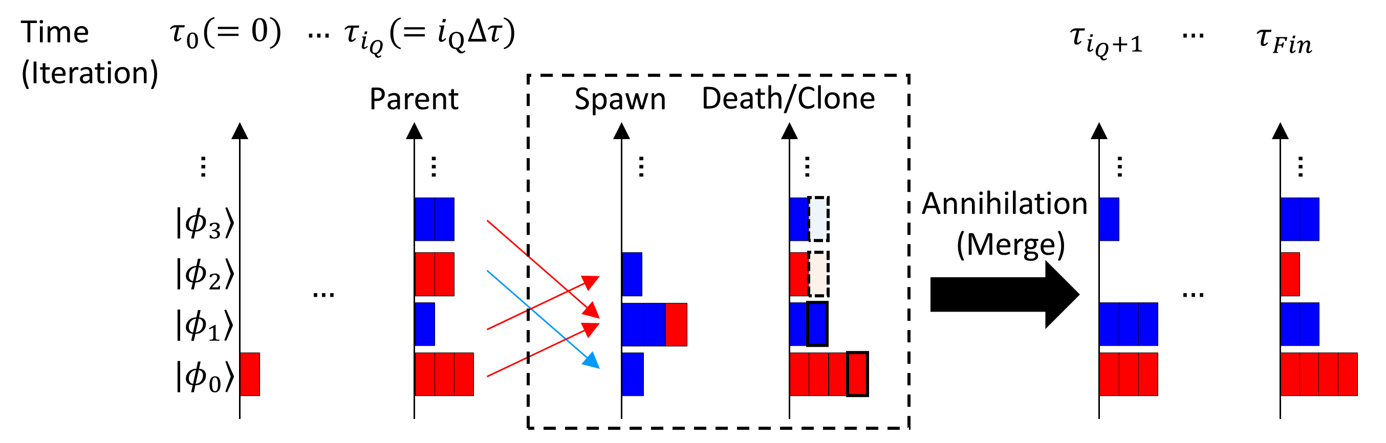
Figure 9: Procedure of FCIQMC. The walker of $\ket{\phi_{h}}$ with a plus (minus) sign is represented as a red (blue) rectangle.

Appendix A Procedure of full configuration interaction quantum Monte Carlo

In FCIQMC, the wave function $\ket{\psi_{QMC}}$ is defined as

$$\ket{\psi_{QMC}} =\sum_{h}w_{h}\ket{\phi_{h}},$$ (23)

where $w_{h}$ is the real coefficient of $h$-th standard basis state (such as the Slater determinant) $\ket{\phi_{h}}$. Those coefficients will be updated iteratively through the imaginary time evolution according to

$$\frac{dw_{h^{\prime}}}{d\tau} =-\sum_{h}(H_{h^{\prime}h}-S\delta_{h^{\prime}h})w_{h},$$ (24)

which can be written in a discrete form as

$$\Delta w_{h^{\prime}} =-\sum_{h\neq h^{\prime}}H_{h^{\prime}h}\Delta\tau\times w_{h}-(H_{hh}-S)\Delta\tau\times w_{h},$$ (25)

where $H_{h^{\prime}{h}}=\bra{\phi_{h^{\prime}}}H\ket{\phi_{h}}$ is a matrix element of the Hamiltonian, $\delta_{h^{\prime}h}$ is the Kronecker delta, $\tau$ is an imaginary time, $\Delta\tau$ is a time increment, and $S$ is an energy shift. The first and second terms are contributions from the off-diagonal and diagonal elements of the Hamiltonian, respectively.

The procedure of FCIQMC is illustrated in Fig. 9. The walker with the positive (negative) sign is depicted as red (blue) rectangular. The imaginary time in the $i_{Q}$-th iteration is denoted by $\tau_{i_{Q}}$. For the walkers in the $i_{Q}$-th iteration, called the parent walkers, the following operations are performed to obtain the $i_{Q}+1$-th walkers.

• Spawning step [the off-diagonal terms in Eq. (25)]: For each parent walker with index ${h}$, a new walker with index ${h^{\prime}}$ is generated with a probability of $\absolutevalue{H_{h^{\prime}{h}}}\Delta\tau$, to which $\operatorname{sgn}(-H_{h^{\prime}{h}})$ is assigned. If $\absolutevalue{H_{h^{\prime}{h}}}\Delta\tau>1$, however, $\lfloor\absolutevalue{H_{h^{\prime}{h}}}\Delta\tau\rfloor$ walkers and a walker are generated with a probability of 1 and $\absolutevalue{H_{h^{\prime}{h}}}\Delta\tau-\lfloor\absolutevalue{H_{h^{\prime}{h}}}\Delta\tau\rfloor$, respectively.

• Death/cloning step [the diagonal term in Eq. (25)]: For each parent walker with an index ${h}$, remove (copy) walkers of the same index with probability $\absolutevalue{(H_{h^{\prime}{h}}-S)}\Delta\tau$ if the sign of $(H_{h^{\prime}{h}}-S)\Delta\tau$ is positive (negative). If $\absolutevalue{(H_{h^{\prime}{h}}-S)}\Delta\tau>1$, remove (copy) the walkers with probability 1.

• Annihilation step: Merge the walkers obtained in the spawning and death/cloning steps. The walkers with opposite signs are canceled out.

In the death/cloning step, the initial value of $S$ is a constant (e.g., the value of the Hartree-Fock energy), and when the number of walkers exceeds the set value $N_{shift}$, $S$ is updated every $A$ iteration as $S(\tau_{i_{Q}})=S(\tau_{i_{Q}}-A\Delta\tau)-\frac{\zeta}{A\Delta\tau}\ln\frac{N_{W}(\tau_{i_{Q}})}{N_{W}(\tau_{i_{Q}}-A\Delta\tau)}$ so that the number of the walkers remains constant (called variable shift mode), where $S(\tau_{i_{Q}})$ is $S$ on the time $\tau_{i_{Q}}$, $\zeta$ is a damping parameter, and $N_{W}(\tau_{i_{Q}})$ is the number of walkers on $\tau_{i_{Q}}$. We note that although the computational cost, i.e., the number of walkers required by this algorithm, may increase exponentially with the size of the system in general, there are several proposals to make the algorithms executable for practical systems  [Booth2009-lv, Cleland2010-au, Petruzielo2012-rk, Guther2020-um]. For example, the number of walkers required for $\mathrm{N_{2}}$ molecule can be reduced by three orders of magnitude ($10^{8}$ to $10^{5}$) by restricting spawning only on the basis state for which the number of walkers exceeds a certain threshold [Cleland2010-au].

Finally, the other calculation conditions that are not described in Sec. II.1 are the following. The initial value of the energy shift $S$ was set to the energy of the leading single reference state in the standard basis state of the ground state (the ground state when constrained to six electrons in MABI). The imaginary time increment $\Delta\tau$ was 0.001 $\mathrm{Hartree}^{-1}$ for the Heisenberg chain and graphite models, and 0.1 $\mathrm{Hartree}^{-1}$ for the hydrogen plane model and MABI. The parameters for the variable shift were $N_{shift}=1000$, $A=5$, and $\zeta=0.1$.

Appendix B Statistical analysis of mixed energy in simple cases

Here, in the simple cases, we discuss the statistical error of the mixed energy, which arises from preparing the trial wave function by a quantum algorithm. Let $\epsilon$ and $(1-F)$ denote the deviations of the wave function generated by QMC $\ket{\psi_{QMC}}$ and the trial wave function $\ket{\xi}$ from the ground state $\ket{\psi_{g}}$, the wave functions can be represented as

$$\ket{\psi_{QMC}(\epsilon)} =(1-\epsilon)\ket{\psi_{g}}+\epsilon\sum_{s}u_{s}\ket{\psi_{s}^{\perp}},$$ (26)

and

$$\ket{\xi(F)} =F\ket{\psi_{g}}+(1-F)\sum_{s^{\prime}}v_{s^{\prime}}\ket{\psi_{s^{\prime}}^{\perp}},$$ (27)

respectively. $F^{2}$ is a fidelity of $\ket{\xi(F)}$, $\ket{\psi_{s}^{\perp}}$ and $\ket{\psi_{s^{\prime}}^{\perp}}$ are the orthogonal states with the coefficients $\ket{\psi_{g}}$, $u_{s}$ and $v_{s^{\prime}}$, and $\epsilon,F\in[0,1]$. The mixed energy $E_{mix}(\epsilon;F)$ can be then described as

$$E_{mix}(\epsilon;F) =\frac{\bra{\xi(F)}H\ket{\psi_{QMC}(\epsilon)}}{\innerproduct{\xi(F)}{\psi_{QMC}(\epsilon)}}$$ (28)

$$=\frac{(1-\epsilon)FE_{g}+\epsilon(1-F)\sum_{s}E_{s}u_{s}v_{s}}{(1-\epsilon)F+\epsilon(1-F)\sum_{s}u_{s}v_{s}},$$

with the ground state energy $E_{g}$ and eigenvalue of $\ket{\psi_{s}^{\perp}}$ denoted by $E_{s}$. Below, we assume $E_{g}=0$ without loss of generality. Then the mean and variance of $E_{mix}(\epsilon;F)$, $\mathbb{E}(E_{mix}(\epsilon;F))$ and $Var(E_{mix}(\epsilon;F))$, are respectively represented as

$$\mathbb{E}(E_{mix}(\epsilon;F)) =\mathbb{E}\left(\frac{\epsilon(1-F)\sum_{s}E_{s}u_{s}v_{s}}{(1-\epsilon)F+\epsilon(1-F)\sum_{s}u_{s}v_{s}}\right),$$ (29)

and

$$Var(E_{mix}(\epsilon;F)) =\mathbb{E}(E_{mix}(\epsilon;F)^{2})-\mathbb{E}(E_{mix}(\epsilon;F))^{2}$$ (30)

$$=\mathbb{E}\left(\frac{\{\epsilon(1-F)\sum_{s}E_{s}u_{s}v_{s}\}^{2}}{\{(1-\epsilon)F+\epsilon(1-F)\sum_{s}u_{s}v_{s}\}^{2}}\right)$$

$$-\mathbb{E}\left(\frac{\epsilon(1-F)\sum_{s}E_{s}u_{s}v_{s}}{(1-\epsilon)F+\epsilon(1-F)\sum_{s}u_{s}v_{s}}\right)^{2},$$

where the integral variable of the expected value is the QMC time step, on which $\epsilon$ and $u_{s}$ depend. Now consider $\mathbb{E}(E_{mix}(\epsilon;F))$ and $Var(E_{mix}(\epsilon;F))$ in the two cases. In the first case of $F=1$, both $\mathbb{E}(E_{mix}(\epsilon;F))$ and $Var(E_{mix}(\epsilon;F))$ are trivially zero, that is, if the trial wave function is the ground state, $E_{mix}$ is equal to the ground state energy regardless of $\ket{\psi_{QMC}(\epsilon)}$ (excluding $\epsilon=1$).

In the second case, where $E_{mix}(\epsilon;F)$ fluctuates around the ground state energy in a small amount, assuming $\mathbb{E}(E_{mix}(\epsilon;F))=0$ and the expected value of the higher order terms of $\epsilon$ be negligible, the variance becomes

$$Var(E_{mix}(\epsilon;F)) =\mathbb{E}\left(\frac{\{\epsilon(1-F)\sum_{s}E_{s}u_{s}v_{s}\}^{2}}{\{(1-\epsilon)F+\epsilon(1-F)\sum_{s}u_{s}v_{s}\}^{2}}\right)$$ (31)

$$=\mathbb{E}\left(\frac{(1-F)^{2}}{F^{2}}(\sum_{s}E_{s}u_{s}v_{s})^{2}\epsilon^{2}+\order{\epsilon^{3}}\right)$$

$$=\order{\left(\frac{1-F}{F}\right)^{2}}.$$

$\left(\frac{1-F}{F}\right)^{2}$ is monotonically decreasing, and thus when the fidelity of the trial wave function in the quantum algorithm is larger than that in the classical algorithm, we can expect a decrease in the variance of the mixed energy.

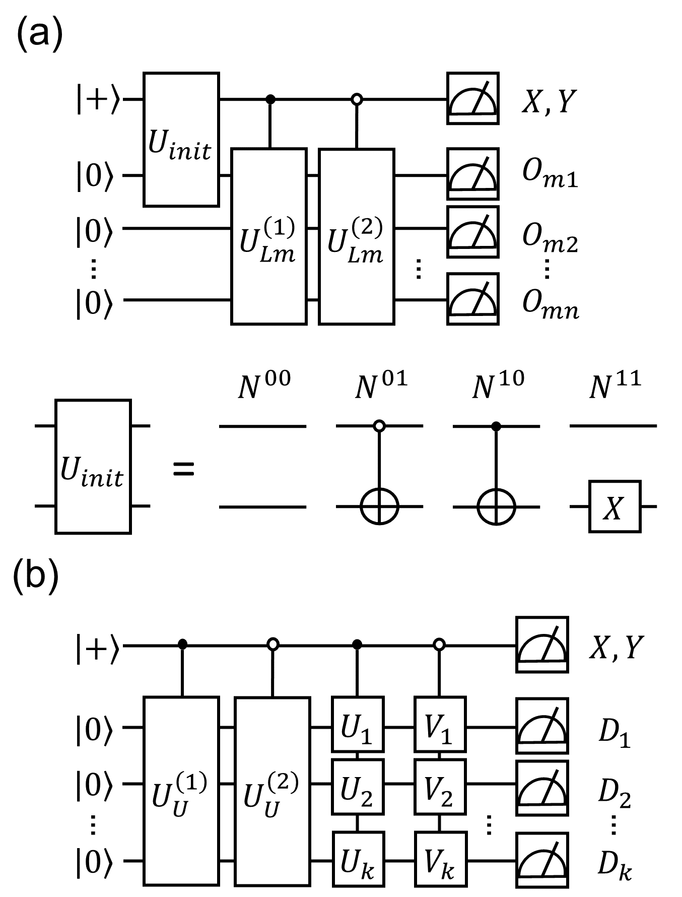
Figure 10: Quantum circuits for calculating $T$. The topmost line represents an ancilla qubit and the other lines represent system qubits. (a) The calculation for the lower tensor. (b) The calculation for the upper tensor.

Appendix C Calculation of the transition amplitude by using HTN

We explain the procedure for calculating $T$ in Eq. (20) based on the Hadamard test [Kanno2021-zn], which is reproduced as

$$T =\sum_{\vec{i}^{\prime}~{}\vec{i}}\psi_{\vec{i}^{\prime}}^{(1)*}\psi_{\vec{i}}^{(2)}\prod_{m=1}^{k}\matrixelement{\varphi^{i_{m}^{\prime}(1)}}{\bigotimes_{r}O_{mr}}{\varphi^{i_{m}(2)}}$$ (32)

$$=\sum_{\vec{i}^{\prime}~{}\vec{i}}\psi_{\vec{i}^{\prime}}^{(1)*}\psi_{\vec{i}}^{(2)}\prod_{m=1}^{k}N^{i_{m}^{\prime}i_{m}}.$$

The first part includes the calculations of the matrices $N^{i_{m}^{\prime}i_{m}}$ for the lower tensors. Figure 10(a) shows the quantum circuit for this purpose when the state in the lower tensor is defined by $\ket{\varphi^{i_{m}(l)}}=U_{Lm}^{(l)}\ket{i_{m}(l)}\ket{0}^{\otimes n-1}$. $U_{init}$ is one of the circuits in the lower panel, which is selected for each of the matrix elements $N^{00},N^{01},N^{10}$, or $N^{11}$, and creates the superposed state $\frac{1}{\sqrt{2}}(\ket{1}\ket{i_{m}^{\prime}(1)}\ket{0}^{\otimes n-1}+\ket{0}\ket{i_{m}(2)}\ket{0}^{\otimes n-1})$, which is then transformed to $\frac{1}{\sqrt{2}}(\ket{1}U_{Lm}^{(1)}\ket{i_{m}^{\prime}(1)}\ket{0}^{\otimes n-1}+\ket{0}U_{Lm}^{(2)}\ket{i_{m}(2)}\ket{0}^{\otimes n-1})$ through $U_{Lm}^{(1)}$ and $U_{Lm}^{(2)}$ operations, and measured in the measurement basis corresponding to $O_{mr}$. We can obtain the real and imaginary parts of $N^{i_{m}^{\prime}i_{m}}$ ($\real(N^{i_{m}^{\prime}i_{m}})$ and $\imaginary(N^{i_{m}^{\prime}i_{m}})$) by specifying respective $X$ and $Y$ for the measurement basis on the ancilla qubit. Calculation of $N^{i_{m}^{\prime}i_{m}}$ for each lower tensor, therefore, requires $4\times 2=8$ different measurements, where factor 4 comes from $N^{00},N^{01},N^{10}$, and $N^{11}$, and the factor 2 from $\real(N^{i_{m}^{\prime}i_{m}})$ and $\imaginary(N^{i_{m}^{\prime}i_{m}})$.

The second part is the calculation of the upper tensor. In terms of the upper tensor state, $T$ can be rewritten as

$$T =\sum_{\vec{i}^{\prime}~{}\vec{i}}\psi_{\vec{i}^{\prime}}^{(1)*}\psi_{\vec{i}}^{(2)}\prod_{m=1}^{k}N^{i_{m}^{\prime}i_{m}}$$ (33)

$$=\bra{\psi^{(1)}}\bigotimes_{m=1}^{k}N_{m}\ket{\psi^{(2)}},$$

where the $2\times 2$ non-Hermitian matrix $N_{m}$ is reformulated by the singular value decomposition (SVD),

$$T =\bra{\psi^{(1)}}\bigotimes_{m=1}^{k}U_{m}^{{\dagger}}D_{m}V_{m}\ket{\psi^{(2)}},$$ (34)

where $N_{m}=U_{m}^{{\dagger}}D_{m}V_{m}$, $U_{m}$ and $V_{m}$ are unitary matrices, and $D_{m}$ is a diagonal matrix. Since $N_{m}$ is a $2\times 2$ matrix, the SVD can be executed classically. The quantum circuit for calculating Eq. (34) is shown in Figure 10(b), where the superposed state $\frac{1}{\sqrt{2}}(\ket{1}U_{U}^{(1)}\ket{0}^{\otimes k}+\ket{0}U_{U}^{(2)}\ket{0}^{\otimes k})$ is transformed to $\frac{1}{\sqrt{2}}(\ket{1}\bigotimes_{m=1}^{k}U_{m}U_{U}^{(1)}\ket{0}^{\otimes k}+\ket{0}\bigotimes_{m=1}^{k}V_{m}U_{U}^{(2)}\ket{0}^{\otimes k})$ through $\bigotimes_{m=1}^{k}U_{m}$ and $\bigotimes_{m=1}^{k}V_{m}$, and measured in the computational basis. The measurement result, $\ket{0}$ or $\ket{1}$ gives the diagonal element of $D_{m}$, i.e., $(D_{m})_{00}$ or $(D_{m})_{11}$, respectively [Kanno2021-zn]. The real and imaginary parts of $T$ can be obtained by specifying $X$ and $Y$ for the measurement basis on the ancilla qubit, respectively. The calculation for the upper tensor thus requires measurements on two different bases. In total, the calculations of the lower and upper tensor require $8k+2$ sets of measurements, i.e., the overhead for calculating the expectation value is a linear scale for the system size $nk$. Note that when the Hamiltonian and wave function are real as in this study, the calculations of the real parts in the lower and upper tensors are unnecessary, reducing the overhead to $4k+1$. We additionally note that the QQTN can be expressed as a $nk$-qubit quantum circuit $(\prod_{m}U_{Lm}^{(l)})U_{U}^{(l)}(\bigotimes_{m}\ket{0}^{\otimes n})$ under the current assumption of $\ket{\varphi^{i_{m}(l)}}$ and $\ket{\psi^{(l)}}$, where $U_{Lm}^{(l)}$ operates qubits corresponding to $m$-th subsystem (i.e., $m$-th $\ket{0}^{\otimes n}$), and $U_{U}^{(l)}$ operates the qubits corresponding the first qubit of each subsystem [Yuan2021-ih]. As a final remark, the robustness of the barren plateau in this type of circuit has been reported [Martin2022-pj].

Appendix D Methods and conditions for constructing specific benchmarking models

For the graphite, we first calculated the band structure using density functional theory in the Quantum ESPRESSO package [Giannozzi2009-zq, Giannozzi2017-jz, Giannozzi2020-yi], in which we adopted the generalized gradient approximation by Perdew-Burke-Ernzerhof (PBE) [Perdew1996-qc] as the exchange-correlation functional and optimized norm-conserving Vanderbilt (ONCV) pseudopotential [Hamann1979-ti, Hamann2013-tx]. The wave function cutoff, k-point grids, and the number of bands were 64 Rydberg, $8\times 8\times 3$, and 30, respectively. Then we calculated $t_{1}$, $t_{2}$, and $U$ for target orbitals using the maximally localized Wannier function [Marzari1997-sz, Souza2001-un] and constrained random phase approximation [Aryasetiawan2004-sq] in the RESPACK package [Fujiwara2003-xg, Nakamura2008-hg, Nohara2009-rm, Nakamura2009-te, Nakamura2016-vj, Nakamura2021-sh]. The target orbitals were the four $p_{z}$ orbitals in each carbon atom in the unit cell. The polarization-function cutoff was 6.4 Rydberg. We obtained $t_{1}=-1.05\times 10^{-1}$, $t_{2}=1.03\times 10^{-2}$, and $U=3.00\times 10^{-1}$ Hartree.

The MABI structure was determined by $\mathrm{S_{0}}$ state geometry optimization at the three-state-averaged CASSCF(14e,14o)/6-31G level using Molpro 2015 [Werner2012-ky, Werner2020-ph], where MABI geometry in Cartesian coordinates is shown in Table 2. The PySCF package [Sun2020-hs] was adopted for constructing the Hamiltonian for the hydrogen plane models and MABI with STO-3G and 6-31G being as the respective basis functions. The orbitals of the hydrogen plane model with ID 2 and MABI are shown in Fig. 11. The CASCI(6e,6o) problem was considered for preparing the 12-qubit Hamiltonian in MABI.

Table 2: MABI geometry. The unit is Angstrom.

Atom	x	y	z
N	0.3978306615	2.8693899395	-0.3692443149
N	-0.3978306615	-2.8693899395	-0.3692443149
C	-0.0272717639	1.5204757231	-0.3278195176
C	0.0272717639	-1.5204757231	-0.3278195176
N	-0.7339328460	1.1810526470	-1.5025890590
N	0.7339328460	-1.1810526470	-1.5025890590
C	-0.7152844974	2.2570066792	-2.2475658131
C	0.7152844974	-2.2570066792	-2.2475658131
C	0.0141406967	3.3230854653	-1.5354846933
C	-0.0141406967	-3.3230854653	-1.5354846933
C	0.1345889910	0.7148615165	0.7894921301
C	-0.1345889910	-0.7148615165	0.7894921301
C	0.4536375163	1.3333761293	2.0531301366
C	-0.4536375163	-1.3333761293	2.0531301366
C	0.2527776487	0.6610600524	3.2195655062
C	-0.2527776487	-0.6610600524	3.2195655062
H	-0.4501558264	-1.1474113899	4.1551410403
H	0.4501558264	1.1474113899	4.1551410403
H	0.7765766894	2.3531013152	2.0441189047
H	-0.7765766894	-2.3531013152	2.0441189047
H	-1.1937555617	2.3162253096	-3.1985170250
H	1.1937555617	-2.3162253096	-3.1985170250
H	0.2078031320	4.3179022040	-1.8673641207
H	-0.2078031320	-4.3179022040	-1.8673641207

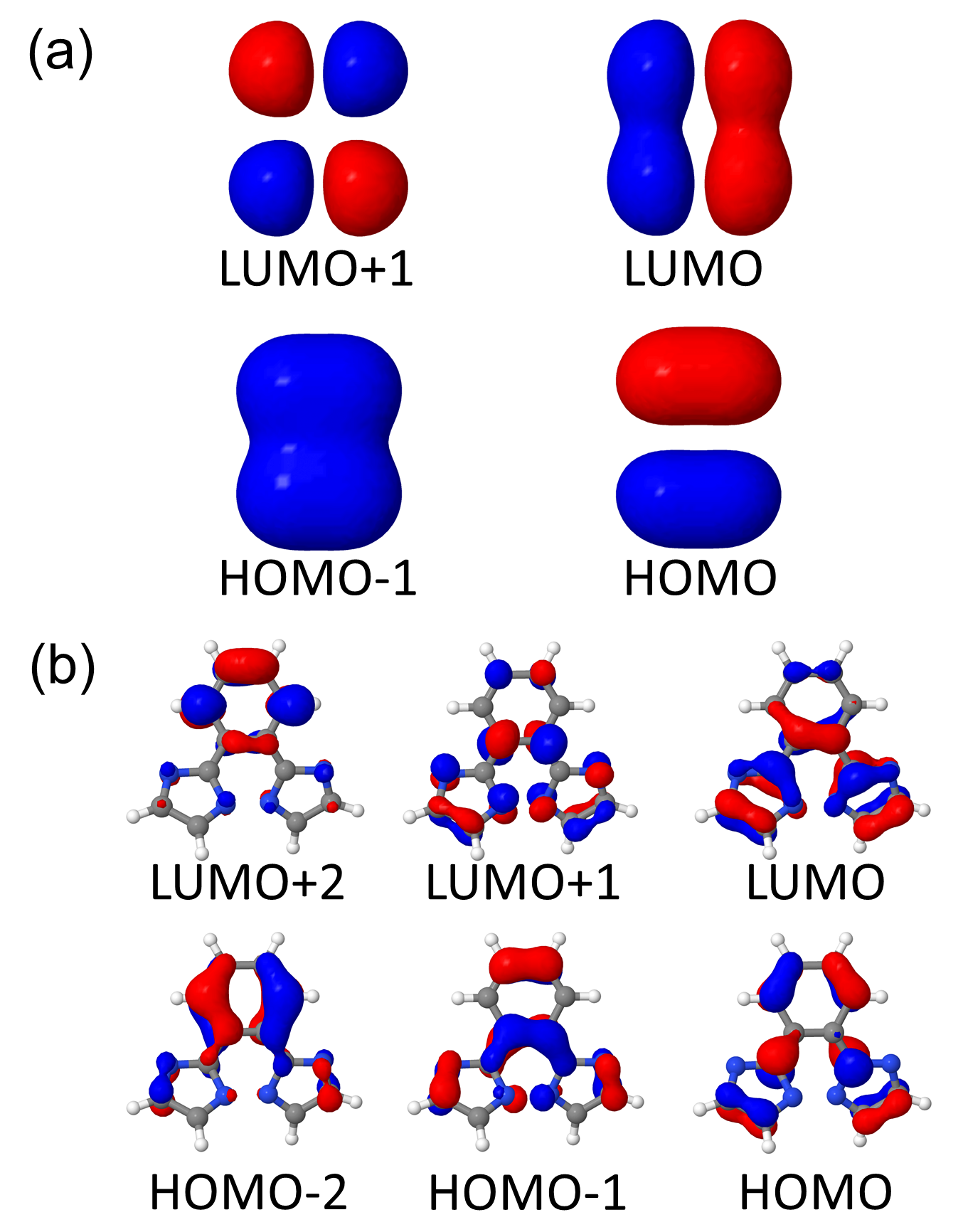
Figure 11: Orbitals for the hydrogen plane model and MABI, where the structures are drawn by Jmol [Jmol_development_team2016-ly]. (a) The orbitals of the hydrogen plane model with ID 2. (b) The orbitals of MABI.

Appendix E Detail of the calculation conditions on VQE and QMC

HTN+QMC codes were implemented by the Python, especially the NumPy [Harris2020-fh] and SciPy [Virtanen2020-rg] packages, and Qiskit [Treinish2023-co] and Qulacs [Suzuki2021-lj] were adopted as quantum circuit simulators. The sequential least squares programming optimizer (SLSQP) in the SciPy package was used in the parameter optimizations. In MABI, although there are six electrons in the ground state in the CASCI(6e,6o) problem, the number of electrons in the ground state of the corresponding qubit Hamiltonian is not six. Thus VQE/AC [Gocho2023-uy] algorithm was used to perform energy optimization with the constraints imposed on the number of electrons. The ground state of MABI refers to the eigenstate with the smallest eigenvalue acquired by restricting the electron number to six.

In all the QMC methods (QMC, QC-QMC, and HTN+QMC), the initial number of walkers was one, and the single reference state was selected as the initial configuration. In the hydrogen plane model (except for ID 3) and MABI, we checked out that the Hartree-Fock state was chosen as the single reference state. The trial wave function was the single reference state, and the states obtained by VQE and HTN+VQE were used for QC-QMC and HTN+QMC, respectively. The maximum number of iterations in all the types of QMC was 10,000.

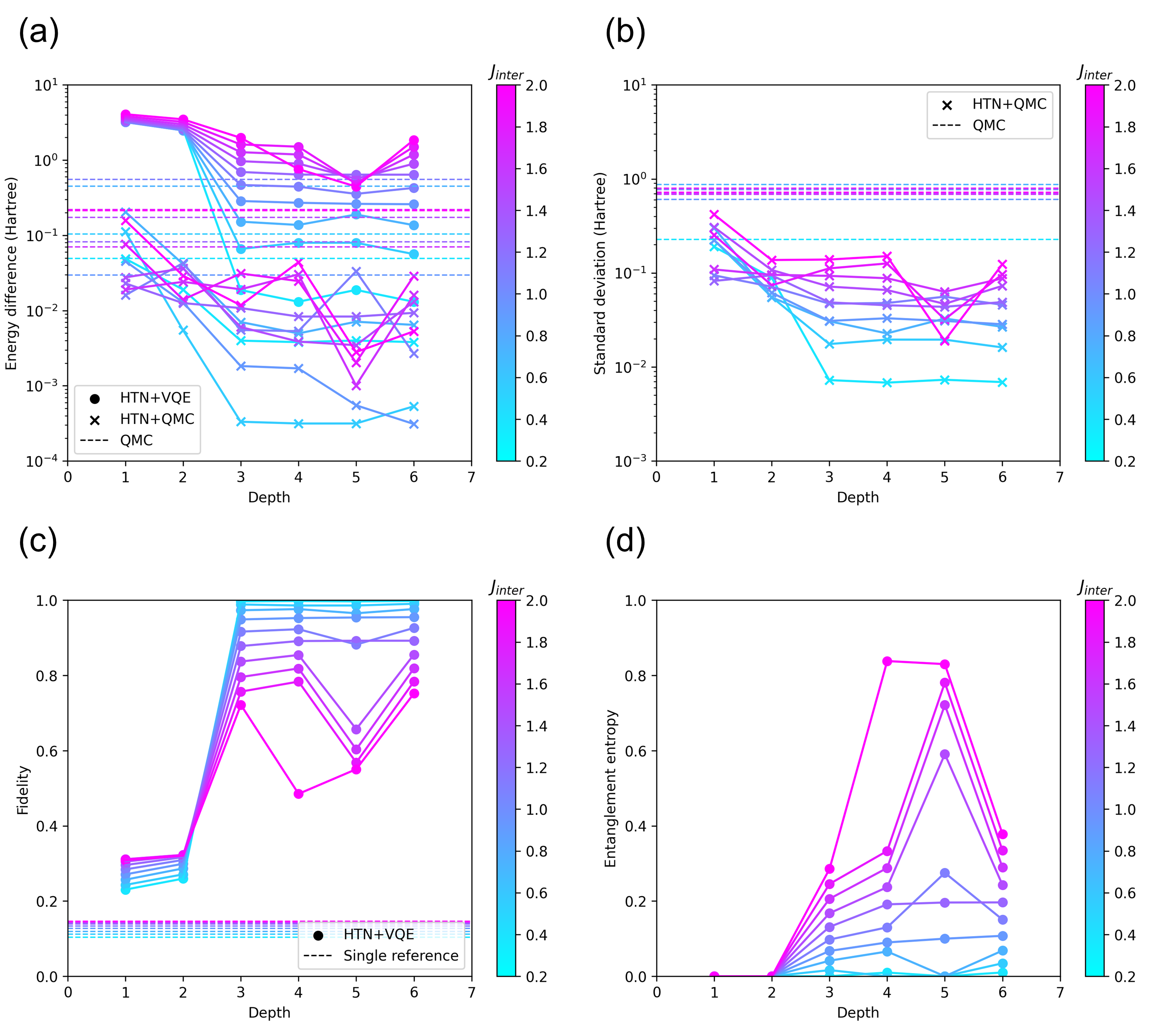
Figure 12: Results of the Heisenberg chain model of the cluster setting with $n=4,k=2$, and $d_{H}=1,2,\dots,6$. The values of $J_{inter}$ are shown in color bars. The circle and cross marks denote the results of HTN+VQE and HTN+QMC, respectively. The dashed lines in (a) and (b) [(c)] denote the results of QMC [a single reference state]. (a) The energy difference. (b) The standard deviation. (c) The fidelity. (d) The bipartite entanglement entropy.

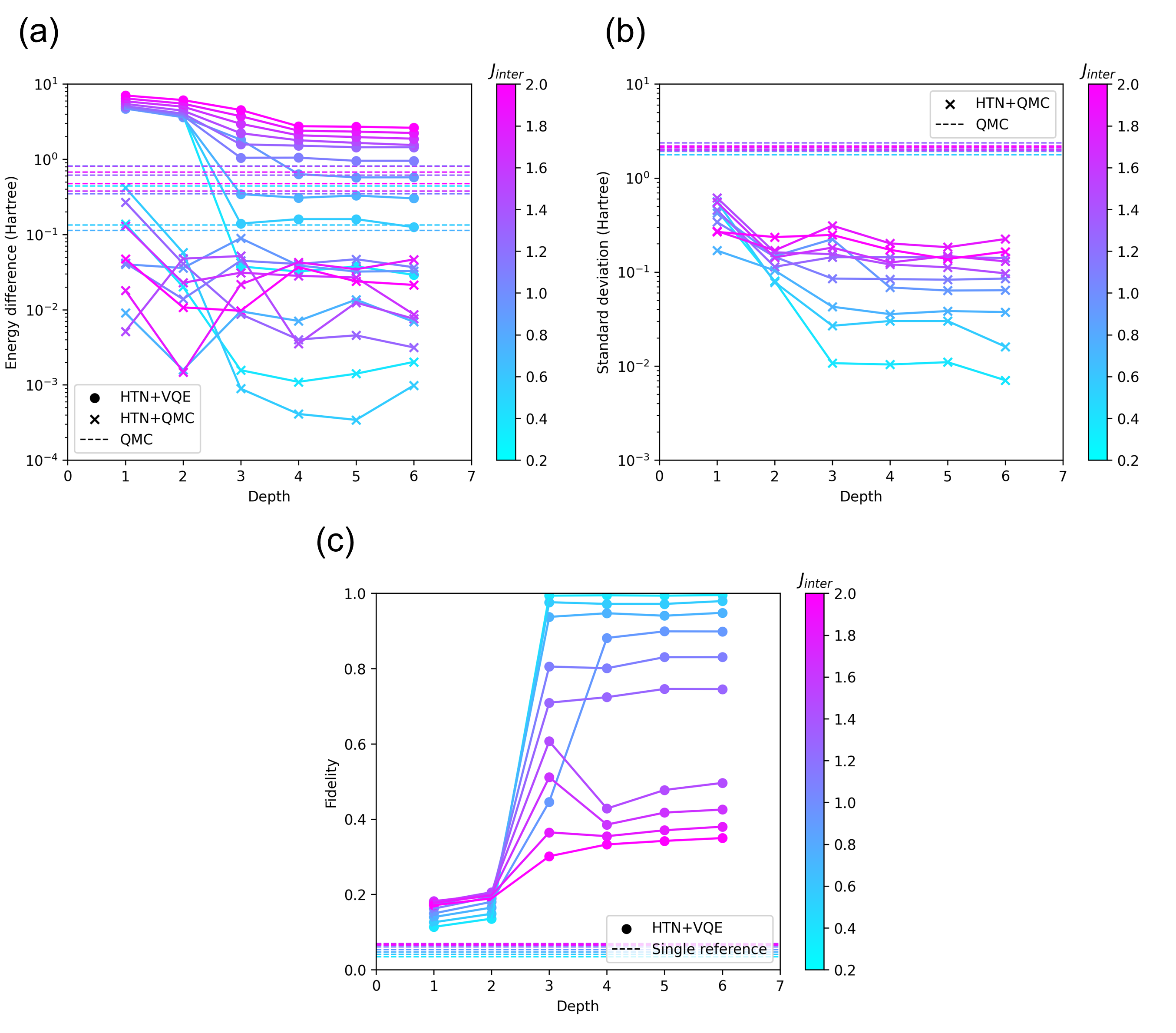
Figure 13: Results of the Heisenberg chain model of the cluster setting with $n=4,k=3$, and $d_{H}=1,2,\dots,6$. The values of $J_{inter}$ are shown in color bars. The circle and cross marks denote the results of HTN+VQE and HTN+QMC, respectively. The dashed lines in (a) and (b) [(c)] denote the results of QMC [a single reference state]. (a) The energy difference. (b) The standard deviation. (c) The fidelity.

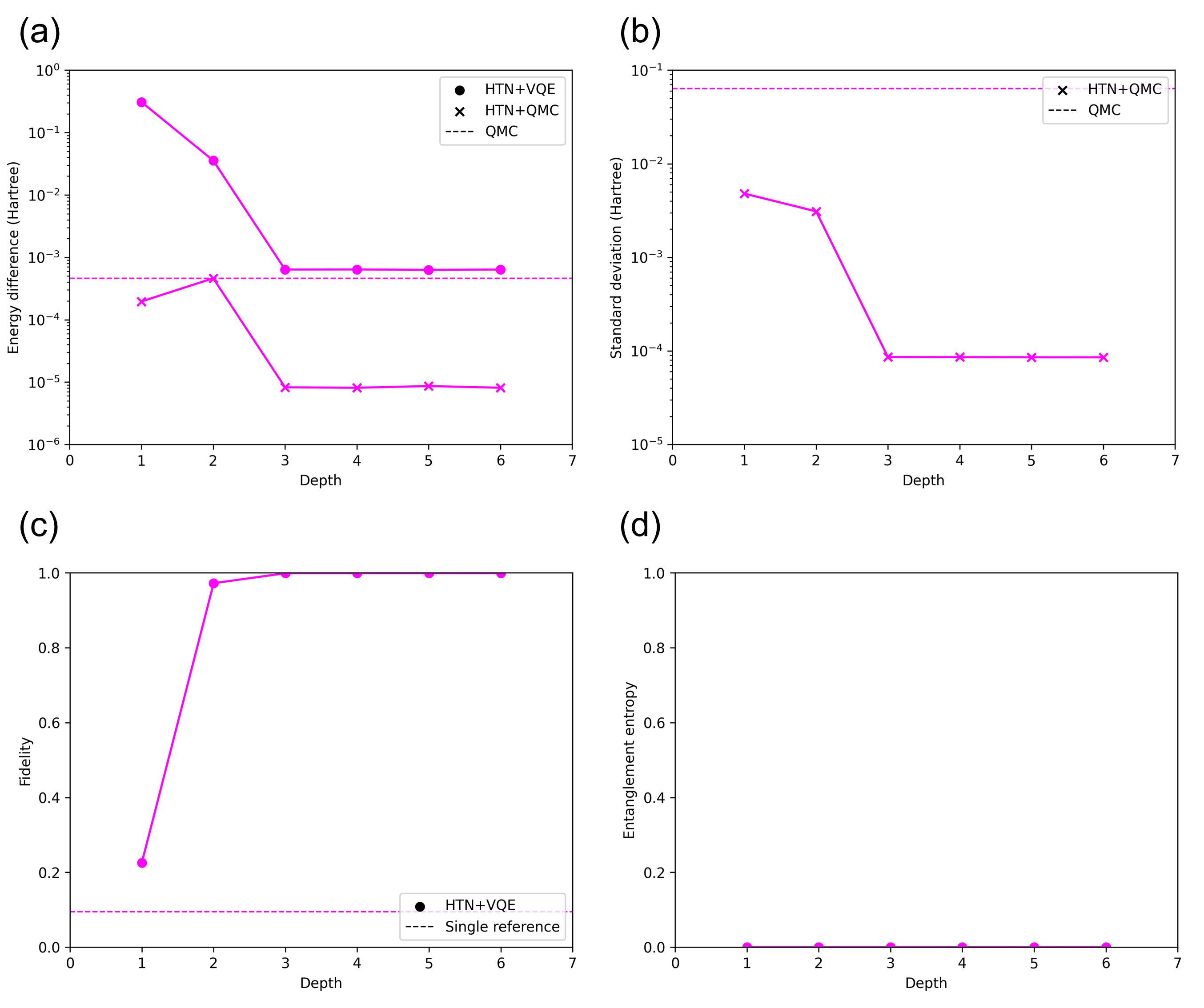
Figure 14: Results of the graphite model of the horizontal setting with $n=4,k=2$, and $d_{H}=1,2,\dots,6$. The circle and cross marks denote the results of HTN+VQE and HTN+QMC, respectively. The dashed lines in (a) and (b) [(c)] denote the results of QMC [a single reference state]. (a) The energy difference. (b) The standard deviation. (c) The fidelity. (d) The bipartite entanglement entropy.

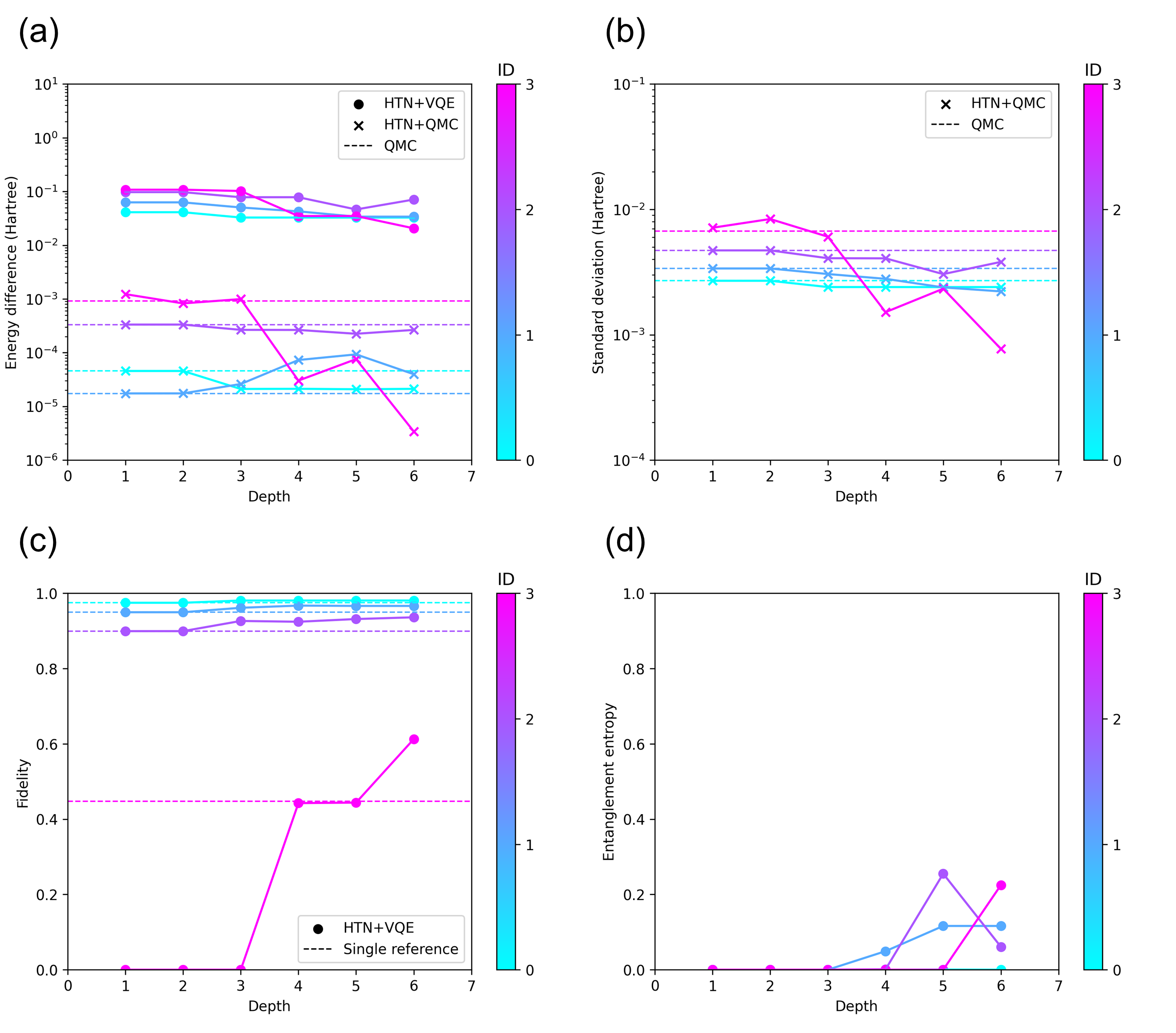
Figure 15: Results of the hydrogen plane model of the HOMO-LUMO setting with $n=4,k=2$, and $d_{H}=1,2,\dots,6$. The values of ID are shown in color bars. The circle and cross marks denote the results of HTN+VQE and HTN+QMC, respectively. The dashed lines in (a) and (b) [(c)] denote the results of QMC [a single reference state]. (a) The energy difference. (b) The standard deviation. (c) The fidelity. (d) The bipartite entanglement entropy.

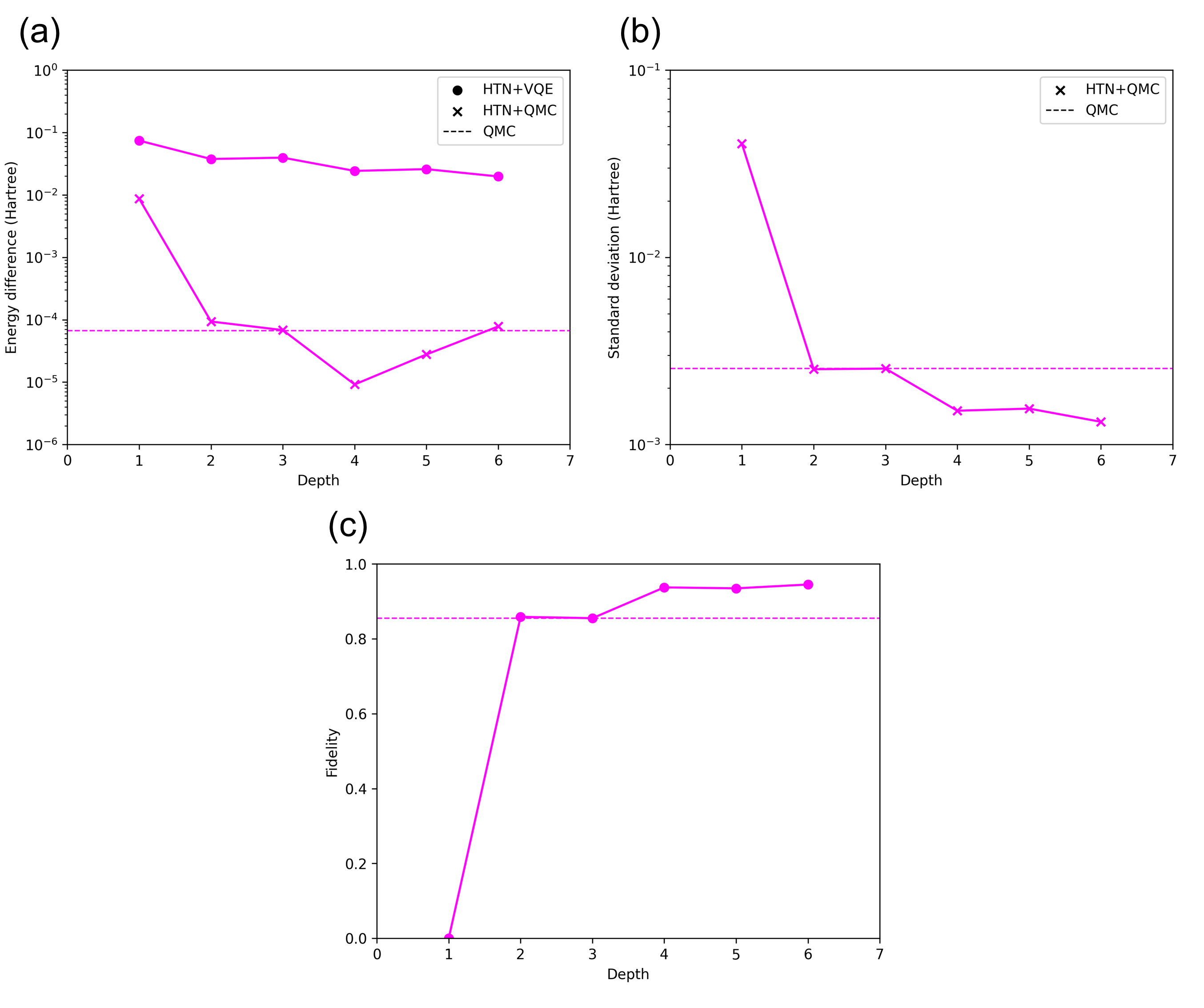
Figure 16: Results of MABI of the HOMO-LUMO setting with $n=4,k=3$, and $d_{H}=1,2,\dots,6$. The circle and cross marks denote the results of HTN+VQE and HTN+QMC, respectively. The dashed lines in (a) and (b) [(c)] denote the results of QMC [a single reference state]. (a) The energy difference. (b) The standard deviation. (c) The fidelity.

Appendix F Benchmark results

We benchmark the models with circuit depth $d_{H}=1,2,\dots,6$. As an example, we first explain the benchmark results of the Heisenberg chain model in the cluster setting with $k=2$, especially $J_{inter}=0.2,1.0$, and $2.0$ Hartree. Figure 12(a), (b), and (c) show the energy difference, standard deviation, and fidelity versus circuit $d_{H}$, respectively. For HTN+VQE in Fig. 12(a), on the one hand, the energy difference is more than $10^{-1}$ Hartree when $J_{inter}$ is large, e.g., for $J_{inter}=1.0$ Hartree, the difference is $4.3\times 10^{-1}$ Hartree even with $d_{H}=6$. On the other hand, all the values of the difference for HTN+QMC are less than $10^{-1}$ Hartree with $d_{H}\geq 2$. In addition, the difference for HTN+QMC with $d_{H}\geq 3$ is more than one order of magnitude less than that of QMC. In Fig. 12(b), the decrease in the standard deviation from QMC is also confirmed in HTN+QMC. From the results, we find that HTN+QMC can evaluate the energy more accurately than the previous classical and quantum algorithms.

Figure 12(c) shows the fidelity of HTN+VQE, and the fidelity for the single reference state used as the QMC trial wave function is also shown. The energy accuracy worsens as the fidelity decreases, for example of $d_{H}=4$, the fidelity with $J_{inter}=0.2,1.0$, and $2.0$ Hartree is 1.00, 0.92, and 0.49, respectively, and the energy difference with $J_{inter}=2.0$ for HTN+QMC in Fig. 12(a) is one order of magnitude larger than that of $J_{inter}=0.2$ and 1.0. Nevertheless, the energy difference with $d_{H}=4$ and $J_{inter}=2.0$ for HTN+QMC is one order of magnitude less than that for QMC, i.e., the accuracy of HTN+QMC is still higher than that of QMC even when the fidelity is low. Therefore, even if the trial wave function prepared in HTN+VQE is not highly accurate, HTN+QMC can be expected to provide better energy accuracy than the classical calculation. Note that we also calculate the bipartite entropy for the models in Fig. 12(d), which tends to increase with $J_{inter}$.

Finally, we show the benchmark results for the Heisenberg chain model with $k=3$, the graphite model, the hydrogen plane model, and MABI as in Figs. 13, 14, 15, and 16, respectively. The results of bipartite entanglement entropy are shown for the models with $k=2$. From these data, we determined that $d_{H}=4$ would provide sufficient accuracy and adopted this value as the default.

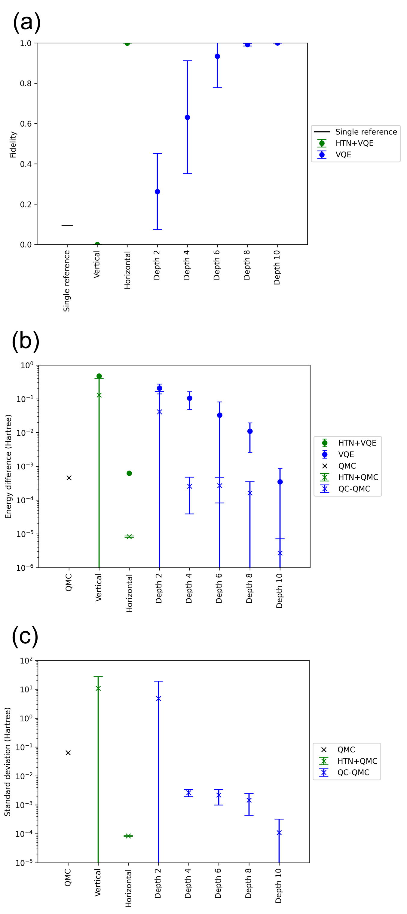
Figure 17: Results of the analysis for the graphite model. The average values and error bars were calculated over 10 different random seeds used for the initial parameters in VQE or HTN+VQE execution. For reference, values obtained from the single reference state and those from QMC are shown by the black bar in (a) and cross in (b) and (c), respectively. The green (blue) circle and cross denote the results from the decomposition (no-decomposition) setting in HTN+VQE and HTN+QMC (VQE and QC-QMC), respectively. In HTN+VQE and HTN+QMC, $n=4$ and $k=2$ for all the settings. (a) The fidelity. (b) The energy difference. (c) The standard deviation.

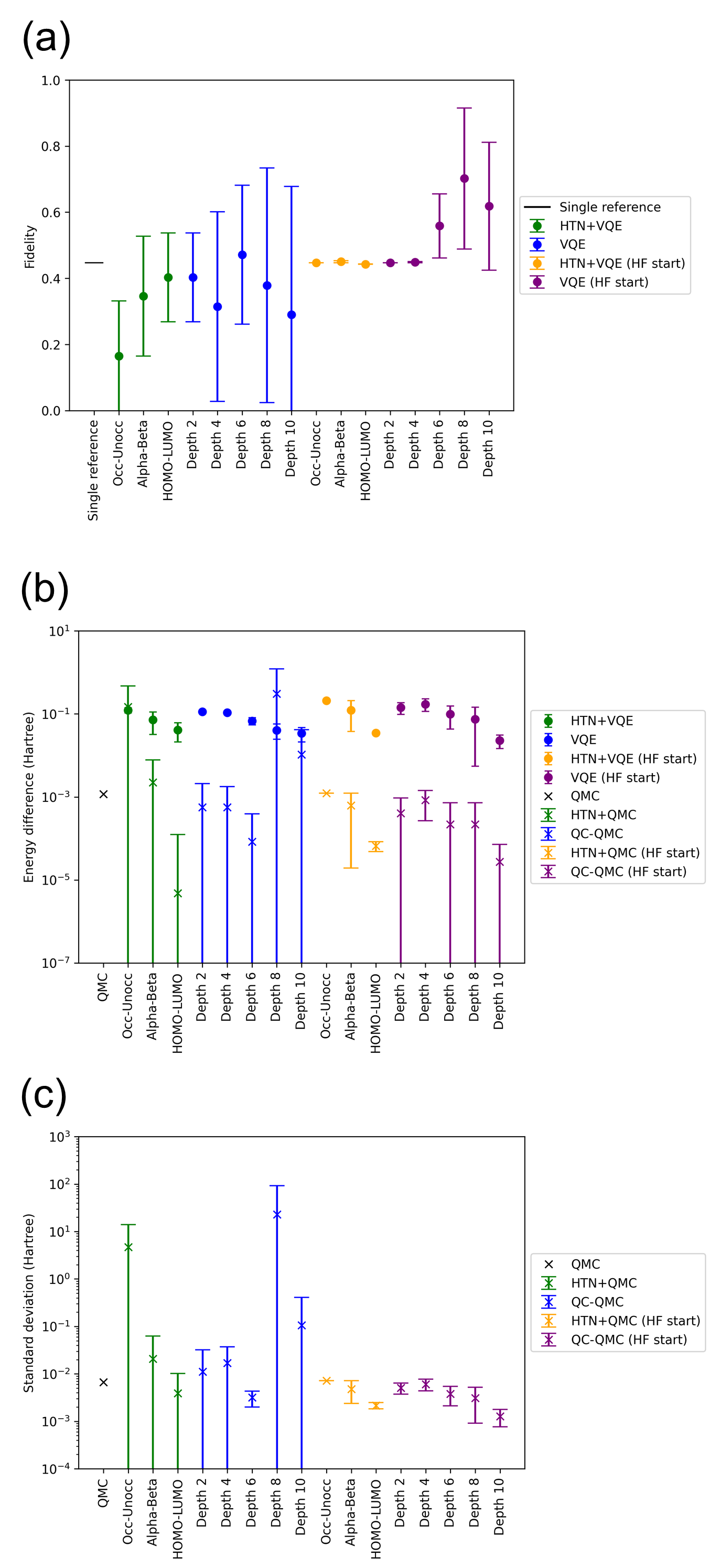
Figure 18: Results of the analysis for the hydrogen plane model with ID 3. The average values and error bars were calculated over 10 different random seeds used for the initial parameters in VQE or HTN+VQE execution. For reference, values obtained from the single reference state and those from QMC are shown by the black bar in (a) and cross in (b) and (c), respectively. The green circle, green cross, blue circle, and blue cross respectively denote the results from the decomposition, decomposition, no-decomposition, and no-decomposition settings in HTN+VQE, HTN+QMC, VQE, and QC-QMC, and the yellow circle, yellow cross, purple circle, and purple cross respectively denote those when the initial state is close to the Hartree-Fock state in HTN+VQE, HTN+VQE, VQE, and VQE. In HTN+VQE and HTN+QMC, $n=4$ and $k=2$ for all the settings. (a) The fidelity. (b) The energy difference. (c) The standard deviation.

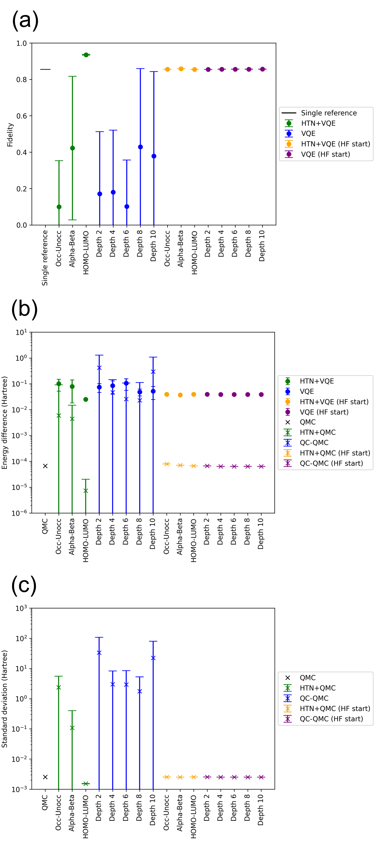
Figure 19: Results of the analysis for MABI. The average values and error bars were calculated over 10 different random seeds used for the initial parameters in VQE or HTN+VQE execution. For reference, values obtained from the single reference state and those from QMC are shown by the black bar in (a) and cross in (b) and (c), respectively. The green circle, green cross, blue circle, and blue cross respectively denote the results from the decomposition, decomposition, no-decomposition, and no-decomposition settings in HTN+VQE, HTN+QMC, VQE, and QC-QMC, and the yellow circle, yellow cross, purple circle, and purple cross respectively denote those when the initial state is close to the Hartree-Fock state in HTN+VQE, HTN+VQE, VQE, and VQE. In HTN+VQE and HTN+QMC, $n=4$, $k=3$ for the HOMO-LUMO setting, and $n=6$, $k=2$ for the other two settings. (a) The fidelity. (b) The energy difference. (c) The standard deviation.

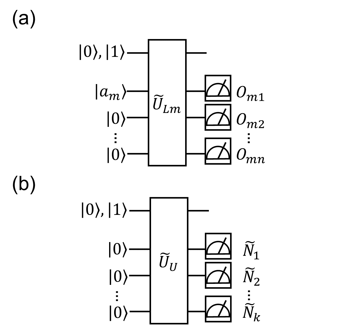
Figure 20: Quantum circuits for calculating HTN+VQE to execute the pseudo-Hadamard test. The topmost line represents an ancilla qubit and the other lines represent system qubits. The circuit with the ancilla qubit set to $\ket{0}$ is used when calculating constraints. (a) The calculation for the lower tensor. (b) The calculation for the upper tensor.

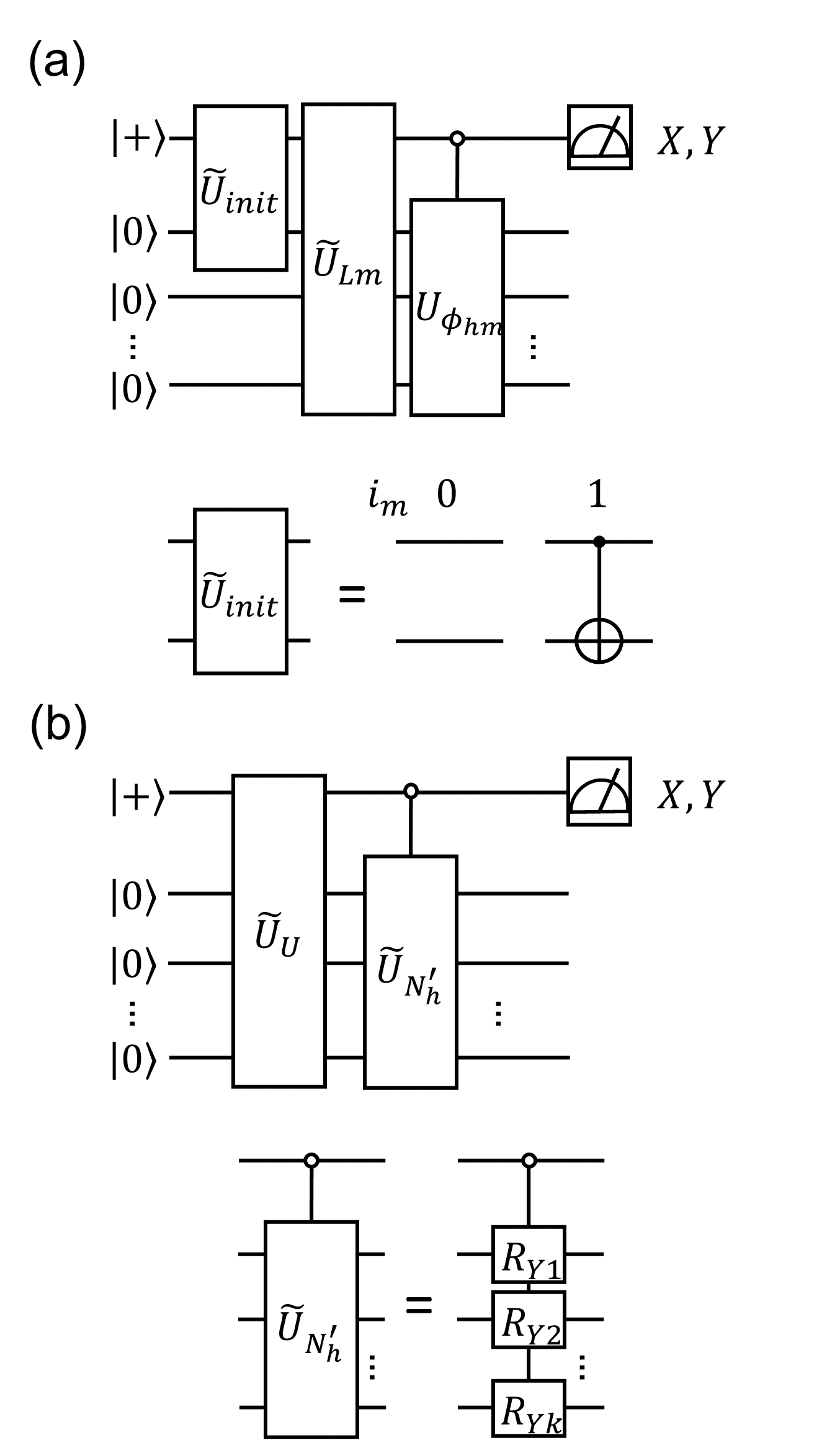
Figure 21: Quantum circuits for calculating $T_{h}$ by using pseudo-Hadamard test. The topmost line represents an ancilla qubit and the other lines represent system qubits. (a) The calculation for the lower tensor. (b) The calculation for the upper tensor.

Appendix G Remaining results of the decomposition settings

We discuss the results of the Heisenberg chain model with $k=2$ and $J_{inter}=1.0$, the graphite model, the hydrogen plane model with ID 3, and MABI. Table 3 show the values of $G_{mr}$ defined in Eq. (9) and the mutual information. The mutual information for two and three subsystems $I(A;B)$ and $I(A;B;C)$ are defined as

$$I(A;B)=H(A)+H(B)-H(A,B),$$ (35)

and

$$I(A;B;C)=I(A;B)-I(A;B|C),$$ (36)

respectively, where $I(A;B|C)=I(A|C)-I(A|B,C),I(A|C)=H(C,A)-H(C),I(A|B,C)=H(B,C,A)-H(B,C)$, and $H(A)$ is von Neumann entropy calculated from the reduced density matrix for the subsystem $A$. We transformed the wave function, which was originally constructed in an NumPy array to the reduced density matrix using PennyLane [Bergholm2018-cn].

Figures 18, 18, and 19 show the results of the analysis for the graphite model, the hydrogen plane model with ID 3, and MABI, respectively. We also executed the VQE and HTN+VQE using the initial state close to the Hartree-Fock state; the unitary matrix $U$ corresponding to the real amplitude ansatz with all parameters set to zero satisfies $U\ket{0}^{\otimes nk}=\ket{0}^{\otimes nk}$, and thus an arbitrary basis state (including Hartree-Fock state) $\ket{\phi_{h}}$ can be constructed in the state preparation for VQE by applying Pauli $X$ gates on the appropriate qubits after $U$. In the following, we show that the same state construction is also possible in HTN+VQE. In case that the basis state corresponds to a computational basis state $\ket{\phi_{h}}=\bigotimes_{m,r}\ket{j_{mr}(h)}=(\bigotimes_{m,r}X^{j_{mr}(h)})\ket{0}^{\bigotimes nk}$, the state can be constucted by substituting $U_{Lm}$ for $\bigotimes_{r}X^{j_{mr}(h)}U_{Lm}$ in HTN, where $j_{mr}(h)\in\{0,1\}$: assuming $\ket{\varphi^{i_{m}}}=\bigotimes_{r}X^{j_{mr}(h)}U_{Lm}\ket{i_{m}}\ket{0}^{\otimes n-1}$, $\psi_{\vec{i}}=\matrixelement{\vec{i}}{U_{U}}{0}^{\otimes k}$, $U_{Lm}\ket{0}^{\otimes n}=\ket{0}^{\otimes n}$, and $U_{U}\ket{0}^{\otimes k}=\ket{0}^{\otimes k}$, $\ket{\psi_{HTN}}$ in Eq. (19) becomes

$$\ket{\psi_{HTN}} =\sum_{\vec{i}}\psi_{\vec{i}}\bigotimes_{m}\ket{\varphi^{i_{m}}}$$ (37)

$$=\bigotimes_{m}\ket{\varphi^{0}}$$

$$=(\bigotimes_{m,r}X^{j_{mr}(h)})\ket{0}^{\otimes nk}.$$

We performed the VQE and HTN+VQE from the initial states close to the Hartree-Fock state by using the initial parameters which are chosen randomly from $[0,0.01)$, and the results for the hydrogen plane model with ID 3 and MABI are shown in Figs. 18 and 19, respectively.

Table 3: Values of $G_{mr}$ and mutual information (MI) in all the decomposition settings. The “Decomposition” column represents the decomposition setting for the models. $k$ denotes the number of subsystems. The unit of $G_{mr}$ is Hartree.

Model	Decomposition	$k$	$G_{mr}$	MI
Heisenberg	Cluster	2	1.50	1.32
	Even-Odd	2	10.50	6.92
Graphite	Horizontal	2	0.02	0.03
	Vertical	2	0.65	7.85
Hydrogen plane	HOMO-LUMO	2	1.51	1.14
	Alpha-Beta	2	1.65	2.84
	Occ-Unocc	2	1.44	3.14
MABI	HOMO-LUMO	3	1.67	0.00
	Alpha-Beta	2	1.96	0.68
	Occ-Unocc	2	2.10	1.33

Appendix H Details of real device procedure

We describe the algorithm for overlap calculation modified for executing HTN on real devices by using the pseudo-Hadamard test, in addition to the theoretical analysis on noise resilience.

H.1 Extension of the pseudo-Hadamard test to HTN

We start with the wave function involving the ancilla qubit

$$\ket{\tilde{\psi}_{HTN}}=\sum_{\vec{i}}\tilde{\psi}_{\vec{i}}\bigotimes_{m}\ket{\tilde{\varphi}^{i_{m}}}.$$ (38)

Based on the ansatz shown in Fig. 4(b), the variational formulation of this wave function is

$$\underset{\tilde{U}_{Lm},\tilde{U}_{U}}{\min} \expectationvalue{H}{\tilde{\psi}_{HTN}}$$ (39)

s.t. $$\expectationvalue{n_{Lm}}=0\quad\forall m\in\{1,2,\dots,k\},$$

$$\expectationvalue{n_{U}}=0,$$

where

$$\expectationvalue{n_{Lm}}$$ (40)

$$=\bra{0}\bra{0}^{\otimes n}\tilde{U}_{Lm}^{{\dagger}}(\sum_{r=1}^{n}I^{\otimes r}\otimes n_{mr}\otimes I^{\otimes n-r})\tilde{U}_{Lm}\ket{0}\ket{0}^{\otimes n}$$

$$\expectationvalue{n_{U}}$$

$$=\bra{0}\bra{0}^{\otimes k}\tilde{U}_{U}^{{\dagger}}(\sum_{m=1}^{k}I^{\otimes m}\otimes n_{m}\otimes I^{\otimes k-m})\tilde{U}_{U}\ket{0}\ket{0}^{\otimes k},$$

$\tilde{U}_{Lm}$ and $\tilde{U}_{U}$ are unitary gates that are specified in detail in the next paragraph.

The expectation value of the observable can be rewritten in terms of the upper and lower tensors (both involving the ancilla) as

$$\expectationvalue{O}{\tilde{\psi}_{HTN}}$$ (41)

$$=\sum_{\vec{i^{\prime}}~{}\vec{i}}\tilde{\psi}_{\vec{i^{\prime}}}^{*}\tilde{\psi}_{\vec{i}}\prod_{m=1}^{k}\matrixelement{\tilde{\varphi}^{i_{m}^{\prime}}}{\bigotimes_{r=1}^{n}O_{mr}}{\tilde{\varphi}^{i_{m}}}$$

$$=\sum_{\vec{i^{\prime}}~{}\vec{i}}\tilde{\psi}_{\vec{i^{\prime}}}^{*}\tilde{\psi}_{\vec{i}}\prod_{m=1}^{k}\bra{1}\bra*{\tilde{\varphi}^{i_{m}^{\prime}}}(I\otimes\bigotimes_{r=1}^{n}O_{mr})\ket{1}\ket*{\tilde{\varphi}^{i_{m}}}$$

$$=\sum_{\vec{i^{\prime}}~{}\vec{i}}\tilde{\psi}_{\vec{i^{\prime}}}^{*}\tilde{\psi}_{\vec{i}}\prod_{m=1}^{k}\tilde{N}^{i_{m}^{\prime}i_{m}}.$$

Figure 20(a) show the quantum circuit for calculating $\tilde{N}^{i_{m}^{\prime}i_{m}}$ in the lower tensor assuming $\ket{1}\ket{\tilde{\varphi}^{i_{m}}}=\tilde{U}_{Lm}\ket{1}\ket{i_{m}}\ket{0}^{\otimes n-1}$. We construct $\tilde{N}_{m}=\matrixquantity(\tilde{N}^{00}&\tilde{N}^{01}\\ \tilde{N}^{10}&\tilde{N}^{11})$ by combining the results from the lower tensors for the four initial states; $\ket{a_{m}}$ takes $\ket{0},\ket{1},\ket{+},$ and $\ket{y+}$, and from the corresponding measurement results denoted by $M^{0},M^{1},M^{+},$ and $M^{y+}$, respectively, we obtain the matrix elements $\tilde{N}^{00}=M^{0},\tilde{N}^{11}=M^{1},\tilde{N}^{01}=\frac{i-1}{2}M^{0}+\frac{i-1}{2}M^{1}+M^{+}-iM^{y+},$ and $\tilde{N}^{10}=\tilde{N}^{01*}$ [Kanno2021-zn]. Eq. (42) then becomes the evaluation in the upper tensor

$$\expectationvalue{O}{\tilde{\psi}_{HTN}} =\expectationvalue{\bigotimes_{m=1}^{k}\tilde{N}_{m}}{\tilde{\psi}}$$ (42)

$$=\bra*{1}\bra*{\tilde{\psi}}(I\otimes\bigotimes_{m=1}^{k}\tilde{N}_{m})\ket*{1}\ket*{\tilde{\psi}}$$

Figure 20(b) shows the circuit for calculating the last expression assuming $\ket*{1}\ket*{\tilde{\psi}}=\tilde{U}_{U}\ket*{1}\ket*{0}^{\otimes k}$. Alternatively, $\tilde{N}_{m}$ is Hermitian and can be measured using the eigenvalue decomposition of $\tilde{N}_{m}$ classically.

Now we move on to the overlap $T_{h}$ between the quantum state and standard basis state, which is represented similarly to the observable as

$$T_{h} =\innerproduct{\tilde{\psi}_{HTN}}{\phi_{h}}$$ (43)

$$=\sum_{\vec{i}}\tilde{\psi}_{\vec{i}}^{*}\prod_{m=1}^{k}\innerproduct{\tilde{\varphi}^{i_{m}}}{\phi_{hm}}$$

$$=\sum_{\vec{i}}\tilde{\psi}_{\vec{i}}^{*}\prod_{m=1}^{k}\tilde{N}^{i_{hm}}$$

The circuit for calculating $\tilde{N}^{i_{hm}}$ in the lower tensor is shown in Fig. 21(a). Since there is no tensor index in $\ket{\phi_{hm}}$, only two different circuits are needed for $\tilde{U}_{init}$ (the lower panel of the figure). $U_{\phi_{hm}}$ is composed of CNOT gates from ancilla to target qubits, which should be set to $\ket{1}$ in $\ket{\phi_{hm}}$. Next, we explain the calculation of the upper tensor. $\tilde{N}^{i_{hm}}$ is a tensor with one leg, i.e., can be represented using a two-element vector as $\tilde{N}^{i_{hm}}=\innerproduct{i_{m}}{\tilde{N}_{hm}}$. $T_{h}$ is then written as

$$T_{h} =\sum_{\vec{i}}\tilde{\psi}_{\vec{i}}^{*}\prod_{m=1}^{k}\innerproduct{i_{m}}{\tilde{N}_{hm}}$$ (44)

$$=\sqrt{\prod_{m=1}^{k}\innerproduct{\tilde{N}_{hm}}{\tilde{N}_{hm}}}\innerproduct{\tilde{\psi}}{\tilde{N}^{{}^{\prime}}_{h}},$$

where

$$\ket{\tilde{N}^{{}^{\prime}}_{h}} =\bigotimes_{m=1}^{k}\ket{\tilde{N}^{{}^{\prime}}_{hm}}$$ (45)

$$=\bigotimes_{m=1}^{k}\frac{\ket{\tilde{N}_{hm}}}{\sqrt{\innerproduct{\tilde{N}_{hm}}{\tilde{N}_{hm}}}}$$

$$=\matrixquantity(\alpha_{hm}\\ \beta_{hm}),$$

$\sqrt{\prod_{m=1}^{k}\innerproduct{\tilde{N}_{hm}}{\tilde{N}_{hm}}}$ is a normalization constant, and $\alpha_{hm}^{2}+\beta_{hm}^{2}=1$. The circuit for the upper tensor is shown in Fig. 21(b), where $\ket{\tilde{N}^{{}^{\prime}}_{h}}$ is embedded by using controlled-RY gates (lower panel of the figure). The rotation angle of $R_{Ym}$ is set to $\theta_{hm}=2\mathrm{arccos}(\alpha_{hm})$, and is substituted for $-\theta_{hm}$ if $\beta_{hm}<0$. Note that ancilla qubits are measured only $X$ basis in this study since the trial wave function is real.

Finally, the rest of the calculation conditions, which are not described in Sec. II.1, are listed below. We checked on the four-qubit Heisenberg chain model to confirm that the amplitudes close to those of the exact ground state were obtained by using the pseudo-Hadamard test when a highly accurate wave function is obtained in HTN+VQE. We used at most five qubits in real device execution, where the initial layout in the device was $[12,15,18,21,23]$, and the number of shots was 4000. We combined the constraints in Eq. (LABEL:eq:_HTN+VQE_with_constraint) as $\sum_{m}\expectationvalue{n_{Lm}}+\expectationvalue{n_{U}}=0$ in the implementation since the left side of each constraint in Eq. (LABEL:eq:_HTN+VQE_with_constraint) is non-negative for any $\tilde{U}_{Lm}$ and $\tilde{U}_{U}$ because they consists of the expectation values for the particle number. The overlaps are calculated only for the Slater determinants of four and six electrons in the hydrogen plane model and MABI, respectively, with the rest of the amplitudes set to zeros. In the calculation of MABI, in addition to the constraints on the overlap calculation, an additional constraint enforcing the number of electrons to be six was imposed.

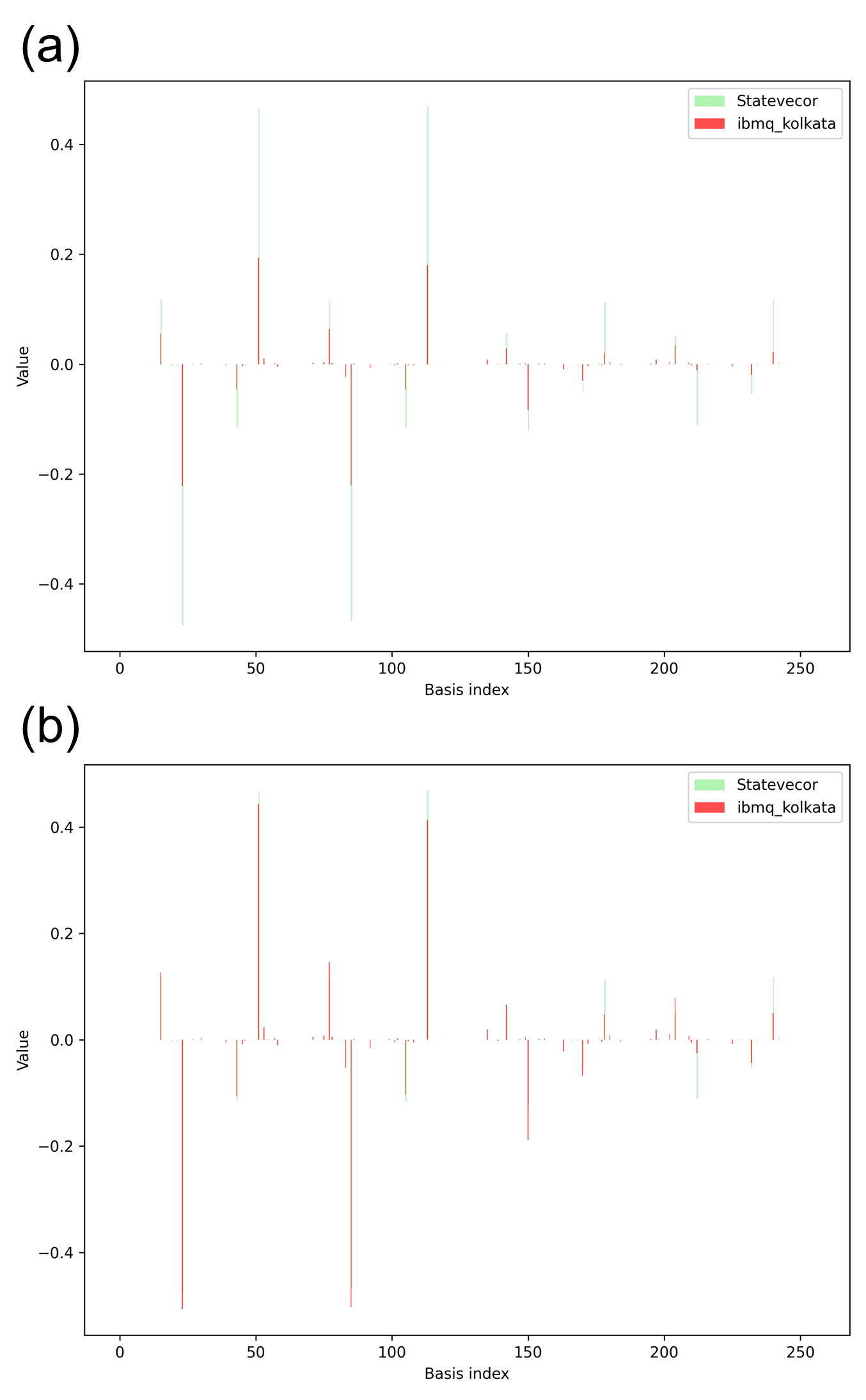
Figure 22: Results of $T_{h}$ in the hydrogen plane model without and with normalization in the real device procedure. The light green and red bars represent the values in the statevector and real device procedure, respectively. (a) The result without normalization. (b) The result with normalization.

H.2 Analysis of noise resilience

We discuss the reason for the robustness of HTN+QMC to the noise. In the circuit of Fig. 7(b), the state before the measurement $\rho$ is represented as

$$\rho =\ket{\lambda}\bra{\lambda},$$ (46)

$$\ket{\lambda} =\frac{1}{\sqrt{2}}(\ket{0}\ket{\phi_{h}}+\ket{1}\ket*{\tilde{\psi}}).$$

When a depolarizing channel applies to $\rho$, i.e., $\rho^{\prime}=(1-p)\rho+pI^{\otimes n_{s}+1}$ where $p$ is an error rate, the expectation value after the measurement is given

$$\mathrm{Tr}((X\otimes I^{\otimes n_{s}})\rho^{\prime}) =(1-p)\innerproduct{\tilde{\psi}}{\phi_{h}}$$ (47)

$$+p\mathrm{Tr}((X\otimes I^{\otimes n_{s}})I^{\otimes n_{s}+1}))$$

$$=(1-p)\innerproduct{\tilde{\psi}}{\phi_{h}}.$$

Since $T_{h}$ can be represented by substituting $\tilde{U}_{\psi}=(\prod_{m}\tilde{U}_{Lm})\tilde{U}_{U}$, $U_{\phi_{h}}=\prod_{m}U_{\phi_{hm}}$, and $n_{s}=nk$ in Fig. 7(b), we can assume the above discussion holds true, where $\tilde{U}_{Lm}$ operates the ancilla qubit and qubits corresponding to $m$-th subsystem, and $\tilde{U}_{U}$ operates on the ancilla qubit and qubits corresponding the first qubit of each subsystem. Then the ratio of $T_{h}$ for different standard basis states is

$$\frac{T_{h}}{T_{h}^{\prime}} =\frac{(1-p)\innerproduct{\tilde{\psi}_{HTN}}{\phi_{h}}}{(1-p)\innerproduct{\tilde{\psi}_{HTN}}{\phi_{h^{\prime}}}}$$ (48)

$$=\frac{\innerproduct{\tilde{\psi}_{HTN}}{\phi_{h}}}{\innerproduct{\tilde{\psi}_{HTN}}{\phi_{h^{\prime}}}}.$$

Since $E_{mix}$ is an estimator that includes the normalization of the wave function in HTN, HTN+QMC is unaffected by depolarizing noise. Figure 22(a) and (b) show the results of $T_{h}$ in the hydrogen plane model without and with the normalization, respectively. The fidelity is restored from 0.09 to 0.49 through normalization, whereas the fidelity is 0.46 in the statevector. As a result, the noise robustness of HTN+QMC, which was experimentally observed, was supported theoretically and numerically.