Differentially Private Stream Processing at Scale

Abstract

We design, to the best of our knowledge, the first differentially private (DP) stream processing system at scale. Our system – Differential Privacy SQL Pipelines (DP-SQLP) – is built using a streaming framework similar to Spark streaming, and is built on top of the Spanner database and the F1 query engine from Google.

Towards designing DP-SQLP we make both algorithmic and systemic advances, namely, we (i) design a novel DP key selection algorithm that can operate on an unbounded set of possible keys, and can scale to one billion keys that users have contributed, (ii) design a preemptive execution scheme for DP key selection that avoids enumerating all the keys at each triggering time, and (iii) use algorithmic techniques from DP continual observation to release a continual DP histogram of user contributions to different keys over the stream length. We empirically demonstrate the efficacy by obtaining at least $16\times$ reduction in error over meaningful baselines we consider.

1 Introduction

Analysis of streaming data with differential privacy (DP) [16] has been studied from the initial days of the field [17, 11], and this has been followed up in a sequence of works that include computing simple statistics [37], to machine learning applications (a.k.a. online learning) [26, 40, 2, 27, 49]. While all of these works focus on the abstract algorithmic design for various artifacts of streaming data processing, to the best of our knowledge, none of them focus on designing a scalable stream processing system. In this work, we primarily focus on designing a scalable DP stream processing system, called Differential Privacy SQL Pipelines (DP-SQLP), and make algorithmic advances along the way to cater to the scalability needs of it. DP-SQLP is implemented using a streaming framework similar to Spark streaming [48], and is built on top of the Spanner database [13] and F1 query engine [39] from Google.

In this paper we consider a data stream to be an unbounded sequence of tuples of the form $(\texttt{key}\,,$ $\texttt{value}\,,$ $\texttt{timestamp}\,,$ $\texttt{user\_id}\,)$ that gets generated continuously in time. We also have a discrete set of times (a.k.a. triggering times) $\texttt{Tr}=[t^{\sf tr}_{1},t^{\sf tr}_{2},...,t^{\sf tr}_{T}]$. The objective is to output the sum of all the values for each of the keys at each time $t^{\sf tr}_{i}$, while preserving $(\varepsilon,\delta)$-DP [16] over the entire output stream with respect to all of the contributions with the same user_id . Although prior research has extended simple one-shot DP algorithms to the streaming setting [17, 11, 10], designing an at-scale DP-streaming system using off-the-shelf algorithms is challenging because of the following reasons:

1. Unknown key space: A data stream processing system can only process the data that has already arrived. For example, keys for a GROUP BY  operation are not known in advance; instead we discover new keys as they arrive. To ensure $(\varepsilon,\delta)$-DP one has to ensure the set of keys for which the statistics are computed is stable to change of an individual user’s data. That is, we can only report statistics for a particular key  when enough users have contributed to it; to ensure DP the threshold for reporting a key must be randomized.

2. Synchronous execution: The execution of the streaming system is driven by the data stream. That is, we must process the data as it arrives, and cannot run asynchronously at times when there is nothing to trigger execution. We refer to the times when our system runs as triggering times. Furthermore, typically, at each triggering time, only the keys that appeared since the last triggering time are processed. However, this is problematic for DP – if we only output a key when it has appeared in the most recent event time window, then this potentially leaks information. Naively, to avoid this, one has to process all the keys at each triggering time, which is computationally prohibitive.

3. Large number of observed keys and events: A fundamental challenge is scalability. The system should be able to handle millions of updates per second from a data stream with billions of distinct keys.

4. Effective user contribution bounding: In real applications, each person may contribute multiple records to the data stream at different times. Providing “event-level DP” (where a single action by a person/user is protected) does not provide sufficient privacy protection. In this work, we provide “user-level DP”, where all the actions by a person/user is protected simultaneously. To provide user-level DP, one has to bound the contribution of each user, and that eventually introduces bias on the statistics that get computed. But contribution bounding controls the variance of the noise we must add to ensure DP. A natural (and unavoidable [5, 34, 29]) challenge is to decide on the level of contribution bounding to balance this bias and variance.

5. Streaming release of statistics: One has to output statistics at every triggering time. If we treat each triggering time as an independent DP data release, then the privacy cost grows rapidly with the number of releases. Alternatively, to attain a fixed DP guarantee, the noise we add at each triggering time must grow polynomially with the number of triggering times. This is impractical when the number of triggering times is large. Thus the noise we add to ensure DP is not independent across triggering times. This helps in drastically reducing the total noise introduce for a fixed DP guarantee.

In our design of DP-SQLP we address these challenges, either by designing new algorithms, or by implementing existing specialized algorithms. This is our main contribution. To the best of our knowledge, we provide the first at-scale differentially private distributed stream processing system.

Motivation for DP-SQLP: Data streams appear commonly in settings like Web logs, spatio-temporal GPS traces [6], mobile App usages [31], data generated by sensor networks and smart devices [33], live traffic in maps [46], cardiovascular monitoring [43], real-time content recommendation [38], and pandemic contact tracing [12]. Almost all of these applications touch sensitive user data on a continual basis. Calandrino et al. [8] demonstrated that continuous statistic release about individuals can act as a strong attack vector for detecting the presence/absence of a single user (in the context of collaborative recommendation systems). Hence, it is imperative to a streaming system to have rigorous privacy protections. In this work we adhere to differential privacy. For more discussion on the type of streams we consider, see a detailed survey in [25].

Our Contributions: As mentioned earlier, our main contribution is overcoming multiple challenges to build a distributed DP stream processing system that can handle large-scale industrial workloads.

• Private key selection: A priori, the set of possible keys is unbounded, so our system must identify a set of relevant keys to track. To protect privacy, we cannot identify a particular key  based on the contributions of a single user. The streaming setting adds two additional complications: (a) The existence of each key  is only known when it is observed in a data record, and (b) the privacy leakage due to continually releasing information about any particular key increases the DP cost due to composition [19]. To address these challenges, we design a novel algorithm (Algorithm 2) that couples “binary tree aggregation” [17, 11, 24] (a standard tool for continual release of DP statistics that only accumulates privacy cost that is poly-logarithmic in the number of aggregate releases from the data stream) with a thresholding scheme that allows one to only operate on keys that appear in at least $\mu>0$ user records. To further minimize privacy leakage, we employ a variance reduced implementation of the binary tree aggregation protocol [24].

• Preemptive execution: In a real system, since we may track a large number of keys, it is not scalable to scan through all of the keys each time the system is invoked. Thus we design a new algorithm (Algorithm 4) that only runs on the keys that have appeared between the current and previous triggering times. The idea is to predict when a key will be released in advance, rather than checking at each triggering time whether it should be released now. That is, whenever we observe a given key , we simulate checking the release condition for the rest of triggering times assuming no further updates to key . In the future we only check for key  at any triggering time if either of the two conditions happen: (i) key  appears in a fresh microbatch in the data stream, or (ii) the earlier simulation predicted a release for that time. By doing so, we reduce the expensive I/O and memory cost, with little CPU overhead. This idea is motivated by the caching of pages in the operating systems literature.

• Empirical evaluation: We provide a thorough empirical evaluation of our system. We consider a few natural baselines that adopt one-shot DP algorithms to stream data processing (e.g., repeated differential privacy query). At $(\varepsilon=6,\delta=10^{-9})$-DP, we observed up to 93.9% error reduction, and the number of retained keys is increased by 65 times when comparing DP-SQLP with baselines. Furthermore, through our scalability experiments we show that DP-SQLP can handle billions of keys without incurring any significant performance hit.

  Obtaining the above results not only required the algorithmic advancements mentioned earlier, they also required appropriate contribution bounding for each user keys, and use of variance reduced version of the classic  tree aggregation mechanism [11, 17, 24] both for key selection and statistic release. A surprising fact is that the degree to which an user’s contribution needs to be bounded seemed to vary significantly based on the error measure we chose. We leave it as an open problem to exploit the recent progress in hyperparameter selection with DP [36] and achieve a DP variant of choosing the appropriate threshold for user contribution bounding in an automated fashion with DP.

In the following, we formally define the problem, and delve deeper into relevant related works.

1.1 Problem Statement

Let $D$ be a data stream defined by an unbounded sequence of records, i.e., $D=[d_{1},d_{2},...)$, where each record $d_{i}$ is a tuple $(\texttt{key}\,,$ $\texttt{value}\,,$ $\texttt{timestamp}\,t_{i},$ $\texttt{user\_id}\,)$. A common query pattern in data analytics is the unknown domain histogram query. For example, consider a web service that logs user activities: each record is a URL click that contains $(\texttt{URL},$ $\texttt{user\_id}\,,$ $\texttt{timestamp}\,)$. An analyst wants to know the number of clicks on each URL for each day up to today. An SQL query to generate this histogram is presented in Listing 1.

⬇

SELECT URL,

TO_DATE(timestamp) AS date,

COUNT(*) AS count

FROM web_logs

GROUP BY URL, TO_DATE(timestamp)

Listing 1: Single histogram query

In Listing 1, the keys are $(\texttt{URL},\texttt{date})$ denoted by key , and the count is an aggregation column denoted by $m$.

When querying a growing database or data stream, the above-mentioned query only shows a snapshot at certain date. In stream data processing, we use event-time window to determine which records in the  event time domain to process, and triggers to define when in the  processing time domain the results of groupings are emitted [3]. Let $W$ denote the event-time windows, $W=[w_{1},w_{2}...)$. Each event-time window is defined by a starting time and an end time $w_{i}=(t_{i,s},t_{i,e})$. $D_{w_{i}}\in D$ contains all records that can be assigned to window $w_{i}$ so that the timestamp $t$ of each record satisfies $t_{i,s}\leq t<t_{i,e}$. Let $Tr$ denote a set of triggering times in the processing domain, $\texttt{Tr}=[tr_{1},tr_{2}...)$. We assume triggering time is predefined and independent to dataset. The streaming system incrementally processes $D_{w_{i}}$ at triggering time $\texttt{Tr}_{w_{i}}=\{tr_{i,s},...,tr_{i,e}\}\subset\texttt{Tr}$. Due to the time domain skew[3], $t_{i,s}\leq tr_{i,s}$ and $t_{i,e}\leq tr_{i,e}\leq t_{i,e}+t$, where $t$ is the maximum delay that system allows for late arriving records. Our goal is to release the histogram for all sub-stream $D_{w_{i}}$, at every triggering time $tr_{i}\in\texttt{Tr}_{w_{i}}$, in a differentially private (DP) manner (See Section 2.1 for a formal DP definition). For a pictorial representations of various timing concepts, see Figure 1.

Figure 1: Event time domain and processing time domain

Privacy implication of input driven stream: In terms of privacy, we want to ensure that the stream processing system ensures $(\varepsilon,\delta)$-user level DP [16, 15, 19] over the complete stream. Since we are operating under the constraint that the data stream is an input driven stream (Definition A.1), the timings of the system (e.g., event time (Definition A.2), processing time (Definition A.3), and triggering time (Definition A.5)) can only be defined w.r.t. times at which the inputs have appeared. Thus it forces us to define the DP semantics which considers the triggering times to be fixed across neighboring data sets (in the context of traditional DP semantics). For a given user, what we protect via DP is the actual data that is contributed to the data stream. We provide a formalism in Section 2.1.

1.2 Related Work

Stream processing has been an active research field for more than 20 years [22]. It is now considered to be a mature technology with various streaming frameworks deployed at scale in industry, including Spark Streaming [48], Apache Beam [3] and Apache Flink [9]. However, none of these systems offer differentially private streaming queries.

Our work builds on a long line of DP research that focuses on extending one shot applications of DP mechanisms to the continual observation (streaming) setting for both analytics and learning applications [17, 11, 24, 10, 27, 32, 14, 23]. These mechanisms crucially leverage the tree aggregation protocol [17, 11, 24] or variants of it based on the matrix factorization mechanism [32, 14, 23]. All these approaches have the advantage of drastically reducing the error induced by repeated application of a DP mechanism, making the DP protocol itself stateful.

Of the above cited, our work is most related to [10], which investigates the problem of computing DP histograms with unknown-domains under continual observations. Similar to our work, they leverage (extensions of) the tree aggregation protocol to build an efficient DP protocol for the continual observation setting. However, our work departs from theirs in a few fundamental ways.

1. We consider user level DP whereas they consider event level DP. As outlined in the introduction, this introduces interesting algorithmic and system challenges.

2. We provide a concrete streaming system architecture for scalable production deployments whereas they focus on developing algorithms. More precisely, we develop and test an empty key prediction scheme that allows us to scale to millions of updates per second that contain billions of distinct keys.

3. We test our algorithms and architecture on a number of large-scale synthetic and real-life datasets to demonstrate the efficacy of our approach relative to meaningful baselines (experiments are completely absent from their work).

1.3 Organization

The rest of the paper is organized as follows. In Section 2 we provide the necessary background on differential privacy and streaming systems; in Section 3 we describe the main algorithmic components of our DP streaming system; in Section 4 we provide details of the improvements needed to scale up the algorithms to large workloads; in Section 5 we provide a thorough experimental evaluation; and finally in Section 6 we provide some concluding remarks and outline a few interesting open directions. We also provide a glossary of terms from the streaming literature (used in this paper) in Appendix A.

2 Preliminaries

2.1 Differential Privacy on Streams

Consider a data stream which is a collection of records $D=[d_{1},d_{2},...)$, where each $d_{i}$ is a tuple $(\texttt{key}\,,$ $\texttt{value}\,,$ $\texttt{timestamp}\,,$ $\texttt{user\_id}\,)$ that can be assigned to certain event-time window $w\in W$. The computation of records in $w$ happens at trigger time $tr_{i}\in\texttt{Tr}_{w}$.

Throughout this paper we will consider algorithms which take streams as input and produce output in trigger times from Tr of certain window $w$: at each trigger time $tr_{i}$, the algorithm processes data up to this time. While the discussion of DP processing focus on each window, the DP guarantee is for the entire data stream, because user contributions are bounded over the complete stream.

In the following, we provide a formal definition of differential privacy we adhere to in the paper (which includes the notion of neighboring data streams). Note that by Definition 2.1 we consider user level differential privacy with fixed triggering times. Triggering times are not protected.

Definition 2.1.

Streams $D,D^{\prime}$ are called neighbouring if they only differ by the absence or presence of the data of one user while keeping the trigger times Tr fixed between the two datasets.

Definition 2.2 (Differential Privacy [16, 15]).

An algorithm $\mathcal{A}$ is $(\varepsilon,\delta)$-differentially private (DP) if for any neighboring pairs of data streams $D$ and $D^{\prime}$ the following is true for any $S\subseteq\texttt{Range}(\mathcal{A})$:

$$\mathop{\mathbf{Pr}}[\mathcal{A}(D)\in S]\leq e^{\varepsilon}\mathop{\mathbf{Pr}}[\mathcal{A}(D^{\prime})\in S]+\delta.$$

We can similarly define Concentrated DP (zCDP) [20, 7] with the neighbouring relation given by Definition 2.1. We use zCDP as an analysis tool, as it has clean composition properties, but we convert the final guarantee into $(\varepsilon,\delta)$-DP using standard tools. We use three facts:

• Given a query $q$ with sensitivity $\Delta_{2}:=\sup_{x,x^{\prime}\atop\text{neighboring}}\|q(x)-q(x^{\prime})\|_{2}$, releasing $M(x)=\mathcal{N}(q(x),\sigma^{2}\mathbb{I})$ satisfies $\frac{\Delta_{2}^{2}}{2\sigma^{2}}$-zCDP.

• Composing an algorithm satisfying $\rho_{1}$-zCDP with an algorithm satisfying $\rho_{2}$-zCDP yields an algorithm satisfying $(\rho_{1}+\rho_{2})$-zCDP.

• For any $\rho,\delta>0$, $\rho$-zCDP implies $\left(\rho+2\sqrt{\rho\log(1/\delta)},\delta\right)$-DP.

2.2 Privacy Under Continual Observation and Binary Tree Aggregation

Consider a data stream $D=x_{1},\ldots,x_{n}$ with each $x_{i}\in[0,L]$. The objective is to output $\left\{S_{j}=\sum\limits_{i=1}^{j}x_{i}\right\}$ while preserving DP (with the neighborhood relation defined w.r.t. changing any one of the $x_{i}$’s). We will use the so-called binary tree aggregation algorithm [17, 11, 24] stated below.

Algorithm 1 DP-Binary Tree Aggregation (exposition from [27])

0:  Data set: $D=\{x_{1},\ldots,x_{n}\}$ with each $x_{i}\in[0,L]$, noise standard deviation $\sigma$.

1:  Initialize a complete binary tree with $2^{\lceil\lg(n)\rceil}$ leaf nodes, with each node being sampled from $\mathcal{N}(0,\sigma^{2})$.

2:  for $i\in[n]$ do

3:     Add $x_{i}$ to all the nodes on the path from the $i$-th leaf node to the root of the tree.

4:     Initialize $S^{\sf priv}_{i}\leftarrow 0$, and convert $i$ to the binary representation $[b_{1},\ldots,b_{h}]$ with $b_{1}$ being the most significant bit, and $h=\lceil\lg(n)\rceil$ being the height of the tree.

5:     Let $[\texttt{node}_{1},\ldots,\texttt{node}_{h}]$ be the nodes from the root to the $i$-th leaf node of the tree.

6:     for $j\in[h]$ do

7:        If $b_{j}==1$, then add the value in the left sibling of $\texttt{node}_{j}$ to $S^{\sf priv}_{i}$. Here, if $\texttt{node}_{j}$ is the left child, then treat it as its own sibling.

8:     end for

9:     Output $S^{\sf priv}_{i}$.

10:  end for

One example DP-Binary tree with nodes encoding is shown in Figure 2.

Figure 2: DP-Tree with nodes encoding

Theorem 2.3.

Algorithm 1 satisfies $\frac{L^{2}\lceil\lg(n)\rceil}{2\sigma^{2}}$-zCDP. This is equivalent to $(\varepsilon,\delta)$-DP with $\varepsilon=\frac{L^{2}\lceil\lg(n)\rceil}{2\sigma^{2}}+2\sqrt{\frac{L^{2}\lceil\lg(n)\rceil}{2\sigma^{2}}\lg(1/\delta)}$.

The proof of Theorem 2.3 follows immediately from the zCDP guarantee of Gaussian mechanism, and composition over the levels of the binary tree. One can also show the following in terms of utility.

Theorem 2.4.

With probability at least $1-\beta$, the following is true for any $i\in[k]$:

$$\left|S^{\sf priv}_{i}-S_{i}\right|\leq\sqrt{\frac{2\ln(n/\beta)\lceil\lg(n)\rceil\sigma^{2}}{\pi}}.$$

The proof of Theorem 2.4 follows immediately from the tail properties of Gaussian distribution. One can improve the constants in the guarantee by using variance reduction techniques from [24], which we briefly describe below.

Honaker estimation for variance reduction: The idea of Honaker estimation [24] is to use multiple estimates for the information of same node in the binary tree for variance reduction. Consider any node $\texttt{node}_{i}$, and the information that is inserted into it by Algorithm 1. Let $\mathcal{T}_{\texttt{node}_{i}}$ be the subtree rooted at node $\texttt{node}_{i}$. Notice that sum of all the nodes at each level of $\mathcal{T}_{\texttt{node}_{i}}$ is an unbiased and independent estimate of the information contained in $\texttt{node}_{i}$. Furthermore, we also know the variance of such an estimate. For example, if a level $\mathcal{T}_{\texttt{node}_{i}}$ has $m$ nodes, then the variance of the estimate from that level is $m\sigma^{2}$. We can use this information to reduce the variance in the estimate of $\texttt{node}_{i}$ The following is the formalization of this idea.

Let $\texttt{level}_{0},\ldots,\texttt{level}_{\kappa}$ be the levels of the subtree rooted at ${\sf node}_{i}$, with $\texttt{level}_{0}$ being the level of ${\sf node}_{i}$. Notice that sum of all the nodes at level $\texttt{level}_{j}$ is an unbiased estimate of the true value of node ${\sf node}_{i}$ (called the ${\sf sum}(\texttt{level}_{j})$), and the variance is $\sigma_{j}^{2}=2^{j}\sigma^{2}$ (since there are $2^{j}$ nodes at level $\texttt{level}_{j}$). Honaker estimate is $\sum\limits_{j=0}^{\kappa-1}c_{j}\cdot{\sf sum}(\texttt{level}_{j})$, where $c_{j}=\frac{1/2^{j}}{\sum\limits_{j=0}^{\kappa-1}(1/2^{j})}$. Therefore, the variance in the Honaker’s estimate is as follows:

$${\sf Variance}({\sf node}_{i})=\left(\sum\limits_{j=0}^{\kappa-1}c_{j}^{2}\cdot 2^{j}\right)\cdot\sigma^{2}=\frac{1}{2\cdot(1-2^{-\kappa})}\cdot\sigma^{2}.$$ (1)

Now consider the nodes ${\sf node}_{1},{\sf node}_{2},\ldots,{\sf node}_{m}$ to be the nodes used to compute the DP variant of $S_{i}$ at time instance $i\in[n]$ in Algorithm 1. Notice that the noise due the Honaker estimate mentioned above is still independent for each of the nodes. Hence, we have the error $S^{\sf priv}_{i}-S_{i}$ follows the following distribution:

$$\left(S^{\sf priv}_{i}-S_{i}\right)\sim\mathcal{N}\left(0,\sum\limits_{j=1}^{m}{\sf Variance}({\sf node}_{j})\right).$$ (2)

Unlike Theorem 2.4 we write the exact distribution of the error above is because, we will use this distribution to decide on the threshold for key selection in Section 3.3.

Ensuring user-level DP:

Although existing works commonly assume that each user corresponds to a single record, in practice, a single user can contribute multiple records. Thus, we must account for this in the DP analysis. The simplest approach – which we follow – is to limit the number of contributions per person to some constant $C$ within the entire data stream $D$. If we have a DP guarantee for a single record, we can apply group privacy to obtain a DP guarantee for $C$ records. Specifically, if we have $(\varepsilon,\delta)$-DP with respect to the addition or removal of one record, then this implies $\left(C\cdot\varepsilon,\frac{e^{C\cdot\varepsilon}-1}{e^{\varepsilon}-1}\delta\right)$-DP with respect to the addition or removal of $C$ records [45]. The group privacy is used in privacy accounting for hierarchical perturbation (Section 4.4).

In worst case scenario, we have to go through group privacy to achieve user-level DP. However, in practice, depending on how we bound user contribution, if the sensitivity of any user is inflated by at most a factor of $C$, the composition bounds instead of group privacy bounds is applicable, which gives better bounds. Later in Section 3.3, we apply advanced composition to extend the privacy guarantee from the single user contribution ($C=1$) to a more general case ($C\geq 1$).

2.3 Streaming System Architecture

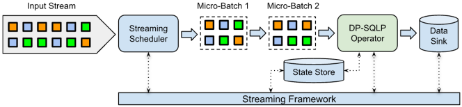
Figure 3: High-level overview for the DP-SQLP system

The streaming differential privacy mechanism described in this paper can be generally applied to various streaming frameworks, including Spark Streaming[48], Apache Beam[3] and Apache Flink[9]. The DP-SQLP system we develop is implemented using a streaming framework similar to Spark Streaming[48], as shown in Figure 3.

The input data stream contains unordered, unbounded event records. The streaming scheduler will first assign each record to the corresponding event-time window $w$. Within each window, at every triggering timestamp $tr$, records are bundled together to create an immutable, partitioned datasets, called a micro-batch. After a micro-batch is created, it will be dispatched to the DP-SQLP operator for processing.

When processing a micro-batch, the DP-SQLP operator will interact with the system state store for a state update. Once the differentially private histogram is generated, it will be materialized to the data sink. Similar to Spark Streaming, our streaming framework provides consistent, ”exactly-once” processing semantic across multiple data centers. In addition, the streaming framework also provides fault tolerance and recovery.

There are multiple ways to schedule micro-batches based on certain rules[3], like processing timer based trigger, data arrival based trigger and combinations of multiple rules.

Based on the number of micro-batches received by operator at each time instance, we can also classify scheduling methods into two categories, sequential scheduling and parallel scheduling, as shown in the Figure 4. In sequential scheduling, input data stream is divided into a sequence of micro-batches. The operator will process one micro-batch at a time. Parallel scheduling is able to further scale up the pipeline, by allowing multiple micro-batches to be processed at the same time. The streaming scheduler will partition records by predefined key tuples, and create one micro-batch per key range.

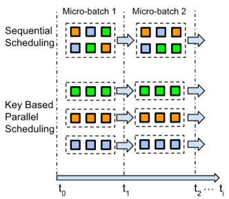
Figure 4: Two types of streaming scheduling

In the rest of paper, we will assume the sequential scheduling for the algorithm discussion. Given data stream $D_{w_{i}}$ for window $w_{i}$, the sub-stream at triggering timestamp $tr_{i}\in\texttt{Tr}_{w_{i}}$ can be denoted as $D_{tr_{i}}\subseteq D_{w_{i}}$, and the sub-stream for each micro-batch can be represented as the incremental data stream $\Delta D_{tr_{i}}=D_{tr_{i}}-D_{tr_{i-1}}$.

As Akidau pointed out in the unified dataflow model [3], batch, micro-batch, and pure streaming are implementation details of the underlying execution engine. Although the streaming differential privacy mechanism discussed in this paper is executed by a streaming system based on micro-batch, the mechanism and algorithm can be widely applied to batch, micro-batch, and pure streaming systems.

It is worth noting that different execution modes (batch, micro-batch and pure streaming) result in different trade-offs between data utility and pipeline latency. In differential privacy, the more frequent we repeat the process, the nosier results tend to be. Therefore, data utility is an additional factor when choosing execution modes.

3 Streaming Private Mechanism

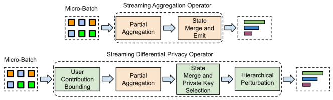
Figure 5: Overview of streaming differential privacy mechanism

In this section we will discuss the overall mechanism for streaming differential privacy. Our target is to perform aggregation and release histogram at every triggering timestamp in Tr, while maintaining $(\varepsilon,\delta)$-differential privacy. There are four main components within streaming differential privacy mechanism – user contribution bounding, partial aggregation, streaming private key selection and hierarchical perturbation.

To simplify the discussion, we will assume Sum is the aggregation function for GROUP BY . It is also possible to use other aggregation function within streaming differential privacy mechanism.

Let’s declare the inputs, parameters and outputs that will be used in streaming differential privacy.

• Input: Data Stream $D$, event-time windows $W$, triggering timestamp per window $\texttt{Tr}_{w}$, privacy parameters $\varepsilon,\delta>0$, accuracy parameter $\beta>0$, per record clamping limit $L$.

• System Parameters: Max. number of records per user $C$.

• Output: Aggregated DP histogram at every triggering timestamp.

3.1 Non-Private Streaming Aggregation

The traditional streaming aggregation operator without differential privacy is shown on the top of Figure 5. Records within the micro-batch are grouped by key and aggregated by the reduce function [48]. After that, the partial aggregation result will be merged with the previous state [44] and the update histogram is emitted. There is no differential privacy protection within this process, and user privacy can be leaked from multiple dimensions, including histogram value, aggregation key and the differences between two histogram updates.

3.2 User Contribution Bounding

DP algorithms require that the sensitivity of each user contributions be limited, for example that a user can contribute up to $C$ times. However, in reality, each user may contribute to many records and many keys, especially for heavy users. Therefore, we need to bound the maximum influence any user can have on the output in order to achieve a desired overall DP guarantee. This step is called “user contribution bounding”.

Some one-shot mechanisms perform user contribution bounding by limiting contributed value per key and the number of contributed keys per user [4, 47]. However, this approach does not fit the streaming setting, since it requires three shuffle stages - shuffle by user, shuffle by (key, user) and shuffle by key.

User contribution bounding in streaming DP is performed on the user level for the entire data stream $D$:

• Each user can contribute to at most $C$ records in the data stream $D$.

• The value $v$ for the aggregation column $m$ in each record is clamped to $L_{m}$ so that $|v|<L_{m}$.

The maximum number of records per user $C$ and per record clamping limit $L_{m}$ together determine the per-user $\ell_{1}$ sensitivity in data stream:

$$L_{1}=C\times L_{m}.$$

Choosing the right contribution bounding parameters $C$ and $L_{m}$ is critical for privacy-utility trade-off. When the bounding limit is small, the noise is small, but the data loss may be significant (e.g. if most/all users have a lot of data to contribute). On the other side, when the bounding limit is large, the data loss is small, but noise is large. It is possible to find a near optimal point from a heuristic study, which we discuss in Section 5. Indeed, one approach to choosing a good a contribution bound is to inspect the data distribution. For example, we can pick $C$ at $99^{th}$ percentile of per-user records (i.e. $<1\%$ users have more than C records), which can be chosen in a DP way if computed on a fraction of the data stream, or in a non-DP way if it is based on proxy data.

In the following sections, we will introduce streaming private key selection and hierarchical perturbation, which are two main private operations in streaming differential privacy. Since the private operations are performed per window, we will focus on $D_{w_{i}}$ during algorithm discussion. However, the same private operations should be applied to all windows.

3.3 Streaming Private Key Selection

The main objective we consider in this section is to select the set of keys that exceed a certain threshold of user contributions $\mu\geq 0$. (These are the keys that are used later for releasing the aggregation columns in Section 3.4 below.) Recall that our streaming system is input driven by a growing data stream, meaning, one only sees the existence of a key if it has at least one user contribution. This poses a significant privacy challenge since the detectable set of keys is highly dependent on the data set. As a result, we design a novel thresholding scheme coupled with binary tree aggregation [17, 11, 24] that allows one to only operate with keys that deterministically have at least $\mu$ user contributions, and still preserve $(\varepsilon,\delta)$-DP. In the following, we provide a description of the algorithm, along with the privacy analysis.

Data preprocessing: After user contribution bounding (discussed in Section 3.2), we first perform a regular key GROUP BY and aggregation for all records within the current micro-batch. Then we aggregate the user data via GROUP BY on each key and merge results with a data buffer that is stored in a system state. Beyond that we execute the key selection algorithm described in Algorithm 2.

Algorithm description: As mentioned earlier, the emitted key space is not predefined. A key may emerge when there is at least one user record with the key (due to the nature of input driven stream). Therefore, the streaming DP system must determine when and what keys to release or update, in a private manner. This is different from the non-private streaming aggregation, where updates will be emitted at every triggering timestamp after processing each micro-batch.

Remark: In the description of Algorithm 2, we use the following primitives implicitly used in Algorithm 1: i) ${\texttt{InitializeTree}}\,(T,\sigma)$: Initialize a complete binary tree $\mathcal{T}$ with $2^{\lceil T\rceil}$ leaf nodes with each node being sampled from $\mathcal{N}(0,\sigma^{2})$, ii) ${\texttt{AddToTree}}\,(\mathcal{T},i,c_{i})$: Add $c_{i}$ to all the nodes on the path from the $i$-th leaf node to the root of the tree, and iii) ${\texttt{GetTotalSum}}\,(\mathcal{T}_{\texttt{key}}\,,i)$: Prefix sum of the all the inputs $\{c_{1},\ldots,c_{i}\}$ to the binary tree computed via Algorithm 1.

Our approach is an extension of thresholding algorithm in [30] to the streaming setting. In short, we carefully select a threshold and compute (with DP noise) the number of data records that contributed to each encountered key. If this noisy number is greater than or equal to the chosen threshold, the key is released. We describe the algorithm in full detail in Algorithm 2, and provide the formal privacy guarantee in Theorem 3.1.

A crucial component of the algorithm is the choice of the threshold $\tau$ in Line 2 of Algorithm 2. One can instantiate $\tau$ with the bound in Theorem 2.4. However, in our implementation (described in Section 4) we actually implement the tree aggregation via the “bottom-up Honaker” variance reduction described in Section 2.2. One can write the exact distribution of the differences between DP-Tree aggregated count and the true count, which is $\hat{q}_{{tr_{i},k}}-\texttt{count}_{k}(D_{tr_{i}})$ in Line 2 of Algorithm 2, via (2). This allows us to get a tighter bound on $\tau$ based on the inverse CDF of the Gaussian distribution. Also, it should be obvious from (2) that the variance of the Gaussian distribution is dependent on the time step at which we are evaluating the cumulative sum. Hence, to obtain a tighter estimation of the threshold, we actually have a time dependent threshold $\tau_{tr_{i}}$ (based on (2)) instead of an universal threshold in Line 2.

Remark: For brevity, in Theorems 3.1 and 3.2, we provide the guarantees assuming each user only contributes once, i.e., in the language of Section 3.2 we assume that that user contribution bound $C=1$. However, in our implementation we do allow $C>1$. The idea is to use a tighter variant of advanced composition for $(\varepsilon,\delta)$-DP [19] while ensuring that each user contributes at most once to each key in any instance of Algorithm 2.

Algorithm 2 Streaming Private Key Selection

0:  Data stream $D_{w_{i}}=\{d_{1},\ldots,d_{n}\}$, where the event timestamp $t_{i}$ of each $d_{i}$ can map to event-time window $w_{i}=(t_{s},t_{e})$, $t_{s}<t_{i}<t_{e}$, triggering timestamps $\texttt{Tr}_{w_{i}}=[tr_{1},tr_{2},...,tr_{T_{i}}]$. At each triggering time $tr_{i}\subseteq\mathbb{R}$, only a sub-stream $D_{tr_{i}}\subseteq D_{w_{i}}$ is available. Threshold $\mu\geq 0$, privacy parameters $\varepsilon,\delta>0$, failure probability $\beta>0$.

1:  Compute the noise standard deviation $\sigma$ for the tree aggregation based on $(T_{i}=|\texttt{Tr}_{w_{i}}|,\varepsilon,\delta)$. (See Appendix B for more details.)

2:  Compute the accuracy threshold $\tau$ of the tree aggregation such that for any fixed key  and the corresponding binary tree $\mathcal{T}_{\texttt{key}}\,$,

$${\underset{\mathcal{T}_{\texttt{key}}\,}{\mathbb{P}}\left[\forall tr_{i}\in\texttt{Tr}_{w},|\hat{q}_{{tr_{i},\texttt{key}\,}}-\texttt{count}_{\texttt{key}}\,(D_{tr_{i}})|\leq\tau\right]}\geq 1-\beta,$$

which depends on $\sigma$ and $\beta$. (See Appendix B for more details.) Here, $\texttt{count}_{\texttt{key}}\,(D_{tr_{i}})$ denote the unique user count for key  in $D_{tr_{i}}$, and $\hat{q}_{{tr_{i},\texttt{key}\,}}$ denote the private estimate of $\texttt{count}_{\texttt{key}}\,(D_{tr_{i}})$.

3:  for $i\in|\texttt{Tr}_{w_{i}}|$ do

4:     $\mathcal{S}^{(i)}\leftarrow$ Set of all keys in the stream $D_{tr_{i}}$ with count $>\mu$.

5:     For all $\texttt{key}\,\in\mathcal{S}^{(i)}\backslash\mathcal{S}^{(i-1)}$, create a new tree $\mathcal{T}_{\texttt{key}\,}$ using ${\texttt{InitializeTree}}\,(T_{i},\sigma)$, and execute Algorithm 1 till $(i-1)$-th step with all zeros as input.

6:     for $\texttt{key}\,\in\mathcal{S}^{(i)}$ do

7:        $\mathcal{T}_{\texttt{key}}\,\leftarrow{\texttt{AddToTree}}\,\left(\mathcal{T}_{\texttt{key}}\,,i,\texttt{count}_{\texttt{key}}\,(D_{tr_{i}})-\texttt{count}_{\texttt{key}}\,(D_{tr_{i-1}})\right)$, i.e., Add the count at time stamp $tr_{i}$ to $\mathcal{T}_{\texttt{key}\,}$.

8:        $\hat{q}_{{tr_{i},\texttt{key}\,}}\leftarrow{\texttt{GetTotalSum}}\,(\mathcal{T}_{\texttt{key}}\,,i)$.

9:        if $\hat{q}_{{tr_{i},\texttt{key}\,}}>\mu+\tau$, then output $(\texttt{key}\,,\hat{q}_{{tr_{i},\texttt{key}\,}})$.

10:     end for

11:  end for

Theorem 3.1 (Privacy guarantee).

Algorithm 2 is $(\varepsilon,\delta+(e^{\varepsilon}+1)\cdot\beta)$-DP for addition or removal of one element of the dataset.

Proof.

Consider two datasets $D$ and $D^{\prime}$ which differ by the addition or removal of one key $k_{*}$. Let $A(D)$ denote Algorithm 2 run on input $D$. First we note that we can ignore all other keys $k\neq k_{*}$ because the behaviour of Algorithm 2 on those keys is independent of its behaviour with respect to $k_{*}$.

For the purposes of the analysis, we consider a different algorithm $A^{\prime}(D)$ which does the following with respect to $k_{*}$. It initializes the tree aggregation mechanism $\mathcal{T}_{k_{*}}$ at the beginning. At each time $t\in\texttt{Tr}$, the algorithm $A^{\prime}(D)$ computes $\hat{q}_{t,k_{*}}\leftarrow{\texttt{GetTotalSum}}\,(\mathcal{T}_{k_{*}})$. If $\hat{q}_{t,k_{*}}>\mu+\tau$, then it outputs $(k_{*},\hat{q}_{t,k_{*}})$; otherwise it outputs nothing about $k_{*}$ at time $t$.

The algorithm $A^{\prime}$ is $(\varepsilon,\delta)$-DP. This is because it is simply a postprocessing of the tree aggregation mechanism, which is set to have this DP guarantee.

The only difference between the outputs of $A(D)$ and $A^{\prime}(D)$ is that, if $\texttt{count}_{k_{*}}(D_{t_{i}})\leq\mu$ and $\hat{q}_{t,k_{*}}>\mu+\tau$, then $A^{\prime}(D)$ outputs $(k_{*},\hat{q}_{t,k_{*}})$, but $A(D)$ outputs nothing regarding $k_{*}$. Since $\hat{q}_{t,k_{*}}>\mu+\tau$ is meant to be an approximation to $\texttt{count}_{k_{*}}(D_{t_{i}})\leq\mu$, this means the outputs only differ when the tree aggregation mechanism $\mathcal{T}_{k_{*}}$ has error $>\tau$. The accuracy guarantee of $\mathcal{T}_{k_{*}}$ ensures this happens with probability at most $\beta$. That is, we can define a coupling such that ${\mathbb{P}\left[A(D)\neq A^{\prime}(D)\right]}\leq\beta$ (and the same for $D^{\prime}$ in place of $D$).

Thus we can obtain the DP guarantee for $A$: Let $E$ be an arbitrary measurable set of outputs of $A$. We have

$${\mathbb{P}\left[A(D)\in E\right]} \leq{\mathbb{P}\left[A^{\prime}(D)\in E\right]}+{\mathbb{P}\left[A(D)\neq A^{\prime}(D)\right]}$$

$$\leq e^{\varepsilon}\cdot{\mathbb{P}\left[A^{\prime}(D^{\prime})\in E\right]}+\delta+{\mathbb{P}\left[A(D)\neq A^{\prime}(D)\right]}$$

$$\leq e^{\varepsilon}\cdot({\mathbb{P}\left[A(D^{\prime})\in E\right]}+{\mathbb{P}\left[A(D)\neq A^{\prime}(D)\right]})+\delta$$

$$\ \ \ \ +{\mathbb{P}\left[A(D)\neq A^{\prime}(D)\right]}$$

$$=e^{\varepsilon}\cdot{\mathbb{P}\left[A(D^{\prime})\in E\right]}+\delta+(e^{\varepsilon}+1)\cdot{\mathbb{P}\left[A(D)\neq A^{\prime}(D)\right]}$$

$$\leq e^{\varepsilon}\cdot{\mathbb{P}\left[A(D^{\prime})\in E\right]}+\delta+(e^{\varepsilon}+1)\cdot\beta.$$

∎

Theorem 3.2 (Utility guarantee).

For any fixed key $k$, there exists a threshold $\tau=\mathcal{O}\left(\frac{\sqrt{\log(T/\beta)\log^{2}(T)\log(1/\delta)}}{\varepsilon}\right)$ such that w.p. at least $1-\beta$, Algorithm 2 outputs $k$ if at any one of the triggering time (in $\texttt{Tr}=[tr_{1},tr_{2},...,tr_{T}]$) the true count is at least $\mu+\tau$ .

Proof.

By using Theorem 2.4, and using the notation in Line 2 the following is immediate, when the noise added to each node of the binary tree in Algorithm 2 is $\mathcal{N}(0,\sigma^{2})$. For any fixed key $k$,

$$\begin{split}{\underset{\mathcal{T}_{k}}{\mathbb{P}}\left[\forall tr_{i}\in\texttt{Tr}~{}~{}|\hat{q}_{{tr_{i},k}}-\texttt{count}_{k}(D_{tr_{i}})|\leq\sqrt{\frac{2\ln(T/\beta)\lceil\lg(T)\rceil\sigma^{2}}{\pi}}\right]}\\ \geq 1-\beta.\end{split}$$ (3)

Setting $\sigma^{2}=\frac{2\lceil\lg(T)\rceil\ln(1.25/\delta)}{\varepsilon^{2}}$, and using the translation of zCDP to $(\varepsilon,\delta)$-DP (based on the privacy statement in Theorem 2.3) completes the proof. ∎

3.4 Hierarchical Perturbation

Algorithm 3 Hierarchical Perturbation with DP-Tree

0:  Data stream: $D_{w_{i}}=\{d_{1},\ldots,d_{n}\}$, where each $d_{i}$ arrive at time $t_{i}$ within event-time window $w_{i}=(t_{s},t_{e})$, $t_{s}<t_{i}<t_{e}$. Triggering timestamps $\texttt{Tr}_{w_{i}}=[tr_{1},tr_{2},...,tr_{T_{i}}]$. At each triggering timestamp $tr_{i}\subseteq\mathbb{R}$, only a sub-stream $D_{t}\in D_{w_{i}}$ is available. Privacy parameters $\varepsilon,\delta>0$, number of DP-Tree  leaf nodes $n$.

1:  Compute the noise standard deviation $\sigma$ for the tree aggregation based on $(n,\varepsilon,\delta)$. (See Appendix B for more details.)

2:  for $i\in|\texttt{Tr}_{w_{i}}|$ do

3:     $\mathcal{S}_{i}\leftarrow$ Set of keys output by the key selection algorithm (Algorithm 2) at $tr_{i}$.

4:     for $\texttt{key}\,\in\mathcal{S}_{i}$ do

5:        Let $D_{tr_{i}}\leftarrow$ data stream available at time stamp $tr_{i}$.

6:        Last Release Time $\texttt{LRT}_{\texttt{key}}\,\leftarrow$ triggering timestamp of the previous statistic release.

7:        $\Delta V_{\texttt{key}}\,\leftarrow$ Aggregated value for key  in the sub-stream $D_{tr_{i}}-D_{\texttt{LRT}_{\texttt{key}}\,}$.

8:        $\mathcal{T}_{\texttt{key}}\,\leftarrow{\texttt{AddToTree}}\,(\mathcal{T}_{\texttt{key}}\,,i,\Delta V_{\texttt{key}}\,)$.

9:        Output ${\texttt{GetTotalSum}}\,(\mathcal{T}_{\texttt{key}}\,,i)$.

10:     end for

11:  end for

Once sufficient records of certain key are accumulated (i.e., following the notation from the previous section there are at least $\mu$ unique user contributions), the objective is to select the key for statistic release. Statistic release corresponds to adding the value from user contributions to a main histogram that estimates the distribution of records across all the keys. Notice that in this histogram, a single user can contribute multiple times to the same key. In this section we discuss how to create this histogram while preserving DP.

The crux of the algorithm is that for all the set of keys detected during the key selection phase via Algorithm 2, we maintain a DP-tree (an instantiation of Algorithm 1) for every key detected. We provide a $\rho$-zCDP guarantee for each of the trees for each of the keys. Since each user can contribute $C$ records in this phase, and in the worst case all these contributions can go to the same node of a single binary tree, we scale up the sensitivity corresponding to any single node in the tree to $L_{1}=C\cdot L$ (analogous to that in Section 3.2), and ensure that each tree still ensures $\rho$-zCDP. We provide the details of the algorithm in Algorithm 3. The privacy guarantee follows immediately from Theorem 2.3, and the translation from $\rho$-zCDP to $(\varepsilon,\delta)$-DP guarantee. In Algorithm 3, we will use a lot of the binary tree aggregation primitives we used in Section 3.3.

4 System Implementation and Optimization

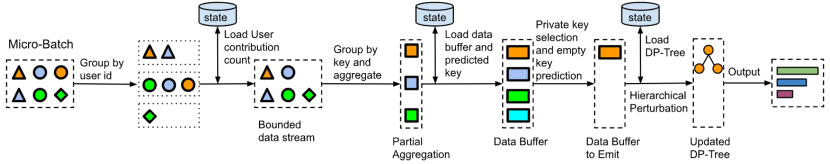
Figure 6: Execution of streaming differential privacy mechanism

When implementing the streaming differential privacy algorithms described in Section 3, one must take the system constraints into practical considerations. There are three main challenges:

• The streaming framework described in Section 2.3 discretizes the data stream into micro-batches. Therefore, streaming key selection and hierarchical perturbation, whose algorithms are defined based on data stream $D_{t^{\texttt{Tr}}_{i}}$, must be implemented using micro-batch $\Delta D_{t^{\texttt{Tr}}_{i}}$ (defined in Section 2.3) and the system state. In Section 4.1 we detail the complete state management of DP-SQLP.

• DP-SQLP is input data stream driven. The state loading and updating require the existence of a key in the current micro-batch. However, Algorithm  2 requires to test all keys that have appeared at least once. In Section 4.3 we discuss a new algorithm that avoids testing all the keys that have appeared at least once.

• There are multiple components to the DP-SQLP system wich are individually $(\varepsilon,\delta)$-DP. It is necessary to use appropriate form of composition to account for the total privacy cost. In Section 4.4, we detail the complete privacy accounnting for DP-SQLP.

4.1 State Management

As mentioned above, both streaming key selection and hierarchical perturbation are defined based on data stream $D_{t^{\texttt{Tr}}_{i}}$. Therefore, they both require stateful operations. Furthermore, the global user contribution bounding that tracks the number of records per-user in data stream $D$ is also stateful.

In DP-SQLP, the system state store is a persistent storage system, backed by Spanner database [13] that provides high availability and fault tolerance. The system state store is co-managed by DP-SQLP operator and the streaming framework for state update and maintenance. All the state information required by streaming differential privacy is stored in the system state store. For a pictorial depiction, see Figure 3.

State Store Structure: There are two main state tables in the system state stores, which are managed by the same streaming framework. Each state table is a key value storage contains  state key and  state object.

The first state table is keyed by user id to track per-user contribution within the data stream. The state object simply stores the count value.

The second state table is keyed by GROUP BY keys. The state object contains data buffer, DP-Trees for key selection and DP-Trees for aggregation columns. Data buffer is a data structure that temporarily stores the unreleased, aggregated data from new records, due to the failure in thresholding test (line 9, Algorithm 2). One DP-Tree is used by each round of Algorithm 2 execution, and one DP-Tree is used for hierarchical perturbation per aggregation column.

Execution Procedures: The execution of streaming differential privacy mechanism is shown in Figure 6. Different shapes represent different users and different colors represent different keys. Each step is described as following.

1. User contribution bounding: Records in one micro-batch are grouped by user id. A map in system state store is maintained to track the number of records each user contributes. Once the number of contributions for a user reaches $C$, all the remaining records for that user in the data stream will be discarded. Furthermore, we clamp the value $v$ of each aggregation column $m$, so that $|v|\leq L_{m}$.

2. Cross-user aggregation: Records in one micro-batch are grouped by key and aggregated, which form a delta result [21]. After that, the delta result will be merged into the data buffer that is loaded from the system state store.

3. Streaming key selection: The DP-Trees for streaming key selection are loaded from the system state store. Then we will perform Algorithm 2, which adds the incremental user count from the current micro-batch into DP-Tree , as a leaf node.

4. Hierarchical perturbation: Once a key is selected, the DP-Tree for hierarchical perturbation is loaded from the system state store. After that, we will use Algorithm 3 to get DP aggregation results, and output the results.

The execution engine used to implement user contribution bounding and hierarchical perturbation will be discussed in section 4.2.

As mentioned in section 3.3, the DP-Tree estimator is implemented with the “bottom-up Honaker” variance reduction to get the DP sum. The estimated sum for DP-Tree root at ${\sf node}_{i^{*}}$ equals

$$\hat{\texttt{Sum}}({\sf node}_{i})=\sum\limits_{j=0}^{\mu-1}c_{j}\cdot{\sf sum}(\texttt{level}_{j}).$$

In case more than one DP-Trees are used in key selection or hierarchical perturbation, we need to further sum the Honaker estimations from each tree together.

4.2 Parallel Execution

Figure 7: Parallel execution within DP-SQLP operator

When building the DP-SQLP operator, we leverage the F1 query engine [39] for its wide range of data sources and distributed query execution (Figure 7). The user contribution bounding step is executed by the user contribution bounding server. The privacy key selection and hierarchical perturbation are executed by the data perturbation server. Both servers contain thousands of workers that are horizontally scalable. Input data is first read by F1 query engine, partitioned, then sent to user contribution bounding server through Remote Procedure Calls (RPCs). After that, the bounded data will stream back to F1, re-partitioned, then being sent to data perturbation server for key selection and hierarchical perturbation.

4.3 Empty Key Release Prediction

Since the data stream is unordered and unbounded, the existence of user contributions within each micro-batch can be arbitrary, as shown in Figure 8. It is possible that some keys do not have any user records in a micro-batch. In the traditional streaming systems, states are not updated unless new records appear in the micro-batch[44]. Therefore, the system only needs to load state with keys from the current micro-batch.

However, the streaming key selection algorithm (Algorithm 2) requires us to perform the thresholding test for the entire key space, and it is possible for a key being selected without new records. An naive approach is to load all the keys with their associated states from the system state store, and run Algorithm 2 directly. Unfortunately, when the key space is large, the I/O cost and memory cost of loading the entire state table is too high. Here, we propose the empty key release prediction algorithm, together with other operational strategy, to solve the scalability challenge.

Figure 8: Some key may not have records within certain micro-batch

Algorithm 4 Empty Key Release Prediction

0:  Data stream: $D_{w}=\{d_{1},\ldots,d_{n}\}$, where each $d_{i}$ arrive at time $t_{i}$ within event-time window $w=(t_{s},t_{e})$, $t_{s}<t_{i}<t_{e}$. Triggering timestamps $\texttt{Tr}_{w}=[tr_{1},tr_{2},...,tr_{T}]$. At each triggering timestamp $tr_{i}\subseteq\mathbb{R}$, only a sub-stream $D_{t}\in D_{w}$ is available. privacy parameters $\varepsilon,\delta>0$. Let j be the current round of key selection.

1:  $\Delta D_{tr_{j}}\leftarrow D_{tr_{j}}-D_{tr_{j-1}}$ (which is the data stream for the micro-batch at $tr_{j}$.

2:  $\mathcal{S}_{tr_{j}}\leftarrow$ All $\texttt{key}\,\in\Delta D_{tr_{j}}$ selected via Algorithm 2 at time $tr_{j}$.

3:  for $\texttt{key}\,\in\mathcal{S}_{tr_{j}}$ do

4:     for $tr_{p}$ from $tr_{j+1}$ to $tr_{|\texttt{Tr}_{w}|}$ do

5:        $D_{tr_{p}}\leftarrow D_{tr_{j}}$, which mimic the data stream at the next triggering timestamp $tr_{p}$, without any new record.

6:        Perform streaming private key selection on $D_{tr_{p}}$ for key  via Algorithm 2 at time $tr_{p}$.

7:        if key  is selected, then write $\left(\texttt{key}\,,tr_{p}\right)$ to state store and break.

8:     end for

9:  end for

Algorithm description for empty key release prediction: There are two scenarios that may trigger a key being selected: key is selected due to additional user contributions, or key is selected due to noise addition without user contributions. The first scenario is naturally handled by streaming system, when processing micro-batch with new records. The secondary scenario is handled by Algorithm 4.

When a micro-batch $\Delta D_{tr_{j}}$ contains key $k$, the streaming private key selection algorithm for key $k$ is applied to the sub-stream $D_{tr_{j}}$. In case $k$ is not selected, we will simulate streaming private key selection algorithm executions from $tr_{j+1}$ to $tr_{|\texttt{Tr}|}$, using sub-stream $D_{tr_{j}}$, and predict if any future release is possible by adding leaf node with zero count. The predicted releasing time is $tr_{p}$, and it is written to the system state store.

After making a release prediction, the DP-SQLP will continue process the next micro-batch. For key $k$ with predicted releasing time $tr_{p}$, there are two cases:

1. $k$ appears in another micro-batch $\Delta D_{tr_{n}}$ before the predicted triggering timestamp ($j<n<p$). In this case, the prior prediction result is discarded. We will perform key selection algorithm for the micro-batch $\Delta D_{tr_{n}}$. All the thresholding test for micro-batches that do not have $k$ between $tr_{j+1}$ and $tr_{n-1}$ have been performed during the prediction phase in the prior micro-batch $D_{tr_{j}}$. In addition, we will make a new prediction for $\Delta D_{tr_{n}}$.

2. $k$ appears in another micro-batch $\Delta D_{tr_{n}}$ after the predicted triggering timestamp ($p<n$). In this case, DP-SQLP have loaded system state for $k$ at the predicted time $tr_{p}$ and release data from the data buffer. We will start a new round of streaming key selection from micro-batch $\Delta D_{tr_{n}}$.

Within these operations, some computations might be wasted (e.g., Case 1). However, when the key space is large, the reductions in I/O cost and memory cost bring in more benefits than the CPU overhead.

The prediction result is stored in the system state. The step to load predicted result is shown in Figure 6. We also add a secondary index on the predicted timestamp to improve the state loading speed.

4.4 Privacy Accounting for DP-SQLP

In DP-SQLP, the privacy costs occur in streaming key selection (Algorithm 2) and hierarchical perturbation (Algorithm 3). Because each user is allowed to contribute at most $C$ records, we use the combination of composition and sensitivity in privacy accounting.

• Privacy accounting for streaming key selection: When executing Algorithm 2 in DP-SQLP, the value added to each leaf node is the unique user count. Therefore, the per-user sensitivity for each DP-Tree is one. In addition, we restart the Algorithm 2 once a key is selected, and data accumulated in data buffer is released immediately. As the result, each user may participate in at most $C$ rounds of key selection. Given the $(\varepsilon,\delta)$ privacy budget for each round of Algorithm 2, the total privacy cost for streaming key selection is calculated using the empirically tighter variant of advanced composition [19] with $C$-fold.

• Privacy accounting for hierarchical perturbation: For each user, in the worst case, all $C$ contributions can go to the same node of a single DP-Tree , we scale up the sensitivity corresponding to any single node in the tree to $L_{1}=C\cdot L$, and ensure that each tree still ensures $\rho$-zCDP. After that, we use the conversaion from [35, Proposition 3] to translate privacy cost from $\rho$-zCDP to $(\varepsilon,\delta)$-DP guarantee .

Finally, the privacy costs of key selection and hierarchical perturbation are combined via advanced composition.

5 Experiments

The experiments are performed using both synthetic and real-world data to demonstrate the data utility and scalability. The streaming DP mechanism is implemented in DP-SQLP operator, as described in section 4.

Baselines: We compare DP-SQLP with two baseline approaches for data utility.

• Baseline 1 - Repeated differential privacy query. Most of the existing DP mechanisms does not have capacity to track user contributions across multiple queries. Therefore, when handling data streams, one common workaround is to repeatedly apply the one-shot DP query to the growing data set in order to get the histogram update. Thus, the overall privacy budget usage is the composition of all queries.

• Baseline 2 - Incremental differential privacy processing. The one-shot differential privacy algorithm is applied separately to each micro-batch, and we can get the final result by aggregating the outputs from each micro-batch. Compared with baseline 1, baseline 2 requires a similar global user contribution bounding system as DP-SQLP.

For both baseline 1 and baseline 2, the one-shot differential privacy mechanism is executed by Plume [4] with the Gaussian mechanism. Each one-shot differential privacy execution guarantees $(\varepsilon,\delta)$-differential privacy. We also adopt the optimal composition theorem for DP [28] to maximize the baseline performance.

Metrics: The data utility is evaluated based on 4 metrics calculated between the ground truth histogram and the differentially private histogram.

• Number of retained keys, which reflects how many keys are discovered during key selection process. It is also known as the $\ell_{0}$ norm.

• $\ell_{\infty}$ norm, which reflects the worst case error

  $$\ell_{\infty}=\max\limits_{k\in\texttt{key space}}(|\hat{M}_{k}-M_{k}|).$$

• $\ell_{1}$ norm, which is an aggregated error

  $$\ell_{1}=\sum\limits_{k\in\texttt{ key space}}(|\hat{M}_{k}-M_{k}|).$$

• $\ell_{2}$ norm, also known as the euclidean norm

  $$\ell_{2}=\sqrt{\sum\limits_{k\in\texttt{key space}}(|\hat{M}_{k}-M_{k}|^{2})}.$$

We choose $\varepsilon=6$ and $\delta=10^{-9}$ as the overall privacy budget for all experiments. Within DP-SQLP, the privacy budget used by the aggregation column is $\varepsilon_{m}=\varepsilon/2$, $\delta_{m}=\delta/3$, and the ones used by key selection is $\varepsilon_{k}=\varepsilon/2$, $\delta_{k}=\delta\times 2/3$. The parameter C is chosen based on the dataset property. In this experiment, we sampled $10\%$ of one day’s data and set $C$ according to the $99$ percentile of per user number of records. There are more discussions on choosing $C$ in Section 5.4.

For both synthetic data and real-world data, We assume the dataset represents data stream within one day. We also shuffle users’ records so that they are randomly distributed within the day. In experiments, the event-time window is also fixed to one day.

In addition to data utility, we also report the performance latency under various micro-batch sizes and number of workers.

5.1 Synthetic Data

The synthetic data is generated to capture the long-tailed nature of real data. There are 10 millions unique users in the synthetic dataset. Each user draws a number of contributed records from a distribution with range $[1,10^{5}]$ and mean 10 according to a Zipf-Mandelbrot distribution. The parameters are chosen so that roughly $15\%$ users contribute to more than 10 records. The key in each record is also sampled from a set of size $10^{6}$, following a Zipf-Mandelbrot distribution. This implies that roughly $1/3$ of records have the first $10^{3}$ keys.

The histogram query task we perform is a simple count query.

⬇

SELECT key, COUNT(*)

FROM SyntheticDataset

GROUP BY key

Listing 2: Histogram query for synthetic data

The per-record clamping limit $L=1$ since the aggregation function is COUNT. We set $C=32$.

All measurements are averaged across 3 runs. The experiments are performed with 100 micro-batches and 1000 micro-batches. Within one day, 100 micro-batches correspond to roughly 15 minute triggering interval, and 1000 micro-batches correspond to roughly 1.5 min triggering interval.

Table 1: Data utility measure with synthetic data $(\varepsilon=6,\delta=10^{-9})$

Metrics	100 Micro-batches
	DP-SQLP	Baseline 1	Baseline 2
Keys	28,338	435	191
$\ell_{\infty}$ Norm	1,391	18,077	21,913
$\ell_{1}$ Norm	17,741,225	50,835,203	58,551,587
$\ell_{2}$ Norm	50,039	430,547	576,425

Metrics	1000 Micro-batches
	DP-SQLP	Baseline 1	Baseline 2
Keys	22,280	0	0
$\ell_{\infty}$ Norm	1,563	25,497	25,497
$\ell_{1}$ Norm	19,395,721	59,052,062	59,052,062
$\ell_{2}$ Norm	58,237	594,382	594,382

The results are shown in Table 1. There are significant data utility improvement comparing DP-SQLP with two baselines. With 100 micro-batches, the number of retained keys is increased by 65 times; the worst case error is reduced by 92%; the $\ell_{1}$ norm is reduced by 65.1% and the $\ell_{2}$ norm is reduced by 88.4%. The utility improvement is even more significant with 1000 micro-batches. The number of retained keys is increased from 0 to 22,280; the worst case error is reduced by 93.9%; the $\ell_{1}$ norm is reduced by 67.2% and the $\ell_{2}$ norm is reduced by 90.2%.

Another observation we have for DP-SQLP is its stability when the number of micro-batches increases. The utility of one-shot differential privacy mechanisms in baseline 1 and baseline 2 degrade quickly, due to the privacy budget split (baseline 1) and data stream split (baseline 2). This degradation sometimes is not linear. The number of retained keys in baseline 1 and 2 is reduced to 0 when the number of micro-batches grows from 100 to 1000. On the contrary, the utility degradation for DP-SQLP is not as significant. Indeed, when the number of micro-batches increases from 100 to 1000, for DP-SQLP, the number of retained keys is reduced by 21%, the worst case error is increased by 12%, the $\ell_{1}$ norm is increased by 9%, and the $\ell_{2}$ norm is increased by 16%.

In summary, DP-SQLP shows a significant utility improvement over one-shot differential privacy mechanisms when continuously generating DP histograms.

5.2 Reddit Data

⬇

SELECT subreddit, COUNT(*)

FROM RedditData

GROUP BY subreddit

Listing 3: Histogram query for the Reddit data

In the next step, we apply the same experiment to real-world data. Webis-tldr-17-corpus [42] is a popular dataset consisting of 3.8 million posts associated with 1.4 million users on the discussion website Reddit. Our task is to count the user participation per subreddit (specific interest group on Reddit).

We set $C=17$ and the rest experiment settings are the same as the synthetic data. All measurements are averaged across 3 runs.

Table 2: Data utility measure with the Reddit data $(\varepsilon=6,\delta=10^{-9})$

Metrics	100 Micro-batches
	DP-SQLP	Baseline 1	Baseline 2
Keys	1,473	32	63
$\ell_{\infty}$ Norm	102,250	267,147	103,546
$\ell_{1}$ Norm	989,249	2,721,349	2,376,937
$\ell_{2}$ Norm	127,721	322,739	156,472

Metrics	1000 Micro-batches
	DP-SQLP	Baseline 1	Baseline 2
Keys	1,181	9	3
$\ell_{\infty}$ Norm	102,218	266,391	108,124
$\ell_{1}$ Norm	1,074,724	3,081,542	3,074,655
$\ell_{2}$ Norm	127,830	341,557	242,482

The results are summarized in Table 2, and we have similar observations as in the synthetic data experiments. DP-SQLP demonstrates significant utility improvements in the number of retained keys, $\ell_{1}$ norm and $\ell_{2}$ norm, as well as the performance stability when the number of micro-batches grows from 100 to 1000.

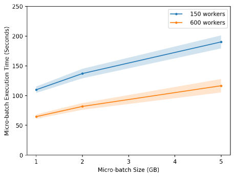
Figure 9: Micro-batch execution time $(\varepsilon=6,\delta=10^{-9})$

5.3 Execution Performance

The end-to-end latency of a record consists of framework latency and micro-batch execution latency. The former is determined by the streaming framework. The latter is a critical indicator for the system scalability. In this section, we report the execution latency for each micro-batch, under different micro-batch sizes and number of workers.

The results are shown in Figure 9. All measurements are averaged across 2 runs, with shaded regions representing standard error. The execution latency grows sub-linearly as the micro-batch size increases. For example, with 150 workers, the execution latency grows 1.7 times while the data size increases 5 times from 1 GB to 5 GB.

Figure 9 also demonstrates horizontal scalability by trading machine resources with latency. When the total number of workers increases from 150 to 600, the execution latency is reduced by 41%, 40%, and 39% respectively for 1, 2, and 5 GB micro-batches.

To further test the scalability in terms of the size of key space, we generate another large synthetic dataset with 1 billion users. Each user draws the number of contributed records following Zipf-Mandelbrot distribution, generating 6 billion records in total. The key in each record is sampled from 1 billion keys following uniform distribution. When setting the micro-batch size equals 1GB and using 5500 workers, the average execution latency is 306 seconds. DP-SQLP easily handle the large load without incurring any significant performance hit.

5.4 Parameter Tuning

Tuning user contribution bounding is critical to achieve good data utility. If $C$ is too small, lots of user records may be dropped due to user contribution bounding, which will lead to large histogram error. However, if $C$ is very large, the noise and key selection threshold are scaled up accordingly. Choosing the right $C$ is an optimization task.

In this section, we run the DP-SQLP with synthetic data using variable $C$ from $1$ to $50$. Figure 10 shows how the change of $C$ affects the number of retained keys, $\ell_{1}$ norm, $\ell_{2}$ norm and $\ell_{\infty}$ norm. The optimal value for $C$ (naturally) varies under different metrics. For example, the optimal $C$ for $\ell_{1}$ norm is around 25 whereas the optimal $C$ for $\ell_{2}$ norm is around 30. In comparison, the optimal $C$ for the number of retained key is around 5. Therefore, the optimal value of $C$ should be chosen according to the metric we care most about (e.g., $\ell_{2}$ norm). In real applications, we could use the $P99$ percentile value or DP $P99$ percentile value from data sample as the starting point and perform few rounds of tests to search for the optimal point.

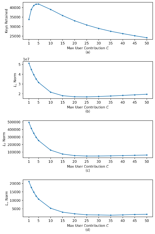
Figure 10: Metrics under different contribution limit $(\varepsilon=6,\delta=10^{-9})$

6 Conclusion and Future Work

In this paper, we presented a streaming differentially private system (DP-SQLP) that is designed to continuously release DP histograms using existing distributed stream processing systems. With user contribution bounding, streaming key selection, and hierarchical perturbation, we provide a formal $(\varepsilon,\delta)$-user level DP guarantee for arbitrary data streams. In addition to the algorithmic design, we implemented our system using a streaming framework similar to Spark streaming, Spanner database, and F1 query engine from Google. The experiments were conducted using both synthetic data and Reddit data. We compared DP-SQLP with two baselines that use one-shot differential privacy algorithms (and privacy accumulation was composed over time). The experiment results demonstrated a significant performance improvement in terms of data utility.

There are three main ways in which our system can be further extended. First, due to the nature of the underlying streaming system (i.e., an input driven stream), we cannot protect the event times of a user. It would be interesting to redesign stream processing systems that compatible with DP even in the context of protecting the event timestamps. Second, our algorithms are primarily designed to provide a centralized DP guarantee, where the final outcome of the system is guaranteed to be DP. It is worth exploring DP streaming system designs that allow stronger privacy guarantees like pan-privacy [18]. Third, we bound the contribution of each user globally by $C$. However, for higher fidelity, it is important to explore approaches to perform per-key contribution bounding. Naive approaches that can address this issue can get complicated due to the fact that we are dealing with an input driven stream.

Appendix A Terms from Streaming Data Processing

Definition A.1 (Input driven stream processing).

For a stream processing system, the statistic release is driven by inputs. The output computation is based on the current input (stateless), or a sequence of inputs (stateful) [44].

Definition A.2 (Event time and event time domain).

Event time is the time at which the event itself actually occurred, i.e. a record of system clock time (for whatever system generated the event) at the time of occurrence. Each event timestamp is determined from a discrete, ordered domain, which is called event time domain [41].

Definition A.3 (Processing time and processing time domain).

Processing time is the time at which an event is observed by the stream processing system, i.e. the current time according to the system clock. Each processing timestamp is determined from a discrete, ordered domain, which is called processing time domain.

Definition A.4 (Windowing).

Windowing slices up a dataset into finite chunks for processing as a group. It determines where in event time data are grouped together for processing [3]. Some common windows include fixed windows, sliding windows and sessions.

Definition A.5 (Triggering).

Trigger is a mechanism to stimulate the output of a specific window at a grouping operation. It determines when in processing time the results of groupings are emitted as panes [3]. There are many ways to define a trigger, including watermark, processing time timers and data arrival.

Definition A.6 (Micro-batch).

Each micro-batch is a partitioned dataset. The continuous data stream is discretized into many micro-batches [3], and the execution of each micro-batch resembles continuous processing.

Appendix B Missing Details from Algorithm 2

In this section, we provide the missing details for the key selection algorithm (Algorithm 2).

Setting $\sigma$ in Line 1: The binary tree has at most $T=|\texttt{Tr}|$ nodes. By Theorem 2.3, the tree aggregation algorithm satisfies $\rho=\frac{\lceil\log_{2}(T)\rceil}{2\sigma^{2}}$-zCDP. Now, we translate the zCDP guarantee into $(\varepsilon,\delta)$-DP (with $\varepsilon$ being a parameter of $\sigma$) via [35, Proposition 2.3] . Using this we obtain $\sigma$ as a function of fixed $\varepsilon$ and $\delta$ and $T$, when used as parameter in Algorithm 2 is guaranteed to ensure $(\varepsilon,\delta)$-DP for the binary tree used there.

Computing accuracy threshold in Line 2: Consider the tree $\mathcal{T}_{k}$, and nodes $\texttt{node}_{1},\ldots,\texttt{node}_{k}$ (from the tree $\mathcal{T}_{k}$) required in the computation of $\hat{q}_{{tr_{i},k}}$ By (2), we have the following:

$$\hat{q}_{{tr_{i},k}}-\texttt{count}_{k}(D_{tr_{i}})\sim\mathcal{N}\left(0,\underbrace{\sum\limits_{j=1}^{k}{\sf Variance}({\sf node}_{j})}_{\lambda^{2}}\right).$$ (4)

In (4), ${\sf Variance}({\sf node}_{j})$ is obtained by (1). We now compute $\tau$ based on the inverse cdf of $\mathcal{N}(0,\lambda^{2})$ at $1-\beta$.

References

- [1]
- Agarwal and Singh [2017] Naman Agarwal and Karan Singh. 2017. The price of differential privacy for online learning. In International Conference on Machine Learning. PMLR, 32–40.
- Akidau et al. [2015] Tyler Akidau, Robert Bradshaw, Craig Chambers, Slava Chernyak, Rafael J Fernández-Moctezuma, Reuven Lax, Sam McVeety, Daniel Mills, Frances Perry, Eric Schmidt, et al. 2015. The dataflow model: a practical approach to balancing correctness, latency, and cost in massive-scale, unbounded, out-of-order data processing. (2015).
- Amin et al. [2022] Kareem Amin, Jennifer Gillenwater, Matthew Joseph, Alex Kulesza, and Sergei Vassilvitskii. 2022. Plume: Differential Privacy at Scale. arXiv preprint arXiv:2201.11603 (2022).
- Amin et al. [2019] Kareem Amin, Alex Kulesza, Andres Munoz, and Sergei Vassilvtiskii. 2019. Bounding user contributions: A bias-variance trade-off in differential privacy. In International Conference on Machine Learning. PMLR, 263–271.
- Andrés et al. [2013] Miguel E Andrés, Nicolás E Bordenabe, Konstantinos Chatzikokolakis, and Catuscia Palamidessi. 2013. Geo-indistinguishability: Differential privacy for location-based systems. In Proceedings of the 2013 ACM SIGSAC conference on Computer & communications security. 901–914.
- Bun and Steinke [2016] Mark Bun and Thomas Steinke. 2016. Concentrated differential privacy: Simplifications, extensions, and lower bounds. In Theory of Cryptography Conference. Springer, 635–658.
- Calandrino et al. [2011] Joseph A. Calandrino, Ann Kilzer, Arvind Narayanan, Edward W. Felten, and Vitaly Shmatikov. 2011. “You Might Also Like:” Privacy Risks of Collaborative Filtering. In 32nd IEEE Symp. on Security and Privacy. 231–246.
- Carbone et al. [2015] Paris Carbone, Asterios Katsifodimos, Stephan Ewen, Volker Markl, Seif Haridi, and Kostas Tzoumas. 2015. Apache Flink™: Stream and Batch Processing in a Single Engine. IEEE Data Eng. Bull. 38, 4 (2015), 28–38. http://sites.computer.org/debull/A15dec/p28.pdf
- Cardoso and Rogers [2022] Adrian Rivera Cardoso and Ryan Rogers. 2022. Differentially private histograms under continual observation: Streaming selection into the unknown. In International Conference on Artificial Intelligence and Statistics. PMLR, 2397–2419.
- Chan et al. [2011] T.-H. Hubert Chan, Elaine Shi, and Dawn Song. 2011. Private and Continual Release of Statistics. ACM Trans. on Information Systems Security 14, 3 (Nov. 2011), 26:1–26:24.
- Cho et al. [2020] Hyunghoon Cho, Daphne Ippolito, and Yun William Yu. 2020. Contact tracing mobile apps for COVID-19: Privacy considerations and related trade-offs. arXiv preprint arXiv:2003.11511 (2020).
- Corbett et al. [2013] James C Corbett, Jeffrey Dean, Michael Epstein, Andrew Fikes, Christopher Frost, Jeffrey John Furman, Sanjay Ghemawat, Andrey Gubarev, Christopher Heiser, Peter Hochschild, et al. 2013. Spanner: Google’s globally distributed database. ACM Transactions on Computer Systems (TOCS) 31, 3 (2013), 1–22.
- Denisov et al. [2022] Sergey Denisov, Brendan McMahan, Keith Rush, Adam Smith, and Abhradeep Thakurta. 2022. Improved differential privacy for sgd via optimal private linear operators on adaptive streams. arXiv preprint arXiv:2202.08312 (2022).
- Dwork et al. [2006a] Cynthia Dwork, Krishnaram Kenthapadi, Frank McSherry, Ilya Mironov, and Moni Naor. 2006a. Our data, ourselves: Privacy via distributed noise generation. In Advances in Cryptology—EUROCRYPT. 486–503.
- Dwork et al. [2006b] Cynthia Dwork, Frank McSherry, Kobbi Nissim, and Adam Smith. 2006b. Calibrating Noise to Sensitivity in Private Data Analysis. In Proc. of the Third Conf. on Theory of Cryptography (TCC). 265–284. http://dx.doi.org/10.1007/11681878_14
- Dwork et al. [2010a] Cynthia Dwork, Moni Naor, Toniann Pitassi, and Guy N. Rothblum. 2010a. Differential Privacy Under Continual Observation. In Proc. of the Forty-Second ACM Symp. on Theory of Computing (STOC’10). 715–724.
- Dwork et al. [2010b] Cynthia Dwork, Moni Naor, Toniann Pitassi, Guy N Rothblum, and Sergey Yekhanin. 2010b. Pan-Private Streaming Algorithms.. In ics. 66–80.
- Dwork and Roth [2014] Cynthia Dwork and Aaron Roth. 2014. The algorithmic foundations of differential privacy. Foundations and Trends in Theoretical Computer Science 9, 3–4 (2014), 211–407.
- Dwork and Rothblum [2016] Cynthia Dwork and Guy N Rothblum. 2016. Concentrated differential privacy. arXiv preprint arXiv:1603.01887 (2016).
- Fegaras [2016] Leonidas Fegaras. 2016. Incremental query processing on big data streams. IEEE Transactions on Knowledge and Data Engineering 28, 11 (2016), 2998–3012.
- Fragkoulis et al. [2020] Marios Fragkoulis, Paris Carbone, Vasiliki Kalavri, and Asterios Katsifodimos. 2020. A survey on the evolution of stream processing systems. arXiv preprint arXiv:2008.00842 (2020).
- Henzinger and Upadhyay [2022] Monika Henzinger and Jalaj Upadhyay. 2022. Constant matters: Fine-grained Complexity of Differentially Private Continual Observation Using Completely Bounded Norms. arXiv preprint arXiv:2202.11205 (2022).
- Honaker [2015] James Honaker. 2015. Efficient use of differentially private binary trees. Theory and Practice of Differential Privacy (TPDP 2015), London, UK (2015).
- Isah et al. [2019] Haruna Isah, Tariq Abughofa, Sazia Mahfuz, Dharmitha Ajerla, Farhana Zulkernine, and Shahzad Khan. 2019. A survey of distributed data stream processing frameworks. IEEE Access 7 (2019), 154300–154316.
- Jain et al. [2012] Prateek Jain, Pravesh Kothari, and Abhradeep Thakurta. 2012. Differentially Private Online Learning. In Proc. of the 25th Annual Conf. on Learning Theory (COLT), Vol. 23. 24.1–24.34.
- Kairouz et al. [2021] Peter Kairouz, Brendan McMahan, Shuang Song, Om Thakkar, Abhradeep Thakurta, and Zheng Xu. 2021. Practical and private (deep) learning without sampling or shuffling. In International Conference on Machine Learning. PMLR, 5213–5225.
- Kairouz et al. [2017] Peter Kairouz, Sewoong Oh, and Pramod Viswanath. 2017. The Composition Theorem for Differential Privacy. IEEE Trans. Inf. Theory 63, 6 (2017), 4037–4049. https://doi.org/10.1109/TIT.2017.2685505
- Kamath et al. [2023] Gautam Kamath, Argyris Mouzakis, Matthew Regehr, Vikrant Singhal, Thomas Steinke, and Jonathan Ullman. 2023. A Bias-Variance-Privacy Trilemma for Statistical Estimation. arXiv preprint arXiv:2301.13334 (2023).
- Korolova et al. [2009] Aleksandra Korolova, Krishnaram Kenthapadi, Nina Mishra, and Alexandros Ntoulas. 2009. Releasing search queries and clicks privately. In Proceedings of the 18th international conference on World wide web. 171–180.
- Latif et al. [2020] Sufian Latif, Yu Hao, Hailong Zhang, Raef Bassily, and Atanas Rountev. 2020. Introducing differential privacy mechanisms for mobile app analytics of dynamic content. In 2020 IEEE International Conference on Software Maintenance and Evolution (ICSME). IEEE, 267–277.
- Li et al. [2015] Chao Li, Gerome Miklau, Michael Hay, Andrew McGregor, and Vibhor Rastogi. 2015. The matrix mechanism: optimizing linear counting queries under differential privacy. The VLDB journal 24, 6 (2015), 757–781.
- Liu et al. [2018] Jianqing Liu, Chi Zhang, and Yuguang Fang. 2018. Epic: A differential privacy framework to defend smart homes against internet traffic analysis. IEEE Internet of Things Journal 5, 2 (2018), 1206–1217.
- Liu et al. [2022] Yuhan Liu, Ananda Theertha Suresh, Wennan Zhu, Peter Kairouz, and Marco Gruteser. 2022. Histogram Estimation under User-level Privacy with Heterogeneous Data. arXiv preprint arXiv:2206.03008 (2022).
- Mironov [2017] Ilya Mironov. 2017. Rényi differential privacy. In 2017 IEEE 30th Computer Security Foundations Symposium (CSF). IEEE, 263–275.
- Papernot et al. [2020] Nicolas Papernot, Steve Chien, Shuang Song, Abhradeep Thakurta, and Ulfar Erlingsson. 2020. Making the Shoe Fit: Architectures, Initializations, and Tuning for Learning with Privacy. https://openreview.net/forum?id=rJg851rYwH
- Perrier et al. [2018] Victor Perrier, Hassan Jameel Asghar, and Dali Kaafar. 2018. Private continual release of real-valued data streams. arXiv preprint arXiv:1811.03197 (2018).
- Phelan et al. [2009] Owen Phelan, Kevin McCarthy, and Barry Smyth. 2009. Using twitter to recommend real-time topical news. In Proceedings of the third ACM conference on Recommender systems. 385–388.
- Samwel et al. [2018] Bart Samwel, John Cieslewicz, Ben Handy, Jason Govig, Petros Venetis, Chanjun Yang, Keith Peters, Jeff Shute, Daniel Tenedorio, Himani Apte, et al. 2018. F1 query: Declarative querying at scale. Proceedings of the VLDB Endowment 11, 12 (2018), 1835–1848.
- Smith and Thakurta [2013] Adam Smith and Abhradeep Thakurta. 2013. (Nearly) optimal algorithms for private online learning in full-information and bandit settings. In Advances in Neural Information Processing Systems. 2733–2741.
- Srivastava and Widom [2004] Utkarsh Srivastava and Jennifer Widom. 2004. Flexible time management in data stream systems. In Proceedings of the twenty-third ACM SIGMOD-SIGACT-SIGART symposium on Principles of database systems. 263–274.
- Syed et al. [2017] Shahbaz Syed, Michael Voelske, Martin Potthast, and Benno Stein. 2017. Webis-tldr-17 corpus. Zenodo, November (2017).
- Tan et al. [2021] Liang Tan, Keping Yu, Ali Kashif Bashir, Xiaofan Cheng, Fangpeng Ming, Liang Zhao, and Xiaokang Zhou. 2021. Toward real-time and efficient cardiovascular monitoring for COVID-19 patients by 5G-enabled wearable medical devices: a deep learning approach. Neural Computing and Applications (2021), 1–14.
- To et al. [2018] Quoc-Cuong To, Juan Soto, and Volker Markl. 2018. A survey of state management in big data processing systems. The VLDB Journal 27, 6 (2018), 847–872.
- Vadhan [2017] Salil Vadhan. 2017. The complexity of differential privacy. Tutorials on the Foundations of Cryptography: Dedicated to Oded Goldreich (2017), 347–450.
- Wang et al. [2016] Leye Wang, Daqing Zhang, Dingqi Yang, Brian Y Lim, and Xiaojuan Ma. 2016. Differential location privacy for sparse mobile crowdsensing. In 2016 IEEE 16th International Conference on Data Mining (ICDM). IEEE, 1257–1262.
- Wilson et al. [2019] Royce J Wilson, Celia Yuxin Zhang, William Lam, Damien Desfontaines, Daniel Simmons-Marengo, and Bryant Gipson. 2019. Differentially private SQL with bounded user contribution. arXiv preprint arXiv:1909.01917 (2019).
- Zaharia et al. [2013] Matei Zaharia, Tathagata Das, Haoyuan Li, Timothy Hunter, Scott Shenker, and Ion Stoica. 2013. Discretized Streams: Fault-Tolerant Streaming Computation at Scale. In Proceedings of the Twenty-Fourth ACM Symposium on Operating Systems Principles (Farminton, Pennsylvania) (SOSP ’13). Association for Computing Machinery, New York, NY, USA, 423–438. https://doi.org/10.1145/2517349.2522737
- Úlfar Erlingsson et al. [2019] Úlfar Erlingsson, Ilya Mironov, Ananth Raghunathan, and Shuang Song. 2019. That which we call private. arXiv:1908.03566 [cs.LG]