A data-driven method for parametric PDE Eigenvalue Problems using Gaussian Process with different covariance functions

Abstract

We propose a non-intrusive, reduced-basis, and data-driven method for approximating both eigenvalues and eigenvectors in parametric eigenvalue problems. We generate the basis of the reduced space by applying the proper orthogonal decomposition (POD) approach on a collection of pre-computed, full-order snapshots at a chosen set of parameters. Then, we use Bayesian linear regression (a.k.a. Gaussian Process Regression) in the online phase to predict both eigenvalues and eigenvectors at new parameters. A split of the data generated in the offline phase into training and test data sets is utilized in the numerical experiments following standard practices in the field of supervised machine learning. Furthermore, we discuss the connection between Gaussian Process Regression and spline methods, and compare the performance of GPR method against linear and cubic spline methods. We show that GPR outperforms other methods for functions with a certain regularity. To this end, we discuss various different covariance functions which influence the performance of GPR. The proposed method is shown to be accurate and efficient for the approximation of multiple 1D and 2D affine and non-affine parameter-dependent eigenvalue problems that exhibit crossing of eigenvalues.

1 Introduction

PDE eigenvalue problems are an important class of problems in science and engineering. Many eigenvalue problems (EVPs) are dependent on some parameters where the parameters may come from the material properties, geometric domain, or initial or boundary conditions. Parametric eigenvalue problems are distinguished by the existence of multiple eigenvectors and eigenvalues, allowing for the possibility of intersection. Furthermore, one has to solve such eigenvalue problems for several parameters, such as in many query problems. In such cases, one needs to discretize the domain and assemble the corresponding matrices, making solving such problems very expansive.

In this context, reduced-order modeling comes into the picture. Model order reduction (MOR) techniques allow for fast but accurate computations. In particular, one first generates a collection of snapshots of eigensolutions evaluated at a chosen set of parameters. Such snapshots are generated in two different ways: using a) adaptive greedy algorithms ¹ and b) the proper orthogonal decomposition (POD). This is known as the offline phase. Then, a surrogate is constructed, which is used to approximate the eigensolution at any intermediate parameter. This is the online phase. A popular method is the reduced basis (RB) method which has been developed to approximate one ²⁰ or more ^{26, 22, 21, 17} eigenvalues. Stochastic Galerkin ¹⁵ and stochastic Collocation ² have also been proposed for stochastic EVPs. However, in comparison to progress made in source problems (see for example ^{23, 24}), eigenvalue problems (for more see  ^{6, 12}) are much less studied despite their importance.

Furthermore, a greedy RB method has also been developed to deal with affine and non-affine parametric eigenvalue problems ¹¹, focusing only on a single eigenpair. However, a data-driven approach ³ that uses Gaussian Process Regression (GPR) has also been proposed to deal with both affine and non-affine problems, an approach inspired by a previous work focused on source problems ¹⁴.

In the context of reduced-order models, GPR is used as a surrogate for the parameter-to-eigensolution map in the online phase. In this paper, we explore further applying the Gaussian Process Regression (GPR) in eigenvalue problems. GPR is a statistical approach that is normally used in fields such supervised machine learning. However, its connection to spline methods, which are commonly used in PDE problems, has been known for close to fifty years. Nevertheless, such a connection has not been taken advantage of in solving eigenvalue problems and source problems until very recently.

We introduce GPR and discuss its connection to spline methods in Sections 3 and 4. We also make comparisons in cases where uniform and non-uniform grids are used. We emphasize how the statistical nature of GPR can be utilized to allow for better performance in both cases. Indeed, GPR is representative of statistical approaches used in fields such as machine learning. Spline methods, on the other hand, are the most popular choice for PDE problems. Bridging the gap then will allow for utilizing applied or theoretical techniques developed for PDE problems in machine learning and vice versa.

In addition, we investigate in Section 5 issues related to applying GPR to both affine and non-affine problems. As will be shown, the performance of GPR is heavily influenced by the choice of the covariance function. We thus focus on analyzing the behavior of the solutions for multiple different covariance functions. In particular, as intersections between eigenvalues are possible, the solutions to be approximated might not be smooth. Consequently, we thoroughly discuss the connection between the regularity of the covariance function and the eigensolutions.

2 Parametric eigenvalue problems

Let $\mathcal{M}\subset\mathbb{R}^{d}$ be closed and bounded. In this paper we consider only the case $d\leq 2$. For each $\bm{\mu}\in\mathcal{M}$, we define two symmetric and bilinear forms

$$a(\cdot,\cdot;\bm{\mu}):V\times V\to\mathbb{R},$$

$$b(\cdot,\cdot;\bm{\mu}):H\times H\to\mathbb{R}.$$

where we assume the existence of the following Hilbert triplet $V\subset H\simeq H^{\prime}\subset V^{\prime}$.

We seek to solve the following problem: for all $\bm{\mu}\in\mathcal{M}$, find real eigenvalues $\lambda(\bm{\mu})$ and non-vanishing eigenfunctions $u(\bm{\mu})\in V$ such that

$$a(u,v;\bm{\mu})=\lambda(\bm{\mu})b(u,v;\bm{\mu})\quad\forall v\in V.$$ (1)

To ensure that all eigenvalues have finite-dimensional eigenspaces, we make the following assumptions so that we have only a compact solution operator. First, we require that V is compact in H. Second, for all $\bm{\mu}\in\mathcal{M}$, the bilinear form $a(\cdot,\cdot;\bm{\mu})$ must be elliptic in $V$, while $b(\cdot,\cdot;\bm{\mu})$ must be equivalent to the inner product in $H$.

For each $\bm{\mu}\in\mathcal{M}$, we only solve for $m_{s}$ high-fidelity eigensolutions, namely the eigenvalue and the associated eigenvector. We do this by discretizing using finite elements. In other words, we consider a finite-dimensional subspace $V_{h}\subset V$ of dimension $n_{h}$. Then, for all $\bm{\mu}\in\mathcal{M}$, we consider the eigensolutions for the following generalized eigenvalue problem: find the real eigenvalues $\lambda_{h}(\bm{\mu})$ and non-vanishing eigenfunctions $u_{h}(\bm{\mu})\in V_{h}$ such that

$$a(u_{h},v;\bm{\mu})=\lambda_{h}(\mu)b(u_{h},v;\bm{\mu})\quad\forall v\in V_{h}.$$ (2)

2.1 Reduced Order Modelling

Reduced-order modeling is commonly used to solve parametric eigenvalue problems. In reduced-order modeling, one has to solve the discretized problem for a few selected parameters. Then, using such solutions, a reduced space is formed. Solving the problem for any new parameter is then sought in the reduced space. The most common approaches for generating such a reduced space are projection-based approaches. However, the success of projection-based reduced order modeling is based on the assumption that the parametric eigenvalue problem is affine-parameter dependent. The variational form for the affine-parameter dependent problems is written as:

$$\sum\limits_{q=1}^{n_{a}}\theta_{a}^{q}(\bm{\mu})a_{q}(w,v)=\lambda(\bm{\mu})\sum\limits_{q=1}^{n_{b}}\theta_{b}^{q}(\bm{\mu})b_{q}(w,v),\quad\forall w,v\in V,$$ (3)

where $a_{q}(\cdot,\cdot),b_{q}(\cdot,\cdot):V\times V\to\mathbb{R}$ are bilinear forms. If the problem is not affine, then such approach is not applicable. For non-affine problems, a data-driven model has been shown to be more suitable for solving parametric problems ³.

2.1.1 Solutions as data sets

In data-driven reduced order modeling, we need to solve the parametric eigenvalue problem first for a few pre-selected $d$-dimensional parameters $\bm{\mu}_{1},\bm{\mu}_{2},\dots,\bm{\mu}_{n_{s}}$. Let $W_{j}=\{(\lambda_{j}(\bm{\mu}_{i}),u_{h,j}(\bm{\mu}_{i}))|i={1,...,n_{s}}\}$ be a collection of eigensolutions corresponding to the $j$-th lowest eigenvalue at each parameter. $W_{j}$ can be written as an $(n_{h}+1)\times n_{s}$ matrix where the first row corresponds exclusively to the eigenvalues $\lambda_{j}(\bm{\mu}_{1}),\dots,\lambda_{j}(\bm{\mu}_{n_{s}})$ while the rest of the $n_{h}+1$ rows correspond to the eigenfunctions $u_{h,j}(\bm{\mu}_{1}),\dots,u_{h,j}(\bm{\mu}_{n_{s}})$. Indeed, the latter can be used to define the snapshot matrix $\mathbb{S}=[u_{h,j}(\bm{\mu}_{1})|\dots|u_{h,j}(\bm{\mu}_{n_{s}})]$ which is of size $n_{h}\times n_{s}$. For convenience, we call $\bm{\mu}_{i}$ the input variable and $y_{j}(\bm{\mu}_{i})$ the output variable, which can be either an eigenvalue $\lambda_{j}(\bm{\mu}_{i})$ or a component of the associated eigenvector $u_{h,j}(\bm{\mu}_{i})$.

Since $n_{h}$ is very large, any regression model $\pi_{j}:W_{j}\to\mathbb{R}^{n_{h}+1}$ would be unnecessarily costly. Thus, instead of performing regression on the solution of the high-fidelity problem, we perform regression instead on the reduced solution.

To perform the reduction, we need to find the basis $\zeta_{1,j},\dots,\zeta_{N_{j},j}$ of the reduced space using either POD method/ greedy method. In this paper, we use the POD approach. In the POD approach, the first few dominated left singular vectors of the snapshot matrix $\mathbb{S}$ are treated as the basis of the reduced space. For a detailed discussion on the POD one may refer to ^{23, 5}.

Let $\mathbb{V}$ be the transform matrix between the basis of reduced space and the basis of the finite-dimensional space $V_{h}$. The reduced solutions corresponding to the high fidelity solutions are $\mathbb{V}^{T}u_{h,j}(\bm{\mu}_{1}),\dots,\mathbb{V}^{T}u_{h,j}(\bm{\mu}_{n_{s}})$. One can define the reduced version of $W_{j}$, $\hat{W}_{j}$, by replacing the snapshot matrix with the reduced snapshot matrix. Thus, $\hat{W}_{j}$ is of size $N_{j}\times n_{s}$. Notice that the size of $\hat{W}_{j}$ depends now on $j$ due to the reduction process.

Then, we have to establish a new regression model $\hat{\pi}_{j}:\hat{W}_{j}\to\mathbb{R}^{N_{j}+1}$ using instead the reduced solutions in the reduced space of dimension $N_{j}$. It is important to emphasize that in this paper we treat each row of $\hat{W}_{j}$ as an independent data set. Thus, each pair $(\bm{\mu}_{i},y_{j}(\bm{\mu}_{i}))$ is treated as an observation. This approach is not the only possible one. For example, other works such as ^{28, 7} consider cases where all data sets are considered simultaneously. We plan to investigate this possibility in future works.

For now, we are left with only $N_{j}+1$ independent data sets, each containing $n_{s}$ observations. Furthermore, each data set is split into two data sets: a training set and a test set. For convenience, we refer to a training parameter as $\bm{\mu_{i}}$ and for a test parameter as $\bm{\mu_{i}^{\star}}$.

3 Gaussian Process Regression

For each data set, we seek to train a machine-learning model using the training set. A well-trained model will make predictions that well approximate the test set. Toward this goal, we adopt a Bayesian approach known as Gaussian Process Regression (GPR).

Bayesian methods ^{9, 10} have been developed to combine prior information with available data to generate an updated or posterior model that considers the data. This posterior distribution can also always in turn be used as a prior distribution when new data becomes available. This framework then fits adaptive methods. For example, such Bayesian models can be used as surrogate models in the online phase of adaptive reduced-order models.

Traditionally, splines ^{27, 13, 8, 18} have been used to make such predictions. Splines are known to produce accurate estimates for uniform, dense grids. However, they can lead to erroneous results in non-uniform or sparse grids. Unless new parameters are uniformly added to such grids, this issue cannot be remedied. This is problematic since adaptive schemes can generate non-uniform grids with sparse regions. Bayesian modeling then allows for framing this deficiency in data as uncertainty. One can then exploit statistical relationships between the data points to enhance the predictive power of the model.

For the description of GPR, we rely on the detailed discussion given in ²⁵. However, we present only the parts relevant for our purposes.

A Gaussian probability distribution is a continuous probability distribution for a real-valued random variable. Its probability density function $p(\bm{x})$ is given by:

$$\begin{split}p(\bm{x})=\frac{1}{(2\pi)^{k/2}|\bm{\Sigma}|^{1/2}}\exp(-\frac{1}{2}\left(\bm{x}-\bm{\mu}\right)^{T}\bm{\Sigma}^{-1}\left(\bm{x}-\bm{\mu}\right)),\end{split}$$

where $\bm{\mu}\in\mathbb{R}^{k}$ is the mean vector and $\bm{\Sigma}\in\mathbb{R}^{k\times k}$ is the variance of the distribution over the the $k$-dimensional vector $\bm{x}$. A Gaussian process (GP) is a generalization of the Gaussian probability distribution. A GP is a distribution over functions. In particular, a GP specifies a prior over functions, allowing us to control what functions we sample to predict the true solution (e.g., functions with a certain regularity). A data set is interpreted as a finite-dimensional (of dim $n_{s}$) realization of the chosen GP. Thus, such an $n_{s}$-dimensional realization follows a multivariate Gaussian distribution by definition. Using Bayes’ theorem, one can use such a data set to update the prior GP to get a posterior GP, which is informed by the available data.

It turns out that a GP is completely characterized by a mean function $m(\bm{\mu})$ and a covariance or kernel function $k(\bm{\mu},\bm{\mu}^{\prime})$. Thus, we denote a GP by $\mathcal{GP}(m(\bm{\mu}),k(\bm{\mu},\bm{\mu}^{\prime}))$. This makes utilizing this mathematical structure much more convenient. In particular, the choice of the mean function and the covariance function will dictate what type of functions are can be sampled. Given this mathematical structure, we define our problem as follows:

Let $\bm{M}=[\bm{\mu}_{1}|\dots|\bm{\mu}_{n_{s}}]$ and $\boldsymbol{\bm{y}}=({y}_{1},\dots,{y}_{n_{s}})^{T}$. We seek to construct a regression using the Gaussian process for an unknown function $f:\mathcal{M}\to\mathbb{R}$ with the following data $(\bm{\mu}_{i},{y}_{i}:=f(\bm{\mu}_{i})),i=1,2,\dots,n_{s}.$ For using GPR , assume $f\sim\mathcal{GP}(m(\bm{\mu}),k(\bm{\mu},\bm{\mu}^{\prime}))$. We want to find $\bm{y}_{\star}=f(\bm{\mu}_{\star})$, then

$$\begin{bmatrix}\boldsymbol{\bm{y}}\\ {\bm{y}}_{\star}\end{bmatrix}\sim\mathcal{N}\Bigg{(}\begin{bmatrix}m(\bm{M})\\ m(\bm{\mu}_{\star})\end{bmatrix},\begin{bmatrix}\Sigma&\Sigma_{\star}^{T}\\ \Sigma_{\star}&\Sigma_{\star\star}\\ \end{bmatrix}\Bigg{)},$$ (4)

where $m(\bm{M})=(m(\bm{\mu}_{1}),\dots,m(\bm{\mu}_{n_{s}}))^{T}$, $\Sigma(i,j)=k(\bm{\mu}_{i},\bm{\mu}_{j}),~{}\Sigma_{\star}=[k(\bm{\mu}_{\star},\bm{\mu}_{1}),\dots,k(\bm{\mu}_{\star},\bm{\mu}_{n_{s}})]$ and $\Sigma_{\star\star}=k(\bm{\mu}_{\star},\bm{\mu}_{\star}),$ The conditional probability $p({\bm{y}}_{\star}|\boldsymbol{\bm{y}})$ also follows the Gaussian distribution ⁴:

$${\bm{y}}_{\star}|\boldsymbol{\bm{y}}\sim\mathcal{N}(m(\bm{\mu}_{\star})+\Sigma_{\star}\Sigma^{-1}(\boldsymbol{\bm{y}}-m(X)),\Sigma_{\star\star}-\Sigma_{\star}\Sigma^{-1}\Sigma_{\star}^{T}).$$

The best estimate is $\bar{\bm{y}}_{\star}=m(\bm{\mu}_{\star})+\Sigma_{\star}\Sigma^{-1}(\boldsymbol{\bm{y}}-m(\bm{M})).$ Note that the mean is modified using the information of the given data. Also, the term $\Sigma_{\star}\Sigma^{-1}\Sigma_{\star}^{T}\geq 0$, so the posterior variance is less than the prior variance. For the regression using the Gaussian process, we use the MATLAB command $fitrgp$.

An important feature of GPR is that it acts as a linear smoother ¹⁶. In other words, the predicted value is a linear combination of the output or response variable $y$. Given a data set $\bm{y}$ parameterized by $\mathbb{\mu}$, the predicted value is then given by the general formula:

$$f(\bm{\mu_{\star}})=\sum_{i=1}^{n}k(\bm{\mu_{i}},\bm{\mu_{\star}})y_{i}.$$

It is obvious that finding suitable kernels is the most important step in implementing this approach. In this paper, we take advantage of the following kernels.

1. Squared exponential(SE) kernel, defined as

   $$k(\bm{\mu},\bm{\mu}^{\prime})=\sigma_{f}^{2}exp(-\frac{|\bm{\mu}-\bm{\mu}^{\prime}|^{2}}{2\ell^{2}}).$$

2. Absolute exponential (Exp) kernel, defined as

   $$k(\bm{\mu},\bm{\mu}^{\prime})=\sigma_{f}^{2}exp(-\frac{|\bm{\mu}-\bm{\mu}^{\prime}|}{\ell}).$$

3. Matern kernel defined as

   $$k(\bm{\mu},\bm{\mu}^{\prime})=\frac{\sigma_{f}^{2}}{2^{\nu-1}\Gamma(\nu)}\Big{(}\frac{\sqrt{2\nu}}{\ell}|\bm{\mu}-\bm{\mu}^{\prime}|\Big{)}^{\nu}K_{\nu}\Big{(}\frac{\sqrt{2\nu}}{\ell}|\bm{\mu}-\bm{\mu}^{\prime}|\Big{)},$$

   where $K_{\nu}$ is the modified Bessel function of the second kind.

   • For $\nu=\frac{1}{2}$, Matern kernel coincides with exponential function.

   • For $\nu=\frac{3}{2}$, $k(\bm{\mu},\bm{\mu}^{\prime})=\sigma_{f}^{2}(1+\frac{\sqrt{3}|\bm{\mu}-\bm{\mu}^{\prime}|}{\ell})exp(-\frac{\sqrt{3}|\bm{\mu}-\bm{\mu}^{\prime}|}{\ell})$.

   • For $\nu=\frac{5}{2}$, $k(\bm{\mu},\bm{\mu}^{\prime})=\sigma_{f}^{2}(1+\frac{\sqrt{5}|\bm{\mu}-\bm{\mu}^{\prime}|}{\ell}+\frac{\sqrt{5}|\bm{\mu}-\bm{\mu}^{\prime}|^{2}}{3\ell^{2}})exp(-\frac{\sqrt{5}|\bm{\mu}-\bm{\mu}^{\prime}|}{\ell})$,

where $\sigma_{f}$ is the standard deviation of the output data and $\ell$ is the length scale. In this paper, we assume that the mean function is linear that is $m(\boldsymbol{\mu})=a_{0}+a_{1}\mu_{1}+\dots+a_{d}\mu_{d}$. The hyperparameters of the GPR with this linear mean and any covariance is $\theta=(a_{0},a_{1},\dots,a_{d},\sigma_{f},l)$ which is obtained by maximizing the log-likelihood. In future work, we will explore the effects of generating new kernels from old kernels. For now, it is important to note that the regularity of a kernel is inherited by the sampled functions. If one wishes to make predictions using a data set that contains discontinuities, kernels with discontinuities will produce better predictions. The Gaussian process with squared exponential covariance function is infinitely differentiable ²⁵ that is the GP has mean square derivatives of all orders and is thus very smooth. A Gaussian process with Matérn $\nu$ covariance function is $\left\lceil\nu\right\rceil-1$ times differentiable in the mean-square sense. Thus the Gaussian process with the exponential kernel is mean square continuous, with Matern 3/2 kernel is one time differentiable, and with Matern 5/2 kernel is twice differentiable in mean-square sense. Thus if we want to approximate a non-smooth function through GPR, then the GPR with exponential kernel or Matern kernel will be better than the Squared exponential kernel which we observed in our numerical experiments.

4 A comparison between splines and GPR

An important goal of this work is to show that GPR should be considered a serious alternative to the more popular spline methods in the field of PDEs. Indeed, the existence of correspondence between GPR and spline methods has been known since the 1970s ¹⁹. Furthermore, GPR is a supervised learning algorithm that is becoming increasingly important in fields such as machine learning. Given the increasing interest, it is expected that advances in understanding such connection will have a large impact on both fields.

Here, we present a comparison between the performance of GPR and spline methods. In particular, we discuss an example where our data is sampled from a familiar setting: a smooth function with a large curvature, namely:

$$f(\mu)=1+\frac{sin(\mu)}{\mu}.$$

The kernel used for GPR in this example is the squared exponential kernel.

The training set $\{f(\mu),\mu\}$ is chosen in two different ways. The first is the uniform grid case where $\mu$ belongs to a uniform discretization of the parameter space $\mathcal{M}=[-\pi,3\pi]$ with step size $h$. The second is a non-uniform case. In both cases, the test set $\{f(\mu^{\star}),\mu^{\star}\}$ is generated on a uniform grid with a step size of $0.01$.

In both cases, GPR proves superior to splines. This is, however, not always the case for any data set generated from a parametric eigenvalue problem, and there are situations where splines perform better. A throughout comparison of the two approaches as well as theoretical discussions, will be the object of future investigations.

4.1 Case I

We analyze the error as a function of the step size. The error is calculated in two different ways: 1) the mean squared error, and 2) the maximum error. A plot of the error as a function of the step size is given in Figure 1.

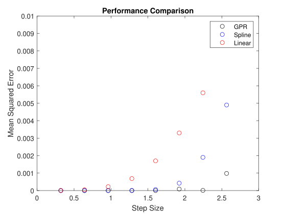
(a) MSE Error

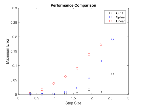
(b) MAX Error

Figure 1: Performance Comparison in the Uniform case

In this case, GPR is shown to outperform both interpolating spline methods.

4.2 Case II

Next, we consider the following non-uniform grid. The grid $G\subset\mathcal{M}$ is:

$G=[-4.36,-4.04,-2.44,1.73,2.05,4.94,5.26,8.14,9.10]$

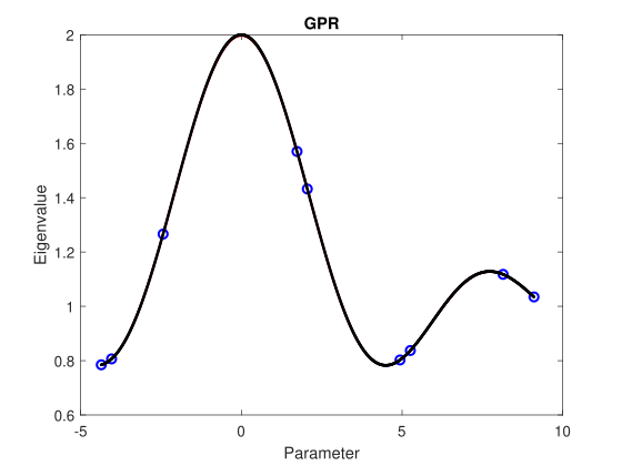
(a) GPR

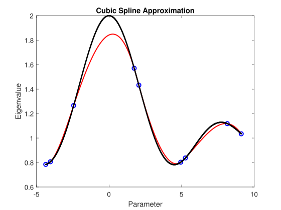
(b) Cubic spline interp.

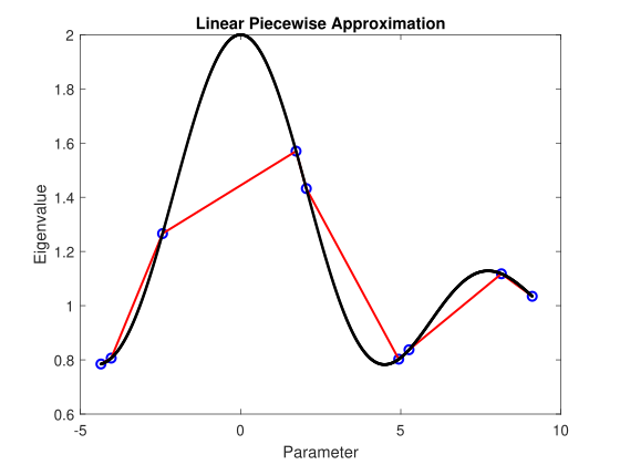
(c) Linear piecewise interp.

Figure 2: Comparison between the function $f(\mu)$ (black) and estimates using three different methods. Blue circles are the training data points.

Due to non-uniformity, some interpolation methods cannot be used. Furthermore, one doesn’t expect that the error using spline methods will approach zero for denser but non-uniform grids. GPR, on the other hand, performs fairly well, as can be seen in Figure 2. In particular, it is able to estimate better regions when the second derivative is the largest.

5 Numerical results

In this section, we present the numerical results of some eigenvalue problems using the GPR model with different covariance functions. We consider five eigenvalue problems. In order to compare the results using GPR with different covariance functions, we calculate the eigenvalues on a set of test points $\mu_{tst}$ and reported the relative root mean squared error(RRMSE) defined as

$$RRMSE=\sqrt{\frac{\frac{1}{n_{t}}\sum\limits_{i=1}^{n_{t}}(\lambda_{i}-\hat{\lambda}_{i})^{2}}{\sum\limits_{i=1}^{n_{t}}\lambda_{i}^{2}}},$$

where $\lambda_{i}$ and $\hat{\lambda}_{i}$ are the FEM and GPR based eigenvalues respectively and $n_{t}$ denote the number of test points. Also, the eigenvalues using GPR and FEM are presented for four selected test points and the corresponding relative error for each problem. In our experiments, we assume that the mean is linear.

Example 1

Let us consider the following eigenvalue problem

$$\left\{\begin{array}[]{ll}-\nabla\cdot(A(\mu)\nabla u(\mu))&=\lambda(\mu)u\quad\text{in}\quad\Omega=[-1,1]^{2}\\ u(\mu)=0&\textrm{ on }\partial\Omega\end{array}\right.$$ (5)

with the matrix $A(\mu)=\begin{bmatrix}1&0\\ 0&1+\mu\end{bmatrix}$, where we choose the parameter space as $\mathcal{M}=[-0.9,0.9]$. The exact solution is known for this problem. The eigenvalues and eigenvectors are given by

$$\lambda_{m,n}(\mu)=\frac{\pi^{2}}{4}(m^{2}+(1+\mu)n^{2})$$

$$u_{m,n}=cos(\frac{m\pi}{2}x)cos(\frac{n\pi}{2}y),\quad\forall m,n\in\mathbb{N}.$$

The first six eigenvalues of the problem are plotted in Figure 3. Note that graph of the first eigenvalue is separated from the others but other graphs of the eigenvalues have crossings. For the numerical results, we use the training points $\mu_{tr}=-0.9:0.1:0.9$ and test points are $\mu_{tst}=-0.9:0.05:0.9$.

In Figure 4, we have shown the GPR for the first eigenvalue of the EVP (5) using four different covariance functions/kernels. All the GPRs are shown in Figure 4 and they look the same. The first eigenvalues at four test points $\mu=-0.75,-0.25,0.25,0.75$ are reported in Table 1. For all four cases, the eigenvalues are exactly the same.

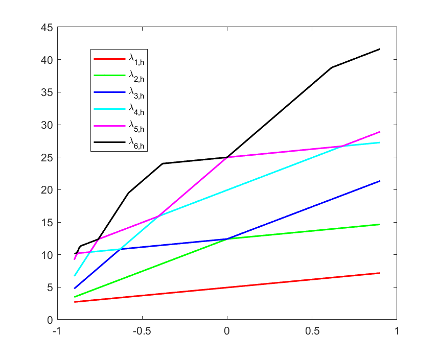
Figure 3: First six eigenvalues of EVP (5).

(a) Exp Kernel

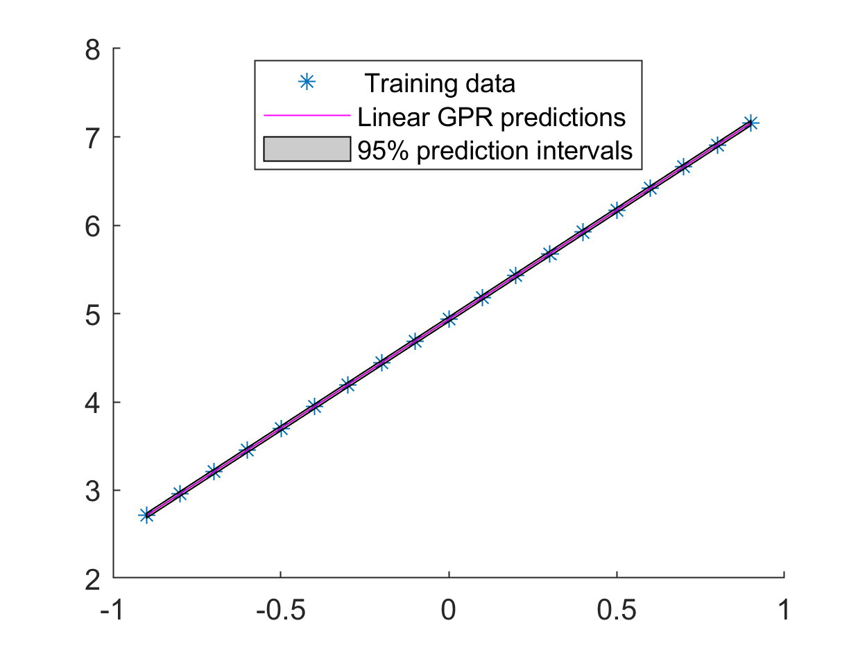
(b) Matern 3/2 Kernel

(c) Matern 5/2 Kernel

(d) SE Kernel

Figure 4: GPR corresponding to 1st eigenvalues of EVP (5) using different kernels.

Cov	Method	$\mu=-0.75$	$\mu=-0.25$	$\mu=0.25$	$\mu=0.75$
	FEM	3.08453581	4.31835348	5.55216884	6.78598322
Exp	GPR	3.08453660	4.31835243	5.55216826	6.78598409
Matern 3/2	GPR	3.08453660	4.31835243	5.55216826	6.78598409
Matern 5/2	GPR	3.08453660	4.31835243	5.55216826	6.78598409
SE	GPR	3.08453660	4.31835243	5.55216826	6.78598409

Table 1: Comparison of 1st eigenvalues of (5) using GPR model with different covariance functions.

In Figure 5, we have shown the GPR for the second eigenvalues of the EVP (5) using four different covariance functions with a 95 percent confidence interval. The second eigenvalues are compared at the four test points $\mu=-0.75,-0.25,0.25,0.75$, and the relative error between the FEM solution and GPR-based data-driven models are reported in Table 2. To measure the performance of the GPR with different covariance functions, we report RRMSE calculated using the test set $\mu_{tst}=-0.9:0.05:0.9$ in the last column of Table 2. Clearly, the GPR with exponential covariance function is better than the other three. Note that the GP with the exponential kernel is only continuous. The confidence interval for the exponential kernel shows the correct behavior because the interval is narrow where the training data and test data coincide and the interval is large where the test data is not in the training set. The confidence interval corresponding to the other covariance kernel is almost the same in all test data. From the MSE, one can conclude that the GPR with exponential kernels is giving better results than others.

Since the graph of the second eigenvalues has two segments that means it comes from two different analytical solutions. Because the eigenvectors are parameter independent, there are only two independent columns of the snapshot matrix. Hence there are only two reduced co-efficient for the second eigenvectors. In Figure 6-Figure 7, we have plotted the GPR for the coefficients corresponding to the second eigenvector. One can see that the confidence interval corresponding to the exponential covariance function behaves better than the rest. In Figure 8, we have shown the error between the second eigenvector obtained by FEM and the second eigenvectors using GPR with different kernels at $\mu=-0.75$. From the figure, we can see that the error for the exponential one is of order $10^{-4}$ whereas the error is of order $10^{-3}$ for the squared exponential kernel.

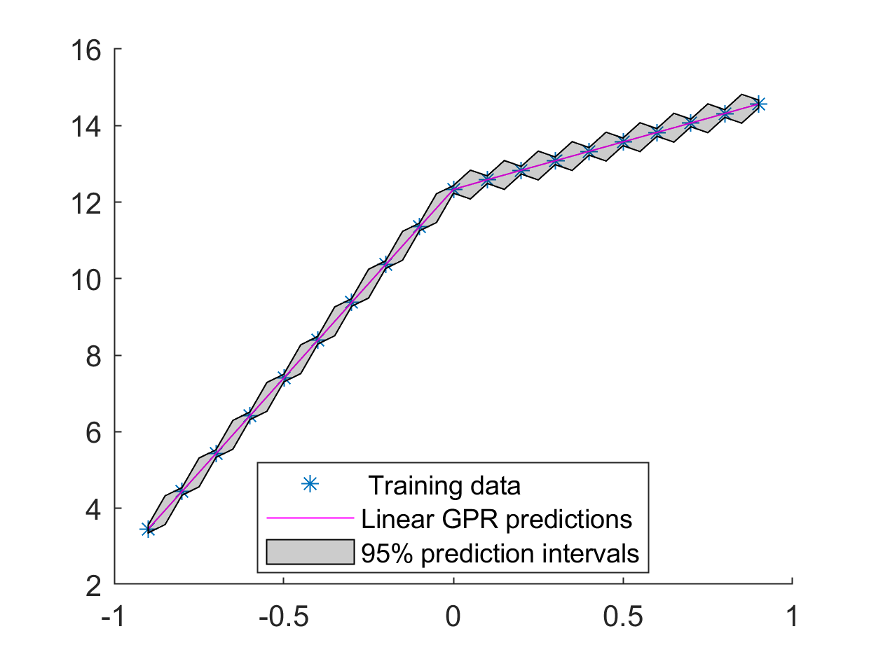
(a) Exp Kernel

(b) Matern 3/2 Kernel

(c) Matern 5/2 Kernel

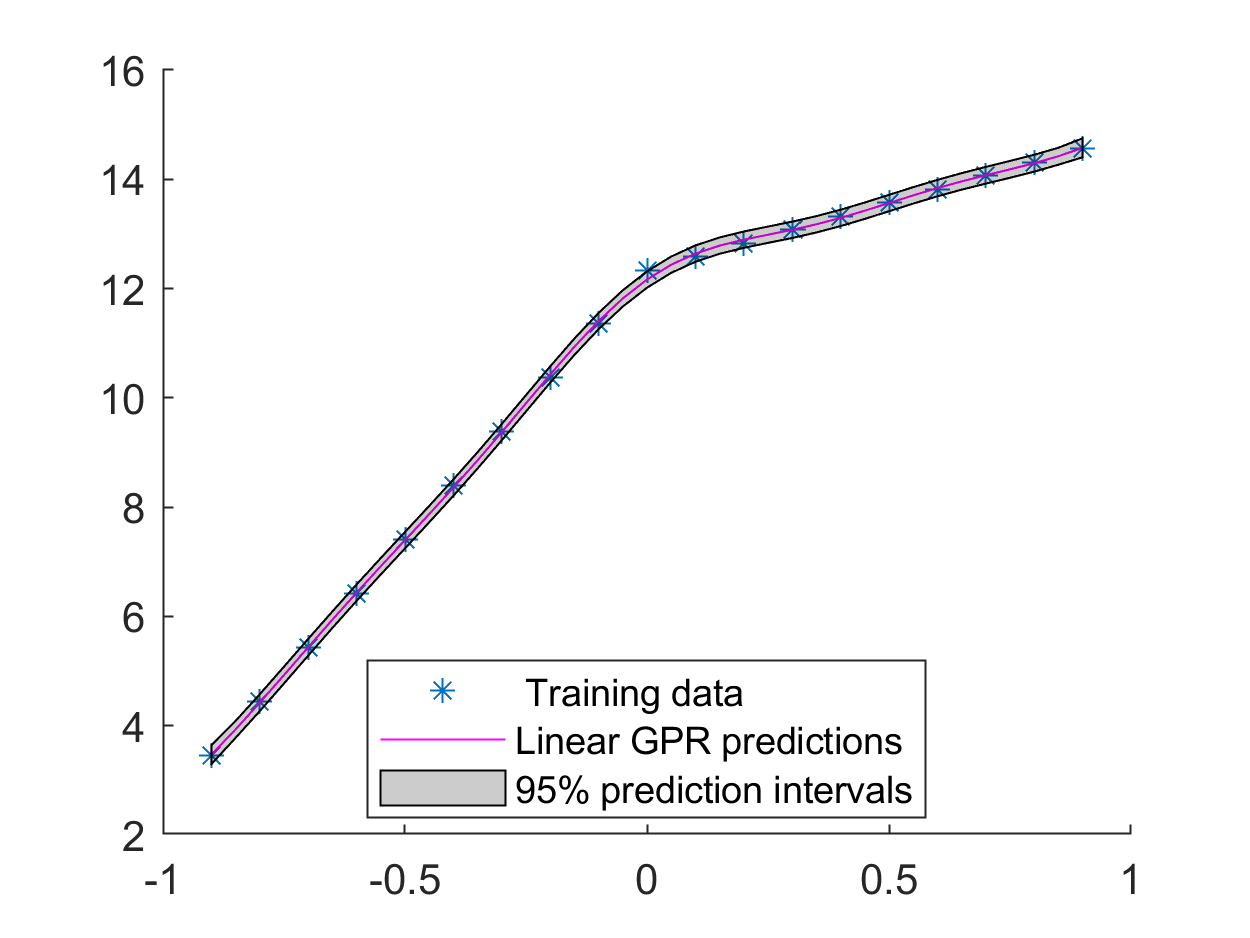
(d) SE Kernel

Figure 5: GPR corresponding to 2nd eigenvalues of EVP (5) using different kernels.

Cov	Method	$\mu=-0.75$	$\mu=-0.25$	$\mu=0.25$	$\mu=0.75$	RRMSE
	FEM	4.93615339	9.87196392	12.95691963	14.19104350
Exp	GPR	4.93617312	9.87118176	12.95613751	14.19106357	$2.7\times 10^{-5}$
	Rel. Err.	$3.9\times 10^{-6}$	$7.9\times 10^{-5}$	$6.0\times 10^{-5}$	$1.4\times 10^{-6}$
Matern 3/2	GPR	4.93530638	9.87008026	12.95503589	14.19019650	$2.1\times 10^{-4}$
	Rel. Err.	$1.7\times 10^{-4}$	$1.9\times 10^{-4}$	$1.4\times 10^{-4}$	$5.9\times 10^{-5}$
Matern 5/2	GPR	4.93251265	9.86655306	12.95150837	14.18740285	$3.4\times 10^{-4}$
	Rel. Err.	$7.3\times 10^{-4}$	$5.4\times 10^{-4}$	$4.1\times 10^{-4}$	$2.5\times 10^{-4}$
SE	GPR	4.92706677	9.90066863	12.98562341	14.18195696	$6.2\times 10^{-4}$
	Rel. Err.	$1.8\times 10^{-3}$	$2.9\times 10^{-3}$	$2.2\times 10^{-3}$	$6.4\times 10^{-4}$

Table 2: Comparision of 2nd eigenvalues of (5) using GPR model with different covariance functions.

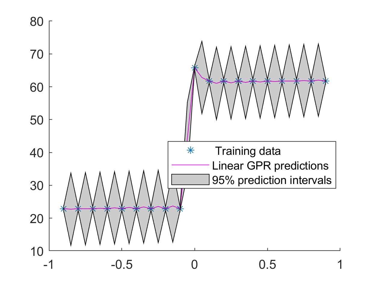
(a) Exp Kernel

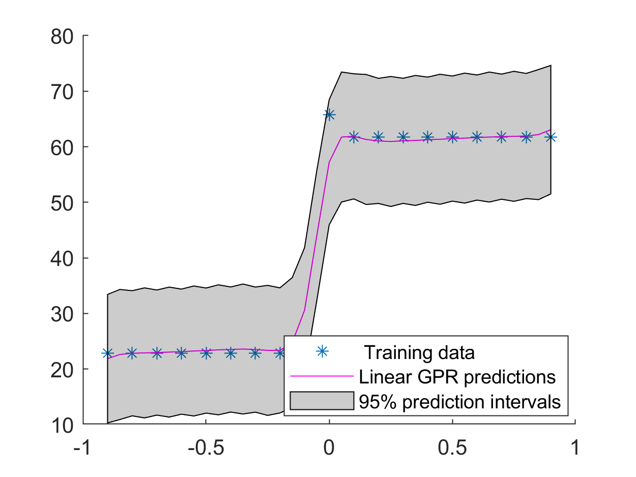
(b) Matern 3/2 Kernel

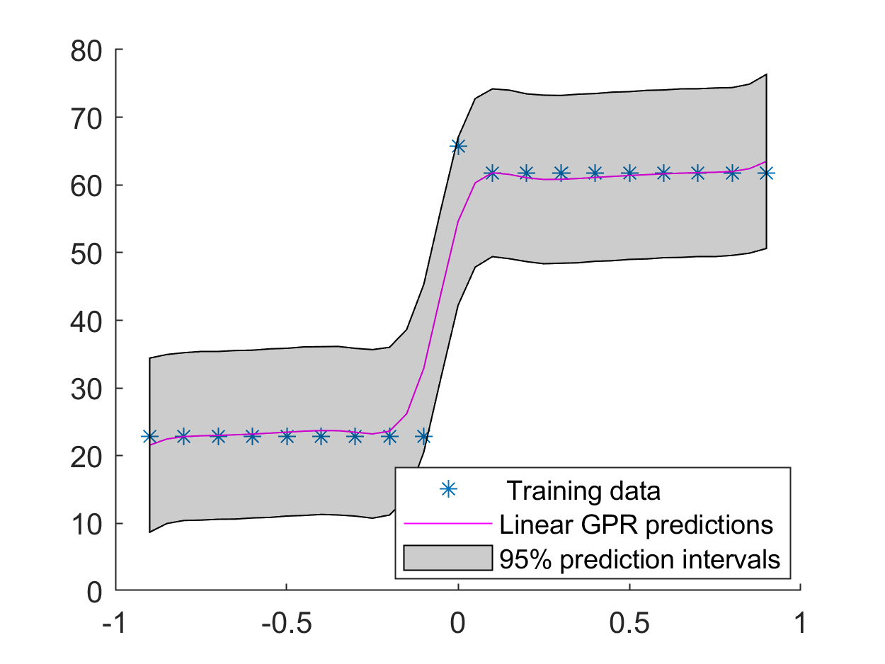
(c) Matern 5/2 Kernel

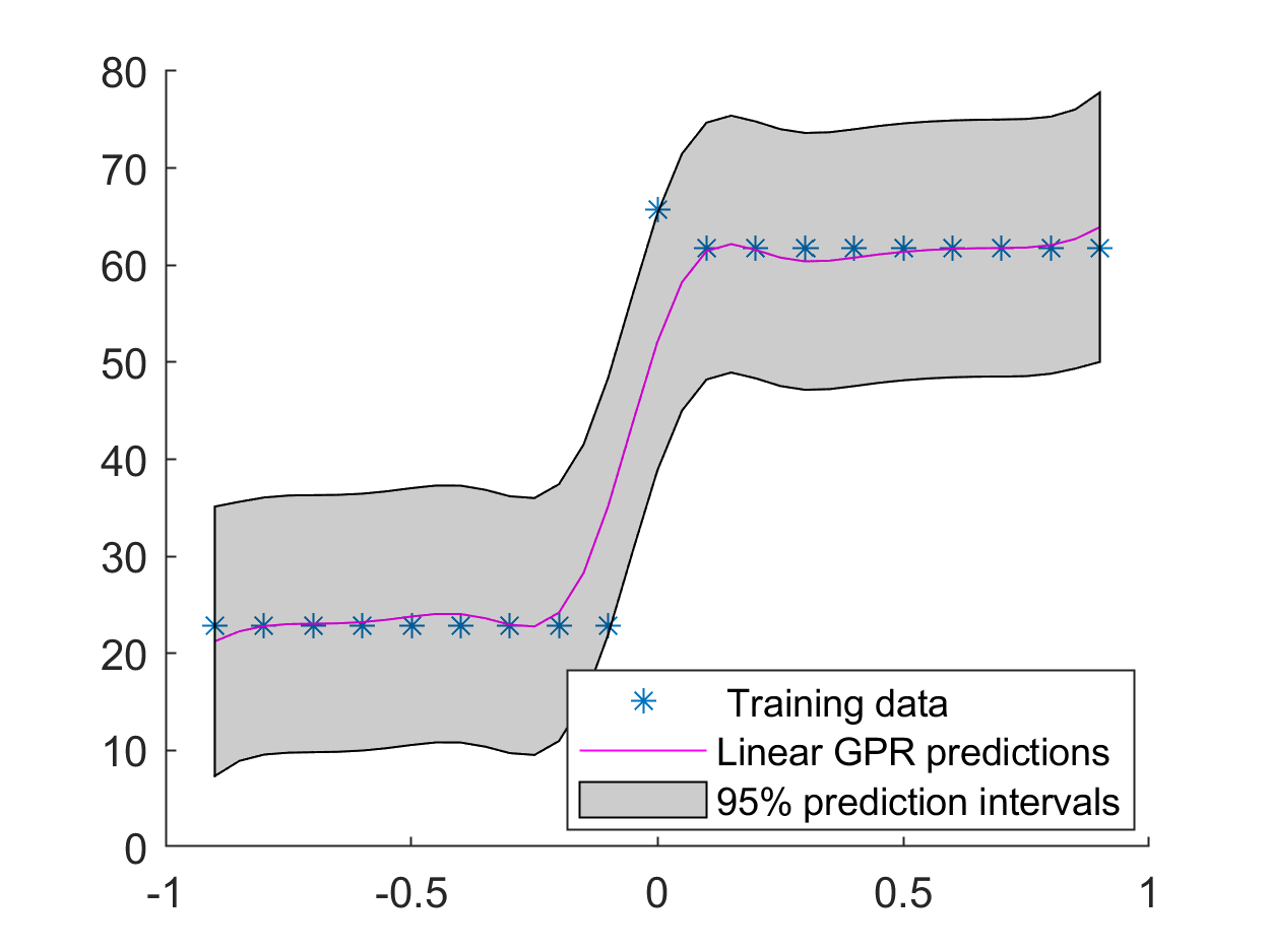
(d) Squared Exponential Kernel

Figure 6: GPR corresponding to 1st coefficient of the reduced 2nd eigenvector of EVP (5) using different kernels.

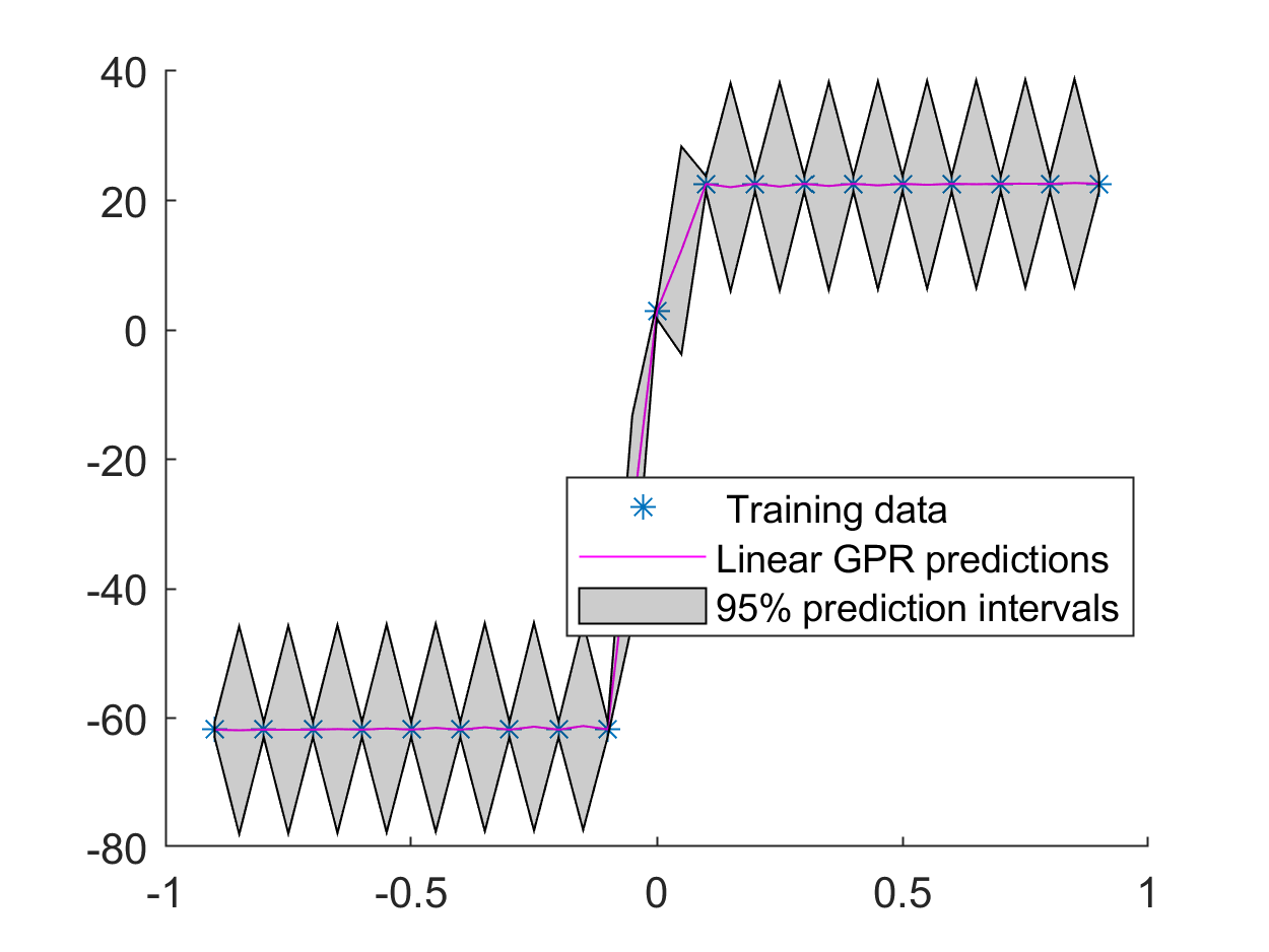
(a) Exp Kernel

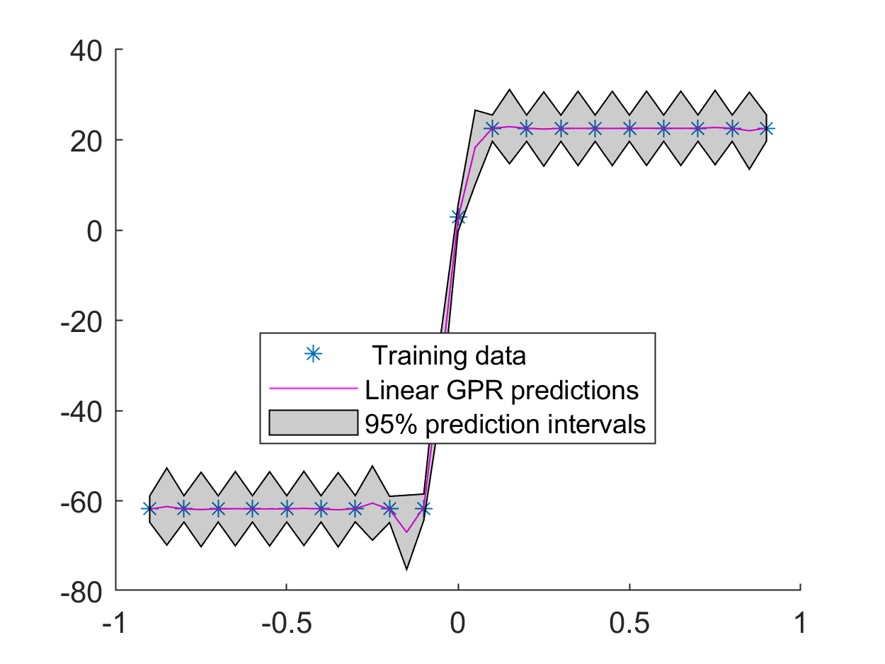
(b) Matern 3/2 Kernel

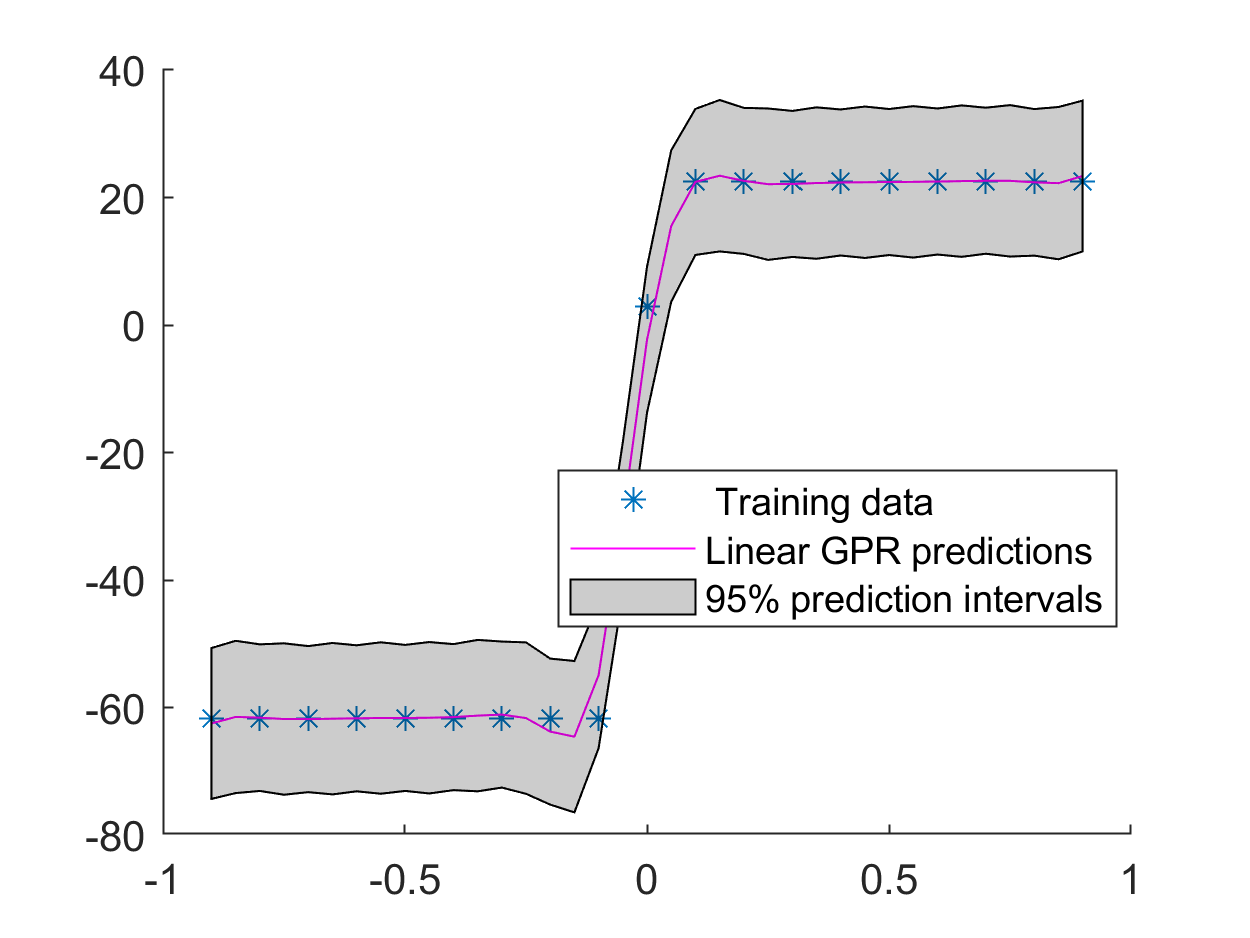
(c) Matern 5/2 Kernel

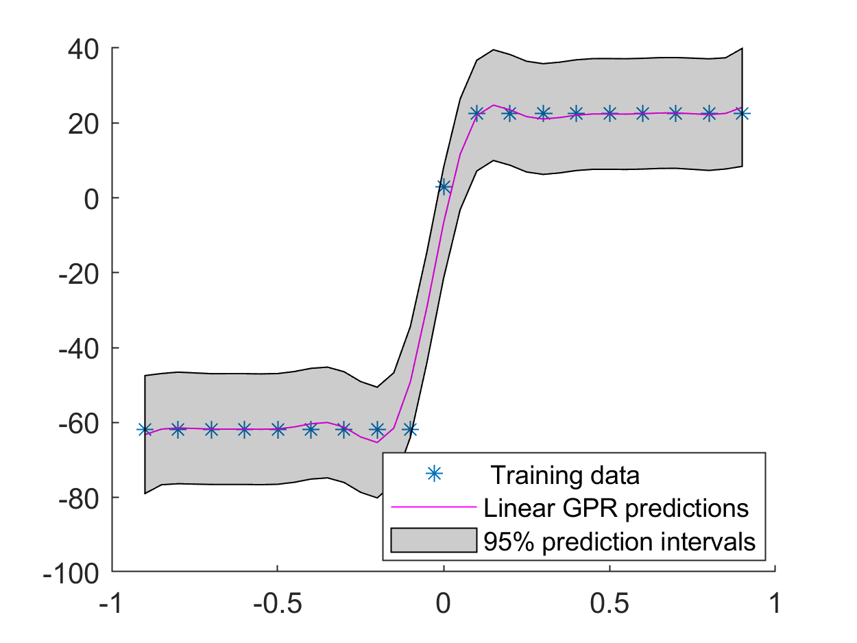
(d) SE Kernel

Figure 7: GPR corresponding to 2nd coefficient of the Reduced 2nd eigenvector of EVP (5) using different kernels.

(a) Exp Kernel

(b) Matern 3/2 Kernel

(c) Err Matrn 5/2 Kernel

(d) SE Kernel

Figure 8: Error between the FEM and GPR based 2nd eigenvectors of EVP (5) using different kernels at ${\mu}=-0.75$.

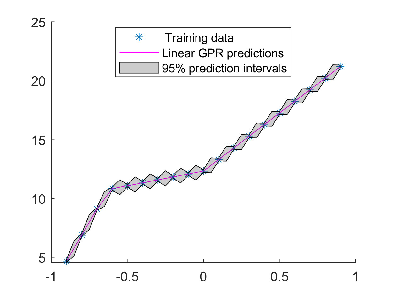
(a) Exp Kernel

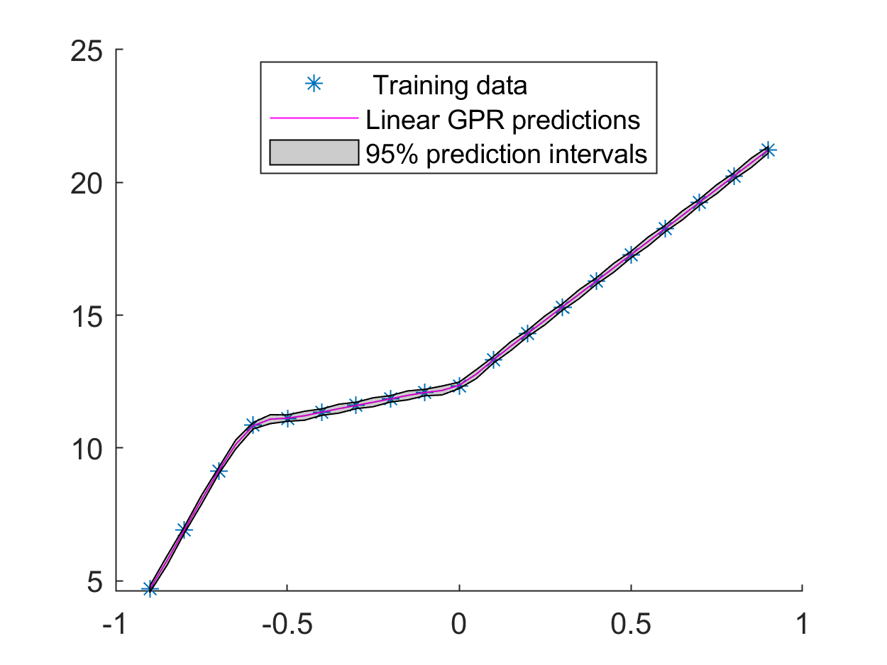
(b) Matern 3/2 Kernel

(c) Matern 5/2 Kernel

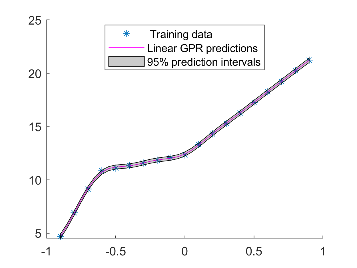
(d) SE Kernel

Figure 9: GPR corresponding to 3rd eigenvalues of EVP (5) using different kernels.

In Figure 9, we have shown the GPR with the 95 percent interval of confidence for the third eigenvalues of the EVP (5) using four different covariance functions. The 3rd eigenvalues are compared at the four test points $\mu=-0.75,-0.25,0.25,0.75$. The relative error between the FEM solution and the GPR-based data-driven model is reported in Table 3. From RRMSE we can see that all models with four different covariance functions give comparable results. Since the graph of the three eigenvalues has three segments so there are only three reduced coefficients corresponding to the third eigenvectors. In Figure 10-Figure 12, we have plotted the GPR for the coefficients corresponding to the third eigenvector. One can see that the confidence interval corresponding to the exponential covariance function behaves better than the rest. The mean of the GPR with exponential kernel fits the data pretty well but the others don’t. In Figure 13, we have shown the error between the third eigenvector obtained by FEM and the second eigenvectors using GPR with different kernels at $\mu=-0.75$. From the figure, we can see that the error for the exponential one is of order $10^{-3}$ whereas the error is of order $10^{-2}$ for the squared exponential kernel. Although the eigenvalues give comparable results the eigenvector is better for the GPR with the exponential kernel.

Cov	Method	$\mu=-0.75$	$\mu=-0.25$	$\mu=0.25$	$\mu=0.75$	RRMSE
	FEM	8.02390130	11.72278922	14.80775895	19.74354759
Exp	DD	8.01681993	11.72010757	14.81133226	19.74424881	$5.0\times 10^{-4}$
	Rel. Err.	$8.8\times 10^{-4}$	$2.2\times 10^{-4}$	$2.4\times 10^{-4}$	$3.5\times 10^{-5}$
Matern 3/2		8.04708228	11.72079767	14.80636031	19.74370150	$3.3\times 10^{-4}$
	Rel. Err.	$2.9\times 10^{-3}$	$1.6\times 10^{-4}$	$9.4\times 10^{-5}$	$7.7\times 10^{-6}$
Matern 5/2		8.05908664	11.72952729	14.81238949	19.74355679	$4.0\times 10^{-4}$
	Rel. Err.	$4.4\times 10^{-3}$	$5.7\times 10^{-4}$	$3.1\times 10^{-4}$	$4.6\times 10^{-7}$
SE	DD	8.09465668	11.74541561	14.83245776	19.74165644	$5.9\times 10^{-4}$
	Rel. Err.	$8.8\times 10^{-3}$	$1.9\times 10^{-3}$	$1.7\times 10^{-3}$	$9.5\times 10^{-5}$

Table 3: Comparison of 3rd eigenvalues of (5) using GPR model with different covariance functions.

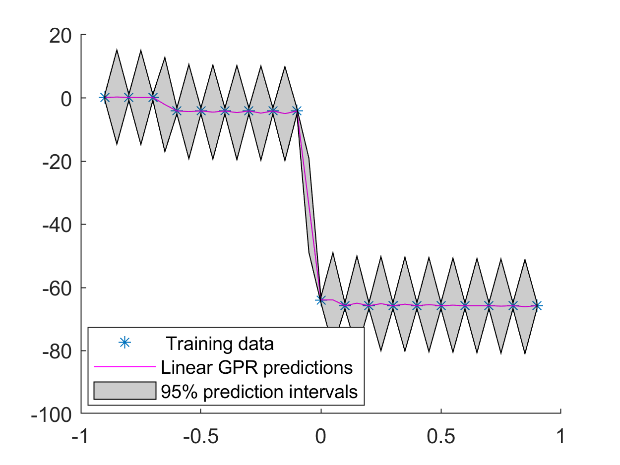
(a) Exp Kernel

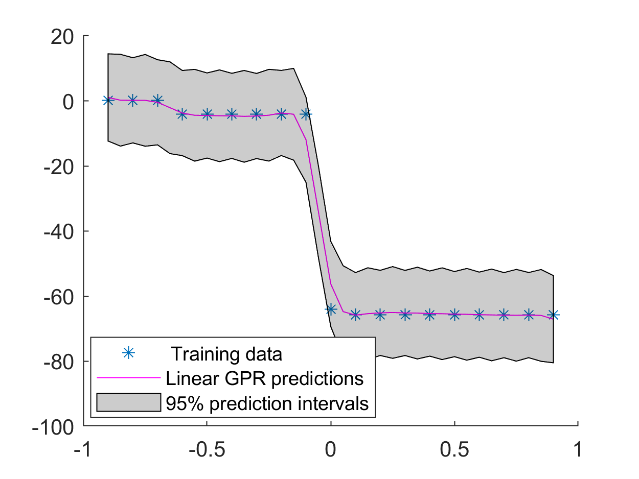
(b) Matern 3/2 Kernel

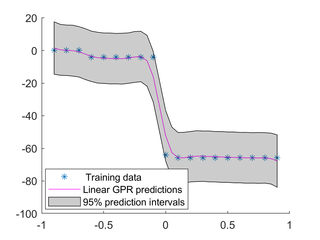
(c) Matern 5/2 Kernel

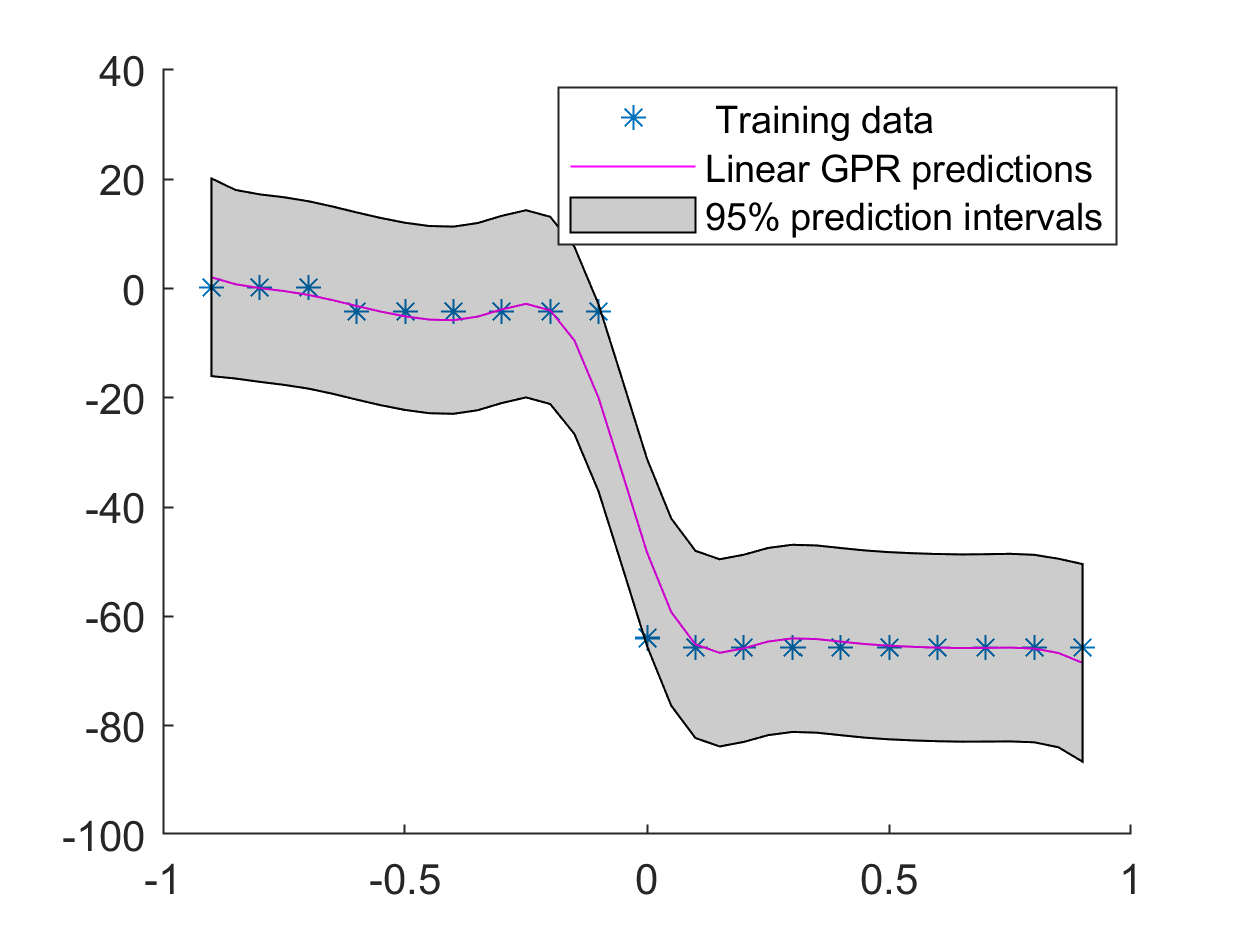
(d) SE Kernel

Figure 10: GPR corresponding to 1st coefficient of the Reduced 3rd eigenvector of EVP (5) using different kernels.

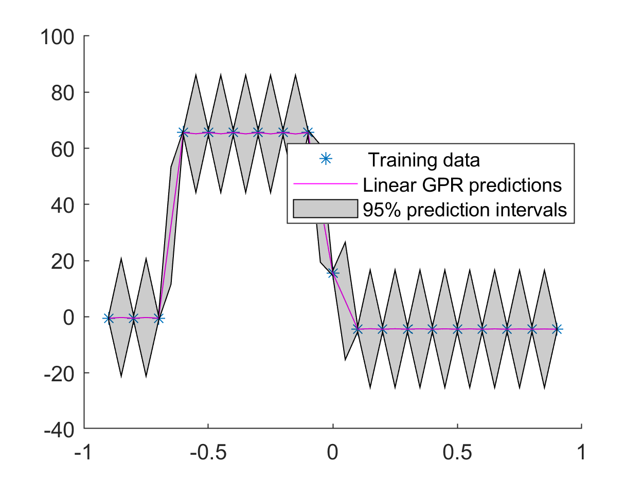
(a) Exp Kernel

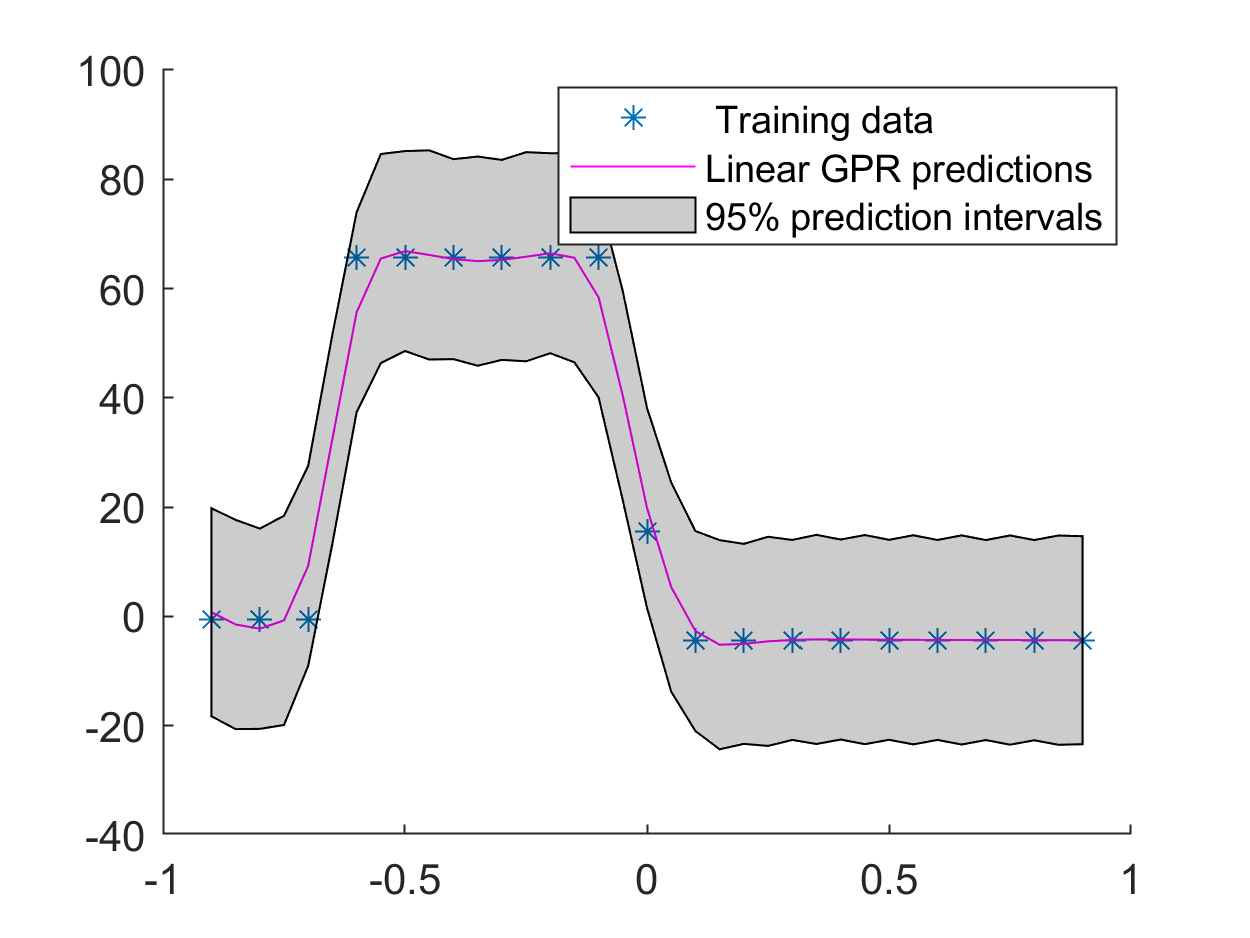
(b) Matern 3/2 Kernel

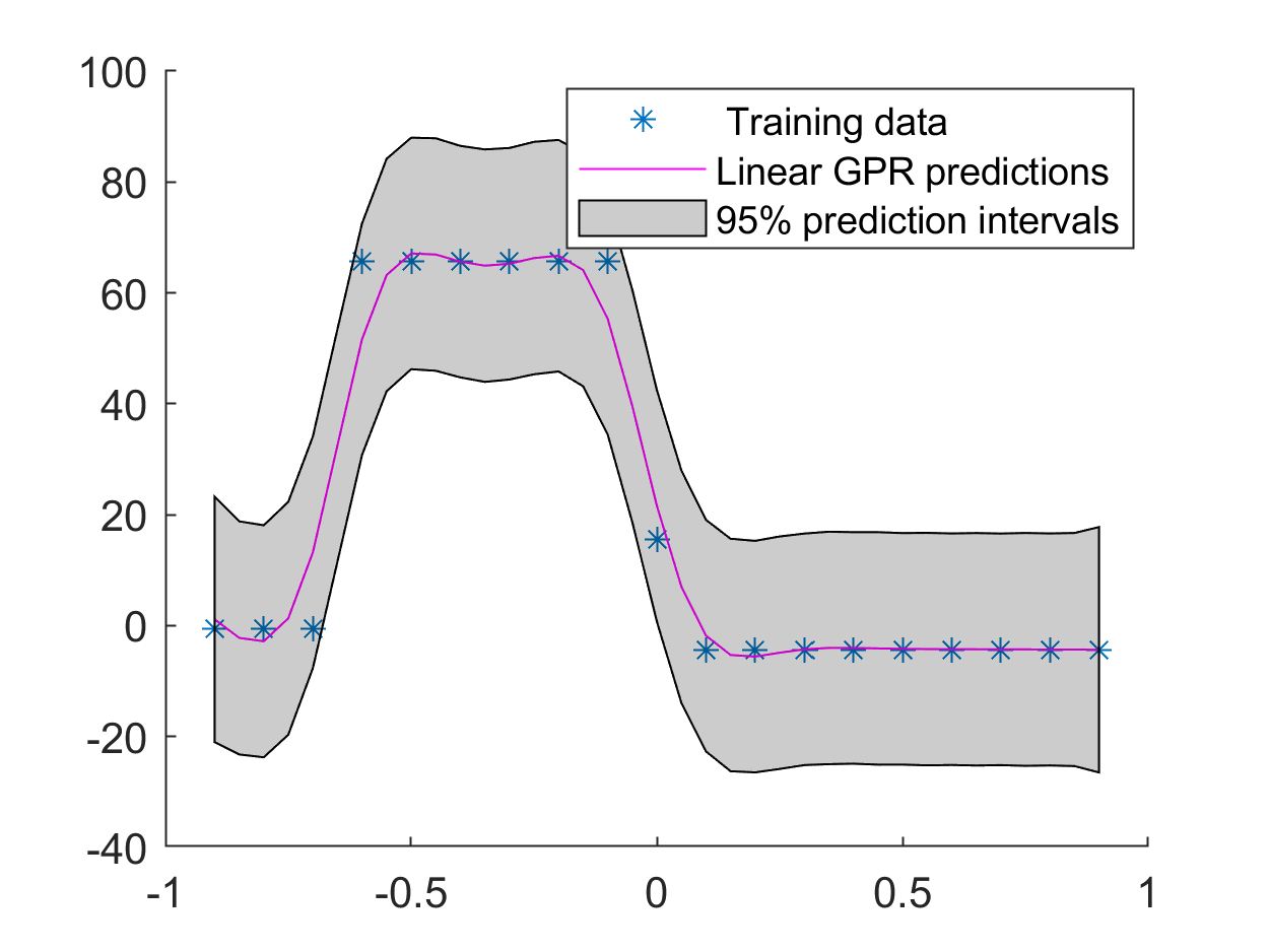
(c) Matern 5/2 Kernel

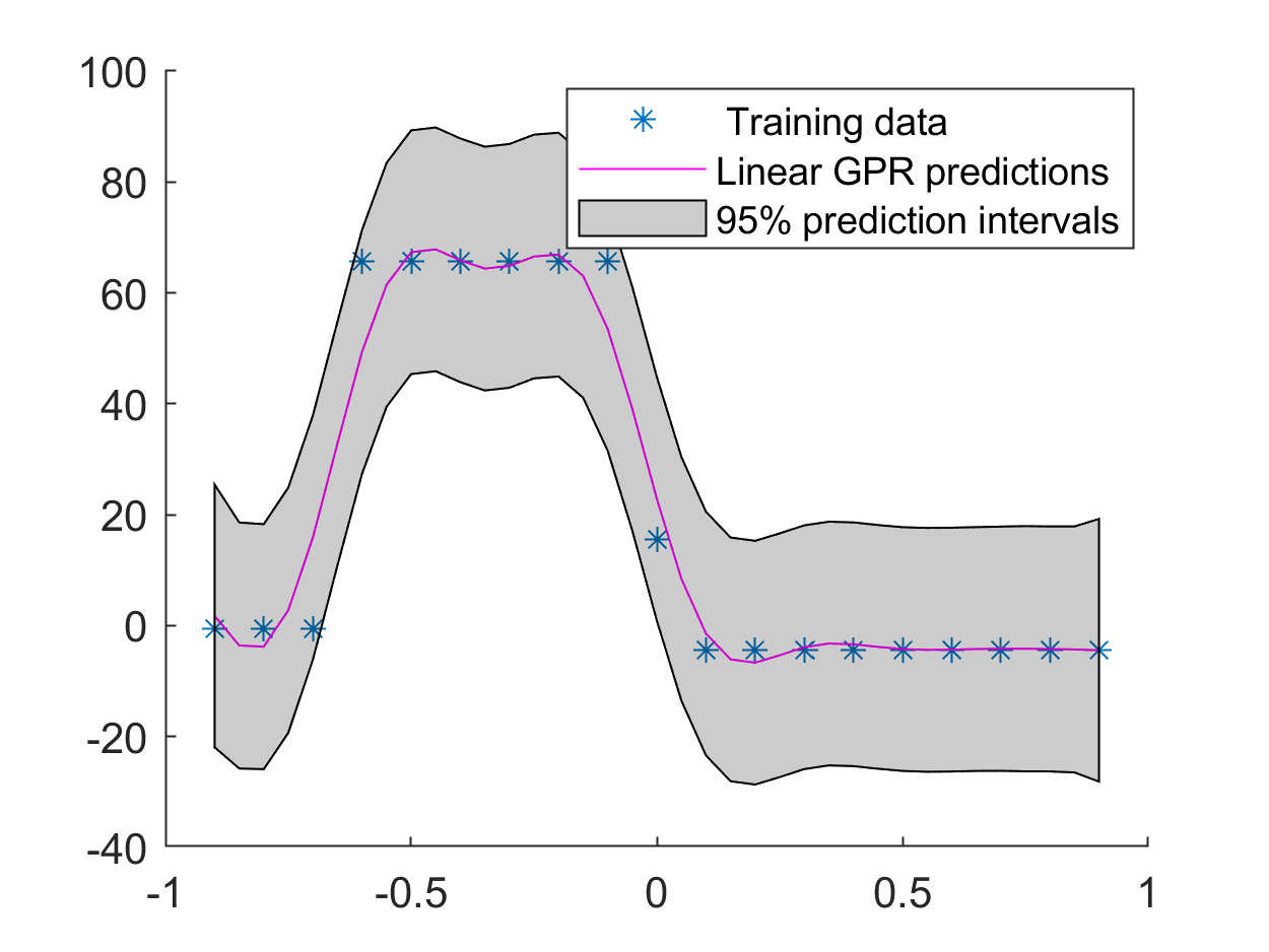
(d) SE Kernel

Figure 11: GPR corresponding to 2nd coefficient of the Reduced 3rd eigenvector of EVP (5) using different kernels.

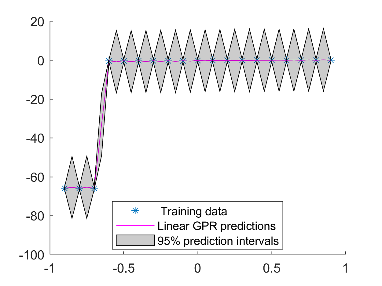
(a) Exp Kernel

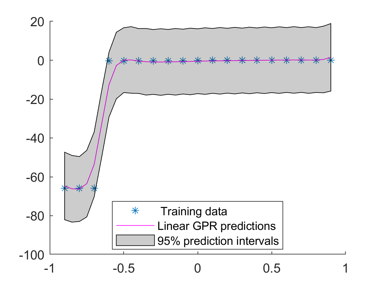
(b) Matern 3/2 Kernel

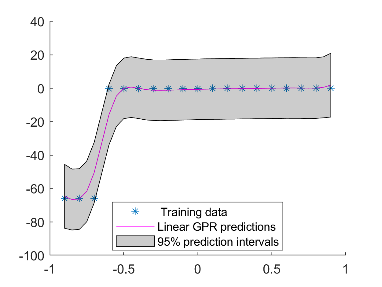
(c) Matern 5/2 Kernel

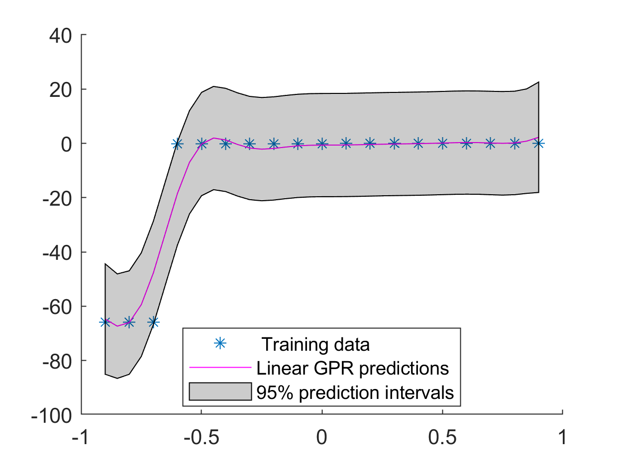
(d) SE Kernel

Figure 12: GPR corresponding to 3rd coefficient of the Reduced 3rd eigenvector of EVP (5) using different kernels.

(a) Exp Kernel

(b) Matern 3/2 Kernel

(c) Err Matrn 5/2 Kernel

(d) SE Kernel

Figure 13: Error between the FEM and GPR-based third eigenvectors of EVP (5) using different kernels at $\mu=-0.75$.

Example 2

Let us consider the eigenvalue problem defined on $\Omega=\left(-\frac{\pi}{2},\frac{\pi}{2}\right)^{2}\subset\mathbb{R}^{2}$

$$\left\{\begin{aligned} &-\frac{1}{2}\Delta u(x,y)+\frac{1}{2}\mu^{2}(x^{2}+y^{2})u(x,y)=\lambda u(x,y)&&\text{in }\Omega\\ &u=0&&\text{on }\partial\Omega\end{aligned}\right.$$ (6)

The analytic eigenvalues and eigenvectors of this problem are given by

$$\lambda_{m,n}(\mu)=(m+n+1)\mu$$

$$u_{m,n}(x,y;\mu)=\frac{1}{\sqrt{2^{m+n}m!n!\pi}}e^{-\mu(x^{2}+y^{2})/2}H_{m}(\sqrt{\mu}x)H_{n}(\sqrt{\mu}y)$$

for $m,n=0,1,2,3,\dots$, where $H_{n}$ is the Hermite polynomial of order $n$. For the numerical purpose, we choose parameter space $\mathcal{M}=[1,9].$ The parameters used for training are $\mu_{tr}=1:0.4:9$ and test points are $\mu_{tst}=1:0.2:9$. The first four eigenvalues are shown in Figure 14. Note that this problem has repeated eigenvalues.

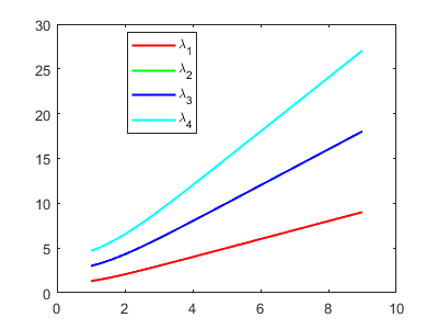
Figure 14: First four eigenvalues of the EVP (6).

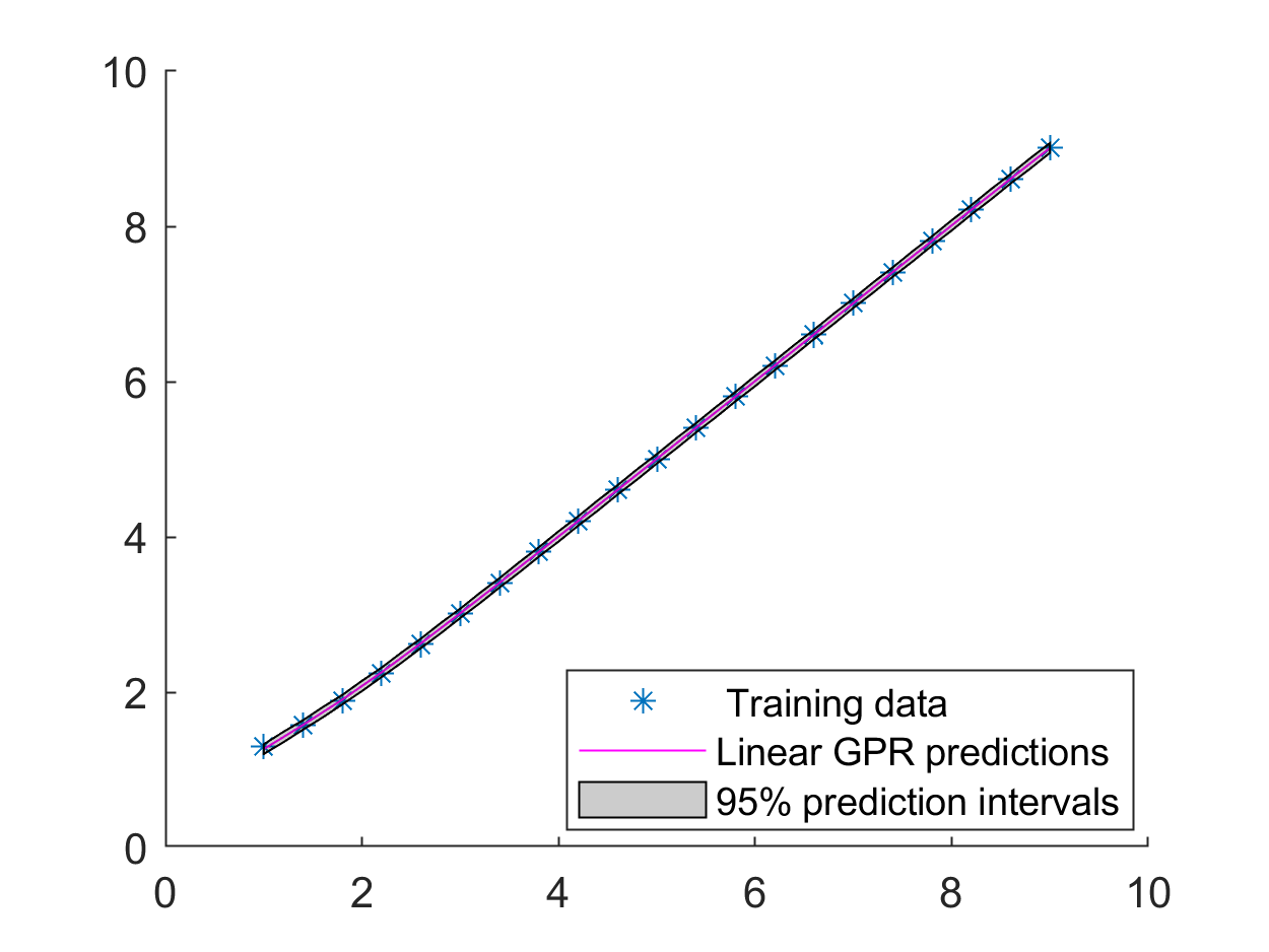
(a) Exp Kernel

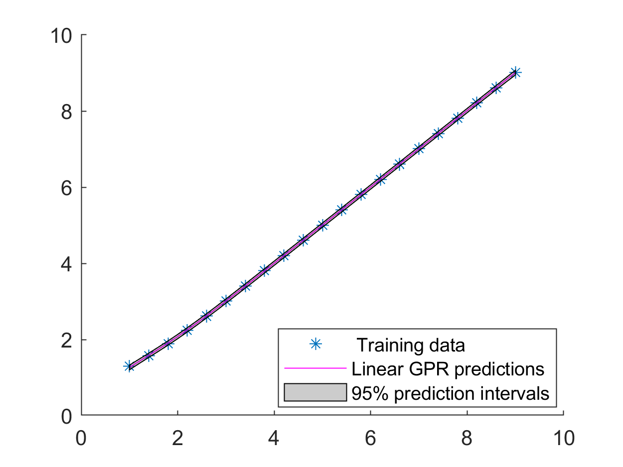
(b) Matern 3/2 Kernel

(c) Matern 5/2 Kernel

(d) SE Kernel

Figure 15: GPR corresponding to 1st eigenvalues of EVP (6) using different kernels.

In Figure 15, we have shown the GPR with the 95 percent confidence interval for the first eigenvalues of the EVP (6) using four different covariance functions. The first and second eigenvalues at four test points $\mu=1.6,3.6,5.6,7.6$ and the relative error are reported in Table 4 and Table 5 respectively. The RRMSE between the eigenvalues of the FEM and the GPR methods at the test set $\mu=1:0.2:9$ is reported in the last column of each table. The RRMSE is comparable but the RRMSE corresponding to the exponential kernel is a little better. In this case, we have six reduced coefficients corresponding to the first eigenvectors. In Figure 16-Figure 21, we have plotted the GPR for the coefficients corresponding to the first eigenvector. The confidence interval corresponding to the exponential kernel is more reliable than the others. The GPR for the sixth coefficient for the squared exponential kernel is not good. In Figure 22 and Figure 23, we have shown the error between the first and second eigenvector respectively obtained by FEM and the corresponding eigenvectors using GPR with different kernels at $\mu=1.6$. From Figure 23, we can see that the error for the exponential and SE is of order $10^{-3}$ whereas the error is of order $10^{-3}$ for Matern kernel.

Cov	Method	$\mu=1.6$	$\mu=3.6$	$\mu=5.6$	$\mu=7.6$	RRMSE
	FEM	1.72616800	3.60561533	5.60602312	7.61103552
Exp	GPR	1.74132712	3.60819316	5.60659938	7.61094426	$2.2\times 10^{-4}$
	Rel. Err	$8.8\times 10^{-3}$	$7.1\times 10^{-4}$	$1.0\times 10^{-4}$	$1.1\times 10^{-5}$
Matern 3/2	GPR	1.74621729	3.60446879	5.60623533	7.61161409	$2.3\times 10^{-4}$
	Rel. Err	$1.1\times 10^{-2}$	$3.1\times 10^{-4}$	$3.7\times 10^{-5}$	$7.6\times 10^{-5}$
Matern 5/2	GPR	1.74798302	3.60320721	5.60635034	7.61185640	$2.4\times 10^{-4}$
	Rel. Err	$1.2\times 10^{-2}$	$6.6\times 10^{-4}$	$5.8\times 10^{-5}$	$1.0\times 10^{-4}$
SE	GPR	1.74950736	3.59842117	5.60784680	7.61262827	$2.7\times 10^{-4}$
	Rel. Err	$1.3\times 10^{-2}$	$2.0\times 10^{-3}$	$3.2\times 10^{-4}$	$2.0\times 10^{-4}$

Table 4: Comparison of 1st eigenvalues of EVP (6) using GPR model with different covariance functions.

Cov	Method	$\mu=1.6$	$\mu=3.6$	$\mu=5.6$	$\mu=7.6$	RRMSE
	FEM	3.70472678	7.23116982	11.21378126	15.22421249
Exp	GPR	3.73063779	7.23659029	11.21459304	15.22425359	$1.7\times 10^{-4}$
	Rel. Err	$7.0\times 10^{-3}$	$7.4\times 10^{-4}$	$7.2\times 10^{-5}$	$2.6\times 10^{-6}$
Matern 3/2	GPR	3.73791051	7.22907869	11.21382739	15.22497608	$1.7\times 10^{-4}$
	Rel. Err	$9.0\times 10^{-3}$	$2.8\times 10^{-4}$	$4.1\times 10^{-6}$	$5.0\times 10^{-5}$
Matern 5/2	GPR	3.74097218	7.22612458	11.21422798	15.22543281	$1.9\times 10^{-4}$
	Rel. Err	$9.8\times 10^{-3}$	$6.9\times 10^{-4}$	$3.9\times 10^{-5}$	$8.0\times 10^{-5}$
SE	GPR	3.74268047	7.21515365	11.21953392	15.22609691	$2.3\times 10^{-4}$
	Rel. Err	$1.0\times 10^{-2}$	$2.2\times 10^{-3}$	$5.1\times 10^{-4}$	$1.2\times 10^{-4}$

Table 5: Comparison of 2nd eigenvalue of EVP (6) using GPR model with different covariance functions.

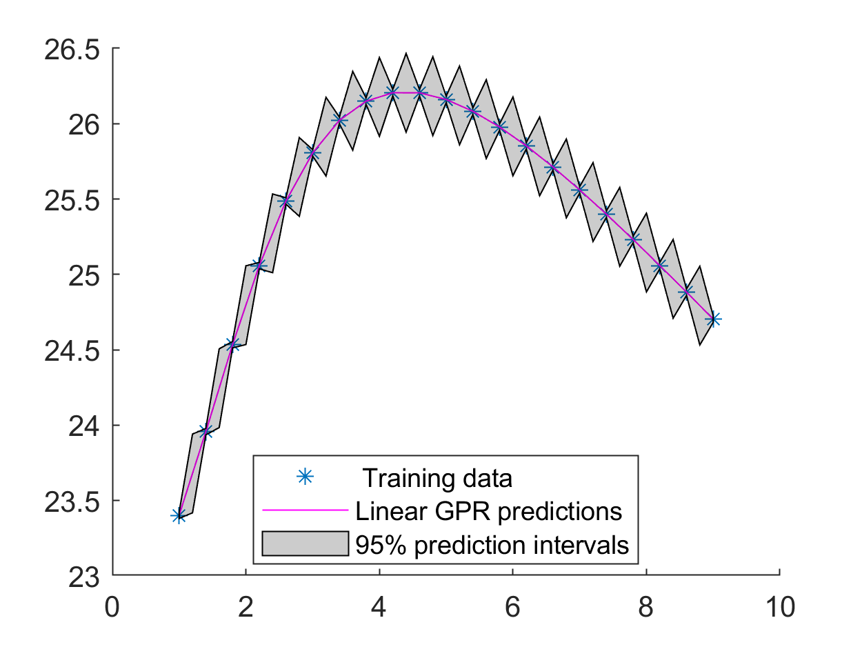
(a) Exp Kernel

(b) Matern 3/2 Kernel

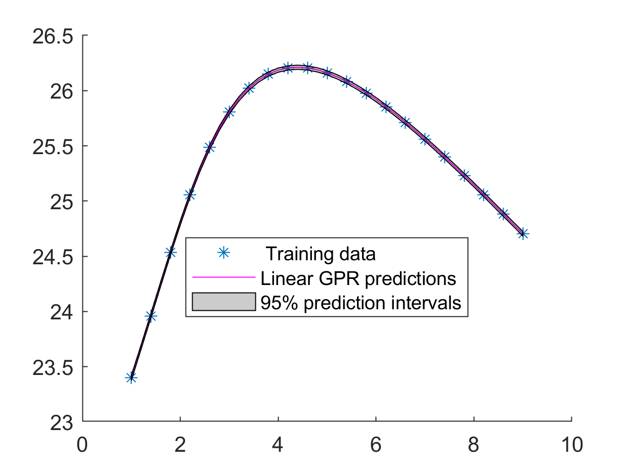
(c) Matern 5/2 Kernel

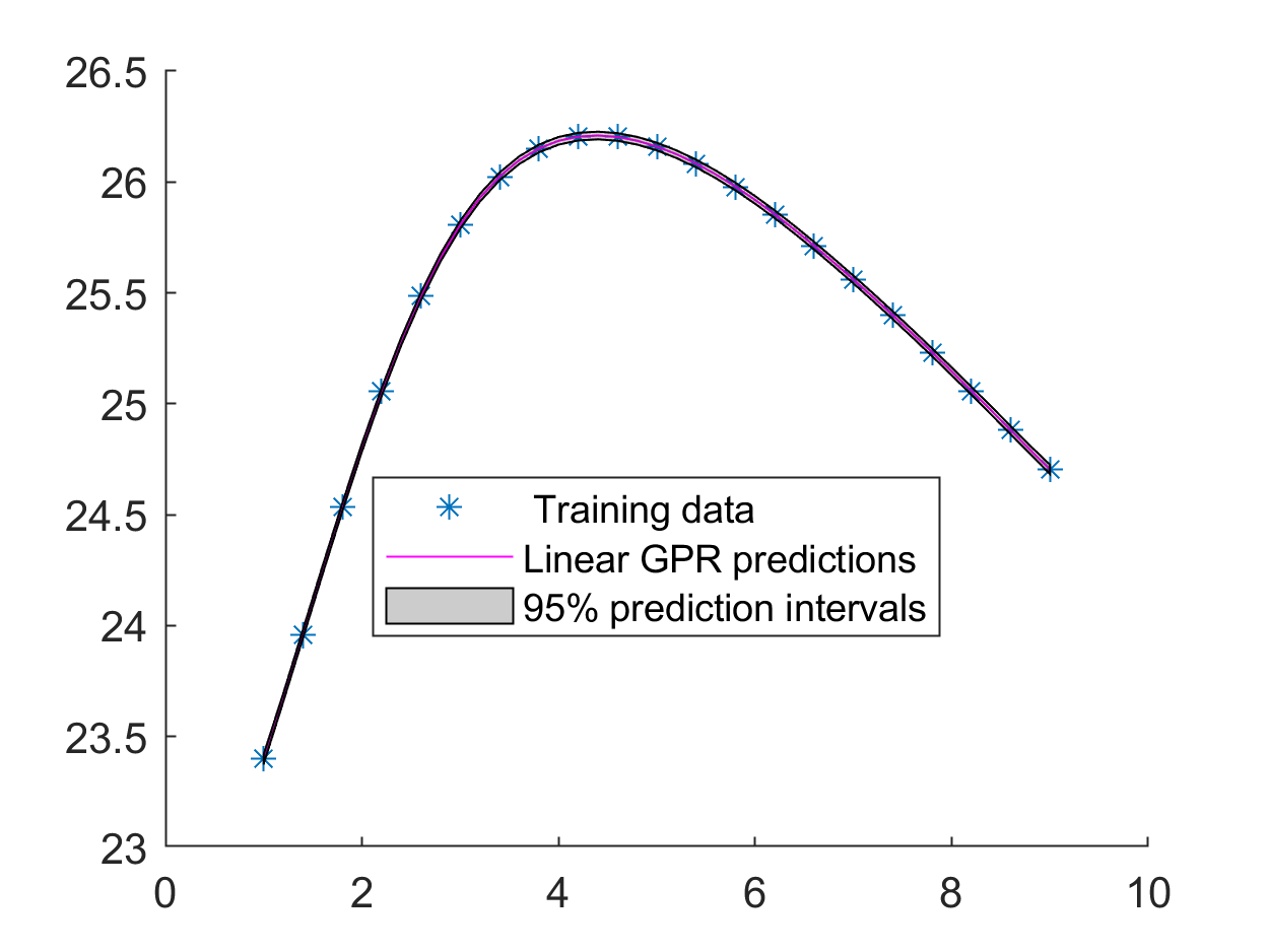
(d) SE Kernel

Figure 16: GPR corresponding to 1st coefficient of the reduced 1st eigenvector of EVP (6) using different kernels.

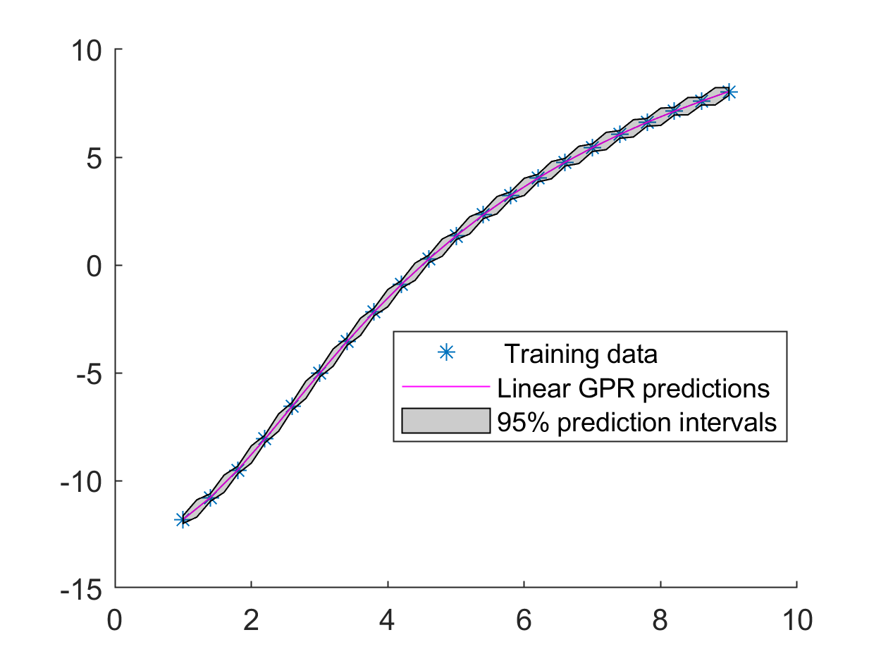
(a) Exp Kernel

(b) Matern 3/2 Kernel

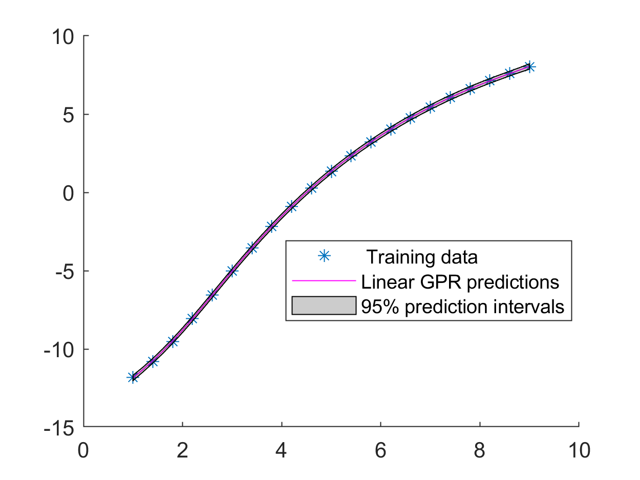
(c) Matern 5/2 Kernel

(d) SE Kernel

Figure 17: GPR corresponding to 2nd coefficient of the reduced 1st eigenvector of EVP (6) using different kernels.

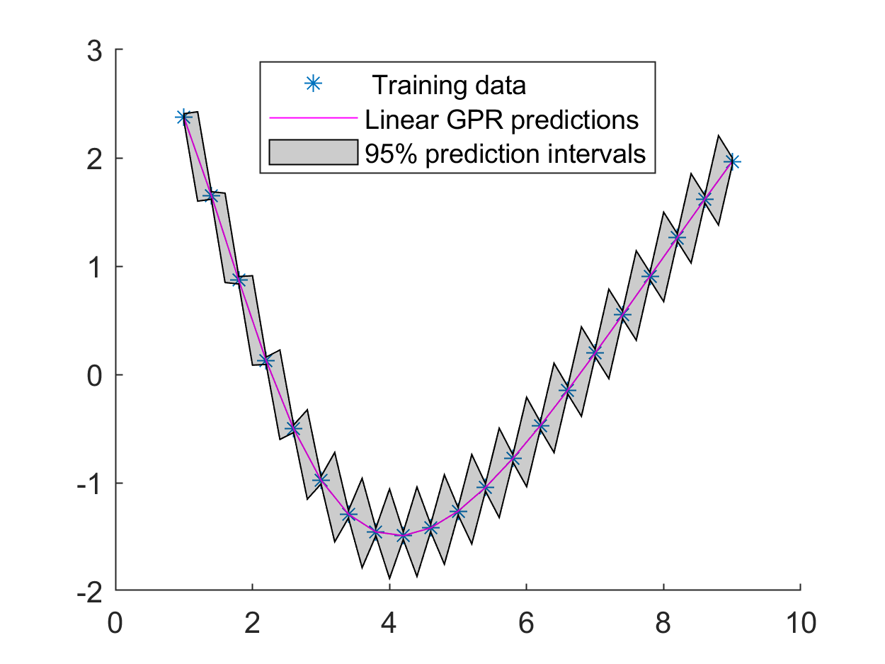
(a) Exp Kernel

(b) Matern 3/2 Kernel

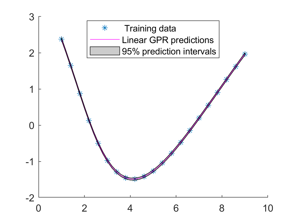
(c) Matern 5/2 Kernel

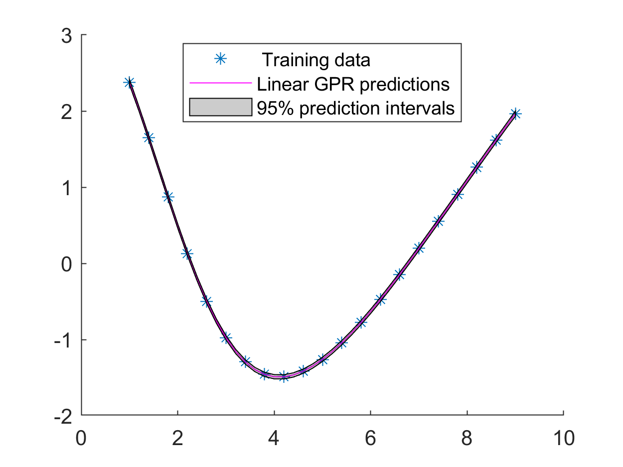
(d) SE Kernel

Figure 18: GPR corresponding to 3rd coefficient of the reduced 1st eigenvector of EVP (6) using different kernels.

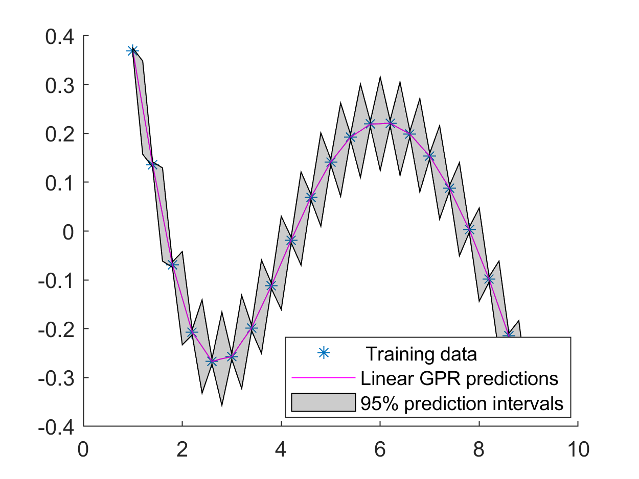
(a) Exp Kernel

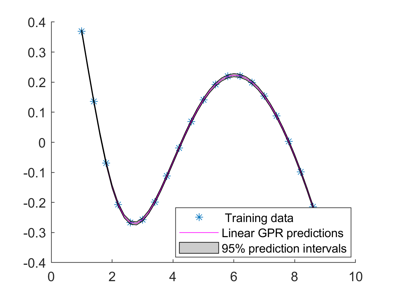
(b) Matern 3/2 Kernel

(c) Matern 5/2 Kernel

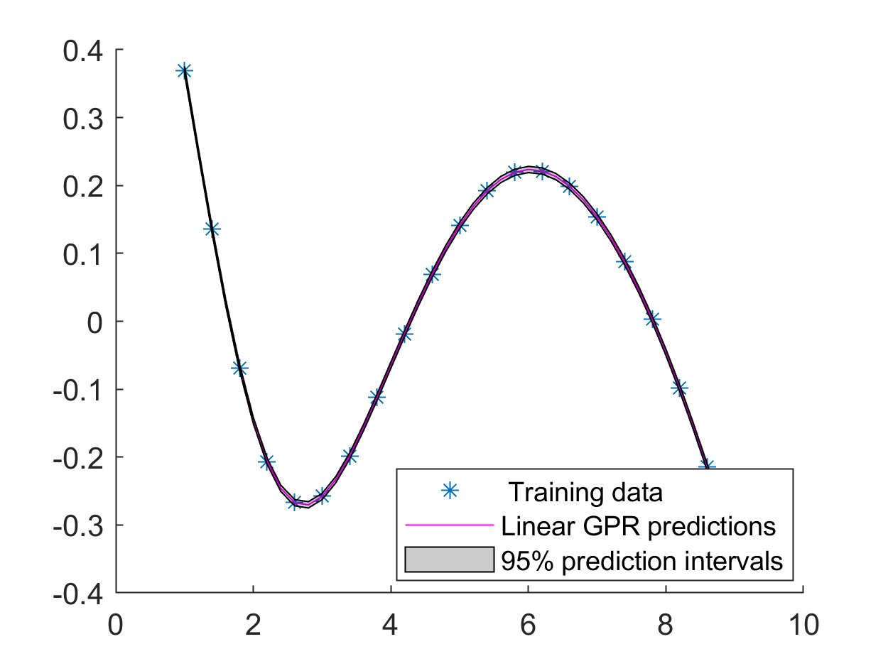
(d) SE Kernel

Figure 19: GPR corresponding to 4th coefficient of the reduced 1st eigenvector of EVP (6) using different kernels.

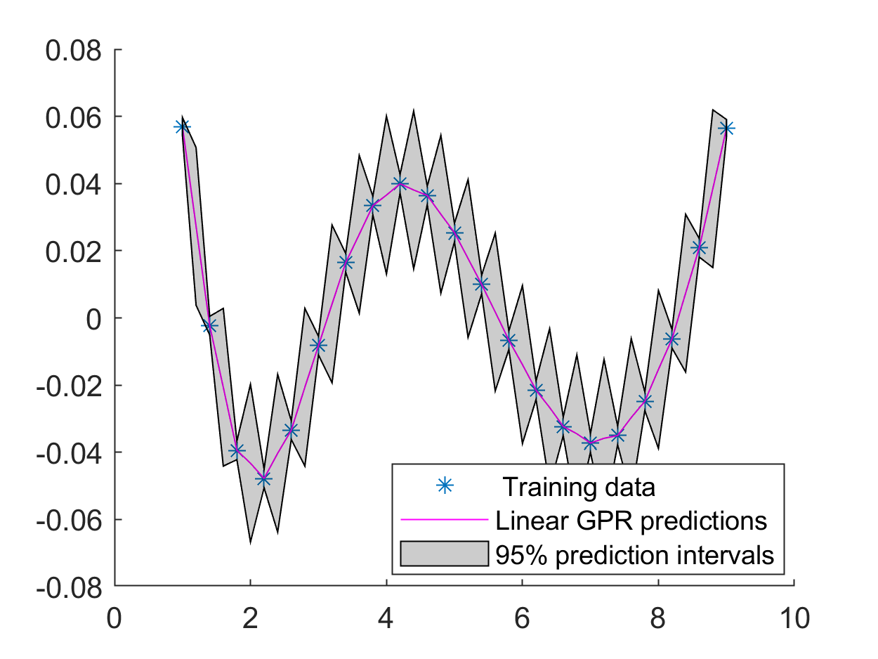
(a) Exp Kernel

(b) Matern 3/2 Kernel

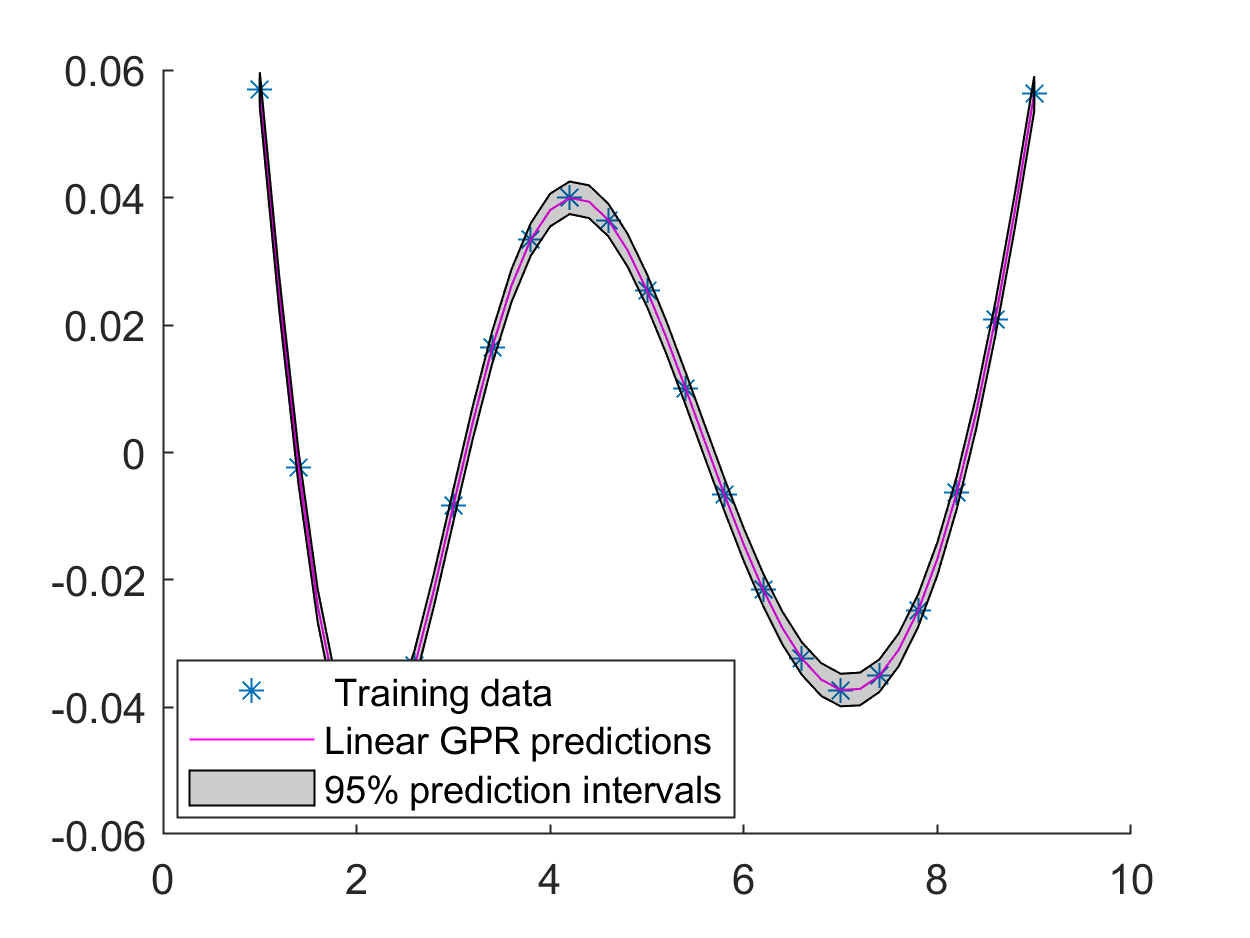
(c) Matern 5/2 Kernel

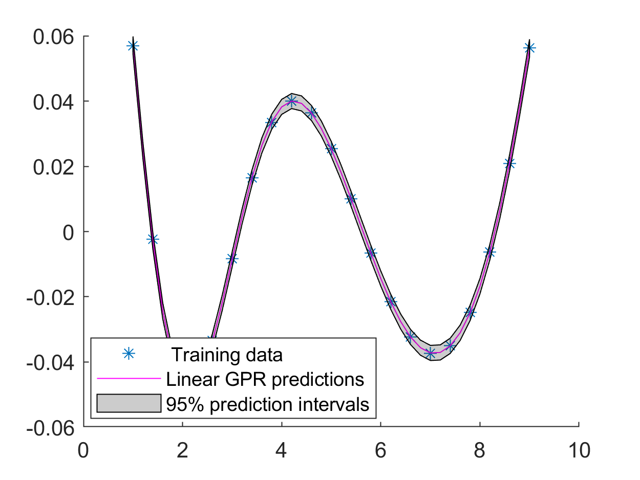
(d) SE Kernel

Figure 20: GPR corresponding to 5th coefficient of the reduced 1st eigenvector of EVP (6) using different kernels.

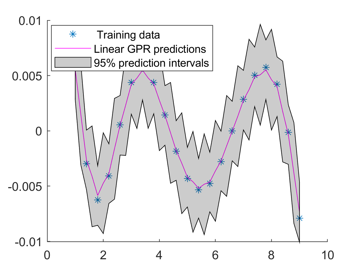
(a) Exp Kernel

(b) Matern 3/2 Kernel

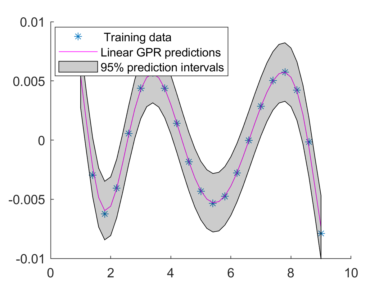
(c) Matern 5/2 Kernel

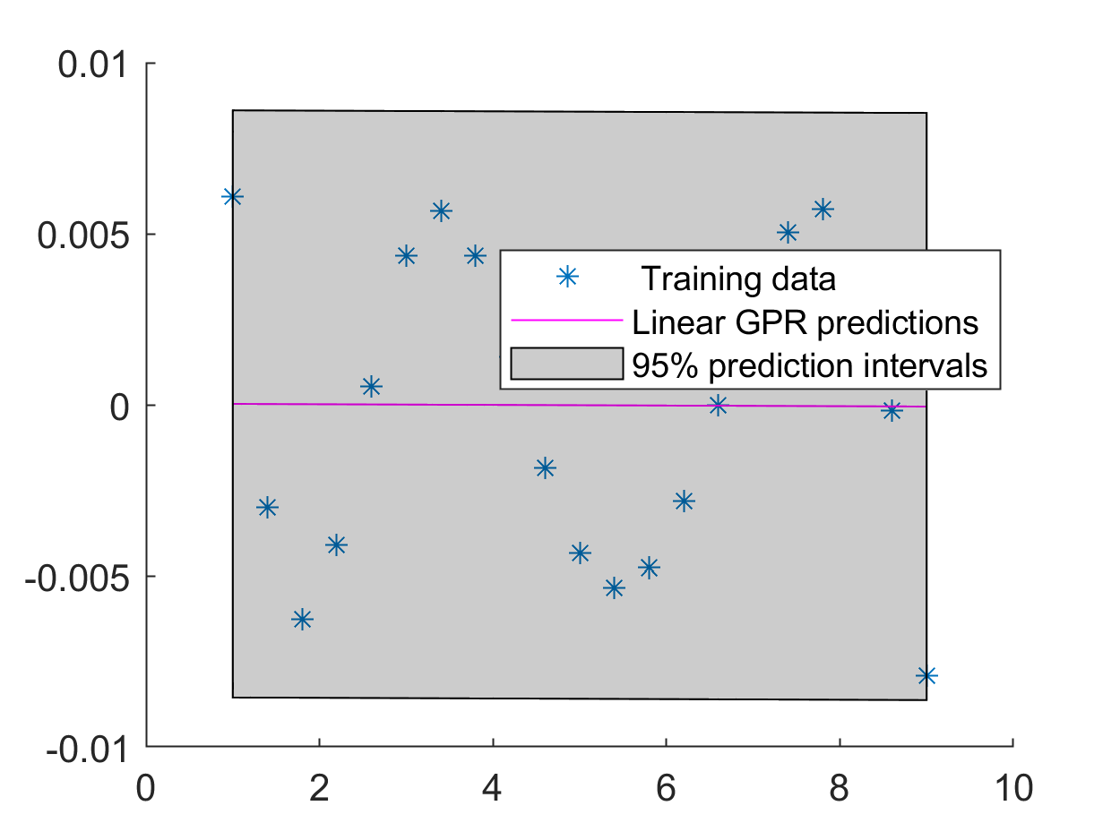
(d) SE Kernel

Figure 21: GPR corresponding to sixth coefficient of the reduced 1st eigenvector of EVP (6) using different kernels.

(a) Exp Kernel

(b) Matern 3/2 Kernel

(c) Err Matrn 5/2 Kernel

(d) SE Kernel

Figure 22: Error between the FEM and GPR-based first eigenvectors of EVP (6) using different kernels at $\mu=1.6$.

(a) Exp Kernel

(b) Matern 3/2 Kernel

(c) Err Matrn 5/2 Kernel

(d) SE Kernel

Figure 23: Error between the FEM and GPR-based second eigenvectors of EVP (6) using different kernels at $\mu=1.6$.

Example 3

Let us consider the following eigenvalue problem

$$\left\{\begin{aligned} &-\Delta u(\mu)=\lambda(\mu)e^{-\mu(x^{2}+y^{2})}u(\mu)&&\text{in }\Omega=(0,1)^{2}\\ &u(\mu)=0&&\text{on }\partial\Omega,\end{aligned}\right.$$ (7)

where the parameter $\mu$ belongs to the set $\mathcal{P}=[1,8]$. The parameters used for training are $\mu_{tr}=1:0.4:8$ and test points are $\mu_{tr}=1:0.2:8$. Note that this EVP is non-affine parameter dependent. The first five eigenvalues of this problem are shown in Figure 24.

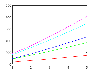
Figure 24: First four eigenvalues of the EVP (7).

In Figure 25, we have shown the GPR with the interval of confidence for the first eigenvalues of the EVP (7) using four different covariance functions. The first and second eigenvalues are compared at the four test points $\mu=1.6,3.6,5.6,7.6$ and the corresponding relative error is also reported in Table 6 and Table 7 respectively. Relative root mean squared error(RRMSE) between the FEM solution and GPR-based data-driven models are reported in the last column of the table using the test data set $\mu_{tst}=1:0.2:8$. Although all four GPR models are giving comparable results, the models with Matern kernels are better than the other two. In this case, we have five reduced coefficients corresponding to the first eigenvectors. In Figure 26-Figure 30, we have plotted the GPR for the coefficients corresponding to the first eigenvector. In Figure 31, we have shown the error between the first eigenvector obtained by FEM and the corresponding eigenvectors using GPR with different kernels at $\mu=7.6$. The errors are of order $10^{-4}$.

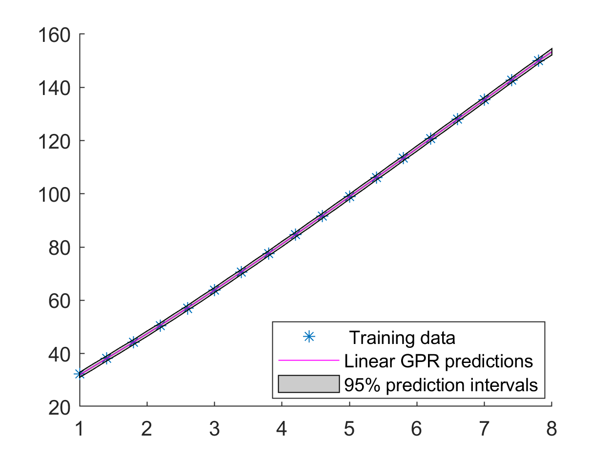
(a) Exp Kernel

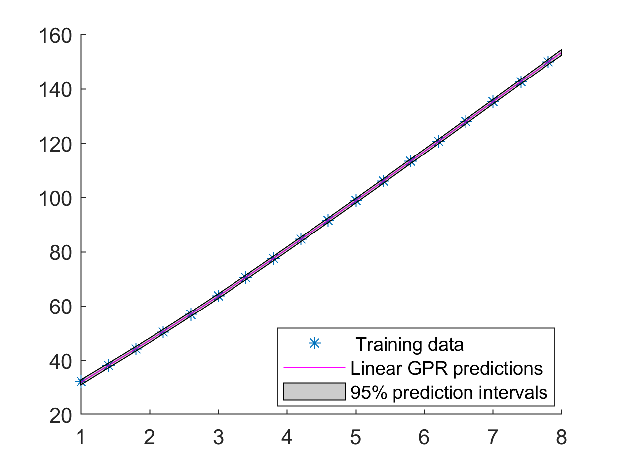
(b) Matern 3/2 Kernel

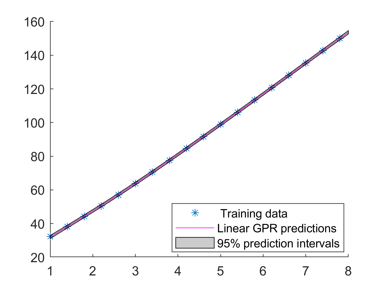
(c) Matern 5/2 Kernel

(d) Squared Exponential Kernel

Figure 25: GPR corresponding to 1st eigenvalues of EVP 7 using different kernels.

Cov	Method	$\mu=1.6$	$\mu=3.6$	$\mu=5.6$	$\mu=7.6$	RRMSE
	FEM	41.14477131	74.09209731	109.74674812	146.40689496
Exp	GPR	41.22202687	74.16102880	109.77496319	146.30273559	$2.0\times 10^{-4}$
	Rel. Err	$1.9\times 10^{-3}$	$9.3\times 10^{-4}$	$2.5\times 10^{-4}$	$7.1\times 10^{-4}$
Matern 3/2	GPR	41.27778797	74.09210663	109.75247219	146.35196960	$1.5\times 10^{-4}$
	Rel. Err	$3.2\times 10^{-3}$	$1.2\times 10^{-5}$	$5.2\times 10^{-5}$	$3.7\times 10^{-4}$
Matern 5/2	GPR	41.28116501	74.06563189	109.75515782	146.35180876	$1.6\times 10^{-4}$
	Rel. Err	$3.3\times 10^{-3}$	$3.5\times 10^{-4}$	$7.6\times 10^{-5}$	$3.7\times 10^{-4}$
SE	GPR	41.26965874	74.03982795	109.76292084	146.32569948	$2.2\times 10^{-4}$
	Rel. Err	$3.0\times 10^{-3}$	$7.0\times 10^{-4}$	$1.4\times 10^{-4}$	$5.5\times 10^{-4}$

Table 6: Comparision of 1st eigenvalues of (7) using GPR model with different covariance functions.

Cov	Method	$\mu=1.6$	$\mu=3.6$	$\mu=5.6$	$\mu=7.6$	RRMSE
	FEM	102.76210685	181.82493491	267.98372293	357.03678494
Exp	GPR	102.90773066	181.99507553	268.05740137	356.78419534	$1.9\times 10^{-4}$
	Rel. Err	$1.4\times 10^{-3}$	$9.3\times 10^{-4}$	$2.7\times 10^{-4}$	$7.0\times 10^{-4}$
Matern 3/2	GPR	103.02713256	181.83137970	267.99629871	356.90555947	$1.4\times 10^{-4}$
	Rel. Err	$2.6\times 10^{-3}$	$3.5\times 10^{-5}$	$4.6\times 10^{-5}$	$3.6\times 10^{-4}$
Matern 5/2	GPR	103.02304342	181.77268604	268.00132001	356.90495184	$1.4\times 10^{-4}$
	Rel. Err	$2.5\times 10^{-3}$	$2.8\times 10^{-4}$	$6.5\times 10^{-5}$	$3.6\times 10^{-4}$
SE	GPR	102.98414556	181.73435363	268.00598508	356.85275445	$2.0\times 10^{-4}$
	Rel. Err	$2.2\times 10^{-3}$	$4.9\times 10^{-4}$	$8.3\times 10^{-5}$	$5.1\times 10^{-4}$

Table 7: Comparison of 2nd eigenvalues of (7) using GPR model with different covariance function.

(a) Exp Kernel

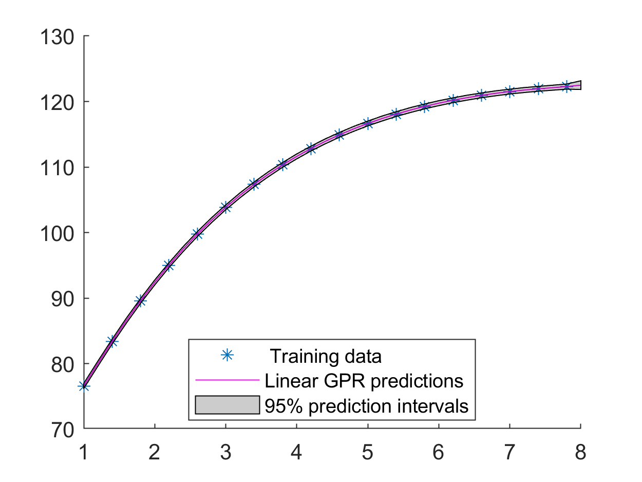
(b) Matern 3/2 Kernel

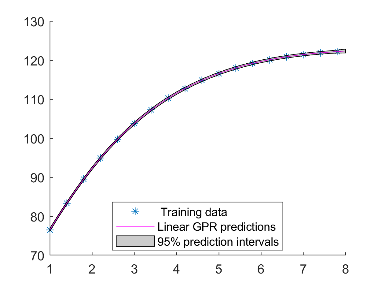
(c) Matern 5/2 Kernel

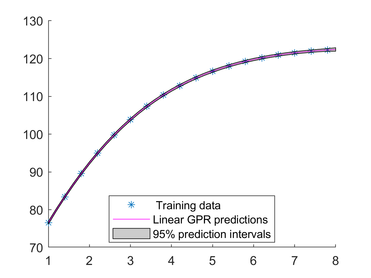
(d) Squared Exponential Kernel

Figure 26: GPR corresponding to 1st coefficient of the Reduced 1st eigenvector of EVP 7 using different kernels.

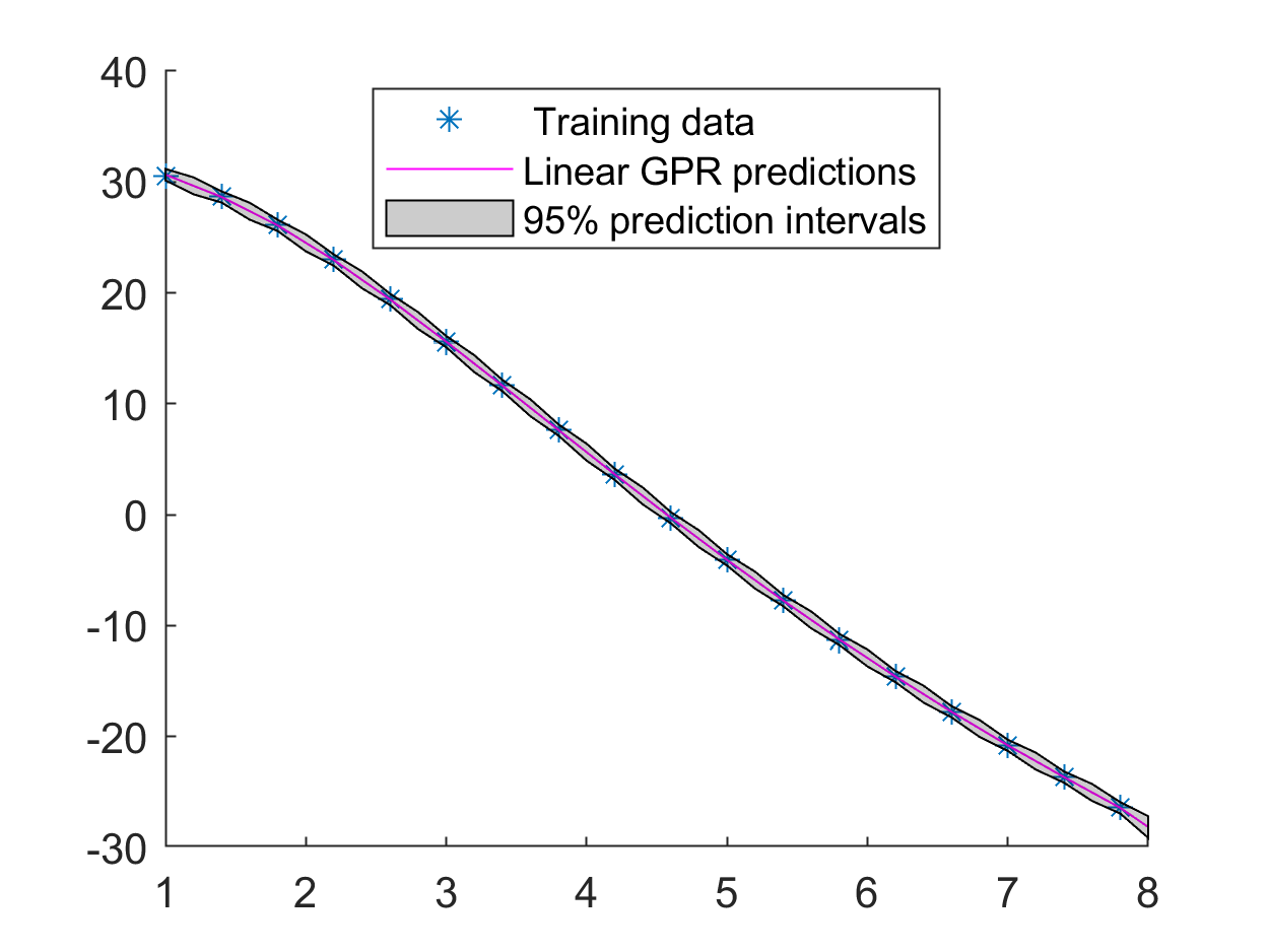
(a) Exp Kernel

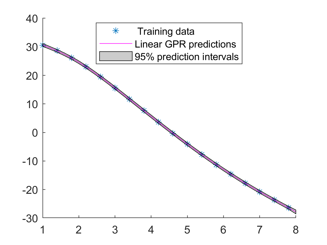
(b) Matern 3/2 Kernel

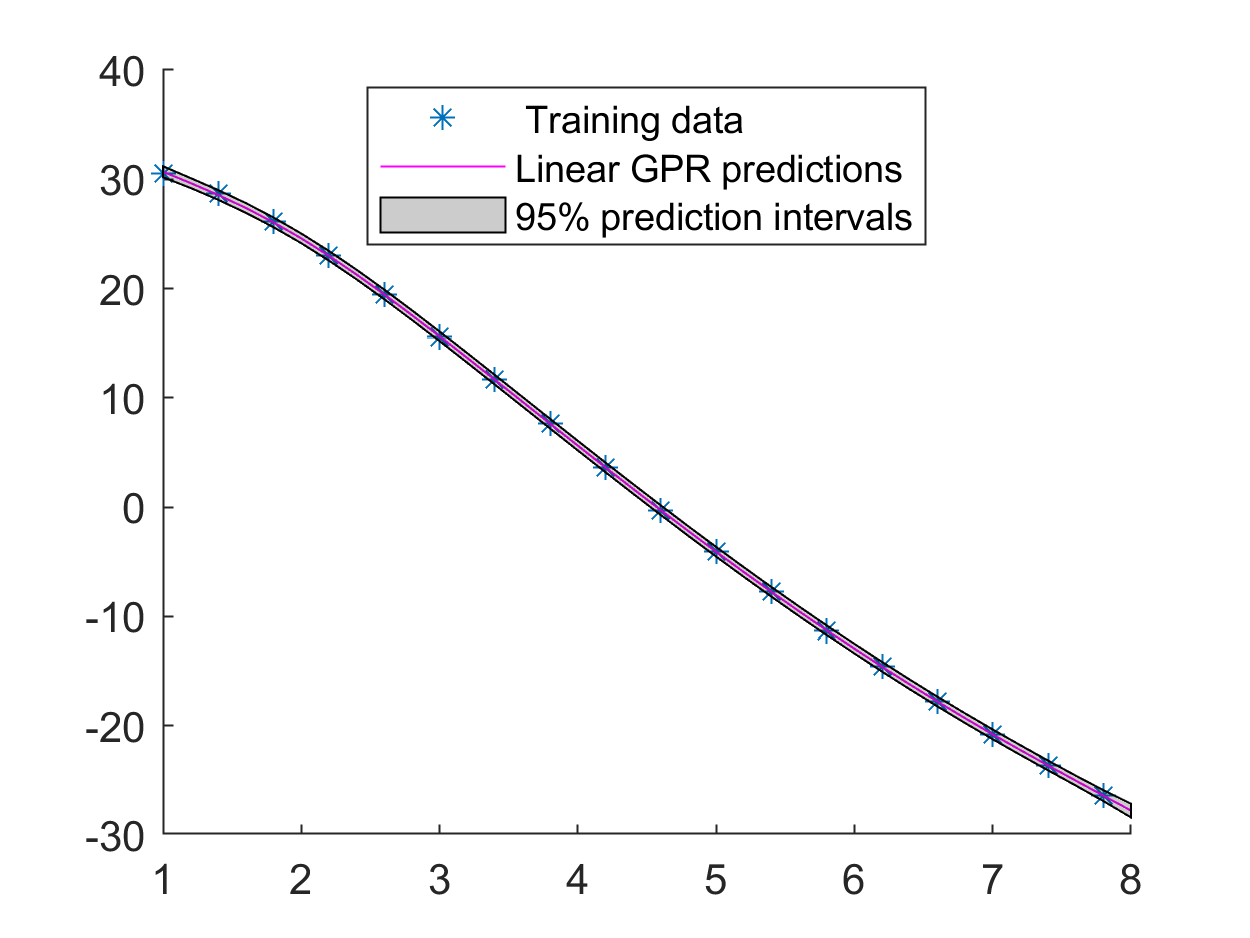
(c) Matern 5/2 Kernel

(d) Squared Exponential Kernel

Figure 27: GPR corresponding to 2nd coefficient of the Reduced 1st eigenvector of EVP 7 using different kernels.

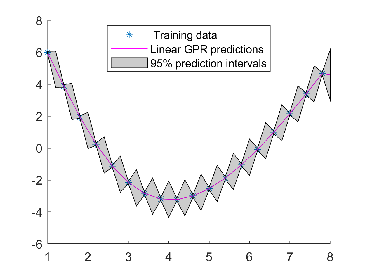
(a) Exp Kernel

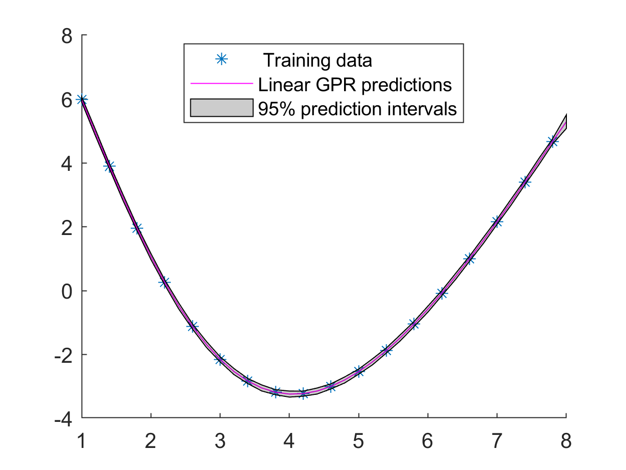
(b) Matern 3/2 Kernel

(c) Matern 5/2 Kernel

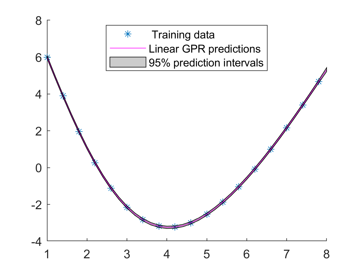
(d) Squared Exponential Kernel

Figure 28: GPR corresponding to 3rd coefficient of the Reduced 1st eigenvector of EVP 7 using different kernels.

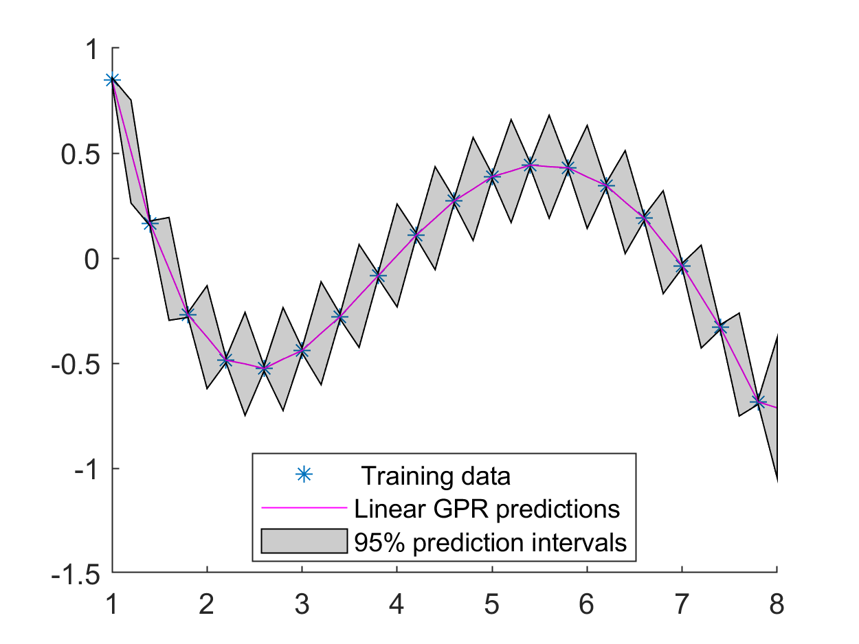
(a) Exp Kernel

(b) Matern 3/2 Kernel

(c) Matern 5/2 Kernel

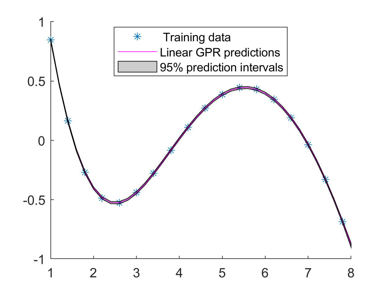
(d) Squared Exponential Kernel

Figure 29: GPR corresponding to 4th coefficient of the Reduced 1st eigenvector of EVP 7 using different kernels.

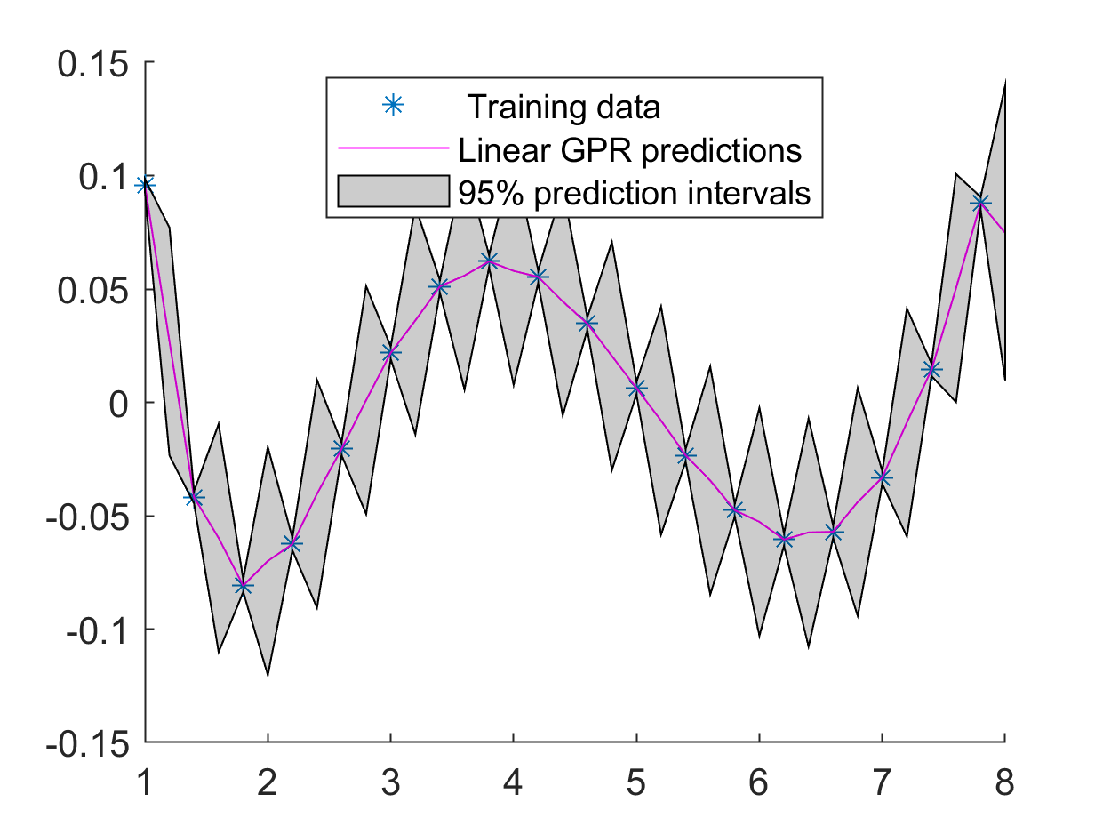
(a) Exp Kernel

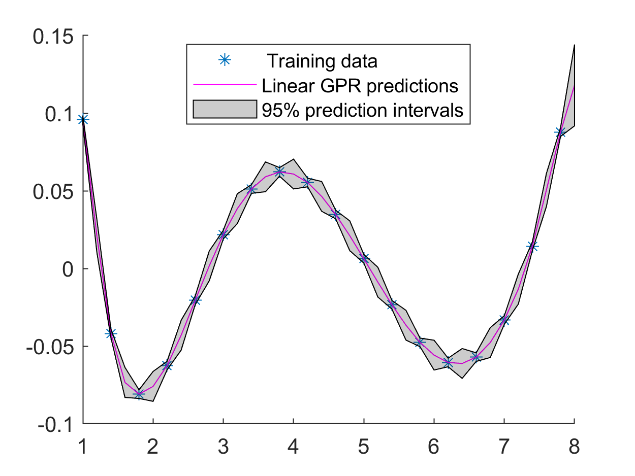
(b) Matern 3/2 Kernel

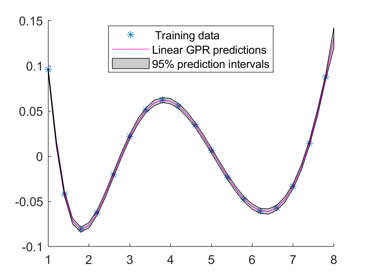
(c) Matern 5/2 Kernel

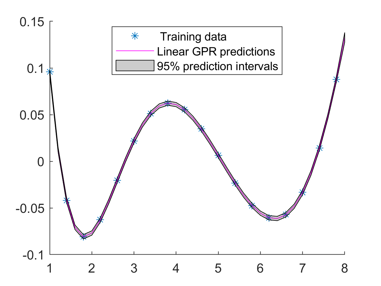
(d) Squared Exponential Kernel

Figure 30: GPR corresponding to 5th coefficient of the Reduced 1st eigenvector of EVP 7 using different kernels.

(a) Exp Kernel

(b) Matern 3/2 Kernel

(c) Err Matrn 5/2 Kernel

(d) SE Kernel

Figure 31: Error between the FEM and GPR-based first eigenvectors of the Nonaffine example using different kernels at $\mu=7.6$.

Example 4

Consider the nonlinear eigenvalue problem of the following form: given any $\mu\in\mathcal{P}$ find $\lambda(\mu)\in\mathbb{R}$ and $u(\mu)\in V$ with $u(\mu)\neq 0$ satisfying

$$\left\{\begin{aligned} &a(u(\mu),v)+\mu^{2}\int_{\Omega}g(u(\mu))v=\lambda(\mu)m(u(\mu),v),\quad\forall v\in V\\ &(u(\mu),u(\mu))=1,\end{aligned}\right.$$ (8)

where $g$ is a nonlinear function. For our numerical tests we consider $\Omega=(0,1)\subset\mathbb{R}$ and the parameter space is $\mathcal{P}=[1,9]$. For given $\mu\in\mathcal{P}$, we solve problem (8) for the following particular choice of data:

$$a(w,v)=\int_{\Omega}\frac{dw}{dx}\frac{dv}{dx},\quad m(w,v)=\int_{\Omega}wvdx,\quad g(w)=|w|^{7/3}w.$$

The parameters used for training are $\mu_{tr}=1:0.4:9$ and test points are $\mu_{tst}=1:0.2:9$.

In Figure 32, we have shown the GPR with the 95 percent interval of confidence for the first eigenvalues of the EVP (8) using four different covariance functions. The first eigenvalues are compared at the four test points $\mu=1.6,3.6,5.6,7.6$ and the relative error between the FEM solution and GPR-based data-driven models are reported in Table 8. Also, the RRMSE is reported for each GPR-based model using the test set $\mu_{tst}=1:0.2:9$. The RRMSE for all four models is almost the same. In this case, we have four reduced coefficients corresponding to the first eigenvectors. In Figure 33-Figure 36, we have plotted the GPR for the coefficients corresponding to the first eigenvector.

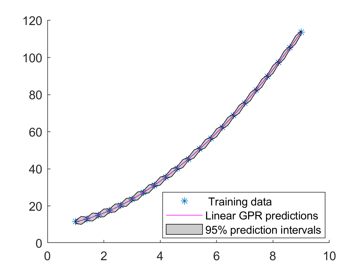
(a) Exp Kernel

(b) Matern 3/2 Kernel

(c) Matern 5/2 Kernel

(d) Squared Exponential Kernel

Figure 32: GPR corresponding to 1st eigenvalues of EVP (8) using different kernels.

Cov	Method	$\mu=1.6$	$\mu=3.6$	$\mu=5.6$	$\mu=7.6$	RRMSE
	FEM	13.93889958	29.15002548	53.47689717	86.02771734
Exp	GPR	14.00702594	29.20715155	53.52966738	86.07774624	$1.1\times 10^{-4}$
	Rel Err	$4.9\times 10^{-3}$	$2.0\times 10^{-3}$	$9.8\times 10^{-4}$	$5.8\times 10^{-4}$
Ma 3/2	GPR	14.02144190	29.14905543	53.47706009	86.02990429	$1.0\times 10^{-4}$
	Rel Err	$5.9\times 10^{-3}$	$3.3\times 10^{-5}$	$3.0\times 10^{-6}$	$2.5\times 10^{-5}$
Ma 5/2	GPR	14.01570568	29.12438823	53.47471356	86.05388349	$1.0\times 10^{-4}$
	Rel Err	$5.5\times 10^{-3}$	$8.7\times 10^{-4}$	$4.0\times 10^{-5}$	$3.0\times 10^{-4}$
SE	GPR	14.00127136	29.12378839	53.46057325	86.07083648	$1.2\times 10^{-4}$
	Rel Err	$4.5\times 10^{-3}$	$9.0\times 10^{-4}$	$3.0\times 10^{-4}$	$5.0\times 10^{-4}$

Table 8: Comparison of 1st eigenvalues using of EVP (8) using GPR model with different covariance functions.

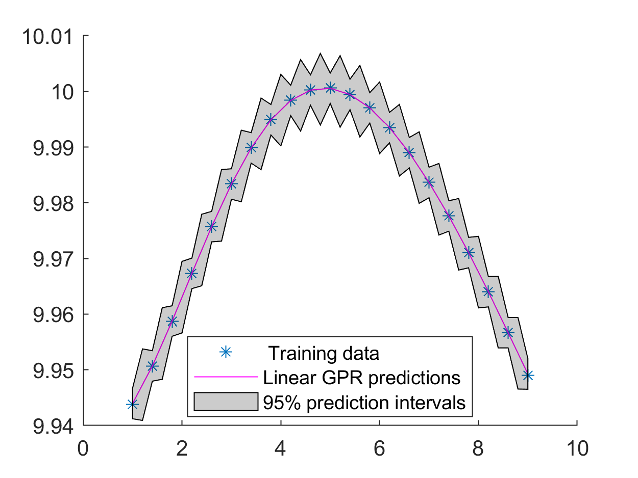
(a) Exp Kernel

(b) Matern 3/2 Kernel

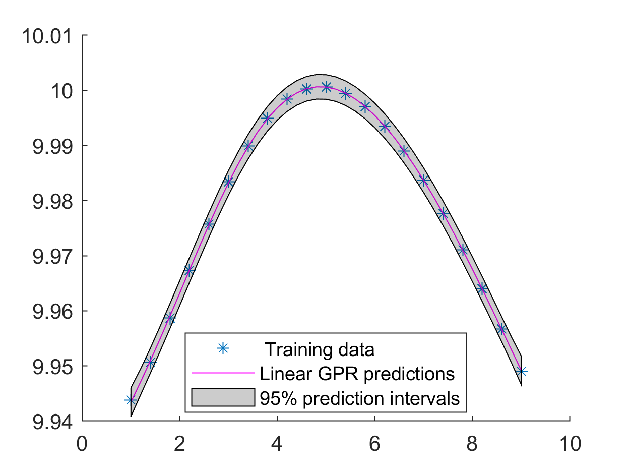
(c) Matern 5/2 Kernel

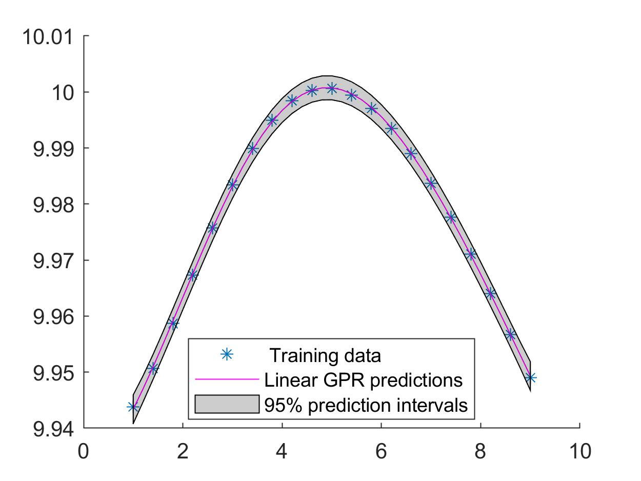
(d) Squared Exponential Kernel

Figure 33: GPR corresponding to 1st coefficient of the Reduced 1st eigenvector of EVP 8 using different kernels.

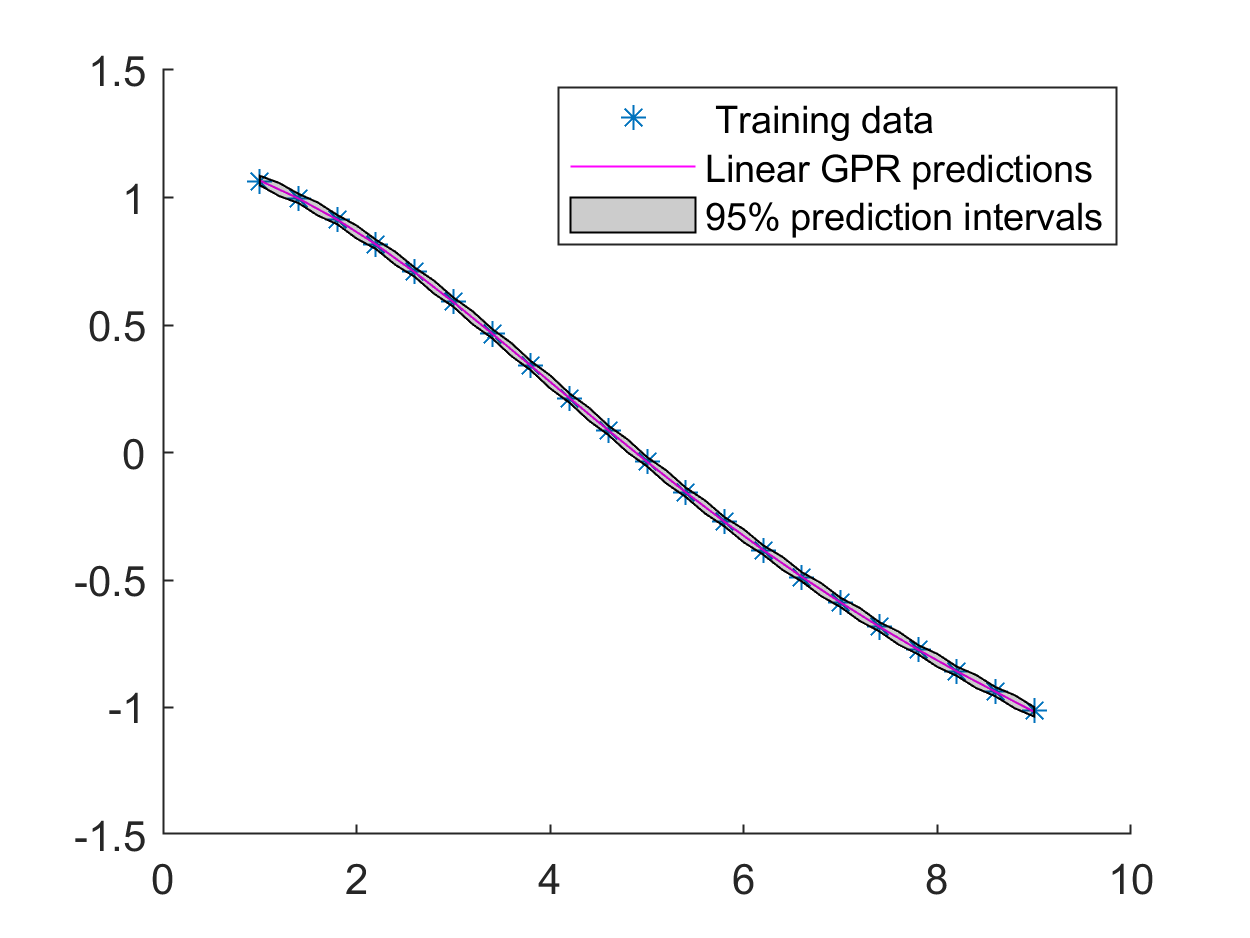
(a) Exp Kernel

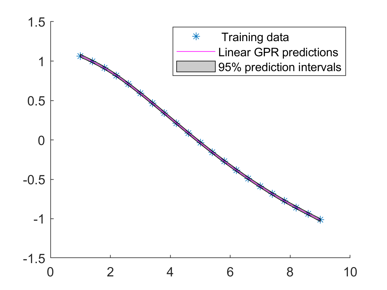
(b) Matern 3/2 Kernel

(c) Matern 5/2 Kernel

(d) Squared Exponential Kernel

Figure 34: GPR corresponding to 2nd coefficient of the Reduced 1st eigenvector of EVP 8 using different kernels.

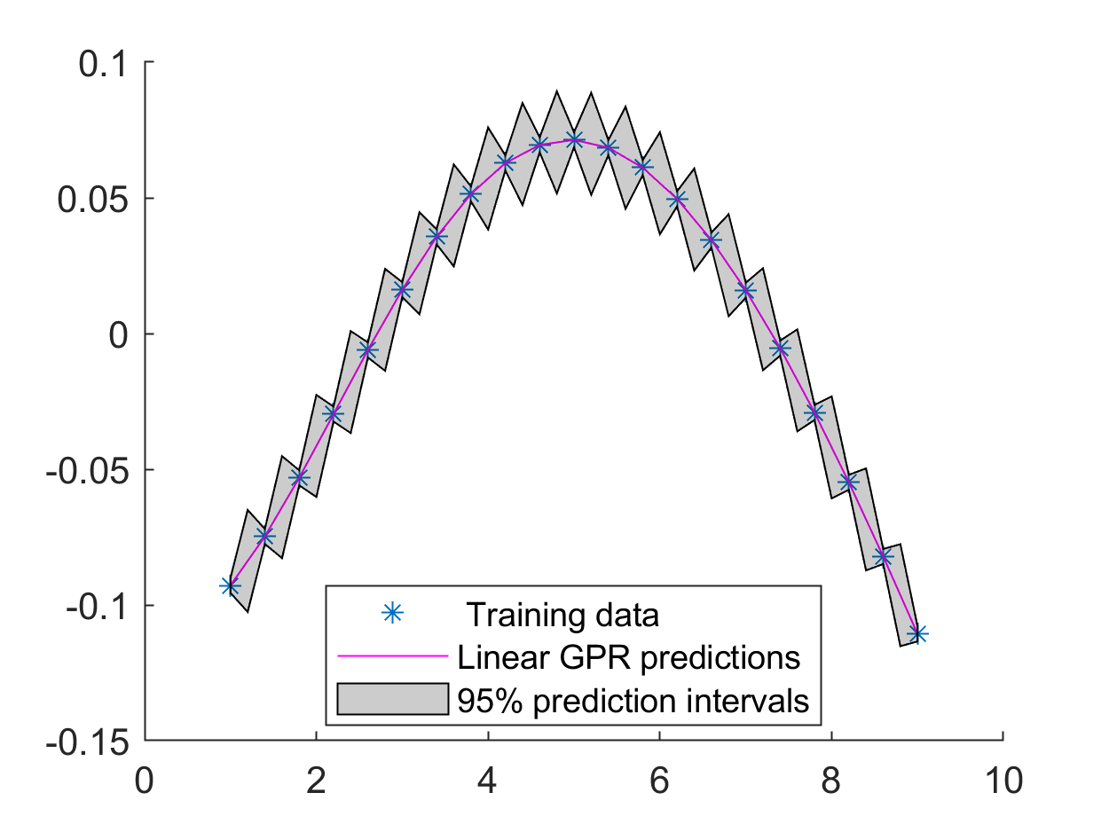
(a) Exp Kernel

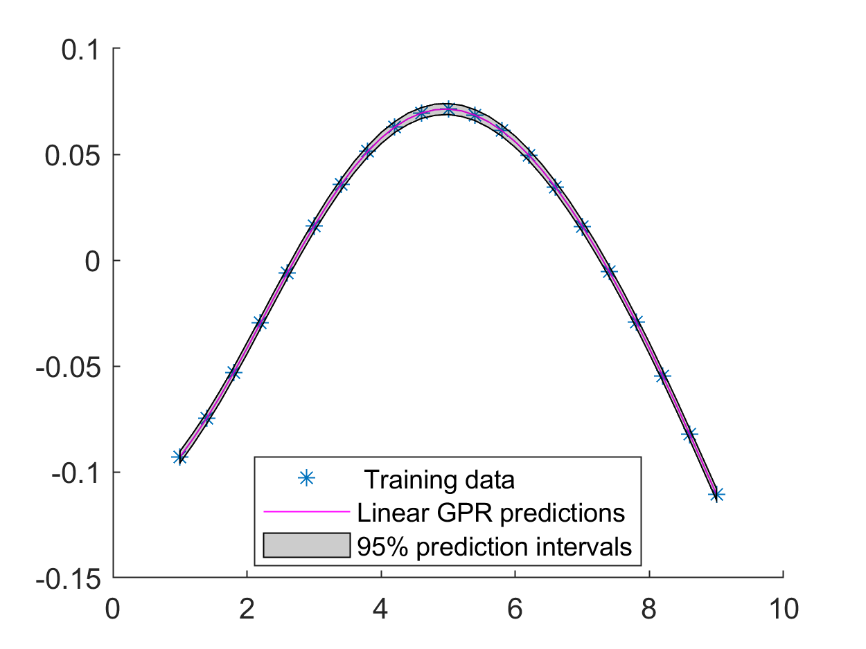
(b) Matern 3/2 Kernel

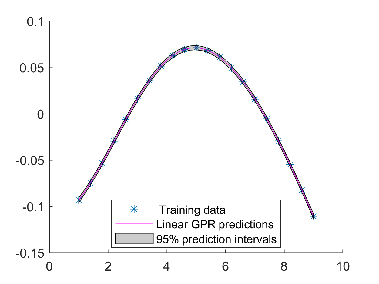
(c) Matern 5/2 Kernel

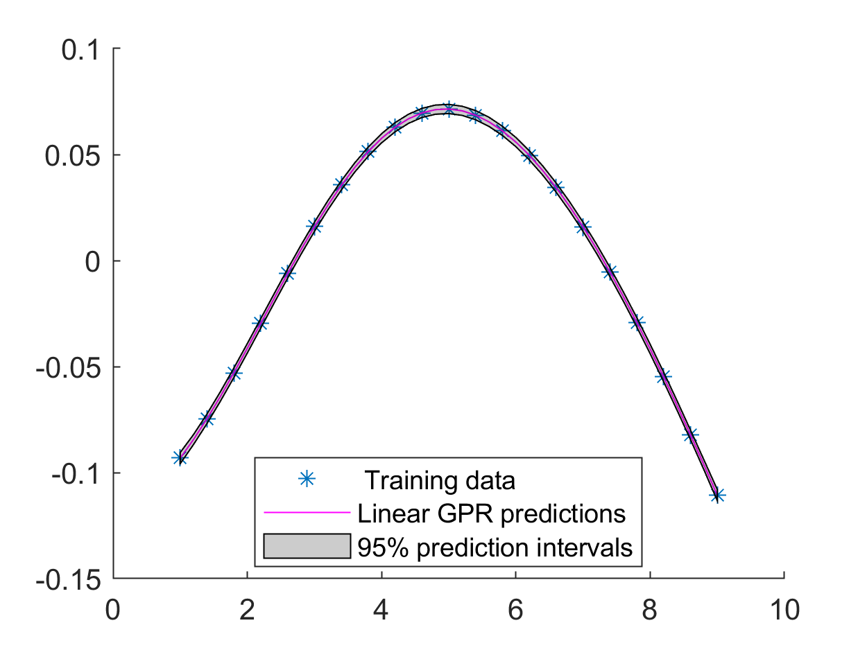
(d) Squared Exponential Kernel

Figure 35: GPR corresponding to 3rd coefficient of the Reduced 1st eigenvector of EVP 8 using different kernels.

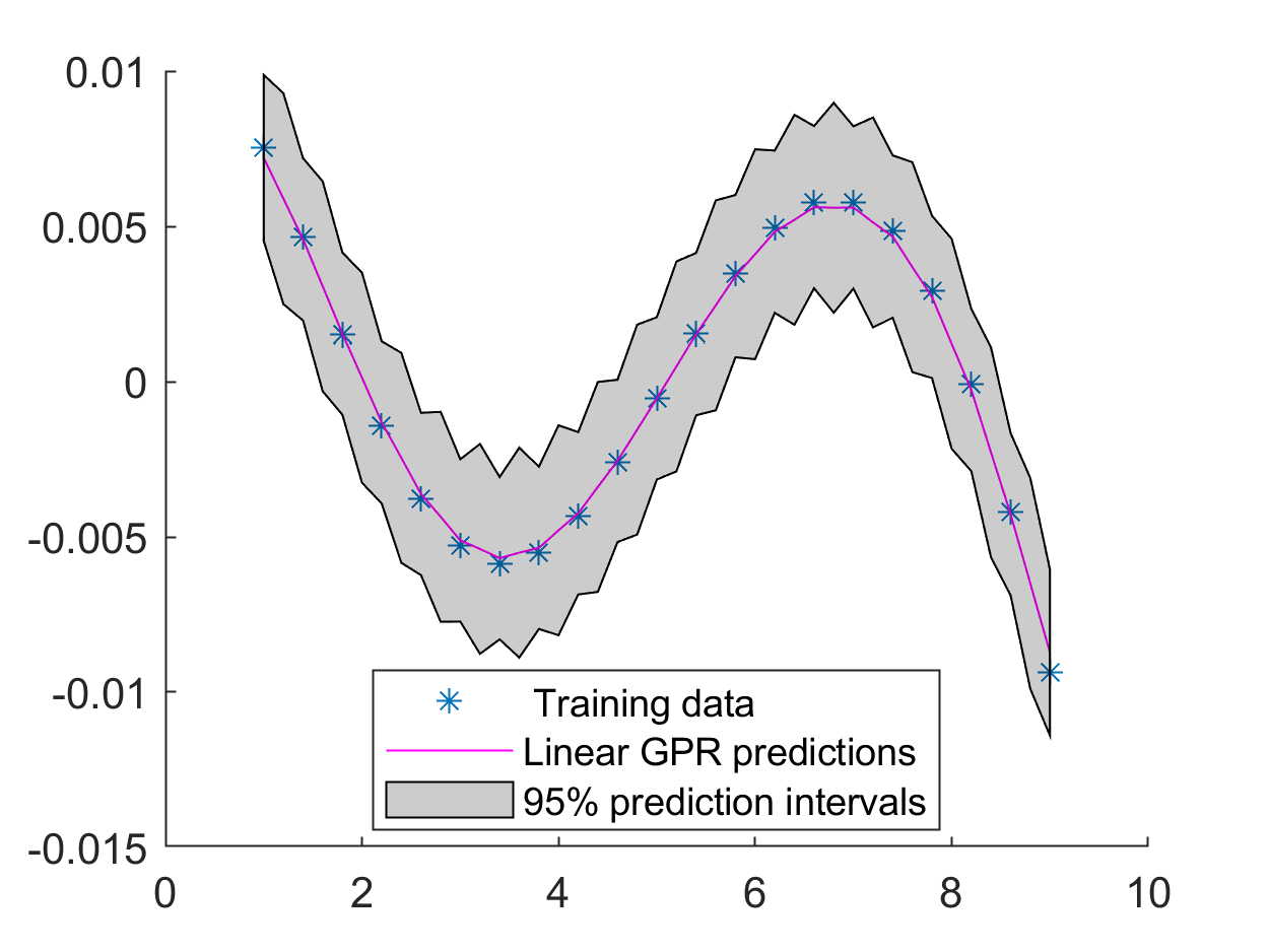
(a) Exp Kernel

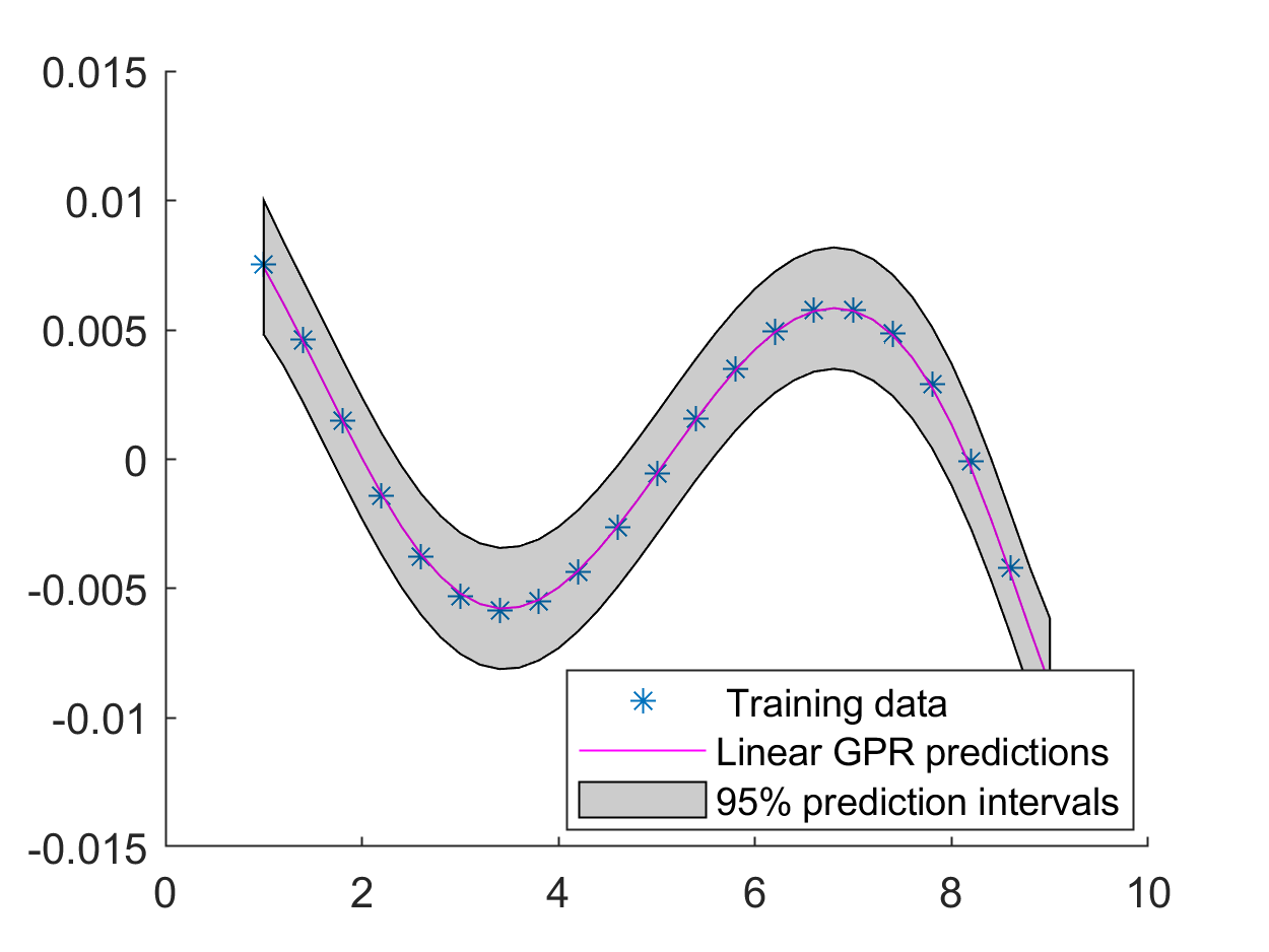
(b) Matern 3/2 Kernel

(c) Matern 5/2 Kernel

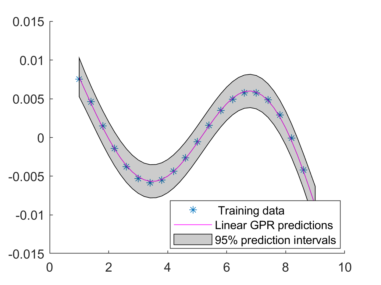
(d) Squared Exponential Kernel

Figure 36: GPR corresponding to 4th coefficient of the Reduced 1st eigenvector of EVP 8 using different kernels.

Example 5

Let us consider the eigenvalue problem

$$\left\{\begin{array}[]{ll}-\operatorname{div}(A(\boldsymbol{\mu})\nabla u(\boldsymbol{\mu}))=\lambda(\boldsymbol{\mu})u(\boldsymbol{\mu})&\textrm{ in }\Omega=(0,1)^{2}\\ u(\boldsymbol{\mu})=0&\textrm{ on }\partial\Omega\end{array}\right.$$ (9)

where the diffusion $A(\boldsymbol{\mu})\in\mathbb{R}^{2\times 2}$ is given by the matrix

$$A(\boldsymbol{\mu})=\begin{pmatrix}\frac{1}{\mu_{1}^{2}}&\frac{0.7}{\mu_{2}}\\ \frac{0.7}{\mu_{2}}&\frac{1}{\mu_{2}^{2}}\end{pmatrix},$$ (10)

with $\boldsymbol{\mu}=(\mu_{1},\mu_{2})\in\mathcal{M}\subset\mathbb{R}^{2}.$ The problem is symmetric and the parameter space $\mathcal{M}$ is chosen in such a way that the matrix is positive definite. The matrix is positive definite for any nonzero value of $\mu_{2}$ and $\mu_{1}\in(-1.42,1.42)\setminus\{0\}$. For the numerical purpose, we choose the parameter space to be $\mathcal{M}=[0.4,1.4]^{2}$. The surface for the first four eigenvalues is shown in Figure 37. Also, to check the intersection we have plotted them separately. We can see that the surface corresponding to the first and second are separate and the 3rd and fourth eigenvalues are intersecting. We have selected 64 uniform sample points, shown in Figure 38(a), from the parameter domain and calculated the solution of the high-fidelity problem at these points and calculate RRMSE we have selected 30 random points from the parameter space and shown the in Figure Figure 38(b).

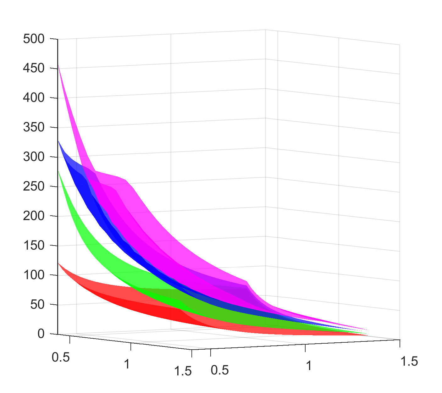
(a) First four eigenvalues

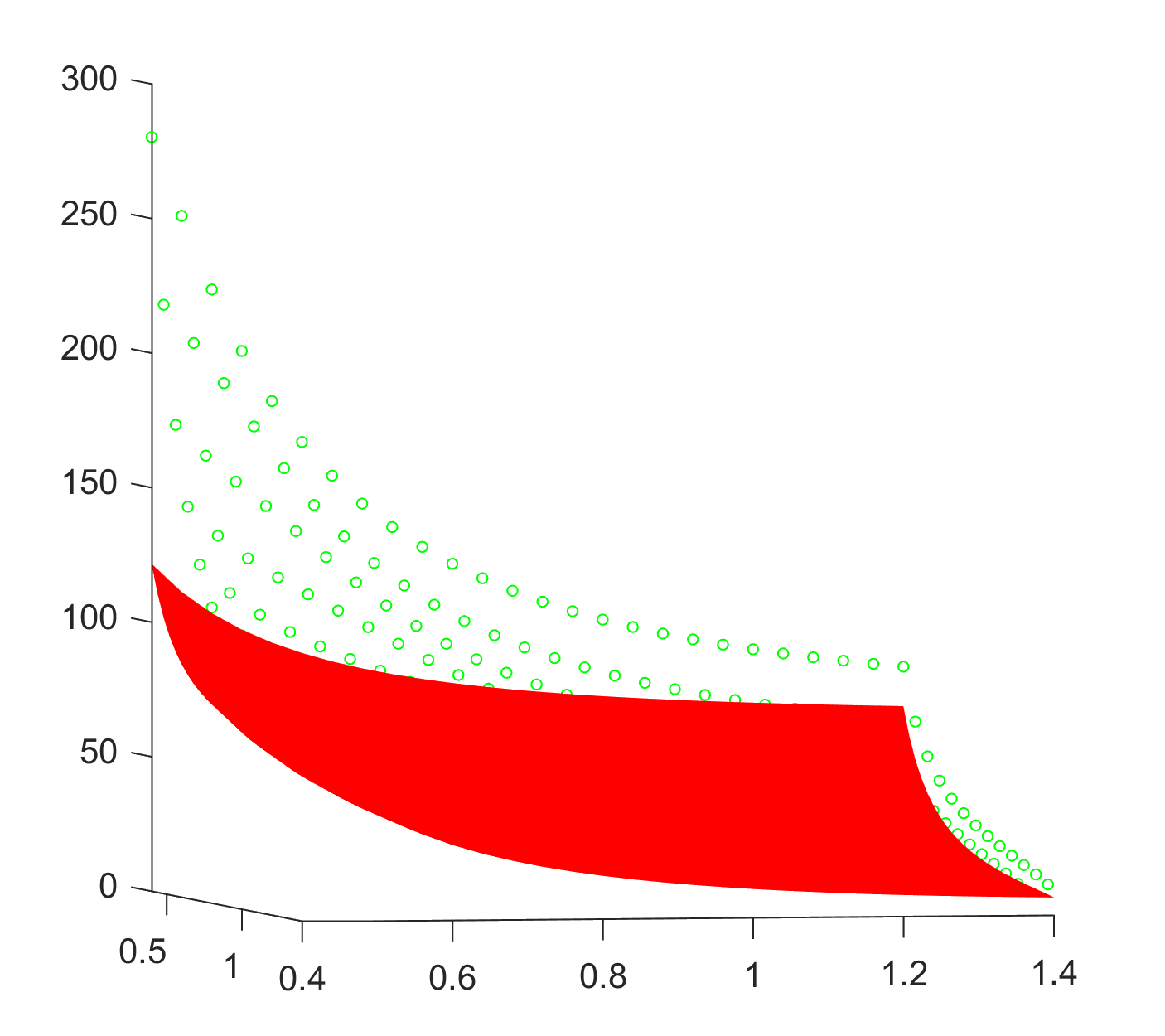
(b) 1st and 2nd eigenvalues

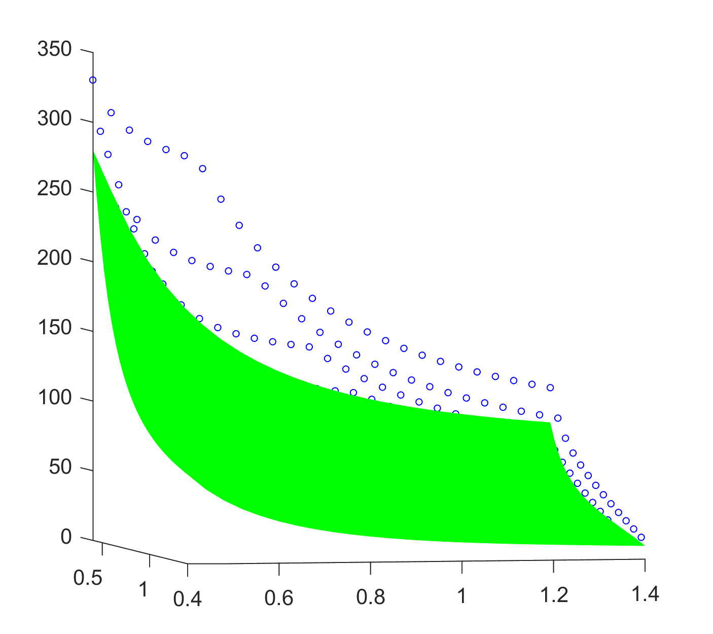
(c) 2nd and 3rd eigenvalues

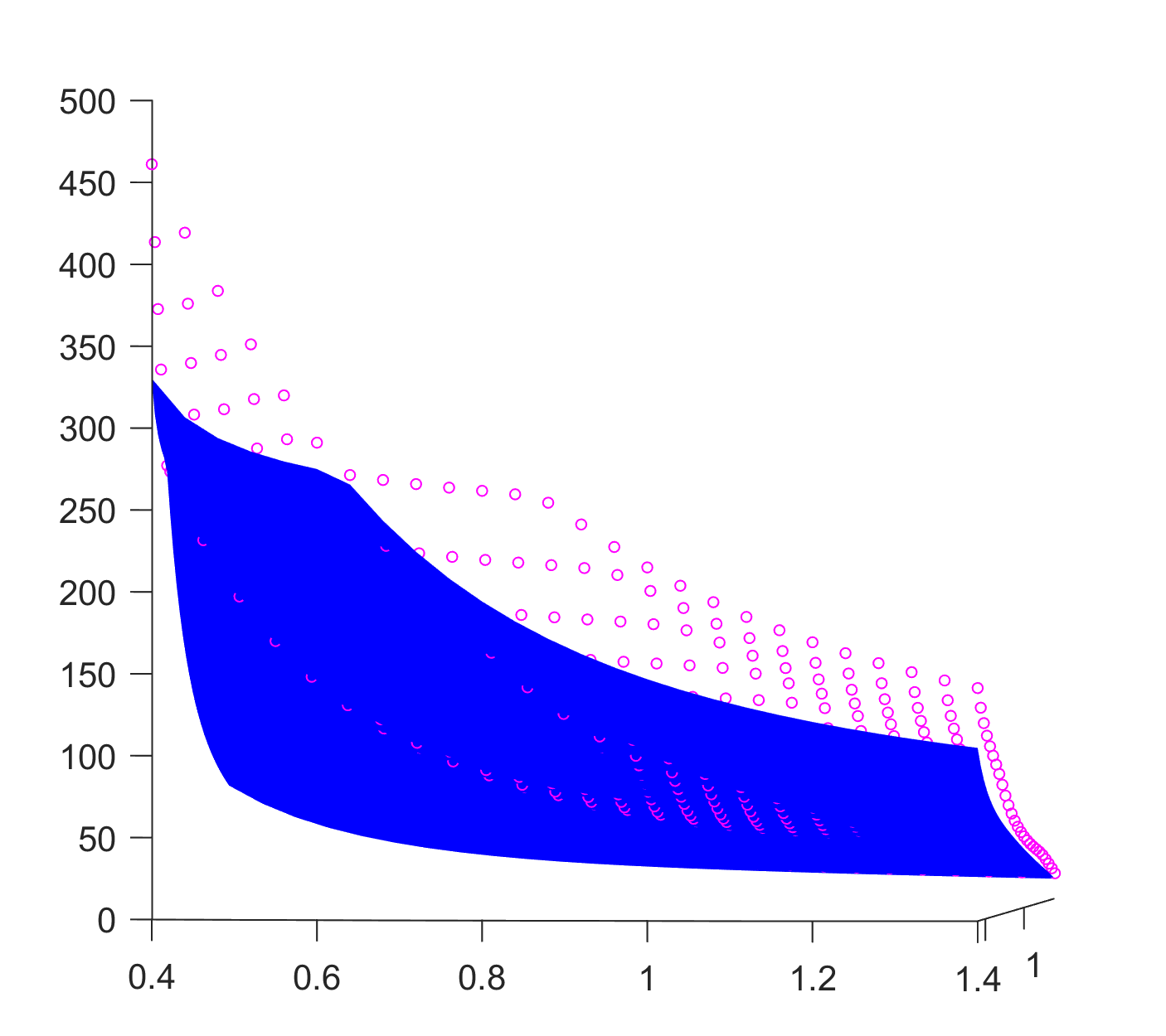
(d) 3rd and 4th eigenvalues

Figure 37: Surface plots eigenvalues of EVP (9).

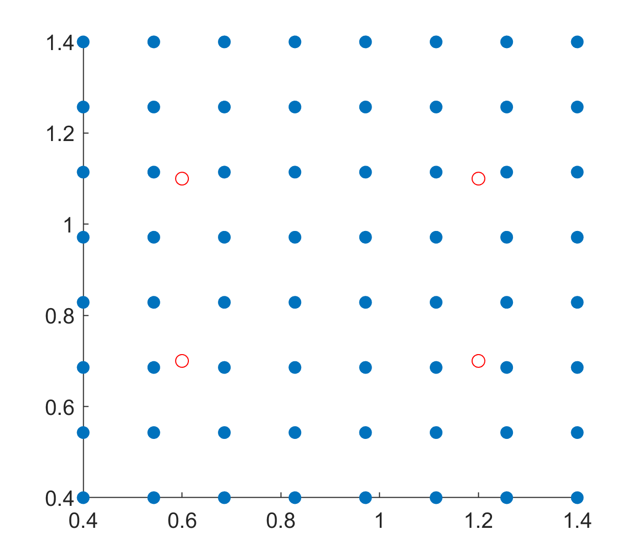
(a) 64 Sample points

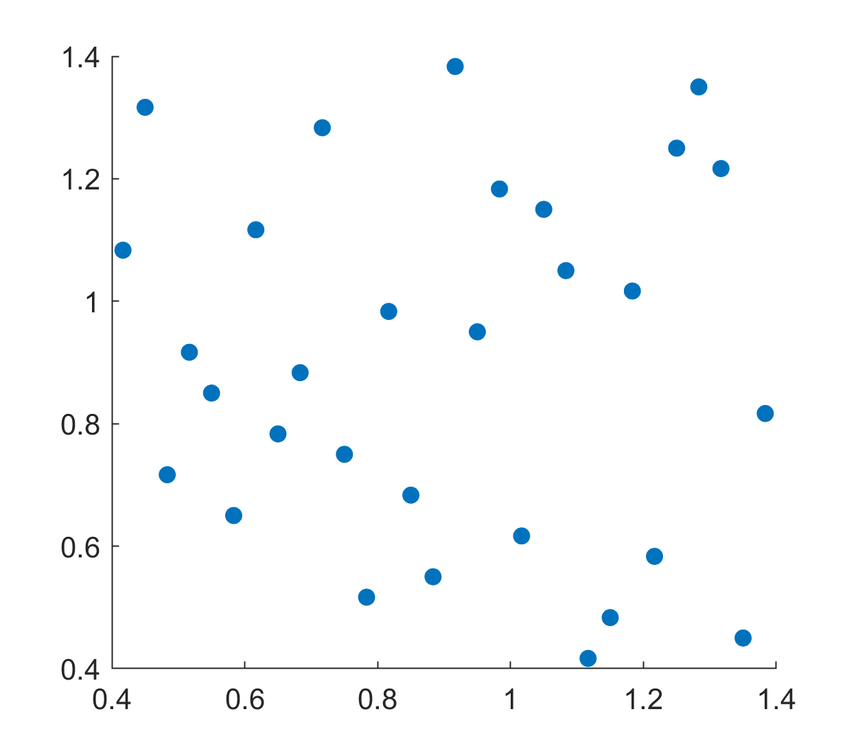
(b) 30 test points

Figure 38: Sampling points and test points for the problem (9).

In Table 9-Table 11 we report the first three eigenvalues of the problem (9) obtained by the GPR method with different kernels at the four test points mentioned in Table. To compare the results at these points we have reported the relative error in each case. To measure the performance of the GPR with different kernels, we have selected 30 random points from the parameter space and calculated the FEM eigenvalues at these points. In the last column of each Table, the RRMSE between the FEM eigenvalues and the GPR-based eigenvalues corresponding to the 30 points are reported in each case. From the RRMSE measure, one can see that the GPR with smooth kernels i.e. squared exponential and Matern 5/2 kernel perform better for the first and second eigenvalues as they are separated but for the case of third eigenvalues, the GPR with less smooth kernels i.e. exponential and Matern 3/2 kernels perform better than the other two.

Cov	Method	$\mu=(0.6,0.7)$	$\mu=(0.6,1.1)$	$\mu=(1.2,0.7)$	$\mu=(1.2,1.1)$	RRMSE
	FEM	45.85197267	34.64251756	23.29248791	12.18646344
Exp	GPR	45.86251454	34.69108864	23.26786125	12.19941643	$5\times 10^{-4}$
	Rel. Err	$2.2\times 10^{-4}$	$1.4\times 10^{-3}$	$1.1\times 10^{-3}$	$1.1\times 10^{-3}$
Matern 3/2	GPR	45.46156207	34.20070168	23.34477917	12.19928855	$4.7\times 10^{-3}$
	Rel. Err	$8.5\times 10^{-3}$	$1.2\times 10^{-2}$	$2.2\times 10^{-3}$	$1.1\times 10^{-3}$
Matern 5/2	GPR	45.59442807	34.40673326	23.27084283	12.19589414	$2.8\times 10^{-3}$
	Rel. Err	$5.6\times 10^{-3}$	$6.8\times 10^{-3}$	$9.2\times 10^{-4}$	$7.7\times 10^{-4}$
SE	GPR	45.49200578	34.33444835	23.04772430	11.99134204	$5\times 10^{-3}$
	Rel. Err	$7.9\times 10^{-3}$	$8.9\times 10^{-3}$	$1.0\times 10^{-2}$	$1.6\times 10^{-2}$

Table 9: Comparison of 1st eigenvalues using GPR model with different covariance functions using 64 uniform training samples.

Cov	Method	$\mu=(0.6,0.7)$	$\mu=(0.6,1.1)$	$\mu=(1.2,0.7)$	$\mu=(1.2,1.1)$	RRMSE
	FEM	96.54372096	56.01413149	32.24518490	20.88096249
Exp	GPR	95.95615765	56.01873345	32.23274693	20.92700367	$2.5\times 10^{-3}$
	Rel. Err	$6.1\times 10^{-3}$	$8.2\times 10^{-5}$	$3.8\times 10^{-4}$	$6\times 10^{-3}$
Matern 3/2	GPR	96.47557137	55.64837627	32.31106319	20.92199772	$1.6\times 10^{-3}$
	Rel. Err	$7.0\times 10^{-4}$	$6.5\times 10^{-3}$	$2.0\times 10^{-3}$	$2.0\times 10^{-3}$
Maatern 5/2	GPR	96.68514232	55.72368588	32.13167982	20.87495342	$1.5\times 10^{-3}$
	Rel. Err	$1.5\times 10^{-3}$	$5.2\times 10^{-3}$	$3.5\times 10^{-3}$	$2.8\times 10^{-4}$
SE	GPR	95.35176666	55.38480542	31.59712873	20.71807138	$6.4\times 10^{-3}$
	Rel. Err	$1.2\times 10^{-2}$	$1.1\times 10^{-2}$	$2.0\times 10^{-2}$	$7.8\times 10^{-3}$

Table 10: Comparison of 2nd eigenvalues using GPR model with different covariance functions using 49 uniform training samples.

Cov	Method	$\mu=(0.6,0.7)$	$\mu=(0.6,1.1)$	$\mu=(1.2,0.7)$	$\mu=(1.2,1.1)$	RRMSE
	FEM	132.64036728	90.30238970	45.43846359	29.99077154
Exp	GPR	135.86386128	90.39244220	45.39209636	30.10292490	$9.5\times 10^{-3}$
	Rel. Err	$2.4\times 10^{-2}$	$9.9\times 10^{-4}$	$1.0\times 10^{-3}$	$3.7\times 10^{-3}$
Maern 3/2	GPR	134.69712089	90.44035171	45.14736699	29.99036891	$6.1\times 10^{-3}$
	Rel. Err	$1.5\times 10^{-2}$	$1.5\times 10^{-3}$	$6.4\times 10^{-3}$	$1.3\times 10^{-5}$
Matern 5/2	GPR	139.73548469	90.29689378	45.07849488	30.15531081	$2.1\times 10^{-2}$
	Rel. Err	$5.3\times 10^{-2}$	$6.0\times 10^{-5}$	$7.9\times 10^{-3}$	$5.5\times 10^{-3}$
SE	GPR	145.85673414	89.79959021	44.87634815	32.70016826	$3.9\times 10^{-2}$
	Rel. Err	$9.9\times 10^{-2}$	$5.6\times 10^{-3}$	$1.2\times 10^{-2}$	$9.0\times 10^{-2}$

Table 11: Comparison of 3rd eigenvalues using GPR model with different covariance functions using 49 uniform training samples.

6 Conclusion

In this paper we have presented some preliminary discussion on how to apply Bayesian methods commonly used in machine learning, to the approximation of parametric PDE eigenvalues problems. After a brief description of GPR, we critically compare GPR and splines for the approximation of data and and functions. We plan to extend this discussion in subsequent investigations.

The main core of our numerical experiments deals with the comparison of different covariance functions in the application of GPR to parametric eigenvalue problems.

A general rule is that the GPR with absolute exponential kernel outperforms if the output data is not smooth, while the GPR with the squared exponential kernel is better if the data is very smooth; otherwise all four GPRs give comparable result. In the applications we have in mind, due to the presence of regions where the parametric dependence is smooth, together with other regions where the parametric dependence is non continuous, it is not immediate to define the best kernel. Further studies and analysis will be performed to design optimal strategy, possibly taking advantage of adaptive procedures and suitable combinations of kernels, and to identify appropriate criteria for the selection of the kernels.

References

- [1] Moataz M. Alghamdi, Daniele Boffi, and Francesca Bonizzoni. A greedy mor method for the tracking of eigensolutions to parametric elliptic pdes, 2022.
- [2] R. Andreev and C. Schwab. Sparse Tensor Approximation of Parametric Eigenvalue Problems, pages 203–241. Springer Berlin Heidelberg, 2012.
- [3] F. Bertrand, D. Boffi, and Halim. Data-driven reduced order modeling for parametric PDE eigenvalue problems using Gaussian process regression. arXiv:2301.08934[math.NA], 2023.
- [4] Christopher M Bishop. Pattern recognition and machine learning. New York : Springer, 2006.
- [5] D. Boffi, A. Halim, and G. Priyadarshi. Reduced basis approximation of parametric eigenvalue problems in presence of clusters and intersections. arXiv:2302.00898 [math.NA], 2023.
- [6] A.G. Buchan, Christopher Pain, and Ionel Navon. A POD reduced order model for eigenvalue problems with application to reactor physics. International Journal for Numerical Methods in Engineering, 95(12):1011–1032, 2013.
- [7] Zexun Chen, Jun Fan, and Kuo Wang. Multivariate gaussian processes: definitions, examples and applications. METRON, jan 2023.
- [8] P Craven and G Wahba. Smoothing noisy data with spline functions. Numerische Mathematik, 31:377–403, 1978.
- [9] David G. T. Denison, Christopher C. Holmes, Bani K. Mallick, and Adrian F.M. Smith. Bayesian Methods for Nonlinear Classification and Regression. Wiley, 2002.
- [10] Peter I. Frazier. A tutorial on bayesian optimization, 2018.
- [11] Fumagalli, I., Manzoni, A., Parolini, N., and Verani, M. Reduced basis approximation and a posteriori error estimates for parametrized elliptic eigenvalue problems. ESAIM: M2AN, 50(6):1857–1885, 2016.
- [12] P. German and J. C. Ragusa. Reduced-order modeling of parameterized multi-group diffusion k-eigenvalue problems. Annals of Nuclear Energy, 134:144–157, 2019.
- [13] P. J. Green and B. W. Silverman. Nonparametric Regression and Generalized Linear Models. Springer, 1994.
- [14] Mengwu Guo and Jan S. Hesthaven. Reduced order modeling for nonlinear structural analysis using gaussian process regression. Computer Methods in Applied Mechanics and Engineering, 341:807–826, 2018.
- [15] H. Hakula, V. Kaarnioja, and M. Laaksonen. Approximate methods for stochastic eigenvalue problems. Applied Mathematics and Computation, 267:664–681, 2015.
- [16] T. Hastie and R. Tibshirani. Generalized additive models. Chemometrics and Intelligent Laboratory Systems, 1(3):297––310, 1986.
- [17] T. Horger, B. Wohlmuth, and T. Dickopf. Simultaneous reduced basis approximation of parameterized elliptic eigenvalue problems. ESAIM: M2AN, 51(2):443–465, 2017.
- [18] Hiroyuki Kano, Hiroyuki Fujioka, and Clyde F. Martin. Optimal smoothing spline with constraints on its derivatives. In 49th IEEE Conference on Decision and Control (CDC), pages 6785–6790, 2010.
- [19] George S. Kimeldorf and Grace Wahba. A correspondence between bayesian estimation on stochastic processes and smoothing by splines. https://doi.org/10.1214/aoms/1177697089, 41:495–502, 4 1970.
- [20] L. Machiels, Y. Maday, I.B. Oliveira, A.T. Patera, and D.V. Rovas. Output bounds for reduced-basis approximations of symmetric positive definite eigenvalue problems. Comptes Rendus de l’Académie des Sciences - Series I - Mathematics, 331(2):153–158, 2000.
- [21] G.S.H. Pau. Reduced-basis method for band structure calculations. Phys. Rev. E, 76:046704, 2007.
- [22] G.S.H. Pau. Reduced basis method for quantum models of crystalline solids. Ph.D. thesis, Massachusetts Institute of Technology, 2008.
- [23] A. Quarteroni, A. Manzoni, and F. Negri. Reduced basis methods for partial differential equations: An introduction. Springer, 2016.
- [24] A. Quarteroni and G. Rozza. Numerical solution of parametrized navier-stokes equations by reduced basis methods. Numerical Methods for Partial Differential Equations, 23(4):923–948, 2007.
- [25] Christopher K. I. Rasmussen, Carl Edward Williams. Gaussian Processes for Machine Learning. The MIT Press, 2005.
- [26] S. Vallaghé, P. Huynh, D.J Knezevic, L. Nguyen, and A.T. Patera. Component-based reduced basis for parametrized symmetric eigenproblems. Advanced Modeling and Simulation in Engineering Sciences, 2(1):1–30, 2015.
- [27] G. Wahba. Spline Models for Observational Data. Siam, 1990.
- [28] B. Wang and T. Chen. Gaussian process regression with multiple response variables. Chemometrics and Intelligent Laboratory Systems, 142:159––165, 2015.