SEOBNRv5PHM: Next generation of accurate and efficient multipolar precessing-spin effective-one-body waveforms for binary black holes

Abstract

Spin precession is one of the key physical effects that could unveil the origin of the compact binaries detected by ground- and space-based gravitational-wave (GW) detectors, and shed light on their possible formation channels. Efficiently and accurately modeling the GW signals emitted by these systems is crucial to extract their properties. Here, we present SEOBNRv5PHM, a multipolar precessing-spin waveform model within the effective-one-body (EOB) formalism for the full signal (i.e. inspiral, merger and ringdown) of binary black holes (BBHs). In the non-precessing limit, the model reduces to SEOBNRv5HM, which is calibrated to $442$ numerical-relativity (NR) simulations, $13$ waveforms from BH perturbation theory, and non-spinning energy flux from second-order gravitational self-force theory. We remark that SEOBNRv5PHM is not calibrated to precessing-spin NR waveforms from the Simulating eXtreme Spacetimes Collaboration. We validate SEOBNRv5PHM by computing the unfaithfulness against 1543 precessing-spin NR waveforms, and find that for $99.8\%$ $(84.4\%)$ of the cases, the maximum value, in the total mass range $20-300M_{\odot}$, is below $3\%$ $(1\%)$. These numbers reduce to $95.3\%$ $(60.8\%)$ when using the previous version of the SEOBNR family, SEOBNRv4PHM, and to $78.2\%$ $(38.3\%)$ when using the state-of-the-art frequency-domain multipolar precessing-spin phenomenological IMRPhenomXPHM model. Due to much better computational efficiency of SEOBNRv5PHM compared to SEOBNRv4PHM, we are also able to perform extensive Bayesian parameter estimation on synthetic signals and GW events observed by LIGO-Virgo detectors. We show that SEOBNRv5PHM can be used as a standard tool for inference analyses to extract astrophysical and cosmological information of large catalogues of BBHs.

I Introduction

Since the first detection of a gravitational-wave (GW) signal in 2015 [1], GW astronomy has quickly transitioned from a dozen of events observed in the first and second observing runs [2, 3] of the LIGO and Virgo GW ground-based detectors [4, 5] to more than a hundred of events in the latest observing run of the LIGO, Virgo and KAGRA detectors [6, 7, 8, 9, 10, 11, 12]. With the upcoming upgrades of the existing ground-based detectors, as well as the planned next-generation GW detectors, such as the ground-based Einstein Telescope [13] and Cosmic Explorer [14, 15], or the space-based Laser Interferometer Space Antenna (LISA) [16], it is expected an increasing rate of detected mergers of compact binaries. In order to maximize the science output of such experiments, it is essential to accurately model the GWs emitted from binary systems.

One of the most active research areas in the field of GW source modeling concerns with the accurate description of the two-body motion when spins are misaligned with respect to the orbital angular momentum of the system. In this situation, both the spins and the orbital angular momentum precess around the direction of the total angular momentum [17]. In addition to spin precession, asymmetries in the masses of the binary components excite multipoles beyond the quadrupolar order [18] which induce a rich structure in the GW signal, and complicate substantially its modeling. Measurements of spin precession and higher multipoles can provide key information about the formation channels of the observed systems [19, 20, 21, 22, 23, 24] and break degeneracies among parameters [25, 26, 27, 28, 29, 30, 31, 32, 33], allowing high precision GW astronomy and accurate measurements of cosmological parameters [34, 35, 36], as well as unique tests of General Relativity (GR) [37, 38, 39].

Accurate models for precessing-spin binary black holes have been developed within different modeling frameworks: the phenomenological approach, the numerical relativity (NR) surrogate models and the effective-one-body (EOB) formalism.

Phenomenological models [40, 41, 42, 43, 44, 45, 46, 47, 48, 49, 50, 51, 52, 53, 54, 55, 56, 57] are built upon ansätze based on post-Newtonian (PN) and EOB theory during the inspiral, and functional forms of the waveform in the intermediate and merger-ringdown parts, which are calibrated to EOB and NR waveforms. Recently, there has been efforts to include calibration to precessing-spin NR waveforms [57], and there is ongoing work to include these improvements in the latest frequency-domain precessing-spin IMRPhenomXPHM [52] model, which we use throughout this paper. Within the IMRPhenom family we also employ the time-domain IMRPhenomTPHM model [54, 55, 56], which includes an improved description of the spin precession with respect to the IMRPhenomXPHM model.

The surrogate models [58, 59, 60, 61, 62, 63, 64, 65, 66] interpolate NR waveforms, and they have been proven the most accurate method to produce models for higher multipoles [61] and spin-precession [60, 62]. However, these models are limited to the region in parameter space where NR simulations are available, and are restricted to the length of NR waveforms, unless they are hybridized with EOB waveforms [61, 67]. In this paper, we consider the state-of-the-art surrogate waveform model, NRSur7dq4 [62], which includes spin-precession, all the multipoles in the co-precessing frame up to $l=4$, mass ratios $q\in[1-4]$, dimensionless spins up to 0.8 and binary total masses $\gtrsim 60M_{\odot}$.

The EOB formalism [68, 69, 70, 71, 72] combines information from several analytical methods, such as post-Newtonian (PN) and small mass-ratio approximations, with results from NR simulations. The EOB waveform models consist of three main building blocks: 1) the Hamiltonian, which describes the conservative dynamics, 2) the radiation-reaction (RR) force, which accounts for the energy and angular momentum losses due to GW emission, and 3) the inspiral-merger-ringdown waveform modes, built upon improved PN resummations for the inspiral part, and functional forms calibrated to NR waveforms in the merger-ringdown. EOB waveform models have been constructed for quasi-circular non-spinning [69, 70, 73, 74, 75, 76, 77, 78, 79, 80, 81] and spinning [71, 72, 82, 83, 84, 85, 86, 87, 88, 89, 90, 91, 92, 93, 94, 95, 96, 97, 98, 99, 100, 101, 102] binaries. Furthermore, orbital eccentricity [103, 104, 105, 106, 107, 108, 109] and matter [110, 111, 112, 113, 114, 115, 116] effects, as well as information from post-Minkowskian [117, 118, 119, 120, 121, 122] and small mass-ratio approximations [123, 124, 125, 126, 127, 128, 129] have been also incorporated in EOB models. To increase the computational efficiency of the EOB waveforms, reduced-order frequency-domain or surrogate models have been developed [130, 131, 132, 133, 134, 135, 136, 137, 138, 139].

In the EOB formalism two main waveform families exist: SEOBNR [94, 95, 98] and TEOBResumS [100, 140, 102]. Within the SEOBNR family, here we present a new multipolar precessing-spin waveform model, SEOBNRv5PHM, for quasi-circular binary black holes (BBHs). Precessing-spin waveforms can be constructed from an aligned-spin waveform in the co-precessing frame, in which the BBH is viewed from the maximum radiation axis and the GW signal resembles a non-precessing one, by applying a time-dependent rotation to the inertial frame [17, 141, 142, 143, 144, 145]. The precessing-spin SEOBNRv3 [96, 97] and SEOBNRv4PHM [98] models employ a full EOB precessing-spin Hamiltonian [86, 87] to evolve the dynamics in the co-precessing frame. To improve the computational efficiency, the time-domain phenomenological IMRPhenomTPHM [54, 56] model builds the precessing waveform employing a purely aligned-spin dynamics. Similarly, the precessing-spin TEOBResumS model, TEOBResumS-GIOTTO [101, 102] builds computational efficient precessing-spin waveforms evolving an aligned-spin EOB Hamiltonian in the co-precessing frame.

To increase computational efficiency, SEOBNRv5PHM follows a similar approach as in Refs. [54, 101, 102], and decouples the evolution of the spins from the orbital dynamics by using orbit-averaged, PN-expanded spin-precession equations [146, 55, 101, 102]. The latter, in SEOBNRv5PHM, includes higher PN orders and is derived from the full-precessing spin SEOBNRv5 Hamiltonian [90, 91, 147]. The SEOBNRv5PHM model is built in the co-precessing frame upon the accurate multipolar aligned-spin SEOBNRv5HM model [148], which is calibrated to 442 NR simulations [149, 150], $13$ waveforms from BH perturbation theory [151, 152], and nonspinning energy flux from second-order gravitational self-force theory [153, 154, 155]. The model includes the $(l,m)=\{(2,\pm 2),(2,\pm 1),(3,\pm 3),(3,\pm 2),(4,\pm 4),(4,\pm 3),(5,\pm 5)\}$ multipoles. We remark that the SEOBNRv5PHM model is not calibrated to precessing-spin NR simulations.

The standard way of validating waveform models is by comparing them with numerical solutions of the Einstein equations, i.e., NR waveforms. However, the high computational cost of producing NR simulations poses a challenge to finely populate the large dimensionality of the parameter space of quasi-circular precessing-spin BBHs (mass ratio and the six spin degrees of freedom). As a consequence, NR simulations of BBHs have been largely limited to mass ratios $q\leq 4$ and dimensionless spins up to $0.8$, and length of 15-20 orbital cycles before merger [156, 157, 158, 149, 159, 160, 150, 161, 162, 163, 98, 164]. Here, we validate the new EOB precessing-spin waveform model, by comparing it to 1425 simulations from the public Simulating eXtreme Spacetimes (SXS) catalogue [150], as well as 118 NR simulations presented in Ref. [98]. When compared to NR simulations we find that SEOBNRv5PHM provides $99.8\%$ of cases with a maximum unfaithfulness, in total mass range $[20-300]M_{\odot}$, below $3\%$, while this number reduces to $95.3\%$ for the previous generation of precessing-spin SEOBNR models, the SEOBNRv4PHM model [98].

For the inspiral orbital dynamics SEOBNRv5PHM uses the post-adiabatic (PA) approximation [165, 166, 102, 167]. This strategy for the evolution equations, combined with a new high-performance Python infrastructure pySEOBNR [168], improves significantly the computational efficiency of the SEOBNRv5PHM model, and makes it comparable to the state-of-the-art time-domain precessing-spin waveform models. The model is generally $\sim 8-20$ times faster than SEOBNRv4PHM, which has been proven to accurately describe quasi-circular precessing-spin binaries, and it has been extensively employed to extract source properties of detected GW signals [7, 8]. However, its high computational cost requires the use of non-standard stochastic sampling techniques for Bayesian inference studies, such as RIFT [169, 170], or machine learning techniques such as DINGO [171, 172, 173]. Here, we show that the SEOBNRv5PHM model can be employed with standard stochastic sampling techniques due to its high computational efficiency. We perform Bayesian inference studies with the SEOBNRv5PHM model by injecting synthetic NR signals into detector noise, and by reanalysing GW events from previous observing runs. We find that the SEOBNRv5PHM model recovers accurately the injected synthetic NR signals, as well a providing more constrained posterior distributions in the analyzed GW events than the SEOBNRv4PHM model.

This work is part of a series of articles [147, 153, 148, 168] describing the SEOBNRv5 family of models, and it is organized as follows. In Secs. II and III we develop the multipolar EOB waveform model for precessing-spin BBHs, SEOBNRv5PHM, and highlight improvements and differences with respect to the previous generation of precessing-spin SEOBNR models. In Sec. IV we validate the accuracy of the SEOBNRv5PHM by comparing it to NR waveforms. We also compare the performance of SEOBNRv5PHM against other state-of-the-art quasi-circular precessing-spin waveform models, notably IMRPhenomXPHM and TEOBResumS-GIOTTO, and investigate in which region of parameter space these models differ more from NR waveforms and from each other. In Sec. V, we study the accuracy of the precessing model using Bayesian inference analysis by injecting synthetic NR waveforms in zero detector noise, and also by analysing GW events detected in the latest observing runs of the LVK Collaboration. In Sec. VI, we summarize our main conclusions and discuss future work. Finally, in Appendix A we provide the explicit expression of the Hamiltonian used in the SEOBNRv5PHM model [147], and in Appendix B we specify the equations used to apply the PA approximation in the SEOBNRv5PHM model. In Appendix C we compare the model with the state-of-the-art time-domain phenomenological model IMRPhenomTPHM.

Notation

In this paper, we use geometric units, setting $G=c=1$ unless otherwise specified.

We consider a binary with masses $m_{1}$ and $m_{2}$, with $m_{1}\geq m_{2}$, and spins $\bm{S}_{1}$ and $\bm{S}_{2}$. We define the following combinations of the masses:

$$\begin{gathered}M\equiv m_{1}+m_{2},\quad\mu\equiv\frac{m_{1}m_{2}}{M},\quad\nu\equiv\frac{\mu}{M},\\ \delta\equiv\frac{m_{1}-m_{2}}{M},\quad q\equiv\frac{m_{1}}{m_{2}},\end{gathered}$$ (1)

where $\mathrm{i}=1,2$. A relevant combination of masses for GW data analysis is the chirp mass defined as [174]

$$\mathcal{M}=\nu^{3/5}M.$$ (2)

We define the dimensionless spin vectors

$$\bm{\chi}_{\mathrm{i}}\equiv\frac{\bm{a}_{\mathrm{i}}}{m_{\mathrm{i}}}=\frac{\bm{S}_{\mathrm{i}}}{m_{\mathrm{i}}^{2}},$$ (3)

along with the intermediate definition for $\bm{a}_{\mathrm{i}}$. We also define the following combinations of the spins:

$$\bm{a}_{\pm}\equiv\bm{a}_{1}\pm\bm{a}_{2}.$$ (4)

The relative position and momentum vectors, in the binary’s center-of-mass, are denoted $\bm{r}$ and $\bm{p}$, with

$$\bm{p}^{2}=p_{r}^{2}+\frac{L^{2}}{r^{2}},\quad p_{r}=\bm{n}\cdot\bm{p},\quad\bm{L}=\bm{r}\times\bm{p},$$ (5)

where $\bm{n}=\bm{r}/r$ and $\bm{L}$ is the orbital angular momentum with magnitude $L$. The direction of $\bm{L}$ is denoted as $\bm{l}$. The total angular momentum is given by $\bm{J}=\bm{L}+\bm{S}_{1}+\bm{S}_{2}$. We express the precessing binary dynamics in an orthonormal frame $\{\bm{l}_{N},\bm{n},\bm{\lambda}_{N}\}$, where $\bm{l}_{N}$ is the direction of $\bm{L}_{\rm N}\equiv\mu\bm{r}\times\dot{\bm{r}}$, and $\bm{\lambda}_{N}\equiv\bm{l}_{N}\times\bm{n}$. It is convenient to define the effective spin parameter $\chi_{\rm eff}$ [71, 175, 43],

$$\chi_{\rm eff}=(\bm{a}_{1}+\bm{a}_{2})\cdot\bm{l}_{N},$$ (6)

and the effective precessing-spin parameter $\chi_{p}$ [176],

$$\chi_{p}=\frac{1}{B_{1}m_{1}^{2}}\max\left(B_{1}m_{1}^{2}\chi_{1,\perp},B_{2}m_{2}^{2}\chi_{2,\perp})\right),$$ (7)

where $B_{1}=2+3m_{2}/m_{1}$, $B_{2}=2+3m_{1}/m_{2}$ and $\chi_{i,\perp}$ indicates the magnitude of the projection of the dimensionless spin vectors on the orbital plane.

II Effective-one-body dynamics of precessing-spin binary black holes

For the two-body conservative dynamics, the EOB formalism relies on a Hamiltonian $H_{\rm EOB}$, constructed through an effective Hamiltonian $H_{\rm eff}$ of a test mass $\mu$ moving in a deformed Kerr spacetime of mass $M$ (the deformation parameter being $\nu$), and the following energy map connecting $H_{\rm eff}$ and $H_{\rm EOB}$

$$H_{\rm EOB}=M\sqrt{1+2\nu\left(\frac{H_{\rm eff}}{\mu}-1\right)}\,.$$ (8)

The deformation of the Kerr Hamiltonian is obtained by imposing that at each PN order, the PN-expanded EOB Hamiltonian agrees with a PN Hamiltonian through a canonical transformation. In Ref. [147], an EOB Hamiltonian that includes all generic-spin information up to 4PN has been derived, while the non-spinning dynamics is incorporated up to 4PN with partial 5PN results. The dynamical variables of the generic EOB Hamiltonian are the orbital separation $\bm{r}$, the corresponding canonically conjugate momentum $\bm{p}$, and the spins $\bm{S}_{1,2}$.

For arbitrary orientations of the spins, both the orbital plane and the spins precess around the total angular momentum of the system $\bm{J}=\bm{L}+\bm{S}_{1}+\bm{S}_{2}$, where the orbital angular momentum $\bm{L}=\bm{r}\times\bm{p}$. The equations of motion are as follows [72]

$$\begin{gathered}\dot{\bm{r}}=\frac{\partial H^{\rm prec}_{\rm EOB}}{\partial\bm{p}},\qquad\dot{\bm{p}}=-\frac{\partial H^{\rm prec}_{\rm EOB}}{\partial\bm{r}}+\bm{\mathcal{F}},\\ \dot{\bm{S}}_{1,2}=\frac{\partial H^{\rm prec}_{\rm EOB}}{\partial\bm{S}_{1,2}}\times\bm{S}_{1,2},\end{gathered}$$ (9)

where for SEOBNRv5PHM the full precessing-spin Hamiltonian, $H^{\rm prec}_{\rm EOB}$, is given in Sec. II. D of Ref. [147], and it reduces as $\nu\to 0$ to the Kerr Hamiltonian for a test mass in a generic orbit. Within the EOB formalism, the dissipative effects enter the dynamics through the RR force $\bm{\mathcal{F}}$, which is expressed in terms of the waveform modes [177, 76].

It was shown in Refs. [141, 142, 143, 144, 145] that precessing-spin waveforms can be built starting from aligned-spin waveforms in the so-called co-precessing frame, in which the $z$-axis remains perpendicular to the instantaneous orbital plane, and then applying a suitable rotation to the inertial frame. The precessing-spin SEOBNRv3 and SEOBNRv4 models employed the full EOB precessing-spin Hamiltonian [86, 87] to evolve the dynamics in the co-precessing frame. However, solving the EOB dynamics for generic spin configurations can be computationally expensive, as the EOB evolution equations (9) lead to lengthy expressions [178]. To build the precessing-spin TEOBResumS model and speed-up the computational time, Refs. [101, 102] used an aligned-spin EOB Hamiltonian when evolving the equations in the co-precessing frame. Also, the IMRPhenomT model [55] was built using a purely aligned-spin dynamics in the co-precessing frame.

To build the computationally efficient precessing-spin dynamics of SEOBNRv5PHM, Ref. [147] has leveraged the recent studies of Ref. [55, 101, 102], making some important modifications and improvements. In particular, to enhance the accuracy in describing precessional effects, Ref. [147] has found it important to incorporate at least partial precessing-spin information in the Hamiltonian used in the co-precessing frame. To achieve that, it has first obtained a precessing-spin Hamiltonian simpler than the full one, such that it reduces to the aligned-spin Hamiltonian in absence of spin precession, but only includes the in-plane spin components for circular orbits ($p_{r}=0$). Then, it has orbit averaged the in-plane spin components in the Hamiltonian, and used them when evolving the equations of motion involving the dynamical variables $r,p_{r},\phi$ and $p_{\phi}$ in the co-precessing frame. Furthermore, the evolution equations for the spin and angular momentum vectors are computed in a PN-expanded, orbit-averaged form for quasi-circular orbits, similarly to what was done in Refs. [146, 55, 101, 102], but, as we discuss below, Ref. [147], has included higher PN orders in the spin-spin sector, and has derived them from the SEOBNRv5 EOB Hamiltonian, employing a different gauge and spin-supplementary condition with respect to Refs. [55, 101, 102].

Thus, in the SEOBNRv5PHM model, the equations of motion in the co-precessing frame read:

$$\dot{r} =\xi(r)\frac{\partial H_{\rm EOB}^{\text{pprec}}}{\partial p_{r_{*}}},\quad \dot{\phi} =\frac{\partial H_{\rm EOB}^{\text{pprec}}}{\partial p_{\phi}},$$ (10)

$$\dot{p}_{r_{*}} =-\xi(r)\frac{\partial H_{\rm EOB}^{\text{pprec}}}{\partial r}+\mathcal{F}_{r},\quad \dot{p}_{\phi} =\mathcal{F}_{\phi},$$

where, as said, the Hamiltonian $H_{\rm EOB}^{\text{pprec}}$ reduces in the aligned-spin limit to the Hamiltonian used in SEOBNRv5HM [148], while also including partial precessional (pprec) effects. Notably, the Hamiltonian incorporates orbit-averaged in-plane spin terms for circular orbits ($p_{r}=0$), while neglecting fourth order spin contributions (see Appendix A for the explicit expression of $H_{\rm EOB}^{\text{pprec}}$ and other details).

As in previous EOB models [93, 96, 95, 98], the evolution of the radial momentum is performed using the tortoise-coordinate $p_{r_{*}}=p_{r}\xi(r)$, where $\xi(r)=dr/dr_{*}$. The RR force is computed using [72]

$$\mathcal{F_{\phi}}=-\frac{\Phi_{E}}{\Omega},\qquad\mathcal{F}_{r}=\mathcal{F}_{\phi}\frac{p_{r}}{p_{\phi}},$$ (11)

where $\Omega\equiv\dot{\phi}$ is the orbital frequency, and $\Phi_{E}$ is the energy flux for quasi-circular orbits, which can be written as [177, 76].

$$\Phi_{E}=\frac{\Omega^{2}}{16\pi}\sum_{l=2}^{8}\sum_{m=-l}^{l}m^{2}|d_{L}h_{lm}|^{2},$$ (12)

where $d_{L}$ is the luminosity distance from the binary to the observer, and $h_{lm}$ are the waveform modes.

In addition to the equations of motion (10), the PN-expanded evolution equations for the spins and angular momentum, read:

$$\dot{\bm{S}}_{\mathrm{i}} =\bm{\Omega}_{S_{\mathrm{i}}}\times\bm{S}_{\mathrm{i}},$$ (13a)

$$\bm{L} =\bm{L}(\bm{l}_{N},v,\bm{S}_{\mathrm{i}}),$$ (13b)

$$\dot{\bm{l}}_{N} =\dot{\bm{l}}_{N}(\bm{l}_{N},v,\bm{S}_{\mathrm{i}}),$$ (13c)

where $\bm{\Omega}_{S_{\mathrm{i}}}$ is the spin-precession frequency, $v\equiv(M\Omega_{\text{PN}})^{1/3}$ with $\Omega_{\text{PN}}$ being the PN-expanded orbital frequency (see below), and $\bm{l}_{N}$ is the unit vector in the direction of $\bm{L}_{N}$. As said, these PN-expanded equations have been obtained in Ref. [147] (consistently, from the SEOBNRv5 Hamiltonian and equations of motion) for precessing spins through an orbit-average procedure up to 4PN order, including spin-orbit (SO) contributions to next-to-next-to-leading order (NNLO), and spin-spin (SS) contributions to NNLO. The spin-precession frequency is given by Eq. (66) of Ref. [147], while $\bm{L}$ and $\dot{\bm{l}}_{N}$ are given there in Eqs. (65) and (71).

We note that the SO and LO SS parts of the spin-precession frequency $\bm{\Omega}_{S_{\mathrm{i}}}$ agree with the orbit-averaged results given by Eqs. (1)-(5) of Refs. [101, 146], but the NLO and NNLO SS terms do not agree with Refs. [179, 146] because of the different gauge used for the SEOBNRv5 Hamiltonian. Furthermore, our expressions for $\bm{L}(\bm{l}_{N},\Omega_{\rm PN},\bm{S}_{\mathrm{i}})$, and hence for $\dot{\bm{l}}_{N}$, differ at SO level from Ref. [101] because of the different spin-supplementary condition used.

In practice, to solve the equations of motion, we first perform the PN-expanded evolution of the spin and angular momentum vectors using Eqs. (13), then we apply a subsequent EOB evolution using Eqs. (10), where the projections of the spins $\bm{S}_{1,2}$ onto $\bm{l}_{N}$ and $\bm{L}(\bm{l}_{N})$ are updated at every timestep [102]. The solution of the PN-expanded equations (13) requires a prescription for the evolution of the orbital frequency, which we compute as follows

$$\dot{v}=\left[\frac{\dot{E}(v)}{dE(v)/dv}\right]_{\rm PN-expanded},$$ (14)

where $E(v)$ is the binding energy of the binary, and $\dot{E}(v)$ the circular-orbit PN-expanded energy flux.

The expression for $\dot{v}$ is given by Eq. (69) of Ref. [147], which used the results of Ref. [180] to obtain the NNLO SS contribution to the orbit-averaged energy flux. Our result for $\dot{v}$ agrees at the NNLO SO and LO SS with Eq. (A1) of Ref. [181], but differs from it by including the NLO and NNLO SS contributions. Also, our PN-expanded equations are fully expanded in $v$.

The SEOBNRv5PHM model employs the partial precessional Hamiltonian, $H^{\rm pprec}_{\rm EOB}$, which reduces to the non-precessing SEOBNRv5HM  Hamiltonian in the aligned-spin limit. This Hamiltonian contains parameters which feature higher (yet unknown) PN orders and are calibrated to aligned-spin NR waveforms. These calibration parameters are denoted by $a_{6}(\nu)$ and $d_{\rm SO}(\nu,a_{\pm})$ in Ref. [148]. From these two parameters only $d_{\rm SO}$ contains a spin dependence, and thus, it is the only calibration parameter affected by the variation of the spins with time. In the SEOBNRv5PHM we employ the projections of spins onto $\bm{l}_{N}$ to evaluate $d_{\rm SO}(\nu,\bm{a}_{\pm}\cdot\bm{l}_{N})$ at every timestep of the evolution. The other calibration parameter inherited from the underlying SEOBNRv5HM model is $\Delta t^{22}_{\text{ISCO}}(\nu,a_{\pm})$, which is a parameter determining the time shift between the innermost stable circular orbit (ISCO) of the remnant Kerr BH, and the time of the peak of the (2,2)-mode amplitude (see Sec. IV of Ref. [148] for details). Here, we employ the projections of the spins onto the Newtonian angular momentum evaluated at the time the orbital separation $r$ crosses the ISCO to evaluate the NR calibrated time shift, i.e., $\Delta t^{22}_{\text{ISCO}}(\nu,\bm{a}_{\pm}\cdot\bm{l}_{N})|_{t_{\text{ISCO}}}$.

Equations (10) have the same form of the evolution equations in the aligned-spin SEOBNRv5HM model. This fact permits the use of the PA approximation [165, 167] in the precessing-spin SEOBNRv5PHM model, as done in the underlying aligned-spin SEOBNRv5HM  model [148]. The use of the PA approximation to evolve the EOB inspiral implies an increase in speed and efficiency of the model as discussed in Sec. IV.5, while the specific details of its implementation are described in Appendix B. Furthermore, the orbital frequency as computed in Eq. (14) allows an adiabatic evolution, which permits to disentangle the starting frequency of the EOB evolution with the reference frequency at which the spins are specified, which introduces a novel feature in the SEOBNR models and highly benefits Bayesian inference studies as shown in Sec. V.

In summary, our strategy to produce precessing-spin EOB waveforms shares common aspects with the work developed in Refs. [54, 101, 102], but it goes beyond them in several aspects which we highlight again in the following. First, the precessing-spin evolution equations, Eqs. (13), which are implemented in SEOBNRv5PHM and derived in Ref. [147], include higher PN orders and are consistently derived from the generic SEOBNRv5 Hamiltonian. Then, the EOB dynamics is also improved by including in the SEOBNRv5HM Hamiltonian of Ref. [147, 148] terms describing in-plane spin effects and vanishing in the non-precessing limit. Moreover, all the spin components entering into the Hamiltonian are used in the orbital evolution (see Appendix A for more details), instead of just the projection onto $\bm{l}_{N}$ as in Refs. [101, 102].

III Effective-one-body multipolar waveforms for precessing-spin binary black holes

In this section we describe the main building blocks to generate precessing-spin multipolar waveforms in the SEOBNRv5PHM model.

III.1 Inspiral-plunge waveforms

The construction of the inspiral-plunge waveforms follows a similar approach to Ref. [98], with the usage of the factorized, resummed version [177, 182] of the frequency domain PN formulas of the modes [183, 184]. The factorized resummation has been developed for non-precessing BBHs [76, 182, 95, 147] and it has been proven to improve the accuracy of the PN expressions in the test-particle limit [185, 151, 186, 187].

The components of the RR force, $\mathcal{F}_{r,\phi}$, in Eq. (11) depend on the amplitude of the individual GW modes $|h_{lm}|$. In SEOBNRv5PHM, the spins entering the GW modes (and energy flux) are projected onto the Newtonian orbital angular momentum, $\bm{a}_{\pm}\cdot\bm{l}_{N}$, since $\bm{l}_{N}$ represents the direction perpendicular to the orbital plane (see Fig. 1) and is provided by the PN-expanded EOB precessing-spin evolution equations.

The GW polarizations in the inertial frame of the observer are required for data-analysis studies. As in Ref. [98], the SEOBNRv5PHM model also defines three reference frames: 1) the inertial frame of the observer (source frame) (whose quantities are indicated with a superscript $I$), 2) an inertial frame where the $z$-axis is aligned with the final angular momentum of the system ($\bm{J}_{\rm f}$-frame), which helps with the construction of the merger ringdown, (whose quantities are denoted with the superscript $J$), and finally 3) a non-inertial frame which tracks the instantaneous motion of the orbital plane, the co-precessing frame (whose quantities are denoted by the superscript P). The frames are depicted in Fig. 1 and described below.

The source frame is defined at a given reference frequency $f_{\rm ref}$ (corresponding to a reference time $t_{\rm ref}$) by the triad $\{\hat{\bm{e}}^{I}_{i}\}$ $(i=1,2,3)$, where $\hat{\bm{e}}^{I}_{1}=\hat{\bm{n}}(t_{\rm ref})$, $\hat{\bm{e}}^{I}_{3}=\bm{l}_{N}(t_{\rm ref})$, $\hat{\bm{e}}^{I}_{2}=\hat{\bm{e}}^{I}_{3}\times\hat{\bm{e}}^{I}_{1}$. Meanwhile, the $\bm{\hat{J}}_{\rm f}$-frame is constructed as $\hat{\bm{e}}_{3}^{J}=\hat{\bm{J}}_{\rm f}$, $\hat{\bm{e}}_{1}^{J}=N[\hat{\bm{e}}_{1}^{I}-(\hat{\bm{e}}_{1}^{I}\cdot\hat{\bm{e}}_{3}^{J})\hat{\bm{e}}_{3}^{J}]$, $\hat{\bm{e}}_{2}^{J}=\hat{\bm{e}}_{3}^{J}\times\hat{\bm{e}}_{1}^{J}$ where the $N[]$ denotes normalization. The two frames are connected by a constant rotation given by:

$$\textbf{R}^{I\rightarrow J}=\begin{pmatrix}\hat{\bm{e}}_{1}^{J}\cdot\hat{\bm{e}}_{1}^{I}&\hat{\bm{e}}_{2}^{J}\cdot\hat{\bm{e}}_{1}^{I}&\hat{\bm{e}}_{3}^{J}\cdot\hat{\bm{e}}_{1}^{I}\\[5.0pt] \hat{\bm{e}}_{1}^{J}\cdot\hat{\bm{e}}_{2}^{I}&\hat{\bm{e}}_{2}^{J}\cdot\hat{\bm{e}}_{2}^{I}&\hat{\bm{e}}_{3}^{J}\cdot\hat{\bm{e}}_{2}^{I}\\[5.0pt] \hat{\bm{e}}_{1}^{J}\cdot\hat{\bm{e}}_{3}^{I}&\hat{\bm{e}}_{2}^{J}\cdot\hat{\bm{e}}_{3}^{I}&\hat{\bm{e}}_{3}^{J}\cdot\hat{\bm{e}}_{2}^{I}\\ \end{pmatrix}.$$ (15)

The rotation operation in Eq. (15) can be also expressed as a unit quaternion $q_{I\rightarrow J}$.

Finally, to construct the inertial GW modes $h^{I}_{lm}$ during the inspiral-plunge, we introduce the co-precessing frame, which is defined by the triad $\{\hat{\bm{e}}^{P}_{i}\}$ ($i=1,2,3$). At every instant the $z$-axis of the co-precessing frame is aligned with $\bm{l}_{N}$ (i.e., $\hat{\bm{e}}^{P}_{3}(t)=\bm{l}_{N}(t)$) . In this frame, the GW radiation resembles the radiation from an aligned-spin binary [141, 142, 143, 144, 145]. The other two axes lie in the orbital plane and are defined such that they minimize precessional effects in the modes $h^{P}_{lm}$. This is done by enforcing the minimal rotation condition that relates the rotation from the $\bm{J}_{\rm f}$-frame to the co-precessing frame [143]. This transformation is best parametrized by a unit quaternion that aligns the $z$-axis of the $\bm{J}_{\rm f}$-frame with $\bm{l}_{N}$

$$q_{J\rightarrow P}(t)=\sqrt{-\bm{l}_{N}(t)\hat{\bm{e}}_{3}^{J}},$$ (16)

and the minimal rotation condition is then simply $(\dot{q}\hat{\bm{e}}_{3}^{J}\bar{q})_{0}=0$, where $(q)_{0}$ denotes taking the scalar part of the quaternion [143], and $\bar{q}$ denotes the conjugate of the quaternion (which is also its inverse). The minimal rotation condition has a residual freedom which corresponds to the integration constant [143]. We fix this freedom by demanding that at the reference time, the co-precessing frame and source frame coincide.

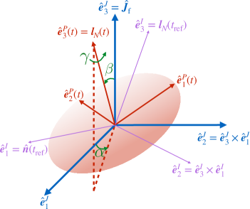
Figure 1: Frames used in the construction of the SEOBNRv5PHM model. The co-precessing frame (red) is constructed such that its $z$-axis is instantaneously aligned with the Newtonian angular momentum $\bm{l}_{N}(t)$ and can be described by the Euler angles $(\alpha,\beta,\gamma)$ with respect to $\bm{J}_{\rm f}$-frame (blue), while the source frame (purple) corresponds to the inertial frame defined by the initial Newtonian angular momentum $\bm{l}_{N}(t_{\rm ref})$ and unit separation vector $\hat{\bm{n}}(t_{\rm ref})$. For the SEOBNRv5PHM model we adopt the convention that at $t_{\rm ref}$, the source and co-precessing frames coincide.

We calculate the co-precessing frame inspiral-plunge GW waveform modes by evaluating the factorized, resummed non-precessing modes along the EOB dynamics described in Eqs. (10), with time-dependent projections of the spins $\left\{\bm{a}_{\pm}\cdot\bm{l}_{N},\bm{a}_{\pm}\cdot\bm{l},\bm{a}_{+}\cdot\bm{a}_{-},\bm{a}^{2}_{\pm}\right\}$. Following Ref. [148], in which an EOB non-precessing multipolar waveform (SEOBNRv5HM) calibrated to NR non-precessing simulations was developed, we include in the co-precessing frame of the SEOBNRv5PHM model the $\{(2,\pm 2),(2,\pm 1),(3,\pm 3),(3,\pm 2),(4,\pm 4),(4,\pm 3),(5,\pm 5)\}$ modes, and make the assumption $h^{P}_{l,-m}=(-1)^{l}h^{P*}_{l,m}$. As discussed in Sec. IIIB of Ref. [98], the inaccuracies due to neglecting mode asymmetries should remain modest, and are expected to be at most comparable to other modeling errors.

To assemble the inertial-frame modes, we first rotate $h_{\ell m}^{P}$ to the ${\bm{J}}_{\rm f}$-frame using $\bar{q}_{J\rightarrow P}$, and then from the ${\bm{J}}_{\rm f}$-frame to the source frame using $\bar{q}_{I\rightarrow J}$. To make contact with literature, it is useful to express these rotations in terms of Euler angles. Using the active ZYZ convention (see Fig. 1), the $J\rightarrow P$ rotation is given by

$$q_{J\rightarrow P}=e^{\alpha\hat{\bm{z}}/2}e^{\beta\hat{\bm{y}}/2}e^{\gamma\hat{\bm{z}}/2}.$$ (17)

In this formulation, the minimal rotation condition is given by $\dot{\gamma}=-\dot{\alpha}\cos\beta$ [143].

III.2 Merger-ringdown waveforms

After the coalescence, the description of a BBH system of two individual objects is no longer valid, and the EOB model builds the ringdown stage via a phenomenological model of the quasinormal modes (QNMs) of the remnant BHs, formed after the merger of the progenitors. The QNMs frequencies are tabulated functions of the final mass, $M_{f}$, and angular momentum $\bm{S}_{f}=M_{f}^{2}\bm{\chi}_{f}$ of the remnant BH [192]. The QNMs are defined with respect to the direction of the final spin, and thus, the description of the ringdown signal as a linear combination of QNMs, is formally valid only in an inertial frame with the z-axis parallel to $\bm{\chi}_{f}$.

Following Ref. [98], in SEOBNRv5PHM the attachment of the merger-rindown waveform is performed in the co-precessing frame. Therefore, we employ the merger-ringdown multipolar model developed for non-precessing BBHs (SEOBNRv5HM) in Ref. [148].

The calculation of the waveform in the inertial observer’s frame requires a description of the co-precessing frame Euler angles $\{\alpha(t),\beta(t),\gamma(t)\}$ which extends beyond merger. Here, we take advantage of a phenomenological prescription based on insights from NR simulations [193]. More specifically, it was shown that the co-precessing frame continues to precess roughly around the direction of the final angular momentum with a precession frequency, $\omega_{\rm prec}$, proportional to the difference between the lowest overtone of the $(2,2)$ and $(2,1)$ QNM frequencies, while the opening angle of the precessing cone, $\beta$, tends to decrease at merger. This phenomenology translates into the following expressions for the merger-ringdown angles in SEOBNRv5PHM,

$$\alpha^{\rm merger-RD} =\alpha(t_{\rm match})+\omega_{\rm prec}(t-t_{\rm match}),$$ (18)

$$\beta^{\rm merger-RD} =\beta(t_{\rm match}),$$ (19)

$$\gamma^{\rm merger-RD} =\gamma(t_{\rm match})-\omega_{\rm prec}(t-t_{\rm match})\cos\beta(t_{\rm match}),$$ (20)

where $t_{\rm match}$ is the time of attachment of the merger-ringdown model. We have also investigated non-constant post-merger extensions of the $\beta$ angle, such as the small opening angle approximation (see Eq. (24b) of Ref. [56]), but we find that such an approximation may degrade the faithfulness of the model to NR for certain configurations.

The behavior noticed in Ref. [193], describes prograde configurations, were the remnant spin is positively aligned with the orbital angular momentum at merger. However, to keep the model generic and accurate in a wide parameter space of mass ratios and spins, we extend the prescription to the retrograde case (negative alignment of the final spin with respect to the angular momentum at merger), which is typical for high mass-ratio binaries, when the total angular momentum $\bm{J}$ is dominated by the primary spin $\bm{S}_{1}$ instead of $\bm{L}$. While we keep imposing simple precession around the final spin at a rate $\omega_{\rm prec}\geq 0$ in our model, we distinguish two cases depending on the direction of the total angular momentum at merger $\bm{\chi}_{f}\sim\bm{J}_{\rm f}$ with respect to the final orbital angular momentum $\bm{L}_{f}$,

$$\omega_{\rm prec}=\left\{\begin{aligned} &\omega^{\rm QNM}_{22}(\chi_{f})-\omega^{\rm QNM}_{21}(\chi_{f})\quad\text{if}\quad\bm{\chi}_{f}\cdot\bm{L}_{f}>0\\ &\omega^{\rm QNM}_{2-1}(\chi_{f})-\omega^{\rm QNM}_{2-2}(\chi_{f})\quad\text{if}\quad\bm{\chi}_{f}\cdot\bm{L}_{f}<0\end{aligned}\right.,$$ (21)

where $\chi_{f}=|\bm{\chi}_{f}|$, and the QNM frequencies for negative $m$ are taken from the continous extension of the $m>0$, $\omega^{\rm QNM}_{lm}>0$ branch [192]. We stress that this prescription of the post-merger extension of the Euler angles for the retrograde case is much less tested than the prograde case due to the lack of NR simulations covering this region of parameter space, which also includes particular systems with transitional precession [17].

Following recent insights from NR of Ref. [194], where a correct prescription of the shift of the co-precessing QNM frequencies was developed, we compute in the SEOBNRv5PHM model the co-precessing frame QNM frequencies from the QNM frequencies in the $\bm{J}_{\rm f}$-frame as,

$$\omega^{\rm QNM,P}_{lm}=\omega^{\rm QNM,J}_{lm}-m(1-|\cos\beta(t_{\rm match})|)\omega_{\rm prec}.$$ (22)

Another essential aspect in the construction of the merger-rindown waveforms is the mapping from binary component masses and spins to the final mass and spin, required to evaluate the QNM frequencies of the remnant. Several groups have developed fitting formulas based on large sets of NR simulations (see Ref. [195] for a brief overview of the literature). To ensure agreement in the non-precessing limit with SEOBNRv5HM [148], we employ the fits for the final mass from Ref. [196], and the fits from Ref. [197] for the final spin.

The application of the fitting formulae for the final mass and spin requires choosing a time during the inspiral at which to evaluate the spins, as for precessing binaries the individual components of the spins vary with time. In the SEOBNRv5PHM model, we choose to evaluate the spins at a time corresponding to an orbital separation $r=10M$. Similarly as in Ref. [98], this choice is based on good agreement with NR configurations, and by the restriction that the smallest initial orbital separation must be $r>10.5M$ to ensure small initial eccentricities [97]. Additionally, this choice guarantees that a given physical configuration always produces the same waveform regardless of the initial starting frequency, as all configurations will pass through an orbital separation $r=10M$.

Finally, the inspiral-merger-ringdown GW modes in the inertial frame $h^{I}_{lm}$ are obtained by rotating the inspiral-merger-ringdown modes $h_{lm}^{P}$ from the co-precessing frame to the inertial observer’s frame using the expressions for the rotations in Appendix A of Ref. [97]. The inertial frame GW polarizations at a time $t$, and location in the sky of the observer $(\varphi_{0},\iota)$ can be expressed in terms of the $-2$-spin-weighted spherical harmonics, as follows

$$h^{\rm I}_{+}(t;\bm{\lambda},\varphi_{0},\iota)-ih^{\rm I}_{\times}(t;\bm{\lambda},\varphi_{0},\iota)=\sum_{\ell,m}{}_{-2}Y_{\ell m}(\varphi_{0},\iota)\,h^{\rm I}_{\ell m}(t;\bm{\lambda})\,,$$ (23)

where $\bm{\lambda}$ represents the set of intrinsic parameters (masses and spins), and $\{\varphi_{0},\iota\}$ the coalescence phase and the inclination angle of the signal.

III.3 Efficient calculation of the GW polarizations

For applications in which only the GW polarizations are required, as for most of the current parameter-estimation codes, we introduce an alternative and computationally more efficient method to obtain the polarizations directly in terms of the co-precessing $-2$-spin-weighted spherical harmonic modes. This involves rotating the spin-weighted spherical harmonic basis, instead of computing the full set of spin-weighted spherical harmonic modes in the inertial frame.

The inertial-frame (I-frame) modes are related to the co-precessing-frame (P-frame) modes by a time-dependent rotation from the co-precessing frame to the frame where the $z$-axis is aligned with the final angular momentum of the system ($\bm{J}_{\rm f}$-frame ), and a time-independent rotation from the $\bm{J}_{\rm f}$-frame to the final inertial frame

$$h^{\rm I}_{\ell m}(t)=\sum_{m^{\prime},m^{\prime\prime}}\Big{(}\textbf{R}^{\rm J\rightarrow I}\Big{)}_{m,m^{\prime}}\Big{(}\textbf{R}^{\rm P\rightarrow J}\Big{)}_{m^{\prime},m^{\prime\prime}}h^{\rm P}_{\ell m^{\prime\prime}}(t),$$ (24)

where $\textbf{R}^{\rm X\rightarrow Y}$ indicates the rotation operator from the frame $X$ to the frame $Y$, and the indices $m^{\prime},m^{\prime\prime}$ denote summation indices over the modes available in the co-precessing frame.

Factoring out the source orientation information from the spin-weighted spherical harmonic basis as a rotation of the basis

$${}_{-2}Y_{\ell m}(\varphi_{0},\iota)=\sum_{m^{\prime}}\Big{(}\textbf{R}^{\varphi_{0},\iota}\Big{)}_{m,m^{\prime}}{}_{-2}Y_{\ell m}(0,0),$$ (25)

the complete rotation of the basis functions from the co-precessing frame to the final inertial frame can be constructed composing the individual rotations as

$$\textbf{R}^{\rm P\rightarrow I}=\textbf{R}^{\varphi_{0},\iota}\textbf{R}^{\rm J\rightarrow I}\textbf{R}^{\rm P\rightarrow J},$$ (26)

with associated Euler angles $\{\alpha_{\rm P\rightarrow I},\beta_{\rm P\rightarrow I},\gamma_{\rm P\rightarrow I}\}$. Applying this rotation operator, the spin-weighted spherical harmonic basis can be written as

$$\sum_{m^{\prime}}\Big{(}\textbf{R}^{\rm P\rightarrow I}\Big{)}_{m,m^{\prime}}{}_{-2}Y_{\ell m}(0,0)=e^{2i\alpha_{\rm P\rightarrow I}}{}_{-2}Y_{\ell m}(\gamma_{\rm P\rightarrow I},\beta_{\rm P\rightarrow I}),$$ (27)

and the GW polarizations in the inertial frame can therefore be expressed as

$$h^{\rm I}_{+}(\varphi_{0},\iota;t)-ih^{\rm I}_{\times}(\varphi_{0},\iota;t)=e^{2i\alpha_{\rm P\rightarrow I}}\sum_{\ell,m}{}_{-2}Y_{\ell m}(\gamma_{\rm P\rightarrow I},\beta_{\rm P\rightarrow I})\,h^{\rm P}_{\ell m}(t).$$ (28)

Eq. (28) is only summed over the set of 7 co-precessing modes, and the computation of the complete rotation and its application to the basis functions is more efficient than the corresponding (double) rotation of the GW modes, which requires the rotation of 33 GW modes.

IV Performance of the multipolar precessing-spin effective-one-body waveform model

In this section we assess the accuracy of the multipolar precessing-spin SEOBNRv5PHM model by comparing it, as well as other models, to NR simulations of quasi-circular precessing-spin BBHs. Particularly, we consider state-of-the-art precessing-spin models within the EOB framework, such as SEOBNRv4PHM [98] and the public version of TEOBResumS-GIOTTO [102], and within the phenomenological approach, the frequency-domain IMRPhenomXPHM [52] (and in Appendix C the time-domain IMRPhenomTPHM [56] model). All the previous models, including SEOBNRv5PHM, are not calibrated to precessing-spin NR waveforms. We also investigate the validity and systematics of models by comparing them against the surrogate NRSur7dq4 [62] model. Finally, we assess the computational efficiency of the SEOBNRv5PHM model to be used for data analysis.

IV.1 Brief overview of the faithfulness function

The GW signal emitted by a quasi-circular precessing-spin BBH system depends on 15 parameters: the component masses, $m_{1,2}$ (or equivalently mass ratio $q$ and total mass $M$), the dimensionless spin vectors $\bm{\chi}_{1,2}(t)$, the direction of the observer from the source can be described by the angles $(\varphi_{0},\iota)$, the luminosity distance $d_{L}$, polarization angle $\psi$, the location in the sky of the detector $(\theta,\phi)$, and the time of arrival $t_{c}$. The strain in the detector caused by a passing GW can be expressed as

$$h(t)\equiv F_{+}(\theta,\phi,\psi)\ h_{+}(t;\iota,\varphi_{0},d_{L},\bm{\lambda},t_{\mathrm{c}})$$

$$+F_{\times}(\theta,\phi,\psi)\ h_{\times}(t;\iota,\varphi_{0},d_{L},\bm{\lambda},t_{\mathrm{c}})\,,$$ (29)

where $\bm{\lambda}=\{q,M,\bm{\chi}_{1,2}(t)\}$ is introduced to simplify the notation, and $F_{+,\times}$ are the antenna pattern functions [198, 199]. The strain in Eq. (IV.1) can be expressed in terms of an effective polarization angle $\kappa(\theta,\phi,\psi)$ as

$$h(t)=\mathcal{A}(\theta,\phi)(h_{+}\cos\kappa+h_{\times}\sin\kappa),$$ (30)

where the dependences of $\kappa$, $h_{+}$ and $h_{\times}$ have been removed to ease notation, and the definition of the coefficient $\mathcal{A}(\theta,\phi)$ can be found in Refs. [95, 98]. As discussed, the GW polarizations can be decomposed in the basis of $-2$-spin weighted spherical harmonics as

$$h_{+}-ih_{\times}=\sum_{l=2}^{\infty}\sum_{m=-l}^{m=+l}{}_{-2}Y_{lm}(\varphi_{0},\iota)h_{lm}(t;\bm{\lambda}),$$ (31)

where $h_{lm}(t;\bm{\lambda})$ are the GW multipolar modes.

We introduce the inner product between two waveforms, $h_{1}$ and $h_{2}$ [198, 199]

$$\left(h_{1},h_{2}\right)\equiv 4\ \textrm{Re}\int_{f_{\rm in}}^{f_{\rm max}}df\,\frac{\tilde{h}_{1}(f)\ \tilde{h}_{2}^{*}(f)}{S_{n}(f)},$$ (32)

where a tilde indicates Fourier transform, a star complex conjugation and $S_{n}(f)$ the power spectral density (PSD) of the detector noise. In this work, we employ for the PSD the LIGO’s “zero-detuned high-power” design sensitivity curve [200]. When both waveforms are in band we use $f_{\rm in}=10{\rm Hz}$ and $f_{\rm max}=2048{\rm Hz}$. For cases where this is not the case (e.g., the NR waveforms are used), we employ $f_{\rm in}=1.35f_{\rm peak}$, where $f_{\rm peak}$ corresponds to the peak amplitude of the frequency-domain strain of the signal, and the factor $1.35$ accounts for possible artifacts coming from the Fourier transform of the time domain waveforms.

To assess the agreement between two waveforms — for instance, the signal, $h_{s}$, and the template, $h_{t}$, observed by a detector, we define the faithfulness function [95, 98],

$$\mathcal{F}(M_{\textrm{s}},\iota_{\textrm{s}},{\varphi_{0}}_{\textrm{s}},\kappa_{\textrm{s}})=\max_{t_{c},{\varphi_{0}}_{t},\kappa_{t}}\left[\left.\frac{\langle h_{s}|h_{t}\rangle}{\sqrt{\langle h_{s}|h_{s}\rangle\langle h_{t}|h_{t}\rangle}}\right|_{\begin{subarray}{c}\iota_{\mathrm{s}}=\iota_{t}\\ \bm{\lambda}_{\mathrm{s}}(t_{\mathrm{s}}=t_{0_{\mathrm{s}}})=\bm{\lambda}_{t}(t_{t}=t_{0_{\mathrm{t}}})\end{subarray}}\right].$$ (33)

When comparing waveforms with higher-order multipoles  [95, 98, 53] a typical choice in Eq. (33) is to set the inclination angle of the template and the signal to be the same, while the coalescence time, azimuthal and effective polarization angles of the template, $(t_{0_{t}},\varphi_{0_{t}},\kappa_{t})$, are adjusted to maximize the faithfulness of the template. The maximizations over the coalescence time $t_{c}$ and coalescence phase ${\varphi_{0}}_{t}$ are performed numerically, while the optimization over the effective polarization angle $\kappa_{t}$ is done analytically as described in Ref. [201].

In Eq. (33) the condition $\bm{\lambda}_{\rm s}(t_{\rm s}=t_{0_{\rm s}})=\bm{\lambda}_{\rm t}(t_{\rm t}=t_{0_{\rm t}})$ enforces that the intrinsic properties (mass ratio $q$, total mass $M$, and spins $\bm{\chi}_{1,2}$) of the template waveform at $t=t_{0}$ (typically the start of the waveform) are the same as at its $t_{0}$. However, such identification of the same $t_{0}$ is not trivially satisfied between different waveforms, including NR and waveform models. As a consequence, several approaches can be applied to mitigate such a choice. For instance, in Ref. [98] $t_{0_{\rm t}}$ is chosen such that the time elapsed from $t_{0_{\rm s}}$ and $t_{0_{\rm t}}$ to the peak of the frame-invariant amplitude $\sum_{l,m}|h_{lm}|^{2}$ occurs at the same time for NR and SEOBNRv4PHM, while in Refs. [49, 98] numerical optimizations over the reference frequency of the waveform were performed for waveforms of the IMRPhenom family. Here, we instead optimize numerically over a rigid rotation $\delta\in[0,2\pi]$ of the in-plane spin components of the template $\{\chi^{\rm t}_{i,x},\chi^{\rm t}_{i,y}\}$ with $i=1,2$, at the reference frequency [52, 202], such that

$$\begin{split}\chi^{\rm t}_{i,x}&=\chi^{\rm s}_{i,x}\cos(\delta)-\chi^{\rm s}_{i,y}\sin(\delta),\\ \chi^{\rm t}_{i,y}&=\chi^{\rm s}_{i,x}\sin(\delta)+\chi^{\rm s}_{i,y}\cos(\delta),\quad i=1,2,\\ \end{split}$$ (34)

where $\{\chi^{\rm s}_{i,x},\chi^{\rm s}_{i,y}\}$ denote the in-plane spin components of the signal. This method, contrary to the procedure of optimizing over the reference frequency of the template, has unambiguous bounds for the parameters involved.

It is convenient to introduce the sky-and-polarization averaged faithfulness to reduce the dimensionality of the faithfulness function and express it in a more compact form [95, 98],

$$\overline{\mathcal{F}}(M_{\textrm{s}})=\frac{1}{8\pi^{2}}\int^{1}_{-1}d{(\cos\iota_{\textrm{s}})}\int^{2\pi}_{0}d{\varphi_{0}}_{\textrm{s}}\int^{2\pi}_{0}d\kappa_{\textrm{s}}\mathcal{F}(M_{\textrm{s}},\iota_{\textrm{s}},{\varphi_{0}}_{\textrm{s}},\kappa_{\textrm{s}}).$$ (35)

Another useful metric to assess the closeness between waveforms is the signal-to-noise (SNR)-weighted faithfulness [98]

$$\overline{\mathcal{F}}_{\mathrm{SNR}}(M_{\mathrm{s}})=\sqrt[3]{\frac{\int^{1}_{-1}d{(\cos\iota_{\textrm{s}})}\int_{0}^{2\pi}d\kappa_{\mathrm{s}}\int_{0}^{2\pi}d{\varphi_{0}}_{\mathrm{s}}\ \mathcal{F}^{3}(M_{\textrm{s}},\iota_{\textrm{s}},{\varphi_{0}}_{\textrm{s}},\kappa_{\textrm{s}})\ \mathrm{SNR}^{3}(\iota_{\textrm{s}},{\varphi_{0}}_{\textrm{s}},\kappa_{\textrm{s}})}{\int^{1}_{-1}d{(\cos\iota_{\textrm{s}})}\int_{0}^{2\pi}d\kappa_{\mathrm{s}}\int_{0}^{2\pi}d{\varphi_{0}}_{\mathrm{s}}\ \mathrm{SNR}^{3}(\iota_{\textrm{s}},{\varphi_{0}}_{\textrm{s}},\kappa_{\textrm{s}})}},$$ (36)

where the SNR is defined as

$$\mathrm{SNR}(\iota_{\textrm{s}},{\varphi_{0}}_{\textrm{s}},\theta_{\textrm{s}},\phi_{\textrm{s}},\kappa_{\textrm{s}},{d_{\mathrm{L}}}_{\mathrm{s}},\bm{\lambda}_{\mathrm{s}},{t_{c}}_{\mathrm{s}})\equiv\sqrt{\left(h_{\mathrm{s}},h_{\mathrm{s}}\right)}.$$ (37)

In Eq. (36) the weighting by the SNR takes into account the dependence on the phase and effective polarization of the signal at a fixed distance. Finally, we introduce the unfaithfulness or mismatch as

$$\overline{\mathcal{M}}_{\rm SNR}=1-\overline{\mathcal{F}}_{\rm SNR}.$$ (38)

IV.2 Assessment in modeling spin effects in EOB Hamiltonian

In Secs. II and III we have described the construction of the SEOBNRv5PHM model, here we assess the impact of several approximations in the description of the precessing-spin dynamics as well as in the waveform multipoles. Differently from the SEOBNRv4PHM model, in SEOBNRv5PHM the full precessing-spin Hamiltonian and spin equations are not evolved. By contrast, we build on recent waveform models, IMRPhenomTPHM [56] and TEOBResumS-GIOTTO [102], which couple a purely aligned-spin dynamics (only $\bm{a}_{\pm}\cdot\bm{l}_{N}$) with PN-expanded equations for the spins, angular-momentum and frequency. However, in the new SEOBNRv5PHM model there are significant differences with respect to previous approaches:

• The spin, velocity and angular momentum equations in SEOBNRv5PHM are fully PN-expanded in the velocity parameter $v$, and include SO and SS couplings through NNLO, thus differ from the ones employed in Refs. [146, 56, 102].

• The SO contributions to the angular momentum equations in SEOBNRv5PHM are consistent with the fully generic canonical Hamiltonian $H^{\rm prec}_{\rm EOB}$ [147] (i.e., they use the same spin-supplementary condition, and thus differ from the ones in Refs. [146, 56, 102]).

• In SEOBNRv5PHM, the orbital equations of motion are evolved using a partial precessing-spin EOB Hamiltonian, $H^{\rm pprec}_{\rm EOB}(\bm{l}^{2},\bm{a}_{\pm}\cdot\bm{l}_{N},\bm{a}_{\pm}\cdot\bm{l},\bm{a}_{+}\cdot\bm{a}_{-})$, which has all spin components (also orbit-averaged in-plane spin components instead of only $\bm{a}_{\pm}\cdot\bm{l}_{N}$).

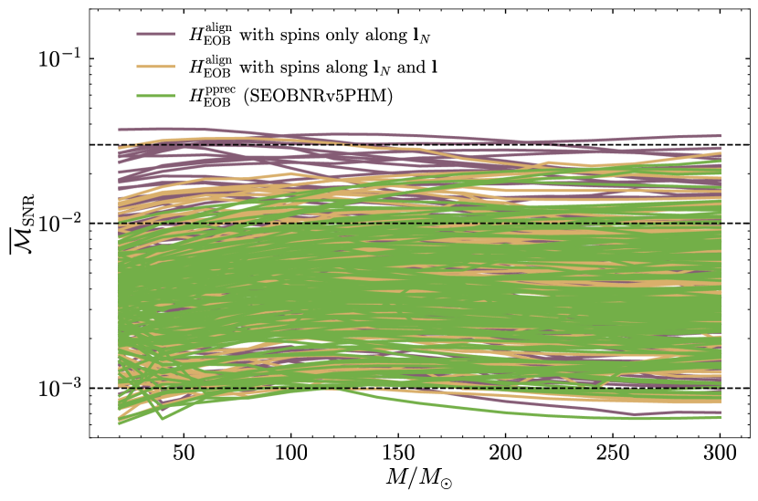
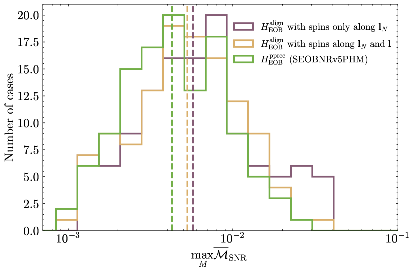
Figure 2: Left panel: Sky-and-polarization averaged, SNR-weighted unfaithfulness in the total mass range between $[20-300]M_{\odot}$ for an inclination $\iota=\pi/3$, of SEOBNRv5PHM with different prescriptions for the dynamics against the 118 highly precessing-spin NR simulations from Ref. [98]. The different prescriptions for the dynamics correspond to using the SEOBNRv5HM Hamiltonian, $H^{\rm align}_{\rm EOB}$, with the spins projected onto $\bm{l}_{N}$ (purple), using $H^{\rm align}_{\rm EOB}$ with the spins projected onto $\bm{l}_{N}$ and $\bm{l}$ (yellow), and using the partially precessing Hamiltonian $H^{\rm pprec}_{\rm EOB}$ of SEOBNRv5PHM (green), with the spins projected onto $\bm{l}_{N}$ and $\bm{l}$, see the main text for details. The dashed horizontal vertical lines correspond to the $10^{-3}$, $0.01$ and $0.03$ unfaithfulness values. Right panel: Distribution of the maximum unfaithfulness over the total mass range for each NR simulation considered in the left plot. The vertical dashed lines indicate the median values of the distribution.

In Figure 2 we assess the impact of these improvements in the treatment of the precessing-spin dynamics by computing the unfaithfulness of SEOBNRv5PHM with different prescriptions for the conservative dynamics against the set of 118 highly precessing BBH simulations from Ref. [98].

The different prescriptions for SEOBNRv5PHM correspond to 1) using the aligned-spin Hamiltonian $H^{\rm align}_{\rm EOB}$ of SEOBNRv5HM [147, 148] with the spins only projected onto $(\bm{a}_{\pm}\cdot\bm{l}_{N})$, such that the spin variables are computed like $a^{2}_{\pm}=(\bm{a}_{\pm}\cdot\bm{l}_{N})^{2}$ (i.e., a purely aligned-spin dynamics as in the TEOBResumS-GIOTTO [102] and IMRPhenomTPHM [56] models), 2) employing $H^{\rm align}_{\rm EOB}$ with a spin treatment consisting in using the full spin components for the scalar products (i.e. $a^{2}_{\pm}=(\bm{a}_{\pm}\cdot\bm{a}_{\pm})^{2}$), as well as the spins projected onto $\bm{l}$ in the spin-orbit sector, and onto $\bm{l}_{N}$ in the rest of the spin sector, and 3) using the partially precessing Hamiltonian $H^{\rm pprec}_{\rm EOB}$ of SEOBNRv5PHM with the latter treatment of the spins projections (see Appendix A). In the left panel of Fig. 2 we show the unfaithfulness as a function of the total mass of the binary, while in the right panel the distributions of the maximum unfaithfulness in the total-mass range are displayed. The results show that using the aligned-spin Hamiltonian with the projections of the spins onto $\bm{l}_{N}$ (i.e., a purely aligned-spin dynamics as in TEOBResumS and IMRPhenomT), leads to $95.8\%$ $(75.4\%)$ of cases with a maximum unfaithfulness over the total mass range considered of $[20,300]M_{\odot}$, lower than $3\%$ ($1\%$), while considering projections onto $\bm{l}_{N}$, $\bm{l}$ and the full spin-components entering the aligned-spin Hamiltonian improves the previous numbers to $99.2\%$ $(80.5\%)$, and it reduces significantly the tail of cases with unfaithfulness larger than $3\%$. Finally, keeping the latter treatment of the spin projections and using the partially precessing Hamiltonian, $H^{\rm pprec}_{\rm EOB}$, which includes in-plane spin effects in an orbit-average approximation for quasi-circular orbits (see Appendix A for details), leads to a further increase in accuracy with $100\%$ $(86.4\%)$ of cases with a maximum unfaithfulness below $3\%$ ($1\%$). As a consequence, the latter Hamiltonian and treatment of spin effects is the one that we adopt in the SEOBNRv5PHM model.

IV.3 Comparison against numerical-relativity waveforms

The accuracy of the SEOBNRv5PHM model is assessed by comparing it to the publicly available simulations of the SXS catalogue [150], as well as the 118 highly precessing-spin simulations produced in Ref. [98]. We also perform such a comparison for other state-of-the-art precessing-spin EOB waveform models, SEOBNRv4PHM and TEOBResumS-GIOTTO, as well as the phenomenological frequency-domain IMRPhenomXPHM model. (To ease the comparisons we compare against phenomenological IMRPhenomTPHM  model in Appendix C). In Fig. 3 we provide an overview of the NR simulations employed to assess the accuracy of the different models. The precessing-spin simulations considered here were produced with the SpEC code [203], and they correspond to the 118 SXS runs from Ref. [98], and 1425 simulations available in the public SXS catalog [150].

We start by comparing the unfaithfulness of the precessing-spin models against the set of 118 highly precessing-spin simulations including all the modes up to $l=5$ in the NR waveforms. The waveform modes included in the co-precessing frame for the different models is done consistently with Ref. [148] for the non-spinning approximants, and they are specifically $(\ell,|m|)=\{(2,2),(2,1),(3,3),(4,4),(5,5)\}$ for SEOBNRv4PHM, $(\ell,|m|)=\{(2,2),(2,1),(3,3),(3,2),(4,4),(4,3),(5,5)\}$ for SEOBNRv5PHM, $(\ell,|m|)=\{(2,2),(2,1),(3,3),(3,2),(4,4)\}$ for IMRPhenomXPHM and $(\ell,|m|)=\{(2,2),(2,1)(3,3)$ $(3,2),(3,1)$,$(4,4),(4,3),(4,2)\}$ for TEOBResumS-GIOTTO.

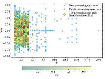
Figure 3: Parameter space coverage in $q-\chi_{\rm eff}-\chi_{\rm p}$ space for NR simulations used to build and validate the SEOBNRv5 models. For the non-precessing runs used in the construction of the SEOBNRv5HM model the color is fixed to blue (see Ref. [148] for details about these simulations). The precessing-spin runs follow a color map depending on the value of the effective spin parameter $\chi_{\rm p}$ at the reference time of the simulation. The set of precessing NR waveforms is built upon simulations from the public SXS catalog [150], as well as the 118 simulations from Ref. [98], which are highlighted with red diamonds to ease their visualization.

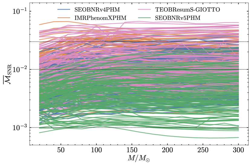
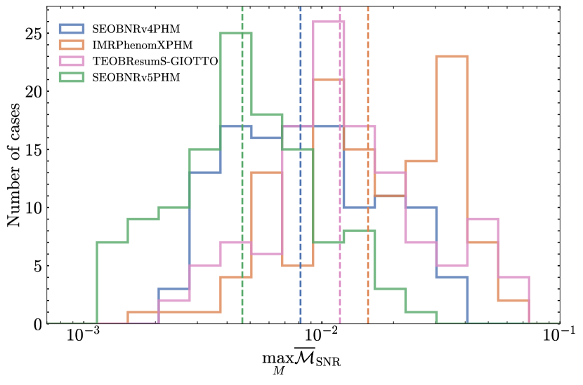
Figure 4: Left panel: Sky-and-polarization averaged, SNR-weighted unfaithfulness in the total mass range between $[20-300]M_{\odot}$ for an inclination $\iota=\pi/3$, between SEOBNRv4PHM (blue), IMRPhenomXPHM (orange), TEOBResumS-GIOTTO (pink) and SEOBNRv5PHM (green) against NR for the 118 highly precessing-spin BBH simulations from Ref. [98]. The dashed horizontal vertical lines correspond to the $10^{-3}$, $0.01$ and $0.03$ unfaithfulness values. Right panel: Distribution of the maximum unfaithfulness over the total mass range for each NR simulation considered in the left plot. The vertical dashed lines indicate the median values of the distribution.

In the left panel of Fig. 4 the unfaithfulness is shown as a function of total mass, $[20-300]M_{\odot}$, for each NR simulation, while in the right panel the distribution of the maximum unfaithfulness over the total mass range is displayed. The two panels of Fig. 4 show that the phenomenological model, IMRPhenomXPHM, and the EOB model TEOBResumS-GIOTTO, have a tail of large unfaithfulness reaching $\sim 7\%$. Precisely, they have $78.3\%$ $(38.3\%)$ and $83.3\%$ $(44.9\%)$ of cases with a maximum unfaithfulness, in the total mass range considered, below $3\%$ $(1\%)$, respectively. This tail of large unfaithfulness is not present in the SEOBNRv4PHM and SEOBNRv5PHM models, and it is consistent with the fact that both models include effects due to the evolution of the in-plane spin components in the co-precessing frame dynamics. More specifically, the SEOBNRv4PHM model has $96.6\%$ $(57.6\%)$ of cases with maximum unfaithfulness, in the total mass range considered, below $3\%$ $(1\%)$, while these numbers increase to $100\%$ $(85.6\%)$ for the SEOBNRv5PHM model, which has lower unfaithfulness (higher accuracy) than SEOBNRv4PHM. We suspect this is due to the more accurate underlying aligned-spin model, SEOBNRv5HM [148], as well as the new improvements included in SEOBNRv5PHM, such as the shift in the co-precessing QNM frequencies, described in Secs. II and III.

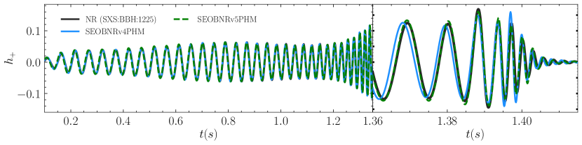
Figure 5: Time-domain comparison of the SEOBNRv5PHM and SEOBNRv4PHM models to the NR waveform PrecBBH000001 from Ref. [98] with mass ratio 1.25, black-hole spin magnitudes 0.8 and total mass $M=60M_{\odot}$. The source parameters are $\iota_{s}=\pi/3$, $\phi_{s}=\pi$, $\kappa_{s}=0$. The NR waveform includes all the multipoles with $l\leq 5$. Both waveform models resemble accurately the features of the NR waveform at the inspiral, merger and ringdown, with a more faithful agreement of SEOBNRv5PHM which translates into an unfaithfulness of $0.69\%$, while for SEOBNRv4PHM it increases to $1.1\%$.

In Fig. 5 we show the polarizations of SEOBNRv5PHM and SEOBNRv4PHM for the precessing NR simulation PrecBBH000001 with mass ratio 1.25, spin magnitudes $\chi_{i}\equiv|\bm{\chi}_{i}|=0.8$, total mass $60M_{\odot}$ and all the modes $l\leq 5$. Specifically, we plot the plus polarization, $h_{+}$, leaving out the overall constant amplitude. We note that SEOBNRv5PHM reproduces more accurately the features of the NR waveform at merger and ringdown, which translates into an unfaithfulness of $0.69\%$ against the NR waveform, while for SEOBNRv4PHM the unfaithfulness is $1.1\%$.

Approximant	SEOBNRv4PHM	SEOBNRv5PHM	IMRPhenomXPHM	TEOBResumS-GIOTTO
median $\max_{M}\overline{\mathcal{M}}_{\rm SNR}$	$7.49\cdot 10^{-3}$	$4.75\cdot 10^{-3}$	$14.35\cdot 10^{-3}$	$11.47\cdot 10^{-3}$
$\%$ cases with $\max_{M}\overline{\mathcal{M}}_{\rm SNR}<1\%$	$60.8\%$	$84.4\%$	$38.3\%$	$44.9\%$
$\%$ cases with $\max_{M}\overline{\mathcal{M}}_{\rm SNR}<3\%$	$95.3\%$	$99.8\%$	$78.3\%$	$83.3\%$

Table 1: Summary of the sky-and-polarization averaged, SNR-weighted unfaithfulness in the total mass range between $[20-300]M_{\odot}$ for an inclination $\iota=\pi/3$, between different precessing-spin approximants and the 1543 SXS NR simulations from Refs. [150, 98]. The table shows the median of the maximum unfaithfulness across total mass, and the percentage of cases with mismatches below $1\%$ and $3\%$.

We now turn to exploring the broader parameter space by computing the unfaithfulness against a set of 1543 precessing-spin NR waveforms (1425 public + 118 highly precessing configurations above). In Fig. 6 we show the unfaithfulness as a function of the total mass of the system for each model against all the simulations. Additionally, we highlight the simulations with the largest unfaithfulness for each waveform model in each panel. The simulations with larger unfaithfulness differ depending on the waveform approximant considered. For the EOB models they correspond to high mass ratios $q=4$ and high in-plane spin components where the modeling approximations are expected to perform worse, while the phenomenological model presents the largest unfaithfulness for an equal-mass simulation with high-in plane component.

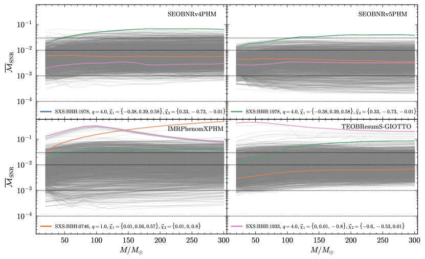
Figure 6: Sky-averaged SNR weighted unfaithfulness as a function of the total mass of the system $[20,300]M_{\odot}$, of the SEOBNRv4PHM model (top left panel), the SEOBNRv5PHM model (top right panel), the IMRPhenomXPHM model (left bottom panel) and TEOBResumS-GIOTTO (right bottom panel), against 1543 precessing-spin SXS simulations.The simulations with the highest unfaithfulness for each model are highlighted in each panel.

The results from Fig. 6 indicate that the SEOBNRv5PHM model has lower values of unfaithfulness with respect to the rest of the models. The information in Fig. 6 is more quantitatively represented in Fig. 7 as a violin plot of the distribution of unfaithfulness of the different models against NR for each total mass considered between $[20-300]M_{\odot}$. We note that the trend in the unfaithfulness is similar to the one for the 118 highly precessing-spin simulations. The IMRPhenomXPHM model has the largest tails of unfaithfulness reaching $10\%$, followed by the TEOBResumS-GIOTTO model, which generally has lower unfaithfulness than IMRPhenomXPHM as shown in Ref. [102]. The SEOBNRv4PHM model gives an even lower unfaithfulness, while the distributions of the SEOBNRv5PHM model have less support at high unfaithfulness than the rest of the models and lower median values for all the total masses considered with respect to the next more accurate model, SEOBNRv4PHM. A more quantitative analysis of the unfaithfulness against NR can be found in Table 1, which reveals that SEOBNRv5PHM has $99.8\%$ ($84.4\%$) cases with a maximum unfaithulness, in the total mass range considered, below $3\%$ ($1\%$). These numbers reduce to $95.3\%$ ($60.8\%$) for SEOBNRv4PHM, to $83.3\%$ $(44.9\%)$ for TEOBResumS-GIOTTO and to $78.3\%$ $(38.3\%)$ for IMRPhenomXPHM.

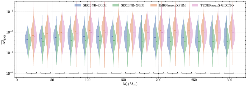
Figure 7: Distribution of the sky-and-polarization averaged, SNR-weighted unfaithfulness as a function of binary’s total mass for inclination $\iota=\pi/3$, between SEOBNRv4PHM (blue), SEOBNRv5PHM (green), IMRPhenomXPHM (orange) and TEOBResumS-GIOTTO (pink) against NR for 1543 quasi-circular precessing-spin BBH simulations. For each total mass considered the distributions of SEOBNRv4PHM and SEOBNRv5PHM, and IMRPhenomXPHM and TEOBResumS-GIOTTO have been shifted in the x-axis by $4M_{\odot}$ from the total mass value used to compute the unfaithfulness to ease the visualization of the results. The bracket indicates the total mass value used for the unfaithfulness calculation. In each distribution the median value is highlighted with thicker lines.

Finally, we provide a more complete picture of the accuracy of the different models against NR in the quasi-circular limit by incorporating to our precessing results the unfaithfulness corresponding to 441 non-precessing SXS NR waveforms computed in Ref. [148]. Fig. 8 shows violin plots of the maximum, median and minimum unfaithfulness distributions of the different waveform models considered in the aligned-spin, precessing-spin case and with the combined distributions. A thorough discussion of the accuracy of the different models in the non-precessing case can be found in [148], but we remark that the new aligned-spin SEOBNRv5HM model presents the lowest unfaithfulness distribution when compared to the other models. As discussed above, in the precessing case the SEOBNRv5PHM model leads to the lowest unfaithfulness values followed closely by the SEOBNRv4PHM model. We also observe that the lack of calibration to precessing-spin NR waveforms causes a shift in the unfaithfulness of the precessing-spin models (with respect to the nonprecessing models) towards larger values. This points out that in order to increase further the accuracy of the models in the precessing-spin case, calibration to NR precessing waveforms is required, which we leave to the future.

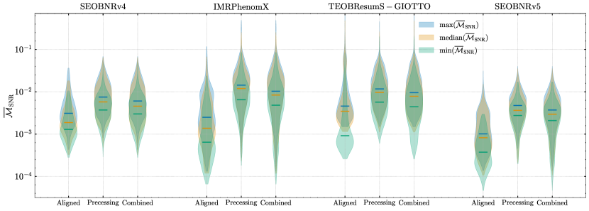
Figure 8: Distribution of maximum (blue), median (orange) and minimum (green) sky-and-polarization averaged, SNR-weighted unfaithfulness over the binary’s total mass range $[20-300]M_{\odot}$ for inclination $\iota=\pi/3$, between the different waveform families (SEOBNRv4, IMRPhenomX, TEOBResumS-GIOTTO and SEOBNRv5) against NR for aligned spins (Aligned), precessing spins (Precessing) and combining the two previous distributions (Combined). The non-precessing NR simulations correspond to the 441 cases presented in Ref. [148], while the precessing NR simulations correspond to the 1543 cases used in Fig. 6. In the violin plots the median values of the distributions are highlighted with thicker lines.

IV.4 Comparison against other precessing-spin waveform models

We now study the performance of the SEOBNRv5PHM model in a larger parameter space. First we compute the unfaithfulness of SEOBNRv5PHM against the NR surrogate model NRSur7dq4 [62], which includes all $l\leq 4$ waveform multipoles, in the region in which it was built, that is mass ratios $q\in[1,4]$, spin magnitudes up to 0.8 and total masses larger than $\leavevmode\nobreak\ 60M_{\odot}$. Specifically, we generate a set of 5000 cases uniformly distributed in mass ratios $q\in[1,4]$ and effective precessing-spin parameter $\chi_{p}$ [176], with spin magnitudes up to $0.8$ and initial geometric frequency of $M\omega=0.023$, large enough such that all the configurations have a length compatible with the one of the surrogate waveforms. We also compute the unfaithfulness of the state-of-the-art precessing-spin models, SEOBNRv4PHM, IMRPhenomXPHM and TEOBResumS-GIOTTO, against the NRSur7dq4 model.

The results of such study are summarized in Fig. 9, where in the left panel the median and the 95th percentile of the unfaithfulness, as a function of the total mass of the binary are shown, while in the right plot the distributions of the maximum unfaithfulness, over the total mass range $[20-300]M_{\odot}$, are displayed. We find that the behavior of the unfaithfulness resembles those of the comparisons against the NR waveforms in Figs. 4 and 7. All the models have median unfaithfulness below $1\%$ with the SEOBNRv5PHM model showing the lowest median  of $0.39\%$ unfaithfulness values. We note that the median of unfaithfulness of SEOBNRv5PHM is followed very closely by the other models, with the SEOBNRv4PHM model being the closest one. The difference between the SEOBNR models and the IMRPhenomXPHM and TEOBResumS-GIOTTO models is likely a consequence of neglecting the in-plane spin effects in the orbital dynamics in the co-precessing frame. As described in Sec. II, these effects are introduced in SEOBNRv5PHM through the partially precessing Hamiltonian, $H^{\rm pprec}_{\rm EOB}$. Furthermore, the increase in accuracy of SEOBNRv5PHM with respect to SEOBNRv4PHM can be understood due to the more accurate underlying co-precessing waveform model (SEOBNRv5HM), as well as the improvements discussed in Sec. III. More quantitatively, we find that for SEOBNRv5PHM $100\%$ $(90.1\%)$ of cases have a maximum unfaithfulness, in the total mass range considered, against the NRSur7dq4 model below $3\%$ $(1\%)$, while these numbers reduce to $98.7\%$ $(79.5\%)$ for SEOBNRv4PHM, $89.4\%$ $(62.8\%)$ for IMRPhenomXPHM  and $96.1\%$ $(66\%)$ for TEOBResumS-GIOTTO. For all the models the cases with high unfaithfulness correspond to configurations with mass ratios $q\sim 4$ and $\chi_{p}\sim 0.8$, which is the boundary region of calibration of the NRSur7dq4 model, and where the effects of spin precession are stronger in the waveform, as already seen in previous comparisons to the NR surrogate in Refs. [98, 102].

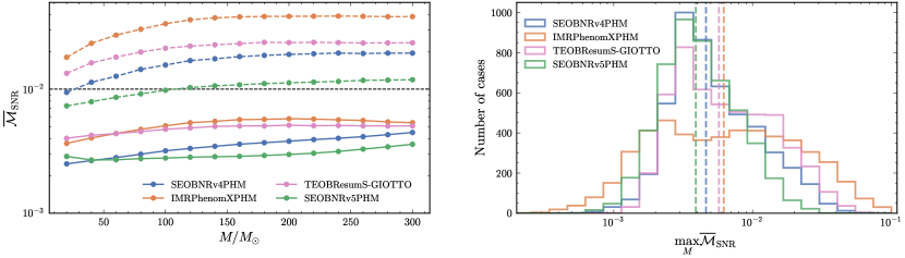
Figure 9: Sky-and-polarization-averaged, SNR-weighted unfaithfulness as a function of the total mass of the binary for inclination $\iota_{s}=\pi/3$, among the NRSur7dq4 model and the SEOBNRv4PHM (blue), IMRPhenomXPHM (orange), TEOBResumS-GIOTTO (pink) and SEOBNRv5PHM (green) models for 5000 randomly distributed precessing-spin configurations. Left: The solid (dashed) lines show the median (95th percentile) as a function of the total mass. Right: Distribution of maximum unfaithfulness over all the total masses considered. The vertical dashed lines indicated the median values of the distributions.

Finally, we also examine the behavior of the precessing models in a wider parameter space outside the region of calibration of the underlying aligned-spin models, and where there are no precessing-spin NR simulations available. For this purpose we consider 5000 configurations randomly distributed in mass ratios $q\in[1,20]$ and uniformly distributed in the effective precessing-spin $\chi_{p}$ parameter up to 0.99, for inclination $\iota_{s}=\pi/3$, with an initial starting geometric frequency of $M\omega=0.022$, and compute the unfaithfulness, $\overline{\mathcal{M}}_{\rm SNR}$, using the IMRPhenomXPHM as a signal, and the SEOBNRv5PHM model as the template waveform. Figure 10 shows the unfaithfulness as a function of mass ratio ($q$), effective spin parameter ($\chi_{\mathrm{eff}}$), and effective precessing-spin parameter ($\chi_{\mathrm{p}}$). We find that for mass ratios $q<5$, $96.84\%$ ($41.3\%$) of cases have a maximum unfaithfulness, in the total mass range $[20,300]M_{\odot}$, below $10\%$ $(1\%)$. The unfaithfulness increases significantly with mass ratio and spins, with the highest unfaithfulness values at the largest mass ratios $q\sim 20$, and effective spin precessing parameter $\chi_{\mathrm{p}}\sim 0.99$. In particular, when considering $q\leq 20$ we find that $59.19\%$ $(13.45\%)$ cases with maximum unfaithfulness, in the total mass range considered, below $10\%$ $(1\%)$. These unfaithfulness comparisons and the large differences between models point out the necessity to populate this challenging region of high mass ratio and high spins with NR simulations, which can be used to validate distinct waveform models, as well as to improve their accuracy by incorporating this NR information into them.

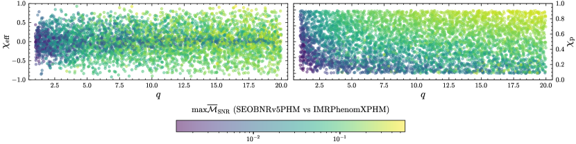
Figure 10: Maximum sky-and-polarization-averaged unfaithfulness weighted by the SNR over the total mass range $[20-300]M_{\odot}$ between SEOBNRv5PHM and IMRPhenomXPHM for 5000 random configurations with inclination $\iota_{s}=\pi/3$. The unfaithfulness grows with increasing mass ratio and spin magnitude values, and it can reach very large values for mass ratios $q\sim 20$ and $\chi_{\mathrm{p}}\sim 1$.

IV.5 Computational performance

In previous sections we have demonstrated the accuracy of the SEOBNRv5PHM model with respect to NR waveforms and predictions of other state-of-the-art waveforms models. Another key aspect to test is the computational efficiency of the model, as parameter-estimation runs with standard stochastic samplers require of the order of $10^{7}-10^{8}$ or more waveform evaluations (see e.g. Refs. [204, 205, 206]). Therefore, computational efficiency is a key feature for the model to be useful for the analysis of GW signals or Bayesian inference studies.

The SEOBNRv5PHM model is part of the fifth generation of SEOBNR models implemented in a high-performance Python package pySEOBNR [168]. As described in Ref. [168], the pySEOBNR infrastructure offers a simple and modular procedure to develop highly accurate and computationally efficient waveform models. This new Python infrastructure moves the development of the SEOBNR family from the highly efficient, but more rigid C-99 LALSuite [207] libraries to a more flexible and modular Python framework.

In this section we asses the computational efficiency of the SEOBNRv5PHM model implemented in pySEOBNR, by timing the waveform generation and comparing it to other state-of-the-art time-domain multipolar precessing-spin models (SEOBNRv4PHM, IMRPhenomTPHM and TEOBResumS-GIOTTO). We consider binary’s configurations with mass ratios $q=1,3,10$, dimensionless spins $\bm{\chi}_{1}=[0.5,0,0.8]$, $\bm{\chi}_{2}=[0,0.5,0.3]$, total mass range $M\in[10,100]M_{\odot}$ at a starting frequency $f_{\rm start}=10$Hz. The results of the walltimes to generate the waveforms are shown in Fig. 11, where we are including all the modes up to $l=4$, and a maximum frequency consistent with the Nyquist criterion satisfied for all the multipoles considered . The outcome of the benchmark demonstrates the significant increase in speed of the SEOBNRv5PHM model with respect to the previous generation SEOBNRv4PHM. For the arbitrary configurations considered for the benchmarks, we observe more than an order of magnitude improvement in speed. The substantial increase in speed for SEOBNRv5PHM is a consequence, not only of the fast and efficient implementation in the pySEOBNR infrastructure, but also to the use of the PN-expanded spin and angular-momentum evolution equations, Eqs. (13), which allow the use of the PA approximation [165, 167] in the SEOBNRv5PHM model. The PA approximation reduces the computational cost of evaluating the inspiral waveform as it replaces solving numerically the ordinary differential equations at every timestep of the EOB inspiral by an iterative procedure over a coarser radial grid (see Appendix B for details of the implementation in SEOBNRv5PHM). Besides the PA approximation, the SEOBNRv5PHM model also implements an efficient calculation of the polarizations as described in Se. III.3, which translates into a further increase in speed at lower total masses, where the computational cost of generating the waveform comes from the interpolation of the waveform multipoles into a constant time grid . This can be seen in Fig.  11, where the SEOBNRv5PHM model outperforms the TEOBResumS-GIOTTO and IMRPhenomTPHM models at low total masses, while at high total masses where the interpolation of the modes is a subdominant operation in terms of computational cost, the TEOBResumS-GIOTTO and IMRPhenomTPHM perform faster. IMRPhenomTPHM is substantially faster at high total masses than the rest of the models, due to the fact that it is only integrating the evolution equations for the spins (i.e., no integration of the orbital dynamics as in the SEOBNRv4PHM, SEOBNRv5PHM and TEOBResumS-GIOTTO models), and the waveform is evaluated using analytical closed expressions. In summary, the SEOBNRv5PHM model has a comparable speed to current state-of-the-art precessing-spin models, and it is in general between $8-20$ times faster than the SEOBNRv4PHM model, and thus it can be used as a standard tool for data analysis as demonstrated in Sec. V.

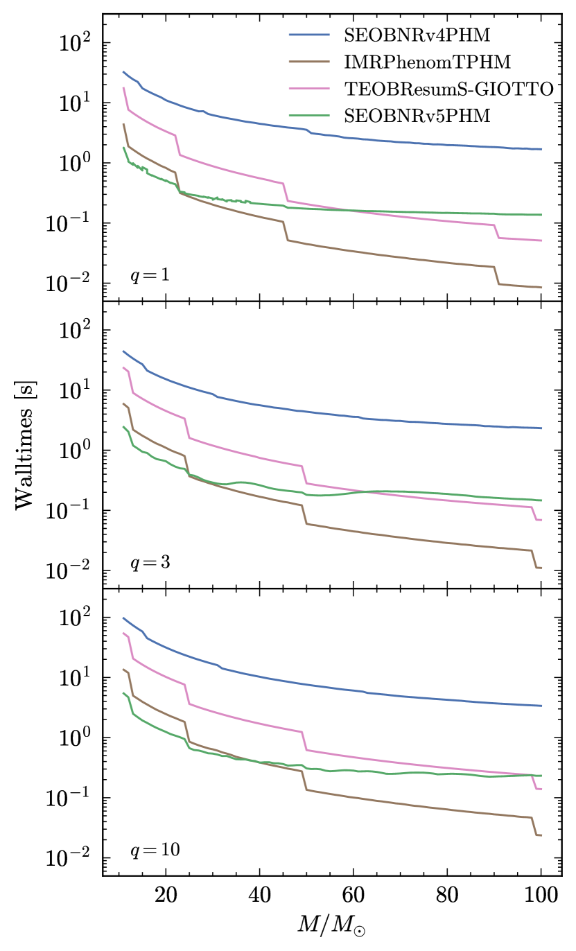
Figure 11: Walltimes of the SEOBNRv4PHM, IMRPhenomTPHM, TEOBResumS-GIOTTO and SEOBNRv5PHM models for a configuration with dimensionless spins $\bm{\chi}_{1}=[0.5,0,0.8]$, $\bm{\chi}_{2}=[0,0.5,0.3]$, total mass range $M\in[10,100]M_{\odot}$, starting frequency $f_{\rm start}=10$Hz and three different mass ratios 1 (top panel), 3 (mid panel) and 10 (bottom panel).

V Bayesian analysis with multipolar precessing waveform models

The main application of the SEOBNRv5PHM waveform model is the Bayesian inference of source parameters of GWs emitted by BBHs. Thus, we now assess how the accuracy of SEOBNRv5PHM quantified in Sec. IV through the unfaithfulness metric affects parameter-estimation studies. We perform first a synthetic NR signal injection into detector noise, in particular in zero-noise, which is equivalent to averaging over many noise realizations, to assess possible biases coming from waveform inaccuracies and avoid any biases introduced by a random noise realization. Then, we perform a re-analysis of 6 real GW events detected by the LVK collaboration: GW150914, GW190412, GW190521, GW190814, GW191109 and GW200129, and we compare with results from the literature.

V.1 NR-injection recovery

In this section we assess the accuracy of the SEOBNRv5PHM model in parameter estimation by injecting a synthetic NR signal corresponding to the NR waveform SXS:BBH:0165 from the public SXS catalog, with mass ratio $q=6$, source-frame total mass $M=95M_{\odot}$ and BH’s dimensionless spin vectors defined at 20Hz of $\bm{\chi}_{1}=[-0.06,0.78.-0.4]$ and $\bm{\chi}_{2}=[0.08,-0.17,-0.23]$. This BBH system is strongly precessing, and it is one of the worst cases in terms of unfaithfulness for SEOBNRv5PHM, reaching $2\%$ for the injected total mass.

For this injection we choose the inclination with respect to the line of sight of the BBH to be $\iota=0.69$ rad, to emphasize the effect of higher order modes. The injected coalescence and polarization phases are $\phi=0.6$ rad and $\psi=0.33$ rad, respectively. The sky-position is defined by its right ascension of 3.81 rad and declination of 0.63 rad at a geocentric time of 1126259600 s. The luminosity distance to the source is chosen to be 650 Mpc, which produces a three-detector (LIGO Hanford, LIGO Livingston and Virgo) network-SNR of $19.4$ when using the LIGO and Virgo PSD at design sensitivity [200].

For the parameter estimation study we employ parallel Bilby [208], a highly parallelized version of the Bayesian inference Python package Bilby [209, 210], using the recommended LVK’s setting for the number of auto-correlation times $\mathrm{nact}=50$, number of live points $\mathrm{nact}=2048$, and setting the remaining sampling parameters to their default values. We choose a uniform prior in inverse mass ratio and chirp mass, with ranges $1/q\in[0.05,1]$ and $\mathcal{M}\in[15,45]M_{\odot}$. The priors on the dimensionless spin vectors are uniform in magnitude $a_{i}\in[0,0.99]$, and isotropically distributed in the unit sphere for the spin directions. The luminosity distance prior is uniform in distance $\propto d_{L}$ as we are interested in the intrinsic ability of the models in recovering the parameters, since a prior uniform in the comoving-frame of the source $\propto d_{L}^{2}$ requires selecting a specific cosmology to compute the redshift [211], which may introduce an effect on the estimated posterior. The rest of the priors are set according to Appendix C of Ref. [2]. We perform the injection-recovery with SEOBNRv5PHM and IMRPhenomXPHM in order to compare the performance of both models with a highly precessing signal. We note that IMRPhenomXPHM has an unfaithfulness of $\sim 12\%$ against the SXS NR-injected waveform, thus we expect some biases in the recovered parameters.

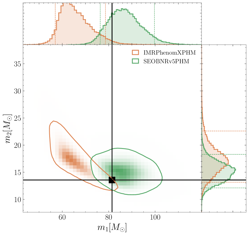
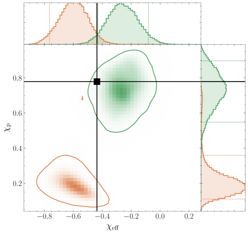
Figure 12: 2D and 1D posterior distributions for some relevant parameters measured from the synthetic BBH signal with mass ratio $q=6$, total source-frame mass of $95M_{\odot}$, dimensionless spins of the BHs $\bm{\chi}_{1}=[-0.06,0.78.-0.4]$ and $\bm{\chi}_{2}=[0.08,-0.17,-0.23]$ defined at 20Hz. The inclination with respect to the line of sight of the binary is $\iota=0.69$ rad. The other parameters are specified in the text and in Table 2. The signal waveform is a NR waveform from the public SXS catalog SXS:BBH:0165. In the 2D posteriors the solid contours represent the $95\%$ credible intervals and black dots show the values of the parameters of the injected signal. In the 1D posteriors they are represented by dashed and solid vertical lines, respectively. The parameter estimation is performed with the SEOBNRv5PHM model (green) and the IMRPhenomXPHM model (orange). Left: Component masses in the detector frame. Right: Effective spin parameters, $\chi_{\mathrm{eff}}$ and $\chi_{\mathrm{p}}$.

In Fig. 12 we summarize the parameter-estimation results of the injection. We report the marginalized 1D and 2D posteriors for the detector-frame component masses $m_{1}$ and $m_{2}$, and the effective spin parameters, $\chi_{\mathrm{eff}}$ and $\chi_{\mathrm{p}}$. In Table 2 we provide the values of the injected parameters and the median of the inferred posterior distribution with the $90\%$ confidence intervals for both models. The results show that SEOBNRv5PHM is able to recover the component masses within the $90\%$ confidence intervals, while IMRPhenomXPHM presents a significant bias in the primary mass, and the injected values are at the boundary of the 2D $95\%$ credible interval. For the effective spin parameters, both models present a biased result for the effective spin parameter $\chi_{\mathrm{eff}}$, but the precessing effective spin parameter $\chi_{\mathrm{p}}$ is highly biased in IMRPhenomXPHM towards lower values, while SEOBNRv5PHM recovers an almost unbiased result. Moreover, the injected point is inside the 2D $95\%$ credible interval for SEOBNRv5PHM, while IMRPhenomXPHM predicts a region with lower precessing spins and highly anti-aligned spins. From Table 2 we observe that the spin tilt angles, $\theta_{1,2}$, are recovered within the $90\%$ confidence interval by SEOBNRv5PHM, but the phenomenological model IMRPhenomXPHM presents biases for both parameters. In terms of recovered matched filter SNR, SEOBNRv5PHM recovers higher values in the three detectors with respect to IMRPhenomXPHM, which is consistent with the higher Bayes factor obtained by SEOBNRv5PHM. This example shows the ability of SEOBNRv5PHM to model more accurately precessing signals in comparison to IMRPhenomXPHM, likely due to the inclusion of in-plane spin information in the conservative dynamics of the model. It should be noted that there are some parameters for which SEOBNRv5PHM presents small biases, such as the effective-spin parameter $\chi_{\mathrm{eff}}$ and the tilt angle of the orbital plane $\theta_{\text{JN}}$, which might be expected since this simulation provides one of the highest unfaithfulness for the model of $\sim 2\%$, while for the IMRPhenomXPHM model the unfaithfulness increases to $\sim 12\%$, which explains the larger biases in more parameters than SEOBNRv5PHM. However, more studies will be needed in a larger region of the binary’s parameter space to assess the efficiency of SEOBNRv5PHM  in capturing spin precession.

Parameter	Injected value	IMRPhenomXPHM	SEOBNRv5PHM
$M/M_{\odot}$	$95.02$	$82.51^{+9.6}_{-5.27}$	$101.59^{+12.96}_{-9.56}$
$\mathcal{M}/M_{\odot}$	$21.85$	$27.76^{+3.34}_{-1.88}$	$29.3^{+3.74}_{-3.14}$
$q$	$0.167$	$0.27^{+0.12}_{-0.1}$	$0.17^{+0.05}_{-0.04}$
$\chi_{\text{eff}}$	$-0.437$	$-0.6^{+0.16}_{-0.17}$	$-0.26^{+0.18}_{-0.17}$
$\chi_{\text{p}}$	$0.779$	$0.19^{+0.17}_{-0.08}$	$0.74^{+0.16}_{-0.19}$
$\theta_{1}$	$2.11$	$3.01^{+0.09}_{-0.21}$	$1.97^{+0.25}_{-0.25}$
$\theta_{2}$	$2.46$	$1.5^{+0.57}_{-0.56}$	$1.4^{+1.11}_{-0.93}$
$\theta_{\text{JN}}$	$1.28$	$0.81^{+0.43}_{-0.28}$	$0.46^{+0.21}_{-0.22}$
$d_{L}$	$1200$	$1444^{+223}_{-237}$	$1374^{+325}_{-248}$
$\phi_{\text{ref}}$	$1.2$	$3.66^{+1.19}_{-1.13}$	$3.01^{+2.86}_{-2.61}$
$\psi$	$0.7$	$2.4^{+0.52}_{-1.79}$	$0.89^{+0.84}_{-0.57}$
$\rho^{\mathrm{H1}}_{\mathrm{mf}}$	$13.92$	$13.55^{+0.1}_{-0.19}$	$13.68^{+0.09}_{-0.16}$
$\rho^{\mathrm{L1}}_{\mathrm{mf}}$	$16.03$	$15.61^{+0.11}_{-0.2}$	$15.75^{+0.1}_{-0.17}$
$\rho^{\mathrm{V1}}_{\mathrm{mf}}$	$6.66$	$6.47^{+0.09}_{-0.28}$	$6.52^{+0.06}_{-0.23}$
$\log{\mathcal{BF}}$		$194.33\pm 0.19$	$205.65\pm 0.18$

Table 2: Injected and median values of the posterior distributions for the synthetic NR injection, corresponding to the NR simulation SXS:BBH:0165 of the public SXS catalog, recovered with IMRPhenomXPHM and SEOBNRv5PHM. The binary parameters correspond to the total mass $M$, chirp mass $\mathcal{M}$, mass ratio $q$, effective spin parameter $\chi_{\text{eff}}$, effective precessing-spin parameter $\chi_{\text{p}}$, tilt angles $\theta_{1,2}$, angle between the total angular momentum and the line of sight $\theta_{\text{JN}}$, luminosity distance $d_{L}$, coalescence phase $\phi_{\text{ref}}$, polarization angle $\psi$, matched-filtered SNR for LIGO-Hanford/Livingston and Virgo detectors $\rho^{\mathrm{H1},\mathrm{L1},\mathrm{V1}}_{\mathrm{mf}}$, and signal-versus-noise log Bayes factor $\log{\mathcal{BF}}$.

V.2 Real events

In this section we re-analyze 6 GW events recorded by the LIGO and Virgo detectors [2, 7, 8]: GW150914, GW190412, GW190521, GW190814, GW191109 and GW200129. We employ strain data from the Gravitational Wave Open Source Catalog (GWOSC) [212] and the released PSD and calibration envelopes included in the Gravitational Wave Transient Catalogs GWTC-2.1 [7] and GWTC-3 [8], and their respective parameter-estimation samples releases.

We perform the analysis using the parameter-estimation code Bilby [209], and the nested sampler dynesty [213] using the acceptance-walk method, which is well-suited for executing on a multicore single-computing node, and we perform the run for GW190521 with the parameter-estimation code parallel Bilby [208] as the nested sampler settings for this event are more expensive and the parallelization of this code ensures results in a short timescale. The list of parameter-estimation runs and the main settings are specified in Table 3, together with the runtime and the number of cores employed. We find that results can be obtained using Bilby on just one computing node within days.

GW event sampler	Data settings		Sampler settings		Computing resources	Runtime
	srate (Hz)	seglen (s)	naccept/ nact	nlive	cores$\times$nodes
GW150914 Bilby	2048	8	60	1000	$64\times 1$	1d 17h
GW190412 Bilby	4096	8	60	1000	$64\times 1$	4d 3h
GW190521 Bilby	2048	8	60	1000	$64\times 1$	1d 17h
GW190521 parallel Bilby	2048	8	30	8192	$64\times 8$	3d 4h
GW190814 Bilby	4096	32	60	1000	$64\times 1$	5d 23h
GW191109 Bilby	1024	8	60	1000	$64\times 1$	2d 1h
GW200129 Bilby	2048	8	60	1000	$64\times 1$	2d 21h

Table 3: Settings and evaluation time for the different parameter estimation runs on real GW events with the SEOBNRv5PHM model. Sampling rate (srate) and data segment duration (seglen) are specified in the data settings, while the number of accepted MCMC-chains naccept for bi and number of live points nlive are specified in the sampler settings (for the GW190521 parallel Bilby run, the number quoted is the number of auto-correlation times). The time reported is walltime, while the total computational cost in CPU hours can be obtained multiplying this time by the reported number of CPU cores employed.

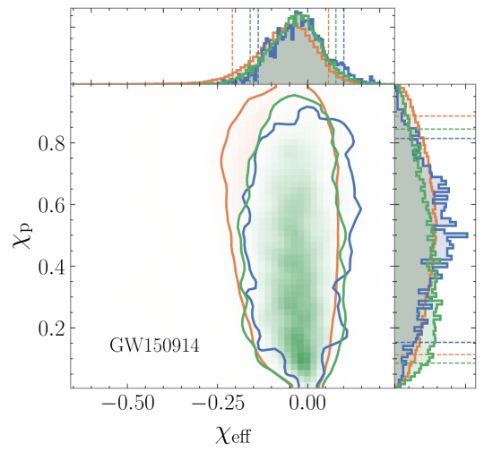
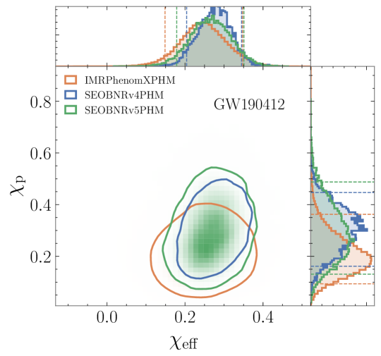
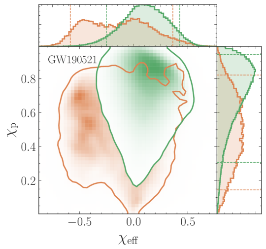
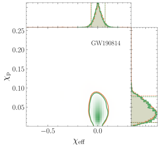
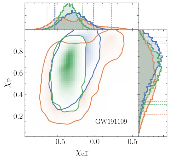
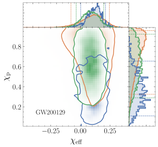
Figure 14: Effective-spin parameters $\chi_{\text{eff}}$ and $\chi_{\text{p}}$ inferred for the GW events re-analysed with SEOBNRv5PHM. Comparisons are presented with SEOBNRv4PHM (when available) and IMRPhenomXPHM from GWTC-2.1 [7] and GWTC-3 [8] catalogs, except for GW190412 for which we present the SEOBNRv4PHM from the discovery paper [214] as in Fig. 13.

In Figure 13 we summarize the results for the source component masses for the 6 re-analyzed events with SEOBNRv5PHM and we compare with results from the IMRPhenomXPHM model released in GWTC-2.1 and the previous generation SEOBNR model SEOBNRv4PHM (when available) also from GWTC-2.1 (obtained with the parameter-estimation code RIFT [169, 170]), except for the event GW190412 in which we show the SEOBNRv4PHM results from the discovery paper [214] (obtained with parallel Bilby) due to a better convergence of the posteriors than in the GWTC-2.1 catalog [7]. Similarly, in Figure 14 we summarize the results for the effective spin parameters $\chi_{\text{eff}}$ and $\chi_{\text{p}}$. In general, we observe broad consistency between our results and the GWTC results, but differences are stronger in some of the events, with IMRPhenomXPHM being, in general, more in tension with our results than SEOBNRv4PHM.

For GW150914 we observe good consistency between the SEOBNRv5PHM and SEOBNRv4PHM models, however the source mass posteriors are less constrained for IMRPhenomXPHM.

For GW190412, the first confident mass-asymmetric event reported by the LIGO-Virgo collaboration [214], we observe a better agreement between the time-domain models SEOBNRv5PHM and SEOBNRv4PHM, which also are consistent with results from the phenomenological time-domain model IMRPhenomTPHM from Ref. [215]. For this event, the higher-mode content is important, and the more accurate precessing dynamics provides a more reliable multipolar structure of the waveforms, therefore the tension with IMRPhenomXPHM can be explained by the fact that the precessing description contains more approximations in this model.

The GW190521 signal is particularly interesting, with only 4 cycles in band in the detectors, thus being consistent with a merger-ringdown dominated signal. It has been attributed to a variety of physical systems, from eccentric binaries [216, 217], non-spinning hyperbolic capture [202] and head-on collision of exotic compact objects [218]. Under the conservative assumption of a quasi-circular binary system, we observe differences with respect to the IMRPhenomXPHM results from GWTC-2.1. We have compared our results with the re-analysis of Ref. [219] in which the phenomenological time-domain model IMRPhenomTPHM was employed using LALInference MCMC [220], and in Fig. 15 we present the 2D distribution of mass-ratio and effective spin $\chi_{\text{eff}}$. We observe a better consistency in the results with IMRPhenomTPHM, in particular the mass asymmetric support for the posterior is correlated with positive effective spin, instead of negative effective spin as the results from IMRPhenomXPHM suggest. The reason for the tension with IMRPhenomXPHM can be explained by the fact that this Fourier-domain model lacks a description of the effective precessing motion of the ringdown signal, which is present (although in an approximate way) in SEOBNRv5PHM and IMRPhenomTPHM.

The next event we re-analyze is GW190814, a computationally challenging signal due to its low chirp mass and high-mass asymmetry, compatible with a heavy neutron star black-hole system. For this event we find very good agreement between the IMRPhenomXPHM results from GWTC-2.1 and our results, in essentially all the parameters. The good agreement can be explained by the fact that this signal is consistent with a non-spinning configuration, and in the small spin-magnitude region the systematics between models is less severe, due to the underlying calibration of the non-precessing baselines. It is worth noting that the result for this event can be obtained within days with SEOBNRv5PHM employing parallel Bilby.

We also re-analyze GW191109, an interesting signal with support for negative effective spin and non-negligible in-plane spin. For this event, we observe a slightly better consistency for the source component masses between SEOBNRv4PHM and IMRPhenomXPHM, although the spin distribution is more consistent between SEOBNRv4PHM and SEOBNRv5PHM. Note that that the IMRPhenomXPHM results present multimodality in some parameters, like the effective spin parameter $\chi_{\rm eff}$, while this feature is not present both in the SEOBNRv4PHM and SEOBNRv5PHM results, therefore the more accurate modeling of the precessing dynamics could help in solving this degeneracy. Another interesting feature is that SEOBNRv5PHM seems to produce more constrained parameters than the other two models.

The last event we re-analyze is GW200129, which has been-claimed to be the first confident precessing-spin detection [221] (although there are some concerns with data quality issues and glitch substraction that were discussed in Ref. [222]). Our results do not recover a high support for high precessing spin values, although the support is greater in SEOBNRv5PHM than in SEOBNRv4PHM results.

Finally, in Fig. 16, we present the posterior distribution of the network matched-filter SNR $\rho^{\text{N}}_{\text{mf}}$ for some of the events, computed from the results of SEOBNRv5PHM, as well as IMRPhenomXPHM that we obtain running this model with the same settings as SEOBNRv5PHM. We can observe that in general greater SNR values are recovered with SEOBNRv5PHM, in particular for the events that show higher support for precession. This is likely due to the better description of the precessing dynamics included in SEOBNRv5PHM, as well as the modeling of the precessing ringdown, which is absent in the Fourier-domain model IMRPhenomXPHM. This, together with the differences we have observed in the parameter posteriors, emphasizes the importance of using several accurate models such as SEOBNRv5PHM for production analysis of GW events.

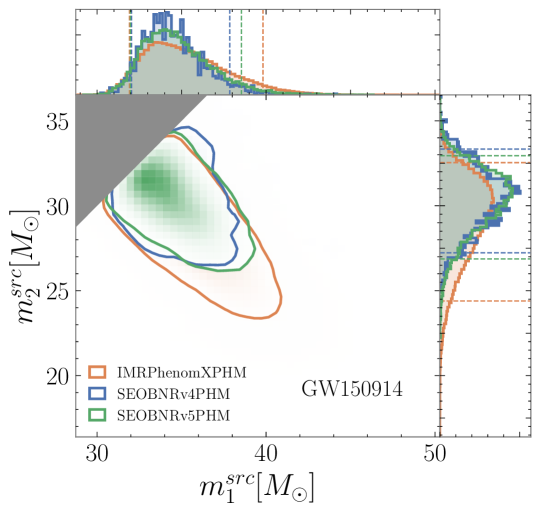
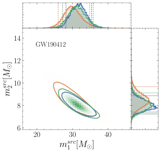
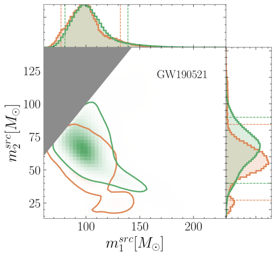
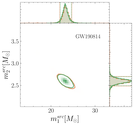
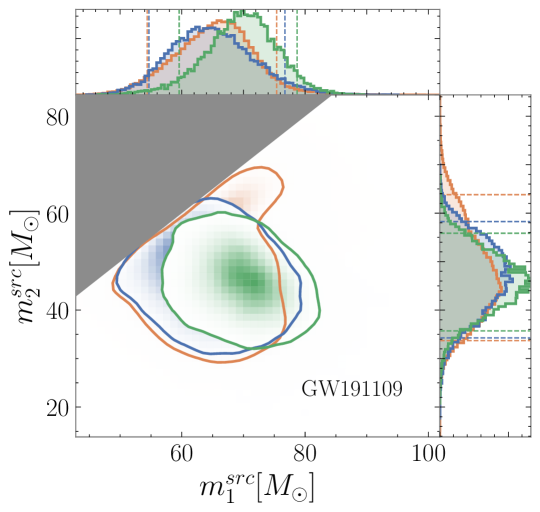
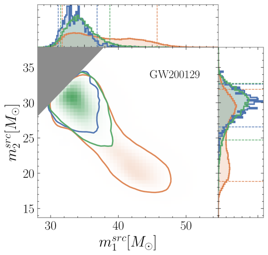
Figure 13: Component masses in the source-frame inferred for the real GW events re-analysed with SEOBNRv5PHM. Comparisons are presented with SEOBNRv4PHM (when available) and IMRPhenomXPHM from GWTC-2.1 [7] and GWTC-3 [8] catalogs, except for GW190412 for which we present the SEOBNRv4PHM from the discovery paper [214], since the convergence of the posteriors is larger than in the GWTC-2.1 catalog.

Figure 15: Comparison of mass-ratio and effective spin parameter inferred for GW190521 between SEOBNRv5PHM and the phenomenological models IMRPhenomTPHM from Ref. [219] and IMRPhenomXPHM from GWTC-2.1 [7].

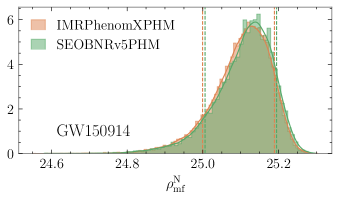
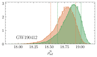
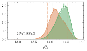
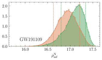
Figure 16: Distribution of network matched-filter SNR inferred for some of the GW events re-analysed with SEOBNRv5PHM. Comparisons are presented with IMRPhenomXPHM results obtained with the same settings and data as the SEOBNRv5PHM results.

.

VI Conclusions

In this paper we have developed and validated the multipolar precessing-spin SEOBNRv5PHM model, of the fifth generation of SEOBNR models. This work is the culmination of a series of papers developing the SEOBNRv5 models ahead of the fourth observing of the LVK Collaboration.

The SEOBNRv5 models are built upon the most recent analytical PN results and improved resummations for the Hamiltonian [223, 91, 147], the RR force and waveform modes [224, 225], including information from second-order gravitational self-force [226, 153] in the modes/RR force. The new analytical information and improvements in the conservative dynamics are derived in Ref. [147], while the inclusion of second order self-force results in the RR force and modes of SEOBNRv5 is obtained in Ref. [153]. All these new analytical improvements are combined with input from NR waveforms to improve the calibration of the non-precessing SEOBNRv5HM model in Ref. [148]. The NR calibration in the aligned-spin sector is extended to 442 NR waveforms, in addition to 13 Teukolsky waveforms. The multipolar SEOBNRv5HM model includes the $(2,2),(2,1),(3,3),(4,4),(5,5)$ plus the $(3,2),(4,3)$ modes for which the mode-mixing during ringdown is modelled, and it improves substantially the accuracy of the SEOBNR family against non-precessing NR waveforms [148].

This modeling effort is developed within a new Python infrastructure pySEOBNR [168], which offers more flexibility in including new analytical information, it is highly modular and it produces faster and more efficient SEOBNR models than the current ones in LALSuite [207].

More specifically, regarding the SEOBNRv5PHM model developed here, following previous precessing SEOBNR models [93, 98], we have built such a model twisting up the non-precessing waveforms of SEOBNRv5HM [148] from the co-precessing frame [141, 142, 143, 144, 145] to the inertial frame. With respect to the previous SEOBNR model, SEOBNRv4PHM [98], which has been used in LVK data analysis [7, 8], the new model: 1) does not evolve the EOB equations for the spins, but building on previous works [54, 101, 102] decouples the spin evolution equations from the evolution of the orbital dynamics allowing for the specification of a reference frequency distinct from the starting frequency of the evolution, 2) employs PN-expanded EOB spin evolution equations derived from the generic SEOBNRv5 Hamiltonian in an orbit-average approximation [147], 3) evolves the conservative dynamics using a partially precessing Hamiltonian, $H^{\rm pprec}_{\rm EOB}$, which includes in-plane spin terms in an orbit average and reduces to the SEOBNRv5HM Hamiltonian in the aligned-spin limit, 4) employs a more accurate aligned-spin two-body dynamics, since in the non-precessing limit it reduces to SEOBNRv5HM, 5) includes in the co-precessing frame two new modes $(3,\pm 2)$ and $(4,\pm 3)$, instead of only the $(2,\pm 2),(2,\pm 1),(3,\pm 3),(4,\pm 4),(5,\pm 5)$, 6) applies the PA scheme [165] to the EOB orbital evolution, which increases the efficiency of the model, 7) implements an efficient calculation of the polarizations based on the rotation of the basis of -2 spin-weighted spherical harmonics, which further accelerates the evaluation of the model, and 8) incorporates latest insights from NR waveforms by properly rotating the quasi-normal mode frequencies [194].

The improvement in accuracy between SEOBNRv5PHM and SEOBNRv4PHM is evident from Figure 4, where we have compared these models, as well as other state-of-the-art precessing-spin models (IMRPhenomXPHM, IMRPhenomTPHM and TEOBResumS-GIOTTO) to the public SXS catalog of 1425 precessing-spin NR waveforms, and the 118 SXS NR waveforms from Ref. [98]. When comparing to the highly precessing 118 simulations from Ref. [98], the SEOBNRv5PHM provides the highest accuracy with respect to NR waveforms (see Fig. 6), as it includes effects of in-plane spin components in its dynamics, unlike IMRPhenomXPHM, IMRPhenomTPHM and TEOBResumS-GIOTTO, while having a more accurate description of the co-precessing waveforms through the non-precessing SEOBNRv5HM model than SEOBNRv4PHM. When turning to a broader comparison and including all the 1543 SXS precessing-spin NR waveforms available, we have found that for the SEOBNRv5PHM model, $99.8\%$ ($84.4\%$) of cases have a maximum unfaithfulness value, in the total mass range $[20,300]M_{\odot}$, below $3\%$ ($1\%$). These numbers reduce to $95.3\%$ ($60.8\%$) for SEOBNRv4PHM, to $83.3\%$ $(44.9\%)$ for TEOBResumS-GIOTTO, to $91.6\%$ $(62.4\%)$ for IMRPhenomTPHM and to $78.3\%$ $(38.3\%)$ for IMRPhenomXPHM. We have also investigated the accuracy of the previous models, which are not calibrated to precessing-spin NR waveforms, against the NR surrogate NRSur7dq4 model by computing the unfaithfulness for 5000 configurations in the parameter space of the calibration of the surrogate model ($q\in[1-4]$, and $a_{1,2}\in[0,0.8]$). The configurations have been uniformly distributed in the effective precessing-spin parameter, $\chi_{p}$, to increase the number of configurations with highly precessional effects. We have found in Fig. 9 that SEOBNRv5PHM provides the lowest unfaithfulness against the surrogate model, with $100\%$ $(90.1\%)$ cases with maximum unfaithfulness, over the total mass range considered, below $3\%$ $(1\%)$, while these numbers reduce to $98.7\%$ $(79.5\%)$ for SEOBNRv4PHM, $89.4\%$ $(81.4\%)$ for IMRPhenomXPHM and $96.1\%$ $(66\%)$ for TEOBResumS-GIOTTO. The largest values of unfaithfulness against the surrogate model occur at high mass ratios and high values of the in-plane spin components, where the in-plane spin effects and mode asymmetries play an important role in the description of the waveforms. We have also compared SEOBNRv5PHM against IMRPhenomXPHM in a larger region of parameter space $q\in[1,20]$ and $\chi_{p}\in[0,0.99]$ outside the region of calibration of the underlying aligned-spin models. We have found that the largest differences occur at mass ratios larger than 4 and spin magnitudes larger than 0.8 (see Fig. 10). These results are consistent with the differences found in the comparisons of non-precessing models in Ref. [148], and highlight the need to improve the parameter-space coverage of the NR waveforms combined with improved analytical information in the spinning sector, such as gravitational self-force, so that the accuracy of the models can be further improved in these challenging regions of the parameter space.

The improvement in accuracy of the SEOBNRv5PHM model is also accompanied by an improvement in the speed of the model with respect to SEOBNRv4PHM. The acceleration in waveform evaluation of the model is a consequence of several factors: 1) its implementation in the high-performance pySEOBNR Python package [168], which allows to incorporate new analytical information combined with NR calibration in a flexible, modular and efficient way, 2) the PA routine, which accelerates the evaluation of the two-body dynamics (see Appendix B), and 3) an efficient procedure to compute the polarizations as described in Sec. III.3. As a result, we find that SEOBNRv5PHM is overall $\sim 8-20$ times faster than SEOBNRv4PHM, and comparable in speed to other state-of-the-art time-domain precessing-spin models (TEOBResumS-GIOTTO and IMRPhenomTPHM).

Given the high accuracy and computational efficiency of SEOBNRv5PHM, we have performed a Bayesian inference study on mock signals and real GW events detected by the LVK Collaboration. We have first investigated how the modeling inaccuracy impacts the inference of parameters by injecting a synthetic NR signal into a network of LIGO-Virgo detectors at design sensitivity. We have injected in zero noise a precessing-spin NR waveform (SXS:BBH:0165) with mass ratio 6, total mass 95 $M_{\odot}$, SNR 19.4, inclination $0.69$ with respect to the line of sight, and recovered it with SEOBNRv5PHM and IMRPhenomXPHM. The unfaithfulness values of these models against the synthetic signal is $2\%$ for SEOBNRv5PHM and $12\%$ for IMRPhenomXPHM. The results are summarized in Fig. 12 and Table 2. We have found that the recovery of the parameters with SEOBNRv5PHM does not produce significant biases, except for the effective spin parameter, for which the injected value lies at the boundary of the $90\%$ credible intervals, while the rest of the binary parameters are accurately recovered. While in the case of the IMRPhenomXPHM model a $12\%$ value of unfaithfulness translates into larger biases in several parameters, like the component masses or the effective precessing-spin parameter. A more comprehensive Bayesian inference study will be needed to quantify the modeling inaccuracies and systematics, and how they translate into biases in the inference of binary parameters. Here, new methods of Bayesian inference through machine learning techniques, like DINGO [171, 172, 173], may offer an alternative and efficient method to perform large-scale injection campaigns and assess waveform systematics with a significant reduction of its computational cost. We leave such waveform systematics studies using Bayesian inference methods for future work.

Besides injection studies, we have demonstrated that SEOBNRv5PHM can be used as a standard tool in Bayesian inference studies of real GW events. We have reanalyzed several GW events (GW150914, GW190412, GW190521, GW190814, GW191109 and GW200129) detected by the LVK Collaboration in the first and third observing runs, with two different standard stochastic samplers serial Bilby [209] and parallel Bilby [208]. We have found that the parameters inferred by SEOBNRv5PHM are consistent with the ones obtained in the literature for most of the events. For instance, in the case of the massive GW190521, we find consistency in the recovery of the mass ratio and effective spin parameter with other time-domain precessing models in the literature, while for GW200129, consistently with SEOBNRv4PHM, we do not find support for high precession as claimed in Ref. [221] using the NRSur7dq4 model. Furthermore, we find that for all the events considered in this paper SEOBNRv5PHM recovers systematically more SNR than the IMRPhenomXPHM model (see Fig. 16). The SEOBNRv5PHM model results have been obtained in a few days when using parallel Bilby, and on the order of a week when using serial Bilby (see Table 3). This makes SEOBNRv5PHM a standard tool that can be used with a variety of stochastic samplers, and we plan in the future to extend the Bayesian inference study presented here, including the machine-learning code DINGO, to all the GW events detected during the third-observing run [227].

Finally, the SEOBNRv5PHM model is not calibrated to precessing-spin NR waveforms, which limits its accuracy. To overcome this limitation, calibration to NR waveforms in the conservative dynamics, as well in the waveform modes with the inclusion of mode asymmetries will be developed in the future. In this context, the pySEOBNR infrastructure provides an ideal framework to incorporate such improvements, as well as other physical effects, such as eccentricity and tidal effects, which have been already incorporated in SEOBNRv4 models [108, 111, 112, 134, 114, 115], and that we are in the process of implementing in the SEOBNRv5 models. Further improvements for the near future concern with the adoption of the SEOBNRv5 models to perform theory agnostic tests of GR [228, 229, 230], as well as developing SEOBNR waveforms in specific beyond-GR theories and calibrating/comparing them to beyond-GR NR waveforms of BBHs [231, 232, 233, 234, 235].

Appendix A Precessing-spin effective Hamiltonian

In this Appendix, we provide the partial-precession Hamiltonian derived in Ref. [147], which reduces to the Hamiltonian of SEOBNRv5HM [148] in the aligned-spin limit and includes orbit-average in-plane spin components for quasi-circular orbits. The effective Hamiltonian is given by

$$H_{\text{eff}}^{\text{pprec}} =\frac{Mp_{\phi}\bm{l}\cdot(g_{a_{+}}\bm{a}_{+}+g_{a_{-}}\delta\bm{a}_{-})+\text{SO}_{\text{calib}}+\left\langle G_{a^{3}}^{\text{pprec}}\right\rangle}{r^{3}+a_{+}^{2}(r+2M)}$$

$$\quad+\bigg{[}A^{\text{pprec}}\,\bigg{(}\mu^{2}+B_{p}^{\text{pprec}}\frac{p_{\phi}^{2}}{r^{2}}+\left(1+B_{np}^{\text{pprec}}\right)(\bm{n}\cdot\bm{p})^{2}$$

$$\qquad\qquad+B_{npa}^{\text{Kerr\,eq}}\frac{p^{2}_{\phi}(\bm{l}\cdot\bm{a}_{+})^{2}}{r^{2}}+Q^{\text{pprec}}\bigg{)}\bigg{]}^{1/2},$$ (39)

where the gyro-gravitomagnetic factors are the same as in the aligned-spin case, which are given by Eq. (28) of Ref. [147], and the SO calibration term is given by

$$\text{SO}_{\text{calib}}=\nu d_{\text{SO}}\frac{M^{4}}{r^{3}}p_{\phi}\bm{l}\cdot\bm{a}_{+}.$$ (40)

with the same value of $d_{\text{SO}}$ as in the aligned-spin model [148]. The cubic-in-spin term $\left\langle G_{a^{3}}^{\text{pprec}}\right\rangle$ reads

$$\left\langle G_{a^{3}}^{\text{pprec}}\right\rangle =p_{\phi}\delta(\bm{l}\cdot\bm{a}_{-})\Bigg{\{}\frac{M}{r^{2}}\Bigg{[}\frac{a_{+}^{2}}{4}-\frac{5}{24}(\bm{l}_{N}\cdot\bm{a}_{+})^{2}\Bigg{]}$$

$$\qquad-\frac{p_{\phi}^{2}}{8\mu^{2}r^{3}}\left(a^{2}_{+}-(\bm{l}_{N}\cdot\bm{a}_{+})^{2}\right)\Bigg{\}}$$

$$\quad+p_{\phi}(\bm{l}\cdot\bm{a}_{+})\Bigg{\{}\frac{p_{\phi}^{2}}{\mu^{2}r^{3}}\left[\frac{\delta}{4}\left[\bm{a}_{+}\cdot\bm{a}_{-}-(\bm{l}_{N}\cdot\bm{a}_{+})(\bm{l}_{N}\cdot\bm{a}_{-})\right]\right.$$

$$\quad\qquad\left.-\frac{1}{8}\left(a^{2}_{+}-(\bm{l}_{N}\cdot\bm{a}_{+})^{2}\right)\right]$$

$$\qquad+\frac{M}{r^{2}}\Bigg{[}-\frac{5a_{+}^{2}}{8}+\frac{3}{8}(\bm{l}_{N}\cdot\bm{a}_{+})^{2}-\delta\frac{5}{8}(\bm{a}_{+}\cdot\bm{a}_{-})$$

$$\quad\qquad+\delta\frac{5}{6}(\bm{l}_{N}\cdot\bm{a}_{+})(\bm{l}_{N}\cdot\bm{a}_{-})\Bigg{]}\Bigg{\}}.$$ (41)

The potential $B_{npa}^{\text{Kerr\,eq}}$ in Eq. (A) is the same as in the Kerr Hamiltonian for equatorial orbits, and is given by

$$B_{npa}^{\text{Kerr\,eq}}=-\frac{1+2M/r}{r^{2}+a_{+}^{2}(1+2M/r)}.$$ (42)

The other potentials $A^{\text{pprec}}$, $B_{p}^{\text{pprec}}$, $B_{np}^{\text{pprec}}$, and $Q^{\text{pprec}}$ include nonspinning and SS PN terms, and read:

$$A^{\text{pprec}} =\frac{a_{+}^{2}/r^{2}+A_{\text{noS}}+A_{\text{SS}}^{\text{prec}}+\left\langle\tilde{A}_{\text{SS}}^{\text{in\,plane}}\right\rangle}{1+(1+2M/r)a_{+}^{2}/r^{2}},$$ (43)

$$B_{p}^{\text{pprec}} =1+\left\langle\tilde{B}_{p,\text{SS}}^{\text{in\,plane}}\right\rangle,$$

$$B_{np}^{\text{pprec}} =-1+a_{+}^{2}/r^{2}+A_{\text{noS}}\bar{D}_{\text{noS}}+B_{np,\text{SS}}^{\text{prec}},$$

$$Q^{\text{pprec}} =Q_{\text{noS}}+Q_{\text{SS}}^{\text{prec}},$$

where the nonspinning contributions $A_{\text{noS}}$, $\bar{D}_{\text{noS}}$ and $Q_{\text{noS}}$ are given by Eqs. (21)–(25) of Ref. [147], while the SS correctionsread

$$A_{\text{SS}}^{\text{prec}} =\frac{M^{2}}{r^{4}}\left[\frac{9a_{+}^{2}}{8}-\frac{5}{4}\delta\bm{a}_{-}\cdot\bm{a}_{+}+a_{-}^{2}\left(\frac{\nu}{2}+\frac{1}{8}\right)\right]+\frac{M^{3}}{r^{5}}\left[a_{+}^{2}\left(-\frac{175\nu}{64}-\frac{225}{64}\right)+\delta\bm{a}_{-}\cdot\bm{a}_{+}\left(\!\frac{117}{32}-\frac{39\nu}{16}\right)+a_{-}^{2}\left(\!\frac{21\nu^{2}}{16}-\frac{81\nu}{64}-\frac{9}{64}\right)\right],$$ (44a)

$$B_{np,\text{SS}}^{\text{prec}} =\frac{M}{r^{3}}\left[a_{+}^{2}\left(3\nu+\frac{45}{16}\right)-\frac{21}{8}\delta\bm{a}_{-}\cdot\bm{a}_{+}+a_{-}^{2}\left(\frac{3\nu}{4}-\frac{3}{16}\right)\right]$$

$$\quad+\frac{M^{2}}{r^{4}}\left[a_{+}^{2}\left(-\frac{1171\nu}{64}-\frac{861}{64}\right)+\delta\bm{a}_{-}\cdot\bm{a}_{+}\left(\frac{13\nu}{16}+\frac{449}{32}\right)+a_{-}^{2}\left(\frac{\nu^{2}}{16}+\frac{115\nu}{64}-\frac{37}{64}\right)\right],$$ (44b)

$$Q_{\text{SS}}^{\text{prec}} =\frac{Mp_{r}^{4}}{\mu^{2}r^{3}}\left[a_{+}^{2}\left(-5\nu^{2}+\frac{165\nu}{32}+\frac{25}{32}\right)+\delta\bm{a}_{-}\cdot\bm{a}_{+}\left(\frac{45\nu}{8}-\frac{5}{16}\right)+a_{-}^{2}\left(-\frac{15\nu^{2}}{8}+\frac{75\nu}{32}-\frac{15}{32}\right)\right],$$ (44c)

$$\left\langle\tilde{A}_{\text{SS}}^{\text{in\,plane}}\right\rangle =\frac{M}{r^{3}}\left[a_{+}^{2}-(\bm{l}_{N}\cdot\bm{a}_{+})^{2}\right]+\frac{M^{2}}{r^{4}}\left\{\frac{33}{16}\delta\left[\bm{a}_{+}\cdot\bm{a}_{-}-(\bm{l}_{N}\cdot\bm{a}_{+})(\bm{l}_{N}\cdot\bm{a}_{-})\right]+\left(-\frac{\nu}{4}-\frac{3}{16}\right)\left[a_{-}^{2}-(\bm{l}_{N}\cdot\bm{a}_{-})^{2}\right]+\left(\frac{7\nu}{8}-\frac{31}{8}\right)\left[a_{+}^{2}-(\bm{l}_{N}\cdot\bm{a}_{+})^{2}\right]\right\}$$

$$\quad+\frac{M^{3}}{r^{5}}\Bigg{\{}\delta\left(\frac{17}{2}\nu-\frac{1}{8}\right)\left[\bm{a}_{+}\cdot\bm{a}_{-}-(\bm{l}_{N}\cdot\bm{a}_{+})(\bm{l}_{N}\cdot\bm{a}_{-})\right]+\left(-\frac{41\nu^{2}}{16}+\frac{583\nu}{64}-\frac{171}{128}\right)\left[a_{-}^{2}-(\bm{l}_{N}\cdot\bm{a}_{-})^{2}\right]$$

$$\quad\qquad+\left(-\frac{11\nu^{2}}{16}+\frac{1435\nu}{192}+\frac{187}{128}\right)\left[a_{+}^{2}-(\bm{l}_{N}\cdot\bm{a}_{+})^{2}\right]\Bigg{\}},$$ (44d)

$$\left\langle\tilde{B}_{p,\text{SS}}^{\text{in\,plane}}\right\rangle =-\frac{a_{+}^{2}-(\bm{l}_{N}\cdot\bm{a}_{+})^{2}}{2r^{2}}+\frac{M}{r^{3}}\left\{\frac{3}{8}\delta\left[\bm{a}_{+}\cdot\bm{a}_{-}-(\bm{l}_{N}\cdot\bm{a}_{+})(\bm{l}_{N}\cdot\bm{a}_{-})\right]+\left(\frac{3}{32}-\frac{3\nu}{8}\right)\left[a_{-}^{2}-(\bm{l}_{N}\cdot\bm{a}_{-})^{2}\right]+\left(-\frac{7\nu}{8}-\frac{15}{32}\right)\left[a_{+}^{2}-(\bm{l}_{N}\cdot\bm{a}_{+})^{2}\right]\right\}$$

$$\quad+\frac{M^{2}}{r^{4}}\Bigg{\{}\delta\left(-\frac{49\nu}{8}-\frac{43}{16}\right)\left[\bm{a}_{+}\cdot\bm{a}_{-}-(\bm{l}_{N}\cdot\bm{a}_{+})(\bm{l}_{N}\cdot\bm{a}_{-})\right]+\left(\frac{19\nu^{2}}{16}-\frac{545\nu}{64}+\frac{219}{128}\right)\left[a_{-}^{2}-(\bm{l}_{N}\cdot\bm{a}_{-})^{2}\right]$$

$$\quad\qquad+\left(\frac{11\nu^{2}}{16}-\frac{805\nu}{192}+\frac{125}{128}\right)\left[a_{+}^{2}-(\bm{l}_{N}\cdot\bm{a}_{+})^{2}\right]\Bigg{\}},$$ (44e)

where $\left\langle\tilde{A}_{\text{SS}}^{\text{in\,plane}}\right\rangle$ and $\left\langle\tilde{B}_{p,\text{SS}}^{\text{in\,plane}}\right\rangle$ only contain in-plane spin components that have been orbit-averaged using [147]

$$\langle(\bm{n}\cdot\bm{a}_{\pm})^{2}\rangle =\frac{1}{2}\left[a_{\pm}^{2}-(\bm{l}_{N}\cdot\bm{a}_{\pm})^{2}\right],$$ (45)

$$\langle(\bm{n}\cdot\bm{a}_{+})(\bm{n}\cdot\bm{a}_{-})\rangle =\frac{1}{2}\left[\bm{a}_{+}\cdot\bm{a}_{-}-(\bm{l}_{N}\cdot\bm{a}_{+})(\bm{l}_{N}\cdot\bm{a}_{-})\right].$$

Appendix B Post-adiabatic dynamics

Since the EOB evolution equations in the SEOBNRv5PHM model are of the same form as the aligned-spin ones in SEOBNRv5HM , we can apply the iterative PA approach which was pioneered in Ref. [165] and used in subsequent TEOBResumS [99, 100, 101, 102]  and also the SEOBNRv4_PA model [167].

The crucial difference with the non-precessing case is the evolution of the spins, which enter the Hamiltonian and the flux at different points in the radial grid. Following the procedure outlined in Ref. [165], we obtain the following explicit equations for the corrections to the momenta:

$$p_{r_{*}} =\frac{\xi}{2\left(1+B_{np}^{\text{pprec}}\right)}\left[\mathcal{F}_{\phi}{\left(\frac{dp_{\phi}}{dr}\right)}^{-1}\frac{2H_{EOB}H_{\rm even}}{MA^{\text{pprec}}}-\xi\frac{\partial Q^{\text{pprec}}}{\partial p_{r_{*}}}\right],$$ (46)

$$K_{0}p_{\phi}^{2} +2H_{\rm even}\frac{\partial\bar{H}_{\rm odd}}{\partial r}p_{\phi}+K_{1}$$

$$\quad+\frac{2H_{\rm even}H_{EOB}}{M\xi}\left(\frac{dp_{r_{*}}}{dr}\frac{dr}{dt}-\frac{p_{r_{*}}}{p_{\phi}}\mathcal{F}_{\phi}\right)=0,$$ (47)

where we split the effective Hamiltonian from Eq. (A) into odd and even-in-spin parts, $H_{\text{eff}}^{\text{pprec}}\equiv H_{\text{odd}}+H_{\text{even}}$, defined $\bar{H}_{\rm odd}\equiv H_{\rm odd}/p_{\phi}$, while the factors $K_{0}$ and $K_{1}$ are defined as,

$$\begin{aligned} K_{0}&\equiv\frac{dA}{dr}\left(\frac{B_{p}^{\text{pprec}}}{r^{2}}+\frac{(\bm{l}\cdot\bm{a}_{+})^{2}}{r^{2}}B_{npa}^{\text{Kerr\,eq}}\right)+A^{\text{pprec}}\left(-\frac{2}{r^{3}}\left(B_{p}^{\text{pprec}}+B_{npa}^{\text{Kerr\,eq}}(\bm{l}\cdot\bm{a}_{+})^{2}\right)+\frac{(\bm{l}\cdot\bm{a}_{+})^{2}}{r^{2}}\frac{dB_{npa}^{\text{Kerr\,eq}}}{dr}+\frac{1}{r^{2}}\frac{d{B_{p}^{\text{pprec}}}}{dr}\right),\\ K_{1}&\equiv\frac{dA}{dr}\left(\mu^{2}+\frac{p_{r_{*}}^{2}}{\xi^{2}}\left(1+B_{np}^{\text{pprec}}\right)+Q^{\text{pprec}}\right)+A\left(\frac{p_{r_{*}}^{2}}{\xi^{2}}\left[\frac{dB_{np}^{\text{pprec}}}{dr}-\frac{2}{\xi}\frac{d\xi}{dr}\left(1+B_{np}^{\text{pprec}}\right)\right]+\frac{\partial Q^{\text{pprec}}}{\partial r}\right).\end{aligned}$$ (48)

At each point, the radial Eqs. (47) are solved analytically for $p_{\phi}$ and $p_{r}$. In the SEOBNRv5PHM model, we iteratively find the solution up to 8th post-adiabatic order.

Appendix C Comparison against the precessing-spin time-domain phenomenological model

In this Appendix we contrast the accuracy against NR of the SEOBNRv5PHM model (and for context also the frequency-domain IMRPhenomXPHM model [52] shown in Sec. IV.3) with the one of the time-domain IMRPhenomTPHM model [54, 55, 56]. We repeat the calculation of the unfaithfulness against the catalog of NR simulations described in Sec. IV.3, both against the set of 118 highly precessing simulations from Ref. [98] (Fig. 17), and for the full set (including the 118 highly precessing simulations) of 1543 precessing-spin SXS NR simulations (Fig. 18).

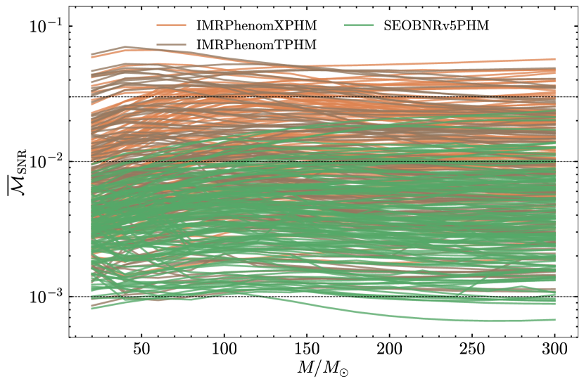
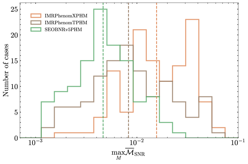
Figure 17: Left panel: Sky-averaged SNR weighted unfaithfulness as a function of the total mass of the system $[20,300]M_{\odot}$, of IMRPhenomXPHM (orange), IMRPhenomTPHM (brown) and SEOBNRv5PHM (green), against the 118 highly precessing simulations from Ref. [98]. Right panel: Distribution of the maximum unfaithfulness over the total mass range for each NR simulation considered in the left plot. The vertical dashed lines indicate the median values of the distribution.

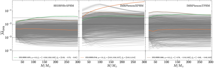
Figure 18: Sky-averaged SNR-weighted unfaithfulness as a function of the total mass of the system $[20,300]M_{\odot}$, of the SEOBNRv5PHM model (left panel), and the state-of-the-art phenomenological models, IMRPhenomXPHM (mid panel) and IMRPhenomTPHM (right panel), against 1543 precessing-spin SXS NR waveforms.

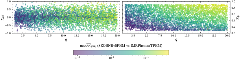
Figure 19: Maximum sky-and-polarization-averaged unfaithfulness weighted by the SNR over the total mass range $[20-300]M_{\odot}$ between SEOBNRv5PHM and IMRPhenomTPHM for 5000 random configurations with inclination $\iota_{s}=\pi/3$. The unfaithfulness grows with increasing mass ratio and spin magnitude values, and it can reach very large values for mass ratios $q\sim 20$ and $\chi_{\mathrm{p}}\sim 1$.

Considering the unfaithfulness against the 118 highly precessing NR waveforms from Ref. [98], we find in Fig. 17 a similar trend as in Fig. 4. The IMRPhenomTPHM model performs better than the IMRPhenomXPHM model, due to an improved description of the precessing-spin dynamics during the inspiral and merger-ringdown, however the lack of modeling effects due to the in-plane spin components in the waveform causes IMRPhenomTPHM to still have a significant number of cases with a maximum unfaithfulness above $3\%$ with respect to the SEOBNRv5PHM model. In particular, we find that the IMRPhenomTPHM model has $89\%$ $(58.5\%)$ of cases with a maximum unfaithfulness below $3\%$ $(1\%)$. These numbers reduce to $72.9\%$ $(24.6\%)$ for the IMRPhenomXPHM model, and they increase to $100\%$ $(85.6\%)$ for the SEOBNRv5PHM model. Therefore, when considering highly precessing-spin configurations the SEOBNRv5PHM model provides the lowest unfaithfulness, followed closely by the time-domain phenomenological IMRPhenomTPHM model, which offers an improved description of spin-precession with respect to the frequency-domain IMRPhenomXPHM model.

In Fig. 18 we turn to a comparison against a broader set of 1543 precessing-spin NR simulations. The IMRPhenomTPHM model reaches lower values of unfaithfulness than the SEOBNRv5PHM model for several configurations with low precessing-spin effects, which can be explained due to a slightly more accurate modeling of the higher order modes in the merger-ringdown in the aligned-spin limit (see Appendix G of Ref. [148] for details), but it also presents a significantly larger number of highly precessing configurations with unfaithfulness larger than $3\%$ with respect to the SEOBNRv5PHM model. Overall, the unfaithfulness of the IMRPhenomTPHM model is lower than the one of the IMRPhenomXPHM model. More quantitatively, we find that for IMRPhenomTPHM, $91.6\%$ $(62.4\%)$ of cases have a maximum unfaithfulness in the total mass range considered below $3\%$ $(1\%)$. These numbers reduce to $78.3\%$ $(38.3\%)$ for IMRPhenomXPHM, and increase to $99.8\%$ $(84.4\%)$ for SEOBNRv5PHM. Therefore, we find that the SEOBNRv5PHM model outperforms in accuracy the phenomenological models for highly precessing-spin configurations, while for low precessing configurations the accuracy of the models becomes more comparable, as they rely on the accuracy of the underlying non-precessing waveform models, which are calibrated to a similar set of non-precessing NR waveforms.

Finally, we repeat the study of Sec. IV.4 and compute the unfaithfulness between the SEOBNRv5PHM model as the template waveform and IMRPhenomTPHM as the signal, for 5000 configurations uniformly distributed in mass ratio $q\in[1,20]$ and effective spin parameter $\chi_{p}\in[0,0.99]$. Figure 19 shows the unfaithfulness as a function of mass ratio $q$, effective spin parameter $\chi_{\mathrm{eff}}$), and effective precessing-spin parameter $\chi_{\mathrm{p}}$. We find that for mass ratios $q<5$, there are $99.74\%$ ($64.5\%$) of cases with a maximum unfaithfulness, in total mass range $[20,300]M_{\odot}$, below $10\%$ $(1\%)$, while in Sec. IV.4 we found that for IMRPhenomXPHM these numbers decrease to $96.84\%$ ($41.3\%)$. The unfaithfulness increases significantly with mass ratio and spins, with the highest unfaithfulness values at the largest mass ratios $q\sim 20$, and effective spin precessing parameter $\chi_{\mathrm{p}}\sim 0.99$. In particular, when considering $q\leq 20$ we find that for IMRPhenomTPHM there are $73.84\%$ $(30.02\%)$ cases with maximum unfaithfulness, in the total mass range considered, below $10\%$ $(1\%)$, while these numbers increase to $59.19\%$ $(13.45\%)$ for IMRPhenomXPHM as shown in Sec. IV.4. The results show that the agreement of SEOBNRv5PHM with the time-domain model IMRPhenomTPHM is better than in the case of the frequency-domain phenomenological model IMRPhenomXPHM, due to the fact that the precessing-spin dynamics in IMRPhenomTPHM is more accurately described than in IMRPhenomXPHM. The existing large differences in unfaithfulness in some regions of the parameter space remark the necessity to populate this region with NR waveforms in order to reduce the systematics between models.

References

- Abbott et al. [2016] B. P. Abbott et al. (LIGO Scientific, Virgo), Phys. Rev. Lett. 116, 061102 (2016), arXiv:1602.03837 [gr-qc] .
- Abbott et al. [2019] B. P. Abbott et al. (LIGO Scientific, Virgo), Phys. Rev. X 9, 031040 (2019), arXiv:1811.12907 [astro-ph.HE] .
- Venumadhav et al. [2020] T. Venumadhav, B. Zackay, J. Roulet, L. Dai, and M. Zaldarriaga, Phys. Rev. D 101, 083030 (2020), arXiv:1904.07214 [astro-ph.HE] .
- Aasi et al. [2015] J. Aasi et al. (LIGO Scientific), Class. Quant. Grav. 32, 074001 (2015), arXiv:1411.4547 [gr-qc] .
- Acernese et al. [2015] F. Acernese et al. (VIRGO), Class. Quant. Grav. 32, 024001 (2015), arXiv:1408.3978 [gr-qc] .
- Abbott et al. [2021a] R. Abbott et al. (LIGO Scientific, Virgo), Phys. Rev. X 11, 021053 (2021a), arXiv:2010.14527 [gr-qc] .
- Abbott et al. [2021b] R. Abbott et al. (LIGO Scientific, VIRGO), (2021b), arXiv:2108.01045 [gr-qc] .
- Abbott et al. [2021c] R. Abbott et al. (LIGO Scientific, VIRGO, KAGRA), (2021c), arXiv:2111.03606 [gr-qc] .
- Nitz et al. [2021] A. H. Nitz, C. D. Capano, S. Kumar, Y.-F. Wang, S. Kastha, M. Schäfer, R. Dhurkunde, and M. Cabero, Astrophys. J. 922, 76 (2021), arXiv:2105.09151 [astro-ph.HE] .
- Olsen et al. [2022] S. Olsen, T. Venumadhav, J. Mushkin, J. Roulet, B. Zackay, and M. Zaldarriaga, Phys. Rev. D 106, 043009 (2022), arXiv:2201.02252 [astro-ph.HE] .
- Akutsu et al. [2019] T. Akutsu et al. (KAGRA), Nature Astron. 3, 35 (2019), arXiv:1811.08079 [gr-qc] .
- Akutsu et al. [2021] T. Akutsu et al. (KAGRA), PTEP 2021, 05A101 (2021), arXiv:2005.05574 [physics.ins-det] .
- Punturo et al. [2010] M. Punturo et al., Class. Quant. Grav. 27, 194002 (2010).
- Reitze et al. [2019] D. Reitze et al., Bull. Am. Astron. Soc. 51, 035 (2019), arXiv:1907.04833 [astro-ph.IM] .
- Evans et al. [2021] M. Evans et al., (2021), arXiv:2109.09882 [astro-ph.IM] .
- Amaro-Seoane et al. [2017] P. Amaro-Seoane, H. Audley, S. Babak, J. Baker, E. Barausse, P. Bender, E. Berti, P. Binetruy, M. Born, D. Bortoluzzi, et al., arXiv preprint arXiv:1702.00786 (2017).
- Apostolatos et al. [1994] T. A. Apostolatos, C. Cutler, G. J. Sussman, and K. S. Thorne, Phys. Rev. D 49, 6274 (1994).
- Blanchet [2014] L. Blanchet, Living Rev. Rel. 17, 2 (2014), arXiv:1310.1528 [gr-qc] .
- Rodriguez et al. [2016] C. L. Rodriguez, M. Zevin, C. Pankow, V. Kalogera, and F. A. Rasio, Astrophys. J. Lett. 832, L2 (2016), arXiv:1609.05916 [astro-ph.HE] .
- Stevenson et al. [2017] S. Stevenson, C. P. L. Berry, and I. Mandel, Mon. Not. Roy. Astron. Soc. 471, 2801 (2017), arXiv:1703.06873 [astro-ph.HE] .
- Talbot and Thrane [2017] C. Talbot and E. Thrane, Phys. Rev. D 96, 023012 (2017), arXiv:1704.08370 [astro-ph.HE] .
- Zhu et al. [2018] X. Zhu, E. Thrane, S. Oslowski, Y. Levin, and P. D. Lasky, Phys. Rev. D 98, 043002 (2018), arXiv:1711.09226 [astro-ph.HE] .
- Kimball et al. [2020] C. Kimball, C. Talbot, C. P. L. Berry, M. Carney, M. Zevin, E. Thrane, and V. Kalogera, Astrophys. J. 900, 177 (2020), arXiv:2005.00023 [astro-ph.HE] .
- Gompertz et al. [2022] B. P. Gompertz, M. Nicholl, P. Schmidt, G. Pratten, and A. Vecchio, Mon. Not. Roy. Astron. Soc. 511, 1454 (2022), arXiv:2108.10184 [astro-ph.HE] .
- Vecchio [2004] A. Vecchio, Phys. Rev. D 70, 042001 (2004), arXiv:astro-ph/0304051 .
- Lang and Hughes [2006] R. N. Lang and S. A. Hughes, Phys. Rev. D 74, 122001 (2006), [Erratum: Phys.Rev.D 75, 089902 (2007), Erratum: Phys.Rev.D 77, 109901 (2008)], arXiv:gr-qc/0608062 .
- Chatziioannou et al. [2015] K. Chatziioannou, N. Cornish, A. Klein, and N. Yunes, Astrophys. J. Lett. 798, L17 (2015), arXiv:1402.3581 [gr-qc] .
- Graff et al. [2015] P. B. Graff, A. Buonanno, and B. S. Sathyaprakash, Phys. Rev. D 92, 022002 (2015), arXiv:1504.04766 [gr-qc] .
- Pratten et al. [2020a] G. Pratten, P. Schmidt, R. Buscicchio, and L. M. Thomas, Phys. Rev. Res. 2, 043096 (2020a), arXiv:2006.16153 [gr-qc] .
- Johnson-McDaniel et al. [2022] N. K. Johnson-McDaniel, S. Kulkarni, and A. Gupta, Phys. Rev. D 106, 023001 (2022), arXiv:2107.11902 [astro-ph.HE] .
- Krishnendu and Ohme [2022] N. V. Krishnendu and F. Ohme, Phys. Rev. D 105, 064012 (2022), arXiv:2110.00766 [gr-qc] .
- Biscoveanu et al. [2021] S. Biscoveanu, M. Isi, V. Varma, and S. Vitale, Phys. Rev. D 104, 103018 (2021), arXiv:2106.06492 [gr-qc] .
- Steinle and Kesden [2022] N. Steinle and M. Kesden, Phys. Rev. D 106, 063028 (2022), arXiv:2206.00391 [astro-ph.HE] .
- Calderón Bustillo et al. [2021a] J. Calderón Bustillo, S. H. W. Leong, T. Dietrich, and P. D. Lasky, Astrophys. J. Lett. 912, L10 (2021a), arXiv:2006.11525 [gr-qc] .
- Ezquiaga [2021] J. M. Ezquiaga, Phys. Lett. B 822, 136665 (2021), arXiv:2104.05139 [astro-ph.CO] .
- Abbott et al. [2021d] R. Abbott et al. (LIGO Scientific, VIRGO, KAGRA), (2021d), arXiv:2111.03604 [astro-ph.CO] .
- Huwyler et al. [2012] C. Huwyler, A. Klein, and P. Jetzer, Phys. Rev. D 86, 084028 (2012), arXiv:1108.1826 [gr-qc] .
- Abbott et al. [2021e] R. Abbott et al. (LIGO Scientific, Virgo), Phys. Rev. D 103, 122002 (2021e), arXiv:2010.14529 [gr-qc] .
- Abbott et al. [2021f] R. Abbott et al. (LIGO Scientific, VIRGO, KAGRA), (2021f), arXiv:2112.06861 [gr-qc] .
- Pan et al. [2008] Y. Pan, A. Buonanno, J. G. Baker, J. Centrella, B. J. Kelly, S. T. McWilliams, F. Pretorius, and J. R. van Meter, Phys. Rev. D 77, 024014 (2008), arXiv:0704.1964 [gr-qc] .
- Ajith et al. [2007] P. Ajith et al., Class. Quant. Grav. 24, S689 (2007), arXiv:0704.3764 [gr-qc] .
- Ajith et al. [2011] P. Ajith et al., Phys. Rev. Lett. 106, 241101 (2011), arXiv:0909.2867 [gr-qc] .
- Santamaria et al. [2010] L. Santamaria et al., Phys. Rev. D 82, 064016 (2010), arXiv:1005.3306 [gr-qc] .
- Hannam et al. [2014] M. Hannam, P. Schmidt, A. Bohé, L. Haegel, S. Husa, F. Ohme, G. Pratten, and M. Pürrer, Phys. Rev. Lett. 113, 151101 (2014), arXiv:1308.3271 [gr-qc] .
- Husa et al. [2016] S. Husa, S. Khan, M. Hannam, M. Pürrer, F. Ohme, X. Jiménez Forteza, and A. Bohé, Phys. Rev. D 93, 044006 (2016), arXiv:1508.07250 [gr-qc] .
- Khan et al. [2016] S. Khan, S. Husa, M. Hannam, F. Ohme, M. Pürrer, X. Jiménez Forteza, and A. Bohé, Phys. Rev. D 93, 044007 (2016), arXiv:1508.07253 [gr-qc] .
- London et al. [2018] L. London, S. Khan, E. Fauchon-Jones, C. García, M. Hannam, S. Husa, X. Jiménez-Forteza, C. Kalaghatgi, F. Ohme, and F. Pannarale, Phys. Rev. Lett. 120, 161102 (2018), arXiv:1708.00404 [gr-qc] .
- Khan et al. [2019] S. Khan, K. Chatziioannou, M. Hannam, and F. Ohme, Phys. Rev. D 100, 024059 (2019), arXiv:1809.10113 [gr-qc] .
- Khan et al. [2020] S. Khan, F. Ohme, K. Chatziioannou, and M. Hannam, Phys. Rev. D 101, 024056 (2020), arXiv:1911.06050 [gr-qc] .
- Dietrich et al. [2019] T. Dietrich, A. Samajdar, S. Khan, N. K. Johnson-McDaniel, R. Dudi, and W. Tichy, Phys. Rev. D 100, 044003 (2019), arXiv:1905.06011 [gr-qc] .
- Pratten et al. [2020b] G. Pratten, S. Husa, C. Garcia-Quiros, M. Colleoni, A. Ramos-Buades, H. Estelles, and R. Jaume, Phys. Rev. D 102, 064001 (2020b), arXiv:2001.11412 [gr-qc] .
- Pratten et al. [2021] G. Pratten et al., Phys. Rev. D 103, 104056 (2021), arXiv:2004.06503 [gr-qc] .
- García-Quirós et al. [2020] C. García-Quirós, M. Colleoni, S. Husa, H. Estellés, G. Pratten, A. Ramos-Buades, M. Mateu-Lucena, and R. Jaume, Phys. Rev. D 102, 064002 (2020), arXiv:2001.10914 [gr-qc] .
- Estellés et al. [2021] H. Estellés, A. Ramos-Buades, S. Husa, C. García-Quirós, M. Colleoni, L. Haegel, and R. Jaume, Phys. Rev. D 103, 124060 (2021), arXiv:2004.08302 [gr-qc] .
- Estellés et al. [2022a] H. Estellés, S. Husa, M. Colleoni, D. Keitel, M. Mateu-Lucena, C. García-Quirós, A. Ramos-Buades, and A. Borchers, Phys. Rev. D 105, 084039 (2022a), arXiv:2012.11923 [gr-qc] .
- Estellés et al. [2022b] H. Estellés, M. Colleoni, C. García-Quirós, S. Husa, D. Keitel, M. Mateu-Lucena, M. d. L. Planas, and A. Ramos-Buades, Phys. Rev. D 105, 084040 (2022b), arXiv:2105.05872 [gr-qc] .
- Hamilton et al. [2021] E. Hamilton, L. London, J. E. Thompson, E. Fauchon-Jones, M. Hannam, C. Kalaghatgi, S. Khan, F. Pannarale, and A. Vano-Vinuales, Phys. Rev. D 104, 124027 (2021), arXiv:2107.08876 [gr-qc] .
- Blackman et al. [2015] J. Blackman, S. E. Field, C. R. Galley, B. Szilágyi, M. A. Scheel, M. Tiglio, and D. A. Hemberger, Phys. Rev. Lett. 115, 121102 (2015), arXiv:1502.07758 [gr-qc] .
- Blackman et al. [2017a] J. Blackman, S. E. Field, M. A. Scheel, C. R. Galley, D. A. Hemberger, P. Schmidt, and R. Smith, Phys. Rev. D 95, 104023 (2017a), arXiv:1701.00550 [gr-qc] .
- Blackman et al. [2017b] J. Blackman, S. E. Field, M. A. Scheel, C. R. Galley, C. D. Ott, M. Boyle, L. E. Kidder, H. P. Pfeiffer, and B. Szilágyi, Phys. Rev. D 96, 024058 (2017b), arXiv:1705.07089 [gr-qc] .
- Varma et al. [2019a] V. Varma, S. E. Field, M. A. Scheel, J. Blackman, L. E. Kidder, and H. P. Pfeiffer, Phys. Rev. D 99, 064045 (2019a), arXiv:1812.07865 [gr-qc] .
- Varma et al. [2019b] V. Varma, S. E. Field, M. A. Scheel, J. Blackman, D. Gerosa, L. C. Stein, L. E. Kidder, and H. P. Pfeiffer, Phys. Rev. Research. 1, 033015 (2019b), arXiv:1905.09300 [gr-qc] .
- Williams et al. [2020] D. Williams, I. S. Heng, J. Gair, J. A. Clark, and B. Khamesra, Phys. Rev. D 101, 063011 (2020), arXiv:1903.09204 [gr-qc] .
- Rifat et al. [2020] N. E. M. Rifat, S. E. Field, G. Khanna, and V. Varma, Phys. Rev. D 101, 081502 (2020), arXiv:1910.10473 [gr-qc] .
- Islam et al. [2021] T. Islam, V. Varma, J. Lodman, S. E. Field, G. Khanna, M. A. Scheel, H. P. Pfeiffer, D. Gerosa, and L. E. Kidder, Phys. Rev. D 103, 064022 (2021), arXiv:2101.11798 [gr-qc] .
- Islam et al. [2022] T. Islam, S. E. Field, S. A. Hughes, G. Khanna, V. Varma, M. Giesler, M. A. Scheel, L. E. Kidder, and H. P. Pfeiffer, Phys. Rev. D 106, 104025 (2022), arXiv:2204.01972 [gr-qc] .
- Yoo et al. [2022] J. Yoo, V. Varma, M. Giesler, M. A. Scheel, C.-J. Haster, H. P. Pfeiffer, L. E. Kidder, and M. Boyle, Phys. Rev. D 106, 044001 (2022), arXiv:2203.10109 [gr-qc] .
- Buonanno and Damour [1999] A. Buonanno and T. Damour, Phys. Rev. D 59, 084006 (1999), arXiv:gr-qc/9811091 .
- Buonanno and Damour [2000] A. Buonanno and T. Damour, Phys. Rev. D 62, 064015 (2000), arXiv:gr-qc/0001013 .
- Damour et al. [2000] T. Damour, P. Jaranowski, and G. Schaefer, Phys. Rev. D 62, 084011 (2000), arXiv:gr-qc/0005034 .
- Damour [2001] T. Damour, Phys. Rev. D 64, 124013 (2001), arXiv:gr-qc/0103018 .
- Buonanno et al. [2006] A. Buonanno, Y. Chen, and T. Damour, Phys. Rev. D 74, 104005 (2006), arXiv:gr-qc/0508067 .
- Buonanno et al. [2007a] A. Buonanno, G. B. Cook, and F. Pretorius, Phys. Rev. D 75, 124018 (2007a), arXiv:gr-qc/0610122 .
- Buonanno et al. [2007b] A. Buonanno, Y. Pan, J. G. Baker, J. Centrella, B. J. Kelly, S. T. McWilliams, and J. R. van Meter, Phys. Rev. D 76, 104049 (2007b), arXiv:0706.3732 [gr-qc] .
- Damour and Nagar [2008] T. Damour and A. Nagar, Phys. Rev. D 77, 024043 (2008), arXiv:0711.2628 [gr-qc] .
- Damour et al. [2009] T. Damour, B. R. Iyer, and A. Nagar, Phys. Rev. D 79, 064004 (2009), arXiv:0811.2069 [gr-qc] .
- Buonanno et al. [2009] A. Buonanno, Y. Pan, H. P. Pfeiffer, M. A. Scheel, L. T. Buchman, and L. E. Kidder, Phys. Rev. D 79, 124028 (2009), arXiv:0902.0790 [gr-qc] .
- Pan et al. [2011a] Y. Pan, A. Buonanno, M. Boyle, L. T. Buchman, L. E. Kidder, H. P. Pfeiffer, and M. A. Scheel, Phys. Rev. D 84, 124052 (2011a), arXiv:1106.1021 [gr-qc] .
- Damour et al. [2013] T. Damour, A. Nagar, and S. Bernuzzi, Phys. Rev. D 87, 084035 (2013), arXiv:1212.4357 [gr-qc] .
- Damour et al. [2015] T. Damour, P. Jaranowski, and G. Schäfer, Phys. Rev. D 91, 084024 (2015), arXiv:1502.07245 [gr-qc] .
- Nagar et al. [2020a] A. Nagar, G. Pratten, G. Riemenschneider, and R. Gamba, Phys. Rev. D 101, 024041 (2020a), arXiv:1904.09550 [gr-qc] .
- Damour et al. [2008a] T. Damour, A. Nagar, E. N. Dorband, D. Pollney, and L. Rezzolla, Phys. Rev. D 77, 084017 (2008a), arXiv:0712.3003 [gr-qc] .
- Damour et al. [2008b] T. Damour, P. Jaranowski, and G. Schaefer, Phys. Rev. D 78, 024009 (2008b), arXiv:0803.0915 [gr-qc] .
- Pan et al. [2010] Y. Pan, A. Buonanno, L. T. Buchman, T. Chu, L. E. Kidder, H. P. Pfeiffer, and M. A. Scheel, Phys. Rev. D 81, 084041 (2010), arXiv:0912.3466 [gr-qc] .
- Damour et al. [2008c] T. Damour, A. Nagar, M. Hannam, S. Husa, and B. Bruegmann, Phys. Rev. D 78, 044039 (2008c), arXiv:0803.3162 [gr-qc] .
- Barausse and Buonanno [2010] E. Barausse and A. Buonanno, Phys. Rev. D 81, 084024 (2010), arXiv:0912.3517 [gr-qc] .
- Barausse and Buonanno [2011] E. Barausse and A. Buonanno, Phys. Rev. D 84, 104027 (2011), arXiv:1107.2904 [gr-qc] .
- Nagar [2011] A. Nagar, Phys. Rev. D 84, 084028 (2011), [Erratum: Phys.Rev.D 88, 089901 (2013)], arXiv:1106.4349 [gr-qc] .
- Damour and Nagar [2014] T. Damour and A. Nagar, Phys. Rev. D 90, 044018 (2014), arXiv:1406.6913 [gr-qc] .
- Balmelli and Damour [2015] S. Balmelli and T. Damour, Phys. Rev. D 92, 124022 (2015), arXiv:1509.08135 [gr-qc] .
- Khalil et al. [2020] M. Khalil, J. Steinhoff, J. Vines, and A. Buonanno, Phys. Rev. D 101, 104034 (2020), arXiv:2003.04469 [gr-qc] .
- Taracchini et al. [2012] A. Taracchini, Y. Pan, A. Buonanno, E. Barausse, M. Boyle, T. Chu, G. Lovelace, H. P. Pfeiffer, and M. A. Scheel, Phys. Rev. D 86, 024011 (2012), arXiv:1202.0790 [gr-qc] .
- Taracchini et al. [2014a] A. Taracchini et al., Phys. Rev. D 89, 061502 (2014a), arXiv:1311.2544 [gr-qc] .
- Bohé et al. [2017] A. Bohé et al., Phys. Rev. D 95, 044028 (2017), arXiv:1611.03703 [gr-qc] .
- Cotesta et al. [2018] R. Cotesta, A. Buonanno, A. Bohé, A. Taracchini, I. Hinder, and S. Ossokine, Phys. Rev. D 98, 084028 (2018), arXiv:1803.10701 [gr-qc] .
- Pan et al. [2014] Y. Pan, A. Buonanno, A. Taracchini, L. E. Kidder, A. H. Mroué, H. P. Pfeiffer, M. A. Scheel, and B. Szilágyi, Phys. Rev. D 89, 084006 (2014), arXiv:1307.6232 [gr-qc] .
- Babak et al. [2017] S. Babak, A. Taracchini, and A. Buonanno, Phys. Rev. D 95, 024010 (2017), arXiv:1607.05661 [gr-qc] .
- Ossokine et al. [2020] S. Ossokine et al., Phys. Rev. D 102, 044055 (2020), arXiv:2004.09442 [gr-qc] .
- Nagar et al. [2019] A. Nagar, F. Messina, P. Rettegno, D. Bini, T. Damour, A. Geralico, S. Akcay, and S. Bernuzzi, Phys. Rev. D 99, 044007 (2019), arXiv:1812.07923 [gr-qc] .
- Nagar et al. [2018] A. Nagar et al., Phys. Rev. D 98, 104052 (2018), arXiv:1806.01772 [gr-qc] .
- Akcay et al. [2021] S. Akcay, R. Gamba, and S. Bernuzzi, Phys. Rev. D 103, 024014 (2021), arXiv:2005.05338 [gr-qc] .
- Gamba et al. [2022] R. Gamba, S. Akçay, S. Bernuzzi, and J. Williams, Phys. Rev. D 106, 024020 (2022), arXiv:2111.03675 [gr-qc] .
- Bini and Damour [2012] D. Bini and T. Damour, Phys. Rev. D 86, 124012 (2012), arXiv:1210.2834 [gr-qc] .
- Hinderer and Babak [2017] T. Hinderer and S. Babak, Phys. Rev. D 96, 104048 (2017), arXiv:1707.08426 [gr-qc] .
- Chiaramello and Nagar [2020] D. Chiaramello and A. Nagar, Phys. Rev. D 101, 101501 (2020), arXiv:2001.11736 [gr-qc] .
- Nagar et al. [2021] A. Nagar, A. Bonino, and P. Rettegno, Phys. Rev. D 103, 104021 (2021), arXiv:2101.08624 [gr-qc] .
- Khalil et al. [2021] M. Khalil, A. Buonanno, J. Steinhoff, and J. Vines, Phys. Rev. D 104, 024046 (2021), arXiv:2104.11705 [gr-qc] .
- Ramos-Buades et al. [2022] A. Ramos-Buades, A. Buonanno, M. Khalil, and S. Ossokine, Phys. Rev. D 105, 044035 (2022), arXiv:2112.06952 [gr-qc] .
- Albanesi et al. [2022] S. Albanesi, A. Placidi, A. Nagar, M. Orselli, and S. Bernuzzi, Phys. Rev. D 105, L121503 (2022), arXiv:2203.16286 [gr-qc] .
- Bernuzzi et al. [2015] S. Bernuzzi, A. Nagar, T. Dietrich, and T. Damour, Phys. Rev. Lett. 114, 161103 (2015), arXiv:1412.4553 [gr-qc] .
- Hinderer et al. [2016] T. Hinderer et al., Phys. Rev. Lett. 116, 181101 (2016), arXiv:1602.00599 [gr-qc] .
- Steinhoff et al. [2016] J. Steinhoff, T. Hinderer, A. Buonanno, and A. Taracchini, Phys. Rev. D 94, 104028 (2016), arXiv:1608.01907 [gr-qc] .
- Akcay et al. [2019] S. Akcay, S. Bernuzzi, F. Messina, A. Nagar, N. Ortiz, and P. Rettegno, Phys. Rev. D 99, 044051 (2019), arXiv:1812.02744 [gr-qc] .
- Steinhoff et al. [2021] J. Steinhoff, T. Hinderer, T. Dietrich, and F. Foucart, Phys. Rev. Res. 3, 033129 (2021), arXiv:2103.06100 [gr-qc] .
- Matas et al. [2020] A. Matas et al., Phys. Rev. D 102, 043023 (2020), arXiv:2004.10001 [gr-qc] .
- Gonzalez et al. [2022] A. Gonzalez, R. Gamba, M. Breschi, F. Zappa, G. Carullo, S. Bernuzzi, and A. Nagar, (2022), arXiv:2212.03909 [gr-qc] .
- Damour [2016] T. Damour, Phys. Rev. D 94, 104015 (2016), arXiv:1609.00354 [gr-qc] .
- Damour [2018] T. Damour, Phys. Rev. D 97, 044038 (2018), arXiv:1710.10599 [gr-qc] .
- Antonelli et al. [2019] A. Antonelli, A. Buonanno, J. Steinhoff, M. van de Meent, and J. Vines, Phys. Rev. D 99, 104004 (2019), arXiv:1901.07102 [gr-qc] .
- Damgaard and Vanhove [2021] P. H. Damgaard and P. Vanhove, Phys. Rev. D 104, 104029 (2021), arXiv:2108.11248 [hep-th] .
- Khalil et al. [2022] M. Khalil, A. Buonanno, J. Steinhoff, and J. Vines, Phys. Rev. D 106, 024042 (2022), arXiv:2204.05047 [gr-qc] .
- Damour and Rettegno [2022] T. Damour and P. Rettegno, (2022), arXiv:2211.01399 [gr-qc] .
- Damour [2010] T. Damour, Phys. Rev. D 81, 024017 (2010), arXiv:0910.5533 [gr-qc] .
- Yunes et al. [2010] N. Yunes, A. Buonanno, S. A. Hughes, M. Coleman Miller, and Y. Pan, Phys. Rev. Lett. 104, 091102 (2010), arXiv:0909.4263 [gr-qc] .
- Yunes et al. [2011] N. Yunes, A. Buonanno, S. A. Hughes, Y. Pan, E. Barausse, M. C. Miller, and W. Throwe, Phys. Rev. D 83, 044044 (2011), [Erratum: Phys.Rev.D 88, 109904 (2013)], arXiv:1009.6013 [gr-qc] .
- Barausse et al. [2012a] E. Barausse, A. Buonanno, and A. Le Tiec, Phys. Rev. D 85, 064010 (2012a), arXiv:1111.5610 [gr-qc] .
- Akcay et al. [2012] S. Akcay, L. Barack, T. Damour, and N. Sago, Phys. Rev. D 86, 104041 (2012), arXiv:1209.0964 [gr-qc] .
- Antonelli et al. [2020] A. Antonelli, M. van de Meent, A. Buonanno, J. Steinhoff, and J. Vines, Phys. Rev. D 101, 024024 (2020), arXiv:1907.11597 [gr-qc] .
- Nagar and Albanesi [2022] A. Nagar and S. Albanesi, Phys. Rev. D 106, 064049 (2022), arXiv:2207.14002 [gr-qc] .
- Field et al. [2014] S. E. Field, C. R. Galley, J. S. Hesthaven, J. Kaye, and M. Tiglio, Phys. Rev. X 4, 031006 (2014), arXiv:1308.3565 [gr-qc] .
- Pürrer [2014] M. Pürrer, Class. Quant. Grav. 31, 195010 (2014), arXiv:1402.4146 [gr-qc] .
- Pürrer [2016] M. Pürrer, Phys. Rev. D 93, 064041 (2016), arXiv:1512.02248 [gr-qc] .
- Lackey et al. [2017] B. D. Lackey, S. Bernuzzi, C. R. Galley, J. Meidam, and C. Van Den Broeck, Phys. Rev. D 95, 104036 (2017), arXiv:1610.04742 [gr-qc] .
- Lackey et al. [2019] B. D. Lackey, M. Pürrer, A. Taracchini, and S. Marsat, Phys. Rev. D 100, 024002 (2019), arXiv:1812.08643 [gr-qc] .
- Cotesta et al. [2020] R. Cotesta, S. Marsat, and M. Pürrer, Phys. Rev. D 101, 124040 (2020), arXiv:2003.12079 [gr-qc] .
- Gadre et al. [2022] B. Gadre, M. Pürrer, S. E. Field, S. Ossokine, and V. Varma, (2022), arXiv:2203.00381 [gr-qc] .
- Tissino et al. [2022] J. Tissino, G. Carullo, M. Breschi, R. Gamba, S. Schmidt, and S. Bernuzzi, (2022), arXiv:2210.15684 [gr-qc] .
- Khan and Green [2021] S. Khan and R. Green, Phys. Rev. D 103, 064015 (2021), arXiv:2008.12932 [gr-qc] .
- Thomas et al. [2022] L. M. Thomas, G. Pratten, and P. Schmidt, Phys. Rev. D 106, 104029 (2022), arXiv:2205.14066 [gr-qc] .
- Nagar et al. [2020b] A. Nagar, G. Riemenschneider, G. Pratten, P. Rettegno, and F. Messina, Phys. Rev. D 102, 024077 (2020b), arXiv:2001.09082 [gr-qc] .
- Buonanno et al. [2003] A. Buonanno, Y.-b. Chen, and M. Vallisneri, Phys. Rev. D 67, 104025 (2003), [Erratum: Phys.Rev.D 74, 029904 (2006)], arXiv:gr-qc/0211087 .
- Schmidt et al. [2011] P. Schmidt, M. Hannam, S. Husa, and P. Ajith, Phys. Rev. D 84, 024046 (2011), arXiv:1012.2879 [gr-qc] .
- Boyle et al. [2011] M. Boyle, R. Owen, and H. P. Pfeiffer, Phys. Rev. D 84, 124011 (2011), arXiv:1110.2965 [gr-qc] .
- O’Shaughnessy et al. [2011] R. O’Shaughnessy, B. Vaishnav, J. Healy, Z. Meeks, and D. Shoemaker, Phys. Rev. D 84, 124002 (2011), arXiv:1109.5224 [gr-qc] .
- Schmidt et al. [2012] P. Schmidt, M. Hannam, and S. Husa, Phys. Rev. D 86, 104063 (2012), arXiv:1207.3088 [gr-qc] .
- [146] R. Sturani, Note on the derivation of the angular momentum and spin precessing equations in spintaylor codes, https://dcc.ligo.org/public/0122/T1500554/023/dLdS.pdf.
- Khalil et al. [2023] M. Khalil, A. Buonanno, H. Estellés, D. Mihaylov, S. Ossokine, L. Pompili, and A. Ramos-Buades, (2023).
- Pompili et al. [2023] L. Pompili, A. Buonanno, H. Estellés, M. Khalil, M. van de Meent, D. Mihaylov, S. Ossokine, M. Pürrer, A. Ramos-Buades, A. Kumar Mehta, R. Cotesta, S. Marsat, M. Boyle, L. E. Kidder, H. P. Pfeiffer, M. A. Scheel, H. R. Rüter, N. Vu, R. Dudi, S. Ma, K. Mitman, D. Melchor, S. Thomas, and J. Sanchez, (2023).
- Mroue et al. [2013] A. H. Mroue et al., Phys. Rev. Lett. 111, 241104 (2013), arXiv:1304.6077 [gr-qc] .
- Boyle et al. [2019] M. Boyle et al., Class. Quant. Grav. 36, 195006 (2019), arXiv:1904.04831 [gr-qc] .
- Barausse et al. [2012b] E. Barausse, A. Buonanno, S. A. Hughes, G. Khanna, S. O’Sullivan, and Y. Pan, Phys. Rev. D 85, 024046 (2012b), arXiv:1110.3081 [gr-qc] .
- Taracchini et al. [2014b] A. Taracchini, A. Buonanno, G. Khanna, and S. A. Hughes, Phys. Rev. D 90, 084025 (2014b), arXiv:1404.1819 [gr-qc] .
- van de Meent et al. [2023] M. van de Meent, A. Buonanno, D. Mihaylov, S. Ossokine, L. Pompili, N. Warburton, A. Pound, B. Wardell, L. Durkan, and J. Miller, (2023).
- Warburton et al. [2021] N. Warburton, A. Pound, B. Wardell, J. Miller, and L. Durkan, Phys. Rev. Lett. 127, 151102 (2021), arXiv:2107.01298 [gr-qc] .
- Wardell et al. [2021] B. Wardell, A. Pound, N. Warburton, J. Miller, L. Durkan, and A. Le Tiec, (2021), arXiv:2112.12265 [gr-qc] .
- Gonzalez et al. [2009] J. A. Gonzalez, U. Sperhake, and B. Bruegmann, Phys. Rev. D 79, 124006 (2009), arXiv:0811.3952 [gr-qc] .
- Buchman et al. [2012] L. T. Buchman, H. P. Pfeiffer, M. A. Scheel, and B. Szilagyi, Phys. Rev. D 86, 084033 (2012), arXiv:1206.3015 [gr-qc] .
- Chu et al. [2009] T. Chu, H. P. Pfeiffer, and M. A. Scheel, Phys. Rev. D 80, 124051 (2009), arXiv:0909.1313 [gr-qc] .
- Jani et al. [2016] K. Jani, J. Healy, J. A. Clark, L. London, P. Laguna, and D. Shoemaker, Class. Quant. Grav. 33, 204001 (2016), arXiv:1605.03204 [gr-qc] .
- Foucart et al. [2019] F. Foucart et al., Phys. Rev. D 99, 044008 (2019), arXiv:1812.06988 [gr-qc] .
- Healy et al. [2017] J. Healy, C. O. Lousto, Y. Zlochower, and M. Campanelli, Class. Quant. Grav. 34, 224001 (2017), arXiv:1703.03423 [gr-qc] .
- Hinder et al. [2019] I. Hinder, S. Ossokine, H. P. Pfeiffer, and A. Buonanno, Phys. Rev. D 99, 061501 (2019), arXiv:1810.10585 [gr-qc] .
- Healy et al. [2019] J. Healy, C. O. Lousto, J. Lange, R. O’Shaughnessy, Y. Zlochower, and M. Campanelli, Phys. Rev. D 100, 024021 (2019), arXiv:1901.02553 [gr-qc] .
- Healy and Lousto [2022] J. Healy and C. O. Lousto, Phys. Rev. D 105, 124010 (2022), arXiv:2202.00018 [gr-qc] .
- Nagar and Rettegno [2019] A. Nagar and P. Rettegno, Phys. Rev. D 99, 021501 (2019), arXiv:1805.03891 [gr-qc] .
- Rettegno et al. [2020] P. Rettegno, F. Martinetti, A. Nagar, D. Bini, G. Riemenschneider, and T. Damour, Phys. Rev. D 101, 104027 (2020), arXiv:1911.10818 [gr-qc] .
- Mihaylov et al. [2021] D. P. Mihaylov, S. Ossokine, A. Buonanno, and A. Ghosh, Phys. Rev. D 104, 124087 (2021), arXiv:2105.06983 [gr-qc] .
- Mihaylov et al. [2023] D. Mihaylov, S. Ossokine, A. Buonanno, H. Estellés, L. Pompili, M. Pürrer, and A. Ramos-Buades, (2023).
- Pankow et al. [2015] C. Pankow, P. Brady, E. Ochsner, and R. O’Shaughnessy, Phys. Rev. D 92, 023002 (2015), arXiv:1502.04370 [gr-qc] .
- Lange et al. [2018] J. Lange, R. O’Shaughnessy, and M. Rizzo, (2018), arXiv:1805.10457 [gr-qc] .
- Green and Gair [2021] S. R. Green and J. Gair, Mach. Learn. Sci. Tech. 2, 03LT01 (2021), arXiv:2008.03312 [astro-ph.IM] .
- Dax et al. [2021] M. Dax, S. R. Green, J. Gair, J. H. Macke, A. Buonanno, and B. Schölkopf, Phys. Rev. Lett. 127, 241103 (2021), arXiv:2106.12594 [gr-qc] .
- Dax et al. [2022] M. Dax, S. R. Green, J. Gair, M. Pürrer, J. Wildberger, J. H. Macke, A. Buonanno, and B. Schölkopf, (2022), arXiv:2210.05686 [gr-qc] .
- Sathyaprakash and Schutz [2009] B. S. Sathyaprakash and B. F. Schutz, Living Rev. Rel. 12, 2 (2009), arXiv:0903.0338 [gr-qc] .
- Racine [2008] E. Racine, Phys. Rev. D 78, 044021 (2008), arXiv:0803.1820 [gr-qc] .
- Schmidt et al. [2015] P. Schmidt, F. Ohme, and M. Hannam, Phys. Rev. D 91, 024043 (2015), arXiv:1408.1810 [gr-qc] .
- Damour and Nagar [2007] T. Damour and A. Nagar, Phys. Rev. D 76, 064028 (2007), arXiv:0705.2519 [gr-qc] .
- Knowles et al. [2018] T. D. Knowles, C. Devine, D. A. Buch, S. A. Bilgili, T. R. Adams, Z. B. Etienne, and S. T. Mcwilliams, Class. Quant. Grav. 35, 155003 (2018), arXiv:1803.06346 [gr-qc] .
- Bohé et al. [2015] A. Bohé, G. Faye, S. Marsat, and E. K. Porter, Class. Quant. Grav. 32, 195010 (2015), arXiv:1501.01529 [gr-qc] .
- Cho et al. [2022] G. Cho, R. A. Porto, and Z. Yang, (2022), arXiv:2201.05138 [gr-qc] .
- Chatziioannou et al. [2013] K. Chatziioannou, A. Klein, N. Yunes, and N. Cornish, Phys. Rev. D 88, 063011 (2013), arXiv:1307.4418 [gr-qc] .
- Pan et al. [2011b] Y. Pan, A. Buonanno, R. Fujita, E. Racine, and H. Tagoshi, Phys. Rev. D 83, 064003 (2011b), [Erratum: Phys.Rev.D 87, 109901 (2013)], arXiv:1006.0431 [gr-qc] .
- Arun et al. [2009] K. G. Arun, A. Buonanno, G. Faye, and E. Ochsner, Phys. Rev. D 79, 104023 (2009), [Erratum: Phys.Rev.D 84, 049901 (2011)], arXiv:0810.5336 [gr-qc] .
- Mishra et al. [2016] C. K. Mishra, A. Kela, K. G. Arun, and G. Faye, Phys. Rev. D 93, 084054 (2016), arXiv:1601.05588 [gr-qc] .
- Taracchini et al. [2013] A. Taracchini, A. Buonanno, S. A. Hughes, and G. Khanna, Phys. Rev. D 88, 044001 (2013), [Erratum: Phys.Rev.D 88, 109903 (2013)], arXiv:1305.2184 [gr-qc] .
- Bernuzzi et al. [2011] S. Bernuzzi, A. Nagar, and A. Zenginoglu, Phys. Rev. D 84, 084026 (2011), arXiv:1107.5402 [gr-qc] .
- Harms et al. [2016] E. Harms, G. Lukes-Gerakopoulos, S. Bernuzzi, and A. Nagar, Phys. Rev. D 93, 044015 (2016), [Addendum: Phys.Rev.D 100, 129901 (2019)], arXiv:1510.05548 [gr-qc] .
- Boyle et al. [2022] M. Boyle, J. Long, M. Ling, stiiin, B. Bonnett, L. C. Stein, E. Wieser, D. A. B. Iozzo, H. Haglid, J. Belmonte, J. Long, M. Wiebe, Y. Li, Z. Vinícius, J. Macfarlane, and odidev, moble/quaternion: Release v2022.4.2 (2022).
- Boyle [2013] M. Boyle, Phys. Rev. D 87, 104006 (2013), arXiv:1302.2919 [gr-qc] .
- Boyle et al. [2014] M. Boyle, L. E. Kidder, S. Ossokine, and H. P. Pfeiffer, (2014), arXiv:1409.4431 [gr-qc] .
- Boyle [2016] M. Boyle, Phys. Rev. D 93, 084031 (2016), arXiv:1509.00862 [gr-qc] .
- Berti et al. [2006] E. Berti, V. Cardoso, and C. M. Will, Phys. Rev. D 73, 064030 (2006), arXiv:gr-qc/0512160 .
- O’Shaughnessy et al. [2013] R. O’Shaughnessy, L. London, J. Healy, and D. Shoemaker, Phys. Rev. D 87, 044038 (2013), arXiv:1209.3712 [gr-qc] .
- Hamilton et al. [2023] E. Hamilton, L. London, and M. Hannam, (2023), arXiv:2301.06558 [gr-qc] .
- Varma et al. [2019c] V. Varma, D. Gerosa, L. C. Stein, F. Hébert, and H. Zhang, Phys. Rev. Lett. 122, 011101 (2019c), arXiv:1809.09125 [gr-qc] .
- Jiménez-Forteza et al. [2017] X. Jiménez-Forteza, D. Keitel, S. Husa, M. Hannam, S. Khan, and M. Pürrer, Phys. Rev. D 95, 064024 (2017), arXiv:1611.00332 [gr-qc] .
- Hofmann et al. [2016] F. Hofmann, E. Barausse, and L. Rezzolla, Astrophys. J. Lett. 825, L19 (2016), arXiv:1605.01938 [gr-qc] .
- Sathyaprakash and Dhurandhar [1991] B. S. Sathyaprakash and S. V. Dhurandhar, Phys. Rev. D 44, 3819 (1991).
- Finn and Chernoff [1993] L. S. Finn and D. F. Chernoff, Phys. Rev. D 47, 2198 (1993), arXiv:gr-qc/9301003 .
- Barsotti et al. [2018] L. Barsotti, P. Fritschel, M. Evans, and S. Gras (LIGO Collaboration), Updated advanced ligo sensitivity design curve (2018), LIGO Document T1800044-v5.
- Capano et al. [2014] C. Capano, Y. Pan, and A. Buonanno, Phys. Rev. D 89, 102003 (2014), arXiv:1311.1286 [gr-qc] .
- Gamba et al. [2023] R. Gamba, M. Breschi, G. Carullo, S. Albanesi, P. Rettegno, S. Bernuzzi, and A. Nagar, Nature Astron. 7, 11 (2023), arXiv:2106.05575 [gr-qc] .
- [203] https://www.black-holes.org/SpEC.html.
- Ashton and Talbot [2021] G. Ashton and C. Talbot, Mon. Not. Roy. Astron. Soc. 507, 2037 (2021), arXiv:2106.08730 [gr-qc] .
- Williams et al. [2021] M. J. Williams, J. Veitch, and C. Messenger, Phys. Rev. D 103, 103006 (2021), arXiv:2102.11056 [gr-qc] .
- Williams et al. [2023] M. J. Williams, J. Veitch, and C. Messenger, (2023), arXiv:2302.08526 [astro-ph.IM] .
- LIGO Scientific Collaboration [2018] LIGO Scientific Collaboration, LIGO Algorithm Library - LALSuite, free software (GPL) (2018).
- Smith et al. [2020] R. J. E. Smith, G. Ashton, A. Vajpeyi, and C. Talbot, Mon. Not. Roy. Astron. Soc. 498, 4492 (2020), arXiv:1909.11873 [gr-qc] .
- Ashton et al. [2019] G. Ashton et al., Astrophys. J. Suppl. 241, 27 (2019), arXiv:1811.02042 [astro-ph.IM] .
- Romero-Shaw et al. [2020a] I. M. Romero-Shaw et al., Mon. Not. Roy. Astron. Soc. 499, 3295 (2020a), arXiv:2006.00714 [astro-ph.IM] .
- Callister [2021] T. Callister, (2021), arXiv:2104.09508 [gr-qc] .
- Abbott et al. [2021g] R. Abbott et al. (LIGO Scientific, Virgo), SoftwareX 13, 100658 (2021g), arXiv:1912.11716 [gr-qc] .
- Speagle [2020] J. S. Speagle, Mon. Not. Roy. Astron. Soc. 493, 3132 (2020), arXiv:1904.02180 [astro-ph.IM] .
- Abbott et al. [2020] R. Abbott et al. (LIGO Scientific, Virgo), Phys. Rev. D 102, 043015 (2020), arXiv:2004.08342 [astro-ph.HE] .
- Colleoni et al. [2021] M. Colleoni, M. Mateu-Lucena, H. Estellés, C. García-Quirós, D. Keitel, G. Pratten, A. Ramos-Buades, and S. Husa, Phys. Rev. D 103, 024029 (2021), arXiv:2010.05830 [gr-qc] .
- Gayathri et al. [2022] V. Gayathri, J. Healy, J. Lange, B. O’Brien, M. Szczepanczyk, I. Bartos, M. Campanelli, S. Klimenko, C. O. Lousto, and R. O’Shaughnessy, Nature Astron. 6, 344 (2022), arXiv:2009.05461 [astro-ph.HE] .
- Romero-Shaw et al. [2020b] I. M. Romero-Shaw, P. D. Lasky, E. Thrane, and J. C. Bustillo, Astrophys. J. Lett. 903, L5 (2020b), arXiv:2009.04771 [astro-ph.HE] .
- Calderón Bustillo et al. [2021b] J. Calderón Bustillo, N. Sanchis-Gual, A. Torres-Forné, J. A. Font, A. Vajpeyi, R. Smith, C. Herdeiro, E. Radu, and S. H. W. Leong, Phys. Rev. Lett. 126, 081101 (2021b), arXiv:2009.05376 [gr-qc] .
- Estellés et al. [2022c] H. Estellés et al., Astrophys. J. 924, 79 (2022c), arXiv:2105.06360 [gr-qc] .
- Veitch et al. [2015] J. Veitch et al., Phys. Rev. D 91, 042003 (2015), arXiv:1409.7215 [gr-qc] .
- Hannam et al. [2022] M. Hannam et al., Nature 610, 652 (2022), arXiv:2112.11300 [gr-qc] .
- Payne et al. [2022] E. Payne, S. Hourihane, J. Golomb, R. Udall, R. Udall, D. Davis, and K. Chatziioannou, Phys. Rev. D 106, 104017 (2022), arXiv:2206.11932 [gr-qc] .
- Balmelli and Jetzer [2015] S. Balmelli and P. Jetzer, Phys. Rev. D 91, 064011 (2015), arXiv:1502.01343 [gr-qc] .
- Henry [2022] Q. Henry, (2022), arXiv:2210.15602 [gr-qc] .
- Henry et al. [2022] Q. Henry, S. Marsat, and M. Khalil, Phys. Rev. D 106, 124018 (2022), arXiv:2209.00374 [gr-qc] .
- Pound et al. [2020] A. Pound, B. Wardell, N. Warburton, and J. Miller, Phys. Rev. Lett. 124, 021101 (2020), arXiv:1908.07419 [gr-qc] .
- Estelles et al. [2023] H. Estelles et al., in preparation (2023).
- Ghosh et al. [2021] A. Ghosh, R. Brito, and A. Buonanno, Phys. Rev. D 103, 124041 (2021), arXiv:2104.01906 [gr-qc] .
- Mehta et al. [2023] A. K. Mehta, A. Buonanno, R. Cotesta, A. Ghosh, N. Sennett, and J. Steinhoff, Phys. Rev. D 107, 044020 (2023), arXiv:2203.13937 [gr-qc] .
- Maggio et al. [2022] E. Maggio, H. O. Silva, A. Buonanno, and A. Ghosh, (2022), arXiv:2212.09655 [gr-qc] .
- Okounkova et al. [2020] M. Okounkova, L. C. Stein, J. Moxon, M. A. Scheel, and S. A. Teukolsky, Phys. Rev. D 101, 104016 (2020), arXiv:1911.02588 [gr-qc] .
- Okounkova et al. [2019] M. Okounkova, L. C. Stein, M. A. Scheel, and S. A. Teukolsky, Phys. Rev. D 100, 104026 (2019), arXiv:1906.08789 [gr-qc] .
- Silva et al. [2021] H. O. Silva, H. Witek, M. Elley, and N. Yunes, Phys. Rev. Lett. 127, 031101 (2021), arXiv:2012.10436 [gr-qc] .
- Okounkova et al. [2023] M. Okounkova, M. Isi, K. Chatziioannou, and W. M. Farr, Phys. Rev. D 107, 024046 (2023), arXiv:2208.02805 [gr-qc] .
- Corman et al. [2023] M. Corman, J. L. Ripley, and W. E. East, Phys. Rev. D 107, 024014 (2023), arXiv:2210.09235 [gr-qc] .