Simple Domain Generalization Methods are Strong Baselines
for Open Domain Generalization

Abstract

In real-world applications, a machine learning model is required to handle an open-set recognition (OSR), where unknown classes appear during the inference, in addition to a domain shift, where the distribution of data differs between the training and inference phases. Domain generalization (DG) aims to handle the domain shift situation where the target domain of the inference phase is inaccessible during model training. Open domain generalization (ODG) takes into account both DG and OSR. Domain-Augmented Meta-Learning (DAML) is a method targeting ODG but has a complicated learning process. On the other hand, although various DG methods have been proposed, they have not been evaluated in ODG situations. This work comprehensively evaluates existing DG methods in ODG and shows that two simple DG methods, CORrelation ALignment (CORAL) and Maximum Mean Discrepancy (MMD), are competitive with DAML in several cases. In addition, we propose simple extensions of CORAL and MMD by introducing the techniques used in DAML, such as ensemble learning and Dirichlet mixup data augmentation. The experimental evaluation demonstrates that the extended CORAL and MMD can perform comparably to DAML with lower computational costs. This suggests that the simple DG methods and their simple extensions are strong baselines for ODG. The code used in the experiments is available at https://github.com/shiralab/OpenDG-Eval.

1 Introduction

Machine learning has significantly succeeded in various fields, such as image and speech recognition and natural language processing [26]. However, it is known that the performance of machine learning models degrades significantly in situations where data distribution differs between the training and inference (testing) phases [10]. This situation is called domain shift and often appears in real-world machine learning applications [21], including computer vision tasks. We call the domains (i.e., the data distribution or characteristics) that can be accessed in model training the source domains. In contrast, the domains in the testing phase are called target domains. Domain generalization (DG) [30, 33] is an approach to address the domain shift. DG methods only use the source domain data during the training phase and do not use the target domain data.

Open-set recognition (OSR) [6, 17] is another requirement in real-world applications of classification models. Although the class space, i.e., the number and contents of classes, is identical between the training and testing phases in the usual machine learning and DG situations, OSR deals with the situation where the source and target class spaces are not the same. The objective of the OSR methods is to detect unknown classes while correctly recognizing known classes in the testing phase. Most OSR methods do not take into account the domain shift between the training and testing phases.

The situation considering both DG and OSR is called open domain generalization (ODG), which was introduced in [24]. While ODG is also frequently encountered in real-world applications, such as autonomous driving and medical assistance, methods for ODG have not been fully developed. Domain-augmented meta-learning (DAML) [24] is a state-of-the-art method to address ODG, but it has a complicated learning process and consists of several training components.

The work of [8] shows that the carefully implemented and tuned simple empirical risk minimization (ERM) method without any specific technique for DG outperforms many state-of-the-art DG methods. Furthermore, in OSR, ERM with several simple modifications, such as data augmentation, label smoothing, and using logits rather than softmax probabilities, has exhibited comparable performance with more complex state-of-the-art OSR methods [28]. The lesson from these studies is the importance of comprehensively evaluating simple baseline methods rather than developing complicated ones. In general, simple methods are advantageous regarding computational cost, implementation, and ease of combining other techniques.

Because existing DG methods have not been thoroughly evaluated in ODG situations, we first comprehensively evaluate the existing DG method in ODG situations. We show that simple DG methods, CORrelation ALignment (CORAL) [25] and maximum mean discrepancy (MMD) [7], perform better than other DG methods and are comparable to state-of-the-art DAML on datasets where the effectiveness of data augmentation is low. Because CORAL and MMD are simple and easy to combine with other enhanced training methods, we propose introducing the techniques used in DAML, ensemble learning, Dirichlet mixup (Dir-mixup) data augmentation, and knowledge distillation, into CORAL and MMD to improve their performances. The experimental result demonstrates that CORAL and MMD with Dir-mixup data augmentation achieve comparable performances with DAML on datasets where data augmentation is effective. The contributions of this paper are as follows.

• We comprehensively evaluate the DG methods in ODG.

• We propose the extended methods of CORAL and MMD by injecting the techniques used in DAML.

• Empirical evaluation reveals that simple DG methods and their extensions can be strong baselines for ODG, which would be useful for practitioners and further algorithm developments.

2 Key Algorithms

This section describes the methods focussed in the paper.

2.1 CORAL and MMD

CORAL [25] and MMD [15] are the classic DG methods, which introduce the additional term in the loss function.

CORAL uses the loss of $\ell_{CORAL}$, which is the sum of the difference in the covariance matrices $C_{i}$ and $C_{j}$ of the features for each source domain. The loss $\ell_{CORAL}$ is given by

$$\ell_{CORAL}=\frac{1}{M^{2}}\sum_{1\leq i\leq M}\sum_{1\leq j\leq M}\left\|C_{i}-C_{j}\right\|_{F}^{2}\enspace,$$ (1)

where $M$ is the number of source domains, $C_{i}$ represents the covariance matrix of features for the $i$-th domain, and $\|\cdot\|_{F}$ is the Frobenius norm.

MMD [15] measures the distance between the training data distributions of $P^{i}_{X}$ and $P^{j}_{X}$ by the maximum mean discrepancy [7]. The loss $\ell_{MMD}$ in our domain generalization scenario is defined by

$$\ell_{MMD}=\frac{1}{M^{2}}\sum_{1\leq i\leq M}\sum_{1\leq j\leq M}\text{MMD}(P^{i}_{X},P^{j}_{X})^{2}\enspace,$$ (2)

where $\text{MMD}(P^{i}_{X},P^{j}_{X})$ measures the distance between the feature distributions of the $i$- and $j$-th domains.

In model training, the cross entropy loss with $\ell_{CORAL}$ or $\ell_{MMD}$ is minimized, and the covariance matrix $C_{i}$ in CORAL and the MMD function are calculated using mini-batch samples.

2.2 Domain-augmented meta-learning (DAML)

2.2.1 Open Domain Generalization (ODG)

ODG [24] is a task combined with DG and OSR. In ODG, the target domain is inaccessible during training and may differ from the source domains. In addition, the class spaces of the source and target domains are different, and unknown classes appear in the target domain. A similar scenario in which input data in target domains are accessible is called open domain adaptation (ODA) [23], a combination of domain adaptation and OSR. ODA is a more realistic problem than general domain adaptation, but it assumes that target data are available during the training phase while they are inaccessible in ODG.

The literature on DAML [24] assumed that multiple source domains are accessible during training. Although a method for open-set single-domain generalization with a single domain in training has recently been proposed [34, 31], this study focuses on ODG with multiple source domains for training as in [24]. Note that, to our knowledge, DAML is the only method proposed for ODG with multiple source domains. In [24], several DG methods are evaluated in ODG as baselines. However, classic and simple DG methods, such as CORAL and MMD, have not been comprehensively evaluated in ODG.

2.2.2 Algorithm of DAML

DAML is an ensemble method that prepares the same number of models as source domains for training. Each model is trained in two stages by meta-learning using Dir-mixup data augmentation and knowledge distillation.

Dir-mixup creates a new sample by combining data from different domains, and the Dir-mixup data are used for training models to be robust against domain shifts. Let $(\mathbf{x}_{k},\mathbf{y}_{k})$ be the input/output data of the $k$-th source domain, $F_{k}$ and $G_{k}$ be the feature extractor and classifier for the $k$-th model, respectively, and $\mathbf{z}_{k}=F_{k}\left(\mathbf{x}_{k}\right)$ be the feature vector. Then, the Dir-mixup augmented data $(\mathbf{z}^{\mathrm{D\mathchar 45\relax mix}},\mathbf{y}^{\mathrm{D\mathchar 45\relax mix}})$ is given by

$$\bm{\lambda}\sim\operatorname{Dirichlet}(\bm{\alpha})$$ (3)

$$\left(\mathbf{z}^{\mathrm{D\mathchar 45\relax mix}},\mathbf{y}^{\mathrm{D\mathchar 45\relax mix}}\right)=\left(\sum_{k=1}^{M}\lambda^{(k)}\mathbf{z}_{k},\sum_{k=1}^{M}\lambda^{(k)}\mathbf{y}_{k}\right)\enspace,$$ (4)

where $\bm{\lambda}$ is random variables sampled from Dirichlet districution parametrized by $\bm{\alpha}\in\mathbb{R}^{M}_{+}$. The parameter of $\bm{\alpha}$ is set according to the target model to train and the training stage.

Knowledge distillation is used to improve the performance of a target model by generating pseudo-labels from the outputs of other models. Knowledge distillation in DAML uses the weighted sum of the outputs of $M-1$ other models as the pseudo-label to train the target model. Let us consider that the $i$-th model is the target training model; then the pseudo-label $\mathbf{y}_{i}^{\mathrm{distill}}$ for the input $\mathbf{x}_{i}$ sampled from the $i$-th domain is given by

$$\bm{\lambda}\sim\operatorname{Dirichlet}(\bm{\alpha}^{\prime})$$ (5)

$$\mathbf{y}_{i}^{\mathrm{distill}}=\sum_{j=1}^{i-1}\lambda^{(j)}\mathcal{M}_{j}\left(\mathbf{x}_{i}\right)+\sum_{j=i+1}^{M}\lambda^{(j-1)}\mathcal{M}_{j}\left(\mathbf{x}_{i}\right)\enspace,$$ (6)

where $\mathcal{M}_{j}=G_{j}\circ F_{j}$ denotes the composite function of the feature extractor and classifier of the $j$-th model, $\mathbf{x}_{i}$ indicates the data of the $i$-th source domain, and $\bm{\alpha}^{\prime}$ is the Dirichlet distribution parameters and set as a vector with all elements $1$.

In DAML, two types of loss functions, meta-training and meta-objective losses, are defined using these Dir-mixup samples and knowledge-distilled pseudo-labels in addition to the original data. In model training, the model parameters of each domain’s model are updated to minimize two types of loss functions alternatively. The detailed training procedure and the setting of loss functions can be found in [24].

In the testing phase, the prediction $\widehat{\mathbf{y}}_{t}$ is given by averaging the outputs of all models for a test sample $\mathbf{x}_{t}$ as follows:

$$\widehat{\mathbf{y}}_{t}=\frac{1}{M}\sum_{i=1}^{M}G_{i}\left(F_{i}\left(\mathbf{x}_{t}\right)\right)\enspace.$$ (7)

3 Application and Extension of DG Methods to ODG

This section describes how a classification model trained by DG methods detects unknown classes. Then, we introduce the extended methods of simple DG methods, CORAL and MMD, by simply incorporating ensemble learning, Dir-mixup data extension, and knowledge distillation used in DAML.

3.1 How to Detect Unknown Classes

We simply detect unknown classes based on the class probability given by the model’s outputs. Let $P(c\mid\mathbf{x})$ be the class probability of $c$ for a given data $\mathbf{x}$, then the predicted class $\hat{y}$ is determined by

$$\hat{y}=\left\{\begin{array}[]{ll}\text{unknown}&\text{if}\;\;\forall c\ P(c\mid\mathbf{x})<\delta\\ \operatorname{argmax}_{c}P(c\mid\mathbf{x})&\text{otherwise}\end{array}\right.\enspace,$$ (8)

where $\delta$ is the threshold parameter, and the case of $\hat{y}=\text{unknown}$ means that the input data $\mathbf{x}$ is judged to be an unknown class. A similar method is also used in DAML [24] to detect unknown classes.

3.2 Extension of CORAL and MMD

CORAL and MMD are simple DG methods because they only add the specific loss term to minimize the distance between feature distributions of source domains. We extend CORAL and MMD to improve the performance in ODG situations by injecting the components used in DAML. Different two loss functions using the Dir-mixup data augmentation and knowledge-distillated pseudo-labels are defined in DAML and minimized by alternative updates, which are complicated. We aim to introduce these techniques into CORAL and MMD in a simple way.

3.2.1 Extension by Ensemble Learning

We first introduce ensemble learning across source domains into CORAL and MMD, which we term Ensemble-CORAL (E-CORAL) and Ensemble-MMD (E-MMD), respectively. We prepare $M$ neural network models $\{\mathcal{M}_{1},\dots,\mathcal{M}_{M}\}$ in which the $i$ -th model $\mathcal{M}_{i}=G_{i}\circ F_{i}$ corresponds to the $i$ -th source domain, where $M$ is the number of source domains. Let us denote the source domains as $\mathcal{D}=\{\mathcal{D}_{1},\dots\mathcal{D}_{M}\}$. The loss function for the $i$-th model is defined by

$$\mathcal{L}_{\mathrm{ens}}(\mathcal{M}_{i})=\sum_{j=1}^{M}w_{j}\mathcal{L}_{\mathrm{ce}}\left(\mathcal{D}_{j},\mathcal{M}_{i}\right)+\mathcal{L}_{\mathrm{reg}}(\mathcal{D},\mathcal{M}_{i})\enspace,$$ (9)

where $\mathcal{D}_{j}$ indicates the $j$-th domain dataset, $\mathcal{L}_{\mathrm{ce}}(\mathcal{D}_{j},\mathcal{M}_{i})$ is defined as $\mathcal{L}_{\mathrm{ce}}(\mathcal{D}_{j},\mathcal{M}_{i})=\operatorname*{\mathbb{E}}_{(\mathbf{x},\mathbf{y})\sim\mathcal{D}_{j}}[\ell_{\mathrm{ce}}(\mathbf{y},\mathcal{M}_{i}(\mathbf{x}))]$ with the cross entropy loss $\ell_{\mathrm{ce}}$. The term of $\mathcal{L}_{\mathrm{reg}}$ corresponds to the regularization terms of CORAL or MMD, that is, $\mathcal{L}_{\mathrm{reg}}=\ell_{CORAL}$ in the case of E-CORAL and $\mathcal{L}_{\mathrm{reg}}=\ell_{MMD}$ in the case of E-MMD. The features extracted by $F_{i}$ in the model $\mathcal{M}_{i}$ are used to calculate the loss of CORAL and MMD. In addition, $w_{j}$ is a coefficient to balance the effect of the source domains. We specifically set $w_{j}=3$ if $j=i$ and $w_{j}=1$ otherwise. This setting aims to learn the $i$-th model for the $i$-th domain while exploiting other domain datasets. We note that the training of E-CORAL and E-MMD can be parallelized across the models because the loss function is independent of the models.

3.2.2 Extension by Dir-mixup Data Augmentation

We further extend E-CORAL and E-MMD by incorporating Dir-mixup data augmentation, termed Ensemble-Dir-mixup-CORAL (EDir-CORAL) and Ensemble-Dir-mixup-MMD (EDir-MMD). In these extended methods, the loss using data samples generated by Dir-mixup data augmentation in Eq. (4) is added to Eq. (9). The loss function for the model $\mathcal{M}_{i}$ is defined as

$$\mathcal{L}_{\mathrm{Dir}}(\mathcal{M}_{i}) =\mathcal{L}_{\mathrm{ens}}(\mathcal{M}_{i})+\operatorname*{\mathbb{E}}_{(\mathbf{z},\mathbf{y})\sim\mathcal{D}_{i}^{\mathrm{D\mathchar 45\relax mix}}}[\ell_{\mathrm{ce}}(\mathbf{y},G_{i}(\mathbf{z}))]\enspace,$$ (10)

where $\mathcal{D}_{i}^{\mathrm{D\mathchar 45\relax mix}}$ denotes the data distribution given by the Dir-mixup in Eq. (4) by setting the parameters of the Dirichlet distribution as $\alpha_{k}=0.6$ (if $k=i$) and $\alpha_{k}=0.2$ (if $k\neq i$).

3.2.3 Extension by Knowledge Distillation

We propose another option to extend E-CORAL and E-MMD using knowledge distillation. We call each method Ensemble-Distill-CORAL (EDst-CORAL) and Ensemble-Distill-MMD (EDst-MMD). The loss by using the knowledge-distilled labels given by Eq. (6) is added to Eq. (9). The loss function for the model $\mathcal{M}_{i}$ is defined as

$$\mathcal{L}_{\mathrm{dst}}(\mathcal{M}_{i}) =\mathcal{L}_{\mathrm{ens}}(\mathcal{M}_{i})+\operatorname*{\mathbb{E}}_{(\mathbf{x},\mathbf{y})\sim\mathcal{D}_{i}^{\mathrm{distill}}}[\ell_{\mathrm{ce}}(\mathbf{y},\mathcal{M}_{i}(\mathbf{x}))]\enspace,$$ (11)

where $\mathcal{D}_{i}^{\mathrm{distill}}$ denotes the data distribution given by the knowledge distillation in Eq. (6) using data samples from the $i$-th domain.

In the testing phase, the extended methods of CORAL and MMD adopt the same prediction as in Eq. (7).

Table 1: Class space for each domain in open domain PACS.

Domain	Class
Source-1	0, 1, 3
Source-2	0, 2, 4
Source-3	1, 2, 5
Target	0, 1, 2, 3, 4, 5, 6

Table 2: Class space for each domain in open domain Office-Home.

Domain	Class
Source-1	0–2, 3–8, 9–14, 21–31
Source-2	0–2, 3–8, 15–20, 32–42
Source-3	0–2, 9–14, 15–20, 43–53
Target	0, 3–4, 9–10, 15—16, 21–23, 32–34, 43–45, 54–64

4 Experiments and Results

4.1 Datasets

We used three public datasets: PACS [14], Office-Home [29], and Multi-Dataets [24]. PACS is a seven-class image classification dataset; each class contains images from four domains: Photo (P), Art (A), Cartoon (C), and Sketch (S). Office-Home is a 65-class image classification dataset; each class contains images from four domains: Art (Ar), Clipart (Cl), Product (Pr), and Real-World (Rw). In the PACS and Office-Home datasets, the class space is the same for each domain, but in the experiment, we used the open domain PACS and open domain Office-Home [24] datasets, which have different class spaces for each domain, as shown in Tables 1 and 2. These settings are the same as in [24]. We considered four experimental settings by picking up each domain as the target domain, and the remaining three domains are used for the source domains in alphabetical order. The correspondence between the source and target domains is shown in Table 3.

Table 3: Correspondence between the source and target domains in the PACS and Office-Home datasets. We denote the source and target domain names as (source domains)-(target domain).

	PACS	Office-Home
1	(A, C, P)-(S)	(Ar, Cl, Pr)-(Rw)
2	(A, C, S)-(P)	(Ar, Cl, Rw)-(Pr)
3	(A, P, S)-(C)	(Ar, Pr, Rw)-(Cl)
4	(C, P, S)-(A)	(Cl, Pr, Rw)-(Ar)

We also used Multi-Datasets [24] consisting of several different datasets: Office-31 [22], VisDA2017 [20], STL-10 [2] and DomainNet [19]. As in the literature [24], we use the Amazon domain from Office-31, STL-10, and the synthetic image domain from VisDA2017 as the source domains. The four DomainNet domains (Clipart, Painting, Real, and Sketch) were used as target domains. Table 4 shows the class space of each dataset in Multi-Datasets.

Table 4: Class space of each dataset in Multi-Datasets. Office-31, VisDA2017, and STL-10 use all classes, while DomainNet uses a part of the 345 classes.

Dataset	Class
Office-31	0–30
VisDA2017	1, 31–41
STL-10	31, 33, 34, 41, 42–47
DomainNet	0, 1, 5, 6, 10, 11, 14, 17, 20, 26, 31–36, 39–43, 45–46, 48–67

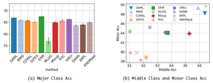
Figure 1: (a) Average accuracy of target data in major classes in open domain Office-Home. The major class indicates the class appeared in three source domains. (b) Average accuracy of target data in middle and minor classes in open domain Office-Home. The middle and minor classes indicate the classes that appeared in two and one source domains, respectively.

4.2 Methods

We evaluated a baseline method (ERM), an OSR method (ARPL), nine DG methods including CORAL and MMD, an ODG method (DAML), as listed below, in addition to the extended methods of CORAL and MMD proposed in Section 3.2.

• Baseline method (ERM [27]): A method without any handling for domain shift or OSR, which only minimizes the cross entropy loss for source domain datasets.

• OSR method (ARPL [1]): A state-of-the-art method for OSR, but it does not deal with domain shift.

• DG methods (CORAL, MMD, ANDMASK [18], DANN [5], MLDG [13], Mixup [32], RSC [11], V-REx [12], and DIFEX [16]): These methods were used for DG scenario.

• ODG method (DAML [24]): A method proposed for ODG.

The DG methods were selected from those evaluated in [8, 30], and the same implementation was used in [8, 30]. Among the DG methods used in our experiment, MLDG and RSC have been evaluated in [24] for ODG, while the other seven DG methods have not yet been evaluated in ODG.

The feature extractors used for each method were the pre-trained ResNet-18 [9] on ImageNet [3]. We evaluated the model with the best performance on the validation data. The data augmentation is the same as in the literature [8]. Detailed experimental settings can be found in the supplementary material.

Two evaluation metrics were used: Accuracy (Acc) and H-score [4], where Acc evaluates the accuracy of a known class classification and H-score equally evaluates known class classification and unknown class detection. The calculation method of H-score is the same as in [24].

Table 5: Results of PACS dataset under the open-domain setting. Bold values represent the best value, underlined values represent the second-best value, and values in parentheses represent the standard deviation.

	Art		Cartoon		Photo		Sketch		Avg.
Method	Acc	H-score	Acc	H-score	Acc	H-score	Acc	H-score	Acc	H-score
ERM	51.57	43.82	48.53	41.82	57.13	60.00	41.54	36.61	49.69 (1.17)	45.56 (1.27)
ARPL	53.47	45.19	52.86	42.33	56.70	56.51	46.55	37.83	52.39 (1.81)	45.47 (1.27)
ANDMask	50.51	42.64	57.31	48.45	57.35	18.90	47.29	40.29	53.11 (0.85)	37.57 (2.23)
DANN	51.67	42.64	57.09	47.24	51.56	43.58	45.64	38.16	51.49 (2.68)	42.90 (1.89)
DIFEX	46.24	40.38	50.66	44.13	49.11	10.84	43.10	40.41	47.27 (0.90)	33.94 (2.26)
MLDG	48.53	41.11	44.45	42.30	61.04	64.77	40.97	36.40	48.75 (1.88)	46.14 (0.53)
Mixup	52.67	42.59	53.18	44.93	58.13	58.63	43.86	37.38	51.96 (1.29)	45.88 (0.56)
RSC	50.40	36.54	52.07	46.72	53.04	48.48	44.40	37.57	49.98 (0.99)	42.33 (0.66)
VREx	51.86	43.90	50.04	42.38	57.05	59.01	41.47	35.72	50.10 (1.34)	45.25 (1.46)
CORAL	53.72	47.24	55.89	46.21	71.13	70.53	51.95	47.20	58.17 (1.96)	52.79 (1.36)
MMD	53.38	44.26	55.30	45.96	68.04	69.79	54.24	47.20	57.74 (4.23)	51.80 (1.64)
DAML	59.32	51.62	66.70	53.25	81.01	63.68	62.97	53.30	67.50 (1.80)	55.46 (4.31)

Table 6: Results of Office-Home dataset under the open-domain setting. Bold values represent the best value, underlined values represent the second-best value, and values in parentheses represent the standard deviation.

	Art		Clipart		Product		Real World		Avg.
Method	Acc	H-score	Acc	H-score	Acc	H-score	Acc	H-score	Acc	H-score
ERM	44.01	43.84	48.13	44.72	56.32	54.20	64.44	57.75	53.22 (0.74)	50.13 (0.12)
ARPL	40.84	42.13	45.04	42.73	53.48	52.31	59.59	54.59	49.73 (0.63)	47.94 (0.28)
ANDMask	40.36	41.10	42.98	41.62	54.32	53.38	61.82	55.01	49.87 (0.72)	47.77 (0.21)
DANN	47.04	45.26	42.86	41.44	56.43	51.74	65.76	58.47	53.02 (0.25)	49.23 (0.32)
DIFEX	40.67	40.93	44.20	43.22	52.86	50.84	60.75	54.67	49.62 (0.21)	47.41 (0.21)
MLDG	44.06	44.12	44.33	46.23	54.92	53.29	64.02	58.49	51.83 (0.58)	50.53 (1.52)
Mixup	46.09	46.11	46.60	44.08	57.14	54.97	65.34	58.99	53.79 (0.25)	51.03 (0.50)
RSC	40.07	40.11	44.79	42.38	52.91	53.62	59.33	55.31	49.27 (0.10)	47.85 (0.41)
VREx	44.36	44.59	46.90	43.68	56.86	54.43	64.60	57.84	53.18 (0.80)	50.13 (0.15)
CORAL	50.33	47.28	49.97	47.67	60.49	56.15	68.47	61.94	57.31 (0.70)	53.26 (0.34)
MMD	49.91	47.13	49.51	46.82	59.62	55.57	68.60	61.63	56.91 (0.13)	52.79 (0.58)
DAML	47.64	46.27	51.56	49.41	59.98	56.97	67.40	62.22	56.65 (0.89)	53.72 (0.43)

Table 7: Results of Multi-Datasets. Bold values represent the best value, underlined values represent the second-best value, and values in parentheses represent the standard deviation.

	Clipart		Sketch		Painting		Real		Avg.
Method	Acc	H-score	Acc	H-score	Acc	H-score	Acc	H-score	Acc	H-score
ERM	35.09	38.47	28.89	33.14	48.75	51.65	67.68	64.77	45.10 (1.13)	47.01 (0.83)
ARPL	32.02	34.62	27.24	31.14	46.30	49.12	64.21	61.72	42.44 (0.65)	44.15 (0.47)
ANDMask	35.33	37.73	29.54	31.20	39.72	42.04	60.21	56.13	41.20 (1.15)	41.77 (1.07)
DANN	34.43	36.79	27.97	29.68	43.02	44.95	60.72	56.64	41.54 (1.48)	42.01 (1.16)
DIFEX	30.27	34.30	27.45	30.68	38.49	42.70	60.13	59.64	39.08 (2.19)	41.83 (1.73)
MLDG	28.43	32.78	33.45	37.75	41.88	44.41	55.01	57.69	39.69 (2.10)	43.16 (2.47)
Mixup	36.92	37.55	26.85	30.18	44.75	46.61	66.15	62.71	43.67 (2.01)	44.26 (2.61)
RSC	31.12	33.91	21.79	25.48	39.42	42.52	62.29	59.54	38.65 (1.22)	40.36 (1.01)
VREx	36.11	38.44	28.83	32.07	48.83	50.95	67.58	64.29	45.34 (0.61)	46.44 (0.77)
CORAL	40.80	42.26	34.02	37.76	45.53	48.91	65.98	64.45	46.58 (1.20)	48.35 (0.89)
MMD	39.17	41.23	34.25	37.72	46.37	49.48	66.22	64.54	46.50 (0.77)	48.24 (0.82)
DAML	42.69	44.38	34.43	37.38	45.53	47.85	62.77	63.00	46.35 (2.38)	48.15 (2.02)

Table 8: Comparison of the average Acc and H-score values of CORAL, MMD, DAML, and their derivatives across all test domains for each dataset, averaging the performance for the four test domains for each dataset per trial, and showing the three-trial average of the average values. Bold numbers represent the best values, underlined numbers represent the second-best values, and values in parentheses represent the standard deviation.

	PACS		Office-Home		Multi-Datasets
Method	Acc	H-score	Acc	H-score	Acc	H-score
CORAL	58.17 (1.96)	52.79 (1.36)	57.31 (0.70)	53.26 (0.34)	46.58 (1.20)	48.35 (0.89)
E-CORAL	59.50 (1.24)	43.23 (3.97)	58.15 (0.06)	53.46 (0.19)	48.38 (0.54)	49.13 (0.62)
EDir-CORAL	68.27 (1.87)	53.86 (1.81)	57.44 (0.18)	53.96 (0.23)	46.55 (0.82)	49.43 (0.70)
EDst-CORAL	66.25 (1.86)	53.10 (3.17)	57.81 (0.98)	53.86 (0.63)	46.60 (0.91)	48.34 (1.54)
MMD	57.74 (4.23)	51.80 (1.64)	56.91 (0.13)	52.79 (0.58)	46.50 (0.77)	48.24 (0.82)
E-MMD	58.60 (0.57)	49.08 (0.85)	58.61 (0.80)	53.55 (0.27)	47.47 (1.60)	47.60 (1.50)
EDir-MMD	67.52 (3.08)	55.53 (2.56)	57.10 (0.18)	53.61 (0.45)	45.78 (2.29)	47.67 (1.80)
EDst-MMD	65.68 (3.10)	53.32 (3.03)	56.46 (0.37)	53.21 (0.48)	46.15 (0.48)	47.92 (0.76)
DAML	67.50 (1.80)	55.46 (4.31)	56.65 (0.89)	53.72 (0.43)	46.35 (2.38)	48.15 (2.02)
DAML w/o Dir	66.49 (0.93)	55.99 (0.72)	57.34 (0.73)	53.62 (0.49)	46.51 (1.06)	47.94 (0.83)
DAML w/o Dst	67.28 (2.60)	55.57 (1.38)	56.45 (0.31)	53.34 (0.34)	45.49 (2.43)	48.23 (2.51)
DAML w/o Dir-Dst	64.91 (1.62)	53.73 (1.05)	57.80 (0.35)	53.59 (0.50)	46.51 (0.94)	48.42 (1.07)

4.3 Experimental Results and Discussion

4.3.1 Evaluation of Conventional DG Methods

Tables 5, 6 and 7 show the mean Acc and H-score over three trials for each target domain of PACS, Office-Home, and Multi-Datasets, respectively. From Table 5, we observe that DAML exhibits superior performance than other methods for most target domains on open domain PACS datasets. We also observe that CORAL and MMD show the second-best performance. Tables 6 and 7, the results of the open domain Office-Home and Multi-Datasets, show that CORAL and MMD achieved comparable performance with DAML in both Acc and H-score. These results imply the simple DG methods, CORAL and MMD, have the potential for ODG even compared to complicated DAML.

Figure 1 shows the accuracy of the major, middle, and minor classes in open domain Office-Home. The major, middle, and minor classes indicate the classes that appeared in three, two, and one source domains, respectively. In the major class, DAML, MMD, and CORAL are not significantly better than the other methods and are inferior to the baseline method ERM. On the other hand, DAML, MMD, and CORAL outperform the other methods in the middle and minor classes, suggesting that these methods perform well in ODG because they can predict classes with fewer domains better than the other methods.

4.3.2 Evaluation of Extended CORAL and MMD

Table 8 compares the average Acc and H-score of CORAL, MMD, DAML, and their variations for the target domains. In addition to the extended versions of CORAL and MMD, we evaluate the variations of DAML: DAML without Dir-mixup for meta-training and meta-objective losses (DAML w/o Dir), DAML without knowledge distillation (DAML w/o Dst), and DAML without both Dir-mixup and knowledge distillation (DAML w/o Dir-Dst).

For the open domain PACS, EDir-CORAL and EDir-MMD have succeeded in improving the performance and show comparable performance to DAML. This result indicates that the Dir-mixup data augmentation is effective for both CORAL and MMD in the open-domain PACS. On the other hand, DAML and DAML w/o Dir exhibit similar performance, implying that knowledge distillation and meta-learning other than Dir-mixup data augmentation contribute to the performance improvement of DAML. In the open domain Office-Home and Multi-Datasets, the Dir-mixup data augmentation shows little improvement for CORAL and MMD. This might be because data augmentation is not effective for Office-Home and Multi-Datasets.

The experimental result shows that the simple extensions of CORAL and MMD can enhance the performance and achieve comparable or better performances to DAML.

Table 9: Comparison of average Acc for each dataset on the source domains over three trials. For each trial, the average ACC for three source domains over four experimental settings is calculated. Bold numbers represent the best value, underlined numbers represent the second-best value, and values in parentheses represent the standard deviation.

Method	PACS	Office-Home	Multi-Datasets
ERM	97.33 (0.19)	83.86 (0.30)	93.30 (0.52)
CORAL	90.35 (1.65)	81.56 (0.51)	89.86 (0.52)
E-CORAL	97.48 (0.12)	84.77 (0.26)	94.41 (0.07)
EDir-CORAL	92.97 (0.22)	83.79 (0.41)	89.93 (0.51)
EDst-CORAL	92.64 (0.57)	83.64 (0.46)	90.06 (0.52)
MMD	89.89 (1.74)	81.30 (0.55)	89.50 (0.35)
E-MMD	97.59 (0.22)	85.47 (0.26)	94.30 (0.34)
EDir-MMD	92.77 (0.72)	83.65 (0.41)	89.93 (0.91)
EDst-MMD	92.65 (0.36)	83.40 (0.46)	89.77 (0.31)
DAML	94.05 (0.63)	83.84 (0.04)	89.11 (0.23)
DAML w/o Dir	93.40 (0.05)	83.71 (0.16)	90.03 (0.87)
DAML w/o Dst	94.23 (0.63)	83.55 (0.12)	89.78 (0.43)
DAML w/o Dir-Dst	93.16 (0.28)	83.42 (0.39)	90.60 (0.62)

Table 10: Comparison of learning times (in seconds) per epoch on one GPU. average learning times were measured for four different target domains on each dataset per trial, and the average of the average learning times over three trials is shown. Bold numbers represent the best value, underlined numbers represent the second-best value, and values in parentheses represent the standard deviation.

Method	PACS	Office-Home	Multi-Datasets
ERM	6.368 (0.007)	15.92 (0.04)	6.424 (0.014)
CORAL	10.29 (0.07)	16.76 (0.05)	10.14 (1.05)
E-CORAL	13.88 (0.02)	17.59 (0.17)	13.95 (0.02)
EDir-CORAL	17.33 (0.02)	18.46 (0.26)	17.40 (0.05)
EDst-CORAL	17.23 (0.01)	18.61 (0.35)	17.30 (0.10)
MMD	10.21 (0.12)	16.60 (0.14)	10.36 (0.39)
E-MMD	14.39 (0.01)	17.63 (0.19)	14.45 (0.03)
EDir-MMD	19.22 (0.07)	19.34 (0.11)	19.24 (0.05)
EDst-MMD	19.05 (0.02)	19.43 (0.21)	19.01 (0.04)
DAML	32.86 (0.08)	32.96 (0.05)	33.08 (0.13)
DAML w/o Dir	24.85 (0.12)	24.81 (0.11)	24.79 (0.18)
DAML w/o Dst	32.85 (0.06)	32.92 (0.07)	32.81 (0.09)
DAML w/o Dir-Dst	24.56 (0.15)	24.64 (0.10)	24.54 (0.25)

4.3.3 Evaluation on Source Domains

Table 9 exports the test performance of each method on source domains, i.e., the case where no domain shift occurs and only known classes appear. We believe evaluating the methods on source domains is important because we may not know whether the domain shift will occur in a practical use case. The extended versions of CORAL and MMD show good performances for all datasets. In particular, E-CORAL and E-MMD exhibit the best performance and outperform ERM. Therefore, simple ensemble learning will be effective for no or small domain shifts.

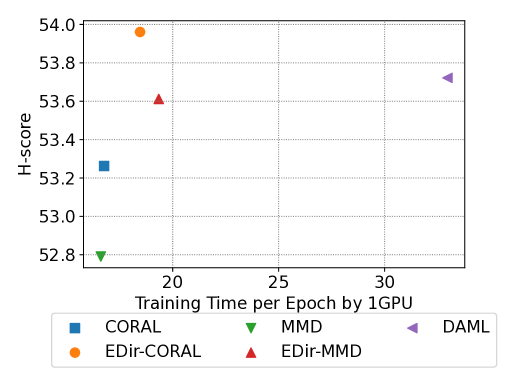
Figure 2: Scatterplot of H-score and training time per epoch (in seconds) for each method on the open domain Office-Home.

4.3.4 Computational Cost

Table 10 compares the average training time per epoch of the variations of CORAL, MMD, and DAML. The model training uses one NVIDIA A100 (80GB) GPU. For all datasets, the training times of the variations of CORAL and MMD were less than that of DAML. This is because our CORAL and MMD variations update the model parameters by minimizing one loss function, whereas DAML alternatively minimizes two types of loss functions. Note that, unlike DAML, E-CORAL and E-MMD can train each model in parallel, which can further reduce the training time by using more GPUs to the same level as that of CORAL and MMD.

Figure 2 summarizes the relationship between the H-score for the target domain and training time on the open domain Office-Home. We observe that EDir-CORAL and EDir-MMD achieve the comparable H-score as DAML at a lower training time cost than DAML. We have shown that the simple DG methods, CORAL and MMD, can achieve state-of-the-art performance with less computational cost by using simple extensions.

5 Conclusion

In this paper, we have comprehensively evaluated DG methods on open-set recognition during domain shift. We found that the classic DG methods, CORAL and MMD, are comparable to DAML proposed for ODG in two datasets out of three. We have also proposed and evaluated the extended versions of CORAL and MMD that are injected with the techniques used in DAML. We have shown that EDir-CORAL and EDir-MMD can reach comparable performances with DAML on all datasets with lower training costs. We hope that this work will be exploited as the baseline for further development of the ODG methods. A possible future work is to evaluate the DG methods, including our extended versions, in the ODG situations of other tasks, such as speech and natural language processing.

Appendix A Definitions of Domain Generalization and Open Domain Generalization

This section describes the definitions of domain generalization (DG) and open domain generalization (ODG).

A.1 Domain Generalization (DG)

Let us consider classification problems and denote the input and class spaces as $\mathcal{X}$ and $C$, respectively. We have $M$ multiple labeled source datasets (domains), $\mathcal{D}_{1},\dots,\mathcal{D}_{M}$, where $\mathcal{D}_{s}=\left\{\left(\mathbf{x}_{s}^{i},\mathbf{y}_{s}^{i}\right)\right\}_{i=1}^{N_{s}}$, $(\mathbf{x}_{s}^{i},\mathbf{y}_{s}^{i})\in\mathcal{X}\times C$, and $N_{s}$ indicates the number of data in the $s$-th dataset. The goal of DG is to obtain a model that correctly predicts the known classes of unseen input data $\{\mathbf{x}_{t}\}_{i=1}^{N_{t}}$ in a target domain $\mathcal{D}_{t}$ using multiple source domains. In DG, the data distributions of the source and target domains $\mathcal{D}_{1},\dots,\mathcal{D}_{M},\mathcal{D}_{t}$ are different, but the class spaces are identical, i.e., $\mathbf{y}_{s}^{i},\mathbf{y}_{t}^{i}\in C$.

A.2 Open Domain Generalization (ODG)

In ODG [24], the class spaces of the source and target domains are different, which is the difference between DG and ODG and the difficulty of ODG compared to DG. First, the class spaces of the source domains can be different, as shown in Figure 3. Therefore, the class spaces of the $p$- and $q$-th source domains may differ, $C_{p}\neq C_{q}$. Second, the target domain has novel classes that do not belong to any source domain. Let $C=\bigcup_{k=1}^{M}C_{k}$ be the union of all source class spaces; then we denote the target class space $C_{t}=C\cup C_{u}$, where $C_{u}$ is the novel class space that first appears in the test phase. The goal of ODG is to obtain a model that correctly classifies unseen target samples $\{\mathbf{x}_{t}\}_{i=1}^{N_{t}}$ into $\left|C\right|+1$ classes, that is, classifying samples belonging to known classes $C$ into the correct class and treating samples belonging to novel classes $C_{u}$ as one unknown class. We note that the data distributions of the source and target domains $\mathcal{D}_{1},\dots,\mathcal{D}_{M},\mathcal{D}_{t}$ are different as in DG.

Appendix B Detailed Experimental Setting

We list the common settings and hyperparameters of each algorithm in Tables 11 and 12, respectively. We determined the hyperparameter values based on literature [8, 30].

Table 11: Common experimental settings.

Parameter	Value
Trials	3
Feature extractor	ResNet-18 [9]
Optimizer	Momentum SGD
Coefficient of inertia term	0.9
Batch size	32
Num. of Training Epochs	100
Early stopping epochs	10
Learning rate	0.001

Table 12: Hyperparameters of each algorithm, which is set based on literature [8, 30].

Algorithm	Parameter	Value
ARPL	lambda temperature margin	0.1 1.0 1.0
ANDMask	tau	1.0
DANN	alpha	1.0
DIFEX	beta dist type	1.0 2-norm
MLDG	beta	1.0
Mixup	alpha	0.2
RSC	feature drop factor batch drop factor	0.33 0.33
VREx	warmup iterations lamda	500 1.0
CORAL	gamma	1.0
MMD	gamma	1.0
DAML	softmax temperature trade trade2 trade3 trade4 max alpha min alpha meta step size	2.0 3.0 1.0 1.0 3.0 0.6 0.2 0.01

Figure 3 shows the illustration of the class space for each dataset. We note that open domain PACS and Multi-Datasets do not have a major class that appeared in all three source domains.

Our experimental codes for all experiments will be made publicly available upon publication.

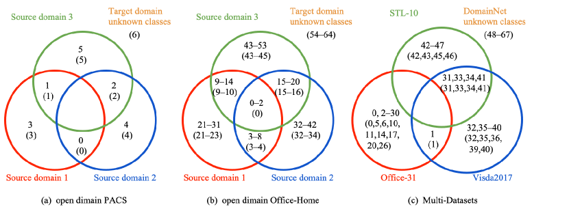
Figure 3: Illustration of the class space for each dataset. Indices without brackets show the distribution of classes among source domains, while indices in brackets indicate the classes of the target domain.

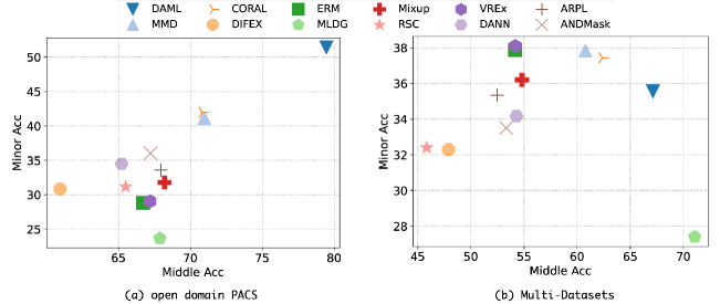
Figure 4: Scatterplot of middle and minor class Acc for (a) open domain PACS and (b) Multi-Datasets.

Appendix C Detailed Experimental Results

In this section, we describe the accuracy of the middle and minor classes in open domain PACS and Multi-Datasets. Also, we show an evaluation of CORAL, MMD, DAML, and their variations in the target domain. Finally, we report the computational cost of CORAL, MMD, DAML, and their variations.

C.1 Accuracy of Middle and Minor Classes in Open Domain PACS and Multi-Datasets

Figure 4 shows the accuracy of the middle and minor classes in open domain PACS and Multi-Datasets by existing methods. The middle and minor classes indicate the classes that appeared in two and one source domains, respectively. In the open domain PACS, DAML, MMD, and CORAL outperform the other methods in the middle and minor classes. In Multi-Datasets, DAML, MMD, and CORAL also outperform the other methods except for MLDG in the middle class but are not much superior to other methods in the minor class. Note that open domain PACS and Multi-Datasets do not have a major class.

C.2 Evaluation of CORAL, MMD, DAML, and Their variations on Target Domain

Tables 13, 14, and 15 show the mean Acc and H-score over three trials by CORAL, MMD, DAML, and their variations for each target domain of PACS, Office-Home, and Multi-Datasets, respectively. From Table 13, we observe that, in the open domain PACS, EDir-CORAL and EDir-MMD outperform CORAL and MMD for any target domain, showing the effectiveness of Dir-mixup data augmentation. On the other hand, Tables 14 and 14 show that EDir-CORAL and EDir-MMD have slightly better or similar performance for most target domains compared to CORAL and MMD.

Table 13: Results of CORAL, MMD, DAML, and their variations in the PACS dataset under the open-domain setting. Bold values represent the best value, underlined values represent the second-best value, and values in parentheses represent the standard deviation.

	Art		Cartoon		Photo		Sketch		Avg
Method	Acc	H-score	Acc	H-score	Acc	H-score	Acc	H-score	Acc	H-score
CORAL	53.72	47.24	55.89	46.21	71.13	70.53	51.95	47.20	58.17(1.96)	52.79(1.36)
E-CORAL	59.16	47.72	59.62	49.59	63.41	33.29	55.83	42.34	59.50(1.24)	43.23(3.97)
EDir-CORAL	58.66	49.67	67.18	53.31	83.25	60.30	63.98	52.15	68.27(1.87)	53.86(1.81)
EDst-CORAL	61.78	48.74	64.81	48.43	80.02	64.98	58.38	50.24	66.25(1.86)	53.10(3.17)
MMD	53.38	44.26	55.30	45.96	68.04	69.79	54.24	47.20	57.74(4.23)	51.80(1.64)
E-MMD	57.55	48.23	57.33	46.33	64.43	59.48	55.11	42.26	58.60(0.57)	49.08(0.85)
EDir-MMD	59.56	49.79	66.40	51.35	79.59	67.49	64.53	53.51	67.52(3.08)	55.53(2.56)
EDst-MMD	59.45	48.67	62.97	46.71	78.73	64.86	61.59	53.05	65.68(3.10)	53.32(3.03)
DAML	59.32	51.62	66.70	53.25	81.01	63.68	62.97	53.30	67.50(1.80)	55.46(4.31)
DAML w/o Dir	61.70	51.44	64.65	52.44	83.38	71.61	56.22	48.49	66.49(0.93)	55.99(0.72)
DAML w/o Dst	60.43	51.08	67.20	53.47	80.42	67.73	61.08	50.00	67.28(2.60)	55.57(1.38)
DAML w/o Dir-Dst	61.01	52.07	63.78	48.24	83.14	69.89	51.71	44.74	64.91(1.62)	53.73(1.05)

Table 14: Results of CORAL, MMD, DAML, and their variations in the Office-Home dataset under the open-domain setting. Bold values represent the best value, underlined values represent the second-best value, and values in parentheses represent the standard deviation.

	Art		Clipart		Product		Real World		Avg
Method	Acc	H-score	Acc	H-score	Acc	H-score	Acc	H-score	Acc	H-score
CORAL	50.33	47.28	49.97	47.67	60.49	56.15	68.47	61.94	57.31(0.70)	53.26(0.34)
E-CORAL	50.56	46.92	51.77	47.37	60.78	57.30	69.50	62.27	58.15(0.06)	53.46(0.19)
EDir-CORAL	48.24	47.40	53.03	48.70	59.62	56.93	68.89	62.80	57.44(0.18)	53.96(0.23)
EDst-CORAL	47.76	46.33	54.23	51.29	59.76	55.98	68.41	61.85	57.81(0.98)	53.86(0.63)
MMD	49.91	47.13	49.51	46.82	59.62	55.57	68.60	61.63	56.91(0.13)	52.79(0.58)
E-MMD	51.28	47.09	51.22	47.31	61.42	57.19	70.51	62.64	58.61(0.80)	53.55(0.27)
EDir-MMD	46.33	45.78	52.63	48.76	61.34	57.55	68.12	62.34	57.10(0.18)	53.61(0.45)
EDst-MMD	47.10	45.76	51.87	49.03	59.96	56.01	66.92	62.04	56.46(0.37)	53.21(0.48)
DAML	47.64	46.27	51.56	49.41	59.98	56.97	67.40	62.22	56.65(0.89)	53.72(0.43)
DAML w/o Dir	47.76	46.18	52.39	49.08	60.13	56.37	69.09	62.84	57.34(0.73)	53.62(0.49)
DAML w/o Dst	45.97	45.67	52.35	48.00	60.07	58.37	67.41	61.31	56.45(0.31)	53.34(0.34)
DAML w/o Dir-Dst	49.85	47.24	51.62	48.43	60.38	56.30	69.38	62.40	57.80(0.35)	53.59(0.50)

Table 15: Results of CORAL, MMD, DAML, and their variations in Multi-Datasets. Bold values represent the best value, underlined values represent the second-best value, and values in parentheses represent the standard deviation.

	Clipart		Sketch		Painting		Real		Avg
Method	Acc	H-score	Acc	H-score	Acc	H-score	Acc	H-score	Acc	H-score
CORAL	40.80	42.26	34.02	37.76	45.53	48.91	65.98	64.45	46.58(1.20)	48.35(0.89)
E-CORAL	40.97	42.41	33.67	35.94	49.65	52.15	69.22	66.04	48.38(0.54)	49.13(0.62)
EDir-CORAL	41.42	44.46	37.72	41.03	44.69	48.99	62.37	63.24	46.55(0.82)	49.43(0.70)
EDst-CORAL	41.99	44.59	35.29	37.25	44.19	47.38	64.95	64.15	46.60(0.91)	48.34(1.54)
MMD	39.17	41.23	34.25	37.72	46.37	49.48	66.22	64.54	46.50(0.77)	48.24(0.82)
E-MMD	39.70	40.45	31.95	33.90	48.53	50.17	69.70	65.89	47.47(1.60)	47.60(1.50)
EDir-MMD	40.27	42.29	35.56	37.97	44.00	47.35	63.31	63.08	45.78(2.29)	47.67(1.80)
EDst-MMD	40.80	43.68	35.67	37.32	43.43	46.70	64.71	63.99	46.15(0.48)	47.92(0.76)
DAML	42.69	44.38	34.43	37.38	45.53	47.85	62.77	63.00	46.35(2.38)	48.15(2.02)
DAML w/o Dir	40.89	42.47	35.95	38.26	44.60	48.04	64.60	62.99	46.51(1.06)	47.94(0.83)
DAML w/o Dst	41.09	44.22	34.18	37.47	44.66	48.74	62.03	62.52	45.49(2.43)	48.23(2.51)
DAML w/o Dir-Dst	40.23	42.92	35.79	38.64	45.05	48.32	64.97	63.80	46.51(0.94)	48.42(1.07)

C.3 Computational Cost

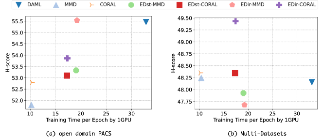
Figure 5: Scatterplot of H-score and training time for open domain PACS and Multi-Datasets.

Figure 5 compares the average training time per epoch of the variations of CORAL and MMD, and DAML. We used an NVIDIA A100 (80GB) GPU for model training. The tendency of the training times is the same as in the open domain Office-Home. For both open domain PACS and Multi-Datasets, the training times of the variations of CORAL and MMD were less than that of DAML.

References

- [1] Guangyao Chen, Peixi Peng, Xiangqian Wang, and Yonghong Tian. Adversarial reciprocal points learning for open set recognition. IEEE Transactions on Pattern Analysis and Machine Intelligence, 2022.
- [2] Adam Coates, Andrew Ng, and Honglak Lee. An analysis of single-layer networks in unsupervised feature learning. In Proceedings of the Fourteenth International Conference on Artificial Intelligence and Statistics. PMLR, 2011.
- [3] Jia Deng, Wei Dong, Richard Socher, Li-Jia Li, Kai Li, and Li Fei-Fei. Imagenet: A large-scale hierarchical image database. In 2009 IEEE Conference on Computer Vision and Pattern Recognition, 2009.
- [4] Bo Fu, Zhangjie Cao, Mingsheng Long, and Jianmin Wang. Learning to Detect Open Classes for Universal Domain Adaptation. In European Conference on Computer Vision (ECCV). Springer, 2020.
- [5] Yaroslav Ganin, Evgeniya Ustinova, Hana Ajakan, Pascal Germain, Hugo Larochelle, François Laviolette, Mario Marchand, and Victor Lempitsky. Domain-adversarial training of neural networks. Journal of Machine Learning Research, 2016.
- [6] Chuanxing Geng, Sheng-jun Huang, and Songcan Chen. Recent advances in open set recognition: A survey. IEEE Transactions on Pattern Analysis and Machine Intelligence, 2020.
- [7] Arthur Gretton, Karsten M. Borgwardt, Malte J. Rasch, Bernhard Schölkopf, and Alexander Smola. A kernel two-sample test. Journal of Machine Learning Research, 2012.
- [8] Ishaan Gulrajani and David Lopez-Paz. In search of lost domain generalization. In International Conference on Learning Representations, 2020.
- [9] Kaiming He, Xiangyu Zhang, Shaoqing Ren, and Jian Sun. Deep Residual Learning for Image Recognition. In International Conference on Computer Vision and Pattern Recognition, pages 770–778, 2016.
- [10] Dan Hendrycks and Thomas Dietterich. Benchmarking neural network robustness to common corruptions and perturbations. In International Conference on Learning Representations, 2018.
- [11] Zeyi Huang, Haohan Wang, Eric P Xing, and Dong Huang. Self-challenging improves cross-domain generalization. In European Conference on Computer Vision, pages 124–140. Springer, 2020.
- [12] David Krueger, Ethan Caballero, Joern-Henrik Jacobsen, Amy Zhang, Jonathan Binas, Dinghuai Zhang, Remi Le Priol, and Aaron Courville. Out-of-distribution generalization via risk extrapolation. In Proceedings of the International Conference on Machine Learning. PMLR, 2021.
- [13] Da Li, Yongxin Yang, Yi-Zhe Song, and Timothy Hospedales. Learning to generalize: Meta-learning for domain generalization. In Proceedings of the AAAI conference on artificial intelligence, 2018.
- [14] Da Li, Yongxin Yang, Yi-Zhe Song, and Timothy M. Hospedales. Deeper, broader and artier domain generalization. In Proceedings of the IEEE International Conference on Computer Vision (ICCV), 2017.
- [15] Haoliang Li, Sinno Jialin Pan, Shiqi Wang, and Alex C Kot. Domain generalization with adversarial feature learning. In Proceedings of the IEEE Conference on Computer Vision and Pattern Recognition, 2018.
- [16] Wang Lu, Jindong Wang, Haoliang Li, Yiqiang Chen, and Xing Xie. Domain-invariant feature exploration for domain generalization. Transactions on Machine Learning Research, 2022.
- [17] Atefeh Mahdavi and Marco Carvalho. A survey on open set recognition. In 2021 IEEE Fourth International Conference on Artificial Intelligence and Knowledge Engineering (AIKE). IEEE, 2021.
- [18] Giambattista Parascandolo, Alexander Neitz, ANTONIO ORVIETO, Luigi Gresele, and Bernhard Schölkopf. Learning explanations that are hard to vary. In International Conference on Learning Representations, 2021.
- [19] Xingchao Peng, Qinxun Bai, Xide Xia, Zijun Huang, Kate Saenko, and Bo Wang. Moment matching for multi-source domain adaptation. In 2019 IEEE/CVF International Conference on Computer Vision (ICCV), 2019.
- [20] Xingchao Peng, Ben Usman, Neela Kaushik, Dequan Wang, Judy Hoffman, and Kate Saenko. Visda: A synthetic-to-real benchmark for visual domain adaptation. In 2018 IEEE/CVF Conference on Computer Vision and Pattern Recognition Workshops (CVPRW), 2018.
- [21] Joaquin Quinonero-Candela, Masashi Sugiyama, Anton Schwaighofer, and Neil D Lawrence. Dataset shift in machine learning. Mit Press, 2008.
- [22] Kate Saenko, Brian Kulis, Mario Fritz, and Trevor Darrell. Adapting visual category models to new domains. In European Conference on Computer Vision, Lecture Notes in Computer Science. Springer, 2010.
- [23] Kuniaki Saito, Shohei Yamamoto, Yoshitaka Ushiku, and Tatsuya Harada. Open set domain adaptation by backpropagation. In Proceedings of the European Conference on Computer Vision (ECCV), 2018.
- [24] Yang Shu, Zhangjie Cao, Chenyu Wang, Jianmin Wang, and Mingsheng Long. Open domain generalization with domain-augmented meta-learning. In Proceedings of the IEEE/CVF Conference on Computer Vision and Pattern Recognition, 2021.
- [25] Baochen Sun and Kate Saenko. Deep coral: Correlation alignment for deep domain adaptation. In European Conference on Computer Vision. Springer, 2016.
- [26] Vivienne Sze, Yu-Hsin Chen, Tien-Ju Yang, and Joel S Emer. Efficient processing of deep neural networks: A tutorial and survey. Proceedings of the IEEE, 2017.
- [27] Vladimir Vapnik, Vlamimir Vapnik, et al. Statistical learning theory, 1998.
- [28] Sagar Vaze, Kai Han, Andrea Vedaldi, and Andrew Zisserman. Open-set recognition: A good closed-set classifier is all you need. In International Conference on Learning Representations, 2022.
- [29] Hemanth Venkateswara, Jose Eusebio, Shayok Chakraborty, and Sethuraman Panchanathan. Deep hashing network for unsupervised domain adaptation. In Proceedings of the IEEE Conference on Computer Vision and Pattern Recognition (CVPR), 2017.
- [30] Jindong Wang, Cuiling Lan, Chang Liu, Yidong Ouyang, Tao Qin, Wang Lu, Yiqiang Chen, Wenjun Zeng, and Philip Yu. Generalizing to unseen domains: A survey on domain generalization. IEEE Transactions on Knowledge and Data Engineering, 2022.
- [31] Shiqi Yang, Yaxing Wang, Kai Wang, Shangling Jui, and Joost van de Weijer. One ring to bring them all: Towards open-set recognition under domain shift. arXiv preprint arXiv:2206.03600, 2022.
- [32] Hongyi Zhang, Moustapha Cisse, Yann N Dauphin, and David Lopez-Paz. mixup: Beyond empirical risk minimization. In International Conference on Learning Representations, 2018.
- [33] Kaiyang Zhou, Ziwei Liu, Yu Qiao, Tao Xiang, and Chen Change Loy. Domain generalization: A survey. IEEE Transactions on Pattern Analysis and Machine Intelligence, 2021.
- [34] Ronghang Zhu and Sheng Li. Crossmatch: Cross-classifier consistency regularization for open-set single domain generalization. In International Conference on Learning Representations, 2022.