PYATB: An Efficient Python Package for Electronic Structure Calculations Using Ab Initio Tight-Binding Model

Abstract

We present PYATB, a Python package designed for computing band structures and related properties of materials using the ab initio tight-binding Hamiltonian. The Hamiltonian is directly obtained after conducting self-consistent calculations with first-principles packages using numerical atomic orbital (NAO) bases, such as ABACUS. The package comprises three modules: Bands, Geometric, and Optical. In the Bands module, one can calculate essential properties of band structures, including the partial density of states (PDOS), fat bands, Fermi surfaces, and Weyl/Dirac points. The band unfolding method is utilized to obtain the energy band spectra of a supercell by projecting the electronic structure of the supercell onto the Brillouin zone of the primitive cell. With the Geometric module, one can compute the Berry phase and Berry curvature-related quantities, such as electric polarization, Wilson loops, Chern numbers, and anomalous Hall conductivities. The Optical module offers a range of optical property calculations, including optical conductivity and nonlinear optical responses, such as shift current and Berry curvature dipole.

PROGRAM SUMMARY

Program Title: PYATB
CPC Library link to program files: (to be added by Technical Editor)
Developer’s repository link: https://github.com/pyatb/pyatb
Code Ocean capsule: (to be added by Technical Editor)
Licensing provisions: GPLv3
Programming language: C++, Python
Nature of problem: This program is to study the electronic structure, electronic polarization, band topological properties, topological classification, linear and nonlinear optical response of solid crystal systems.
Solution method: Based on the tight binding method to solve the band structure, the Wilson loop is used to classify the topological phases, and the optical response is calculated by Berry curvature and Berry connection.

1 Introduction

Electronic band structures are critical in determining the physical properties of solids, including their optical, transport, and topological properties. For instance, in materials with nontrivial topological properties, such as topological insulators [1, 2, 3], topological crystalline insulators [4], Dirac [5, 6] and Weyl semimetals [7, 8, 9], and nodal-line semimetals [10, 11, 12], calculations of the Berry curvature [13], Chern number [14], and Wannier charge centers [15] are crucial for understanding these topological states. Moreover, recent studies have revealed that the Berry connection and Berry curvature also play essential roles in various nonlinear optical effects [16, 17]. Kohn-Sham density functional theory [18, 19] is a vital tool for calculating band structures and their associated properties. However, these calculations typically require a large number of $\mathbf{k}$ points, making them computationally demanding. The tight-binding model offers an efficient approach to investigating electronic structures in materials. In plane wave-based codes, the Maximally Localized Wannier Functions (MLWF) method [20] is used to construct the ab initio tight-binding model, where the parameters are determined from first-principles calculations. The MLWF method has been implemented in the Wannier90 [21] code, which provides interfaces with many widely used first-principles software, such as Quantum-Espresso [22], VASP [23, 24], and ABINIT [25] etc. Several packages, including Wannier90 [21], Z2pack [26], and WannierTools [27] use the MLWF based ab initio Hamiltonian as the postprocess to calculate various properties of materials, such as the band structures, band geometric and topological properties, and optical properties. However, obtaining high-quality WFs for large systems can be computationally demanding, and in some cases, the symmetry of the WFs may not be preserved, [21] which could potentially lead to incorrect results for properties that are sensitive to the symmetry of the system.

However, if the numerical atomic orbitals (NAO) are used as the basis set in the first-principles package, the ab initio tight-binding Hamiltonian can be naturally generated after the self-consistent calculations, avoiding the process to construct MLWF and can preserve the correct symmetries of the systems. In this paper, we present the PYATB package, which is designed for computing band structures and related properties of materials using the ab initio tight-binding Hamiltonian on the NAO bases. The package includes three modules that enable the computation of different material properties. The Bands module calculates basic properties of band structures, including the fat bands, PDOS and Fermi surface etc. Moreover, it can also detect the Dirac/Weyl points and nodal lines in topological semi-metals. Additionally, the module includes a band-unfolding method that enables the calculation of energy band spectra for large supercells. The Geometric module focuses on geometric and topological properties of the materials, while the Optical module computes linear and nonlinear optical properties.

PYATB provides a user-friendly interface for carrying out calculations on specific functionalities through an Input file. It can also be used as a Python module for customized function calculations by leveraging APIs, such as Berry curvature, Berry connection, and velocity matrix, which enables deeper exploration and reduces the burden of software development. Currently, PYATB has an interface with the first-principles package ABACUS [28], but it is straightforward to construct the interface with other NAO-based first-principles softwares.

The rest of the paper is organized as follows. In Sec. 2, we introduce the capabilities, theory, and implementation of the PYATB package. Section 3 covers the installation process of PYATB and how to run it. In Section 4, we provide several examples that demonstrate the capabilities of PYATB. We summarize in Sec. 5.

2 Capabilities and method

In this sections, we provide a brief overview of the capabilities, and some basic theories and implementations of these features in PYATB.

2.1 Capabilities

Table 1: Main capabilities of PYATB

Module	Functions
Bands	band structure
	band unfolding
	fermi energy and fermi surface
	find nodes
	DOS and PDOS
	fat band
	spin texture
Geometric	Wilson loop
	electric polarization
	Berry curvature
	anomalous Hall conductivity
	Chern number
	Chirality
Optical	JDOS
	optical conductivity and dielectric function
	shift current
	Berry curvature dipole

PYATB is a powerful tool for calculating and analyzing the electronic band structure of materials. It provides three major modules: the Bands module, the Geometric module, and the Optical module. The capabilities of these modules are summarized in Table 1.

The Bands module includes seven functions:

• Band structure: Allows users to calculate the energy bands and wave functions using three different $\mathbf{k}$-point modes: k-point, k-line, and k-mesh.

• Band unfolding: Calculates the spectra weight by unfolding the energy bands of a supercell into the Brillouin zone (BZ) of the primitive cell.

• Fermi energy and Fermi surface: Calculates the Fermi energy at a given temperature and plots the Fermi surface.

• Find node: Allows users to search for degenerate points of the energy bands in the BZ within a specified energy window. This function can be used to find the Weyl/Dirac points in Weyl/Dirac semimetals.

• DOS and PDOS: Calculates the density of states (DOS) and partial density of states (PDOS) of particular orbitals.

• Fat band: Provides the contribution of each atomic orbital to the electronic wave functions at each $\mathbf{k}$-point in the BZ.

• Spin texture: Plots the spin polarization vector as a function of momentum in the BZ.

The Geometric module calculate the band geometry related properties, which offers six functions, including:

• Wilson loop: Enables users to calculate the $\mathbb{Z}_{2}$ number by tracking the Wannier centers [15] along the Wilson loop.

• Electric polarization: Evaluates the electric polarization in various directions for non-centrosymmetric materials based on the Berry phase theory.

• Berry curvature: Computes the Berry curvature in the BZ.

• Anomalous Hall conductivity: Calculates the anomalous Hall conductivity using Berry curvature.

• Chern number: Calculates the Chern number of a system for any given $\mathbf{k}$-plane.

• Chirality: Examines the chirality of Weyl points by calculating the Berry curvature on a sphere around the $\mathbf{k}$ point.

The Optical module includes four functions, which are listed below:

• JDOS: Calculates the joint density of states (JDOS), which characterizes both electronic states and optical transitions.

• Optical conductivity and dielectric function: Calculates the frequency-dependent optical conductivity and dielectric function.

• Shift current: Calculates the shift current conductivity tensor for the bulk photovoltaic effect.

• Berry curvature dipole: Calculates the Berry curvature dipole which leads to the nonlinear anomalous Hall effects.

2.2 Ab initio tight binding method on the NAO bases

PYATB is based on the ab initio tight binding model, where the parameters of the Hamiltonian are generated directly from the self-consistent calculations using first-principles software based on NAO bases, such as ABACUS  [28]. Usually the NAO bases are non-orthogonal.

In a periodic system, the Kohn–Sham equation at a given $\mathbf{k}$ point can be written as,

$$\hat{H}|\Psi_{n\mathbf{k}}\rangle=E_{n\mathbf{k}}|\Psi_{n\mathbf{k}}\rangle\,.$$ (1)

Here $\Psi_{n\mathbf{k}}$ is the Bloch wave function of the $n$-th band, and can be expressed as a linear combination of atomic orbitals,

$$|\Psi_{n\mathbf{k}}\rangle=\frac{1}{\sqrt{N}}\sum_{\mu}C_{n\mu}(\mathbf{k})\sum_{\mathbf{R}}\mathrm{e}^{i\mathbf{k}\cdot\mathbf{R}}|\mathbf{R}\mu\rangle.$$ (2)

In Eq. (2), $|\mathbf{R}\mu\rangle\equiv\phi_{\mu}\left(\mathbf{r}-\tau_{\mu}-\mathbf{R}\right)$ is the $\mu$-th atomic orbital, in the $\mathbf{R}$-th unit cell, and $\tau_{\mu}$ denotes the center position of this orbital. The composite index $\mu=(\alpha,i,\zeta,l,m)$, where $\alpha$ is the element type, $i$ is the index of the atom of each element type, $\zeta$ is the multiplicity of the radial functions for the angular momentum $l$, and $m$ is the magnetic quantum number. The coefficient of the NAO is given by $C_{n\mu}(\mathbf{k})$. In many calculations, the cell periodic part of the Bloch wave functions is used, which is given by,

$$|u_{n\mathbf{k}}\rangle=\frac{1}{\sqrt{N}}\sum_{\mu}C_{n\mu}(\mathbf{k})\sum_{\mathbf{R}}\mathrm{e}^{i\mathbf{k}\cdot\left(\mathbf{R}-\mathbf{r}\right)}|\mathbf{R}\mu\rangle.$$ (3)

By substituting Eq. (2) into Eq. (1), the Kohn-Sham equation becomes a general eigenvalue problem in the NAO bases,

$$H(\mathbf{k})C_{n}(\mathbf{k})=E_{n\mathbf{k}}S(\mathbf{k})C_{n}(\mathbf{k}),$$ (4)

where $H(\mathbf{k})$, $S(\mathbf{k})$ and $C_{n}(\mathbf{k})$ are the Hamiltonian matrix, overlap matrix and eigenvectors of the $n$-th band, respectively.

To obtain the $H(\mathbf{k})$ and $S(\mathbf{k})$, we first calculate tight binding Hamiltonian in real space via first-principles softwares based on NAOs , e.g., ABACUS [28],

$$H_{\nu\mu}(\mathbf{R}) = \langle\mathbf{0}\nu|\hat{H}|\mathbf{R}\mu\rangle\,,$$ (5)

$$S_{\nu\mu}(\mathbf{R}) = \langle\mathbf{0}\nu|\mathbf{R}\mu\rangle\,.$$ (6)

Once we have the $H_{\nu\mu}(\mathbf{R})$ and $S_{\nu\mu}(\mathbf{R})$, we can obtain the Hamiltonian matrix and the overlap matrix at arbitrary $\mathbf{k}$ points using the following relation,

$$H_{\nu\mu}(\mathbf{k}) = \sum_{\mathbf{R}}\mathrm{e}^{i\mathbf{k}\cdot\mathbf{R}}H_{\nu\mu}(\mathbf{R}),$$ (7)

$$S_{\nu\mu}(\mathbf{k}) = \sum_{\mathbf{R}}\mathrm{e}^{i\mathbf{k}\cdot\mathbf{R}}S_{\nu\mu}(\mathbf{R}).$$ (8)

The band structure and Bloch wave functions can be calculated by solving the general eigenvalue problem in Eq. (4). Note that $H_{\nu\mu}(\mathbf{R})$ and $S_{\nu\mu}(\mathbf{R})$ can be generated using a relatively small set of coarse grid $\mathbf{k}$ points. This feature is extremely useful when a large number of $\mathbf{k}$ points are needed to calculate the physical properties. Especially for hybrid functionals, the expensive self-consistent calculations are only required to obtain $H({\bf R})$ at the coarse grid $\mathbf{k}$ points. Once we have obtained $H({\bf R})$, we can efficiently calculate band structures and associated properties at much denser $\mathbf{k}$ points at the exact same cost as that of LDA and GGA functionals.

In order to calculate the Berry phase and Berry curvature and optical responses, we also need to calculate the dipole matrix between the NAOs,

$$\mathbf{r}_{\nu\mu}(\mathbf{R})=\langle\mathbf{0}\nu|\mathbf{r}|\mathbf{R}\mu\rangle\,.$$ (9)

To calculate the dipole matrix, we first expand $\mathbf{r}$ in the spherical coordinate system,

$$\mathbf{r}=r\left(\sin\theta\cos\varphi+\sin\theta\sin\varphi+\cos\varphi\right)\,,$$ (10)

then express it in terms of the real spherical harmonics,

$$\mathbf{r}=r\times\sqrt{\frac{4\pi}{3}}\left(S^{0}_{1}-S^{1}_{1}-S^{-1}_{1}\right)\,,$$ (11)

where $S^{l}_{m}(\theta,\varphi)$ is real spherical harmonics, $l$ and $m$ are the spherical harmonic degree and order, respectively. We calculate $\mathbf{r}_{\nu\mu}(\mathbf{R})$ using Eq. (11) and utilizing the three-orbit double-center integral method [29]. The dipole matrix $\mathbf{A}^{R}_{\nu\mu}(\mathbf{k})$ can then be obtained by Fourier transform,

$$\mathbf{A}^{R}_{\nu\mu}(\mathbf{k})=\sum_{\mathbf{R}}\mathrm{e}^{i\mathbf{k}\cdot\mathbf{R}}\mathbf{r}_{\nu\mu}(\mathbf{R})\,.$$ (12)

2.3 Fermi Energy at finite temperatures

The Fermi distribution function at finite temperature $T$ is given by,

$$f(E,\mu,T)=\frac{1}{1+e^{\left(E-\mu\right)/(k_{B}T)}}\,.$$ (13)

The Fermi energy $\mu$ at $T$ can be obtained by solving the following equation,

$$N_{\rm elec}=g\int_{BZ}d\mathbf{k}\sum_{n}f(E_{n\mathbf{k}},\mu,T)\,,$$ (14)

where $N_{\rm elec}$ is the total valence electrons in the unit cell, and $g$ is the spin degeneracy. The integration is over the first BZ. This integration equation is solved by Newton’s method. If the system is an insulator, $\mu$ is given by the valence band maximum (VBM) .

2.4 PDOS and fat band

The distribution of electronic states at various energies is characterized by the density of states (DOS), while the partial density of states (PDOS) is a useful tool for analyzing the contribution of individual atomic orbitals to the DOS. The PDOS of the $\mu$-th orbital can be calculated by projecting the Bloch wave functions onto the atomic orbital,

$$g_{\mu}(E)=\frac{1}{N_{\mathbf{k}}}\sum_{\mathbf{k}}\sum_{n}\langle\Psi_{n\mathbf{k}}|\phi_{\mu}(\mathbf{k})\langle\tilde{\phi}_{\mu}(\mathbf{k})|\Psi_{n\mathbf{k}}\rangle\delta(E-E_{n\mathbf{k}})\,,$$ (15)

where $|\phi_{\mu}(\mathbf{k})\rangle=\frac{1}{\sqrt{N}}\sum_{\mathbf{R}}\mathrm{e}^{i\mathbf{k}\cdot\mathbf{R}}|\mathbf{R}\mu\rangle$, and $\langle\tilde{\phi}_{\mu}(\mathbf{k})|$=$\sum_{\nu}S_{\mu\nu}^{-1}(\mathbf{k})\langle\phi_{\nu}(\mathbf{k})|$ is the dual function of $|\phi_{\mu}(\mathbf{k})\rangle$. Using Eq. (2), the PDOS is calculated as,

$$g_{\mu}(E)=\frac{1}{N_{\mathbf{k}}}\sum_{\mathbf{k}}\sum_{n}\sum_{\nu}C_{n\nu}^{*}(\mathbf{k})S_{\nu\mu}(\mathbf{k})C_{n\mu}(\mathbf{k})\delta(E-E_{n\mathbf{k}}).$$ (16)

A fat band can provide information about the contributions of specific atomic orbitals or groups of orbitals to the electronic bands of a material at given $\mathbf{k}$ points. The orbital weight is calculated by projecting the Bloch wave function onto the selected atomic or group of atomic orbitals, which can be calculated in a similar way to that of PDOS, as below:

$$M_{\mu}(n,\mathbf{k})=\sum_{\nu}C_{n\nu}^{*}(\mathbf{k})S_{\nu\mu}(\mathbf{k})C_{n\mu}(\mathbf{k}),$$ (17)

where $M_{\mu}(n,\mathbf{k})$ is the contribution of atomic orbital $\mu$ to the energy band $n$ at the $\mathbf{k}$ point.

2.5 Spin texture

Spin texture refers to the spatial distribution of electron spins in momentum space, which can be measured using various techniques such as angle-resolved photoemission spectroscopy (ARPES) or scanning tunneling microscopy (STM). In materials with spin-orbit coupling, the electron spins can be coupled to their momenta, resulting in non-trivial spin textures that can give rise to interesting physical phenomena, such as the spin Hall effect, topological insulators, and magnetic skyrmions. In PYATB, the spin texture is calculated as follows,

$$\langle\Psi_{n\mathbf{k}}|\hat{\sigma}_{i}|\Psi_{n\mathbf{k}}\rangle=\sum_{\mu,\nu,s,s^{\prime}}C^{*}_{n,\mu s}(\mathbf{k})S_{\mu\nu,ss^{\prime}}(\mathbf{k})\hat{\sigma}_{i,ss^{\prime}}C_{n,\nu s^{\prime}}(\mathbf{k})\,,$$ (18)

where $\hat{\sigma}_{i}$ are the Pauli matrices, with $i$= $x$, $y$, $z$, and $s$=$\uparrow$, $\downarrow$ is the spin index.

2.6 Band unfolding

In first-principles calculations of imperfect crystals containing disorders, defects, dopants, or alloyed atoms, supercell approximations are often used. These systems can be considered as perturbations to the original crystal structure, which break the translation symmetry of the original unit cell and introduce coupling between different $\mathbf{k}$ points in the BZ. The band structure of the supercell is folded heavily in the first BZ, making it difficult to analyze and unsuitable for comparison with angle-resolved photoemission spectroscopy (ARPES) experiments [30, 31]. The band unfolding method is a powerful tool for analyzing the band structures of the supercell by projecting the Bloch wave functions of the supercell onto the coupled $\mathbf{k}$ points in the original unit cell [32, 33, 34, 35]. The unfolded spectra can then be directly compared with ARPES experiments.

PYATB implements the band unfolding method developed in Ref. [36]. Suppose, the relationships between lattice vectors of the supercell, which denote as the large cell (LC), $\mathbf{A}$ and the projected cell (PC) $\mathbf{a}$ are given by

$$\begin{bmatrix}A_{1}\\ A_{1}\\ A_{3}\end{bmatrix}=\begin{bmatrix}m_{11}&m_{12}&m_{13}\\ m_{21}&m_{22}&m_{23}\\ m_{31}&m_{32}&m_{33}\\ \end{bmatrix}\begin{bmatrix}a_{1}\\ a_{2}\\ a_{3}\end{bmatrix},\quad m_{ij}\in\mathbb{Z}\,,$$ (19)

or in short, $\mathbf{A}=\mathbf{M}\cdot\mathbf{a}$. We project the Bloch wave functions of the LC, which is represented by the NAO bases, to the PW bases of the PC and therefore do not need to assume the crystal structures of PC. The spectral weight of the energy band at $\mathbf{k}_{p}$ can be calculated as,

$$A(\mathbf{k}_{p},E)=\sum_{N,\mathbf{g}}|D_{N}(\mathbf{k}_{p},\mathbf{g}))|^{2}\delta(E_{N}-E)\,,$$ (20)

where,

$$D_{N}(\mathbf{k}_{p},\mathbf{g})=\sum_{\mu,i}\phi_{\mu}(\mathbf{k}_{p}+\mathbf{g})S_{a,i}(\mathbf{k}_{p}+\mathbf{g})C_{N\mu,i}(\mathbf{K})\,.$$ (21)

In the above equation, $C_{N\mu,i}(\boldsymbol{K})$ is the eigenvector of the $N$-th band of the LC, and

$$\phi_{\mu}(\boldsymbol{q}) = {1\over\sqrt{V}}\int d\boldsymbol{r}\,\phi_{\mu}(\boldsymbol{r})e^{-i\boldsymbol{q}\cdot\boldsymbol{r}}\,,$$ (22)

$$S_{\alpha,i}(\boldsymbol{q}) = e^{-i\boldsymbol{q}\cdot\tau_{\alpha,i}}\,.$$ (23)

$\phi_{\mu}(\boldsymbol{q})$, which is known as the form factor of the orbital, is determined solely by the shape of the orbital, whereas the structure information is contained in $S_{\alpha,i}(\boldsymbol{q})$. Equation (21) can be computed efficiently, as the number of $\phi_{\mu}(\boldsymbol{q})$ is restricted to the types of NAOs in the LC, and the number of $\boldsymbol{g}$ vectors is determined by the size of the PC, which is typically very small. To calculate the unfolded band spectral, the energy cutoff for the $\boldsymbol{g}$ vectors can be significantly lower than that used for self-consistent and band structure calculations.

2.7 Berry phase and Wilson loop

A Berry phase [37, 38] is a geometric phase that describes the accumulation of phases as a wave function evolves along a closed loop in the external parameter space. In condensed matter physics, the parameter space is generally taken to be the $\mathbf{k}$-space. The Berry phase of the $n$-th band is given by,

$$\phi_{n}=\oint_{\mathcal{C}}\mathbf{A}_{nn}(\mathbf{k})\cdot d\mathbf{k}\,,$$ (24)

where $\mathbf{A}_{nm}(\mathbf{k})$ is the multi-bands Berry connection, defined as,

$$\mathbf{A}_{nm}(\mathbf{k})=i\left\langle u_{n\mathbf{k}}|\nabla_{\mathbf{k}}|u_{m\mathbf{k}}\right\rangle\,.$$ (25)

The total Berry phase of a group of bands can be calculated as,

$$\phi=\oint_{\mathcal{C}}\mathrm{Tr}\left[\mathbf{A}\right]\cdot d\mathbf{k}\,.$$ (26)

To calculate the Berry phase, we integrate the Berry connection on the discrete $\mathbf{k}$-points, using the algorithm developed in Ref. [39], which gives:

$$\phi=-\mathrm{Im}\ln\mathrm{det}\prod_{i=0}^{N-1}M^{(\mathbf{k}_{i},\mathbf{k}_{i+1})}\,,$$ (27)

where the overlap matrix $M^{(\mathbf{k}_{i},\mathbf{k}_{i+1})}_{nm}=\langle u_{n\mathbf{k}_{i}}|u_{m\mathbf{k}_{i+1}}\rangle$. On the NAO base, the $M^{(\mathbf{k}_{i},\mathbf{k}_{i+1})}_{nm}$ matrix is calculated as follows,

$$\langle u_{n\mathbf{k}_{i}}|u_{m\mathbf{k}_{i+1}}\rangle=\sum_{\nu\mu}C_{n\nu}(\mathbf{k}_{i})^{*}C_{m\mu}(\mathbf{k}_{i+1})\sum_{\mathbf{R}}\mathrm{e}^{i\left(\mathbf{k}_{i}+\Delta\mathbf{k}\right)\cdot\mathbf{R}}\langle\mathbf{0}\nu|\mathrm{e}^{-i\Delta\mathbf{k}\cdot\mathbf{r}}|\mathbf{R}\mu\rangle$$ (28)

where $\Delta\mathbf{k}=\mathbf{k}_{i+1}-\mathbf{k}_{i}$. When $\Delta\mathbf{k}$ is very small, we can use the approximation,

$$\mathrm{e}^{-i\Delta\mathbf{k}\cdot\mathbf{r}}\approx 1-i\Delta\mathbf{k}\cdot\mathbf{r}\,.$$ (29)

To make a better approximation, we place the origin point at the midpoint between the centers of the two orbitals, namely $\frac{\mathbf{\tau}_{\nu}+\mathbf{\tau}_{\mu}+\mathbf{R}}{2}$. The overlap matrix is then calculated as,

$$\langle\mathbf{0}\nu|\mathrm{e}^{-i\Delta\mathbf{k}\cdot\mathbf{r}}|\mathbf{R}\mu\rangle = \mathrm{e}^{-i\Delta\mathbf{k}\cdot\frac{\mathbf{\tau}_{\nu}+\mathbf{\tau}_{\mu}+\mathbf{R}}{2}}\langle\mathbf{0}\nu|\mathrm{e}^{-i\Delta\mathbf{k}\cdot\left(\mathbf{r}-\frac{\mathbf{\tau}_{\nu}+\mathbf{\tau}_{\mu}+\mathbf{R}}{2}\right)}|\mathbf{R}\mu\rangle$$ (30)

$$= \mathrm{e}^{-i\Delta\mathbf{k}\cdot\frac{\mathbf{\tau}_{\nu}+\mathbf{\tau}_{\mu}+\mathbf{R}}{2}}\times\left[S_{\nu\mu}(\mathbf{R})\left(1+i\Delta\mathbf{k}\cdot\frac{\mathbf{\tau}_{\nu}+\mathbf{\tau}_{\mu}+\mathbf{R}}{2}\right)-i\Delta\mathbf{k}\cdot\mathbf{r}_{\nu\mu}(\mathbf{R})\right]\,.$$

The Wilson loop [40, 15] is implemented in a way similar to that of the Berry phase, i.e.,

$$W_{n}(k_{x})=\frac{i}{2\pi}\int_{0}^{2\pi}dk_{y}\,\langle u_{n,k_{x},k_{y}}|\partial_{k_{y}}|u_{n,k_{x},k_{y}}\rangle=-\frac{1}{2\pi}\mathrm{Im}\ln\prod_{i=0}^{N-1}M^{(\mathbf{k}_{i},\mathbf{k}_{i+1})}_{nn}\,,$$ (31)

where $W_{n}(k_{x})$ is known as the Wannier charge centers (WCCs) [15]. The WCCs is obtained by a parallel-transport construction using $M^{(\mathbf{k}_{i},\mathbf{k}_{i+1})}_{nn}$. To achieve optimal alignment between the states of two $\mathbf{k}$ points, we construct the “unitary part” of $M$ to obtain $W_{n}(k_{x})$ [41]. We perform the singular-value decomposition (SVD) on $M=V\Sigma W^{\dagger}$, where $V$ and $W$ are unitary, and $\Sigma$ is approximately unitary. We define $\tilde{M}=VW^{\dagger}$, which is a unitary matrix, and $\Lambda=\prod_{i=0}^{N-1}\tilde{M}^{(\mathbf{k}_{i},\mathbf{k}_{i+1})}$, which is also unitary. The eigenvalues $\lambda_{n}$ of $\Lambda$ are all unimodular and the WCCs can be expressed in terms of these eigenvalues $\lambda_{n}$  [41, 42],

$$W_{n}(k_{x})=-\frac{1}{2\pi}\mathrm{Im}\ln\lambda_{n}\,.$$ (32)

2.8 Berry curvature

Berry curvature [14, 13] plays an essential role in descirbing the topological properties of energy bands and the dynamics of Bloch electron. The calculation of Berry curvature on NAO bases has been given in Ref. [43].

The multi-bands Berry curvature is defined as,

$${\Omega}_{nm,ab}(\mathbf{k})=\partial_{a}\mathbf{A}_{nm,b}(\mathbf{k})-\partial_{b}\mathbf{A}_{nm,a}(\mathbf{k})=i\langle\partial_{a}u_{n\mathbf{k}}|\partial_{b}u_{m\mathbf{k}}\rangle-i\langle\partial_{b}u_{n\mathbf{k}}|\partial_{a}u_{m\mathbf{k}}\rangle\,,$$ (33)

where $\partial_{a}=\partial/\partial_{k_{a}}$, $a=x,y,z$. Substituting Eq. (3) into Eq. (33), we have

$$i\langle\partial_{a}u_{n\mathbf{k}}|\partial_{b}u_{m\mathbf{k}}\rangle = i\sum_{\nu,\mu}C_{n\nu}^{*}(\mathbf{k})C_{m\mu}(\mathbf{k})\sum_{\vec{R}}\mathrm{e}^{i\mathbf{k}\cdot\mathbf{R}}\langle\mathbf{0}\nu|-r_{a}(R_{b}-r_{b})|\mathbf{R}\mu\rangle$$ (34)

$$+ i\sum_{\nu,\mu}\left(\partial_{a}C_{n\nu}^{*}(\mathbf{k})\right)S_{\nu\mu}(\mathbf{k})\left(\partial_{b}C_{m\mu}(\mathbf{k})\right)$$

$$+ \sum_{\nu,\mu}\left(\partial_{a}C_{n\nu}^{*}(\mathbf{k})\right)C_{m\mu}(\mathbf{k})\sum_{\mathbf{R}}\mathrm{e}^{i\mathbf{k}\cdot\mathbf{R}}\langle 0\nu|r_{b}-R_{b}|\mathbf{R}\mu\rangle$$

$$- \sum_{\nu,\mu}C_{n\nu}^{*}(\mathbf{k})\left(\partial_{b}C_{m\mu}(\mathbf{k})\right)\sum_{\mathbf{R}}\mathrm{e}^{i\mathbf{k}\cdot\mathbf{R}}\langle 0\nu|r_{a}|\mathbf{R}\mu\rangle$$

Then, we can simplify Eq. (34) by inserting the identity matrix,

$$I=\sum_{n}C_{n}(\mathbf{k})C_{n}^{\dagger}(\mathbf{k})S(\mathbf{k})=\sum_{n}S(\mathbf{k})C_{n}(\mathbf{k})C_{n}^{\dagger}(\mathbf{k})\,.$$ (35)

and introduce the relevant definitions,

$$\bar{A}_{nm,a}(\mathbf{k}) = C_{n}^{\dagger}(\mathbf{k})A^{R}_{a}(\mathbf{k})C_{m}(\mathbf{k})\,,$$ (36)

$$D_{nm,a}(\mathbf{k}) = C_{n}^{\dagger}(\mathbf{k})S(\mathbf{k})\left(\partial_{a}C_{m}(\mathbf{k})\right)\,,$$ (37)

Eventually, after some algebraic operations, we obtain the Berry curvature under NAOs [43],

$$\Omega_{nm,ab}=\bar{\Omega}_{nm,ab}+i\left(D^{\dagger}_{a}D_{b}-D^{\dagger}_{b}D_{a}\right)_{nm}+\left(D^{\dagger}_{a}\bar{A}^{\dagger}_{b}+\bar{A}_{b}D_{a}\right)_{nm}-\left(D^{\dagger}_{b}\bar{A}^{\dagger}_{a}+\bar{A}_{a}D_{b}\right)_{nm}\,,$$ (38)

where

$$\bar{\Omega}_{nm,ab}(\mathbf{k})=i\sum_{\nu,\mu}C_{n\nu}^{*}(\mathbf{k})C_{m\mu}(\mathbf{k})\sum_{\mathbf{R}}\mathrm{e}^{i\mathbf{k}\cdot\mathbf{R}}\langle 0\nu|r_{b}R_{a}-r_{a}R_{b}|\mathbf{R}\mu\rangle\,.$$ (39)

For both $\bar{\Omega}_{nm,ab}(\mathbf{k})$ and $\bar{A}_{nm,a}(\mathbf{k})$ matrices are directly obtainable from the tight binding model, while $D_{nm,a}(\mathbf{k})$ matrix is calculated by linear response theory,

$$D_{nm,a}(\mathbf{k})=\frac{\bar{H}_{nm,a}(\mathbf{k})-E_{m\mathbf{k}}\bar{S}_{nm,a}(\mathbf{k})}{E_{m\mathbf{k}}-E_{n\mathbf{k}}}\quad(n\neq m)\,.$$ (40)

where

$$\bar{H}_{nm,a}(\mathbf{k}) = C_{n}^{\dagger}(\mathbf{k})\left(\partial_{a}H(\mathbf{k})\right)C_{m}(\mathbf{k})\,,$$ (41)

$$\bar{S}_{nm,a}(\mathbf{k}) = C_{n}^{\dagger}(\mathbf{k})\left(\partial_{a}S(\mathbf{k})\right)C_{m}(\mathbf{k})\,.$$ (42)

The total Berry curvature is defined as,

$$\Omega_{ab}(\mathbf{k})=\mathrm{Tr}\left[\Omega_{nm,ab}(\mathbf{k})\right]=\sum_{n}f_{n}(\mathbf{k})\Omega_{nn,ab}(\mathbf{k})\,,$$ (43)

where $\mathrm{Tr}$ denotes a trace over the occupied bands, and $f_{n}(\mathbf{k})$ is the Fermi occupation function. Note that the trace of a multi-bands Berry curvature and of a non-Abelian Berry curvature is the same.

The Berry curvature can also be calculated by Kubo formula,

$$\Omega_{ab}^{\text{Kubo}}(\mathbf{k})=-2\operatorname{Im}\sum_{n}^{\text{occ}}\sum_{m}^{\text{uocc}}\frac{v_{nm,a}(\mathbf{k})v_{mn,b}(\mathbf{k})}{\left(E_{m\mathbf{k}}-E_{n\mathbf{k}}\right)^{2}}\,,$$ (44)

where $v_{nm,a}(\mathbf{k})$ is the velocity matrix. The velocity matrix is a fundamental physical quantity in the optical response of solid materials and is also closely linked to the Berry connection, which is given by,

$$v_{nm,a}(\mathbf{k})=\langle\Psi_{n\mathbf{k}}|\hat{v}_{a}|\Psi_{m\mathbf{k}}\rangle=\left(\partial_{a}E_{n\mathbf{k}}\right)\delta_{nm}-i\left(E_{m\mathbf{k}}-E_{n\mathbf{k}}\right)A_{nm,a}(\mathbf{k})\,,$$ (45)

where the multi-bands Berry connection under the NAOs is in the form:

$$A_{nm,a}(\mathbf{k})=iD_{nm,a}(\mathbf{k})+\bar{A}^{\dagger}_{nm,a}(\mathbf{k})\,.$$ (46)

After some derivation, we can obtain the expression for the velocity matrix on the NAO base as follows,

$$\upsilon_{nm,a}(\mathbf{k})=\bar{H}_{nm,a}(\mathbf{k})-E_{n\mathbf{k}}\bar{S}_{nm,a}(\mathbf{k})+i(E_{n\mathbf{k}}-E_{m\mathbf{k}})\bar{A}_{nm,a}(\mathbf{k})\,.$$ (47)

This formula of velocity matrix can also be derived from $\hat{\mathbf{v}}\equiv\dot{\mathbf{r}}=\left(i/\hbar\right)[\hat{H},\mathbf{r}]$ under non-orthogonal NAOs [44].

The Berry curvature of Eq. (44) has small difference to that of Eq. (43), which is due to the incompleteness of the NAO base to the original Hilbert space. However, it has been shown that the correction terms are usually very small even for the double-$\zeta$ plus polarization (DZP) basis set [43]. PYATB has implemented both formulations, and the default method for computing the Berry curvature is Eq. (43).

The Chern number is a topological invariant used to classify topological materials. It is closely related to the quantum Hall effect and the quantum anomalous Hall effect. The Chern number is obtained by integrating the Berry curvature on any closed 2D manifold, i.e.,

$$C=\frac{1}{2\pi}\oint_{\mathbf{S}}\Omega\cdot d\mathbf{S}\,.$$ (48)

2.9 Optical conductivity and dielectric functions

JDOS determines the number of permissible optical transitions from the valence bands to the conduction bands at a particular energy, and is intimately linked to the dielectric function and optical conductivity, which is given by

$$D_{\text{joint }}(\omega)=\frac{V_{\text{cell}}}{\hbar}\int\frac{d^{3}k}{(2\pi)^{3}}\sum_{n,m}f_{nm}\delta\left(\omega_{mn}-\omega\right)\,.$$ (49)

The optical properties of semiconductor materials are characterized by the dielectric function, optical conductivity, and absorption coefficient, etc.

The Kubo-Greenwood formula, based on the independent-particle approximation, are used to calculate the optical conductivity and dielectric function using the velocity matrix,

$$\sigma_{ab}(\omega)=\frac{ie^{2}\hbar}{N_{k}V_{\text{cell}}}\sum_{\mathbf{k}}\sum_{n,m}\left(\frac{f_{mn}}{\omega_{mn}}\right)\frac{v_{nm,a}v_{mn,b}}{\hbar\omega_{mn}-\left(\hbar\omega+i\eta\right)},$$ (50)

where $N_{k}$ is the number of $\mathbf{k}$ points, and $V_{\text{cell}}$ is the cell volume. $f_{nm}$=$f_{n}-f_{m}$ and $\hbar\omega_{nm}$=$E_{n}-E_{m}$ are differences between Fermi occupation factors and band energies, respectively.

The imaginary part of the dielectric function is calculated from the following equation,

$$\epsilon_{i}^{ab}(\omega)=-\frac{e^{2}\pi}{\epsilon_{0}\hbar NV_{\text{cell}}}\sum_{\mathbf{k}}\sum_{n,m}f_{nm}\frac{v_{nm,a}v_{mn,b}}{\omega_{mn}^{2}}\delta\left(\omega_{mn}-\omega\right),$$ (51)

and the real part of the dielectric function is obtained by the Kramer-Kronig transformation,

$$\epsilon_{r}^{ab}(\omega)=\delta_{ab}+\frac{2}{\pi}\mathbf{P}\int_{0}^{\infty}d\omega^{\prime}\frac{\omega^{\prime}\epsilon_{i}^{ab}\left(\omega^{\prime}\right)}{\omega^{\prime 2}-\omega^{2}},$$ (52)

where $\mathbf{P}$ denotes the principal value of the integral. The absorption coefficient $\alpha(\omega)$ can be calculated from dielectric functions,

$$\alpha(\omega)=\frac{\sqrt{2}\omega}{c}\left(\sqrt{\epsilon_{r}^{2}+\varepsilon_{i}^{2}}-\epsilon_{r}\right)^{\frac{1}{2}}\,.$$ (53)

2.10 Shift current conductivity

The shift current is an intrinsic contribution to the bulk photovoltaic effect (BPVE) [45, 46]. It describes the photocurrent generated by light illumination on homogeneous non-centrosymmetric crystals. The shift current is a second-order optical response. It can be expressed as a DC current, generated by a monochromatic photoelectric field $\mathbf{E}(t)=\mathbf{E}(\omega)\mathrm{e}^{i\omega t}+\mathbf{E}(-\omega)\mathrm{e}^{-i\omega t}$, where

$$J^{a}=2\sigma^{abc}(0;\omega,-\omega)E_{b}(\omega)E_{c}(-\omega).$$ (54)

Here, $a,b,c=x,y,z$, and $\sigma^{abc}(0;\omega,-\omega)$ is the shift current tensor,

$$\sigma^{abc}(0;\omega,-\omega)=\frac{\pi e^{3}}{\hbar^{2}}\int\frac{d\mathbf{k}}{8\pi^{3}}\sum_{n,m}f_{nm}\mathrm{Im}\left[I_{mn}^{abc}+I_{mn}^{acb}\right]\delta\left(\omega_{mn}-\omega\right)\,,$$ (55)

where $I_{mn}^{abc}=r_{mn}^{b}r_{nm;a}^{c}$, $r_{nm}^{a}$ is the inter-band dipole matrix, and$r_{nm;a}^{b}$ is the generalized derivative of the dipole matrix, i.e.,

$$r_{nm}^{a} = (1-\delta_{nm})A_{nm,a},$$ (56)

$$r_{nm;b}^{a} = \partial_{b}r_{nm}^{a}-i\left(A_{nn,b}-A_{mm,b}\right)r_{nm}^{a}.$$ (57)

The inter-band dipole matrix $r_{nm}^{a}$ can be obtained using Eq. (46). To calculate $r_{nm;a}^{b}$, we substitute Eq. (56) into Eq. (57), which gives us

$$r_{nm;b}^{a}=i\partial_{b}D_{nm,a}+\partial_{b}\bar{A}_{nm,a}^{\dagger}-i\left(iD_{nn,b}+\bar{A}_{nn,b}^{\dagger}-iD_{mm,b}-\bar{A}_{mm,b}^{\dagger}\right)\left(\ iD_{nm,a}+\bar{A}_{nm,a}^{\dagger}\right).$$ (58)

Following the derivation of Ref. [47], the general matrix containing k takes the following form,

$$\bar{\mathcal{O}}=C^{\dagger}\mathcal{O}C$$ (59)

and using the identity

$$\partial_{a}C=CD_{a}$$ (60)

we have

$$\partial_{a}\bar{\mathcal{O}}=D_{a}^{\dagger}\bar{\mathcal{O}}+\bar{\mathcal{O}D_{a}}+C^{\dagger}\partial_{a}\mathcal{O}C$$ (61)

We calculate $\partial_{b}D_{nm,a}$ by applying the above equations to Eq. (40), and obtain the expression for $r_{nm;b}^{a}$ on the non-orthogonal atomic orbitals as follows,

$$r_{nm;b}^{a} = \frac{i}{E_{m}-E_{n}}\left[\sum_{l}D_{nl,b}^{\dagger}\bar{H}_{lm,a}+\sum_{l}\bar{H}_{nl,a}D_{lm,b}+\bar{H}_{nm,ab}\right]$$ (62)

$$- \frac{iE_{m}}{E_{m}-E_{n}}\left[\sum_{l}D_{nl,b}^{\dagger}\bar{S}_{lm,a}+\sum_{l}\bar{S}_{nl,a}D_{lm,b}+\bar{S}_{nm,ab}\right]$$

$$- \frac{i\left(\partial_{b}E_{m}\right)\bar{S}_{nm,a}}{E_{m}-E_{n}}$$

$$- \frac{i\left(\bar{H}_{nm,a}-E_{m}\bar{S}_{nm,a}\right)\left(\partial_{b}E_{m}-\partial_{b}E_{n}\right)}{\left(E_{m}-E_{n}\right)^{2}}$$

$$+ \left[\sum_{l}D_{nl,b}^{\dagger}\bar{A}_{lm,a}+\sum_{l}\bar{A}_{nl,a}D_{lm,b}+\bar{A}_{nm,ab}\right]$$

where

$$\bar{H}_{nm,ab} = C_{n}^{\dagger}\left(\partial_{a}\partial_{b}H\right)C_{m}$$ (63)

$$\bar{S}_{nm,ab} = C_{n}^{\dagger}\left(\partial_{a}\partial_{b}S\right)C_{m}$$ (64)

$$\bar{A}_{nm,ab} = C_{n}^{\dagger}\left(\partial_{b}A_{a}^{R}\right)C_{m}$$ (65)

In the derivation of the above equation, we use the parallel transport gauge, $A_{nn,a}=iD_{nn,a}+\bar{A}_{nn,a}^{\dagger}=0$, which implies $D_{nn,a}=i\bar{A}_{nn,a}^{\dagger}$. This allows us to give the full expression of $D_{nm,a}$ as follows,

$$D_{nm,a}=C_{n}^{\dagger}SC_{m}^{(a)}=\left\{\begin{aligned} &i\bar{A}_{nm,a}^{\dagger}&\quad&n=m\\ &\frac{\bar{H}_{nm,a}-E_{m}\bar{S}_{nm,a}}{E_{m}-E_{n}+i\eta}&\quad&n\neq m,\eta\to 0\end{aligned}\right.$$ (66)

where $\eta$ is introduced to avoid numerical problems that may arise due to nearly degenerate energy bands.

2.11 Berry curvature dipole

In a system with time-reversal symmetry, the Berry curvature is an odd function of $\mathbf{k}$, i.e., $\Omega_{a}(\mathbf{k})=-\Omega_{a}(-\mathbf{k})$. As a result, the integration of the Berry curvature over the BZ is zero. However, if the system lacks a inversion symmetry, a higher-order nonlinear AHC can arise  [46, 48]. More specifically, $j_{a}^{0}=\chi_{abc}E_{b}(\omega)E_{c}(-\omega)$ and $j_{a}^{2\omega}=\chi_{abc}E_{b}(\omega)E_{c}(\omega)$, describe a rectified current and the second harmonic, respectively, whereas $\omega$ is the driving frequency. The coefficient $\chi_{abc}$ is given by

$$\chi_{abc}=-\varepsilon_{adc}\frac{e^{3}\tau}{2(1+i\omega\tau)}D_{bd}.$$ (67)

where,

$$D_{ab}=\int_{k}f_{0}\left(\frac{\partial\Omega_{b}}{\partial k_{a}}\right)$$ (68)

is called the Berry curvature dipole. In practice, it is more convenient to calculate $D_{ab}$ using the following formula [48]:

$$D_{ab}=-\int_{k}\left(\frac{\partial f_{0}}{\partial E}\right)\left(\frac{\partial E}{\partial k_{a}}\right)\Omega_{b}\,.$$ (69)

The nonlinear AHC has many important applications, such as the Terahertz detection [49]. Further realization demands a summation over all bands. At given temperature $T$, we have,

$$D_{ab}(T)=\int[dk]\sum_{n}\frac{\partial E_{n}}{\partial k_{a}}\Omega_{n,b}\left(-\frac{\partial f_{0}}{\partial E}\right)_{E=E_{n}}.$$ (70)

However, this approach requires calculating the Berry curvature dipole at each temperature, which can be computationally demanding when a large number of temperatures are required. Alternatively, we can first calculate $D_{ab}(E)$ as follows [50],

$$D_{ab}(E)=\int[dk]\sum_{n}\frac{\partial E_{n}}{\partial k_{a}}\Omega_{n,b}\delta(E_{n}-E).$$ (71)

Then the Berry curvature dipole at given temperature $T$ and chemical potential $\mu$, can be easily calculated as,

$$D_{ab}(\mu,T)=-\int\frac{\partial f_{0}(E,\mu,T)}{\partial E}D_{ab}(E)dE.$$ (72)

3 Installation and running

In this section, we present a guide on how to install and utilize PYATB. PYATB is available on the public GitHub repository at https://github.com/pyatb/pyatb. The main PYATB code is written in C++, and python extensions are provided via pybind11. Matrix calculations are performed using the Eigen library in C++, which can be accelerated by adding linear algebra libraries such as BLAS and LAPACK. To install PYATB, you need to specify the C++ compiler and linear algebra library in the setup.py file, and then follow the standard python software installation process by running python setup.py install. After installation, the executable pyatb file will be added to your python environment, and the pyatb module will be available for use.

Before running the PYATB program, four input files are required: HR, SR, rR, and Input. The first three files contain the data of the tight-binding model, including $H_{\nu\mu}(\mathbf{R})$, $S_{\nu\mu}(\mathbf{R})$, and $r_{\nu\mu,a}(\mathbf{R})$, respectively. Some functionalities, such as band unfolding, PDOS and fat band, the structure file and orbital files are also required. The Input file is used to specify the material structure and setup parameters for each function. Currently, PYATB has an interface with the first-principles package ABACUS. The HR, SR, and rR files can be automatically generated by performing self-consistent calculations in ABACUS. It is straightforward to develop interfaces with other NAO-based first-principles packages.

PYATB supports a mixed parallelism of MPI and OpenMP. After preparing the four input files, the program can be run as follows (for example):

$ export OMP_NUM_THREADS=2
$ mpirun -np 6 pyatb

During the execution of the program, multiple output files will be created. All of these files are stored in the Out folder. The running.log file keeps track of the current status of the program. The output files for each individual function are stored in their respective folders. Moreover, some functions may generate images using matplotlib.

4 Examples

In this section, we provide examples of six different physical systems to illustrate the various capabilities of PYATB. These examples include the nitrogen-vacancy (NV) center in diamond, Bi₂Se₃, MnSb₂Te₄, CsPbI₃, WS₂ and Te. For each of these examples, we first generate the necessary input files, HR, SR, and rR, using ABACUS. The ABACUS input files for each example is also provided in the PYATB examples/ directory.

4.1 Band unfolding

The NV center is a point defect in diamond that plays a crucial role in emerging quantum technologies. In this example, we showcase PYATB’s band unfolding function by calculating the spectral function of the NV center in diamond. To construct the NV center, we replace two C atoms with a N atom and a vacancy in a supercell containing 2$\times$2$\times$2 8-atoms conventional diamond unit cells. Figure 1(a) shows the band structure of the diamond primitive cell, while Fig.1(b) shows the unfolded band structure spectra obtained by the band unfolding method. As depicted in Fig.1(b), impurity bands appear near the $\Gamma$ point.

An example Input file for performing band unfolding calculations using PYATB is provided in A.1. To do the band unfolding calculations, you also need the structure and NAO files.

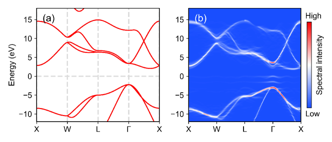
Figure 1: (a) Band structure of diamond in the primitive unit cell. (b) Unfolded band spectrum of the NV center in a supercell.

4.2 Spin texture and Wilson loop

In this example, we demonstrate how to use PYATB to calculate the spin texture and $\mathbb{Z}_{2}$ number for Bi₂Se₃. The $\mathbb{Z}_{2}$ number is a topological invariant that characterizes whether a band insulator with time-reversal symmetry would possess topological properties. In three-dimensional (3D) systems, there are four independent $\mathbb{Z}_{2}$ numbers, consisting of one strong topological index and three weak topological indices. These four $\mathbb{Z}_{2}$ numbers enable the classification of 3D time-reversed band insulators into strong topological insulators, weak topological insulators, and trivial insulators. The Wilson loop method provides a visual means of computing the $\mathbb{Z}_{2}$ number.

Figure 2 depicts the spin texture of Bi₂Se₃ in the $k_{x}$-$k_{y}$ plane for the highest occupied energy band, which is of Rashba-type. Figure 3 shows the Wilson loops of Bi₂Se₃ of the six time-reversal invariant planes in the BZ, which can be used to determine its topological indices ($\nu_{0},\nu_{1}\nu_{2}\nu_{3}$). The results show that the red reference line intersects the Wilson loop an odd number of times at the planes $k_{x}=0$, $k_{y}=0$, and $k_{z}=0$, indicating that the $\mathbb{Z}_{2}$ index is 1. Conversely, for the planes $k_{x}=0.5$, $k_{y}=0.5$, and $k_{z}=0.5$, there is no intersection between the reference line and the Wilson loop, indicating that the $\mathbb{Z}_{2}$ index is 0. Based on these results, we obtain the $\mathbb{Z}_{2}$ topological indices for Bi₂Se₃ as (1,000), confirming that it is a strong topological insulator.

An example Input file for calculating spin textures and Wilson loops using PYATB is provided in A.2.

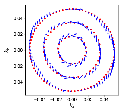
Figure 2: The figure shows the Rashba-type spin texture of the highest occupied energy band in Bi₂Se₃.

Figure 3: Wilson loops for six time-reversal invariant planes of Bi₂Se₃: (a) $k_{x}=0$, (b) $k_{y}=0$, (c) $k_{z}=0$, (d) $k_{x}=0.5$, (e) $k_{y}=0.5$, and (f) $k_{z}=0.5$. The red reference line intersects the Wilson loop an odd number of times for the first three planes, indicating $\mathbb{Z}_{2}=1$, while there is no intersection for the other three planes, indicating $\mathbb{Z}_{2}=0$.

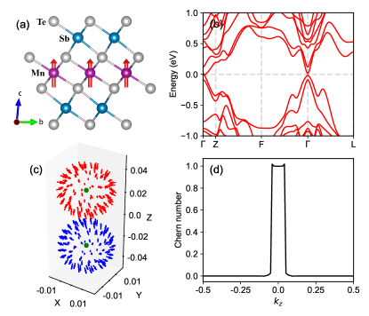
Figure 4: (a) Crystal structure of MnSb₂Te₄. (b) Band structure of MnSb₂Te₄ under FM magnetization. A Weyl point is observed near the Fermi energy on the high symmetry line along $\Gamma-Z$. (c) Two Weyl points in the BZ, as well as the Berry curvature on the spheres surrounding them. The green dots represent the Weyl points, whereas the red and blue arrows indicate the directions of Berry curvature. (d) The Chern number of the $k_{x}-k_{y}$ plane calculated at different $k_{z}$.

4.3 Berry curvature, Chern number, Chirality

MnSb₂Te₄ is a magnetic topological insulator in the antiferromagnetic (AFM) state, but becomes a Weyl semimetal in the ferromagnetic (FM) state [51, 52, 53]. We use the Weyl semimetal state of MnSb₂Te₄ to showcase the capabilities of PYATB, including finding nodes, calculating Berry curvature, Chern number, and chirality functions.

The unit cell of MnSb₂Te₄, consist of septuple layers (SL), is shown in Fig. 4(a) with all spins in Mn atoms aligned in parallel. Figure 4(b) depicts the band structures of MnSb₂Te₄ in the FM state. A band crossing point near the Fermi energy is observed on the $\Gamma-Z$ high symmetry line, which corresponds to a Weyl point. We utilized the find nodes function, and find two band crossing points in the BZ near the Fermi energy. To confirm that they are indeed Weyl points, we calculated the chirality of these two points, and the results are shown in Fig. 4(c). The green dots in Fig. 4(c) represent a pair of Weyl points in the BZ, while the red and blue arrows indicate the direction of Berry curvature on the spheres around the Weyl points. At the Weyl point with $k_{z}>0$, the Berry curvature points inward (red arrows), and the integral over the sphere gives the Chern number (chirality) equal to -1. For the Weyl point with $k_{z}<0$, the Berry curvature points outward (blue arrows), and the chirality equals +1. We further calculated the Chern number of the $k_{x}-k_{y}$ plane at $k_{z}$ and find that the Chern number is 1 between the two Weyl points, and changes abruptly from 1 to 0 upon crossing the Weyl point, as shown in Fig. 4(d).

An example Input file for performing the above-mentioned calculations in PYATB is provided in A.3.

4.4 JDOS, dielectric function

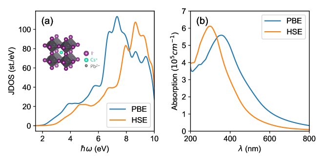
Figure 5: (a) Joint density of states and (b) absorption coefficient of CsPbI₃. The inset figure in (a) depicts the crystal structure of CsPbI₃.

In this example, we calculate the JDOS and optical absorption coefficient of CsPbI₃ using PYATB. CsPbI₃ is an all-inorganic halide perovskite and is considered one of the most promising photovoltaic materials due to its exceptional optoelectronic properties, including a long carrier diffusion length and high photoluminescence (PL) quantum yields [54, 55]. To compare the results, we employed both the Perdew-Burke-Ernzerhof (PBE)[56] functional and the Heyd-Scuseria-Ernzerhof (HSE)[57, 58, 59] hybrid functional in the calculations. The peak position of JDOS in Fig.5(a) obtained using HSE is shifted to the right relative to the PBE peak since PBE tends to underestimate the band gap, while HSE yields more reasonable results. The optical absorption coefficient obtained from HSE also exhibits a blue-shifted onset compared to the PBE one, as shown in Fig.5(b). Furthermore, the HSE spectrum exhibits a strong absorption centered at $\sim$300 nm, consistent with previous theoretical predictions [60].

An example Input file for calculating the joint density of states (JDOS) and optical conductivity is provided in A.4, and the absorption coefficient is calculated using Eq. (53).

4.5 Fat band and shift current

We demonstrate the capabilities of PYATB’s fat band and shift current functions using the WS₂ monolayer as an example. WS₂ is a transition metal dichalcogenide that exhibits a range of intriguing optical properties, such as room temperature photoluminescence and optical Stark effect [61, 62]. In Fig.6(a), we show the fat band structure of WS₂, highlighting the contribution from the W-$5d$ orbital. The red circle sizes in the figure indicate the weight of the $5d$ orbitals. Figure 6(b) illustrates the shift current conductivity of monolayer WS$2$. Since the system has $D_{6h}$ point group symmetry, it has only one independent component $\sigma^{yyy}$. These results are in good agreement with those obtained in Ref. [63].

The Input file for the fat band and shift current calculations is given in the A.5.

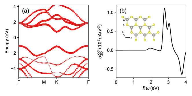
Figure 6: (a) The fat band structure of WS₂ for the W-5$d$ orbital. The size of the red circles represents the weight of the projection. (b) The $yyy$ component of the shift current in WS₂. The inset shows the crystal structure of WS₂.

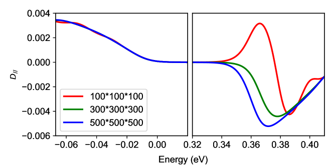
Figure 7: The Berry curvature dipole $D_{//}(E)$($=\frac{1}{2}D_{zz}(E)$) versus energy $E$ measured from the VBM using different $\mathbf{k}$ point meshes.

4.6 Berry curvature dipole

In this example, we showcase the calculation of the Berry curvature dipole of trigonal Te using PYATB. In systems with time-reversal symmetry, a nonlinear anomalous Hall current exists due to a dipole moment induced by the unbalanced distribution of Berry curvature in $\mathbf{k}$-space caused by the breaking of inversion symmetry [46]. The Berry curvature dipole has recently gained attention due to its intriguing topological nature and its potential for photo-electric detections [64, 65].

To begin, we performed ab-initio calculations using the HSE functional implemented in ABACUS to generate the HR, SR, and rR files. We then used PYATB to calculate the Berry curvature dipole of trigonal Te by integrating the entire BZ with meshes of 100$\times$100$\times$100, 300$\times$300$\times$300, and 500$\times$500$\times$500 $\mathbf{k}$ points, respectively. When the Berry curvature at a mesh point exceeds the threshold, we refine the mesh to a size of 20$\times$20$\times$20. The resulting Berry curvature dipoles are shown in Fig.7. Our results suggest that an extremely dense $\mathbf{k}$ points mesh is required to achieve convergence. Specifically, the results obtained with a 300-mesh size are in agreement with those previously reported in the literature using the same $\mathbf{k}$ points mesh [50].

The relevant parameters for calculating the Berry curvature dipole in the Input file are provided in A.6.

5 Summary

The PYATB package is a user-friendly software that allows for the calculation of a broad range of physical properties of materials, such as band structures, associated topological properties, and optical properties. Its most notable advantage is that the ab initio tight-binding Hamiltonian can be naturally generated after the self-consistent calculations using NAO-based first-principles softwares, such as ABACUS, without the need to construct MLWF. This feature simplifies the computational process and ensures the correct symmetry for the systems. We demonstrate the capabilities of PYATB through a few illustrative examples. We hope that PYATB will become a convenient and efficient toolkit for studying the electronic structural properties of materials.

6 Acknowledgments

This work was supported by the Chinese National Science Foundation Grant Number 12134012, and the Innovation Program for Quantum Science and Technology Grant Number 2021ZD0301200. The numerical calculations were performed on the USTC HPC facilities.

Appendix A Example input files

A.1 Input file for NV center

  BANDUNFOLDING  # Specify the purpose of the calculation
  {
      # The STRU file includes the names of the NAO files.
      stru_file     STRU   # The file name for the crystal structure.
      ecut          400    # (eV), the cutoff energy for the plane wave basis of the PC.
      band_range    10 250 # Unfold the 10-th to 250-th bands of the supercell.
      m_matrix      -2 2 2, 2 -2 2, 2 2 -2 # m_ij, i,j = 1, 2, 3
      kpoint_mode   line
      kpoint_num    5    # There are 5 high symmetry k points in the line
      high_symmetry_kpoint
      0.500000  0.000000  0.500000 300  # X, kx, ky, kz, number of k points between X and W
      0.500000  0.250000  0.750000 300  # W
      0.500000  0.500000  0.500000 300  # L
      0.000000  0.000000  0.000000 300  # Gamma
      0.500000  0.000000  0.500000 1    # X
  }

A.2 Input file for Bi₂Se₃

  SPIN_TEXTURE
  {
      nband              78       # Specify the calculated energy band index.
      kpoint_mode        direct   # The k points are given in direct coordinates.
      kpoint_num         140
      kpoint_direct_coor
      0.010000  0.000000 0.000000 # Direct coordinates of the k point
      0.011187  0.003516 0.000000
      0.011279  0.006687 0.000000
      ...
      0.027084 -0.005339 0.000000
      0.028631 -0.002678 0.000000
  }

  WILSON_LOOP
  {
      occ_band      78  # Number of occupied energy bands.
      # To determine a plane of k-space requires an origin (k_start) and
      # two vectors that are not parallel to each other (k_vect1, k_vect2).
      k_start       0.0  0.0  0.5
      k_vect1       1.0  0.0  0.0
      k_vect2       0.0  0.5  0.0
      nk1           101 # number of points of the uniform divide k_vect1.
      nk2           101 # number of points of the uniform divide k_vect2.
  }

A.3 Input file for MnSb₂Te₄

  BAND_STRUCTURE
  {
      kpoint_mode                  line
      kpoint_num                   5
      high_symmetry_kpoint
      # Four numbers, the first three are special k-point coordinates
      # and the fourth is the number of k-points between this
      # special k-point and the next.
      0    0   0    200  # Gamma
      0    0   0.5  200  # Z
      0.5  0   0.5  200  # F
      0    0   0    200  # Gamma
      0.5  0   0    1    # L
  }

  FIND_NODES
  {
      # (eV), search for degenerate k-points with energies
      # in the 9.870 to 10.070 eV range.
      energy_range       9.870 10.070

      # Set the search space of k points.
      # Selecting a parallel hexahedron in k-space requires an
      # origin (k_start) and three vectors (k_vect1, k_vect2, k_vect3)
      # that are not parallel to each other. In this example, k_vect2
      # and k_vect3 are zero vectors, so the chosen search space is
      # k-line from (0.0, 0.0, -0.2) to (0.0, 0.0, 0.4).
      k_start            0.0 0.0 -0.2
      k_vect1            0.0 0.0  0.0
      k_vect2            0.0 0.0  0.0
      k_vect3            0.0 0.0  0.4

      # To start, insert the initial_grid into the search space.
      # Then, check each k-point for its band gap. If the band gap is less than
      # the initial_threshold, refine the k-point using the adaptive_grid located nearby.
      # After refinement, check the band gap of the refined k-point.
      # If it is less than the adaptive_threshold, output the k-point as a result.
      initial_grid       1  1  100
      initial_threshold  0.01  # (eV)
      adaptive_grid      1  1  20
      adaptive_threshold 0.001 # (eV)
  }

  CHIRALITY
  {
      k_vect        0.0000 0.0000 -0.0538 # k coordinates, determine its chirality.
      # unit is 1.0 / angstrom. Draw a spherical surface with the k-point as the
      # center and a radius of 0.02.
      radius        0.02
      point_num     100  # The number of k-points uniformly distributed on the sphere.
  }

  BERRY_CURVATURE
  {
      kpoint_mode                  mp
      # Selecting a parallel hexahedron in k-space requires an
      # origin (k_start) and three vectors (k_vect1, k_vect2, k_vect3)
      # that are not parallel to each other.
      k_start                      0 0 0
      k_vect1                      1 0 0
      k_vect2                      0 1 0
      k_vect3                      0 0 0.5
      # Number of grid points for uniformly dividing 3D k-Space.
      mp_grid                      300 300 50
  }

  CHERN_NUMBER
  {
      occ_band                     109 # Number of occupied energy bands.
      integrate_mode               Grid
      integrate_grid               100 100 1
      # When the Berry curvature of a k point is greater than the
      # threshold (adaptive_grid_threshold), increase the density of k-points
      # around the k point.
      adaptive_grid                20  20  1
      adaptive_grid_threshold      100
      # To determine a plane of k-space requires an origin (k_start) and
      # two vectors that are not parallel to each other (k_vect1, k_vect2).
      k_start                      0 0 0
      k_vect1                      1 0 0
      k_vect2                      0 1 0
  }

A.4 Input file for CsPbI₃

  JDOS
  {
      occ_band      37       # Number of occupied energy bands.
      omega         0.5  10  # (eV), hbar omega.
      domega        0.01     # energy interval.
      eta           0.2      # Gauss smearing parameters.
      grid          30 30 30 # k-space grid points.
  }

  OPTICAL_CONDUCTIVITY #  Calculate the optical conductivity as well as the dielectric functions
  {
      occ_band      37       # Number of occupied energy bands.
      omega         0.5  10  # (eV), hbar omega.
      domega        0.01     # energy interval.
      eta           0.2      # Gauss smearing parameters.
      grid          30 30 30 # k-space grid points.
  }

A.5 Input file for WS₂

  FAT_BAND
  {
      band_range      10 30
      stru_file       STRU    # The file name containing the crystal structure.
      kpoint_mode     line
      kpoint_num      4
      high_symmetry_kpoint
      # Four numbers, the first three are special k-point coordinates
      # and the fourth is the number of k-points between this
      # special k-point and the next.
      0.0000000000   0.0000000000   0.0000000000   20 # GAMMA
      0.5000000000   0.0000000000   0.0000000000   10 # M
      0.3333333333   0.3333333333   0.0000000000   25 # K
      0.0000000000   0.0000000000   0.0000000000   1  # GAMMA
  }

  SHIFT_CURRENT
  {
      occ_band         13     # Number of occupied energy bands.
      omega            0   4  # (eV), hbar omega.
      domega           0.01   # energy interval.
      smearing_method  1 # Gaussian smearing
      eta              0.1    # Gauss smearing parameter
      grid             1000 1000 1 # k-space grid points
  }

A.6 Input file for Te

  BERRY_CURVATURE_DIPOLE
  {
      omega                      9.474 10.074 # (eV) energy range.
      domega                     0.001        # energy interval.
      integrate_mode             Grid
      integrate_grid             500 500 500
      # When the Berry curvature of a k point is greater than the
      # threshold (adaptive_grid_threshold), increase the density of k-points
      # around the k point.
      adaptive_grid              20 20 20
      adaptive_grid_threshold    20000
  }

References

- [1] D. Hsieh, D. Qian, L. Wray, Y. Xia, Y. S. Hor, R. J. Cava, and M. Z. Hasan. A topological dirac insulator in a quantum spin hall phase. Nature, 452(7190):970–974, 2008.
- [2] Haijun Zhang, Chao-Xing Liu, Xiao-Liang Qi, Xi Dai, Zhong Fang, and Shou-Cheng Zhang. Topological insulators in bi2se3, bi2te3 and sb2te3 with a single dirac cone on the surface. Nat. Phys., 5(6):438–442, 2009.
- [3] Y. Xia, D. Qian, D. Hsieh, L. Wray, A. Pal, H. Lin, A. Bansil, D. Grauer, Y. S. Hor, R. J. Cava, and M. Z. Hasan. Observation of a large-gap topological-insulator class with a single dirac cone on the surface. Nat. Phys., 5(6):398–402, 2009.
- [4] Liang Fu. Topological crystalline insulators. Phys. Rev. Lett., 106:106802, Mar 2011.
- [5] Zhijun Wang, Hongming Weng, Quansheng Wu, Xi Dai, and Zhong Fang. Three-dimensional dirac semimetal and quantum transport in cd3as2. Phys. Rev. B, 88:125427, Sep 2013.
- [6] Zhijun Wang, Yan Sun, Xing-Qiu Chen, Cesare Franchini, Gang Xu, Hongming Weng, Xi Dai, and Zhong Fang. Dirac semimetal and topological phase transitions in bi (, k, rb). Phys. Rev. B, 85:195320, May 2012.
- [7] Xiangang Wan, Ari M. Turner, Ashvin Vishwanath, and Sergey Y. Savrasov. Topological semimetal and fermi-arc surface states in the electronic structure of pyrochlore iridates. Phys. Rev. B, 83:205101, May 2011.
- [8] Hongming Weng, Chen Fang, Zhong Fang, B. Andrei Bernevig, and Xi Dai. Weyl semimetal phase in noncentrosymmetric transition-metal monophosphides. Phys. Rev. X, 5:011029, Mar 2015.
- [9] Alexey A. Soluyanov, Dominik Gresch, Zhijun Wang, QuanSheng Wu, Matthias Troyer, Xi Dai, and B. Andrei Bernevig. Type-ii weyl semimetals. Nature, 527(7579):495–498, 2015.
- [10] A. A. Burkov, M. D. Hook, and Leon Balents. Topological nodal semimetals. Phys. Rev. B, 84:235126, Dec 2011.
- [11] Rui Yu, Hongming Weng, Zhong Fang, Xi Dai, and Xiao Hu. Topological node-line semimetal and dirac semimetal state in antiperovskite . Phys. Rev. Lett., 115:036807, Jul 2015.
- [12] Guang Bian, Tay-Rong Chang, Hao Zheng, Saavanth Velury, Su-Yang Xu, Titus Neupert, Ching-Kai Chiu, Shin-Ming Huang, Daniel S. Sanchez, Ilya Belopolski, Nasser Alidoust, Peng-Jen Chen, Guoqing Chang, Arun Bansil, Horng-Tay Jeng, Hsin Lin, and M. Zahid Hasan. Drumhead surface states and topological nodal-line fermions in . Phys. Rev. B, 93:121113, Mar 2016.
- [13] Ming-Che Chang and Qian Niu. Berry curvature, orbital moment, and effective quantum theory of electrons in electromagnetic fields. J. Phys. Condens. Matter, 20(19):193202, apr 2008.
- [14] D. J. Thouless, M. Kohmoto, M. P. Nightingale, and M. den Nijs. Quantized hall conductance in a two-dimensional periodic potential. Phys. Rev. Lett., 49:405–408, Aug 1982.
- [15] Alexey A. Soluyanov and David Vanderbilt. Computing topological invariants without inversion symmetry. Phys. Rev. B, 83:235401, Jun 2011.
- [16] Takahiro Morimoto and Naoto Nagaosa. Topological nature of nonlinear optical effects in solids. Sci. Adv., 2(5):e1501524, 2016.
- [17] Naoto Nagaosa and Takahiro Morimoto. Concept of quantum geometry in optoelectronic processes in solids: Application to solar cells. Adv. Mater., 29(25):1603345, 2017.
- [18] P. Hohenberg and W. Kohn. Inhomogeneous electron gas. Phys. Rev., 136:B864–B871, Nov 1964.
- [19] W. Kohn and L. J. Sham. Self-consistent equations including exchange and correlation effects. Phys. Rev., 140:A1133–A1138, Nov 1965.
- [20] Nicola Marzari, Arash A. Mostofi, Jonathan R. Yates, Ivo Souza, and David Vanderbilt. Maximally localized wannier functions: Theory and applications. Rev. Mod. Phys., 84:1419–1475, Oct 2012.
- [21] Arash A. Mostofi, Jonathan R. Yates, Young-Su Lee, Ivo Souza, David Vanderbilt, and Nicola Marzari. wannier90: A tool for obtaining maximally-localised wannier functions. Comput Phys Commun, 178(9):685–699, 2008.
- [22] et al. Paolo Giannozzi. Quantum espresso: a modular and open-source software project for quantum simulations of materials. J. Phys. Condens. Matter, 21(39):395502, sep 2009.
- [23] G. Kresse and J. Furthmüller. Efficient iterative schemes for ab initio total-energy calculations using a plane-wave basis set. Phys. Rev. B, 54:11169–11186, Oct 1996.
- [24] G. Kresse and J. Furthmüller. Efficiency of ab-initio total energy calculations for metals and semiconductors using a plane-wave basis set. Comput. Mater. Sci., 6(1):15–50, 1996.
- [25] Xavier Gonze, Bernard Amadon, Gabriel Antonius, Frédéric Arnardi, Lucas Baguet, Jean-Michel Beuken, Jordan Bieder, François Bottin, Johann Bouchet, Eric Bousquet, Nils Brouwer, Fabien Bruneval, Guillaume Brunin, Théo Cavignac, Jean-Baptiste Charraud, Wei Chen, Michel Côté, Stefaan Cottenier, Jules Denier, Grégory Geneste, Philippe Ghosez, Matteo Giantomassi, Yannick Gillet, Olivier Gingras, Donald R. Hamann, Geoffroy Hautier, Xu He, Nicole Helbig, Natalie Holzwarth, Yongchao Jia, François Jollet, William Lafargue-Dit-Hauret, Kurt Lejaeghere, Miguel A. L. Marques, Alexandre Martin, Cyril Martins, Henrique P. C. Miranda, Francesco Naccarato, Kristin Persson, Guido Petretto, Valentin Planes, Yann Pouillon, Sergei Prokhorenko, Fabio Ricci, Gian-Marco Rignanese, Aldo H. Romero, Michael Marcus Schmitt, Marc Torrent, Michiel J. van Setten, Benoit Van Troeye, Matthieu J. Verstraete, Gilles Zérah, and Josef W. Zwanziger. The abinit project: Impact, environment and recent developments. Comput. Phys. Commun., 248:107042, 2020.
- [26] Dominik Gresch, Gabriel Autès, Oleg V. Yazyev, Matthias Troyer, David Vanderbilt, B. Andrei Bernevig, and Alexey A. Soluyanov. Z2pack: Numerical implementation of hybrid wannier centers for identifying topological materials. Phys. Rev. B, 95:075146, Feb 2017.
- [27] QuanSheng Wu, ShengNan Zhang, Hai-Feng Song, Matthias Troyer, and Alexey A. Soluyanov. Wanniertools: An open-source software package for novel topological materials. Comput Phys Commun, 224:405–416, 2018.
- [28] Pengfei Li, Xiaohui Liu, Mohan Chen, Peize Lin, Xinguo Ren, Lin Lin, Chao Yang, and Lixin He. Large-scale ab initio simulations based on systematically improvable atomic basis. Comput. Mater. Sci., 112:503–517, 2016. Computational Materials Science in China.
- [29] José M Soler, Emilio Artacho, Julian D Gale, Alberto García, Javier Junquera, Pablo Ordejón, and Daniel Sánchez-Portal. The siesta method for ab initio order-n materials simulation. J. Phys. Condens. Matter, 14(11):2745, mar 2002.
- [30] T. G. Dargam, R. B. Capaz, and Belita Koiller. Disorder and size effects in the envelope-function approximation. Phys. Rev. B, 56:9625–9629, Oct 1997.
- [31] L.-W. Wang, L. Bellaiche, S.-H. Wei, and A. Zunger. “majority representation” of alloy electronic states. Phys. Rev. Lett., 80:4725–4728, May 1998.
- [32] Wei Ku, Tom Berlijn, and Chi-Cheng Lee. Unfolding first-principles band structures. Phys. Rev. Lett., 104:216401, May 2010.
- [33] Voicu Popescu and Alex Zunger. Extracting e versus k effective band structure from supercell calculations on alloys and impurities. Phys. Rev. B, 85:085201, Feb 2012.
- [34] Chi-Cheng Lee, Yukiko Yamada-Takamura, and Taisuke Ozaki. Unfolding method for first-principles lcao electronic structure calculations. J. Phys. Condens. Matter, 25(34):345501, aug 2013.
- [35] Mingxing Chen and M. Weinert. Layer -projection and unfolding electronic bands at interfaces. Phys. Rev. B, 98:245421, Dec 2018.
- [36] Zujian Dai, Gan Jin, and Lixin He. First-principles calculations of the surface states of doped and alloyed topological materials via band unfolding method. Comput. Mater. Sci., 213:111656, 2022.
- [37] J. Zak. Berry’s phase for energy bands in solids. Phys. Rev. Lett., 62:2747–2750, Jun 1989.
- [38] Di Xiao, Ming-Che Chang, and Qian Niu. Berry phase effects on electronic properties. Rev. Mod. Phys., 82:1959–2007, Jul 2010.
- [39] R. D. King-Smith and David Vanderbilt. Theory of polarization of crystalline solids. Phys. Rev. B, 47:1651–1654, Jan 1993.
- [40] Rui Yu, Xiao Liang Qi, Andrei Bernevig, Zhong Fang, and Xi Dai. Equivalent expression of topological invariant for band insulators using the non-abelian berry connection. Phys. Rev. B, 84:075119, Aug 2011.
- [41] Xifan Wu, Oswaldo Diéguez, Karin M. Rabe, and David Vanderbilt. Wannier-based definition of layer polarizations in perovskite superlattices. Phys. Rev. Lett., 97:107602, Sep 2006.
- [42] Alexey A. Soluyanov and David Vanderbilt. Wannier representation of topological insulators. Phys. Rev. B, 83:035108, Jan 2011.
- [43] Gan Jin, Daye Zheng, and Lixin He. Calculation of berry curvature using non-orthogonal atomic orbitals. J. Phys. Condens. Matter, 33(32):325503, jun 2021.
- [44] Chi-Cheng Lee, Yung-Ting Lee, Masahiro Fukuda, and Taisuke Ozaki. Tight-binding calculations of optical matrix elements for conductivity using nonorthogonal atomic orbitals: Anomalous hall conductivity in bcc fe. Phys. Rev. B, 98:115115, Sep 2018.
- [45] Boris I Sturman and Vladimir M Fridkin. The Photovoltaic and Photorefractive Effects in Noncentrosymmetric Materials. Gordon and Breach Science Publishers, 1 edition, 1992.
- [46] J. E. Sipe and A. I. Shkrebtii. Second-order optical response in semiconductors. Phys. Rev. B, 61:5337–5352, Feb 2000.
- [47] Julen Ibañez Azpiroz, Stepan S. Tsirkin, and Ivo Souza. Ab initio calculation of the shift photocurrent by wannier interpolation. Phys. Rev. B, 97:245143, Jun 2018.
- [48] Inti Sodemann and Liang Fu. Quantum nonlinear hall effect induced by berry curvature dipole in time-reversal invariant materials. Phys. Rev. Lett., 115:216806, Nov 2015.
- [49] Yang Zhang and Liang Fu. Terahertz detection based on nonlinear hall effect without magnetic field. Proc. Nat. Acad. Sci., 118(21):e2100736118, 2021.
- [50] Stepan S. Tsirkin, Pablo Aguado Puente, and Ivo Souza. Gyrotropic effects in trigonal tellurium studied from first principles. Phys. Rev. B, 97:035158, Jan 2018.
- [51] J.-Q. Yan, S. Okamoto, M. A. McGuire, A. F. May, R. J. McQueeney, and B. C. Sales. Evolution of structural, magnetic, and transport properties in . Phys. Rev. B, 100:104409, Sep 2019.
- [52] Stefan Wimmer, Jaime Sánchez-Barriga, Philipp Küppers, Andreas Ney, Enrico Schierle, Friedrich Freyse, Ondrej Caha, Jan Michalička, Marcus Liebmann, Daniel Primetzhofer, Martin Hoffman, Arthur Ernst, Mikhail M. Otrokov, Gustav Bihlmayer, Eugen Weschke, Bella Lake, Evgueni V. Chulkov, Markus Morgenstern, Günther Bauer, Gunther Springholz, and Oliver Rader. Mn-rich mnsb2te4: A topological insulator with magnetic gap closing at high curie temperatures of 45–50 k. Adv. Mater., 33(42):2102935, 2021.
- [53] Gang Shi, Mingjie Zhang, Dayu Yan, Honglei Feng, Meng Yang, Youguo Shi, and Yongqing Li. Anomalous hall effect in layered ferrimagnet mnsb2te4*. Chinese Phys. Lett., 37(4):047301, apr 2020.
- [54] Subham Dastidar, Siming Li, Sergey Y. Smolin, Jason B. Baxter, and Aaron T. Fafarman. Slow electron–hole recombination in lead iodide perovskites does not require a molecular dipole. ACS Energy Lett., 2(10):2239–2244, 2017.
- [55] Qiang Jing, Mian Zhang, Xiang Huang, Xiaoming Ren, Peng Wang, and Zhenda Lu. Surface passivation of mixed-halide perovskite cspb(brxi1-x)3 nanocrystals by selective etching for improved stability. Nanoscale, 9(22):7391–7396, 2017.
- [56] John P. Perdew, Kieron Burke, and Matthias Ernzerhof. Generalized gradient approximation made simple. Phys. Rev. Lett., 77:3865–3868, Oct 1996.
- [57] Jochen Heyd, Gustavo E. Scuseria, and Matthias Ernzerhof. Hybrid functionals based on a screened coulomb potential. J. Chem. Phys., 118(18):8207–8215, 2003.
- [58] Jochen Heyd, Gustavo E. Scuseria, and Matthias Ernzerhof. Erratum: “hybrid functionals based on a screened coulomb potential” [j. chem. phys. 118, 8207 (2003)]. J. Chem. Phys., 124(21):219906, 2006.
- [59] Aliaksandr V. Krukau, Oleg A. Vydrov, Artur F. Izmaylov, and Gustavo E. Scuseria. Influence of the exchange screening parameter on the performance of screened hybrid functionals. J. Chem. Phys., 125(22):224106, 2006.
- [60] Diwen Liu, Wenying Zha, Yongmei Guo, and Rongjian Sa. Insight into the improved phase stability of cspbi3 from first-principles calculations. ACS Omega, 5(1):893–896, 2020.
- [61] Humberto R. Gutiérrez, Nestor Perea-López, Ana Laura Elías, Ayse Berkdemir, Bei Wang, Ruitao Lv, Florentino López-Urías, Vincent H. Crespi, Humberto Terrones, and Mauricio Terrones. Extraordinary room-temperature photoluminescence in triangular ws2 monolayers. Nano Lett., 13(8):3447–3454, 2013.
- [62] Edbert J. Sie, James W. McIver, Yi-Hsien Lee, Liang Fu, Jing Kong, and Nuh Gedik. Valley-selective optical stark effect in monolayer ws2. Nat. Mater., 14(3):290–294, 2015.
- [63] Chong Wang, Sibo Zhao, Xiaomi Guo, Xinguo Ren, Bing-Lin Gu, Yong Xu, and Wenhui Duan. First-principles calculation of optical responses based on nonorthogonal localized orbitals. New J. Phys., 21(9):093001, sep 2019.
- [64] Z. Z. Du, C. M. Wang, Hai-Peng Sun, Hai-Zhou Lu, and X. C. Xie. Quantum theory of the nonlinear hall effect. Nat. Commun., 12(1):5038, 2021.
- [65] Qiong Ma, Su-Yang Xu, Huitao Shen, David MacNeill, Valla Fatemi, Tay-Rong Chang, Andrés M. Mier Valdivia, Sanfeng Wu, Zongzheng Du, Chuang-Han Hsu, Shiang Fang, Quinn D. Gibson, Kenji Watanabe, Takashi Taniguchi, Robert J. Cava, Efthimios Kaxiras, Hai-Zhou Lu, Hsin Lin, Liang Fu, Nuh Gedik, and Pablo Jarillo-Herrero. Observation of the nonlinear hall effect under time-reversal-symmetric conditions. Nature, 565(7739):337–342, 2019.