The modelling error in multi-dimensional time-dependent solute transport models

Abstract.

Starting from full-dimensional models of solute transport, we derive and analyze multi-dimensional models of time-dependent convection, diffusion, and exchange in and around pulsating vascular and perivascular networks. These models are widely applicable for modelling transport in vascularized tissue, brain perivascular spaces, vascular plants and similar environments. We show the existence and uniqueness of solutions to both the full- and the multi-dimensional equations under suitable assumptions on the domain velocity. Moreover, we quantify the associated modelling errors by establishing a-priori estimates in evolving Bochner spaces. In particular, we show that the modelling error decreases with the characteristic vessel diameter and thus vanishes for infinitely slender vessels. Numerical tests in idealized geometries corroborate and extend upon our theoretical findings.

Key words. Multi–dimensional modeling; time dependent convection–diffusion, solute transport models; modeling error in evolving Bochner spaces.

AMS Subject Classification. 35K45, 65G99, 65J08, 65M15, 92-10.

1. Introduction

We consider transport of solutes by diffusion, convection, and exchange in a coupled system consisting of networks of slender vessels and their surroundings. This setting is ubiquitous in the human body [5] as exemplified by the transport and exchange of nutrients such as oxygen or glucose, or medical drugs in the vasculature and surrounding tissue, e.g. in skeletal muscle, the liver [52], or the placenta [61]; or conversely, the transport of metabolic by-products from tissue into and through lymphatic vessels [50]. Similar structures and processes are also fundamental in biology, think of e.g. the roots of vascularized plants [32], and in geoscience e.g. in connection with flow and transport in reservoir wells [21], in the context of C02 sequestration [48], or groundwater contamination [43].

Of particular interest, both from a physiological and mathematical point-of-view, is the transport of solutes in, around and out of the human brain. Despite decades – even centuries – of research, solute transport and clearance within the human brain remain poorly understood [62, 27, 29]. In contrast to the rest of the body, the brain vasculature is equipped with a blood-brain-barrier, which carefully regulates the exchange of substances between the blood and the surrounding tissue, while the brain parenchyma itself lacks typical lymph vessels. Better understanding of these physiological processes is vital for targeting brain drug delivery [45, 42] or for unraveling the role of metabolic waste clearance in neurodegenerative disease [56, 29]. Concurrently, in tissue engineering, efforts are currently underway to develop human brain cortical organoids, but crucially rely on vascularization via e.g. microfluidic devices for improved oxygen and nutrient transport as well as cellular signalling [39].

The human brain is composed of soft tissue, is lined and penetrated by networks of blood vessels, and is surrounded by the narrow subarachnoid space filled with cerebrospinal fluid (CSF). The cerebral arteries pulsate in sync with the cardiac cycle and undergo other forms of vasomotion with variations in radii of $\sim$1–10% [44], while the entire brain parenchyma deforms by around 1% as the result of a complex interplay between the cardiac and respiratory cycles as well as autoregulation [54, 10]. Perivascular (or paravascular) spaces (PVSs) are spaces surrounding the vasculature on the brain surface or within the brain parenchyma. On the brain surface, these spaces are clearly visible [58], and PVSs persist as the blood vessels branch and penetrate into the brain parenchyma – then known as Virchow-Robin spaces. The extent to which perivascular spaces exist along the length of the vasculature within the brain, even to the capillary level, is debated however [25]. Within the parenchyma, perivascular spaces are often represented as generalized (elliptic) annular cylinders, filled with cerebrospinal or interstitial fluid and bounded by a nearly tight layer of astrocyte endfeet, see e.g. [8, 60, 15] and references therein.

Solutes move by diffusion within the brain tissue [46], and by diffusion and convection within the vasculature [5]. However, to what extent also convection in perivascular, intracellular or extracellular spaces play a role in brain solute transport and clearance stand as important open questions. Convective velocity magnitudes are expected to differ by many orders of magnitude between and within the respective compartments: blood may flow at the order of 1 m/s in major cerebral arteries [5], CSF flows in surface perivascular spaces at up to 60 $\mu$m/s with Péclet numbers of up to 1000 [44], while flow of interstitial fluid within the tissue is unlikely to exceed 10 $\mu$m/min on average [59, 1]. Depending on their ability to cross the blood-brain barrier, solutes may also exchange between the vascular and perivascular spaces, as well as into the surrounding tissue or subarachnoid space. To mathematically and computationally study such transport at the scale of larger vascular networks, our target here is to derive and analyze time-dependent convection-diffusion models with a geometrically-explicit but dimensionally-reduced representation of the (peri)vascular spaces coupled with the full-dimensional surroundings.

As a starting point (more precise details are presented later), consider second-order elliptic equations describing diffusion of the solute concentrations $c_{v}:\Omega_{v}\rightarrow\mathbb{R}$, and $c_{s}:\Omega_{s}\rightarrow\mathbb{R}$:

(1.1a) $$-\nabla\cdot D\nabla c_{s} =f\quad\text{ in }\Omega_{s},$$

(1.1b) $$-\nabla\cdot D\nabla c_{v} =f\quad\text{ in }\Omega_{v},$$

where $D$ is a given effective diffusion coefficient and $f$ given sources. Assuming that the compartments are separated by a semi-permeable membrane $\Gamma$ gives the interface condition

(1.2) $$D\nabla c\cdot\boldsymbol{n}=\xi[[c]]\quad\text{ on }\Gamma,$$

where $\boldsymbol{n}$ is the interface normal, $[[\cdot]]$ denotes the jump across the interface(s), and $\xi$ is a membrane permeability parameter. Now assuming that $\Omega_{v}$ can be well-represented by its centerline $\Lambda$ with coordinate $s$ (to be made more precise later), the coupled 3D-3D problem of (1.1)–(1.2) may be reduced to a coupled 3D-1D problem of the form: find the solute concentrations $\bar{c}:\Lambda\rightarrow\mathbb{R}$, and $c:\Omega\rightarrow\mathbb{R}$

(1.3a) $$-\nabla\cdot D\nabla c+\mathcal{C}=f\quad\text{ in }\Omega,$$

(1.3b) $$-\partial_{s}\bar{D}\partial_{s}\bar{c}+\bar{\mathcal{C}}=\bar{f}\quad\text{ on }\Lambda,$$

where $\mathcal{C}$, $\bar{\mathcal{C}}$ denote coupling terms depending on the concentrations $c,\bar{c}$, and choice of coupling. Note that flow in a porous medium (Darcy flow) can be described with the same equation structure, with $c$ instead representing the pore pressure and $D$ the hydraulic conductance. Modelling, discretization, and applications of 3D-1D problems such as (1.3) has been the subject of active research, especially over the last two decades, with key contributions from e.g. [19, 13, 12, 49, 34, 22, 37, 31, 36] and references therein to mention but a few. Notably, Laurino and Zunino [40] rigorously analyze the modelling error associated with replacing (1.1)–(1.2) by (1.3), and demonstrate that the modelling error indeed vanishes for infinitely thin vessels.

Here, we consider a parabolic extension of the classical elliptic 3D-1D equations (1.3) accounting also for (i) time-evolving distributions, (ii) convective transport, (iii) moving interfaces, and (iv) both cylindrical and non-convex (annular) vessel networks representing e.g. vascular and perivascular spaces, respectively. We also derive and study a 3D-1D-1D model representing solute transport in coupled tissue, perivascular and vascular spaces. Previously, Possenti, Zunino and coauthors [51] and Köppl, Vidotto and Wohlmuth [33] have studied applications of 3D-1D models for (oxygen) transport including convection but at steady state. Furthermore, Formaggia et al [20] consider coupled Navier–Stokes equations for flow problems in compliant vessels but with a different type of mixed-dimensional coupling. More specifically, we are interested in solute concentrations $c_{v}(t):\Omega_{v}(t)\rightarrow\mathbb{R}$, and $c_{s}(t):\Omega_{s}(t)\rightarrow\mathbb{R}$ satisfying the time-dependent diffusion equations for a.e. $t>0$:

(1.4a) $$\partial_{t}c_{s}+\boldsymbol{u}\cdot\nabla c_{s}-\nabla\cdot D\nabla c_{s} =f\quad\text{ in }\Omega_{s}(t),$$

(1.4b) $$\partial_{t}c_{v}+\boldsymbol{u}\cdot\nabla c_{v}-\nabla\cdot D\nabla c_{v} =f\quad\text{ in }\Omega_{v}(t),$$

where now additionally $\boldsymbol{u}$ represents a convective velocity field and the interface $\Gamma$ between $\Omega_{s}$ and $\Omega_{t}$ is allowed to move and deform in time.

Our main findings are as follows.

• We introduce a system of time-dependent convection-diffusion equations in and around embedded networks of moving vessels. Under suitable assumptions on the domain velocity, we prove well-posedness i.e. that suitably regular weak solutions to these equations exist and are unique (Section 3).

• We derive reduced 1D equations, and we formally derive weak formulations of 3D-1D and 3D-1D-1D coupled models of time-dependent solute transport governed by convection, diffusion, and exchange in deforming vascular and/or perivascular networks, and the surrounding domain (Section 4, Section 5). We prove well-posedness of the coupled 3D-1D formulation and show a regularity estimate for the 3D solution. These formulations are widely applicable for modelling transport in vascularized tissue in general and the brain in particular, vascular plant environments etc.

• We rigorously estimate the modelling error in evolving Bochner spaces associated with replacing the time-dependent 3D-3D convection-diffusion problem by the 3D-1D problem via a duality argument. We show that a relevant dual problem is well-posed, and that the modelling error decreases with the characteristic vessel diameter $\epsilon$, and thus vanishes as $\epsilon\rightarrow 0$ (Section 7).

• The presence of deforming networks with annular cross-sections poses key technical challenges relating to classical numerical analysis tools, such as e.g. Poincaré and trace inequalities, and extension operators over moving, non-convex domains, which we address separately (Section 6).

These points are prefaced by introducing notation and preliminary results in Section 2, while concluding remarks and outlook relating to e.g. the discretization errors form Section 9.

2. Notation and preliminaries

2.1. Function spaces, inner products and norms

Given an open domain $O\subset\mathbb{R}^{d}$, $d\in\{1,2,3\}$ and measurable real valued functions $f,g$ , we let $(f,g)_{O}$ denote the usual $L^{2}$ inner product. If $O$ is the whole domain $\Omega$, the we write $(f,g)=(f,g)_{\Omega}$. The Hilbert space gernerated by this inner product is denoted by $L^{2}(O)$ with the usual induced norm $\|\cdot\|_{L^{2}(O)}$. We also use standard notation for the Sobolev spaces $W^{m,p}(O)$ and $H^{m}(O)=W^{m,2}(O)$ for $m\in\mathbb{N}$ and $1\leq p\leq\infty$. For a given weight $w\in L^{\infty}(O)$ and $w>0$ a.e. in $O$, we define the weighted $L^{2}$ inner product $(f,g)_{O,w}=(f,wg)_{O}$ and the respective weighted $L^{2}$ space :

(2.1) $$\|f\|_{L^{2}_{w}(O)}=\|w^{1/2}f\|_{L^{2}(O)},\,\,L^{2}_{w}(O)=\{f:O\rightarrow\mathbb{R}\,\,|\,\,\|f\|_{L_{w}^{2}(O)}<\infty\}.$$

The weighted Sobolev space $H^{1}_{w}(O)$ is then defined as

(2.2) $$H^{1}_{w}(O)=\{f\in L^{2}_{w}(O)\,\,|\,\,\|\nabla f\|_{L^{2}_{w}(O)}<\infty\},$$

and the weighted inner product and norm are

(2.3) $$(f,g)_{H^{1}_{w}(O)}=(f,g)_{L^{2}_{w}(O)}+(\nabla f,\nabla g)_{L^{2}_{w}(O)},\,\,\,\|f\|_{H^{1}_{w}(O)}^{2}=\|f\|_{L^{2}_{w}(O)}^{2}+\|\nabla f\|_{L^{2}_{w}(O)}^{2}.$$

We omit the subscript/weight $w$ when $w=1$.

Given a Hilbert space $X$, we denote the dual space of $X$ by $X^{\prime}$. The duality pairing between $X$ and $X^{\prime}$ is denoted by

$$\langle v^{\prime},v\rangle_{X^{\prime}\times X}.$$

For brevity in notation, we let

$$H^{-1}_{w}(O)=H_{w}^{1}(O)^{\prime},\qquad\langle v^{\prime},v\rangle_{H^{-1}_{w}(O)}=\langle v^{\prime},v\rangle_{H^{-1}_{w}(O)\times H^{1}_{w}(O)}.$$

We also recall the definition of standard Bochner type spaces. For $t,T>0$, $f:(t,T)\rightarrow X$, we say that $f\in L^{2}(t,T;X)$ if

(2.4) $$\|f\|^{2}_{L^{2}(t,T;X)}=\int_{t}^{T}\|f\|_{X}^{2}<\infty.$$

If $f$ is weakly differentiable in time and $\partial_{t}f\in L^{2}(t,T;X)$, then we say $f\in H^{1}(t,T;X)$ with the norm:

(2.5) $$\|f\|_{H^{1}(t,T;X)}^{2}=\|f\|_{L^{2}(t,T;X)}^{2}+\|\partial_{t}f\|_{L^{2}(t,T;X)}^{2}.$$

Given two Hilbert spaces $V$ and $H$ with $V\subset H$, we define

(2.6) $$\mathcal{W}(V,H)=\{v:(0,T)\rightarrow V;v\in L^{2}(0,T;V),\,\,\partial_{t}v\in L^{2}(0,T;H)\}.$$

Finally, we will use the space $C^{0}(0,T;V)$ of continuous $V$-valued functions and the space $\mathcal{D}(0,T;V)$ of infinitely differentiable $V$-valued functions.

2.2. The geometrical setting

We consider a generalized annular domain $\Omega_{v}$ (Figure 1), described in cylindrical coordinates and moving in time:

$$\Omega_{v}(t)=\{\boldsymbol{\lambda}(s)+r\cos(\theta)\boldsymbol{N}(s)+r\sin(\theta)\boldsymbol{B}(s),\\ 0<s<L,\,0\leq\theta\leq 2\pi,\,R_{1}(s,t,\theta)<r<R_{2}(s,t,\theta)\}\subset\mathbb{R}^{3}$$

of length $L>0$, inner radius $R_{1}\geqslant 0$, and outer radius $R_{2}>0$. We refer to the $s$-direction as the axial direction. For $R_{1}=0$, we consider a cylindrical domain where in the above definition, we let $0\leq r<R_{2}(s,t,\theta)$. In general, $\Omega_{v}$ represents a vessel segment such as a perivascular space ($R_{1}>0$), or blood vessel segment, plant root or borehole ($R_{1}=0$). We assume that $\boldsymbol{\lambda}(s)=[\lambda^{1}(s),\lambda^{2}(s),\lambda^{3}(s)]$ above is a parametrized $C^{2}$-regular curve with non-moving centerline $\Lambda$ defined as $\Lambda=\{\boldsymbol{\lambda}(s)\}$ for $s\in(0,L)$, and that $\|\boldsymbol{\lambda}^{\prime}(s)\|=1$, thus implying that $s$ is the arc length. The vectors $\boldsymbol{N}$ and $\boldsymbol{B}$ are from the Frenet-Serret frame of $\Lambda$. Throughout the paper, $\Theta(s,t)$ denotes the cross-section of $\Omega_{v}(t)$ at $s\in\Lambda$.

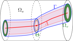
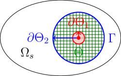
Figure 1. Geometrical setting. Left: An (annular) cylinder $\Omega_{v}$ (shown in green) representing a vessel parametrized in terms of the centerline curve $\Lambda$ (shown in red). The vessel is surrounded by the domain $\Omega_{s}$ while $\Gamma$ forms the lateral boundary between the domains (shown in blue). Right: Lateral cross-section of the domain $\Omega$ showing $\Omega_{v}$ in green, the inner boundary $\partial\Theta_{1}$ in red, and the outer boundary $\partial\Theta_{2}$ or $\Gamma$ in blue. Note that in the annular cylinder case, the inner-most cylinder, i.e. the extrusion along $\Lambda$ of the domain bounded by $\partial\Theta_{1}$, is not part of $\Omega_{s}$ or $\Omega_{v}$.

This domain $\Omega_{v}(t)$ is embedded into a fixed domain $\Omega\subset\mathbb{R}^{3}$ with (outer) surroundings $\Omega_{s}=\Omega\backslash B_{R_{2}}$ where $B_{R_{2}}$ is the outer cylinder given by:

$$B_{R_{2}}(t)=\{\boldsymbol{\lambda}(s)+r\cos(\theta)\boldsymbol{N}(s)+r\sin(\theta)\boldsymbol{B}(s),\\ 0<s<L,\,0\leq\theta\leq 2\pi,\,0\leq r<R_{2}(s,t,\theta)\}.$$

We emphasize that, by construction, the surrounding domain $\Omega_{s}$ does not include the vessel $\Omega_{v}$ itself nor the inner-most generalized cylinder in the case $R_{1}>0$. We assume that for all $t\in[0,T]$, $\Omega_{v}(t)$ is completely embedded in $\Omega$; that is,

$$\mathrm{dist}(\partial\Omega_{v}(t),\partial\Omega)>0,\quad\forall t\in[0,T].$$

We denote by $\Gamma$ the lateral boundary of $\Omega_{v}$ intersecting the boundary of $\Omega_{s}(t)$, $\Gamma=\partial\Omega_{v}\cap\partial\Omega_{s}$, and by $\Gamma_{0}$ and $\Gamma_{L}$ the vertical boundary of $\Gamma$ at $s=0$ and at $s=L$ respectively. The unit normal to $\partial\Omega_{v}$ is denoted by $\boldsymbol{n}_{v}$, and on $\Gamma$, $\boldsymbol{n}_{s}=-\boldsymbol{n}_{v}$. For each cross-section $\Theta(s,t)$, we label its area $A(s,t)=|\Theta(s,t)|$ for $s\in\Lambda$ and $t\in[0,T]$. We also label the boundary of the lateral cross-section of $\Theta$ by $\partial\Theta$, the boundary of the outer circle (at $r=R_{2}$) by $\partial\Theta_{2}$, and (if $R_{1}>0$) the boundary of the inner circle (at $r=R_{1}$) by $\partial\Theta_{1}$. We denote by $P(s,t)=|\partial\Theta_{2}(s,t)|$ the perimeter of the outer circle (representing the interface between the vessel and its outer surroundings).

Note that we consider vessels $\Omega_{v}$ both of cylinder-type or annular cylinder-type and their (outer) surroundings. The former case is well-suited to represent e.g. transport in the vasculature, roots or geothermal wells. The latter case targets e.g. perivascular transport in the brain, intracranial space, or spinal compartments. In the latter (annular cylinder) case, we only include the outer surroundings in the 3D-3D and reduced 3D-1D model formulations in the subsequent Sections 3–4. The distinction between inner and outer surroundings are motivated by the potentially large jumps in material parameters such as the convective velocity or diffusion coefficient between the inner and outer compartments in applications. Such jumps would be challenging to represent in an extended domain in the 3D-1D setting. These models are thus particularly relevant for perivascular transport with a vascular-perivascular barrier, such as e.g. the blood-brain barrier (BBB) in the human brain. However, the case of vascular-perivascular exchange may also be highly relevant e.g. in connection with a leaky BBB or transport of substances across the BBB. Therefore, we address the extended 3D-3D-3D and 3D-1D-1D problem setting representing coupled tissue, perivascular and vascular transport separately in Section 5.

In Section 4.6, we will also consider an extension of this setting to networks of vessels. We will then consider a network of $N$ domains $\Omega_{v,i}$ with center-curves $\Lambda_{i}=\{\boldsymbol{\lambda}_{i}(s),\,\,s\in(0,L_{i})\}$ for $i=1,\ldots,N$. Extending upon the notation introduced above, we then denote $A_{i}=|\Theta_{i}|$ and $P_{i}=|\partial\Theta_{2,i}|$ where $\Theta_{i}$ is the cross-section of $\Omega_{v,i}$ and $\partial\Theta_{2,i}$ is the outer boundary of $\Omega_{v,i}$.

3. Transport by convection and diffusion in a moving domain

We are interested in analyzing the coupled transport of a solute in a moving domain governed by diffusion and convection in general, and in a moving vessel and its surroundings in particular. To this end, we introduce a system of coupled convection-diffusion equations (Section 3.1). We may directly consider a more general geometrical setting (Section 3.2) for the weak formulation (Section 3.3) to show that such solutions exist (Section 3.4, 3.1).

3.1. System of convection-diffusion equations in and around a moving vessel

We consider a moving vessel and assume that the vessel motion $\Omega_{v}(t)$, and convective velocity fields $\boldsymbol{u}_{v}(t):\Omega_{v}\rightarrow\mathbb{R}^{3}$ and $\boldsymbol{u}_{s}(t):\Omega_{s}\rightarrow\mathbb{R}^{3}$ are prescribed for $t\in[0,T]$. Our coupled three-dimensional transport boundary-value problem in an Eulerian frame reads as: for a.e. $t$, find the solute concentrations $c_{v}(t):\Omega_{v}(t)\rightarrow\mathbb{R}$ and $c_{s}(t):\Omega_{s}(t)\rightarrow\mathbb{R}$ such that the following governing equations, interface conditions, boundary conditions and initial conditions hold:

(3.1a) $$\partial_{t}c_{v}-\nabla\cdot(D_{v}\nabla c_{v})+\nabla\cdot(\boldsymbol{u}_{v}c_{v}) =f_{v}, \quad\mathrm{in}\,\Omega_{v}(t)\times(0,T],$$

(3.1b) $$\partial_{t}c_{s}-\nabla\cdot(D_{s}\nabla c_{s})+\nabla\cdot(\boldsymbol{u}_{s}c_{s}) =f_{s}, \quad\mathrm{in}\,\Omega_{s}(t)\times(0,T],$$

(3.1c) $$(c_{v}\tilde{\boldsymbol{u}}_{v}-D_{v}\nabla c_{v})\cdot\boldsymbol{n}_{v}-\xi(c_{v}-c_{s}) =0, \quad\mathrm{on}\,\Gamma(t)\times(0,T],$$

(3.1d) $$(c_{v}\tilde{\boldsymbol{u}}_{v}-D_{v}\nabla c_{v})\cdot\boldsymbol{n}_{v}+(c_{s}\tilde{\boldsymbol{u}}_{s}-D_{s}\nabla c_{s})\cdot\boldsymbol{n}_{s} =0, \quad\mathrm{on}\,\Gamma(t)\times(0,T],$$

(3.1e) $$(c_{v}\tilde{\boldsymbol{u}}_{v}-D_{v}\nabla c_{v})\cdot\boldsymbol{n}_{v}=(c_{s}\tilde{\boldsymbol{u}}_{s}-D_{s}\nabla c_{s})\cdot\boldsymbol{n}_{s} =0, \quad\mathrm{on}\,(\Gamma_{0}(t)\cup\Gamma_{L}(t))\times(0,T],$$

(3.1f) $$c_{s} =0, \quad\mathrm{on}\,\partial\Omega\times(0,T],$$

(3.1g) $$c_{v}(0)=c_{v}^{0},\quad\mathrm{in}\,\Omega_{v}(0),\quad c_{s}(0) =c_{s}^{0} \quad\mathrm{in}\,\Omega_{s}(0).$$

If $\partial\Omega_{v}\backslash\Gamma\neq\emptyset$ $(R_{1}>0$, an annular domain $\Omega_{v}$), we also impose the boundary condition:

(3.2) $$(c_{v}\tilde{\boldsymbol{u}}_{v}-D_{v}\nabla c_{v})\cdot\boldsymbol{n}_{v} =0 \quad\mathrm{on}\,\partial\Omega_{v}(t)\backslash\Gamma(t)\times(0,T].$$

The time derivatives in the above formulation are the Eulerian time derivatives. The parameters $D_{v}$, $D_{s}$ are given diffusion tensors in $\Omega_{v}$ and $\Omega_{s}$ respectively, while $f_{v}$ and $f_{s}$ are given source functions. For $i\in\{v,s\}$, the relative (net) velocity $\tilde{\boldsymbol{u}}_{i}=\boldsymbol{u}_{i}-\boldsymbol{w}$ accounts for the velocity of the domain $\boldsymbol{w}$, defined below cf. (3.3). The interface condition (3.1c) models the lateral interface between the vessel and its surroundings $\Gamma$ as a semi-permeable membrane with permeability $\xi$, while the auxiliary condition (3.1d) enforces conservation of mass. At the vertical boundaries, the condition (3.1e) stipulates no flux, while we keep the concentration fixed and zero (for simplicity) at the outermost boundary $\partial\Omega$ via (3.1f). The last relations (3.1g) define the initial conditions with given initial states $c_{v}^{0}:\Omega_{v}\rightarrow\mathbb{R},\,c_{v}^{0}\in L^{2}(\Omega_{v})$ and $c_{s}^{0}:\Omega_{s}\rightarrow\mathbb{R},\,c_{s}^{0}\in L^{2}(\Omega_{s})$.

3.2. Observations on the domain velocity

For the existence result we can weaken our geometrical assumptions on the domains. Precisely, we let $\Omega(0)\subset\mathbb{R}^{d}$ be a Lipschitz domain, i.e., open, connected and with a Lipschitz boundary and we assume that $\Omega_{v}(0)\subset\Omega(0)$ is itself a Lipschitz domain and compactly contained in $\Omega(0)$. In particular, it holds $\operatorname{dist}(\partial\Omega_{v}(0),\partial\Omega(0))>0$. We measurably partition $\partial\Omega_{v}(0)$ into two sets that play the role of $\Gamma(0)$ in (3.1c) and (3.1d) and $\Gamma_{0}(0)\cup\Gamma_{L}(0)$ in (3.1e), respectively (and will be denoted by the same symbols).

We define moving domains according to the velocity method, see [16]. More precisely, assume that the domain velocity $\boldsymbol{w}:\mathbb{R}^{d}\times\mathbb{R}\to\mathbb{R}^{d}$ is smooth and compactly supported. We denote by $\boldsymbol{\psi}:\mathbb{R}^{d}\times\mathbb{R}\to\mathbb{R}^{d}$ the flow map of the order

(3.3) $$\begin{split}\partial_{t}\boldsymbol{\psi}(\boldsymbol{x},t)&=\boldsymbol{w}(\boldsymbol{\psi}(\boldsymbol{x},t),t),\\ \boldsymbol{\psi}(\boldsymbol{x},0)&=\boldsymbol{x}.\end{split}$$

Standard ODE theory implies that $\boldsymbol{\psi}\in C^{\infty}(\mathbb{R}^{d+1})$ and for all fixed $t\in[0,T]$ the map

$$\boldsymbol{\psi}_{t}:\mathbb{R}^{d}\to\mathbb{R}^{d},\quad\boldsymbol{x}\mapsto\boldsymbol{\psi}(\boldsymbol{x},t)$$

is a diffeomorphism. In this notation, the connection between our reference domain and the domains to a later time is given by

$$\Omega_{s}(t)=\boldsymbol{\psi}_{t}(\Omega_{s}(0)),\quad\Omega_{v}(t)=\boldsymbol{\psi}_{t}(\Omega_{v}(0)).$$

As $\Omega_{s}(0)$ and $\Omega_{v}(0)$ are open, connected and Lipschitz it holds $\partial\Omega_{v}(t)=\boldsymbol{\psi}_{t}(\partial\Omega_{v}(0))$ and $\partial\Omega_{v}(t)$ has Lipschitz boundary, see [28]. An important observation which links the above definitions to the specific setting in subsection 2.2 is now in order. Denoting by $\mathrm{det}(D\boldsymbol{\psi}_{t})$ the determinant of the Jacobian matrix of $\boldsymbol{\psi}_{t}$, it holds that [47, Section 1.1.1]:

(3.4) $$\partial_{t}A(s,t)=\partial_{t}\int_{\Theta(s,t)}1=\partial_{t}\int_{\Theta(s,0)}|\mathrm{det}(D\boldsymbol{\psi}_{t})|\\ =\int_{\Theta(s,0)}\boldsymbol{\psi}_{-t}(\nabla\cdot\boldsymbol{w})|\mathrm{det}(D\boldsymbol{\psi}_{t})|=\int_{\Theta(s,t)}\nabla\cdot\boldsymbol{w}=\int_{\partial\Theta(s,t)}\boldsymbol{w}\cdot\boldsymbol{n}.$$

3.3. A weak formulation of the coupled 3D-3D transport model

Let $i\in\{s,v\}$, for fixed $t\in I:=[0,T]$ we set $X_{s}(t)=H^{1}_{\partial\Omega}(\Omega_{s}(t)):=\{c\in H^{1}(\Omega_{s}(t)),\,c|_{\partial\Omega}=0\}$, and $X_{v}(t)=H^{1}(\Omega_{v}(t))$ and $H_{i}(t)=L^{2}(\Omega_{i}(t))$. Further, we abbreviate $X_{i}=(X_{i}(t))_{t\in I}$ and $H_{i}=(H_{i}(t))_{t\in I}$. To relate the function spaces at time $t$ to the reference time (and vice versa) we use the pushforward induced by $\boldsymbol{\psi}_{t}$, and we define:

$$\phi_{t}:X_{i}(0)\to X_{i}(t),\quad\phi_{t}c_{i}=c_{i}\circ\psi_{t}^{-1}$$

with inverse $\phi_{-t}=\phi_{t}^{-1}$ given by $\phi_{-t}c_{i}=c_{i}\circ\psi_{t}$. By the chain rule for Sobolev spaces it can be seen that for all $t\in[0,T]$ the maps $\phi_{t}$ are linear homeomorphisms. Now, to define a function space framework we follow [3] and set

$$L^{2}_{X_{i}} =\{c_{i}:[0,T]\to\bigcup_{t\in[0,T]}X_{i}(t)\times\{t\},t\mapsto(\bar{c}_{i}(t),t)\mid\phi_{-(\cdot)}\bar{c}_{i}(\cdot)\in L^{2}(0,T;X_{i}(0))\},$$

$$L^{2}_{X_{i}^{\prime}} =\{f_{i}:[0,T]\to\bigcup_{t\in[0,T]}X^{\prime}_{i}(t)\times\{t\},t\mapsto(\bar{f}_{i}(t),t)\mid\phi^{*}_{(\cdot)}\bar{f}_{i}(\cdot)\in L^{2}(0,T;X^{\prime}_{i}(0))\},$$

where $\phi^{*}_{t}:X_{i}(t)^{\prime}\to X_{i}(0)^{\prime}$ denotes the adjoint map to $\phi_{t}$. The above spaces are equipped with the norms:

$$\forall c_{i}\in L^{2}_{X_{i}},\,\,\|c_{i}\|^{2}_{L^{2}_{X_{i}}}=\int_{0}^{T}\|c_{i}\|^{2}_{X_{i}(t)},\quad\forall f_{i}\in L^{2}_{X_{i}^{\prime}},\,\,\|f_{i}\|^{2}_{L^{2}_{X^{\prime}_{i}}}=\int_{0}^{T}\|f_{i}\|^{2}_{X^{\prime}_{i}(t)}.$$

Next, we define a weak material derivative, where we specialize the abstract definition of [3] to our case. We say that a function $c_{i}\in L^{2}_{X_{i}}$ has a weak material derivative $\dot{c}_{i}\in L^{2}_{X_{i}^{\prime}}$ if it holds

(3.5) $$\int_{0}^{T}\langle\dot{c}_{i},\eta\rangle_{X_{i}^{\prime}(t)}\,\mathrm{d}t=-\int_{0}^{T}\int_{\Omega_{i}(t)}c_{i}\dot{\eta}\,\mathrm{d}x\mathrm{d}t-\int_{0}^{T}\int_{\Omega_{i}(t)}c_{i}\eta\nabla\cdot\boldsymbol{w}\,\mathrm{d}x\mathrm{d}t,\quad\forall\eta\in\mathcal{D}_{X_{i}}(0,T),$$

where $\mathcal{D}_{X_{i}}$ is the subset of $L^{2}_{X_{i}}$ such that $t\mapsto\phi_{-t}\eta$ is a member of $\mathcal{D}(0,T;X_{i}(0))$. We are now in a position to define the Sobolev space $W(X_{i},X_{i}^{\prime})$ used for existence theory

$$W(X_{i},X_{i}^{\prime})=\{c_{i}\in L^{2}_{X_{i}}\mid\dot{c}_{i}\in L^{2}_{X_{i}^{\prime}}\}.$$

As in the classical case, this space embeds into $C_{H_{i}}^{0}(0,T)$, which is defined similarly as $\mathcal{D}_{X_{i}}(0,T)$ above and thus initial value problems can be formulated meaningfully.

Remark 3.1 (Connection to strong material derivative).

For smooth functions $c$ the above definition agrees with the Arbitrary Lagrangian Eulerian (ALE) framework [47, Section 1.1], and it holds that

$$\dot{c}=\phi_{t}(\,\partial_{t}\,(\phi_{-t}c)).$$

By the chain rule, it then follows for smooth functions, that

(3.6) $$\dot{c}(\boldsymbol{x},t)=\partial_{t}c(\boldsymbol{x},t)+\nabla c(\boldsymbol{x},t)\cdot\boldsymbol{w}(\boldsymbol{x},t),\quad(\boldsymbol{x},t)\in\Omega(t)\times(0,T).$$

Replacing the Eulerian time derivative via the definition of the material time derivative, and using the standard identity

$$\nabla c\cdot\boldsymbol{w}=\nabla\cdot(\boldsymbol{w}c)-(\nabla\cdot\boldsymbol{w})c,$$

we can rephrase (3.1a)–(3.1b) as

(3.7a) $$\dot{c}_{v}+\nabla\cdot\boldsymbol{w}c_{v}-\nabla\cdot(D_{v}\nabla c_{v})+\nabla\cdot\left((\boldsymbol{u}_{v}-\boldsymbol{w})c_{v}\right) =f_{v},\quad\mathrm{in}\quad\Omega_{v}(t)\times(0,T],$$

(3.7b) $$\dot{c_{s}}+\nabla\cdot\boldsymbol{w}c_{s}-\nabla\cdot(D_{s}\nabla c_{s})+\nabla\cdot\left((\boldsymbol{u}_{s}-\boldsymbol{w})c_{s}\right) =f_{s},\quad\mathrm{in}\quad\Omega_{s}(t)\times(0,T].$$

To formulate a coherent weak formulation for the system of coupled equations, we introduce the following product spaces and their respective norms (written for $\boldsymbol{\phi}=(\phi_{v},\phi_{s})$)

$$\boldsymbol{V}(t) =H^{1}(\Omega_{v}(t))\times H^{1}_{\partial\Omega}(\Omega_{s}(t)),\,\, \,\,\|\boldsymbol{\phi}\|_{\boldsymbol{V}(t)}^{2}=\|\phi_{v}\|_{H^{1}(\Omega_{v}(t))}^{2}+\|\phi_{s}\|_{H^{1}(\Omega_{s}(t))}^{2},$$

$$\boldsymbol{H}(t) =L^{2}(\Omega_{v}(t))\times L^{2}(\Omega_{s}(t)),\,\, \,\,\|\boldsymbol{\phi}\|_{\boldsymbol{H}(t)}^{2}=\|\phi_{v}\|_{L^{2}(\Omega_{v}(t))}^{2}+\|\phi_{s}\|_{L^{2}(\Omega_{s}(t))}^{2}.$$

Similarly, we define the product space:

(3.9) $$\boldsymbol{W} =\{\boldsymbol{w}=(w_{v},w_{s}),\dot{\boldsymbol{w}}=(\dot{w}_{v},\dot{w}_{s}):\,\,w_{v}\in W(X_{v},X_{v}^{\prime}),\,\,w_{s}\in W(X_{s},X_{s}^{\prime})\},$$

equipped with the norm

(3.10) $$\|\boldsymbol{w}\|_{\boldsymbol{W}}^{2}=\sum_{i\in\{v,s\}}(\|w_{i}\|_{L^{2}_{X_{i}}}^{2}+\|\dot{w}_{i}\|_{L^{2}_{X_{i}^{\prime}}}^{2}).$$

The weak formulation for (3.1) then reads: find $\boldsymbol{c}=(c_{v},c_{s})\in\boldsymbol{W}$ such that for all $\boldsymbol{\varphi}=(\varphi_{v},\varphi_{s})\in\boldsymbol{V}(t)$,

(3.11) $$\langle\dot{\boldsymbol{c}}(t),\boldsymbol{\varphi}\rangle_{\boldsymbol{V}(t)}+\lambda(t;\boldsymbol{c}(t),\boldsymbol{\varphi})+\mathcal{A}(t;\boldsymbol{c}(t),\boldsymbol{\varphi})+\mathcal{B}(t;\boldsymbol{c}(t),\boldsymbol{\varphi})\\ =(\boldsymbol{f}_{v}(t),\varphi_{v})_{\Omega_{v}}+(\boldsymbol{f}_{s}(t),\varphi_{s})_{\Omega_{s}},$$

complemented by the initial condition

$$\boldsymbol{c}(0)=(c_{v}^{0},c_{s}^{0})\in\boldsymbol{H}(0),$$

where for any $\boldsymbol{c}=(c_{v},c_{s})\in\boldsymbol{V}(t)$ and $\boldsymbol{\varphi}=(\varphi_{v},\varphi_{s})\in\boldsymbol{V}(t)$ we have the bilinear forms:

$$\lambda(t;\boldsymbol{c},\boldsymbol{\varphi}) =(\nabla\cdot\boldsymbol{w}c_{v},\varphi_{v})_{\Omega_{v}(t)}+(\nabla\cdot\boldsymbol{w}c_{s},\varphi_{s})_{\Omega_{s}(t)},$$

$$\mathcal{A}(t;\boldsymbol{c},\boldsymbol{\varphi}) =(D_{v}\nabla c_{v}-(\boldsymbol{u}_{v}-\boldsymbol{w})c_{v},\nabla\varphi_{v})_{\Omega_{v}(t)}+(D_{s}\nabla c_{s}-(\boldsymbol{u}_{s}-\boldsymbol{w})c_{s},\nabla\varphi_{s})_{\Omega_{s}(t)},$$

$$\mathcal{B}(t;\boldsymbol{c},\boldsymbol{\varphi}) =(\xi(c_{v}-c_{s}),\varphi_{v})_{\Gamma(t)}+(\xi(c_{s}-c_{v}),\varphi_{s})_{\Gamma(t)}.$$

3.4. Well-posedness of the convection-diffusion problem over a moving domain

We then obtain the following result for the existence and well-posedness of weak solutions.

Proposition 3.1.

Assume the geometrical setting of Section 3.2 and let $\xi\in L^{\infty}(0,T;L^{\infty}(\Gamma(t)))$ with $\xi\geq 0$. Further assume that $D_{i}\in L^{\infty}(0,T;L^{\infty}(\Omega_{i}(t),\mathbb{R}^{d\times d}))$ with a uniform ellipticity constant $\nu>0$ and $\boldsymbol{u}_{i}\in L^{\infty}(0,T;L^{\infty}(\Omega_{i}(t)))$. Then, for every $\boldsymbol{c}_{0}=(c_{v}^{0},c_{s}^{0})\in\boldsymbol{H}(0)$ and $\boldsymbol{f}=(f_{v},f_{s})\in L^{2}_{X_{v}^{\prime}}\times L^{2}_{X_{s}^{\prime}}$, there exists a unique solution $\boldsymbol{c}=(c_{v},c_{s})\in\boldsymbol{W}$ to (3.11). Further, there exists a constant $C$ such that

$$\|\boldsymbol{c}\|_{\boldsymbol{W}}\leq C(\|f_{v}\|_{L^{2}_{X_{v}^{\prime}}}+\|f_{s}\|_{L^{2}_{X_{s}^{\prime}}}+\|\boldsymbol{c}_{0}\|_{\boldsymbol{H}(0)})).$$

Proof.

We verify the assumptions of the abstract framework given in [3]. These can be grouped in two sets of requirements, one set of assumptions concerns the level of smoothness that must be imposed on the moving domains - in the notation of [3] these are Assumption 2.17, 2.24 and Assumption 2.31. On the other hand we need standard assumptions on the involved operators which are summarized in Assumption 3.3 of [3].

Verifying the smoothness assumptions of the moving domains.

Let $\boldsymbol{c}\in\boldsymbol{V}(0)$, then by the transformation formula it holds

(3.12) $$t\mapsto\|\phi_{t}\boldsymbol{c}\|^{2}_{\boldsymbol{V}(t)}=\sum_{i\in\{v,s\}}\int_{\Omega_{i}(0)}(c_{i}^{2}+|\nabla c_{i}|^{2})|\det(D\psi_{t})|\,\mathrm{d}x.$$

As $(x,t)\mapsto\psi(x,t)$ is smooth and $\psi_{t}$ is a diffeomorphism we know that $D\psi_{t}$ is invertible everywhere in $\overline{\Omega}$ and thus $|\det(D\psi_{t})|$ is bounded away from zero. Using the smoothness of $\psi$ with respect to the temporal variable implies that this bound is independent of time. Hence, $t\mapsto\|\phi_{t}\boldsymbol{c}\|_{\boldsymbol{V}(t)}$ is continuous as required in Assumption 2.17.

To show Assumption 2.24, we need prove that

$$t\mapsto\theta(t,\boldsymbol{c}):=\sum_{i\in\{v,s\}}\int_{\Omega_{i}(0)}c_{i}^{2}|\det(D\psi_{t})|\,\mathrm{d}x$$

is classically differentiable. As mentioned above, $(x,t)\mapsto\psi(x,t)$ is smooth and so is $(x,t)\mapsto|\det(D\psi_{t})(x)|$ which allows us, resorting to Lebesgue’s dominated convergence theorem, to differentiate under the integral sign. Further, for $\boldsymbol{c}^{1},\boldsymbol{c}^{2}\in\boldsymbol{V}(0)$ we estimate using the boundedness of $(x,t)\mapsto|\det(D\psi_{t}(x))|$

$$|\theta(t,\boldsymbol{c}^{1}+\boldsymbol{c}^{2})-\theta(t,\boldsymbol{c}^{1}-\boldsymbol{c}^{2})|=\sum_{i\in\{v,s\}}\int_{\Omega_{i}(0)}|c^{1}_{i}c^{2}_{i}|\,|\det(D\psi_{t})|\,\mathrm{d}x\leq C\|\boldsymbol{c}^{1}\|_{\boldsymbol{H}(0)}\|\boldsymbol{c}^{2}\|_{\boldsymbol{H}(0)}$$

for some constant $C$. This completes the requirements of Assumption 2.24.

Concerning Assumption 2.31 of [3], note that the map $T_{t}$ defined in equation (2.7) of this paper is in our case given by

$$T_{t}:\boldsymbol{H}(0)\to\boldsymbol{H}(0),\quad\boldsymbol{c}=(c_{v},c_{s})\mapsto(c_{v}|\det(D\psi_{t})|,c_{s}|\det(D\psi_{t})|)$$

and as $|\det(D\psi_{t})|$ is smooth and bounded away from zero it holds that

$$\boldsymbol{c}\in\boldsymbol{V}(0)\quad\Leftrightarrow\quad T_{t}\boldsymbol{c}\in\boldsymbol{V}(0).$$

By Remark 2.34 in [3] this guarantees that Assumption 2.31 therein holds.

Properties of the PDE Operators

We now verify the coercivity and continuity properties of the bilinear forms. We must show that for a.e. $t$, there exist constants $K_{1},K_{2}$ and $K_{3}$ independent of $t$ such that

(3.13) $$\mathcal{A}(t;\boldsymbol{c},\boldsymbol{c})+\mathcal{B}(t;\boldsymbol{c},\boldsymbol{c}) \geq K_{1}\|\boldsymbol{c}\|_{\boldsymbol{V}(t)}^{2}-K_{2}\|\boldsymbol{c}\|_{\boldsymbol{H}(t)}^{2} \quad\,\forall\boldsymbol{c}\in\boldsymbol{V}(t),$$

(3.14) $$|\mathcal{A}(t;\boldsymbol{c},\boldsymbol{\varphi})+\mathcal{B}(t;\boldsymbol{c},\boldsymbol{\varphi})| \leq K_{3}\|\boldsymbol{c}\|_{\boldsymbol{V}(t)}\|\boldsymbol{\varphi}\|_{\boldsymbol{V}(t)} \quad\,\forall\boldsymbol{c},\boldsymbol{\phi}\in\boldsymbol{V}(t).$$

Using that $\boldsymbol{u}_{v},\boldsymbol{u}_{s}$ and $\boldsymbol{w}\in L^{\infty}(\Omega_{v}(t))$ with a norm bound independent of $t\in[0,T]$ and that $D_{v},D_{s}$ are uniformly elliptic with ellipticity constant $\nu$ independent of time, we may estimate using Young’s and Hölder’s inequality for $\boldsymbol{c}=(c_{v},c_{s})$

$$\mathcal{A}(t;\boldsymbol{c},\boldsymbol{c}) \geq\nu\sum_{i\in\{s,v\}}\|\nabla c_{i}\|^{2}_{L^{2}(\Omega_{i}(t))}-\sum_{i\in\{s,v\}}\|\boldsymbol{u}_{i}-\boldsymbol{w}\|_{L^{\infty}(\Omega_{i}(t))}\|c_{i}\|_{L^{2}(\Omega_{i}(t))}\|\nabla c_{i}\|_{L^{2}(\Omega_{i}(t))}$$

$$\geq\frac{\nu}{2}\sum_{i\in\{s,v\}}\|\nabla c_{i}\|^{2}_{L^{2}(\Omega_{i}(t))}-\frac{1}{2\nu}\sum_{i\in\{s,v\}}\|\boldsymbol{u}_{i}-\boldsymbol{w}\|^{2}_{L^{\infty}(\Omega_{i}(t))}\|c_{i}\|^{2}_{L^{2}(\Omega_{i}(t))}$$

$$\geq\frac{\nu}{2}\|\boldsymbol{c}\|^{2}_{\boldsymbol{V}(t)}-\max_{i\in\{s,v\}}\left(\frac{\|\boldsymbol{u}_{i}-\boldsymbol{w}\|_{L^{\infty}(\Omega_{i}(t))}}{2\nu},\frac{\nu}{2}\right)\|\boldsymbol{c}\|^{2}_{\boldsymbol{H}(t)}.$$

Using that $\xi\geq 0$ it is readily seen that $\mathcal{B}(t;\boldsymbol{c},\boldsymbol{c})\geq 0$, in fact it holds that

$$\mathcal{B}(t;\boldsymbol{c},\boldsymbol{c})=\int_{\Gamma(t)}(c_{v}-c_{s})^{2}\xi\,\mathrm{d}s\geq 0.$$

For the continuity property, we note that the trace constant used to handle $\mathcal{B}$ is independent of $t$ since for any $c_{i}\in H^{1}(\Omega_{i}(t))$ it holds that

(3.15) $$\|c_{i}\|_{L^{2}(\Gamma(t))}=\||\det(D(\psi^{-1}_{t}))|^{1/2}\phi_{-t}c_{i}\|_{L^{2}(\Gamma(0))}\leq C_{0}\|\phi_{-t}c_{i}\|_{H^{1}(\Omega_{i}(0))}\leq C_{1}\|c_{i}\|_{H^{1}(\Omega_{i}(t))}$$

for some constants $C_{0}$, $C_{1}$. The above holds from the trace inequality on $\Gamma(0)$ and from the continuity bound of the map $\phi_{-t}$ which is independent of $t$. The continuity bound (3.14) then immediately follows. Therefore, as all the assumptions of  [3, Theorem 3.6] hold, the stated result follows. ∎

4. Coupled 3D-1D formulations for solute transport models

Our next objective is to derive geometrically-explicit but dimensionally-reduced representations of the coupled solute transport models introduced and established in the previous (Section 3). We first derive transport equations describing the cross-section average concentration in each vessel network segment (Section 4.2) and their variational formulation (Section 4.3). Conversely, the solute transport equations are extended accordingly; from the surrounding to the complete domain (Section 4.4). The full coupled variational problem is well-posed (Section 4.5), and can be extended to vascular networks (Section 4.6). We begin by making assumptions on the material parameters mainly to simplify the presentation. We will adopt these assumptions in the remainder of this paper.

4.1. Assumptions on material parameters

The parameter $D_{v}$ is assumed to be single valued function rather than a tensor, and $D_{v}\in L^{\infty}(0,T;L^{\infty}(\Omega_{v}(t)))$. The parameter $D_{s}\in L^{\infty}(0,T;L^{\infty}(\Omega_{s}(t),\mathbb{R}^{d\times d}))$ with uniform ellipticity constant $\nu>0$. In addition, $\xi$ and $D_{v}$ are assumed to be constant in each cross-section $\Theta(s,t)$, $(s,t)\in\Lambda\times(0,T)$. Finally, we assume that the velocity fields $\boldsymbol{u}_{i}\in L^{\infty}(0,T;H^{2}(\Omega_{i})^{3})$ for $i\in\{v,s\}$.

4.2. Derivation of a vessel-averaged (1D) transport equation

The aim of this section is to derive a one-dimensional model for the cross-section average of the concentration $c_{v}$. Recalling the cross-sections $\Theta(s)$ with area $A=A(s)$, we define the cross-section average for $s\in\Lambda$ by

$$\langle f\rangle(s)=\frac{1}{A(s)}\int_{\Theta(s)}f,\quad\,\forall f\in L^{1}(\Theta(s)).$$

Analogously, recalling the cross-section boundary $\partial\Theta_{2}(s)$ with (lateral cross-section) perimeter $P=P(s)$, we set:

(4.1) $$\bar{f}(s)=\frac{1}{P(s)}\int_{\partial\Theta_{2}(s)}f,\quad\,\forall f\in L^{1}(\partial\Theta_{2}(s)).$$

For the derivation, we rely on the following assumptions on the vessel geometry and vessel deformations (adapted from [11, Chapter 2], and [40]). Assumption 4.1 is needed in the derivation of the reduced 1D model, see Proposition 4.3, and Assumption 4.2 is used in the derivation of its variational formulation, see Section 4.2.

Assumption 4.1 (Averages and shape profile).

Assume the following.

• For $c_{v}:\Omega_{v}\times(0,T)\rightarrow\mathbb{R}$ and $c_{s}:\Omega_{s}\times(0,T)\rightarrow\mathbb{R}$ solving (3.1), the (lateral) cross-section averages are well-defined i.e. $c_{v}(t)\in L^{1}(\Theta(s))\cap L^{1}(\partial\Theta(s))$ and $c_{s}(t)\in L^{1}(\partial\Theta(s))$ for all $s\in\Lambda$ and $t\in(0,T)$.

• Further, there exists a shape function $w_{c}=w_{c}(r)$ in the radial variable $r$ only, with $\langle w_{c}\rangle=1$ and such that the following splitting holds: for all $(s,r,\theta,t)\in\Omega_{v}(t)\times(0,T]$,

  $$c_{v}(s,r,\theta,t)=\langle c_{v}\rangle(s,t)\,w_{c}(r).$$

Assumption 4.2 (Conditions on the vessel geometry and deformation).

Assume the following:

(4.2) $$\partial_{s}R_{2}^{2}=\partial_{s}R_{1}^{2}=0,\quad\mathrm{on}\,\,\Gamma_{0}\cup\Gamma_{L}.$$

The above is adapted from [40]. In fact, if $R_{1}$ and $R_{2}$ are independent of $\theta$ or if $w_{c}=1$, then we can relax the above assumption by only requiring that

$$\partial_{s}A=0,\quad\mathrm{on}\,\,s=0,L,$$

since it will be sufficient for the derivation of our weak formulation, see subsection 4.2.

The next proposition states a one-dimensional transport equation for the average concentration $\hat{c}$ along the vessel centerline $\Lambda$ and over time $t\in(0,T)$.

Proposition 4.1 (1D transport equation).

Under Assumption 4.1, the cross-section average concentration $\hat{c}=\langle c_{v}\rangle$ satisfies the following equation in $\Lambda\times(0,T)$:

(4.3) $$\partial_{t}(A\hat{c})-\partial_{s}\left(D_{v}A\partial_{s}\hat{c}\right)+\partial_{s}\left(A\langle u_{v,s}w_{c}\rangle\hat{c}\right)+\xi P\left(\overline{w_{c}}\hat{c}-\overline{c_{s}}\right)+G(\hat{c})=A\langle f_{v}\rangle,$$

where $u_{v,s}$ is the axial component of the velocity $\boldsymbol{u}_{v}$, and where we have introduced the auxiliary expressions

(4.4) $$G(\hat{c}) =G(R_{1},R_{2},w_{c})(\hat{c})=-\partial_{s}\left(D_{v}g_{s}(R_{1},R_{2},w_{c})\hat{c}\right),$$

(4.5) $$g_{s}(R_{1},R_{2},w_{c}) =\sum_{i=1}^{2}-\frac{\gamma_{i}}{2}\int_{0}^{2\pi}\partial_{s}R_{i}^{2}(1-w_{c}(R_{i})),\quad\gamma_{1}=1,\gamma_{2}=-1.$$

Before proceeding with the proof of 4.1, we make two remarks.

Remark 4.1.

Recall that the functions $A=A(s,t)$ and $\langle u_{v,s}w_{c}\rangle=\langle u_{v,s}w_{c}\rangle(s,t)$ denote the cross-sectional area and a weighted average axial velocity, respectively. These functions can be either a-priori determined or solved for via reduced flow models, such as e.g. reduced blood flow models [9], perivascular fluid flow models [14], root water uptake models [30], or geothermal wells [21] as appropriate for the problem setting.

Remark 4.2.

If $\Omega_{v}$ is a cylinder (representing for instance a blood vessel, reservoir well or plant root but not a perivascular space), $R_{1}(s,\theta,t)=0$ and $R_{2}(s,\theta,t)=R(s,t)$. In this case, if we also assume that $w_{c}(r)=w_{c}(R)=1$, then $G=0$ and (4.3) simplifies to:

$$\partial_{t}(A\hat{c})-\partial_{s}(D_{v}A\partial_{s}\hat{c})+\partial_{s}(A\langle u_{v,s}\rangle\hat{c})+\xi P(\hat{c}-\bar{c}_{s})=A\langle f_{v}\rangle.$$

Proof of Proposition 4.1.

We proceed via a similar approach as in [40]. Namely, consider two arbitrary points $s_{1}$ and $s_{2}$ with $0\leq s_{1}<s_{2}\leq L$. Let $\mathcal{P}=\mathcal{P}(t)$ denote the portion of $\Omega_{v}(t)$ bounded by two cross-sections $\Theta(s_{1})$ and $\Theta(s_{2})$ perpendicular to $\Lambda$, and let $\Gamma_{\mathcal{P}}$ denote the lateral boundary of $\mathcal{P}$. To simplify notation, we drop the subscript $v$ in (3.1a). We now integrate (3.1a) over $\mathcal{P}$ omitting the integration measures when self-evident.

$$\int_{\mathcal{P}}\partial_{t}c-\int_{\mathcal{P}}\nabla\cdot(D\nabla c)+\int_{\mathcal{P}}\nabla\cdot(\boldsymbol{u}c)-\int_{\mathcal{P}}f:=\mathcal{T}_{1}+\mathcal{T}_{2}+\mathcal{T}_{3}+\mathcal{T}_{4}=0.$$

For $\mathcal{T}_{1}$, we have by Reynolds transport theorem accounting for the domain velocity $\boldsymbol{w}$ and by definition of the cross-section average, see e.g [47, 3], that

(4.6) $$\mathcal{T}_{1}=\int_{\mathcal{P}}\partial_{t}c=\partial_{t}\int_{\mathcal{P}}c-\int_{\partial\mathcal{P}}c\boldsymbol{w}\cdot\boldsymbol{n}=\int_{s_{1}}^{s_{2}}\partial_{t}(A\langle c\rangle)-\int_{\partial\mathcal{P}}c\boldsymbol{w}\cdot\boldsymbol{n}.$$

For $\mathcal{T}_{2}$, using the divergence theorem, we have that

(4.7) $$\mathcal{T}_{2}=-\int_{\mathcal{P}}\nabla\cdot(D\nabla c)=-\int_{\mathcal{\partial P}}D\nabla c\cdot\boldsymbol{n}\\ =\int_{\Theta(s_{1})}D\partial_{s}c-\int_{\Theta(s_{2})}D\partial_{s}c-\int_{s_{1}}^{s_{2}}\int_{\partial\Theta(s)}D\nabla c\cdot\boldsymbol{n}.$$

Following [40], we write the first and second terms above as follows.

$$\int_{\Theta(s_{1})}D\partial_{s}c\,-\int_{\Theta(s_{2})}D\partial_{s}c=-\int_{s_{1}}^{s_{2}}\frac{\partial}{\partial s}\int_{\Theta(s)}D\partial_{s}c\,\mathrm{d}s=-\int_{s_{1}}^{s_{2}}\frac{\partial}{\partial s}\int_{0}^{2\pi}\int_{R_{1}}^{R_{2}}D\partial_{s}cr\,\mathrm{d}r\,\mathrm{d}\theta\,\mathrm{d}s.$$

Using the assumption that $D$ is constant on each cross-section, recalling that $\gamma_{1}=1$ and $\gamma_{2}=-1$, and applying Leibniz’s rule yield

$$\int_{0}^{2\pi}\int_{R_{1}}^{R_{2}}D\partial_{s}cr\,\mathrm{d}r\,\mathrm{d}\theta=D\partial_{s}\int_{0}^{2\pi}\int_{R_{1}}^{R_{2}}cr\,\mathrm{d}r\theta+\sum_{i=1}^{2}\frac{\gamma_{i}}{2}\int_{0}^{2\pi}Dc(R_{i})\partial_{s}R^{2}_{i}\,\mathrm{d}\theta\\ =D\partial_{s}(A\langle c\rangle)+\sum_{i=1}^{2}\int_{0}^{2\pi}\frac{\gamma_{i}}{2}Dc(R_{i})\partial_{s}R^{2}_{i}\,\mathrm{d}\theta.$$

Thus, we write $\mathcal{T}_{2}$ as

(4.8) $$\mathcal{T}_{2}=\int_{s_{1}}^{s_{2}}\left(-\partial_{s}(D\partial_{s}(A\langle c\rangle))-\sum_{i=1}^{2}\int_{0}^{2\pi}\frac{\gamma_{i}}{2}\partial_{s}(Dc(R_{i})\partial_{s}R^{2}_{i})\,\mathrm{d}\theta-\int_{\partial\Theta(s)}D\nabla c\cdot\boldsymbol{n}\right)\,\mathrm{d}s.$$

For $\mathcal{T}_{3}$, we proceed similarly, letting $u_{v,s}$ denote the axial component of the velocity field $\boldsymbol{u}_{v}$ (denoted $\boldsymbol{u}$ here). We then have

(4.9) $$\begin{split}\mathcal{T}_{3}&=\int_{\mathcal{P}}\nabla\cdot(\boldsymbol{u}c)=\int_{\partial\mathcal{P}}(\boldsymbol{u}c)\cdot\boldsymbol{n}=\int_{\Theta(s_{2})}u_{v,s}c-\int_{\Theta(s_{1})}u_{v,s}c+\int_{s_{1}}^{s_{2}}\int_{\partial\Theta(s)}(\boldsymbol{u}c)\cdot\boldsymbol{n}\,\mathrm{d}s\\ &=\int_{s_{1}}^{s_{2}}\partial_{s}\int_{\Theta(s)}u_{v,s}c\,\mathrm{d}s+\int_{s_{1}}^{s_{2}}\int_{\partial\Theta(s)}(\boldsymbol{u}c)\cdot\boldsymbol{n}\,\mathrm{d}s\\ &=\int_{s_{1}}^{s_{2}}\left(\partial_{s}(A\langle u_{v,s}c\rangle)+\int_{\partial\Theta(s)}(\boldsymbol{u}c)\cdot\boldsymbol{n}\right)\,\mathrm{d}s.\end{split}$$

From (3.1c), (3.2) if $R_{1}>0$, and the assumption that $\xi$ is constant in each cross-section, we obtain

(4.10) $$\int_{s_{1}}^{s_{2}}\int_{\partial\Theta(s)}((\boldsymbol{u}-\boldsymbol{w})c-D\nabla c)\cdot\boldsymbol{n}=\int_{s_{1}}^{s_{2}}\int_{\partial\Theta_{2}(s)}\xi(c-c_{s})=\int_{s_{1}}^{s_{2}}\xi P(\overline{c}-\overline{c_{s}}).$$

The term $\mathcal{T}_{4}$ simply reads

(4.11) $$\mathcal{T}_{4}=-\int_{s_{1}}^{s_{2}}A\langle f\rangle\,\mathrm{d}s.$$

Collecting the derivations for $\mathcal{T}_{i}$, $i=1,\ldots,4$: (4.6),(4.8),(4.9), and (4.11) and using (4.10) for the resulting boundary terms yield:

(4.12) $$\int_{s_{1}}^{s_{2}}\left(\partial_{t}(A\langle c\rangle)-\partial_{s}(D\partial_{s}(A\langle c\rangle))+\xi P(\overline{c}-\overline{c_{s}})+\partial_{s}(A\langle u_{v,s}c\rangle)\right)\,\mathrm{d}s\\ -\int_{s_{1}}^{s_{2}}\sum_{i=1}^{2}\frac{\gamma_{i}}{2}\int_{0}^{2\pi}\left(\partial_{s}(Dc(R_{i})\partial_{s}R^{2}_{i})\right)\,\mathrm{d}\theta\,\mathrm{d}s=\int_{s_{1}}^{s_{2}}A\langle f\rangle\,\mathrm{d}s.$$

To make the above equation solvable, we use assumption 4.1 and write:

$$\partial_{s}(A\langle c\rangle) =A\partial_{s}\langle c\rangle+\partial_{s}A\langle c\rangle=A\partial_{s}\langle c\rangle+\sum_{i=1}^{2}-\frac{\gamma_{i}}{2}\int_{0}^{2\pi}\langle c\rangle\partial_{s}R_{i}^{2}\,\mathrm{d}\theta.$$

We use the above and substitute $c=c_{v}=w_{c}(r)\langle c_{v}\rangle$ and $\hat{c}=\langle c_{v}\rangle$ in (4.12). Thus, since (4.12) holds for any $s_{1}$ and $s_{2}$, we conclude the result. ∎

4.2.1. Boundary conditions for the reduced transport model

We finalize the derivation of the reduced transport model by stating boundary conditions corresponding to the cross-section average of (3.1e), modified from [40]:

(4.13) $$D_{v}A\partial_{s}\hat{c}-A\langle u_{v,s}w_{c}\rangle\hat{c}=0\quad\mathrm{for}\,\,s=0,L.$$

One can see that integrating (3.1e) over perpendicular cross-sections $\Theta(0)$ and $\Theta(L)$ and using assumption (4.2), the above condition is recovered if $\boldsymbol{w}\cdot\boldsymbol{n}$ on $\Gamma_{0}(t)\cup\Gamma_{1}(t)$ is negligible.

4.3. Variational formulation of the reduced transport model

To formally derive a variational formulation of (4.3) combined with (4.13), we multiply (4.3) by $\phi\in H^{1}(\Lambda)$ and integrate by parts. We first observe that

$$\int_{\Lambda}G(\hat{c})\phi\,\mathrm{d}s \equiv-\int_{\Lambda}\partial_{s}\left(D_{v}g_{s}\hat{c}\right)\phi\,\mathrm{d}s=\int_{\Lambda}\left(D_{v}g_{s}\hat{c}\right)\partial_{s}\phi\,\mathrm{d}s-D_{v}g_{s}\hat{c}\,\phi|_{0}^{L}.$$

Therefore, after applying the boundary conditions (4.2) and (4.13) and collecting terms, we obtain the variational formulation: for $t>0$, given coefficients $D_{v}$, $\xi$ and functions $A\in L^{\infty}(0,T;L^{\infty}(\Lambda))$, $\langle f_{v}\rangle\in L^{2}(0,T,(H^{1}_{A}(\Lambda))^{\prime})$, and $u_{v,s}$, $w_{c}$ such that $\langle u_{v,s}w_{c}\rangle\in L^{\infty}(0,T;L^{\infty}(\Lambda))$ and $\overline{w_{c}}\in\mathbb{R}$, find $\hat{c}\in L^{2}(0,T;H_{A}^{1}(\Lambda))$ with $\partial_{t}\hat{c}\in L^{2}(0,T;(H^{1}_{A}(\Lambda))^{\prime})$ such that for all

(4.14) $$\langle\partial_{t}\hat{c},\phi\rangle_{H_{A}^{-1}(\Lambda)}+\int_{\Lambda}D_{v}\left(A\partial_{s}\hat{c}+g_{s}\hat{c}\right)\cdot\partial_{s}\phi-\int_{\Lambda}A\langle u_{v,s}w_{c}\rangle\hat{c}\cdot\partial_{s}\phi\\ +\int_{\Lambda}\left(\xi P\left(\overline{w_{c}}\hat{c}-\overline{c_{s}}\right)+\partial_{t}A\hat{c}\right)\phi=\langle\langle f_{v}\rangle,\phi\rangle_{H_{A}^{-1}(\Lambda)},\,\,\forall\phi\in H^{1}_{A}(\Lambda).$$

As mentioned, note that $g_{s}=0$ if $w_{c}=1$. In the case of a cylindrical (vessel) domain with $R_{2}=R(s,t)$ and $R_{1}=0$, then $g_{s}=(1-w_{c}(R))\partial_{s}A$.

4.4. Variational formulation for the extended transport model

We next formally extend the variational formulation of (3.11) to the whole domain $\Omega$. Here, a model reduction approach is used, similar to the one by Laurino and Zunino [40], to reduce the interface condition (3.1c). This approach uses the average operator (4.1) as the restriction operator to the centerline for both the trial and test functions. This is different than the approach used in D’Angelo and Quarteroni [13] where the restriction operator for the test functions is taken as the trace operator onto $\Lambda$ which is well-defined on special weighted spaces that enjoy better regularity properties than $H^{1}(\Omega)$. As we will show, the approach used in [40] and here is well-defined on functions in $H^{1}(\Omega)$ and yields to solutions with better regularity properties than the ones in [13].

From (3.11), we have that for $\phi\in H^{1}_{0}(\Omega)$

(4.15) $$\int_{\Omega_{s}}\dot{c}_{s}\phi+\int_{\Omega_{s}}\nabla\cdot\boldsymbol{w}c_{s}\phi+\int_{\Omega_{s}}D_{s}\nabla c_{s}\cdot\nabla\phi+\int_{\Gamma}\xi(c_{s}-c_{v})\phi-\int_{\Omega_{s}}(\tilde{\boldsymbol{u}}_{s}c_{s})\cdot\nabla\phi=\int_{\Omega_{s}}f_{s}\phi$$

recalling that $\tilde{\boldsymbol{u}}_{s}=\boldsymbol{u}_{s}-\boldsymbol{w}$. For the first two terms, we have that

$$\int_{\Omega_{s}}\dot{c}_{s}\phi+\int_{\Omega_{s}}\nabla\cdot\boldsymbol{w}c_{s}\phi=\int_{\Omega_{s}}\partial_{t}c_{s}\phi+\int_{\Omega_{s}}\nabla\cdot(\boldsymbol{w}c_{s})\phi.$$

Consider now the fourth term in (4.15). Define an operator subtracting the perimeter-average i.e. $\tilde{\phi}=\phi-\overline{\phi}$. Clearly, $(\tilde{\phi}_{1},\overline{\phi_{2}})_{\partial\Theta}=(\tilde{\phi}_{2},\overline{\phi_{1}})_{\partial\Theta}=0$ since $\overline{\tilde{\phi}_{1}}=\overline{\tilde{\phi}_{2}}=0$ for $\phi_{1},\phi_{2}\in L^{1}(\partial\Theta)$. We thus have that

(4.16) $$\int_{\Gamma}\xi(c_{s}-c_{v})\phi=\int_{\Lambda}\int_{\partial\Theta}\xi(c_{s}-c_{v})\phi=\int_{\Lambda}\int_{\partial\Theta}\xi(\tilde{c}_{s}+\overline{c_{s}}-\tilde{c}_{v}-\overline{c_{v}})(\tilde{\phi}+\overline{\phi})\\ =\int_{\Lambda}\int_{\partial\Theta}\xi(\overline{c_{s}}-\overline{c_{v}})\overline{\phi}+\int_{\Lambda}\int_{\partial\Theta}\xi(\tilde{c}_{s}-\tilde{c}_{v})\tilde{\phi}.$$

Following [40, 34], we assume that the second term on the right hand side above is negligible:

$$\int_{\partial\Theta}\xi\tilde{c}_{s}\tilde{\phi}\approx 0,\quad\int_{\partial\Theta}\xi\tilde{c}_{v}\tilde{\phi}\approx 0.$$

Hence, combining (4.16) with the assumption that $c_{v}=\langle c_{v}\rangle w_{c}=\hat{c}w_{c}$ (4.1), we obtain

$$\int_{\Gamma}\xi(c_{s}-c_{v})\phi=\int_{\Lambda}\xi P(\bar{c}_{s}-\overline{w_{c}}\hat{c})\overline{\phi}.$$

Finally, we identify the domain $\Omega_{s}$ with $\Omega$ where we introduce the extended solution $c$. That is, we have:

$$\int_{\Omega}\partial_{t}c\phi+\int_{\Omega}\nabla\cdot(\boldsymbol{w}c)\phi+\int_{\Omega}\mathcal{E}(D_{s})\nabla c\cdot\nabla\phi+\int_{\Lambda}\xi P(\bar{c}-\overline{w_{c}}\hat{c})\overline{\phi}-\int_{\Omega}(\mathcal{E}(\boldsymbol{u}_{s})-\boldsymbol{w})c\cdot\nabla\phi=\int_{\Omega}\mathcal{E}(f_{s})\phi.$$

In the above, $\mathcal{E}$ is a suitable extension operator: $\mathcal{E}:H^{1}(\Omega_{s})\rightarrow H^{1}(\Omega)$. This operator will be further specified in Section 7.3. Integrating the second term above by parts, we arrive at the following weak formulation: Find $c\in L^{2}(0,T;H^{1}_{0}(\Omega))$ with $\partial_{t}c\in L^{2}(0,T;H^{-1}(\Omega))$ such that for all $\phi\in H^{1}_{0}(\Omega)$,

(4.17) $$\int_{\Omega}\partial_{t}c\phi+\int_{\Omega}\mathcal{E}(D_{s})\nabla c\cdot\nabla\phi+\int_{\Lambda}\xi P(\bar{c}-\overline{w_{c}}\hat{c})\bar{\phi}-\int_{\Omega}(\mathcal{E}(\boldsymbol{u}_{s})c)\cdot\nabla\phi=\int_{\Omega}\mathcal{E}(f_{s})\phi.$$

4.5. Coupled multi-dimensional variational formulation of transport model

We now combine the variational formulations derived in Sections 4.3–4.4, to summarize the time-dependent coupled 3D-1D solute transport model in variational form. To this end, we introduce the following bilinear forms. First, given $\boldsymbol{u}_{s}$ and for all $c,v\in H^{1}(\Omega)$,

$$a(c,v)=\int_{\Omega}\mathcal{E}(D_{s})\nabla c\cdot\nabla v-\int_{\Omega}(\mathcal{E}(\boldsymbol{u}_{s})c)\cdot\nabla v,$$

where $\mathcal{E}$ is an extension operator (to be defined in Section 7.3). Second, from inspecting (4.14), and recalling the definitions of $g_{s}$ as introduced in (4.5), we also define for all $\hat{c},\phi\in H^{1}(\Lambda)$,

(4.18) $$a_{\Lambda}(\hat{c},\phi)=\int_{\Lambda}D_{v}\left(A\partial_{s}\hat{c}+g_{s}\hat{c}\right)\cdot\partial_{s}\phi\,\mathrm{d}s-\int_{\Lambda}A\langle u_{v,s}w_{c}\rangle\hat{c}\cdot\partial_{s}\phi\,\mathrm{d}s+\int_{\Lambda}\partial_{t}A\,\hat{c}\phi\,\mathrm{d}s.$$

In the above, we recall that $g_{s}$ is given in (4.5) and accounts for the deviation of $c_{v}$ from a uniform distribution in $\Theta(s)$ for $s\in\Lambda$.

For the coupling terms, we recall the weighted product (2.1) and define for all $v,w\in L^{2}_{P}(\Lambda)$:

(4.19) $$b_{\Lambda}(v,w)=(\xi v,w)_{L^{2}_{P}(\Lambda)}.$$

The coupled weak formulation reads as follows. Given $\mathcal{E}(f)\in L^{2}(0,T;H^{-1}(\Omega))$ and $\langle f_{v}\rangle\in L^{2}(0,T;H^{-1}_{A}(\Lambda))$, find $c\in L^{2}(0,T;H^{1}_{0}(\Omega)),\hat{c}\in L^{2}(0,T;H^{1}_{A}(\Lambda))$ with $\partial_{t}c\in L^{2}(0,T;H^{-1}(\Omega))$, $\partial_{t}\hat{c}\in L^{2}(0,T;H^{-1}_{A}(\Lambda))$ such that

(4.20a) $$\langle\partial_{t}c,v\rangle_{H^{-1}(\Omega)}+a(c,v)+b_{\Lambda}(\bar{c}-\overline{w_{c}}\hat{c},\bar{v}) =\langle\mathcal{E}(f),v\rangle_{H^{-1}(\Omega)}, \,\,\,\forall v\in H^{1}_{0}(\Omega),$$

(4.20b) $$\langle\partial_{t}\hat{c},\hat{v}\rangle_{H^{-1}_{A}(\Lambda)}+a_{\Lambda}(\hat{c},\hat{v})+b_{\Lambda}(\overline{w_{c}}\hat{c}-\bar{c},\hat{v}) =\langle\langle f_{v}\rangle,\hat{v}\rangle_{H^{-1}_{A}(\Lambda)}, \,\,\,\forall\hat{v}\in H_{A}^{1}(\Lambda),$$

(4.20c) $$c^{0}=\mathcal{E}(c_{s}^{0})\in L^{2}(\Omega) ,\quad\hat{c}^{0}=\langle c_{v}^{0}\rangle\in L^{2}_{A}(\Lambda).$$

Observe that the term $b_{\Lambda}(\bar{c},\bar{v})$ is well-defined since for $v\in H^{1}(\Omega)$, $\bar{v}\in L_{P}^{2}(\Lambda)$. Indeed, by Jensen’s and trace inequality (3.15), we have that

(4.21) $$\|\bar{v}\|_{L_{P}^{2}(\Lambda)}^{2}=\int_{\Lambda}\frac{1}{P}\left(\int_{\partial\Theta}v\right)^{2}\leq\int_{\Lambda}\int_{\partial\Theta}v^{2}=\|v\|_{L^{2}(\Gamma)}^{2}\leq C_{1}^{2}\|v\|_{H^{1}(\Omega)}^{2}.$$

Proposition 4.2 (Well-posedness and regularity of the 3D-1D problem).

Assume that $A,\partial_{t}A,\\ \langle u_{v,s}w_{c}\rangle\in L^{\infty}(0,T;L^{\infty}(\Lambda))$, $A\geq A_{0}>0$ a.e in $\Lambda$, $\mathcal{E}\boldsymbol{u}_{s}\in L^{\infty}(0,T;L^{\infty}(\Omega,\mathbb{R}^{d\times d}))$, and that $\mathcal{E}(\mathcal{D}_{s})\in L^{\infty}(0,T;L^{\infty}(\Omega))$ with uniform ellipticity constant $\tilde{\nu}>0$. Then, the coupled weak formulation (4.20) is well-posed.

In addition, if the material parameters are Hölder continuous of index $\beta>1/2$:

$$\|\mathcal{E}(D_{s})(t_{1})-\mathcal{E}(D_{s})(t_{2})\|_{L^{\infty}(\Omega,\mathbb{R}^{d\times d})}+\|D_{v}(t_{1})-D_{v}(t_{2})\|_{L^{\infty}(\Lambda)}+\|\xi(t_{1})-\xi(t_{2})\|_{L^{\infty}(\Lambda)}\leq C|t_{2}-t_{1}|^{\beta},$$

for some constant $C$ independent of $t$, and if $\partial\Omega\in C^{2}$, $c_{v}^{0}\in H^{1}(\Omega_{v}),$ $c_{s}^{0}\in H^{1}(\Omega_{s})$, $\mathcal{E}(f)\in L^{2}(\Omega)$ and $\langle f\rangle\in L^{2}_{A}(\Lambda)$, then

$$c\in L^{2}(0,T;H^{3/2-\eta}(\Omega)),\quad\eta>0.$$

Proof.

Well-posedness. We use J.-L. Lions theorem, see e.g [7, Theorem 10.9]. Let $\boldsymbol{V}=H^{1}_{0}(\Omega)\times H^{1}_{A}(\Lambda)$ with dual $\boldsymbol{V}^{\prime}=H^{-1}(\Omega)\times H^{-1}_{A}(\Lambda)$. The space $\boldsymbol{V}$ defines a Hilbert space with inner product $(\boldsymbol{u},\boldsymbol{v})_{\boldsymbol{V}}=(u,v)_{H^{1}_{0}(\Omega)}+(\hat{u},\hat{v})_{H^{1}_{A}(\Lambda)}$, for all $\boldsymbol{u}=(u,\hat{u})$ and $\boldsymbol{v}=(v,\hat{v})\in\boldsymbol{V}$. Further it holds that $\boldsymbol{V}\subset L^{2}(\Omega)\times L^{2}_{A}(\Lambda)\subset\boldsymbol{V}^{\prime}$. We then write (4.20) as: Find $\boldsymbol{c}=(c,\hat{c})\in\mathcal{W}(\boldsymbol{V},\boldsymbol{V}^{\prime})$ such that

$$\langle\partial_{t}\boldsymbol{c},\boldsymbol{v}\rangle_{V^{\prime}\times V}+\mathcal{A}_{\Lambda}(t,\boldsymbol{c},\boldsymbol{v})=\ell(\boldsymbol{v}),\quad\forall\boldsymbol{v}\in\boldsymbol{V},$$

where for all $\boldsymbol{c}=(c,\hat{c}),\boldsymbol{v}=(v,\hat{v})\in\boldsymbol{V}$

$$\mathcal{A}_{\Lambda}(t,\boldsymbol{c},\boldsymbol{v}) =a(c,v)+b_{\Lambda}(\bar{c}-\overline{w_{c}}\hat{c},\bar{v})+a_{\Lambda}(\hat{c},\hat{v})+b_{\Lambda}(\overline{w_{c}}\hat{c}-\bar{c},\hat{v}),$$

$$\ell(\boldsymbol{v}) =(\mathcal{E}f,v)_{\Omega}+(A\langle f_{v}\rangle,\hat{v})_{\Lambda}.$$

We proceed to show that the continuity and coercivity conditions of Lions’ Theorem hold: There exist constants $M$, $\kappa$ and $\mu$ independent of $t$ such that

(4.22) $$\mathcal{A}_{\Lambda}(t,\boldsymbol{c},\boldsymbol{v}) \leq M\|\boldsymbol{c}\|_{\boldsymbol{V}}\|\boldsymbol{v}\|_{\boldsymbol{V}}, \quad\forall\boldsymbol{c},\boldsymbol{v}\in\boldsymbol{V}.$$

(4.23) $$\mathcal{A}_{\Lambda}(\boldsymbol{c},\boldsymbol{c}) \geq\kappa\|\boldsymbol{c}\|_{\boldsymbol{V}}^{2}-\mu(\|c\|^{2}+\|\hat{c}\|_{L^{2}_{A}(\Lambda)}^{2}), \quad\forall\boldsymbol{c}\in\boldsymbol{V}.$$

We begin by showing (4.22). By Hölder’s inequality, we immediately have that

$$a(c,v)\leq(\|\mathcal{E}(D_{s})\|_{L^{\infty}(\Omega)}+\|\mathcal{E}(\boldsymbol{u}_{s})\|_{L^{\infty}(\Omega)})\|c\|_{H^{1}(\Omega)}\|v\|_{H^{1}(\Omega)}.$$

Further, with Hölder’s and triangle inequalities and (4.21), we have that

$$b_{\Lambda}(\bar{c}-\overline{w_{c}}\hat{c},\bar{v})+b_{\Lambda}(\overline{w_{c}}\hat{c}-\bar{c},\hat{v})\leq\|\xi\|_{L^{\infty}(\Lambda)}(\|\bar{c}\|_{L^{2}_{P}(\Lambda)}+\|\overline{w_{c}}\hat{c}\|_{L^{2}_{P}(\Lambda)})(\|\bar{v}\|_{L^{2}_{P}(\Lambda)}+\|\hat{v}\|_{L^{2}_{P}(\Lambda)})$$

$$\leq\|\xi\|_{L^{\infty}(\Lambda)}\left(C_{1}+(\|\overline{w_{c}}\|_{L^{\infty}(\Lambda)}+1)\|PA^{-1}\|_{L^{\infty}(0,T;L^{\infty}(\Lambda))}^{1/2}\right)^{2}\|\boldsymbol{c}\|_{\boldsymbol{V}}\|\boldsymbol{v}\|_{\boldsymbol{V}}.$$

In the above, we note that $C_{1}$ is independent of $t$, see (3.15), and we use the definition of weighted norms which result in the following bound.

(4.24) $$\|P^{-1}A\|^{-1}_{L^{\infty}(\Lambda)}\|\hat{c}\|_{L^{2}_{A}(\Lambda)}^{2}\leq\|\hat{c}\|_{L^{2}_{P}(\Lambda)}^{2}\leq\|PA^{-1}\|_{L^{\infty}(0,T;L^{\infty}(\Lambda))}\|\hat{c}\|_{L^{2}_{A}(\Lambda)}^{2}.$$

With (4.24) and Hölder’s inequality, the following easily follows.

$$a_{\Lambda}(\hat{c},\hat{v})\leq(\|D_{v}\|_{L^{\infty}(\Lambda)}+\|g_{s}A^{-1}\|_{L^{\infty}(\Lambda)}+\|A^{-1}\partial_{t}A\|_{L^{\infty}(\Lambda)}+\|\langle u_{v,s}w_{c}\rangle\|_{L^{\infty}(\Lambda)})\|\hat{c}\|_{H^{1}_{A}(\Lambda)}\|\hat{v}\|_{H^{1}_{A}(\Lambda)}.$$

By combining the above bounds, we obtain (4.22) for a constant $M$ independent of $t$. We now show (4.23), but we do not track constants for simplicity. It easily follows that

$$a(v,v)+b_{\Lambda}(\overline{c},\overline{c})\geq\frac{\tilde{\nu}}{2}\|\nabla c\|_{L^{2}(\Omega)}^{2}-\frac{1}{2\tilde{\nu}}\|\mathcal{E}\boldsymbol{u}_{s}\|_{L^{\infty}(\Omega)}^{2}\|c\|_{L^{2}(\Omega)}^{2}+\|\xi^{1/2}\overline{c}\|_{L^{2}_{P}(\Lambda)}^{2}.$$

With similar arguments and with (4.24), we also have positive constants $\kappa_{1}$ and $\mu_{1}$ such that

$$a_{\Lambda}(\hat{c},\hat{c})+b_{\Lambda}(\overline{w_{c}}\hat{c},\hat{c})\geq\kappa_{1}\|\hat{c}\|_{H^{1}_{A}(\Lambda)}^{2}-\mu_{1}\|\hat{c}\|^{2}_{L^{2}_{A}(\Lambda)}+\|\xi^{1/2}\overline{w_{c}}^{1/2}\hat{c}\|^{2}_{L_{P}^{2}(\Lambda)}.$$

To handle the coupling terms, we use Young’s inequality and (4.24) as follows.

$$|b_{\Lambda}(\overline{w_{c}}\hat{c},\overline{c})|+|b_{\Lambda}(\overline{c},\hat{c})|\leq(\|\xi^{1/2}\overline{w_{c}}\hat{c}\|_{L^{2}_{P}(\Lambda)}+\|\xi^{1/2}\hat{c}\|_{L^{2}_{P}(\Lambda)})\|\xi^{1/2}\overline{c}\|_{L^{2}_{P}(\Lambda)}\\ \leq\frac{1}{2}\|\xi^{1/2}\overline{c}\|_{L^{2}_{P}(\Lambda)}^{2}+\frac{1}{2}(\|\xi^{1/2}\overline{w_{c}}\|_{L^{\infty}(\Lambda)}^{2}+\|\xi^{1/2}\|_{L^{\infty}(\Lambda)}^{2})\|PA^{-1}\|_{L^{\infty}(\Lambda)}\|\hat{c}\|_{L^{2}_{A}(\Lambda)}^{2}.$$

Then, upon writing $\mathcal{A}_{\Lambda}(t,\boldsymbol{c},\boldsymbol{c})-b_{\Lambda}(\overline{w_{c}}\hat{c},\overline{c})-b_{\Lambda}(\overline{c},\hat{c})=a(c,c)+b_{\Lambda}(\overline{c},\overline{c})+a_{\Lambda}(\hat{c},\hat{c})+b_{\Lambda}(\overline{w_{c}}\hat{c},\hat{c})$ and using the above bounds, we conclude that (4.23) holds. In addition, one easily sees that $\ell$ defines a bounded functional on $\boldsymbol{V}$. Therefore, all the requirements for Lions Theorem hold and existence and uniqueness of weak solutions is obtained.

Additional regularity. We proceed to show the stated $H^{3/2-\eta}$ regularity. The first step is to show that $\partial_{t}c\in L^{2}(0,T;L^{2}(\Omega))$. This is achieved by invoking maximal regularity [4, Theorem 7.1]. We verify that $\mathcal{A}_{\Lambda}(t,\boldsymbol{c},\boldsymbol{v})$ is Hölder continuous of index $\beta>1/2$: there exists a constant $C$ independent of $t$ such that

(4.25) $$|\mathcal{A}_{\Lambda}(t_{2},\boldsymbol{c},\boldsymbol{v})-\mathcal{A}_{\Lambda}(t_{1},\boldsymbol{c},\boldsymbol{v})|\leq K|t_{2}-t_{1}|^{\beta}\|\boldsymbol{c}\|_{\boldsymbol{V}}\|\boldsymbol{v}\|_{\boldsymbol{V}},\quad\forall\boldsymbol{c},\boldsymbol{v}\in\boldsymbol{V}.$$

The delicate terms in $\mathcal{A}_{\Lambda}$ are the ones involving $b_{\Lambda}(\cdot,\cdot)$ as the bounds for all the other terms follow directly from the assumptions on the material parameters. We provide some details for showing (4.25) in Appendix A.2. Under the additional assumption that $c_{s}^{0}\in H^{1}(\Omega_{s}),c_{v}^{0}\in H^{1}(\Omega_{v})$, we have that $c^{0}=\mathcal{E}c_{s}\in H^{1}(\Omega)$ and $\hat{c}^{0}=\langle c_{v}^{0}\rangle\in H^{1}_{A}(\Lambda)$. Thus, since $\mathcal{E}f\in L^{2}(\Omega)$ and $\langle f_{v}\rangle\in L_{A}^{2}(\Lambda)$, we have verified the assumptions of [4, Theorem 7.1] and $\partial_{t}c\in L^{2}(0,T;L^{2}(\Omega))$.

We now use the fractional space $H^{1/2+\eta}(\Omega)$ normed by

$$\|v\|_{H^{1/2+\eta}(\Omega)}^{2}=\|v\|^{2}_{L^{2}(\Omega)}+\int_{\Omega}\int_{\Omega}\frac{|v(x)-v(y)|^{2}}{|x-y|^{4+2\eta}},$$

and we define the linear functional $\mathcal{F}(v)$:

(4.26) $$\mathcal{F}(v)=-\int_{\Omega}\partial_{t}cv+\int_{\Gamma}\xi(\overline{w_{c}}\hat{c}-\bar{c})v+\int_{\Omega}\nabla\cdot(\mathcal{E}\boldsymbol{u}_{s}c)v+\int_{\Omega}\mathcal{E}fv.$$

The trace theorem yields for a positive constant $K_{\Gamma}$ [17]:

(4.27) $$\|v\|_{L^{2}(\Gamma)}\leq K_{\Gamma}\|v\|_{H^{1/2+\eta}(\Omega)},\quad\forall v\in H^{1/2+\eta}(\Omega).$$

With the above, $\mathcal{F}(v)$ is a bounded linear functional on $H^{1/2+\eta}(\Omega)$. Indeed, with Cauchy-Schwarz inequality and (4.27), we have

(4.28) $$\sup_{v\in H^{1/2+\eta}(\Omega),v\neq 0}\frac{|\mathcal{F}(v)|}{\|v\|_{H^{1/2+\eta}(\Omega)}}\leq\|\partial_{t}c\|_{L^{2}(\Omega)}+K_{\Gamma}\|\xi(\overline{w_{c}}\hat{c}-\bar{c})\|_{L^{2}(\Gamma)}\\ +\|\mathcal{E}\boldsymbol{u}_{s}\|_{L^{\infty}(\Omega)}\|\nabla c\|_{L^{2}(\Omega)}+\|\nabla(\mathcal{E}\boldsymbol{u}_{s})\|_{L^{6}(\Omega)}\|c\|_{L^{3}(\Omega)}+\|\mathcal{E}f\|_{L^{2}(\Omega)}.$$

The second term above is further bounded as follows:

$$\|\xi(\overline{w}_{c}\hat{c}-\overline{c})\|_{L^{2}(\Gamma)}\leq\|\xi\overline{w}_{c}\hat{c}\|_{L^{2}_{P}(\Lambda)}+\|\xi\overline{c}\|_{L^{2}_{P}(\Lambda)}\leq K(\|\hat{c}\|_{L^{2}_{P}(\Lambda)}+C_{1}\|c\|_{H^{1}(\Omega)}),$$

where we used (4.21) and (3.15). For the third and fourth terms in (4.28), Sobolev embedding results yield:

$$\|\mathcal{E}\boldsymbol{u}_{s}\|_{L^{\infty}(\Omega)}\|\nabla c\|_{L^{2}(\Omega)}+\|\nabla(\mathcal{E}\boldsymbol{u}_{s})\|_{L^{6}(\Omega)}\|c\|_{L^{3}(\Omega)}\leq K\|\mathcal{E}\boldsymbol{u}_{s}\|_{H^{2}(\Omega)}\|c\|_{H^{1}(\Omega)}.$$

Thus, (4.28) becomes:

(4.29) $$\|\mathcal{F}\|_{H^{-1/2-\eta}(\Omega)}\leq\|\partial_{t}c\|_{L^{2}(\Omega)}+K\|\hat{c}\|_{L^{2}_{P}(\Lambda)}\\ +K(C_{1}+\|\mathcal{E}\boldsymbol{u}_{s}\|_{H^{2}(\Omega)})\|c\|_{H^{1}(\Omega)}+\|\mathcal{E}f\|_{L^{2}(\Omega)}.$$

For a.e. $t\in(0,T)$, $c(t)\in H^{1}_{0}(\Omega)$ solves

(4.30) $$\int_{\Omega}D_{s}\nabla c\cdot\nabla v=\mathcal{F}(v),\quad\forall v\in H^{1}_{0}(\Omega).$$

It then follows from Lemma 3.10 in [40], see also [23], and the principle of superposition that a.e. in time

(4.31) $$\|c\|_{H^{3/2-\eta}(\Omega)}\leq K\|\mathcal{F}\|_{H^{-1/2-\eta}(\Omega)}.$$

The above can also be deduced from interpolation theory, see Chapter 14 in [6]. Integrating the above bound over $t$, using (4.29) and the regularity properties of $c$ and $\hat{c}$ as discussed above, we have that $c\in L^{2}(0,T;H^{3/2-\eta}(\Omega))$. ∎

4.6. Extension to vascular networks

Up til now, we have considered a representation of a single vessel and its surroundings. However, in applications such as for transport in the human (peri)-vasculature or root networks, each vessel is but a segment of a larger (peri)vascular network. To extend our setting, consider now a network of $N$ domains $\Omega_{v,i}$ with center-curves $\Lambda_{i}=\{\boldsymbol{\lambda}_{i}(s),\,\,s\in(0,L_{i})\}$ for $i=1,\ldots,N$. Denote by $\Lambda_{\mathrm{graph}}=\cup_{i}\Lambda_{i}$. We use a similar notation and approach as Laurino and Zunino [40]. By direct extension from one to several vessels, letting $w_{c}=1$ in $\Omega_{v,i}$ for all $i$ for clarity, we have that in each $\Lambda_{i}$, the 1D concentration $\hat{c}_{i}$ solves:

(4.32) $$\partial_{t}(A_{i}\hat{c}_{i})-\partial_{s}(D_{v,i}A_{i}\partial_{s}\hat{c}_{i})+\partial_{s}(A_{i}\langle u_{v,s,i}\rangle\hat{c}_{i})+\xi P_{i}(\hat{c}_{i}-\overline{c_{s}})=A_{i}\langle f_{v,i}\rangle.$$

The key next step is to specify interface and inlet/outlet conditions. Let $Y$ denote the collection of bifurcation points, i.e. vertices that are shared between two or more curves: $y\in Y$ if there exists at least one pair $(i,j)$ such that $y=\lambda_{i}(0)=\lambda_{j}(L_{j})$. The set of curves with inlet nodes is denoted by $I$ and the set of curves with outlet nodes is denoted by $O$. At the level of one node $y_{j}\in Y$, we separate the connecting curves as follows.

$$I_{j} =\{i\in\{1,\ldots,N\}:\,\,\boldsymbol{\lambda}_{i}(0)=y_{j}\}\quad\text{(curves having $y_{j}$ as an inlet node)},$$

$$O_{j} =\{i\in\{1,\ldots,N\}:\,\,\boldsymbol{\lambda}_{i}(L_{i})=y_{j}\}\quad\text{(curves having $y_{j}$ as an outlet node)}.$$

Now, at every bifurcation point, we enforce conservation of fluxes and continuity or instantaneous mixing of the solute:

$$\sum_{k\in I_{j}}(A_{k}\langle u_{v,s,k}\rangle\hat{c}_{k}-D_{v,k}\partial_{s}\hat{c}_{k})(0) =\sum_{k\in O_{j}}(A_{k}\langle u_{v,s,k}\rangle\hat{c}_{k}-D_{v,k}\partial_{s}\hat{c}_{k})(L_{k}),\text{ and }$$

$$\hat{c}_{k}(0) =\hat{c}_{i}(L_{i}),\quad\forall k\in I_{j},\,\,\forall i\in O_{j}.$$

For inlet and outlet curves, we set

$$(A_{k}\langle u_{v,s,k}\rangle\hat{c}_{k}-D_{v,k}\partial_{s}\hat{c}_{k})(0) =0,\quad\,\forall k\in I$$

$$(A_{k}\langle u_{v,s,k}\rangle\hat{c}_{k}-D_{v,k}\partial_{s}\hat{c}_{k})(L_{k}) =0,\quad\,\forall k\in O.$$

Let

(4.33) $$H^{1}(\Lambda_{\mathrm{graph}})=\bigoplus H^{1}_{A_{i}}(\Lambda_{i})\cap C^{0}(\Lambda_{\mathrm{{graph}}}),$$

consist of functions that are locally in $H_{A_{i}}^{1}(\Lambda_{i})$ for each $i$ (which implies continuity in each $\Lambda_{i}$ since $\Lambda_{i}$ is 1D) and that are continuous across bifurcation points. A natural weak formulation for the coupled network with the 3D surroundings now follows: Given $\mathcal{E}f\in L^{2}(0,T;H^{-1}(\Omega))$ and $(\langle f_{v,1}\rangle,\ldots,\langle f_{v,n}\rangle)\in L^{2}(0,T;H^{1}(\Lambda_{\mathrm{graph}})^{\prime})$, find $c\in L^{2}(0,T;H^{1}_{0}(\Omega)),\hat{c}=(\hat{c}_{1},\ldots,\hat{c}_{N})\in L^{2}(0,T;H^{1}(\Lambda_{\mathrm{graph}}))$ with $\partial_{t}c\in L^{2}(0,T;H^{-1}(\Omega)),\partial_{t}\hat{c}\in L^{2}(0,T;H^{1}(\Lambda_{\mathrm{graph}})^{\prime})$ such that for all $v\in H^{1}_{0}(\Omega)$ and $\hat{v}\in H^{1}(\Lambda_{\mathrm{graph}})$:

(4.34a) $$\langle\partial_{t}c,v\rangle_{H^{-1}(\Omega)}+a(c,v)+\sum_{i=1}^{N}b_{\Lambda_{i}}(\bar{c}-\hat{c}_{i},\bar{v}) =\langle\mathcal{E}f,v\rangle_{H^{-1}(\Omega)}$$

(4.34b) $$\sum_{i=1}^{N}\left(\langle\partial_{t}\hat{c}_{i},\hat{v}\rangle_{H^{-1}_{A_{i}}(\Lambda_{i})}+a_{\Lambda_{i}}(\hat{c}_{i},\hat{v})+b_{\Lambda_{i}}(\hat{c}_{i}-\bar{c},\hat{v})\right) =\sum_{i=1}^{N}\langle\langle f_{v,i}\rangle,\hat{v}\rangle_{H^{-1}_{A_{i}}(\Lambda_{i})}$$

with the initial conditions

(4.35) $$c^{0}=\mathcal{E}c_{s}^{0},\quad\hat{c}_{i}^{0}=\langle c_{v,i}^{0}\rangle\quad i\in\{1,\ldots,N\}.$$

In the above, the forms $b_{\Lambda_{i}}(\cdot,\cdot)$ and $a_{\Lambda_{i}}(\cdot,\cdot)$ are obtained by naturally modifying the form $b(\cdot,\cdot)$ (4.19) and the form $a_{\Lambda}(\cdot,\cdot)$ (4.18) respectively. At the cost of only additional notation and conditions similar to (4.2), the above can be easily extended for the case of non-uniform concentration profiles $w_{c}\neq 1$ in each vessel.

5. Coupled 3D-1D-1D models of solute transport

In this section, we focus on a case of particular neurological relevance, namely the case of a vascular network surrounded by a perivascular network and embedded in brain tissue with semi-permeable and moving membranes. From the 3D-3D-3D equations, we derive a coupled 3D-1D-1D model formulation allowing for strong jumps between the vascular and tissue domains in terms of material parameters (e.g. diffusion coefficient, velocity). We do not analyze this model further here, beyond stating a weak formulation. However, noting the similarity between the 3D-1D and 3D-1D-1D models, we expect that their well-posedness and model error analysis would follow from applications of the same techniques.

5.1. A coupled 3D-3D-3D model of vascular-perivascular-tissue transport

We now consider the case of $\Omega_{v}(t)$ representing a cylindrical blood vessel

$$\Omega_{v}(t)=\{\boldsymbol{\lambda}(s)+r\cos(\theta)\boldsymbol{N}(s)+r\sin(\theta)\boldsymbol{B}(s),0<s<L,\,0\leq\theta\leq 2\pi,\,0\leq r<R_{1}(s,t,\theta)\},$$

and introduce an intermediate annular domain $\Omega_{p}(t)$ representing a perivascular space along the centerline $\boldsymbol{\lambda}$ surrounding the blood vessel $\Omega_{v}(t)$:

$$\Omega_{p}(t)=\{\boldsymbol{\lambda}(s)+r\cos(\theta)\boldsymbol{N}(s)+r\sin(\theta)\boldsymbol{B}(s),\\ 0<s<L,\,0\leq\theta\leq 2\pi,\,R_{1}(s,t,\theta)<r<R_{2}(s,t,\theta)\}.$$

The domain $\Omega_{p}(t)$ is further surrounded by a domain $\Omega_{s}(t)\subset\mathbb{R}^{d}$, and the fixed domain $\Omega$ is defined such that $\Omega=(\Omega_{p}\cup\Omega_{v}\cup\Omega_{s})$. In each domain $\Omega_{i}$, for $i\in\{v,p,s\}$ and $t\in(0,T]$, we assume that we are given a velocity field $\boldsymbol{u}_{i}$ and diffusion coefficient $D_{i}$, and we are interested in finding the concentration $c_{i}:\Omega_{i}\times(0,T]\rightarrow\mathbb{R}$ such that

$$\partial_{t}c_{i}-\nabla\cdot(D_{i}\nabla c_{i})+\nabla\cdot(\tilde{\boldsymbol{u}}_{i}c_{i})=f_{i}.$$

As before, $\tilde{\boldsymbol{u}}_{i}=\boldsymbol{u}_{i}-\boldsymbol{w}$ with $\boldsymbol{w}$ representing the domain velocity.

We assume that the interfaces $\Gamma_{v}$ (separating the vasculature $\Omega_{v}$ and perivasculature $\Omega_{p}$) and $\Gamma_{s}$ (separating the perivasculature $\Omega_{p}$ and tissue $\Omega_{s}$) are semi-permeable:

$$(c_{v}\tilde{\boldsymbol{u}}_{v}-D_{v}\nabla c_{v})\cdot\boldsymbol{n}-\xi_{v}(c_{v}-c_{p}) =0 \mathrm{on}\,\Gamma_{v}\times(0,T],$$

$$(c_{p}\tilde{\boldsymbol{u}}_{p}-D_{p}\nabla c_{p})\cdot\boldsymbol{n}-\xi_{s}(c_{p}-c_{s}) =0 \mathrm{on}\,\Gamma_{s}\times(0,T],$$

where $\boldsymbol{n}$ denotes a consistently-oriented normal at the interfaces, and $\xi_{v}$ and $\xi_{s}$ are the membrane permeabilities of the concentrations. In addition, conservation of mass is enforced on $\Gamma_{v}$ and $\Gamma_{s}$ with conditions similar to (3.1d). At the sides $\Gamma_{v}^{0},\Gamma_{s}^{0}$ and $\Gamma_{v}^{L},\Gamma_{s}^{L}$, where by the superscripts $0$ and $L$ we denote the cross-sections of any interface $\Gamma$ at $s=0$ and $s=L$, respectively, we apply no flux boundary conditions:

$$(c_{i}\tilde{\boldsymbol{u}}_{i}+\nabla c_{i})\cdot\boldsymbol{n}=0,\quad\mathrm{on}\,\,\Gamma_{i}^{0}\cup\Gamma_{i}^{L}\times(0,T],\,\,\,i\in\{v,s\}.$$

On $\partial\Omega\times(0,T]$, we set $c_{s}=0$.

5.2. Derivation of 1D averaged equations

We now aim to derive coupled cross-section averaged equations for the vascular and perivascular concentrations. Let $\Theta_{v}(s)$ and $\Theta_{p}(s)$ be the cross-sections of $\Omega_{v}$ and $\Omega_{p}$ respectively at $s\in\Lambda$. We also denote by $\partial\Theta_{v}(s)$ and $\partial\Theta_{p}(s)$ the inner and outer boundaries of the cross-section $\Theta_{p}(s)$, respectively. Note that $\partial\Theta_{v}(s)$ is also the boundary of $\Theta_{v}(s)$. We let $A_{i}(s,t)=|\Theta_{i}(s,t)|$ and $P_{i}=|\partial\Theta_{i}(s,t)|$ for $i\in\{v,p\}$. We introduce the following cross-sectionally averaged quantities

$$\hat{c}_{v}(s,t) =\frac{1}{A_{v}(s,t)}\int_{\Theta_{v}(s,t)}c_{v}, \quad\hat{c}_{p}(s,t)=\frac{1}{A_{p}(s,t)}\int_{\Theta_{p}(s,t)}c_{p},\quad\forall(s,t)\in\Lambda\times(0,T).$$

The reduced 1-D equations for $\hat{c}_{v}$ and $\hat{c}_{p}$ are presented in the next proposition. To clarify the presentation, we consider the constant cross-section case (rather than allowing radially-varying weights $w_{c}$).

Proposition 5.1 (1D-1D vascular-perivascular transport equations).

Assume that the vascular and perivascular concentrations $c_{v},c_{p}$ solve the equations of Section 5.1, are constant on each cross-section:

$$c_{v}(s,r,\theta,t)=\hat{c}_{v},\quad c_{p}(s,r,\theta,t)=\hat{c}_{p},$$

and are sufficiently regular in the sense that $c_{v}\in L^{1}(\Theta_{v}(s))\cap L^{1}(\partial\Theta_{v}(s))$, $c_{p}\in L^{1}(\Theta_{p}(s))\cap L^{1}(\partial\Theta_{p}(s))$ for all $s\in\Lambda$. Also assume that $c_{s}\in L^{1}(\partial\Theta_{p}(s))$ for all $s\in\Lambda$. Then, the vascular cross-section averaged concentration $\hat{c}_{v}$ satisfies the following in $\Lambda$:

(5.1) $$\partial_{t}(A_{v}\hat{c}_{v})-\partial_{s}(D_{v}A_{v}\partial_{s}\hat{c}_{v})+\partial_{s}(A_{v}\langle u_{v,s}\rangle\hat{c}_{v})+\xi_{v}P_{v}(\hat{c}_{v}-\hat{c}_{p})=A_{v}\langle f_{v}\rangle.$$

In addition, the perivascular cross-section averaged concentration $\hat{c}_{p}$ satisfies the following also in $\Lambda$:

(5.2) $$\partial_{t}(A_{p}\hat{c}_{p})-\partial_{s}(D_{p}A_{p}\partial_{s}\hat{c}_{p})+\partial_{s}(A_{p}\langle u_{p,s}\rangle\hat{c}_{p})+\xi_{v}P_{v}(\hat{c}_{p}-\hat{c}_{v})+\xi_{s}P_{p}(\hat{c}_{p}-\overline{c_{s}})=A_{p}\langle f_{p}\rangle,$$

where $\overline{c_{s}}$ is the lateral average of $c_{s}$ over $\partial\Theta_{p}$.

Proof.

We provide a brief proof sketch. For deriving (5.1), we follow the same arguments as the proof of 4.1. In particular, with the notation of 4.1, the same equations hold with $R_{1}=0$, $R_{2}=R_{1}$, and $\overline{c_{s}}=\overline{c_{p}}=\hat{c}_{p}$. For (5.2), the same arguments also hold. The main difference is in the step (4.10). We now have by the stated interface and boundary conditions that

$$\int_{\partial\Theta_{v}(s)}(\tilde{\boldsymbol{u}}_{p}c_{p}-D_{p}\nabla c_{p})\cdot\boldsymbol{n}_{p}+\int_{\partial\Theta_{p}(s)}(\tilde{\boldsymbol{u}}_{p}c_{p}-D_{p}\nabla c_{p})\cdot\boldsymbol{n}_{p}\\ =\int_{\partial\Theta_{v}(s)}\xi_{v}(c_{p}-c_{v})+\int_{\partial\Theta_{p}(s)}\xi_{s}(c_{p}-c_{s})=\xi_{v}P_{v}(\overline{c_{p}}-\overline{c_{v}})+\xi_{s}P_{s}(\overline{c_{p}}-\overline{c_{s}}),$$

where the overlines denote context-dependent lateral averages (defined relative to the respective interfaces). Now, invoking the cross-section average assumptions, we adopt all the remaining arguments in the proof of 4.1 to arrive at the stated equations. ∎

5.3. Coupled 3D-1D-1D formulation

A similar approach as in Section 4.4 is adopted to extend the solution $c_{s}$ to the whole domain $\Omega$. The coupled 3D-1D-1D perivascular-vascular-tissue weak formulation then reads: find $c\in L^{2}(0,T;H_{0}^{1}(\Omega))$ with $\partial_{t}c\in L^{2}(0,T;H^{-1}(\Omega))$ such that

(5.3) $$\langle\partial_{t}c,v\rangle_{H^{-1}(\Omega)}+a(c,v)+b_{\Lambda}^{p}(\xi_{s}(\overline{c}-\hat{c}_{p}),\overline{v})=(\mathcal{E}f,v)_{\Omega},\quad\,\forall v\in H_{0}^{1}(\Omega).$$

In addition, find $\hat{c}_{i}\in L^{2}(0,T;H^{1}_{A_{i}}(\Lambda))$ with $\partial_{t}\hat{c}_{i}\in L^{2}(0,T;H^{-1}_{A_{i}}(\Lambda))$ for $i\in\{v,p\}$ such that $\,\forall\hat{v}\in H^{1}_{A_{p}}(\Lambda)$,

(5.4) $$\langle\partial_{t}\hat{c}_{p},\hat{v}\rangle_{H^{-1}_{A_{p}}(\Lambda)}+a_{\Lambda}^{p}(\hat{c}_{p},\hat{v})+b_{\Lambda}^{p}(\xi_{s}(\hat{c}_{p}-\overline{c_{s}}),\hat{v})+b_{\Lambda}^{v}(\xi_{v}(\hat{c}_{p}-\hat{c}_{v}),\hat{v}) =(A_{p}\langle f_{p}\rangle,\hat{v})_{\Lambda},$$

and $\,\forall\hat{v}\in H^{1}_{A_{v}}(\Lambda)$:

(5.5) $$\langle\partial_{t}\hat{c}_{v},\hat{v}\rangle_{H^{-1}_{A_{v}}(\Lambda)}+a_{\Lambda}^{v}(\hat{c}_{v},\hat{v})+b_{\Lambda}^{v}(\xi_{v}(\hat{c}_{v}-\hat{c}_{p}),\hat{v})=(A_{p}\langle f_{v}\rangle,\hat{v})_{\Lambda}.$$

In the above, the forms $a^{p}_{\Lambda},a^{v}_{\Lambda}$ are given by (4.18) where $A$ is taken to be either $A_{v}$ or $A_{p}$, and we have defined

$$b_{\Lambda}^{i}(\hat{v},\hat{w})=(\hat{v},\hat{w})_{\Lambda,P_{i}},\quad\forall\hat{v},\hat{w}\in L^{2}_{P_{i}}(\Lambda),\,\,i\in\{p,v\}.$$

6. Inequalities for Sobolev spaces over annular and moving domains

To estimate the modelling error induced by the model reduction introduced in Section 4, we expect to rely on typically standard inequalities such as the Poincaré and trace inequalities on $H^{1}(\Omega_{v})$. However, since generally $\Omega_{v}$ is non-convex and allowed to move in time, these inequalities require some attention. Moreover, a key question is how the inequality constants depend on the (inner and) outer radii. In this section, we address these theoretical questions separately. Here and in what follows, we assume that $R_{1}$ and $R_{2}$ are independent of $\theta$.

We define the maximal cross-section diameter $\epsilon_{\max}$ and axial radius variation $\epsilon_{s}$:

(6.1) $$\epsilon_{\max} =\max_{t\in[0,T]}\max_{s\in\Lambda}\epsilon(s,t),\quad\mathrm{where}\quad\epsilon(s,t)=\mathrm{diam}(\Theta(s,t))=\max_{\boldsymbol{x},\boldsymbol{y}\in\Theta(s,t)}|\boldsymbol{x}-\boldsymbol{y}|,$$

(6.2) $$\epsilon_{s} =\|\partial_{s}R_{1}\|_{L^{\infty}(0,T;L^{\infty}(\Lambda))}+\|\partial_{s}R_{2}\|_{L^{\infty}(0,T;L^{\infty}(\Lambda))}.$$

We assume that as $\epsilon_{\max}\rightarrow 0$,

(6.3) $$\epsilon(s,t)\lesssim R_{1}(s,t)\lesssim\epsilon(s,t)\,\,\,\mathrm{and}\,\,\,\epsilon(s,t)\lesssim R_{2}(s,t)\lesssim\epsilon(s,t).$$

This implies that:

(6.4) $$\epsilon(s,t)\lesssim P(s,t)\lesssim\epsilon(s,t),\,\,\,\mathrm{and}\,\,\,\epsilon^{2}(s,t)\lesssim A(s,t)\lesssim\epsilon^{2}(s,t),$$

with (implicit) inequality constants independent of $\Omega_{v},\Omega_{s}$. In what follows, $K$ will denote a generic constant independent of $\epsilon_{\max}$ and of the norms of $c,\hat{c},c_{v},$ and $c_{s}$. This generic constant $K$ may take different values when used in different places and may depend on the final time and on the material parameters. Hereinafter, we will use $A\lesssim B$ if there exists a generic constant $K$ as defined above such that $A\leq KB$.

Lemma 6.1 (Poincaré inequality over $\Theta$).

For a.e. $s\in\Lambda$ and $t\in(0,T]$, the following Poincaré inequality holds with inequality constant $K_{p}$ independent of $\epsilon(s,t)$:

(6.5) $$\|v-\langle v\rangle\|_{L^{2}(\Theta(s,t))}\leq K_{p}\epsilon(s,t)\|\nabla v\|_{L^{2}(\Theta(s,t))},\quad v\in H^{1}(\Theta(s,t)).$$

Proof.

See for example [24, Section 3.3]. The dependence on the diameter is recovered from standard scaling arguments where the constant $K_{p}$ depends on a scaled annulus which is independent of $t$, $R_{1},$ and $R_{2}$. ∎

Example 6.1 (Poincaré inequality over $\Theta$).

We can also numerically study the behaviour of the constant $K_{p}$ in (6.5) via the following eigenvalue problem: find $u\in H^{1}(\Theta)$ and $\lambda>0$ such that

(6.6) $$-\Delta u =\lambda(u-\langle u\rangle) \quad\text{in }\Theta,$$

$$-\nabla u\cdot\boldsymbol{n} =0 \quad\text{on }\partial\Theta.$$

Denoting by $\lambda_{1}$ the smallest eigenvalue of (6.6), it follows that $\lambda^{-1/2}_{1}=K_{p}\epsilon$.

To investigate how $K_{p}$ varies with the sizes of annular domains, we let $\Theta$ be an annulus with inner and outer radii $R_{1}$ and $R_{2}$, respectively. We are interested in studying the cases where (i) $R_{2}$ is fixed while $R_{1}\rightarrow 0$, and (ii) $R_{2}$ is fixed and $R_{1}\rightarrow R_{2}$ (corresponding to $\epsilon\rightarrow 0$, and covered by the theoretical result). We solve the eigenvalue problem (6.6) numerically via continuous linear finite elements defined relative to uniform meshes of the annuli using the FEniCS finite element software [41] and the SLEPc eigen solvers [26], and a relative difference between smallest eigenvalue approximations on consecutive meshes of 0.1%. The smallest approximate eigenvalue is denoted $\tilde{\lambda}_{1}$, For both cases, we observe that $\tilde{\lambda}_{1}$ scales linearly with the diameter $\epsilon=2R_{2}$ of $\Theta$ (Figure 2, left). Denoting the estimated slope by $\tilde{K}_{p}\approx K_{p}$, we further observe that $K_{p}$ remains bounded, both as $R_{1}\rightarrow 0$ and $R_{1}\rightarrow R_{2}$ (Figure 2, right).

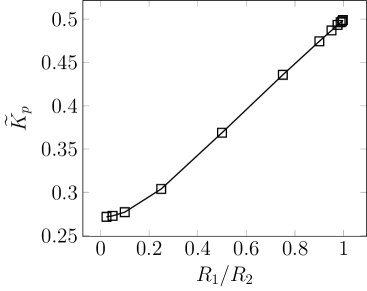
Figure 2. Numerical investigation of the Poincaré inequality on annular domains (Example 6.1). Left: Linear scaling of the (approximate) smallest eigenvalue of (6.6) related to the constant $K_{p}\epsilon$ in (6.5). Right: Dependence of $K_{p}$ on the ratio of radii reveals that both limits $R_{1}\rightarrow 0$ and $R_{1}\rightarrow R_{2}$ lead to bounded $K_{p}$.

For a convex and regular domain such as a circle or ellipse, it is well-known that a Sobolev trace inequality holds [6]. However, is this also the case for (nearly) annular domains? The subsequent Lemma 6.2 addresses this question affirmatively.

Lemma 6.2 (Trace inequality over $\Theta$).

For a.e. $s\in\Lambda$ and $t\in(0,T]$, the following trace inequality holds with $K_{\mathrm{tr}}$ independent of $\epsilon(s,t)$:

(6.7) $$\|v\|_{L^{2}(\partial\Theta(s,t))}^{2}\leq K_{\mathrm{tr}}\left(\epsilon(s,t)^{-1}\|v\|_{L^{2}(\Theta(s,t))}^{2}+\epsilon(s,t)\|\nabla v\|_{L^{2}(\Theta(s,t))}^{2}\right)\quad v\in H^{1}(\Theta(s,t)),$$

where $\epsilon(s,t)=\mathrm{diam}(\Theta(s,t))$.

Proof.

For the circular case, if $\Theta(s)=\{(r\cos(\theta),r\sin(\theta)),0\leq r<R_{2}(s,\theta),0\leq\theta\leq 2\pi\}$, this inequality is well known, Section 1.6 in [6]. We use similar arguments to extend the proof to an annulus.

Suppose now that $R_{1}>0$ and let $\Theta(s)=\{(r\cos(\theta),r\sin(\theta)),R_{1}(s,\theta)<r<R_{2}(s,\theta),0\leq\theta\leq 2\pi\}$. We omit $s,t$ in the notation for the sake of brevity. Let $(r,\theta)\in(R_{1},R_{2})\times[0,2\pi]$. We write

$$R_{1}^{2}u^{2}(R_{1},\theta)-r^{2}u^{2}(r,\theta)=-\int_{R_{1}}^{r}\partial_{z}(z^{2}u^{2}(z,\theta))\,\mathrm{d}z.$$

Here, for simplicity, we write $u(r,\theta)=u(r\cos(\theta),r\sin(\theta))$. Thus, we have that

$$R_{1}^{2}u^{2}(R_{1},\theta)\leq r^{2}u^{2}(r,\theta)+\int_{R_{1}}^{r}|\partial_{z}(z^{2}u^{2}(z,\theta))|\,\mathrm{d}z.$$

Integrating over $(R_{1},R_{2})$ and over $[0,2\pi]$, we find that

$$R_{1}(R_{2}-R_{1})\|u\|^{2}_{L^{2}(\partial\Theta_{1})}\leq R_{2}\|u\|^{2}_{L^{2}(\Theta)}\\ +\int_{0}^{2\pi}\int_{R_{1}}^{R_{2}}\int_{R_{1}}^{r}2|u(z,\theta)|\,|\partial_{z}u(z,\theta)|z^{2}\,\mathrm{d}z\,\mathrm{d}r\,\mathrm{d}\theta+\int_{0}^{2\pi}\int_{R_{1}}^{R_{2}}\int_{R_{1}}^{r}2zu^{2}(z,\theta)\,\mathrm{d}z\,\mathrm{d}r\,\mathrm{d}\theta,$$

where $\partial\Theta_{1}$ denotes the inner circle of $\Theta$. Simplifying the last term and using Cauchy–Schwarz inequality for the penultimate, we obtain:

$$R_{1}(R_{2}-R_{1})\|u\|^{2}_{L^{2}(\partial\Theta_{1})}\leq(R_{2}+2(R_{2}-R_{1}))\|u\|^{2}_{L^{2}(\Theta)}+2(R_{2}-R_{1})R_{2}\|u\|_{L^{2}(\Theta)}\|\nabla u\|_{L^{2}(\Theta)}.$$

With assumption (6.3) and Young’s inequality, we obtain:

$$\|u\|^{2}_{L^{2}(\partial\Theta_{1})}\lesssim\epsilon^{-1}\|u\|^{2}_{L^{2}(\Theta)}+\epsilon\|\nabla u\|^{2}_{L^{2}(\Theta)}.$$

Similar arguments yield the same bound over the outer circle $\partial\Theta_{2}$ for $\|u\|_{L^{2}(\partial\Theta_{2})}^{2}$. Adding the two bounds gives the result. The above computations are for smooth functions. The result for functions in $H^{1}(\Theta)$ follows by density. ∎

We now turn to consider a trace inequality for the surrounding domain $\Omega_{s}$ (Lemma 6.4) by way of an extension operator (Lemma 6.3) first introduced and studied in [53].

Lemma 6.3 (Extension operator).

For any $t\in[0,T]$ and $k\in\{1,2\}$, there exists an extension operator $\mathcal{E}(t):H^{k}(\Omega_{s}(t))\rightarrow H^{k}(\Omega)$ satisfying $\mathcal{E}(t)v|_{\Omega_{s}(t)}=v|_{\Omega_{s}(t)},\,\,\mathcal{E}(t)v|_{\Gamma(t)}=v|_{\Gamma(t)}$ and such that

(6.8) $$\|\mathcal{E}(t)v\|_{H^{k}(\Omega)}\leq K_{\mathcal{E}}\|v\|_{H^{k}(\Omega_{s}(t))},\quad\,\forall v\in H^{k}(\Omega_{s}(t)),$$

with a constant $K_{\mathcal{E}}$ independent of $\epsilon_{\max}$ and $t$.

Proof.

The construction of the extension operator and the proof of the continuity bound are very similar to [53, Theorem 2.1]. For completeness, we provide some details adapted to our geometrical setting. First, we define the extension from a fixed domain $\tilde{B}=B_{1}\backslash B$ to $B_{1}$ where $B$ and $B_{1}$ are cylindrical domains of radii $1$ and $2$ respectively. Let $\mathcal{E}_{0}:H^{1}(\tilde{B})\rightarrow H^{1}(\mathbb{R}^{3})$ be the extension operator as defined in [18, Section 5.4]. We have the following two bounds:

$$\|\mathcal{E}_{0}u\|_{H^{1}(\mathbb{R}^{d})}\leq K_{1}\|u\|_{H^{1}(\tilde{B})},\,\,\,\,\|\mathcal{E}_{0}u\|_{H^{2}(\mathbb{R}^{d})}\leq K_{2}\|u\|_{H^{2}(\tilde{B})}.$$

Let $H^{k}_{0}(B)=\{v\in H^{k}(B),\partial^{\alpha}v=0,\,\,|\alpha|<k\,\,\mathrm{on}\,\,\partial B\}$ and define $z\in H^{k}_{0}(B)$ such that

(6.9) $$\sum_{|\alpha|=k}(\partial^{\alpha}z,\partial^{\alpha}q)_{B}=\sum_{|\alpha|=k}(\partial^{\alpha}(\mathcal{E}_{0}u),\partial^{\alpha}q)_{B},\,\,\,\forall q\in H^{k}_{0}(B).$$

One can show that $z$ is well-defined by the Lax-Milgram theorem since a Poincaré inequality holds in $H^{k}_{0}(B)$, and we have that

(6.10) $$\|z\|_{H^{k}(B)}\leq\tilde{K}_{k}\|\mathcal{E}_{0}u\|_{H^{k}(B)}.$$

The extension operator $\mathcal{E}_{\tilde{B}}:H^{1}(\tilde{B})\to H^{1}(B_{1})$ is then defined as follows:

(6.11) $$\mathcal{E}_{\tilde{B}}u\,(\boldsymbol{x})=\begin{cases}u(\boldsymbol{x}),&\boldsymbol{x}\in\tilde{B}\\ \mathcal{E}_{0}u(\boldsymbol{x})-z(\boldsymbol{x}),&\boldsymbol{x}\in B\end{cases}.$$

To show continuity of $\mathcal{E}_{\tilde{B}}$, we have that for $k\in\{1,2\}$:

(6.12) $$\|\mathcal{E}_{\tilde{B}}u\|^{2}_{H^{k}(B_{1})}=\|u\|^{2}_{H^{k}(\tilde{B})}+\|\mathcal{E}_{0}u-z\|_{H^{k}(B)}^{2}\leq\|u\|^{2}_{H^{k}(\tilde{B})}+(\|\mathcal{E}_{0}u\|_{H^{k}(B)}+\|z\|_{H^{k}(B)})^{2}\\ \leq\|u\|^{2}_{H^{k}(\tilde{B})}+(1+\tilde{K}_{k})^{2}K^{2}_{k}\|u\|^{2}_{H^{k}(\tilde{B})}\leq K_{k}^{f}\|u\|^{2}_{H^{k}(\tilde{B})}.$$

In the above, we let $K^{f}_{k}=1+(1+\tilde{K}_{k})^{2}K^{2}_{k}$ which clearly depends on $B,\tilde{B}$ and $B_{1}$. A key property of this extension is that $\mathcal{E}_{\tilde{B}}p=p$ for all polynomials $p$ of degree less than $k$, see [53, Lemma 2.1]. By choosing $p$ as the average of $u$ for $k=1$ or the Lagrange interpolant of degree $1$ for $k=2$, this observation yields the following bounds on the semi-norms:

(6.13) $$|\mathcal{E}_{\tilde{B}}u|^{2}_{H^{k}(B_{1})}=|\mathcal{E}_{\tilde{B}}(u-p)|^{2}_{H^{k}(B_{1})}\leq K_{k}^{f}\|u-p\|^{2}_{H^{k}(\tilde{B})}\leq K_{k}^{f}K_{2}|u|^{2}_{H^{k}(\tilde{B})},$$

for some constant $K_{2}$. Now, we define the extension operator from $H^{k}(\Omega_{s}(t))\to H^{k}(\Omega)$ as:

(6.14) $$\mathcal{E}(t)v=\begin{cases}\mathcal{E}_{\tilde{B}}(v\circ\chi_{R_{2}(t)}^{-1})\circ\chi_{R_{2}(t)},&\mathrm{in}\,\,B_{2\,R_{2}(t)}\\ v,&\mathrm{in}\,\,\Omega_{s}(t)\backslash B_{2\,R_{2}(t)}\end{cases},$$

where $B_{2R_{2}(t)}$ is the cylinder surrounding $B_{R_{2}}$ of radius $2R_{2}$ and

$$\chi_{R_{2}(t)}((s,R_{2}\cos(\theta),R_{2}\sin(\theta)))=(s,\cos(\theta),\sin(\theta)),\,\,\,\forall(s,\theta)\in\Lambda\times[0,2\pi].$$

The continuity of $\mathcal{E}$ then follows from a scaling argument and (6.3) which yield that

$$|v\circ\chi_{R_{2}(t)}^{-1}|^{2}_{H^{i}(\tilde{B})}\lesssim\epsilon_{\max}^{-3+2i}|v|^{2}_{H^{i}(B_{2R_{2}(t)}\backslash B_{R_{2}(t)})},\,\,\,|\hat{v}\circ\chi_{R_{2}(t)}|^{2}_{H^{i}(B_{2R_{2}(t)})}\lesssim\epsilon_{\max}^{3-2i}|\hat{v}|^{2}_{H^{i}(B_{1})},$$

for $i\in\{0,1,2\}.$ Thus, we obtain the following:

(6.15) $$\begin{split}\|\mathcal{E}(t)v\|_{H^{k}(\Omega)}^{2}&=\|v\|_{H^{k}(\Omega_{s}(t)\backslash B_{2\,R_{2}(t)})}^{2}+\|\mathcal{E}_{\tilde{B}}(v\circ\chi_{R_{2}(t)}^{-1})\circ\chi_{R_{2}(t)}\|_{H^{k}(B_{2\,R_{2}(t)})}^{2}\\ &\lesssim\|v\|_{H^{k}(\Omega_{s}(t))}^{2}+\sum_{i=0}^{k}\epsilon_{\max}^{3-2i}|\mathcal{E}_{\tilde{B}}(v\circ\chi_{R_{2}(t)}^{-1})|^{2}_{H^{i}(B_{1})}\\ &\leq\|v\|_{H^{k}(\Omega_{s}(t))}^{2}+\sum_{i=0}^{k}\epsilon_{\max}^{3-2i}K_{k}^{f}K_{2}|v\circ\chi_{R_{2}(t)}^{-1}|^{2}_{H^{i}(\tilde{B})}\\ &\lesssim\|v\|^{2}_{H^{k}(\Omega_{s}(t))}.\qed\end{split}$$

Lemma 6.4 (Trace inequality over $\Omega_{s}$).

There exists a constant $K_{\Gamma}$ independent of $t$ and of $\epsilon_{\max}$ such that

(6.16) $$\|v\|_{L^{2}(\Gamma(t))}\leq K_{\Gamma}(\epsilon_{\max}\,|\ln\epsilon_{\max}|)^{1/2}\,\|v\|_{H^{1}(\Omega_{s}(t))},\quad\,\forall v\in H^{1}(\Omega_{s}(t)).$$

Proof.

Without loss of generality, we consider the case of $\Omega_{v}$ being an annular cylinder domain and $\Omega_{s}$ its outer surroundings. We have for $v\in H^{1}(\Omega_{s}(t))$:

(6.17) $$\|v\|^{2}_{L^{2}(\Gamma(t))}=\|\mathcal{E}v\|_{L^{2}(\Gamma(t))}^{2}=\int_{\Lambda}\|\mathcal{E}v\|_{L^{2}(\partial\Theta_{2}(s,t))}^{2}\,\mathrm{d}s.$$

We use ideas from the proofs of [34, Lemma 2.1 and Lemma 2.2] where we adapt the arguments to 3D. We write for a.e. $s\in\Lambda,t\geq 0$,

(6.18) $$\|\mathcal{E}v\|_{L^{2}(\partial\Theta_{2}(s,t))}\leq\|\mathcal{E}v-\overline{\mathcal{E}v}\|_{L^{2}(\partial\Theta_{2}(s,t))}+\|\overline{\mathcal{E}v}\|_{L^{2}(\partial\Theta_{2}(s,t))}.$$

The first term is bounded by a Stekloff type inequality [38]:

(6.19) $$\|\mathcal{E}v-\overline{\mathcal{E}v}\|_{L^{2}(\partial\Theta_{2}(s,t))}\leq K_{\mathrm{st}}\epsilon(s,t)^{1/2}\|\nabla(\mathcal{E}v)\|_{L^{2}(\Theta_{2}(s,t))}.$$

For the second term in (6.18), observe that by definition of the perimeter average

(6.20) $$\|\overline{\mathcal{E}v}\|_{L^{2}(\partial\Theta_{2}(s,t))}=|\partial\Theta_{2}(s,t)|^{1/2}|\overline{\mathcal{E}v}|.$$

From the proof of [34, Lemma 2.1], we further have for $p>2$

(6.21) $$|\overline{\mathcal{E}v}|\leq\left(\pi R_{2}(s,t)^{2}\right)^{-1/p}\|\mathcal{E}v\|_{L^{p}(\Theta_{2}(s,t))}+\frac{1}{2\sqrt{\pi}}\|\nabla\mathcal{E}{v}\|_{L^{2}(\Theta_{2}(s,t))}.$$

Hence, we obtain:

(6.22) $$\|\overline{\mathcal{E}v}\|_{L^{2}(\partial\Theta_{2}(s,t))}\leq K\left(\epsilon(s,t)^{1/2-2/p}\|\mathcal{E}v\|_{L^{p}(\Theta_{2}(s,t))}+\epsilon(s,t)^{1/2}\|\nabla\mathcal{E}v\|_{L^{2}(\Theta_{2}(s,t))}\right).$$

Upon substituting in (6.17), we have that

(6.23) $$\int_{\Lambda}\|\mathcal{E}v\|_{L^{2}(\partial\Theta_{2}(s,t))}^{2}\leq K\int_{\Lambda}(\epsilon_{\max}^{1-4/p}\|\mathcal{E}v\|_{L^{p}(\Theta_{2}(s,t))}^{2}+\epsilon_{\max}\|\nabla\mathcal{E}v\|^{2}_{L^{2}(\Theta_{2}(s,t))}).$$

Consider now a fixed cylindrical domain $B_{\Lambda}$ around the centerline $\Lambda$ with cross-sections $\Theta_{\Lambda}(s,t)$. We emphasize that $B_{\Lambda}$ does not depend on $\epsilon_{\max}$. Observe that for $\epsilon_{\max}$ small, $\Omega_{v}(t)\subset B_{\Lambda}$. Let $\tilde{B}_{\Lambda}$ be another cylinder such that $B_{\Lambda}\subset\tilde{B}_{\Lambda}\subset\Omega$ with cross-sections $\tilde{\Theta}_{\Lambda}(s,t)\supset\Theta_{\Lambda}(s,t)$. Define $\chi$ to be a smooth cut-off function on $B_{\Lambda}$ such that $\chi=1$ in $B_{\Lambda}$ with compact support in $\tilde{B}_{\Lambda}$. By construction, we have

$$\|\mathcal{E}v\|_{L^{p}(\Theta_{2}(s,t))}\leq\|\mathcal{E}v\|_{L^{p}(\Theta_{\Lambda}(s,t))}=\|\chi(\mathcal{E}v)\|_{L^{p}(\Theta_{\Lambda}(s,t))}\leq\|\chi(\mathcal{E}v)\|_{L^{p}(\tilde{\Theta}_{\Lambda}(s,t))}.$$

Since $\chi(\mathcal{E}v)\in H^{1}_{0}(\tilde{\Theta}_{\Lambda}(s,t))$, we apply the Sobolev embedding result in 2D which gives a constant with an explicit dependence on $p$ [57, eq (6.20)]:

$$\|\chi(\mathcal{E}v)\|_{L^{p}(\tilde{\Theta}_{\Lambda}(s,t))}\leq Kp^{1/2}\|\nabla(\chi(\mathcal{E}v))\|_{L^{2}(\tilde{\Theta}_{\Lambda}(s,t))}\leq Kp^{1/2}\|\mathcal{E}v\|_{H^{1}(\tilde{\Theta}_{\Lambda}(s,t))}.$$

The above constant depends on $\tilde{\Theta}_{\Lambda}(s,t)$ and on $\chi$ but not $\epsilon_{\max}$. Substituting in (6.23), and choosing $p=|\ln\epsilon_{\max}|$ yields:

$$\|\mathcal{E}v\|_{L^{2}(\Gamma(t))}^{2} \leq K\int_{\Lambda}\left(\epsilon_{\max}|\ln\epsilon_{\max}|\|\mathcal{E}v\|_{H^{1}(\tilde{\Theta}_{\Lambda}(s,t))}^{2}+\epsilon_{\max}\|\nabla\mathcal{E}v\|^{2}_{L^{2}(\Theta_{2}(s,t))}\right)$$

$$\leq K\epsilon_{\max}\left(|\ln\epsilon_{\max}|\|\mathcal{E}v\|_{H^{1}(\tilde{B}_{\Lambda})}^{2}+\|\mathcal{E}v\|_{H^{1}(\Omega)}^{2}\right)\leq K\epsilon_{\max}|\ln\epsilon_{\max}|\|\mathcal{E}v\|_{H^{1}(\Omega)}^{2}.$$

Using (6.8) in the above concludes the proof.

∎

Example 6.2 (Trace inequality over $\Omega_{s}$).

The scaling law of Lemma 6.4 can be demonstrated numerically by considering the following Stekloff eigenvalue problem [55]: find $u\in H^{1}(\Omega_{s})$ and $\lambda>0$ such that

(6.24) $$\Delta u =u \quad\text{ in }\Omega_{s},$$

$$\nabla u\cdot\boldsymbol{n} =\lambda u \quad\text{ on }\Gamma,$$

$$\nabla u\cdot\boldsymbol{n} =0 \quad\text{ on }\partial\Omega_{s}\setminus\Gamma.$$

More precisely, for $\lambda_{1}$ being the smallest non-zero eigenvalue of (6.24), there holds that

(6.25) $$\|u\|_{L^{2}(\Gamma)}\leq\lambda_{1}^{-1/2}\|u\|_{H^{1}(\Omega_{s})},\quad\,\forall v\in H^{1}(\Omega_{s}).$$

Thus, approximations to $\lambda_{1}$ in (6.24) can be used to estimate the bound in (6.16). Now, consider an embedding domain $\Omega_{s}$ (also) in the shape of an cylinder with unit height and unit outer radius. Consider an inner cylinder $\Omega_{v}$ with diameter $\epsilon=2R_{1}$ (and unit height) and consider a decreasing sequence of $R_{1}$s. As in Example 6.1, we approximate this smallest non-zero eigenvalue using the discretization of (6.24) by continuous linear elements defined relative to a series of uniformly refined meshes, and deem the eigenvalues converged when the relative difference between refinements is less then 5%. Clearly, the trace constant decreases with decreasing $\epsilon_{\max}$ (Figure 3). We note that the data are well-fitted by the theoretically established $\epsilon_{\max}^{1/2}\lvert\ln\epsilon_{\max}\rvert^{1/2}$ expression especially for small radii.

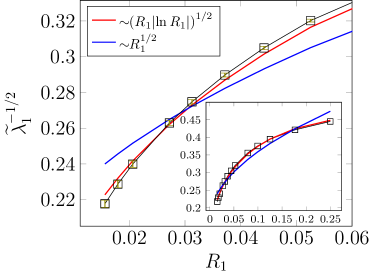
Figure 3. Numerical investigation of the trace inequality (Example 6.2) for vessels of decreasing diameters $\epsilon=2R_{1}$.

7. Analysis of the modelling error

We next turn to address the following question: how large of a modelling error has been introduced by the derivation and associated assumptions of the coupled 3D-1D model in Section 4.3? We begin by considering the modelling error associated with the cross-section average concentration in the vessel, before turning to the modelling error in the surroundings. We will make use of a duality argument, and therefore introduce and analyze the stability of an associated dual problem before turning to the modelling error estimates.

7.1. Well-posedness and stability of a dual transport problem

We consider the properties of a backward-in-time dual transport problem, defined in association with the forward vessel transport problem of 3.1, in Lemma 7.1. A key aspect is to appropriately account for the moving domain and time-derivatives with respect to moving frames. We therefore explicitly track the domain dependence on time $t$.

Lemma 7.1 (Backward-in-time dual problem).

The following problem is well posed: given $g\in L^{2}(0,T;L^{2}(\Omega_{v}(t)))$, find $h\in W=\{L^{2}(0,T;H^{1}(\Omega_{v}(t)))\mid\dot{h}\in L^{2}(0,T;H^{-1}(\Omega_{v}(t)))\}$ and $h(T)=0$ in $\Omega_{v}(T)$ such that for $t\in(0,T)$ and for all $\varphi\in H^{1}(\Omega_{v}(t))$:

(7.1) $$-\langle\dot{h}(t),\varphi\rangle_{H^{-1}(\Omega_{v}(t))}+(D_{v}\nabla h(t),\nabla\varphi)_{\Omega_{v}(t)}+(\xi h(t),\varphi)_{\Gamma(t)}\\ -((\boldsymbol{u}_{v}-\boldsymbol{w})\cdot\nabla h(t),\varphi)_{\Omega_{v}(t)}=(g(t),\varphi)_{\Omega_{v}(t)}.$$

In addition, the following stability bound holds

(7.2) $$\|h\|_{L^{\infty}(0,T;L^{2}(\Omega_{v}(t)))}+\|D_{v}^{1/2}\nabla h\|_{L^{2}(0,T;L^{2}(\Omega_{v}(t)))}\\ +\|\xi^{1/2}h\|_{L^{2}(0,T;L^{2}(\Gamma(t)))}\leq K_{b}\|g\|_{L^{2}(0,T;L^{2}(\Omega_{v}(t)))},$$

where $K_{b}$ is independent of $\epsilon_{\max}$ but depends on the final time $T$, on $\|\nabla\cdot\boldsymbol{w}\|_{L^{\infty}(0,T;L^{\infty}(\Omega))}$, and on $\|D_{v}^{-1/2}\tilde{\boldsymbol{u}}_{v}\|_{L^{\infty}(0,T;L^{\infty}(\Omega_{v}(t)))}$.

Proof.

We consider the forward-in-time solution $z\in W$ and $z(0)=0$ in $\tilde{\Omega}_{v}(0)$ solving for all $\varphi\in H^{1}(\tilde{\Omega}_{v}(t))$

$$\langle\dot{z},\varphi\rangle_{H^{-1}(\tilde{\Omega}_{v}(t))}+(\overset{\leftarrow}{D_{v}}\nabla z,\nabla\varphi)_{\tilde{\Omega}_{v}(t)}+(\overset{\leftarrow}{\xi}z,\varphi)_{\tilde{\Gamma}(t)}-((\overset{\leftarrow}{{\boldsymbol{u}}_{v}}-\overset{\leftarrow}{\boldsymbol{w}})\cdot\nabla z,\varphi)_{\tilde{\Omega}_{v}(t)}=(\overset{\leftarrow}{g},\varphi)_{\tilde{\Omega}_{v}(t)},$$

where a $``\leftarrow"$ over a function indicates that we reverse the time, e.g., $\overset{\leftarrow}{g}(t)=g(T-t)$. The domain $\tilde{\Omega}_{v}(t)=\Omega_{v}(T-t)$ (similarly $\tilde{\Gamma}(t)=\Gamma(T-t)$) is given by the flow map $\overset{\leftarrow}{\boldsymbol{\psi}}(\boldsymbol{x},t)=\boldsymbol{\psi}(\boldsymbol{x},T-t)$. Setting $h(t)=z(T-t)$ for $t\in[0,T]$, we recover the solution to (7.1) since $\dot{h}=-\dot{z}$ and $h(T)=z(0)=0$. Verifying the existence and uniqueness of $z$ then follows from the abstract framework in [3] and from very similar arguments to the proof of Proposition 3.1.

Moreover, choose $\varphi=h\in L^{2}(0,T;H^{1}(\Omega_{v}(t)))$ in (7.1), integrate over time $\tau\in[t,T]$ and use the following formula [3, Theorem 2.40 and Corollary 2.41]:

(7.3) $$-2\int_{t}^{T}\langle\dot{h},h\rangle_{H^{-1}(\Omega_{v}(\tau))}\mathrm{d}\tau=\|h(t)\|^{2}_{L^{2}(\Omega_{v}(t))}+\int_{t}^{T}(h,h\nabla\cdot\boldsymbol{w})_{\Omega_{v}(\tau)}\mathrm{d}\tau.$$

Along with Hölder’s inequality, this yields:

(7.4) $$\frac{1}{2}\|h(t)\|^{2}_{L^{2}(\Omega_{v}(t))}+\|D_{v}^{1/2}\nabla h\|^{2}_{L^{2}(t,T;L^{2}(\Omega_{v}))}+\|\xi^{1/2}h\|^{2}_{L^{2}(t,T;L^{2}(\Gamma))}\\ \leq\|g\|_{L^{2}(t,T;L^{2}(\Omega_{v}(t)))}\|h\|_{L^{2}(t,T;L^{2}(\Omega_{v}(t)))}+\frac{1}{2}\|\nabla\cdot\boldsymbol{w}\|_{L^{\infty}(0,T;L^{\infty}(\Omega_{v}(t)))}\|h\|^{2}_{L^{2}(t,T;L^{2}(\Omega_{v}(t)))}\\ +\|D_{v}^{-1/2}\tilde{\boldsymbol{u}}_{v}\|_{L^{\infty}(0,T;L^{\infty}(\Omega_{v}(t)))}\|h\|_{L^{2}(t,T;L^{2}(\Omega_{v}(t)))}\|D_{v}^{1/2}\nabla h\|_{L^{2}(t,T;L^{2}(\Omega_{v}(t)))}.$$

Applying Young’s inequality for the first and last term on the right hand side above results in:

$$\frac{1}{2}\|h(t)\|^{2}_{L^{2}(\Omega_{v}(t))}+\frac{1}{2}\|D_{v}^{1/2}\nabla h\|^{2}_{L^{2}(t,T;L^{2}(\Omega_{v}))}+\|\xi^{1/2}h\|^{2}_{L^{2}(t,T;L^{2}(\Gamma))}\leq\frac{1}{2}\|g\|^{2}_{L^{2}(0,T;L^{2}(\Omega_{v}(t)))}\\ +\frac{1}{2}\left(1+\frac{1}{2}\|\nabla\cdot\boldsymbol{w}\|_{L^{\infty}(0,T;L^{\infty}(\Omega_{v}(t)))}+\|D_{v}^{-1/2}\tilde{\boldsymbol{u}}_{v}\|^{2}_{L^{\infty}(0,T;L^{\infty}(\Omega_{v}(t)))}\right)\|h\|^{2}_{L^{2}(t,T;L^{2}(\Omega_{v}(t)))}.$$

The result can then be concluded by Grönwall’s inequality, see e.g [18, Appendix B.k]. ∎

7.2. Model error introduced in the derivation of the 1D model

With this dual stability result at hand, we now turn to our first main modelling error estimate, namely comparing (the extension of) the cross-section average vessel solution $\hat{c}:\Lambda\times(0,T)\rightarrow\mathbb{R}$ with its reference solution $c_{v}:\Omega_{v}\times(0,t)\rightarrow\mathbb{R}$, the weak solution of (3.1a). More specifically, we aim to quantify the modelling error

$$\|c_{v}-E\hat{c}\|_{L^{2}(0,T;L^{2}(\Omega_{v}))}.$$

The (constant cross-section) extension $E$ from $H^{1}(\Lambda)$ to $H^{1}(\Omega_{v})$ is given by

(7.5) $$E\hat{c}(s,r,\theta,t)=\hat{c}(s,t),\quad\,\forall(r,\theta)\in\Theta(s,t),\quad\,\forall(s,t)\in\Lambda\times(0,T).$$

We will frequently write $\hat{c}=E\hat{c}$ when context allows this simplification. 7.1 gives the main modelling error estimate for the solutions in the vessel.

Proposition 7.1 (Model error in the vessel).

Let $c_{v},c_{s}$ be weak solutions to the coupled 3D-3D transport problem (3.11) and assume that $c_{v}(0)\in H^{1}(\Omega_{v})$. Let $c,\hat{c}$ be the weak solutions to the reduced coupled 3D-1D problem (4.20) with $w_{c}=1$. Then,

(7.6) $$\|c_{v}-\hat{c}\|_{L^{2}(0,T;L^{2}(\Omega_{v}))}\\ \lesssim K_{b}\,K_{p}\left(\|f_{v}\|_{L^{2}(0,T;H^{1}(\Omega_{v}))}+\|\nabla c_{v}(0)\|_{L^{2}(\Omega_{v})}\right)\epsilon_{\max}+(K_{b}\,K_{\Gamma}\,C_{2})\,\,\epsilon_{\max}^{1/2}|\ln\epsilon_{\max}|^{1/2}\\ +K_{b}(K_{p}+1)(K_{\mathrm{tr}}+1)C_{1}\left(\epsilon_{\max}^{1/2}+\|u_{v,r}\|_{L^{\infty}(0,T;L^{\infty}(\Omega_{v}(t)))}+\|u_{v,\theta}\|_{L^{\infty}(0,T;L^{\infty}(\Omega_{v}(t)))}+\epsilon_{s}\right).$$

Here, $C_{1}$ and $C_{2}$ depend on the material parameters and the solutions $c,\hat{c},$ and $c_{s}$ as

$$C_{1}=\left(\max_{s\in\Lambda,t\in[0,T]}\|u_{v,s}\|_{H^{1}(\Theta)}+\|\boldsymbol{w}\|_{L^{\infty}(\Omega)}\right)\|\hat{c}\|_{L^{2}(0,T;L^{2}(\partial\Omega_{v}(t)))}\\ +\|\hat{c}\|_{L^{2}(0,T;H^{1}(\Omega_{v}(t)))}+\|D_{v}\partial_{s}\hat{c}+\hat{c}\hat{u}\|_{L^{2}(0,T;L^{2}(\Omega_{v}(t)))}+\|\xi(\hat{c}-\overline{c})\|_{L^{2}(0,T;L^{2}(\Gamma(t)))},$$

and

$$C_{2}=\|\xi^{1/2}\|_{L^{\infty}(0,T;L^{\infty}(\Gamma(t)))}\left(\|c_{s}\|_{L^{2}(0,T;H^{1}(\Omega_{s}(t)))}+\|c\|_{L^{2}(0,T;H^{1}(\Omega))}\right).$$

In addition, there exists a constant $K$ depending only on the material parameters and the final time $T$ but not on $\epsilon_{\max}$ such that $C_{1}+C_{2}\lesssim K$. Under the additional assumption that

(7.7) $$\|\overline{c}-\overline{c_{s}}\|_{L^{2}(0,T;L^{2}(\Gamma(t)))}\lesssim\epsilon_{\max}^{1/2},$$

bound (7.6) can be improved by replacing its last term by $K_{b}(K_{\mathrm{st}}K_{\mathcal{E}}+1)C_{2}\,\,\epsilon_{\max}^{1/2}$.

Before presenting the proof, we remark that this proposition and in particular (7.6) provides a rigorous bound on the error in the vessel introduced by the derivation of the 3D-1D model. For the error to converge to $0$ as $\epsilon_{\max}\rightarrow 0$, one needs to assume that $u_{v,r}$ and $u_{v,\theta}$ are negligible at least for small $\epsilon_{\max}$. In addition, if $\epsilon_{s}\lesssim\epsilon_{\max}$ as $\epsilon_{\max}\rightarrow 0$, then one recovers a convergence rate of $1/2$ (up to a log factor) with respect to $\epsilon_{\max}$. The additional assumption (7.7) essentially leads to an estimate for the error induced by Assumptions 4.1 and 4.2 of Section 4.2 alone, without those of Section 4.4; i.e. an estimate for the error between $E\hat{c}$ as given in (4.14) and $c_{v}$ the solution of (3.11). In this case, we can remove the log factor.

Proof.

(Proposition 7.1) We proceed in three main steps to (I) derive a first identity for the modelling error by using a duality argument, (II) manipulate this identity by deriving the weak form satisfied by the extended solution $E\hat{c}$, and (III) bound its terms via Poincaré, trace, Stekloff inequalities, and the regularity bound derived in Lemma 7.1.

Step I. We first recall from (3.11) that the reference solution $c_{v}$ satisfies

(7.8) $$\langle\dot{c}_{v},\phi\rangle_{H^{-1}(\Omega_{v}(t))}+(\nabla\cdot\boldsymbol{w}c_{v},\phi)_{\Omega_{v}(t)}+a_{\mathrm{ref}}(c_{v},\phi)=\ell_{\mathrm{ref}}(\phi),\quad\,\forall\phi\in H^{1}(\Omega_{v}(t)),$$

where we have introduced the two forms

$$a_{\mathrm{ref}}(c,\phi) =(D_{v}\nabla c,\nabla\phi)_{\Omega_{v}(t)}+(\xi c,\phi)_{\Gamma(t)}-((\boldsymbol{u}_{v}-\boldsymbol{w})c,\nabla\phi)_{\Omega_{v}(t)} \quad\,\forall c,\phi\in H^{1}(\Omega_{v}(t)),$$

$$\ell_{\mathrm{ref}}(\phi) =(\xi c_{s},\phi)_{\Gamma(t)}+(f_{v},\phi)_{\Omega_{v}(t)} \quad\,\forall\phi\in H^{1}(\Omega_{v}(t)).$$

To estimate the error $e\equiv c_{v}-E\hat{c}$, we proceed by duality. Namely, let $h$ be the solution of (7.1) with $g=e\in L^{2}(0,T;L^{2}(\Omega_{v}(t)))$. From [3, Corollary 2.41] and the fact that $h(T)=0$, the following integration by parts formula holds:

$$\int_{0}^{T}-\langle\dot{h},e\rangle_{H^{-1}(\Omega_{v}(t))}=\int_{0}^{T}\langle\dot{e},h\rangle_{H^{-1}(\Omega_{v}(t))}+\int_{0}^{T}(e,h\nabla\cdot\boldsymbol{w})_{\Omega_{v}(t)}+(e(0),h(0))_{\Omega_{v}(0)}.$$

With this identity, (7.1) tested with $e\in L^{2}(0,T;H^{1}(\Omega_{v}(t)))$ and integrated over $(0,T)$ reads:

$$\int_{0}^{T}\langle\dot{e},h\rangle_{H^{-1}(\Omega_{v}(t))}+\int_{0}^{T}(e,h\nabla\cdot\boldsymbol{w})_{\Omega_{v}(t)}+(e(0),h(0))_{\Omega_{v}(0)}+\int_{0}^{T}a_{\mathrm{ref}}(e,h)=\int_{0}^{T}\|e\|_{L^{2}(\Omega_{v}(t))}^{2}.$$

Subtracting the time-integrated (7.8), combined with the observation that indeed $\dot{\hat{c}}\in L^{2}(0,T;L^{2}(\Omega_{v}(t)))$ (where we write $\hat{c}$ in place of $E\hat{c}$ here and in the following), we obtain the following identity for the modelling error $e$:

(7.9) $$\int_{0}^{T}\|e\|_{L^{2}(\Omega_{v}(t))}^{2}=-\int_{0}^{T}(\dot{\hat{c}},h)_{\Omega_{v}(t)}-\int_{0}^{T}(\hat{c},h\nabla\cdot\boldsymbol{w})_{\Omega_{v}(t)}-\int_{0}^{T}a_{\mathrm{ref}}(\hat{c},h)\\ +\int_{0}^{T}\ell_{\mathrm{ref}}(h)+(e(0),h(0))_{\Omega_{v}(0)}.$$

Step II. Next, we aim to derive an alternative expression for this error identity. By definition of the strong material derivative cf. (3.6):

(7.10) $$\int_{0}^{T}(\dot{\hat{c}},h)_{\Omega_{v}(t)}+\int_{0}^{T}(\hat{c},h\nabla\cdot\boldsymbol{w})_{\Omega_{v}(t)}=\int_{0}^{T}(\partial_{t}\hat{c},h)_{\Omega_{v}(t)}+\int_{0}^{T}(\nabla\cdot(\hat{c}\boldsymbol{w}),h)_{\Omega_{v}(t)}.$$

Note that this definition holds for $\hat{c}\in\{v\in L^{2}(0,T;H^{1}(\Omega_{v}(t)))\,|\,\dot{v}\in L^{2}(0,T;L^{2}(\Omega_{v}(t)))\}$ by density of $\mathcal{D}(0,T;H^{1}(\Omega_{v}(t)))$ in such spaces, [3, Lemma 2.38]. Further, integrating by parts gives

$$(\nabla\cdot(\hat{c}\boldsymbol{w}),h)_{\Omega_{v}(t)}=(\hat{c}\boldsymbol{w}\cdot\boldsymbol{n},h)_{\partial\Omega_{v}(t)}-(\hat{c}\boldsymbol{w},\nabla h)_{\Omega_{v}(t)},$$

while the cross-section average definitions combined with the chain rule yield

$$(\partial_{t}\hat{c},h)_{\Omega_{v}(t)}=(\partial_{t}\hat{c},A\langle h\rangle)_{\Lambda}=(\partial_{t}(A\hat{c}),\langle h\rangle)_{\Lambda}-(\hat{c}\partial_{t}A,\langle h\rangle)_{\Lambda}.$$

We will derive equivalent expressions for the two terms on the right hand side. First for the last term, by definition of the area $A$ and (3.4), we have that:

$$(\hat{c}\partial_{t}A,\langle h\rangle)_{\Lambda}=\int_{\Lambda}\hat{c}\langle h\rangle\partial_{t}\left(\int_{\Theta(t)}1\right)=\int_{\Lambda}\int_{\partial\Theta(t)}\hat{c}\langle h\rangle\boldsymbol{w}\cdot\boldsymbol{n}=(\hat{c}\boldsymbol{w}\cdot\boldsymbol{n},\langle h\rangle)_{\partial\Omega_{v}(t)}.$$

Second, we will address the former term in combination with other terms from (7.9). To this end, denote by $\hat{\boldsymbol{u}}_{v}=(\langle u_{v,s}\rangle,0,0)$. Note by the definition of $a_{\mathrm{ref}}$, the cross-section, and perimeter averages, and by adding and subtracting, that,

(7.11) $$a_{\mathrm{ref}}(\hat{c}, h)-(\hat{c}\boldsymbol{w},\nabla h)_{\Omega_{v}(t)}=(D_{v}\partial_{s}\hat{c},\partial_{s}h)_{\Omega_{v}(t)}+(\xi\hat{c},h)_{\Gamma(t)}-(\boldsymbol{u}_{v}\hat{c},\nabla h)_{\Omega_{v}(t)}$$

$$=(D_{v}A\partial_{s}\hat{c},\langle\partial_{s}h\rangle)_{\Lambda}+(\xi P\hat{c},\overline{h})_{\Lambda}-(\boldsymbol{u}_{v}\hat{c},\nabla{h})_{\Omega_{v}(t)}$$

$$=(D_{v}A\partial_{s}\hat{c},\langle\partial_{s}h\rangle)_{\Lambda}+(\xi P\hat{c},\overline{h})_{\Lambda}-((\boldsymbol{u}_{v}-\hat{\boldsymbol{u}}_{v})\hat{c},\nabla{h})_{\Omega_{v}(t)}-(A\langle u_{v,s}\rangle\hat{c},\langle\partial_{s}h\rangle)_{\Lambda}.$$

We proceed by returning to the weak formulation of the coupled 3D-1D problem (4.20b) with $\hat{v}=\langle h\rangle\in H^{1}_{A}(\Lambda)$. We now invoke the assumption that $w_{c}=1$; then $g_{s}=0$ and $\overline{w_{c}}=1$. Let $\hat{u}=\langle u_{v,s}\rangle$. Then, (4.20b), after combining time-integration terms, gives that

(7.12) $$(\partial_{t}(A\hat{c}),\langle h\rangle)_{\Lambda}+(D_{v}A\partial_{s}\hat{c},\partial_{s}\langle h\rangle)_{\Lambda}-(A\hat{u}\hat{c},\partial_{s}\langle h\rangle)_{\Lambda}+(\xi P(\hat{c}-\bar{c}),\langle h\rangle)_{\Lambda}=(A\langle f_{v}\rangle,\langle h\rangle)_{\Lambda}.$$

Observe that

(7.13) $$A\partial_{s}\langle h\rangle=\partial_{s}(A\langle h\rangle)-\langle h\rangle\partial_{s}A=A\langle\partial_{s}h\rangle+\int_{\partial\Theta_{2}}(h-\langle h\rangle)\partial_{s}R_{2}-\int_{\partial\Theta_{1}}(h-\langle h\rangle)\partial_{s}R_{1}.$$

Using (7.13) and (7.11) in (7.12), we obtain:

(7.14) $$(\partial_{t}(A\hat{c}),\langle h\rangle)_{\Lambda}+a_{\mathrm{ref}}(\hat{c},h)-(\hat{c}\boldsymbol{w},\nabla h)_{\Omega_{v}(t)}=-((\boldsymbol{u}_{v}-\hat{\boldsymbol{u}}_{v})\hat{c},\nabla{h})_{\Omega_{v}(t)}+\ell(h)-\ell_{1}(h),$$

where we have introduced the short-hand

$$\ell(h) =\int_{\Lambda}\xi P\overline{c}\,\overline{h}+\int_{\Lambda}A\langle f_{v}\rangle\langle h\rangle=(\xi\overline{c},h)_{\Gamma}+(\langle f_{v}\rangle,h)_{\Omega_{v}},$$

$$\ell_{1}(h) =\int_{\Lambda}(-D_{v}\partial_{s}\hat{c}+\hat{c}\hat{u})\left(\int_{\partial\Theta_{1}}(h-\langle h\rangle)\partial_{s}R_{1}-\int_{\partial\Theta_{2}}(h-\langle h\rangle)\partial_{s}R_{2}\right)-(\xi(\langle h\rangle-\bar{h}),\overline{c}-\hat{c})_{\Gamma(t)}.$$

Collecting all the above expressions in (7.9) yields:

(7.15) $$\int_{0}^{T}\|e\|_{L^{2}(\Omega_{v}(t))}^{2}=\int_{0}^{T}((\boldsymbol{u}_{v}-\hat{\boldsymbol{u}}_{v})\hat{c},\nabla h)_{\Omega_{v}(t)}-\int_{0}^{T}(\hat{c}\boldsymbol{w}\cdot\boldsymbol{n},h-\langle h\rangle)_{\partial\Omega_{v}(t)}\\ +\int_{0}^{T}\left(\ell_{\mathrm{ref}}(h)-\ell(h)\right)+\int_{0}^{T}\ell_{1}(h)+(e(0),h(0))_{\Omega_{v}(0)}:=\sum_{i=1}^{5}W_{i}.$$

Step III. We now bound each term $W_{i}$ ($i=1,\dots,5$) on the right-hand side of (7.15). For brevity, we omit the time-dependence of the domains in the notation in the below. For $W_{1}$, write

$$W_{1}=\int_{0}^{T}((0,u_{v,r},u_{v,\theta})\hat{c},\nabla h)_{\Omega_{v}}+\int_{0}^{T}(u_{v,s}-\langle u_{v,s}\rangle)\hat{c}\partial_{s}h=W_{1,1}+W_{1,2}.$$

An application of Hölder’s inequality yields

$$W_{1,1}\equiv\int_{0}^{T}((0,u_{v,r},u_{v,\theta})\hat{c},\nabla h)_{\Omega_{v}}\leq\int_{0}^{T}(\|u_{v,r}\|_{L^{\infty}(\Omega_{v})}+\|u_{v,\theta}\|_{L^{\infty}(\Omega_{v})})\|\hat{c}\|_{L^{2}(\Omega_{v})}\|h\|_{H^{1}(\Omega_{v})}.$$

For $W_{1,2}$, with Hölder’s and Poincaré’s inequality (6.5), we have that

$$W_{1,2} =\int_{0}^{T}\int_{\Lambda}\hat{c}\int_{\Theta}(u_{v,s}-\langle u_{v,s}\rangle)\partial_{s}h\leq\int_{0}^{T}\int_{\Lambda}|\hat{c}|\|u_{v,s}-\langle u_{v,s}\rangle\|_{L^{2}(\Theta)}\|\partial_{s}h\|_{L^{2}(\Theta)}$$

$$\leq K_{p}\int_{0}^{T}\int_{\Lambda}|\hat{c}|\epsilon(s,t)\|\nabla u_{v,s}\|_{L^{2}(\Theta)}\|\partial_{s}h\|_{L^{2}(\Theta)}$$

$$=K_{p}\int_{0}^{T}\int_{\Lambda}\epsilon(s,t)P^{-1/2}\|\hat{c}\|_{L^{2}(\partial\Theta_{2})}\|\nabla u_{v,s}\|_{L^{2}(\Theta)}\|\partial_{s}h\|_{L^{2}(\Theta)}.$$

Thus, with Hölder’s inequality and the assumption that the vessel area and outer perimeter are both bounded in terms of $\epsilon$ but with (implicit) inequality constants independent of $\Omega_{v},\Omega_{s}$ (6.4),

(7.16) $$W_{1,2}\,\lesssim\,K_{p}\int_{0}^{T}\epsilon_{\max}^{1/2}\left(\max_{s\in\Lambda}\|\nabla u_{v,s}\|_{L^{2}(\Theta)}\right)\|\hat{c}\|_{L^{2}(\Gamma)}\|h\|_{H^{1}(\Omega_{v})}.$$

Hence, with Hölder’s inequality again, we obtain the following for $W_{1}$:

(7.17) $$W_{1}=W_{1,1}+W_{1,2}\,\lesssim\,K_{p}\,\,\epsilon_{\max}^{1/2}\max_{s\in\Lambda,t\in[0,T]}\|u_{v,s}\|_{H^{1}(\Theta)}\|\hat{c}\|_{L^{2}(0,T;L^{2}(\Gamma))}\|h\|_{L^{2}(0,T;H^{1}(\Omega_{v}))}\\ +(\|u_{v,r}\|_{L^{\infty}(0,T;L^{\infty}(\Omega_{v}))}+\|u_{v,\theta}\|_{L^{\infty}(0,T;L^{\infty}(\Omega_{v}))})\|\hat{c}\|_{L^{2}(0,T;L^{2}(\Omega_{v}))}\|h\|_{L^{2}(0,T;H^{1}(\Omega_{v}))}.$$

Continuing, we bound $W_{2}$ and $W_{4}$ by first obtaining a bound on $\|\overline{v}-\langle v\rangle\|_{L^{2}(\Gamma)}$ for any $v\in H^{1}(\Omega_{v})$. First note that

$$\|\langle v\rangle-\overline{v}\|_{L^{2}(\partial\Theta)}^{2}=\int_{\partial\Theta}(\langle v\rangle-\overline{v})(\langle v\rangle-\overline{v})=\int_{\partial\Theta}(\langle v\rangle-v)(\langle v\rangle-\overline{v})+\int_{\partial\Theta}(v-\overline{v})(\langle v\rangle-\overline{v})\\ =\int_{\partial\Theta}(\langle v\rangle-v)(\langle v\rangle-\overline{v})\leq\|\langle v\rangle-v\|_{L^{2}(\partial\Theta)}\|\langle v\rangle-\overline{v}\|_{L^{2}(\partial\Theta)}.$$

Using this observation, the trace inequality (6.7), and Poincare’s inequality (6.5), we have that for any $v\in H^{1}(\Theta)$

(7.18) $$\|\langle v\rangle-\bar{v}\|_{L^{2}(\partial\Theta)}\leq\|\langle v\rangle-v\|_{L^{2}(\partial\Theta)}\\ \leq K_{\mathrm{tr}}\left(\epsilon(s,t)^{-1/2}\|\langle v\rangle-v\|_{L^{2}(\Theta)}+\epsilon(s,t)^{1/2}\|\nabla v\|_{L^{2}(\Theta)}\right)\leq K_{\mathrm{tr}}(K_{p}+1)\epsilon_{\max}^{1/2}\|\nabla v\|_{L^{2}(\Theta)}.$$

With Cauchy–Schwarz inequality, we have that:

$$\begin{split}&W_{2}+W_{4}=\int_{0}^{T}(\hat{c}\boldsymbol{w}\cdot\boldsymbol{n},h-\langle h\rangle)_{\partial\Omega_{v}}+\int_{0}^{T}\ell_{1}(h)\\ &\leq\int_{0}^{T}(\|\boldsymbol{w}\|_{L^{\infty}(\Omega)}\|\hat{c}\|_{L^{2}(\partial\Omega_{v})}+\epsilon_{s}\|D_{v}\partial_{s}\hat{c}+\hat{c}\hat{u}\|_{L^{2}(\partial\Omega_{v})}+\|\xi(\hat{c}-\overline{c})\|_{L^{2}(\Gamma)})\|\langle h\rangle-h\|_{L^{2}(\partial\Omega_{v})}\\ &\leq K_{\mathrm{tr}}(K_{p}+1)\epsilon_{\max}^{1/2}\int_{0}^{T}(\|\boldsymbol{w}\|_{L^{\infty}(\Omega)}\|\hat{c}\|_{L^{2}(\partial\Omega_{v})}+\epsilon_{s}\|D_{v}\partial_{s}\hat{c}+\hat{c}\hat{u}\|_{L^{2}(\partial\Omega_{v})}+\|\xi(\hat{c}-\overline{c})\|_{L^{2}(\Gamma)})\|h\|_{H^{1}(\Omega_{v})}\\ &\lesssim K_{\mathrm{tr}}(K_{p}+1)(\epsilon_{\max}^{1/2}\|\boldsymbol{w}\|_{L^{\infty}(0,T;L^{\infty}(\Omega))}\|\hat{c}\|_{L^{2}(0,T;L^{2}(\partial\Omega_{v}))}+\epsilon_{s}\|D_{v}\partial_{s}\hat{c}+\hat{c}\hat{u}\|_{L^{2}(0,T;L^{2}(\Omega_{v}))}\\ &\quad+\epsilon_{\max}^{1/2}\|\xi(\hat{c}-\overline{c})\|_{L^{2}(0,T;L^{2}(\Gamma))})\|h\|_{L^{2}(0,T;H^{1}(\Omega_{v}))}.\end{split}$$

In the above, we used that $\epsilon_{\max}^{1/2}\|D_{v}\partial_{s}\hat{c}+\hat{c}\hat{u}\|_{L^{2}(\partial\Omega_{v})}\lesssim\|D_{v}\partial_{s}\hat{c}+\hat{c}\hat{u}\|_{L^{2}(\Omega_{v})}.$ This follows from the observation that $D_{v},\hat{c},$ and $\hat{u}$ are uniform on each cross-section and from (6.3).

Consider now the definition of $W_{3}$ in combination with Cauchy-Schwarz:

(7.19) $$\begin{split}W_{3}&=\int_{0}^{T}(\xi(c_{s}-\bar{c}),h)_{\Gamma}+(f_{v}-\langle f_{v}\rangle,h)_{\Omega_{v}}\\ &\leq\int_{0}^{T}\|\xi^{1/2}(c_{s}-\overline{c})\|_{L^{2}(\Gamma)}\|\xi^{1/2}h\|_{L^{2}(\Gamma)}+\|f_{v}-\langle f_{v}\rangle\|_{L^{2}(\Omega_{v})}\|h\|_{L^{2}(\Omega_{v})}.\end{split}$$

For the first integrand term of the previous line, we may use the observation that $\|\overline{c}\|_{L^{2}(\Gamma)}=\|\overline{c}\|_{L^{2}_{P}(\Lambda)}\leq\|c\|_{L^{2}(\Gamma)}$ and the trace Lemma 6.4 over $\Omega_{s}$.

$$\|\xi^{1/2}(c_{s}-\overline{c})\|_{L^{2}(\Gamma)}\leq K_{\Gamma}(\epsilon_{\max}|\ln\epsilon_{\max}|)^{1/2}\|\xi\|^{1/2}_{L^{\infty}(\Gamma)}(\|c_{s}\|_{H^{1}(\Omega_{s})}+\|c\|_{H^{1}(\Omega_{s})}).$$

For the last integrand in (7.19), we use the Poincaré inequality (6.5). Combining with Hölder’s inequality, we obtain

$$W_{3}\leq K_{\Gamma}(\epsilon_{\max}|\ln\epsilon_{\max}|)^{1/2}\|\xi\|^{1/2}_{L^{\infty}(\Gamma)}\left(\|c_{s}\|_{L^{2}(0,T;H^{1}(\Omega_{s}))}+\|c\|_{L^{2}(0,T;H^{1}(\Omega))}\right)\|\xi^{1/2}h\|_{L^{2}(0,T;L^{2}(\Gamma))}\\ +K_{p}\epsilon_{\max}\|f_{v}\|_{L^{2}(0,T;H^{1}(\Omega_{v}))}\|h\|_{L^{2}(0,T;L^{2}(\Omega_{v}))}.$$

Alternatively, if the sharper bound (7.7) holds, we then first use the triangle inequality for bounding the first term in (7.19):

$$\|\xi^{1/2}(c_{s}-\overline{c})\|_{L^{2}(\Gamma)}\leq\|\xi^{1/2}(c_{s}-\overline{c_{s}})\|_{L^{2}(\Gamma)}+\|\xi^{1/2}(\overline{c_{s}}-\overline{c})\|_{L^{2}(\Gamma)},$$

and then a Stekloff-type inequality along with the boundedness of the extension operator $\mathcal{E}$ (6.8), giving:

$$\|c_{s}-\overline{c_{s}}\|^{2}_{L^{2}(\Gamma)}=\int_{\Lambda}\|\mathcal{E}c_{s}-\overline{\mathcal{E}c_{s}}\|^{2}_{L^{2}(\partial\Theta_{2})}\leq K_{\mathrm{st}}\epsilon_{\max}\int_{\Lambda}\|\nabla\mathcal{E}c_{s}\|^{2}_{L^{2}(\Theta_{2})}\leq K_{\mathrm{st}}K_{\mathcal{E}}\epsilon_{\max}\|c_{s}\|^{2}_{H^{1}(\Omega_{s})}.$$

Then $W_{3}$ can instead be bounded by:

$$W_{3}\lesssim(K_{\mathrm{st}}K_{\mathcal{E}}+1)\epsilon_{\max}^{1/2}\|c_{s}\|_{L^{2}(0,T;H^{1}(\Omega_{s}))}\|\xi h\|_{L^{2}(0,T;L^{2}(\Gamma))}\\ +K_{p}\epsilon_{\max}\|f_{v}\|_{L^{2}(0,T;H^{1}(\Omega_{v}(t)))}\|h\|_{L^{2}(0,T;L^{2}(\Omega_{v}(t)))}.$$

The term $W_{5}$ involving the modelling error associated with the initial condition is handled by the Poincaré inequality (6.5),and that $\hat{c}(0)=\langle c_{v}(0)\rangle$:

$$\|(c_{v}-\hat{c})(0)\|^{2}_{L^{2}(\Omega_{v}(0))}=\int_{\Lambda}\int_{\Theta}(c_{v}(0)-\hat{c}(0))^{2}\leq K_{p}\epsilon_{\max}^{2}\int_{\Lambda}\|\nabla c_{v}(0)\|_{L^{2}(\Theta)}^{2}\\ =K_{p}\epsilon_{\max}^{2}\|\nabla c_{v}(0)\|^{2}_{L^{2}(\Omega_{v}(0))}.$$

This implies that

(7.20) $$W_{5}\leq K_{p}\epsilon_{\max}\|\nabla c_{v}(0)\|^{2}_{L^{2}(\Omega_{v}(0))}\|h(0)\|_{L^{2}(\Omega_{v}(0))}.$$

Collecting all the above bounds in (7.15) and using (7.2) yields the estimate. The proof of the boundedness of $C_{1}$ and $C_{2}$ by a constant $K$ independent of $\epsilon_{\max}$ is given in the Appendix, section A.1. ∎

7.3. Model error introduced in the surrounding 3D domain

In this subsection, we study the error introduced in the model derivation of the extended transport model (Section 4.4). In particular, we aim to study the difference $(c_{s}-c)$ between the reference solution $c_{s}\in L^{2}(0,T;H_{\partial\Omega}^{1}(\Omega_{s}(t)))$ satisfying the weak solute transport equations defined over $\Omega_{s}(t)$ (3.11) and the reduced (or perhaps more aptly, extended) solution $c\in L^{2}(0,T;H_{0}^{1}(\Omega))$ satisfying the weak solute transport equations defined over $\Omega$ (4.17). Here, we will assume that $\mathcal{E}D_{s}\in L^{\infty}(0,T;L^{\infty}(\Omega,\mathbb{R}^{3\times 3}))$ with a uniform ellipticity constant $\tilde{\nu}>0$.

We start by recalling the relevant equations and that $\tilde{\boldsymbol{u}}_{s}=\boldsymbol{u}_{s}-\boldsymbol{w}$, we have that $c_{s}$ and $c$ satisfy

(7.21) $$\langle\dot{c}_{s},\phi\rangle_{H^{-1}(\Omega_{s}(t))}+\int_{\Omega_{s}(t)}(\nabla\cdot\boldsymbol{w}c_{s}\phi+D_{s}\nabla c_{s}\cdot\nabla\phi-(\tilde{\boldsymbol{u}}_{s}c_{s})\cdot\nabla\phi)\\ +\int_{\Gamma(t)}\xi(c_{s}-c_{v})\phi=\int_{\Omega_{s}(t)}f_{s}\phi\quad\,\forall\phi\in H^{1}_{\partial\Omega}(\Omega_{s}(t)),$$

and

(7.22) $$\int_{\Omega}\partial_{t}c\phi+\int_{\Omega}(\mathcal{E}D_{s}\nabla c\cdot\nabla\phi-(\mathcal{E}\boldsymbol{u}_{s}c)\cdot\nabla\phi)+\int_{\Gamma(t)}\xi(\overline{c}-\hat{c})\phi=\int_{\Omega}\mathcal{E}f_{s}\phi\quad\,\forall\phi\in H_{0}^{1}(\Omega).$$

In (7.22), the Eulerian derivative is used since now $\partial\Omega$ is independent of $t$. In (7.22), we used that

(7.23) $$\int_{\Lambda}\xi P(\overline{c}-\hat{c})\overline{\phi}=\int_{\Gamma(t)}\xi(\overline{c}-\hat{c})\phi.$$

As a step on the way towards quantifying $c_{s}-c$ over the whole domain, we introduce an intermediate solution $c_{r}$ solving (7.22) but without the coupling terms and aim to bound $(c_{s}-c_{r})$ and $(c_{r}-c)$. More precisely, let $c_{r}\in L^{2}(0,T;H^{1}_{0}(\Omega))$ with $c_{r}(0)=c(0)=\mathcal{E}c_{s}(0)$ solve

(7.24) $$\int_{\Omega}\partial_{t}c_{r}\phi+\int_{\Omega}\mathcal{E}D_{s}\nabla c_{r}\cdot\nabla\phi-(\mathcal{E}\boldsymbol{u}_{s}c_{r})\cdot\nabla\phi=\int_{\Omega}\mathcal{E}f_{s}\phi$$

for all $t>0$ and for all $\phi\in H^{1}_{0}(\Omega)$. From standard parabolic regularity results, see e.g [18, Chapter 7], and from the continuity of the extension operator (6.8), we have for a convex domain $\Omega$ that:

(7.25) $$\|\partial_{t}c_{r}\|_{L^{2}(0,T;L^{2}(\Omega))}+\|c_{r}\|_{L^{2}(0,T;H^{2}(\Omega))}\leq K(\|\mathcal{E}f_{s}\|_{L^{2}(0,T;L^{2}(\Omega))}+\|c_{r}(0)\|_{H^{1}(\Omega)})\\ \leq K_{r}(\|f_{s}\|_{L^{2}(0,T;H^{1}(\Omega_{s}(t)))}+\|c_{s}(0)\|_{H^{1}(\Omega_{s}(0))}).$$

Here $K_{r}$ depends on $\mathcal{E}D_{s}$, $\mathcal{E}\boldsymbol{u}_{s}$, and the final time $T$.

We proceed by first bounding $c-c_{r}$ in Lemma 7.2, and then consider $c_{r}-c_{s}$ and $c-c_{s}$ in 7.2.

Lemma 7.2 (Estimating $c-c_{r}$).

For $c$ and $c_{r}$ defined by (7.22) and (7.24) respectively, there holds that

(7.26) $$\|c-c_{r}\|_{L^{\infty}(0,T;L^{2}(\Omega))}\leq K_{e_{1}}\epsilon_{\max}^{1/2}|\ln\epsilon_{\max}|^{1/2}\left(\|c\|_{L^{2}(0,T;H^{1}(\Omega))}+\|\xi^{1/2}\hat{c}\|_{L^{2}(0,T;L^{2}(\Gamma(t)))}\right),$$

where $\epsilon_{\max}$ is the maximal vessel cross-section diameter as defined by (6.1) and $K_{e_{1}}$ depends on $T$, $\tilde{\nu}^{-1/2}$, and $\boldsymbol{u}_{s}$, but not on $\epsilon_{\max}$.

Proof.

Define $e_{1}\equiv c-c_{r}$. Subtracting (7.24) from (7.22), choosing $\phi=e_{1}$, integrating over time, and using standard arguments, we obtain:

$$\|e_{1}(t)\|_{L^{2}(\Omega)}^{2}+\frac{\tilde{\nu}}{2}\|\nabla e_{1}\|_{L^{2}(0,t;L^{2}(\Omega))}^{2}\leq\frac{1}{2\tilde{\nu}}\|\mathcal{E}\boldsymbol{u}_{s}\|_{L^{\infty}(0,T;L^{\infty}(\Omega))}^{2}\|e_{1}\|^{2}_{L^{2}(0,t;L^{2}(\Omega))}\\ +\|\xi^{1/2}(\overline{c}-\hat{c})\|_{L^{2}(0,t;L^{2}(\Gamma(t)))}\|\xi^{1/2}e_{1}\|_{L^{2}(0,t;L^{2}(\Gamma(t)))}\equiv L_{1}+L_{2}.$$

For the last term $L_{2}$, we use the trace inequality over $\Omega_{s}$ (Lemma 6.4) since $e_{1}=c-c_{r}\in L^{2}(0,T;H_{0}^{1}(\Omega))$ and thus $e_{1}\in L^{2}(0,T;H^{1}(\Omega_{s}(t)))$. Along with Young’s inequality, we derive

$$L_{2} \leq K_{\Gamma}\epsilon_{\max}^{1/6}\|\xi^{1/2}\|_{L^{\infty}(0,T;L^{\infty}(\Gamma(t)))}\|\xi^{1/2}(\overline{c}-\hat{c})\|_{L^{2}(0,t;L^{2}(\Gamma(t)))}\|e^{1}\|_{L^{2}(0,t;H^{1}(\Omega_{s}(t)))}$$

$$\leq K_{\Gamma}^{2}\left(\frac{1}{\tilde{\nu}}+1\right)\|\xi\|_{L^{\infty}(0,T;L^{\infty}(\Gamma(t)))}\|\xi^{1/2}(\overline{c}-\hat{c})\|_{L^{2}(0,T;L^{2}(\Gamma(t)))}^{2}\epsilon_{\max}|\ln\epsilon_{\max}|$$

$$\quad+\frac{\tilde{\nu}}{4}\|\nabla e_{1}\|^{2}_{L^{2}(0,t;L^{2}(\Omega))}+\frac{1}{4}\|e_{1}\|_{L^{2}(0,t;L^{2}(\Omega))}^{2}.$$

The first term in the last line above can be further bounded as follows:

(7.27) $$\|\xi^{1/2}(\overline{c}-\hat{c})\|_{L^{2}(0,T;L^{2}(\Gamma(t)))}\leq\|\xi^{1/2}\overline{c}\|_{L^{2}(0,T;L^{2}(\Gamma(t)))}+\|\xi^{1/2}\hat{c}\|_{L^{2}(0,T;L^{2}(\Gamma(t)))}\\ \leq K_{\Gamma}\epsilon_{\max}^{1/2}|\ln\epsilon_{\max}|^{1/2}\|\xi\|_{L^{\infty}(0,T;L^{\infty}(\Gamma))}^{1/2}\|c\|_{L^{2}(0,T;H^{1}(\Omega))}+\|\xi^{1/2}\hat{c}\|_{L^{2}(0,T;L^{2}(\Gamma(t)))}.$$

The above holds by first noting that $\|\overline{c}\|_{L^{2}(\Gamma(t))}=\|\overline{c}\|_{L^{2}_{P}(\Lambda)}$ and then using Jensen’s inequality as in (4.21) followed by Lemma 6.4 and $\Omega_{s}\subset\Omega$. With the above and using $\epsilon_{\max}\lesssim 1$, we obtain that

$$\|e_{1}(t)\|_{L^{2}(\Omega)}^{2}+\frac{1}{4}\|D_{s}^{1/2}\nabla e_{1}\|_{L^{2}(0,t;L^{2}(\Omega))}^{2}\lesssim\frac{1}{2}\left(\frac{1}{2}+\frac{1}{\tilde{\nu}}\|\mathcal{E}\boldsymbol{u}_{s}\|_{L^{\infty}(0,T;L^{\infty}(\Omega))}^{2}\right)\|e_{1}\|^{2}_{L^{2}(0,t;L^{2}(\Omega))}$$

$$+\epsilon_{\max}|\ln\epsilon_{\max}|(\|c\|_{L^{2}(0,T;H^{1}(\Omega))}+\|\xi^{1/2}\hat{c}\|_{L^{2}(0,T;L^{2}(\Gamma(t)))})^{2}.$$

With Grönwall’s inequality, we can conclude the result. ∎

Proposition 7.2 (Model error in the surroundings).

Assume that $\Omega$ is convex. Let $c_{v},c_{s}$ be the weak solutions of the coupled 3D-3D transport problem (3.11), and $\hat{c},c$ be the weak solutions of the reduced 3D-1D problem (4.20) with $w_{c}=1$. Then, there holds that

(7.28) $$\|c_{s}-c\|_{L^{2}(0,T;L^{2}(\Omega_{s}(t)))}\lesssim N_{1}\left((1+\|\boldsymbol{u}_{s}\|_{L^{\infty}(0,T;H^{2}(\Omega_{s}(t)))})\epsilon_{\max}^{2/3}+\epsilon_{\max}|\ln\epsilon_{\max}|\right)\\ +N_{2}(\epsilon_{\max}|\ln\epsilon_{\max}|)^{1/2}.$$

Here, $N_{1}$ and $N_{2}$ are given by:

$$N_{1} =\|f_{s}\|_{L^{2}(0,T;H^{1}(\Omega_{s}(t)))}+\|c_{s}(0)\|_{H^{1}(\Omega_{s}(0))},$$

$$N_{2} =\|\xi^{1/2}c_{v}\|_{L^{2}(0,T;L^{2}(\Gamma(t)))}+\|c\|_{L^{2}(0,T;H^{1}(\Omega))}+\|\xi^{1/2}\hat{c}\|_{L^{2}(0,T;L^{2}(\Gamma(t)))}.$$

In addition, $N_{2}$ is bounded independently of $\epsilon_{\max}$.

Proof.

Considering Lemma 7.2, it suffices to estimate $\|c_{s}-c_{r}\|_{L^{2}(0,T;L^{2}(\Omega_{s}(t)))}$ as the final result follows by the triangle inequality. The derivation also follows by duality arguments. Define $\psi$ as the solution of the following backward-in-time problem: find $\psi\in L^{2}(0,T;H_{\partial\Omega}^{1}(\Omega_{s}(t)))$ with $\dot{\psi}\in L^{2}(0,T;H^{-1}(\Omega_{s}(t)))$ and $\psi(T)=0$ in $\Omega_{s}(T)$ such that for a.e. $t$ in $(0,T)$ and for all $v\in H_{\partial\Omega}^{1}(\Omega_{s}(t))$:

(7.29) $$-\langle\dot{\psi},v\rangle_{H^{-1}(\Omega_{s}(t))}+(D_{s}\nabla\psi,\nabla v)_{\Omega_{s}(t)}+(\xi\psi,\phi)_{\Gamma(t)}-(\tilde{\boldsymbol{u}}_{s}\cdot\nabla\psi,v)_{\Omega_{s}(t)}=(c_{s}-c_{r},v)_{\Omega_{s}(t)}.$$

Then, using similar arguments as in Lemma 7.1, we have

(7.30) $$\|\psi\|_{L^{\infty}(0,T;L^{2}(\Omega_{s}(t)))}+\nu\|\nabla\psi\|_{L^{2}(0,T;L^{2}(\Omega_{s}(t)))}+\|\xi^{1/2}\psi\|_{L^{2}(0,T;L^{2}(\Gamma(t)))}\\ \leq K\left(1+\|\nabla\cdot\boldsymbol{w}\|_{L^{\infty}(0,T;L^{\infty}(\Omega))}+\|\tilde{\boldsymbol{u}}_{s}\|_{L^{\infty}(0,T;L^{\infty}(\Omega_{s}(t)))}\right)\|c_{s}-c_{r}\|_{L^{2}(0,T;L^{2}(\Omega_{s}(t)))}.$$

Testing (7.29) with $v=e\equiv c_{r}-c_{s}\in H_{\partial\Omega}^{1}(\Omega_{s}(t))$ for a.e. $t$, integrating from $0$ to $T$, using the integration by parts rule [3, Corollary 2.41], and using that $(c_{r}-c_{s})(0)=0$ in $\Omega_{s}(0)$ and $\psi(T)=0$ in $\Omega_{s}(T)$ yield

$$L=\int_{0}^{T}\|c_{r}-c_{s}\|_{L^{2}(\Omega_{s}(t))}^{2}=\int_{0}^{T}\langle\dot{e},\psi\rangle_{H^{-1}(\Omega_{s}(t))}+(e\psi,\nabla\cdot\boldsymbol{w})_{\Omega_{s}(t)}+(D_{s}\nabla\psi,\nabla e)_{\Omega_{s}(t)}\\ +(\xi\psi,e)_{\Gamma(t)}-(e(\boldsymbol{u}_{s}-\boldsymbol{w}),\nabla\psi)_{\Omega_{s}(t)}\,\mathrm{d}t.$$

Next, we expand $e=c_{r}-c_{s}$, replace $\psi$ by $\mathcal{E}\psi$ its extension from $\Omega_{s}(t)$ to $\Omega$, use the equations for the weak solution $c_{s}$ recalled in (7.21) (with $\boldsymbol{u}_{s}-\boldsymbol{w}=\tilde{\boldsymbol{u}}_{s}$), the relation between the material and partial time derivative (3.6) in combination with the product rule to find:

$$L\equiv\int_{0}^{T}(\partial_{t}c_{r},\mathcal{E}\psi)_{\Omega_{s}(t)}+(\mathcal{E}\psi,\nabla\cdot(c_{r}\boldsymbol{w}))_{\Omega_{s}(t)}+(D_{s}\nabla(\mathcal{E}\psi),\nabla c_{r})_{\Omega_{s}(t)}\\ -((\boldsymbol{u}_{s}-\boldsymbol{w})c_{r},\nabla\mathcal{E}\psi)_{\Omega_{s}(t)}-(f_{s},\psi)_{\Omega_{s}(t)}+(\xi(c_{r}-c_{v}),\psi)_{\Gamma(t)}\,\mathrm{d}t.$$

Now, we use the definition of $c_{r}$ (7.24), expand terms involving $\boldsymbol{w}$ and use integration by parts to be left with terms over $\Omega_{v}$ and $\Gamma$:

$$L=\int_{0}^{T}-(\partial_{t}c_{r},\mathcal{E}\psi)_{\Omega_{v}(t)}-(\mathcal{E}D_{s}\nabla(\mathcal{E}\psi),\nabla c_{r})_{\Omega_{v}(t)}+(\mathcal{E}\boldsymbol{u}_{s}c_{r},\nabla\mathcal{E}\psi)_{\Omega_{v}(t)}+(\mathcal{E}f,\mathcal{E}\psi)_{\Omega_{v}(t)}\,\mathrm{d}t\\ +\int_{0}^{T}(\psi,c_{r}\boldsymbol{w}\cdot\boldsymbol{n})_{\Gamma(t)}+(\xi(c_{r}-c_{v}),\psi)_{\Gamma(t)}\,\mathrm{d}t\equiv T_{1}+\ldots+T_{6}.$$

Our next task is to bound each term $T_{i}$ for $i=1,\dots,6$. Hereinafter, we omit writing $t$ for the sake of brevity. To bound $T_{1}$, we first apply Cauchy-Schwarz inequality to have that

$$T_{1}\leq\|\partial_{t}c_{r}\|_{L^{2}(0,T;L^{2}(\Omega_{v}))}\|\mathcal{E}\psi\|_{L^{2}(0,T;L^{2}(\Omega_{v}))}.$$

With Hölder’s inequality, a Sobolev embedding, and the continuity of the extension operator (6.8), we obtain

(7.31) $$\|\mathcal{E}\psi\|_{L^{2}(\Omega_{v})}\leq|\Omega_{v}|^{1/3}\|\mathcal{E}\psi\|_{L^{6}(\Omega_{v})}\leq|\Omega_{v}|^{1/3}\|\mathcal{E}\psi\|_{L^{6}(\Omega)}\\ \leq K|\Omega_{v}|^{1/3}\|\mathcal{E}\psi\|_{H^{1}(\Omega)}\leq K|\Omega_{v}|^{1/3}\|\psi\|_{H^{1}(\Omega_{s})}.$$

In the above bound, $K$ depends on $\Omega$ but not on $\Omega_{v}$. Hence,

(7.32) $$T_{1}\leq K\max_{t\in[0,T]}|\Omega_{v}|^{1/3}\|\partial_{t}c_{r}\|_{L^{2}(0,T;L^{2}(\Omega_{v}))}\|\psi\|_{L^{2}(0,T;H^{1}(\Omega_{s}))}.$$

To handle $T_{2}$, we use a similar approach. Since $c_{r}\in L^{2}(0,T;H^{2}(\Omega))$, $\nabla c_{r}\in L^{2}(0,T;H^{1}(\Omega)^{3})$, a continuous Sobolev embedding yields:

(7.33) $$\|\nabla c_{r}\|_{L^{q}(\Omega)}\leq K\|\nabla c_{r}\|_{H^{1}(\Omega)},\quad q\in[1,6].$$

Hence, with Hölder’s inequality and the above bound (7.33), we have

$$\|\nabla c_{r}\|_{L^{2}(\Omega_{v})}\leq|\Omega_{v}|^{1/3}\|\nabla c_{r}\|_{L^{6}(\Omega_{v})}\leq|\Omega_{v}|^{1/3}\|\nabla c_{r}\|_{L^{6}(\Omega)}\leq K|\Omega_{v}|^{1/3}\|c_{r}\|_{H^{2}(\Omega)}.$$

Then, with the continuity of $\mathcal{E}$ (6.8), it follows that

$$T_{2}\leq\|\mathcal{E}D_{s}\nabla\mathcal{E}\psi\|_{L^{2}(0,T;L^{2}(\Omega_{v}))}\|\nabla c_{r}\|_{L^{2}(0,T;L^{2}(\Omega_{v}))}\\ \leq K\max_{t\in[0,T]}|\Omega_{v}|^{1/3}\|\psi\|_{L^{2}(0,T;H^{1}(\Omega_{s}))}\|c_{r}\|_{L^{2}(0,T;H^{2}(\Omega))},$$

where $K$ depends on $\mathcal{E}D_{s}$ and again $\Omega$, but not on $\Omega_{v}$.

For $T_{3}$, we again use similar arguments as for $T_{1}$ cf. (7.31) to obtain that

$$\|c_{r}\|_{L^{2}(\Omega_{v})}\leq|\Omega_{v}|^{1/3}\|c_{r}\|_{L^{6}(\Omega_{v})}\leq|\Omega_{v}|^{1/3}\|c_{r}\|_{L^{6}(\Omega)}\leq K|\Omega_{v}|^{1/3}\|c_{r}\|_{H^{1}(\Omega)}.$$

Further, by the Sobolev embedding $H^{2}(\Omega)\subset L^{\infty}(\Omega)$, the following bound holds

$$T_{3} \leq K\max_{t\in[0,T]}|\Omega_{v}|^{1/3}\|\mathcal{E}\boldsymbol{u}_{s}\|_{L^{\infty}(0,T;L^{\infty}(\Omega))}\|c_{r}\|_{L^{2}(0,T;H^{1}(\Omega))}\|\mathcal{E}\psi\|_{L^{2}(0,T;H^{1}(\Omega_{v}))}$$

$$\leq K\max_{t\in[0,T]}|\Omega_{v}|^{1/3}\|\mathcal{E}\boldsymbol{u}_{s}\|_{L^{\infty}(0,T;H^{2}(\Omega))}\|c_{r}\|_{L^{2}(0,T;H^{1}(\Omega))}\|\psi\|_{L^{2}(0,T;H^{1}(\Omega_{s}))}$$

$$\leq K\max_{t\in[0,T]}|\Omega_{v}|^{1/3}\|\boldsymbol{u}_{s}\|_{L^{\infty}(0,T;H^{2}(\Omega_{s}))}\|c_{r}\|_{L^{2}(0,T;H^{1}(\Omega))}\|\psi\|_{L^{2}(0,T;H^{1}(\Omega_{s}))}.$$

With (7.31), the term $T_{4}$ is bounded as follows.

$$T_{4}\leq\|\mathcal{E}f_{s}\|_{L^{2}(0,T;L^{2}(\Omega_{v}))}\|\mathcal{E}\psi\|_{L^{2}(0,T;L^{2}(\Omega_{v}))}\\ \leq K\max_{t\in[0,T]}|\Omega_{v}|^{2/3}\|f_{s}\|_{L^{2}(0,T;H^{1}(\Omega_{s}))}\|\psi\|_{L^{2}(0,T;H^{1}(\Omega_{s}))}.$$

For the remaining $T_{5}$ and $T_{6}$, we use Cauchy-Schwarz and the trace inequality over $\Omega_{s}$ (Lemma 6.4, (6.16)) to arrive at

$$T_{5}\leq\|\boldsymbol{w}\|_{L^{\infty}(0,T;L^{\infty}(\Gamma))}\|c_{r}\|_{L^{2}(0,T;L^{2}(\Gamma(t)))}\|\psi\|_{L^{2}(0,T;L^{2}(\Gamma(t)))}\\ \leq K\epsilon_{\max}|\ln\epsilon_{\max}|\|c_{r}\|_{L^{2}(0,T;H^{1}(\Omega))}\|\psi\|_{L^{2}(0,T;H^{1}(\Omega_{s}(t)))},$$

and

$$T_{6} \leq K\epsilon^{1/2}_{\max}|\ln\epsilon_{\max}|^{1/2}\|\xi^{1/2}(c_{r}-c_{v})\|_{L^{2}(0,T;L^{2}(\Gamma(t)))}\|\psi\|_{L^{2}(0,T;H^{1}(\Omega_{s}(t)))}$$

$$\leq K\epsilon_{\max}^{1/2}|\ln\epsilon_{\max}|^{1/2}(\|\xi^{1/2}c_{v}\|_{L^{2}(0,T;L^{2}(\Gamma(t)))}+\epsilon_{\max}^{1/2}|\ln\epsilon_{\max}|^{1/2}\|c_{r}\|_{L^{2}(0,T;H^{1}(\Omega_{s}(t)))})\|\psi\|_{L^{2}(0,T;H^{1}(\Omega_{s}(t)))}.$$

Now, having bounded $T_{1},\dots,T_{6}$, we use the regularity bound of the backward in time problem  (7.30) and that $|\Omega_{v}(t)|\leq K\epsilon_{\max}^{2}$, to obtain

$$\|e_{2}\|_{L^{2}(0,T;L^{2}(\Omega))}\leq K\epsilon_{\max}|\ln\epsilon_{\max}|\|c_{r}\|_{L^{2}(0,T;H^{1}(\Omega))}+K(\epsilon_{\max}|\ln\epsilon_{\max}|)^{1/2}\|\xi^{1/2}c_{v}\|_{L^{2}(0,T;L^{2}(\Gamma(t)))}\\ +K\epsilon_{\max}^{2/3}\left(\|\partial_{t}c_{r}\|_{L^{2}(0,T;L^{2}(\Omega_{v}))}+(\|\boldsymbol{u}_{s}\|_{L^{\infty}(0,T;H^{2}(\Omega_{s}))}+1)\|c_{r}\|_{L^{2}(0,T;H^{2}(\Omega))}+\|f_{s}\|_{L^{2}(0,T;H^{1}(\Omega_{s}))}\right).$$

The proof is concluded by the triangle inequality, (7.25), and Lemma 7.2. The boundedness of $N_{2}$ is shown in Appendix A.1. ∎

8. Numerical results

In this section, we consider two numerical examples to demonstrate the analysis presented in the previous sections. The two examples correspond to the 3D-1D model of Section 4.5 and to the 3D-1D-1D model of Section 5. Our implementation uses the FEniCS finite element framework [2] and the $(\mathrm{FEniCS})_{\mathrm{ii}}$ module [35].

8.1. A coupled 3D-1D solute transport finite element example

We let the surrounding domain $\Omega$ (also) take the form of cylinder with radius $0.5$ and length $L$ containing an inner cylinder $\Omega_{v}$ of radius $R=R_{2}<0.5$ with centerline $\Lambda$. Using a Galerkin finite element method in space with continuous piecewise linear polynomials defined relative to conforming meshes of $\Omega_{s}=\Omega\backslash\Omega_{v}$, $\Omega_{v}$ and an implicit Euler discretization in time with time step $\tau$, we compute approximate 3D-3D solutions $c_{v,\tau h},c_{s,\tau h}$ of (3.1). On the same meshes of $\Omega$ with centerline meshes $\Lambda_{h}$, we compute approximate solutions to (4.20), again using continuous piecewise linear finite elements defined relative to $\Omega$ for $c_{\tau h}$ and relative to $\Lambda_{h}$ for $\hat{c}_{\tau h}$ (Figure 4). We set $D_{v}=D_{s}=\xi=1$, $f_{s}=f_{v}=0.5$, $\hat{c}_{h}^{0}=1.0$, $c^{0}=0.0$, $\boldsymbol{u}_{v}=(0.5,0,0)$ and $\boldsymbol{u}_{s}=(0.1,0,0)$, and $T=0.2$.

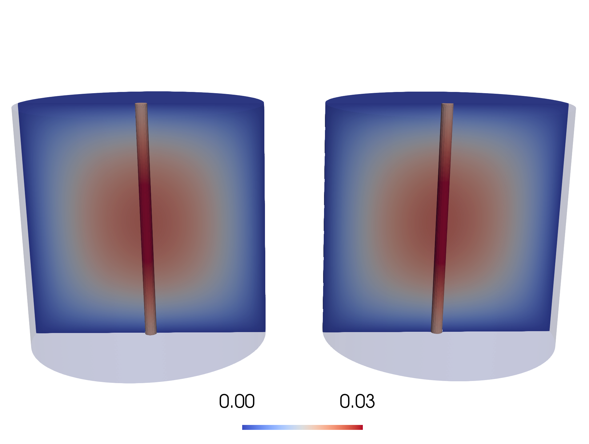
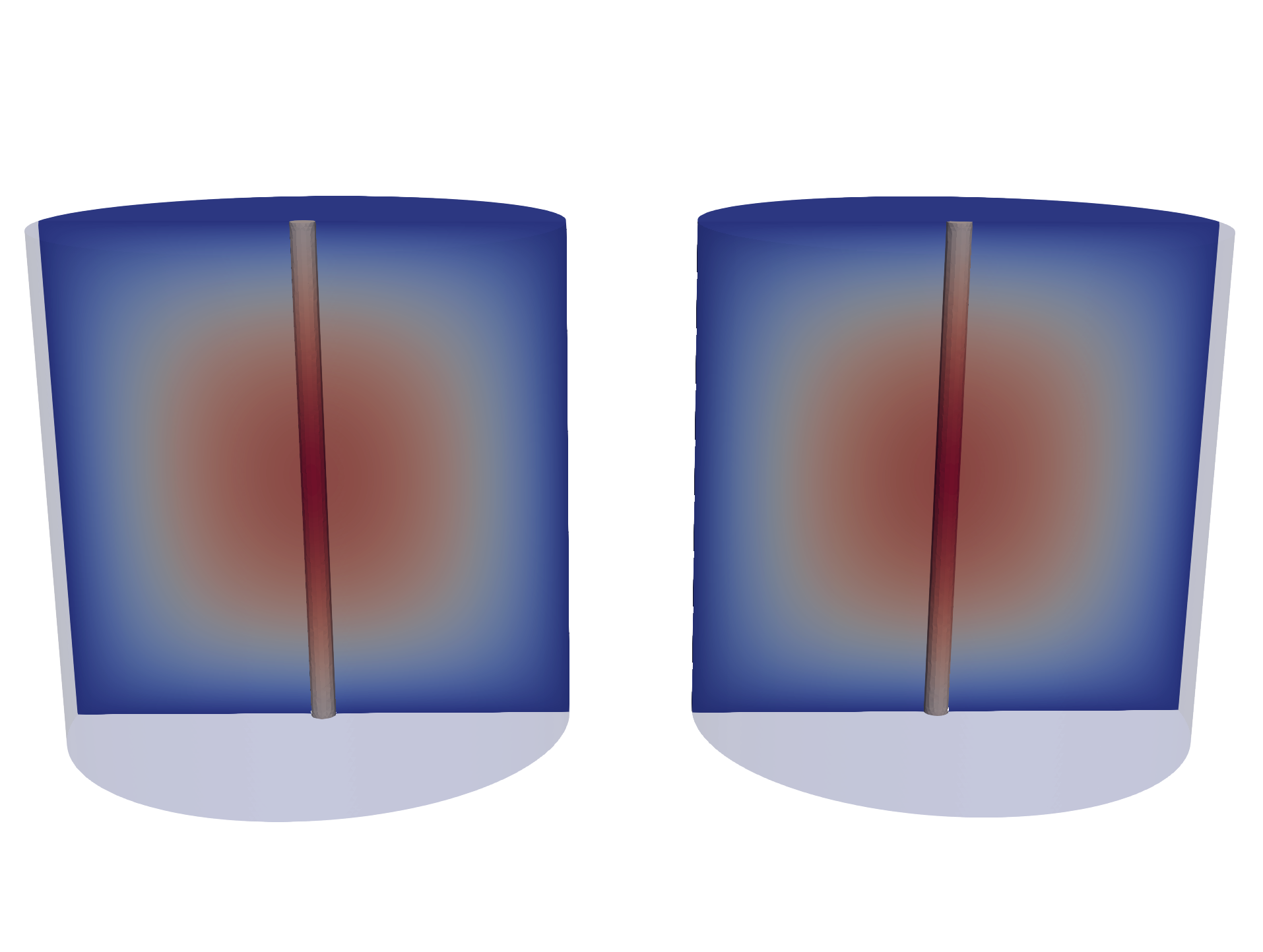
Figure 4. Plot of the numerical solutions for the first example with $R=0.0125$. The 3D-3D solution $(c_{s,\tau h},c_{v,\tau h})$ is plotted next to the 3D-1D model $(c_{\tau,h},E\hat{c}_{\tau h})$ with the 1D solution extended to the inner cylinder. The outer cylinder is clipped at the plane intersecting the center line $\Lambda$. (Left) Solutions shown at $t=0.1$. (Right) Solutions shown at $t=T=0.2$.

To numerically explore the modelling error for decreasing radii ($R$, $\epsilon_{\max}\rightarrow 0$), we consider a series of experiments with different radii $R\in\{0.2,0.1,0.05,0.025,0.0125\}$, a relatively small, fixed mesh size $(h_{\min},h_{\max})|_{\Omega_{v}}=(0.009,0.014)$ and $(h_{\min},h_{\max})|_{\Omega_{s}}=(0.01,0.024)$, and small, fixed time step $\tau=0.01$. In practice, we compute the discrepancy between the approximate solutions in the 3D and 1D vessels:

$$\|c_{v,\tau h}(T)-E\hat{c}_{\tau h}(T)\|_{L^{2}(\Omega_{v})}\approx\|c_{v}(T)-E\hat{c}(T)\|_{L^{2}(\Omega_{v})}$$

as a proxy for the modelling error while noting that the computed error includes both the spatio-temporal approximation errors as well as modelling errors:

$$\|c_{v}(T)-\hat{c}(T)\|_{L^{2}(\Omega_{v})}\\ \leq\|c_{v}(T)-c_{v,\tau h}(T)\|_{L^{2}(\Omega_{v})}+\|c_{v,\tau h}(T)-\hat{c}_{\tau h}(T)\|_{L^{2}(\Omega_{v})}+\|\hat{c}(T)-\hat{c}_{\tau h}(T)\|_{L^{2}(\Omega_{v})}.$$

We here thus presume that with the choice of small mesh size and time step, the approximation errors are negligible compared to the modelling error.

Table 1 shows the computed $L^{2}$ norms in $\Omega_{v}$ and $\Omega_{s}$ along with normalized norms and the corresponding rates. We observe that the errors decrease with decreasing $R$ until the radius and mesh size become of comparable size, and that the modelling error in the surroundings continues to decrease even when the modelling error in the vessel stagnates.

$R$	$E_{v}$	rate	$\tilde{E}_{v}$	rate	$E_{s}$	rate
0.1	4.405e-04	-	2.485e-03	-	4.426e-04	-
0.05	5.244e-05	3.07	5.918e-04	2.07	1.375e-04	1.69
0.025	1.394e-05	1.91	3.146e-04	0.91	3.636e-05	1.92
0.0125	7.806e-06	0.84	3.523e-04	-0.16	9.738e-06	1.90

Table 1. Numerical example 1: Model errors $E_{v}=\|c_{v,\tau h}(T)-\hat{c}_{\tau,h}(T)\|_{L^{2}(\Omega_{v})}$ and $\tilde{E}_{v}=|\Omega_{v}|^{-1/2}\|c_{v,\tau h}(T)-\hat{c}_{\tau,h}(T)\|_{L^{2}(\Omega_{v})}$ in a vessel $\Omega_{v}$ of varying radius $R$, and in the surroundings $E_{s}=\|c_{s,\tau h}(T)-c_{h}(T)\|_{L^{2}(\Omega_{s})}$.

8.2. A coupled 3D-1D-1D solute transport example

As a second example, we consider solutions to the coupled 3D-1D-1D models of solute transport and the corresponding 3D-3D-3D model set up in the blood vessel, $\Omega_{v}$, the perivascular domain $\Omega_{p}$, and the tissue $\Omega_{s}$. We also use backward Euler and continuous linear finite element methods to solve (5.3)-(5.5) with solutions denoted by $(c_{\tau h},\hat{c}_{p,\tau h},\hat{c}_{v,\tau h})$, and the corresponding 3D-3D-3D model with solutions denoted by $(c_{s,\tau h},c_{p,\tau h},c_{v,\tau h})$. We set $\Omega_{s}=(-1,1)\times(-1,1)\times(-0.5,0.5)$, $\Omega_{v}$ be a cylinder of radius $R_{1}$ with centerline $x=0$, $y=0$, $\Omega_{p}$ be the annular cylinder around $\Omega_{v}$ with outer radius $R_{2}=2R_{1}$ . We vary $R_{1}$ and compute the $L^{2}$ error between the 3D solutions $c_{i,\tau h}$ and the reduced 1D solutions $\hat{c}_{i,\tau h}$ for $i\in\{p,v\}$. We keep $\tau=0.01$ and $T=0.1$, $D_{v}=D_{p}=D_{s}=\xi_{v}=\xi_{p}=1$, $f_{s}=f_{v}=f_{p}=0.5$, $c_{v,\tau h}=\hat{c}_{v,\tau h}(0)=1.0$, $c_{p,\tau h}=\hat{c}_{p,\tau h}(0)=c_{\tau h}(0)=c_{s,\tau h}(0)=0$, $\boldsymbol{u}_{v}=(0.5,0,0)$, $\boldsymbol{u}_{p}=(0.1,0,0)$, and $\boldsymbol{u}_{s}=(0.05,0,0)$. For the mesh–size in the variuous domains, we have $(h_{\min},h_{\max})|_{\Omega_{v}}=(0.011,0.019)$, $(h_{\min},h_{\max})|_{\Omega_{p}}=(0.011,0.024)$, and $(h_{\min},h_{\max})|_{\Omega_{s}}=(0.017,0.043)$.

Tables 2 and 3 show the computed $L^{2}$ norm in $\Omega_{v}$, $\Omega_{p}$ and $\Omega_{s}$ along with a normalized norm and the corresponding rates. We observe that the modelling errors all decrease for decreasing radii, though in a non-uniform manner and with uneven rates. The modeling error in the surroundings decreases robustly at rates between 1 and 2. The (non-normalized) modelling error in the vascular domain decreases with similar rates. The modelling error in the perivascular space increases in the first $R$-refinement before decreasing at rates close to $2$. Clearly, further theoretical and numerical studies of the interplay between the modelling and approximation errors are warranted (though outside the scope of the current study).

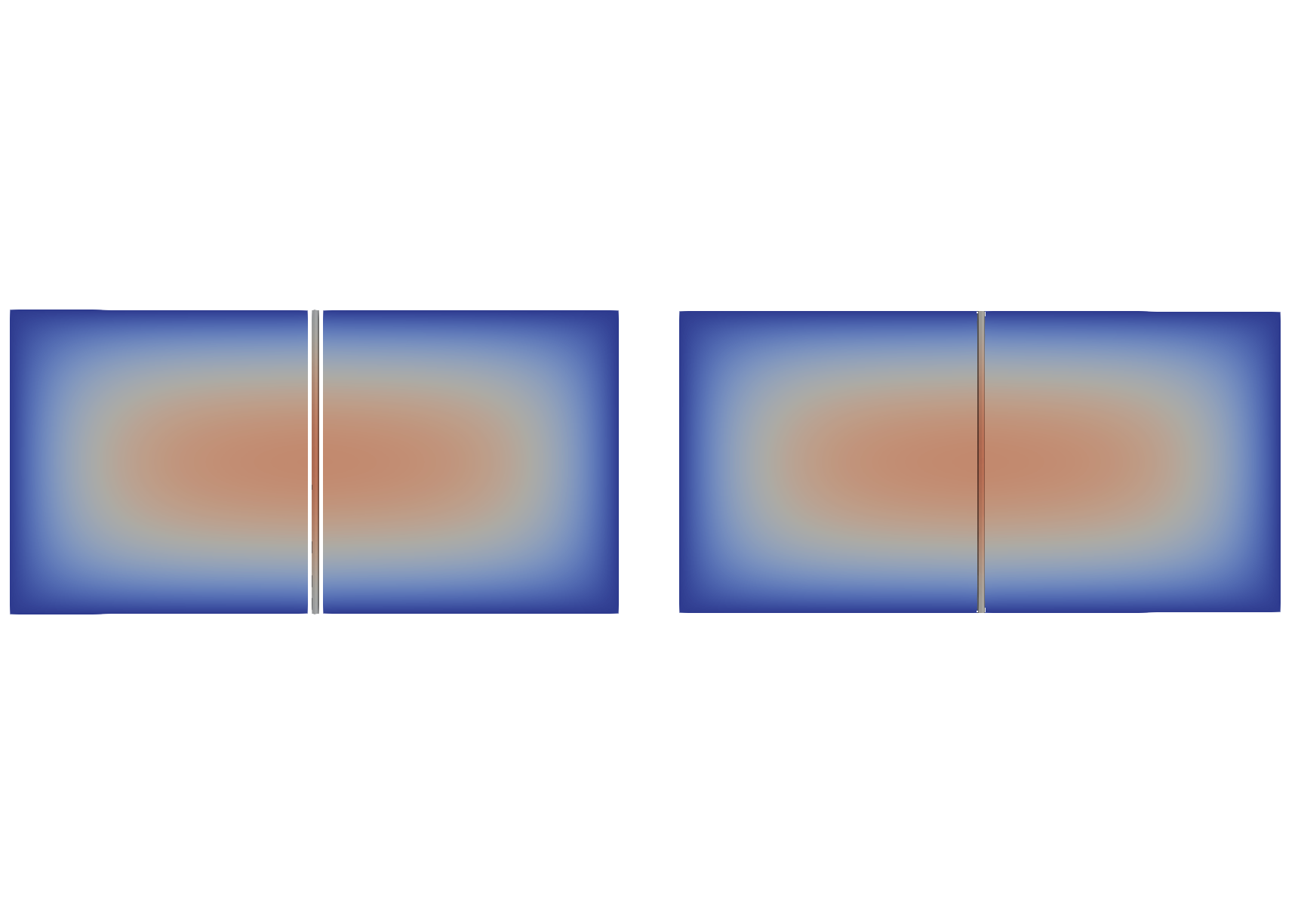
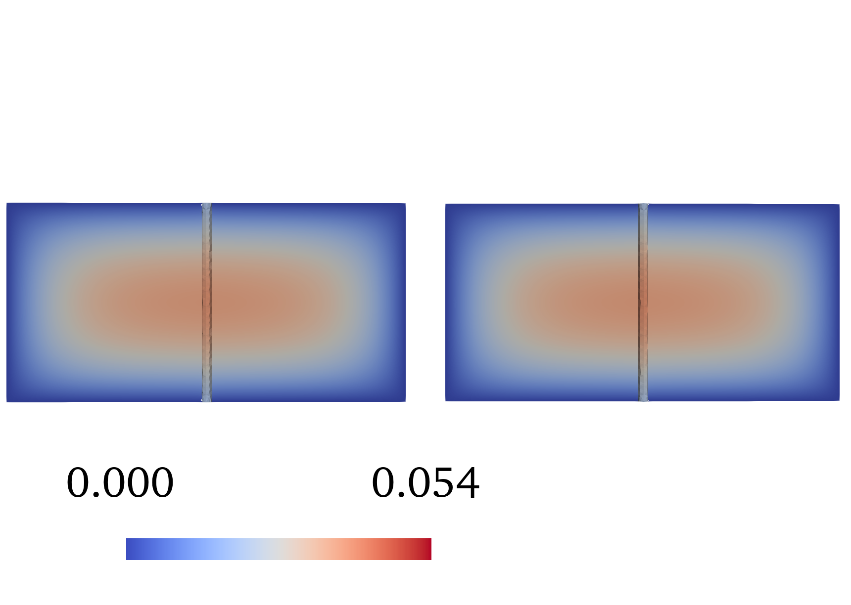
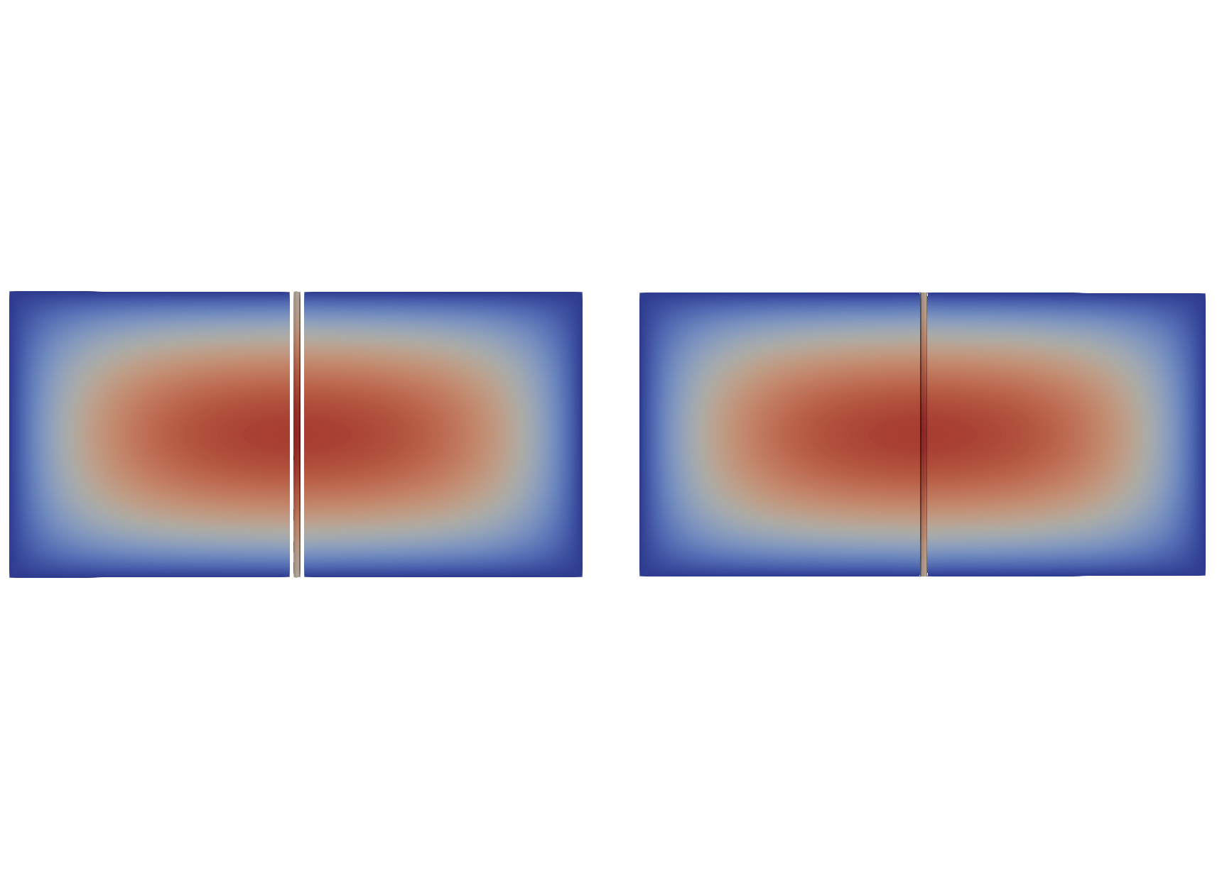
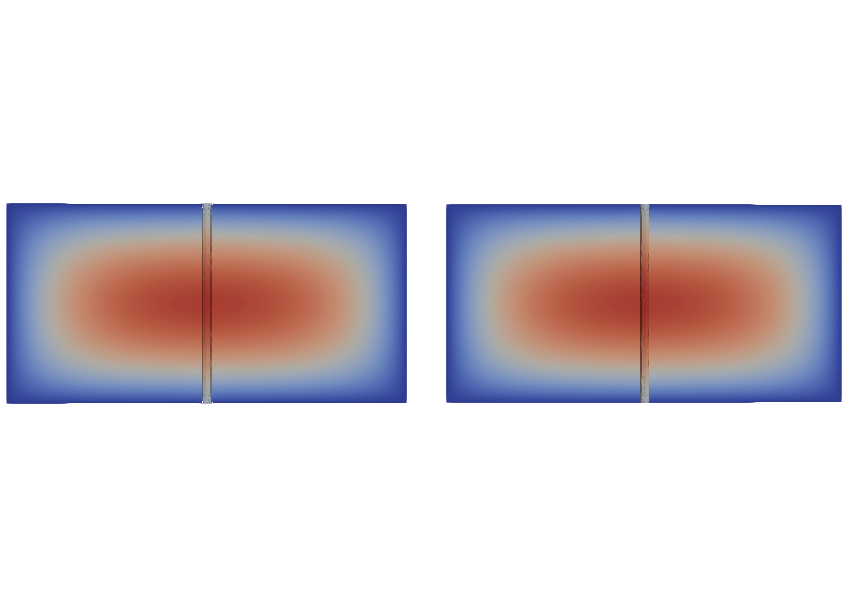
Figure 5. Plot of the numerical solutions for the second example with $R=0.0125$. In each of the four quadrants, the 3D-3D-3D solution $(c_{s,\tau h},c_{p,\tau h},c_{v,\tau h})$ is plotted next to the 3D-1D-1D model $(c_{\tau h},\hat{c}_{p,\tau h},\hat{c}_{v,\tau h})$ with the 1D solutions extended to their respective cylinder or annulus. Top row shows a slice of $\Omega_{s}$ and $\Omega$ respectively with the vessel solutions without the PVS domain. The second row shows the PVS solution. (Left) Solutions shown at $t=0.1$. (Right) Solutions shown at $t=T=0.2$.

$R_{1}$	$E_{v,2}$	rate	$\tilde{E}_{v,2}$	rate	$E_{p}$	rate	$\tilde{E}_{p}$	rate
0.1	2.195e-03	–	1.239e-02	–	1.698e-03	–	4.790e-03	–
0.05	1.902e-04	3.53	2.146e-03	2.53	1.609e-04	3.40	9.077e-04	2.40
0.025	3.243e-05	2.55	7.319e-04	1.55	2.950e-05	2.48	3.329e-04	1.48
0.0125	1.507e-05	1.10	6.803e-04	0.10	2.162e-05	0.49	4.880e-04	-0.55

Table 2. Numerical example 2: Model errors $E_{v,2}=\|c_{v,\tau h}-E\hat{c}_{v,\tau h}\|_{L^{2}(\Omega_{v})}$, $\tilde{E}_{v,2}=|\Omega_{v}|^{-1/2}\|c_{v,\tau h}-E\hat{c}_{v,\tau h}\|_{L^{2}(\Omega_{v})}$,$E_{p}=\|c_{p,\tau h}-E\hat{c}_{p,\tau h}\|_{L^{2}(\Omega_{p})}$, and $\tilde{E}_{p}=|\Omega_{v}|^{-1/2}\|c_{p,\tau h}-E\hat{c}_{p,\tau h}\|_{L^{2}(\Omega_{p})}$ of varying radius $R_{1}$. Note that the smallest $R_{1}$ is of the order of $h_{\min}$ in $\Omega_{v}$

$R_{2}$	$\|c_{\tau h}(T)-c_{s,\tau h}(T)\|_{L^{2}(\Omega_{s})}$	rate
0.2	9.816e-04	–
0.1	1.762e-04	2.48
0.05	6.869e-05	1.36
0.025	3.693e-05	0.89

Table 3. Numerical example 2: Model error in the surrounding domain $\Omega_{s}$.

9. Conclusions and outlook

Understanding solute transport and exchange in the brain vasculature, perivasculature, and surrounding tissue is critical for unraveling the brain’s delivery and clearance mechanisms. Here, we have presented a mathematical model for modelling diffusive and convective transport and exchange in deformable domains, and rigorously analyzed its modelling characteristics. Future research directions include the error analysis of conforming and non-conforming finite element approximations of such models. We easily envision that this framework can be combined with medical imaging to study brain perivascular transport and exchange at scale.

Appendix A Technical estimates

A.1. Uniform bound on $C_{1},C_{2}$ and $N_{2}$ as defined in Propositions 7.1 and 7.2

We derive a bound independent of $\epsilon_{\max}$ on $C_{1}+C_{2}$ under the assumption that $\partial_{t}c\in L^{2}(0,T;L^{2}(\Omega))$ and $\partial_{t}\hat{c}\in L^{2}(0,T;L^{2}_{A}(\Lambda))$ which follow from maximal regularity, see Proposition 4.2. From the definitions of $C_{1}$ and $C_{2}$, it suffices to obtain a bound on:

(A.1) $$W_{1} =\|\hat{c}\|_{L^{2}(0,T;H^{1}(\Omega_{v}(t)))}+\|c\|_{L^{2}(0,T;H^{1}(\Omega))}+\|\hat{c}\|_{L^{2}(0,T;L^{2}(\partial\Omega_{v}(t)))}+\|\overline{c}\|_{L^{2}(0,T;L^{2}(\Gamma(t)))},$$

(A.2) $$W_{2} =\|c_{s}\|_{L^{2}(0,T;H^{1}(\Omega_{s}(t)))}+\|\overline{c_{s}}\|_{L^{2}(0,T;L^{2}(\Gamma(t)))}.$$

We will make use of the following estimate. With Cauchy-Schwarz inequality, we have that

(A.3) $$b_{\Lambda}(v,w)\leq\|\xi^{1/2}v\|_{L^{2}_{P}(\Lambda)}\|\xi^{1/2}w\|_{L^{2}_{P}(\Lambda)},\quad\forall v,w\in L^{2}_{P}(\Lambda).$$

In (4.20a), choose $v=c$. We obtain

(A.4) $$\frac{1}{2}\int_{\Omega}\partial_{t}c^{2}+\tilde{\nu}\|\nabla c\|^{2}_{L^{2}(\Omega)}+\|\xi^{1/2}\bar{c}\|_{L_{P}^{2}(\Lambda)}^{2}=(\mathcal{E}\boldsymbol{u}_{s}c,\nabla c)_{\Omega}+b_{\Lambda}(\hat{c},\bar{c})+(\mathcal{E}f_{s},c)_{\Omega}.$$

With Hölder’s inequality and (A.3), we obtain

$$\frac{1}{2}\int_{\Omega}\partial_{t}c^{2}+\tilde{\nu}\|\nabla c\|^{2}_{L^{2}(\Omega)}+\|\xi^{1/2}\bar{c}\|_{L_{P}^{2}(\Lambda)}^{2}\leq\|\mathcal{E}\boldsymbol{u}_{s}\|_{L^{\infty}(\Omega)}\|c\|_{L^{2}(\Omega)}\|\nabla c\|_{L^{2}(\Omega)}$$

$$+\|\xi^{1/2}\hat{c}\|_{L^{2}_{P}(\Lambda)}\|\xi^{1/2}\bar{c}\|_{L^{2}_{P}(\Lambda)}+\|\mathcal{E}f_{s}\|_{L^{2}(\Omega)}\|c\|_{L^{2}(\Omega)}.$$

Applying Young’s inequality and multiplying by $2$ yields:

(A.5) $$\int_{\Omega}\partial_{t}c^{2}+\tilde{\nu}\|\nabla c\|^{2}_{L^{2}(\Omega)}+\|\xi^{1/2}\bar{c}\|_{L_{P}^{2}(\Lambda)}^{2}\\ \leq(1+\tilde{\nu}^{-1}\|\mathcal{E}\boldsymbol{u}_{s}\|^{2}_{L^{\infty}(\Omega)})\|c\|^{2}_{L^{2}(\Omega)}+\|\xi^{1/2}\hat{c}\|^{2}_{L^{2}_{P}(\Lambda)}+\|\mathcal{E}f_{s}\|^{2}_{L^{2}(\Omega)}.$$

Next, choose $v=\hat{c}$ in (4.20b). Since $\langle\hat{c}\rangle=\bar{\hat{c}}=\hat{c}$, we have

(A.6) $$\int_{\Lambda}\partial_{t}(A\hat{c})\hat{c}+\|D_{v}^{1/2}\partial_{s}\hat{c}\|_{L^{2}(\Omega_{v})}^{2}+\|\xi^{1/2}\hat{c}\|^{2}_{L^{2}_{P}(\Lambda)}=(\hat{c}U,\partial_{s}\hat{c})_{\Omega_{v}}+b_{\Lambda}(\hat{c},\bar{c})+(\langle f_{v}\rangle,\hat{c})_{\Omega_{v}}.$$

In the above, it is implicitly understood that $\hat{c}=E\hat{c}$. Similarly, with Hölder’s and Young’s inequalities, we have

(A.7) $$2\int_{\Lambda}\partial_{t}(A\hat{c})\hat{c}+\|D_{v}^{1/2}\partial_{x}\hat{c}\|_{L^{2}(\Omega_{v})}^{2}+\|\xi^{1/2}\hat{c}\|^{2}_{L^{2}_{P}(\Lambda)}\\ \leq(1+\|D_{v}^{-1/2}U\|^{2}_{L^{\infty}(\Omega_{v})})\|\hat{c}\|^{2}_{L^{2}(\Omega_{v})}+\|\xi^{1/2}\bar{c}\|_{L_{P}^{2}(\Lambda)}^{2}+\|\langle f_{v}\rangle\|_{L^{2}(\Omega_{v})}^{2}.$$

Observe that with Reynolds transport theorem, we have that

(A.8) $$\int_{\Lambda}\partial_{t}(A\hat{c})\hat{c}=\int_{\Lambda}\partial_{t}(A\hat{c}^{2})-\frac{1}{2}\int_{\Lambda}A\partial_{t}\hat{c}^{2}=\partial_{t}\int_{\Lambda}(A\hat{c}^{2})-\frac{1}{2}\int_{\Omega_{v}(t)}\partial_{t}\hat{c}^{2}$$

$$=\frac{1}{2}\partial_{t}\int_{\Omega_{v}(t)}\hat{c}^{2}+\frac{1}{2}\int_{\Lambda}\hat{c}^{2}\int_{\partial\Theta}\boldsymbol{w}\cdot\boldsymbol{n}=\frac{1}{2}\partial_{t}\int_{\Omega_{v}(t)}\hat{c}^{2}+\frac{1}{2}\int_{\Lambda}\hat{c}^{2}\int_{\Theta}\nabla\cdot\boldsymbol{w}$$

$$=\frac{1}{2}\partial_{t}\int_{\Omega_{v}(t)}\hat{c}^{2}+\frac{1}{2}\int_{\Omega_{v}(t)}\hat{c}^{2}\nabla\cdot\boldsymbol{w}.$$

Adding (A.5) and (A.7) with using (A.8), and integrating from $0,t$, we obtain

$$\|c(t)\|^{2}_{L^{2}(\Omega)}+\|\hat{c}(t)\|_{L^{2}(\Omega_{v})}^{2}+\tilde{\nu}\|\nabla c\|_{L^{2}(0,t;L^{2}(\Omega))}^{2}+\|D_{v}^{1/2}\partial_{s}\hat{c}\|_{L^{2}(0,t;L^{2}(\Omega_{v}))}^{2}$$

$$\leq\|\mathcal{E}f_{s}\|_{L^{2}(0,t;L^{2}(\Omega))}^{2}+\|\langle f_{v}\rangle\|_{L^{2}(0,t;L^{2}(\Omega_{v}))}^{2}+\|c^{0}\|^{2}_{L^{2}(\Omega)}+\|\hat{c}^{0}\|^{2}_{L^{2}(\Omega_{v})}$$

$$+(1+\tilde{\nu}^{-1}\|\mathcal{E}\boldsymbol{u}_{s}\|^{2}_{L^{\infty}(0,T;L^{\infty}(\Omega))})\|c\|^{2}_{L^{2}(0,t;L^{2}(\Omega_{v}))}$$

$$+(1+\|D_{v}^{-1/2}U\|^{2}_{L^{\infty}(0,T;L^{\infty}(\Omega_{v}))}+\|\nabla\cdot\boldsymbol{w}\|_{L^{\infty}(0,T;L^{\infty}(\Omega))})\|\hat{c}\|^{2}_{L^{2}(0,t;L^{2}(\Omega_{v}))}.$$

With continuous Gronwall’s inequality, we obtain

(A.9) $$\|c\|_{L^{\infty}(0,T;L^{2}(\Omega))}^{2}+\|\hat{c}\|_{L^{\infty}(0,T;L^{2}(\Omega_{v}))}^{2}+\tilde{\nu}\|\nabla c\|_{L^{2}(0,T;L^{2}(\Omega))}^{2}+\|D_{v}^{1/2}\partial_{s}\hat{c}\|_{L^{2}(0,T;L^{2}(\Omega_{v}))}^{2}\leq K.$$

Here, $K$ depends on the final time $T$, the velocities $\boldsymbol{u}_{s}$ and $U$, the initial conditions, and the source terms, but not on $|\Omega_{v}|$. Further, from (6.16) and with the above bound, we have

(A.10) $$\|\overline{c}\|_{L^{2}(0,T;L^{2}_{P}(\Lambda))}\leq\|c\|_{L^{2}(0,T;L^{2}(\Gamma))}\leq K_{\Gamma}\epsilon^{1/6}\|c\|^{2}_{L^{2}(0,T;H^{1}(\Omega))}\leq K.$$

We then use the above in (A.7) after integrating over time. With Gronwall’s inequality, we can conclude the bound

(A.11) $$\|\hat{c}\|_{L^{2}(0,T;L^{2}(\Gamma))}^{2}\leq K.$$

To obtain a bound on $\|\hat{c}\|_{L^{2}(0,T;L^{2}(\partial\Omega_{v}))}$, we first note that since $\hat{c}$ is uniform on each cross-section:

(A.12) $$\|\hat{c}\|^{2}_{L^{2}(\partial\Omega_{v})}=\|\hat{c}\|_{L^{2}(\Gamma)}^{2}+\int_{\Lambda}\int_{\partial\Theta_{1}}\hat{c}^{2}=\|\hat{c}\|_{L^{2}(\Gamma)}^{2}+\int_{\Lambda}\hat{c}^{2}|\partial\Theta_{1}|\\ =\|\hat{c}\|_{L^{2}(\Gamma)}^{2}+\int_{\Lambda}\frac{|\partial\Theta_{1}|}{|\partial\Theta_{2}|}\int_{\Theta_{2}}\hat{c}^{2}\lesssim\|\hat{c}\|_{L^{2}(\Gamma)}^{2}\lesssim K.$$

The above follows by the assumption on the radii $R_{1}$ and $R_{2}$ (6.3). Thus, $W_{1}$ is bounded independent of $\epsilon_{\max}$. For the original 3D-3D problem, choose $\boldsymbol{\phi}=(c_{v},c_{s})$ in (3.11) and use (3.13). We obtain that

(A.13) $$\langle\dot{c_{v}},c_{v}\rangle_{H^{-1}(\Omega_{v}(t))}+(\nabla\cdot\boldsymbol{w}c_{v},c_{v})_{\Omega_{v}(t)}+\langle\dot{c_{s}},c_{s}\rangle_{H^{-1}(\Omega_{s}(t))}+(\nabla\cdot\boldsymbol{w}c_{s},c_{s})_{\Omega_{s}(t)}\\ +K_{1}(\|c_{v}\|_{H^{1}(\Omega_{v}(t))}^{2}+\|c_{s}\|_{H^{1}(\Omega_{s}(t))}^{2})\leq(K_{2}+1)(\|c_{v}\|_{L^{2}(\Omega_{v}(t))}^{2}+\|c_{s}\|_{L^{2}(\Omega_{s}(t))}^{2})+\|f_{v}\|^{2}_{L^{2}(\Omega_{v})}+\|f_{s}\|^{2}_{L^{2}(\Omega_{s})}.$$

Note that the constants $K_{1}$ and $K_{2}$ are independent of $\epsilon$. With [3, Corollary 2.41] for $i\in\{v,s\}$:

(A.14) $$\int_{0}^{t}\langle\dot{c_{i}},c_{i}\rangle_{H^{-1}(\Omega_{i}(t))}=\frac{1}{2}(\|c_{i}(t)\|_{L^{2}(\Omega_{i}(t))}^{2}-\|c_{i}(0)\|_{L^{2}(\Omega_{i}(0))}^{2})-\int_{0}^{t}\frac{1}{2}(\nabla\cdot\boldsymbol{w}c_{i},c_{i})_{\Omega_{i}(t)},$$

we obtain:

(A.15) $$\frac{1}{2}( \|c_{v}(t)\|^{2}_{L^{2}(\Omega_{v}(t))}+\|c_{s}(t)\|^{2}_{L^{2}(\Omega_{s}(t))})+K_{1}(\|c_{v}\|_{L^{2}(0,t;H^{1}(\Omega_{v}(t)))}^{2}+\|c_{s}\|_{L^{2}(0,t;H^{1}(\Omega_{s}(t)))}^{2})$$

$$\leq(K_{2}+1+\|\nabla\cdot\boldsymbol{w}\|_{L^{\infty}(0,t;L^{\infty}(\Omega))})(\|c_{v}\|_{L^{2}(0,t;L^{2}(\Omega_{v}(t)))}^{2}+\|c_{s}\|_{L^{2}(0,t;L^{2}(\Omega_{s}(t)))}^{2})$$

$$\,\,\,\,\,+\frac{1}{2}(\|c_{v}(0)\|^{2}_{L^{2}(\Omega_{v}(0))}+\|c_{s}(0)\|^{2}_{L^{2}(\Omega_{s}(0))})+\|f_{v}\|^{2}_{L^{2}(0,t;L^{2}(\Omega_{v}))}+\|f_{s}\|^{2}_{L^{2}(0,t;L^{2}((\Omega_{s})))}.$$

With Gronwall’s inequality, we can then conclude that:

(A.16) $$\|c_{v}\|_{L^{\infty}(0,T;L^{2}(\Omega_{v}(t)))}^{2}+\|c_{s}\|_{L^{\infty}(0,T;L^{2}(\Omega_{s}(t)))}^{2}\\ +\|c_{v}\|_{L^{2}(0,T;H^{1}(\Omega_{v}(t)))}^{2}+\|c_{s}\|_{L^{2}(0,T;H^{1}(\Omega_{s}(t)))}^{2}\leq K.$$

Similar to the arguments above, we use trace estimate (6.16) to conclude that

(A.17) $$\|\overline{c_{s}}\|_{L^{2}(0,T;L^{2}(\Gamma))}\leq\|c_{s}\|_{L^{2}(0,T;L^{2}(\Gamma))}\leq K.$$

Thus, $W_{2}$ is bounded which concludes the argument that $W$ is bounded independent of $\epsilon_{\max}$. Then, we use the above bound in the energy inequality for $c_{v}$ (which can be obtained by choosing $\boldsymbol{\phi}=(c_{v},0)$ in (3.11)) to obtain that

(A.18) $$\|c_{v}\|_{L^{2}(0,T;L^{2}(\Gamma))}\leq K.$$

This shows that $N_{2}$, as defined in Proposition 7.2 is bounded independent of $\epsilon_{\max}$.

A.2. Hölder continuity bound

We verify that the terms involving $b_{\Lambda}$ in $\mathcal{A}_{\Lambda}(t,\cdot,\cdot)$ satisfy the bound stated in (4.25). We focus on the following term as it is the most intricate:

(A.19) $$b_{\Lambda}(\overline{c}(t_{1}) ,\overline{v}(t_{1}))-b_{\Lambda}(\overline{c}(t_{2}),\overline{v}(t_{2}))=\int_{\Gamma(t_{2})}\xi(t_{2})c\overline{v}(t_{2})-\int_{\Gamma(t_{1})}\xi(t_{1})c\overline{v}(t_{1})$$

$$=\int_{\Gamma(t_{2})}(\xi(t_{2})-\xi(t_{1}))c\overline{v}(t_{2})+\left(\int_{\Gamma(t_{2})}\xi(t_{1})c\overline{v}(t_{2})-\int_{\Gamma(t_{1})}\xi(t_{1})c\overline{v}(t_{2})\right)$$

$$+\int_{\Gamma(t_{1})}\xi(t_{1})c\left(\overline{v}(t_{2})-\overline{v}(t_{1})\right)=T_{1}+T_{2}+T_{3}.$$

For the first term, the Hölder continuity bound follows form the assumption on $\xi$, the observation that $\|\overline{v}\|_{L^{2}(\Gamma(t_{2}))}\leq\|v\|_{L^{2}(\Gamma(t_{2}))}$, and from (3.15). Indeed, we have that

(A.20) $$\int_{\Gamma(t_{2})}(\xi(t_{2})-\xi(t_{1}))c\overline{v}(t_{2}) \leq\|\xi(t_{2})-\xi(t_{2})\|_{L^{\infty}(\Lambda)}\|c\|_{L^{2}(\Gamma(t_{2}))}\|\overline{v}\|_{L^{2}(\Gamma(t_{2}))}$$

$$\leq C|t_{2}-t_{1}|^{\beta}\|c\|_{H^{1}(\Omega)}\|v\|_{H^{1}(\Omega)}.$$

To handle the second term in (A.19), observe that the specific domains of section 2.2 allow us to write

$$T_{2}=\int_{\Lambda}\int_{0}^{2\pi}(R_{2}(t_{2})-R_{2}(t_{1}))\xi(t_{1})c\overline{v}(t_{2})\leq C|t_{2}-t_{1}|^{\beta}\|c\|_{L^{2}(\Gamma(0))}\|\overline{v}(t_{2})\|_{L^{2}(\Gamma(0))}\\ \leq C|t_{2}-t_{1}|^{\beta}\|c\|_{H^{1}(\Omega)}\|v\|_{H^{1}(\Omega)}.$$

In the above, we assumed without loss of generality that $\partial\Theta_{2}(0)$ has radius $1$, and we use that $R_{2}$ is Hölder continuous. For $T_{3}$, we have for a.e in $\Lambda$

$$|\overline{v}(t_{2})-\overline{v}(t_{1})|=\left(\frac{1}{P(t_{2})}-\frac{1}{P(t_{1})}\right)\int_{0}^{2\pi}R_{2}(t_{2})v+\frac{1}{P(t_{1})}\int_{0}^{2\pi}(R_{2}(t_{2})-R_{2}(t_{1}))v$$

$$\leq\left\|\frac{1}{P(t_{2})}-\frac{1}{P(t_{1})}\right\|_{L^{\infty}(\Lambda)}\|R_{2}(t_{2})\|_{L^{2}(\partial\Theta_{2}(0))}\|v\|_{L^{2}(\partial\Theta_{2}(0))}$$

$$\quad+\left\|\frac{1}{P(t_{1})}\right\|_{L^{\infty}(\Lambda)}\|R_{2}(t_{2})-R_{2}(t_{1})\|_{L^{2}(\partial\Theta_{2}(0))}\|v\|_{L^{2}(\partial\Theta_{2}(0))}.$$

Hence, $T_{3}$ is bounded as follows:

$$T_{3}\leq\|c\|_{L^{2}(\Gamma(t_{1}))}\|\overline{v}(t_{2})-\overline{v}(t_{1})\|_{L^{2}(\Gamma(t_{1}))}\leq C|t_{2}-t_{1}|^{\beta}\|c\|_{H^{1}(\Omega)}\|v\|_{H^{1}(\Omega)},$$

where we used the Hölder continuity assumptions of $P^{-1}$ and on $R_{2}$ with follow from the smoothness assumptions on the domain velocity $\boldsymbol{w}\in C^{2}$. The other terms with $b_{\Lambda}$ can be handled similarly.

References

- [1] N. J. Abbott. Evidence for bulk flow of brain interstitial fluid: significance for physiology and pathology. Neurochemistry International, 45(4):545–552, 2004.
- [2] M. Alnæs, J. Blechta, J. Hake, A. Johansson, B. Kehlet, A. Logg, C. Richardson, J. Ring, M. E. Rognes, and G. N. Wells. The FEniCS project version 1.5. Archive of Numerical Software, 3(100), 2015.
- [3] A. Alphonse, C. M. Elliott, and B. Stinner. An abstract framework for parabolic PDEs on evolving spaces. Portugaliae Mathematica, 72(1):1–46, 2015.
- [4] W. Arendt, D. Dier, and S. Fackler. JL Lions’ problem on maximal regularity. Archiv der Mathematik, 109(1):59–72, 2017.
- [5] W. F. Boron and E. L. Boulpaep. Medical Physiology. Elsevier Health Sciences, 2012.
- [6] S. C. Brenner and L. R. Scott. The Mathematical Theory of Finite Element Methods, volume 3. Springer, 2008.
- [7] H. Brezis. Functional Analysis, Sobolev Spaces and Partial Differential Equations, volume 2. Springer, 2010.
- [8] T. Brinker, E. Stopa, J. Morrison, and P. Klinge. A new look at cerebrospinal fluid circulation. Fluids and Barriers of the CNS, 11(1):1–16, 2014.
- [9] S. Čanić and E. H. Kim. Mathematical analysis of the quasilinear effects in a hyperbolic model blood flow through compliant axi-symmetric vessels. Mathematical Methods in the Applied Sciences, 26(14):1161–1186, 2003.
- [10] M. Causemann, V. Vinje, and M. E. Rognes. Human intracranial pulsatility during the cardiac cycle: a computational modelling framework. Fluids and Barriers of the CNS, 19(1):1–17, 2022.
- [11] C. D’Angelo. Multiscale modelling of metabolism and transport phenomena in living tissues. Technical report, EPFL, 2007.
- [12] C. D’Angelo. Finite element approximation of elliptic problems with Dirac measure terms in weighted spaces: applications to one-and three-dimensional coupled problems. SIAM Journal on Numerical Analysis, 50(1):194–215, 2012.
- [13] C. D’angelo and A. Quarteroni. On the coupling of 1D and 3D diffusion-reaction equations: application to tissue perfusion problems. Mathematical Models and Methods in Applied Sciences, 18(08):1481–1504, 2008.
- [14] C. Daversin-Catty, I. G. Gjerde, and M. E. Rognes. Geometrically reduced modelling of pulsatile flow in perivascular networks. Frontiers in Physics, page 360, 2022.
- [15] C. Daversin-Catty, V. Vinje, K.-A. Mardal, and M. E. Rognes. The mechanisms behind perivascular fluid flow. Plos one, 15(12):e0244442, 2020.
- [16] M. C. Delfour and J.-P. Zolésio. Shapes and Geometries: Metrics,Analysis, Differential Calculus, and Optimization. SIAM, 2011.
- [17] E. Di Nezza, G. Palatucci, and E. Valdinoci. Hitchhiker’s guide to the fractional Sobolev spaces. Bulletin des Sciences Mathématiques, 136(5):521–573, 2012.
- [18] L. C. Evans. Partial Differential Equations, volume 19. American Mathematical Society, 2010.
- [19] G. J. Fleischman, T. W. Secomb, and J. F. Gross. The interaction of extravascular pressure fields and fluid exchange in capillary networks. Mathematical Biosciences, 82(2):141–151, 1986.
- [20] L. Formaggia, J.-F. Gerbeau, F. Nobile, and A. Quarteroni. On the coupling of 3D and 1D Navier–Stokes equations for flow problems in compliant vessels. Computer Methods in Applied Mechanics and Engineering, 191(6-7):561–582, 2001.
- [21] I. G. Gjerde, K. Kumar, and J. M. Nordbotten. A singularity removal method for coupled 1D–3D flow models. Computational Geosciences, 24(2):443–457, 2020.
- [22] I. G. Gjerde, K. Kumar, J. M. Nordbotten, and B. Wohlmuth. Splitting method for elliptic equations with line sources. ESAIM: Mathematical Modelling and Numerical Analysis, 53(5):1715–1739, 2019.
- [23] W. Gong, G. Wang, and N. Yan. Approximations of elliptic optimal control problems with controls acting on a lower dimensional manifold. SIAM Journal on Control and Optimization, 52(3):2008–2035, 2014.
- [24] J.-L. Guermond and A. Ern. Finite Elements I: Approximation and Interpolation. Springer, 2021.
- [25] M.-J. Hannocks, M. E. Pizzo, J. Huppert, T. Deshpande, N. J. Abbott, R. G. Thorne, and L. Sorokin. Molecular characterization of perivascular drainage pathways in the murine brain. Journal of Cerebral Blood Flow & Metabolism, 38(4):669–686, 2018.
- [26] V. Hernandez, J. E. Roman, and V. Vidal. SLEPc: A scalable and flexible toolkit for the solution of eigenvalue problems. ACM Trans. Math. Softw., 31(3):351–362, sep 2005.
- [27] S. B. Hladky and M. A. Barrand. The glymphatic hypothesis: the theory and the evidence. Fluids and Barriers of the CNS, 19(1):1–33, 2022.
- [28] S. Hofmann, M. Mitrea, and M. Taylor. Geometric and transformational properties of Lipschitz domains, Semmes-Kenig-Toro domains, and other classes of finite perimeter domains. The Journal of Geometric Analysis, 17(4):593–647, 2007.
- [29] D. H. Kelley, T. Bohr, P. G. Hjorth, S. C. Holst, S. Hrabětová, V. Kiviniemi, T. Lilius, I. Lundgaard, K.-A. Mardal, E. A. Martens, et al. The glymphatic system: Current understanding and modeling. Iscience, page 104987, 2022.
- [30] T. Koch, K. Heck, N. Schröder, H. Class, and R. Helmig. A new simulation framework for soil–root interaction, evaporation, root growth, and solute transport. Vadose Zone Journal, 17(1):1–21, 2018.
- [31] T. Koch, M. Schneider, R. Helmig, and P. Jenny. Modeling tissue perfusion in terms of 1d-3d embedded mixed-dimension coupled problems with distributed sources. Journal of Computational Physics, 410:109370, 2020.
- [32] T. Koch, H. Wu, and M. Schneider. Nonlinear mixed-dimension model for embedded tubular networks with application to root water uptake. Journal of Computational Physics, 450:110823, 2022.
- [33] T. Köppl, E. Vidotto, and B. Wohlmuth. A 3D-1D coupled blood flow and oxygen transport model to generate microvascular networks. International Journal for Numerical Methods in Biomedical Engineering, 36(10):e3386, 2020.
- [34] T. Köppl, E. Vidotto, B. Wohlmuth, and P. Zunino. Mathematical modeling, analysis and numerical approximation of second-order elliptic problems with inclusions. Mathematical Models and Methods in Applied Sciences, 28(05):953–978, 2018.
- [35] M. Kuchta. Assembly of multiscale linear PDE operators. In Numerical Mathematics and Advanced Applications ENUMATH 2019: European Conference, Egmond aan Zee, The Netherlands, September 30-October 4, pages 641–650. Springer, 2020.
- [36] M. Kuchta, F. Laurino, K.-A. Mardal, and P. Zunino. Analysis and approximation of mixed-dimensional PDEs on 3D-1D domains coupled with Lagrange multipliers. SIAM Journal on Numerical Analysis, 59(1):558–582, 2021.
- [37] M. Kuchta, K.-A. Mardal, and M. Mortensen. Preconditioning trace coupled 3D-1D systems using fractional Laplacian. Numerical Methods for Partial Differential Equations, 35(1):375–393, 2019.
- [38] J. Kuttler and V. Sigillito. An inequality for a Stekloff eigenvalue by the method of defect. Proceedings of the American Mathematical Society, 20(2):357–360, 1969.
- [39] E. LaMontagne, A. R. Muotri, and A. J. Engler. Recent advancements and future requirements in vascularization of cortical organoids. Frontiers in Bioengineering and Biotechnology, page 2059, 2022.
- [40] F. Laurino and P. Zunino. Derivation and analysis of coupled PDEs on manifolds with high dimensionality gap arising from topological model reduction. ESAIM: Mathematical Modelling and Numerical Analysis, 53(6):2047–2080, 2019.
- [41] A. Logg, K.-A. Mardal, and G. Wells. Automated solution of differential equations by the finite element method: The FEniCS book, volume 84. Springer Science & Business Media, 2012.
- [42] T. J. Lohela, T. O. Lilius, and M. Nedergaard. The glymphatic system: implications for drugs for central nervous system diseases. Nature Reviews Drug Discovery, 21(10):763–779, 2022.
- [43] L. Malenica, H. Gotovac, G. Kamber, S. Simunovic, S. Allu, and V. Divic. Groundwater flow modeling in karst aquifers: Coupling 3D matrix and 1D conduit flow via control volume isogeometric analysis—experimental verification with a 3D physical model. Water, 10(12):1787, 2018.
- [44] H. Mestre, J. Tithof, T. Du, W. Song, W. Peng, A. M. Sweeney, G. Olveda, J. H. Thomas, M. Nedergaard, and D. H. Kelley. Flow of cerebrospinal fluid is driven by arterial pulsations and is reduced in hypertension. Nature Communications, 9(1):1–9, 2018.
- [45] E. Nance, S. H. Pun, R. Saigal, and D. L. Sellers. Drug delivery to the central nervous system. Nature Reviews Materials, 7(4):314–331, 2022.
- [46] C. Nicholson. Diffusion and related transport mechanisms in brain tissue. Reports on progress in Physics, 64(7):815, 2001.
- [47] F. Nobile. Numerical approximation of fluid-structure interaction problems with application to haemodynamics. Technical report, EPFL, 2001.
- [48] J. M. Nordbotten, D. Kavetski, M. A. Celia, and S. Bachu. Model for CO2 leakage including multiple geological layers and multiple leaky wells. Environmental Science & Technology, 43(3):743–749, 2009.
- [49] D. Notaro, L. Cattaneo, L. Formaggia, A. Scotti, and P. Zunino. A mixed finite element method for modeling the fluid exchange between microcirculation and tissue interstitium. Advances in Discretization methods: Discontinuities, Virtual Elements, Fictitious Domain Methods, pages 3–25, 2016.
- [50] L. Possenti, G. Casagrande, S. Di Gregorio, P. Zunino, and M. L. Costantino. Numerical simulations of the microvascular fluid balance with a non-linear model of the lymphatic system. Microvascular Research, 122:101–110, 2019.
- [51] L. Possenti, A. Cicchetti, R. Rosati, D. Cerroni, M. L. Costantino, T. Rancati, and P. Zunino. A mesoscale computational model for microvascular oxygen transfer. Annals of Biomedical Engineering, 49:3356–3373, 2021.
- [52] E. Rohan, V. Lukeš, and A. Jonášová. Modeling of the contrast-enhanced perfusion test in liver based on the multi-compartment flow in porous media. Journal of Mathematical Biology, 77(2):421–454, 2018.
- [53] S. Sauter and R. Warnke. Extension operators and approximation on domains containing small geometric details. East West Journal of Numerical Mathematics, 7:61–77, 1999.
- [54] J. J. Sloots, G. J. Biessels, and J. J. Zwanenburg. Cardiac and respiration-induced brain deformations in humans quantified with high-field MRI. Neuroimage, 210:116581, 2020.
- [55] W. Stekloff. Sur les problémes fondamentaux de la physique mathématique. Annales Scientifiques de l’École Normale Supérieure, 19:191–259, 1902.
- [56] J. M. Tarasoff-Conway, R. O. Carare, R. S. Osorio, L. Glodzik, T. Butler, E. Fieremans, L. Axel, H. Rusinek, C. Nicholson, B. V. Zlokovic, et al. Clearance systems in the brain—implications for Alzheimer disease. Nature Reviews Neurology, 11(8):457–470, 2015.
- [57] V. Thomée. Galerkin Finite Element Methods for Parabolic Problems, volume 25. Springer Science & Business Media, 2007.
- [58] V. Vinje, E. N. Bakker, and M. E. Rognes. Brain solute transport is more rapid in periarterial than perivenous spaces. Scientific Reports, 11(1):1–11, 2021.
- [59] V. Vinje, B. Zapf, G. Ringstad, P. K. Eide, M. E. Rognes, and K. Mardal. Human brain solute transport quantified by glymphatic MRI-informed biophysics during sleep and sleep deprivation. bioRxiv, pages 2023–01, 2023.
- [60] J. M. Wardlaw, H. Benveniste, M. Nedergaard, B. V. Zlokovic, H. Mestre, H. Lee, F. N. Doubal, R. Brown, J. Ramirez, B. J. MacIntosh, et al. Perivascular spaces in the brain: anatomy, physiology and pathology. Nature Reviews Neurology, 16(3):137–153, 2020.
- [61] M. L. Wheeler and M. L. Oyen. Bioengineering approaches for placental research. Annals of Biomedical Engineering, pages 1–14, 2021.
- [62] L. Zhao, A. Tannenbaum, E. N. Bakker, and H. Benveniste. Physiology of glymphatic solute transport and waste clearance from the brain. Physiology, 37(6):349–362, 2022.