A fast Multiplicative Updates algorithm for Non-negative Matrix Factorization

Abstract

Nonnegative Matrix Factorization is an important tool in unsupervised machine learning to decompose a data matrix into a product of parts that are often interpretable. Many algorithms have been proposed during the last three decades. A well-known method is the Multiplicative Updates algorithm proposed by Lee and Seung in 2002. Multiplicative updates have many interesting features: they are simple to implement and can be adapted to popular variants such as sparse Nonnegative Matrix Factorization, and, according to recent benchmarks, is state-of-the-art for many problems where the loss function is not the Frobenius norm. In this manuscript, we propose to improve the Multiplicative Updates algorithm seen as an alternating majorization minimization algorithm by crafting a tighter upper bound of the Hessian matrix for each alternate subproblem. Convergence is still ensured and we observe in practice on both synthetic and real world dataset that the proposed fastMU algorithm is often several orders of magnitude faster than the regular Multiplicative Updates algorithm, and can even be competitive with state-of-the-art methods for the Frobenius loss.

1 Introduction

Nonnegative Matrix Factorization (NMF) is the (approximate) decomposition of a matrix into a product of nonnegative matrix factors. In many applications, the factors of the decomposition give an interesting interpretation of its content as a sum of parts. While Paatero and Tapper could be attributed with the modern formulation of NMF [27] as known in the data sciences, its roots are much older and stem from many fields, primarily chemometrics, and the Beer Lambert law, see for instance the literature survey in [14]. NMF can be formulated as follows: given a matrix ${\bf V}\in{\mathbb{R}}^{M\times N}$, find two non-negative (entry-wise) matrices ${\bf W}\in{\mathbb{R}}_{+}^{R\times M}$ and ${\bf H}\in{\mathbb{R}}_{+}^{R\times N}$ with fixed $R\leq\min(M,N)$, typically $R\ll\min(M,N)$, that satisfy

$${\bf V}\approx{\bf W}^{\top}{\bf H}.$$ (1)

Formally, we minimize a loss function $\Psi({\bf W},{\bf H})$:

$$\text{Find }\left(\widehat{{\bf W}},\widehat{{\bf H}}\right)\in\underset{{({\bf H},{\bf W})\in{\mathbb{R}}_{+}^{R\times N}\times{\mathbb{R}}_{+}^{R\times M}}}{\text{argmin}}\Psi({\bf W},{\bf H})$$ (2)

Classical instances of $\Psi$ are the squared Frobenius norm or the Kullback-Leibler divergence (KL) defined in Equations (5) and (6). The integer $R$ is often called the nonnegative rank of the approximation matrix ${\bf W}^{\top}{\bf H}$.

There is a large body of literature on how to compute solutions to the NMF problem. Existing algorithms could be classified based on two criteria: the loss they minimize, and whether they alternatively solve for ${\bf W}$ and ${\bf H}$, that is, for each iteration $k\in{\mathbb{N}}$

$${\bf H}^{k+1}=\underset{{{\bf H}\in{\mathbb{R}}_{+}^{R\times N}}}{\text{argmin}}\Psi({{\bf W}^{k}},{\bf H})$$ (3)

$${\bf W}^{k+1}=\underset{{{\bf W}\in{\mathbb{R}}_{+}^{R\times M}}}{\text{argmin}}\Psi({\bf W},{\bf H}^{k+1}),$$ (4)

or update ${\bf W}$ and ${\bf H}$ simultaneoustly. In many usual loss functions, the subproblems of the alternating algorithms are (strongly) convex. Therefore convergence guarantees can be ensured using the theory of block-coordinate descent. Moreover, these methods generally perform well in practice. For the Frobenius loss, state-of-the-art alternating algorithms include the Hierarchical Alternating Least Squares [10, 15]. For the more general beta-divergence loss which includes the popular KL divergence, the Multiplicative Updates algorithm proposed by Lee and Seung [21, 22], that we will denote by MU in the rest of this manuscript, is still state-of-the-art for many dataset [17].

The MU algorithm is in fact a very popular algorithm for computing NMF even when minimizing the Frobenius loss. It is simple to implement a vanilla MU and easy to modify it to account for other regularizations, a popular choice being the sparsity-inducing $\ell_{1}$ penalizations [18, 34]. There has been a number of works regarding the convergence and the implementation of MU [29, 23, 37, 33, 30], but these works do not modify the core of the algorithm: the design of an approximate diagonal Hessian matrix used to define matrix-like step sizes in gradient descent. A downside of MU, in particular for the Frobenius loss, is that it can be significantly slower than other methods.

In this work, we aim at speeding up the convergence of the MU algorithm. To this end, we propose to compute different approximate diagonal Hessian matrices which are hopefully tighter approximations of the true Hessian matrices. The iterates of the proposed algorithm, which is coined fastMU, are guaranteed to converge to a stationary point of the objective function, but the convergence speed is unknown. The updates are not multiplicative anymore but instead follow the usual structure of forward-backward algorithms. We observe on both synthetic and realistic dataset that fastMU is competitive with state-of-the-art methods for the Frobenius loss, and can speed-up MU by several orders of magnitudes in Frobenius loss and KL divergence.

1.1 Structure of the manuscript

Section 1 introduces the motivation and also specifies the position of our work in the topic. Section 2 covers the relevant background material on quadratic majorization technique. Section 3 provides the technical details about the Majorize Minimize framework which underpins the fastMU algorithm. Section 4 details the fastMU algorithm, the main contribution of our work, which allows for improved empirical convergence speed over MU. Section 5 shows several experiments in both simulation and real data cases with many comparisons with different well-known and classical methods in the literature. Finally, Section 6 gives the conclusion of our work and some possible perspectives for future work.

1.2 Notations

To end this section, let us introduce the following notations: $\odot$ and $\oslash$ denote the Hadamard (entry-wise) product and division, respectively. $\operatorname{Diag}({\bf v})$ denotes the diagonal matrix with entries defined from vector ${\bf v}$. Uppercase bold letters denote matrices, and lowercase bold letters denote column vectors. Vector with index $n$ denotes the $n$th column of the corresponding matrix. For example, ${\bf v}_{n}$ will be the $n$-th column of ${\bf V}\in{\mathbb{R}}^{M\times N}$ with $1\leq n\leq N$ and ${\bf v}_{n}\in{\mathbb{R}}^{M}$. In the same way, $v_{a,b}$ denotes entry $(a,b)$ of matrix ${\bf V}$. For ${\bf A}\in{\mathbb{R}}^{M\times N}$, we note ${\bf A}\geq\epsilon$ (resp. ${\bf A}>\epsilon$) if ${\bf A}\in[\epsilon,+\infty)^{M\times N}$ (resp. ${\bf A}\in(\epsilon,+\infty)^{M\times N}$). ${\bf A}\succeq 0$ (resp. ${\bf A}\succ 0$) means that ${\bf A}\in{\mathbb{R}}^{N\times N}$ is positive semi-definite (resp. positive definite), that is, for all ${\bf x}\in{\mathbb{R}}^{N}$, ${\bf x}^{\top}{\bf A}{\bf x}\geq 0$ (resp. ${\bf x}^{\top}{\bf A}{\bf x}>0$). ${\mathbbm{1}}_{N}$ denotes vector of ones with length $N$ and ${\mathbbm{1}}_{M,N}={\mathbbm{1}}_{M}{\mathbbm{1}}_{N}^{\top}$.

2 Background

2.1 Loss function

In this paper, we consider two widely used loss functions which are

1. the squared Frobenius norm:

   $$\Psi({\bf W},{\bf H})=\sum_{1\leq m,n\leq N}\frac{1}{2}(v_{m,n}-{\bf w}_{m}^{\top}{\bf h}_{n})^{2}$$ (5)

2. the KL divergence:

   $$\Psi({\bf W},{\bf H})=\sum_{1\leq m,n\leq N}\left(v_{m,n}\log\left(\frac{v_{m,n}}{{\bf w}_{m}^{\top}{\bf h}_{n}}\right)-v_{m,n}+{\bf w}_{m}^{\top}{\bf h}_{n}\right).$$ (6)

These two loss functions can be split into a sum of separable functions with respect to each column vector of the matrix ${\bf H}$. Therefore, as is commonly done in the literature, we propose to solve the subproblem of estimating ${\bf H}$ in parallel for each column ${\bf h}_{n}$. More precisely,

$$\Psi({\bf W},{\bf H})=\sum_{n=1}^{N}\psi({\bf W},{\bf h}_{n}).$$ (7)

In particular,

1. when $\Psi$ is the squared Frobenius norm

   $$\psi({\bf W},{\bf h}_{n})=\frac{1}{2}\|{\bf v}_{n}-{{\bf W}}^{\top}{\bf h}_{n}\|^{2}$$ (8)

2. when $\Psi$ is the KL divergence

   $$\psi({\bf W},{\bf h}_{n})=\sum_{m=1}^{M}-v_{n,m}\log\left({{\bf w}_{m}}^{\top}{\bf h}_{n}\right)+{{\bf w}_{m}}^{\top}{\bf h}_{n}+v_{n,m}\left(\log(v_{i,j})-1\right)$$ (9)

For simplicity and because of (i) the symmetry between the ${\bf W}$ and ${\bf H}$ updates and (ii) the separable loss functions, only strategies proposed for updating a column ${\bf h}_{n}$ of the matrix ${\bf H}$ are discussed. Thus, we only consider problems of the form

$${\bf x}^{*}=\underset{{{\bf x}\in{\mathbb{R}}_{+}^{R}}}{\text{argmin}}\;\left(\theta({\bf x}):=\psi({\bf W},{\bf x})\right).$$ (10)

The aim of this work is to develop an efficient algorithm to minimize $\theta({\bf x})$. A well-known technique to tackle this purpose is the Majorize-Minimize (MM) principle [19]. In the following, we will present how to build quadratic majorization functions.

2.2 Quadratic majorization function

Let us recall that the interactive MM subspace algorithm [20] is based on the idea of iteratively constructing convex quadratic majorizing approximation functions (also called an auxiliary function [22]) of the cost function:

Definition 1

Let $\varphi:{\mathbb{R}}^{R}\to{\mathbb{R}}$ be a differentiable function and ${\bf x}\in{\mathbb{R}}^{R}$. Let us define, for every ${\bf x}^{\prime}\in{\mathbb{R}}^{R}$,

$$\xi({\bf x},{\bf x}^{\prime})=\varphi({\bf x})+({\bf x}-{\bf x}^{\prime})^{\top}\nabla\varphi({\bf x})+\frac{1}{2}\|{\bf x}-{\bf x}^{\prime}\|_{{\bf A}({\bf x})}^{2}$$ (11)

where ${\bf A}({\bf x})\in{\mathbb{R}}^{R\times R}$ is a positive semi-definite matrix and $\|\cdot\|_{{\bf A}({\bf x})}^{2}$ denotes the weighted Euclidean norm induced by matrix ${\bf A}({\bf x})$, that is, $\forall{\bf z}\in{\mathbb{R}}^{R},\;\|{\bf z}\|_{{\bf A}({\bf x})}^{2}={\bf z}^{\top}{\bf A}({\bf x}){\bf z}$. Then, ${\bf A}({\bf x})$ satisfies the majoration condition for $\varphi$ at ${\bf x}$ if $\xi({\bf x},\cdot)$ is a quadratic majorization function of $\varphi$ at ${\bf x}$, that is, for every ${\bf x}\in{\mathbb{R}}^{R},\;\varphi({\bf x})\leq\xi({\bf x},{\bf x}^{\prime})$.

In this work, with the purpose of achieving fast convergence, we propose a new approach to design matrix ${\bf A}({\bf x})$ in a way that permits as large moves among successive approximations of the decomposition as possible, while still allowing an easy inversion. To build a family of majorizing functions, we resort to the following result:

Proposition 1

Let ${\bf B}\in{\mathbb{R}}_{+}^{R\times R}$ be a symmetric matrix, and ${\bf u}\in{\mathbb{R}}^{R}_{++}$, a vector with positive entries. Then, $\left(\operatorname{Diag}\left(({\bf B}{\bf u})\oslash{\bf u}\right)-{\bf B}\right)$ is positive definite.

Proof 1

See Appendix A.

This proposition leads to the following practical corollary.

Corollary 1

Let $\varphi:{\mathbb{R}}^{R}\to{\mathbb{R}}$ a convex, twice-differentiable function with continuous derivatives in an open ball ${\cal B}$ around the point ${\bf x}\in{\mathbb{R}}^{R}$. Then for any ${\bf u}\in{\mathbb{R}}^{R}_{++}$, the function

$$\xi({\bf x},{\bf x}^{\prime})=\varphi({\bf x})+({\bf x}-{\bf x}^{\prime})^{\top}\nabla\varphi({\bf x})+\frac{1}{2}({\bf x}-{\bf x}^{\prime})^{\top}\operatorname{Diag}\left(({\bf B}{\bf u})\oslash{\bf u}\right)({\bf x}-{\bf x}^{\prime})$$ (12)

is a quadratic majorization function of $\varphi$ at ${\bf x}$.

In the subproblem (10) the data fidelity term $\theta({\bf x})$ is convex and differentiable. In such cases, we can exploit the MM technique to improve the convergence speed. We now turn our attention to the construction of the MM function when $\theta$ is obtained from (8) or (9), i.e. we show how to build a tighter auxiliary function by computing a better approximate Hessian matrix ${\bf A}({\bf x})$.

3 Construction of quadratic majorant functions for NMF

As we can see in the definition of the quadratic majorant function, the choice of matrix ${\bf A}({\bf x})$ is important since choosing ${\bf A}$ is the only degree of freedom and a good choice of ${\bf A}({\bf x})$ can improve the speed of convergence of the MM algorithm. In fact, we may see ${\bf A}({\bf x})$ as an approximation of the Hessian of the cost function, and the choice of ${\bf A}({\bf x})$ constitutes a trade-off between convergence speed and time complexity. If ${\bf A}({\bf x})$ is exactly the Hessian matrix, minimizing the majorant amounts to performing a Newton step method which has quadratic convergence. On the other hand, if ${\bf A}({\bf x})$ is diagonal, it can be inverted with negligible time complexity but convergence speed may be sublinear as is the case for gradient descent. Here, we leverage Corollary 1 to build the quadratic majorant function $\xi$ of $\theta$ of the following form

$$\xi({\bf x},{\bf x}^{\prime})=\theta({\bf x})+({\bf x}-{\bf x}^{\prime})^{\top}\nabla\theta({\bf x})+\frac{1}{2}({\bf x}-{\bf x}^{\prime})^{\top}{\bf A}({\bf x})({\bf x}-{\bf x}^{\prime})$$ (13)

with ${\bf A}({\bf x})=\operatorname{Diag}\left([\nabla^{2}\theta({\bf x}){\bf u}]\oslash{\bf u}\right)$ for a well chosen vector ${\bf u}$. Here, the Hessian matrix is easily derived:

1. when $\theta$ is the squared Frobenius norm

   $$\nabla^{2}\theta({\bf x})={\bf W}{\bf W}^{\top}$$ (14)

2. when $\theta$ is the KL divergence

   $$\nabla^{2}\theta({\bf x})=\sum_{m=1}^{M}\frac{v_{n,m}{\bf w}_{m}{\bf w}_{m}^{\top}}{({\bf w}_{m}^{\top}{\bf x})^{2}}.$$ (15)

   An approximation of the Hessian is sometimes used instead for KL, and in particular within the MU framework. It is obtained by setting $v_{n,m}={\bf w}_{m}^{\top}{\bf x}$:

   $$\nabla^{2}\theta({\bf x})\approx\sum_{m=1}^{M}\frac{{\bf w}_{m}{\bf w}_{m}^{\top}}{v_{n,m}}.$$ (16)

In their seminal work [21, 22], Lee and Seung proposed to choose ${\bf u}={\bf x}={\bf h}_{n}$ to build the majorants of the Hessian matrices, denoted by ${\bf A}_{\operatorname{MU}}({\bf h}_{n})$. This yields

1. when $\theta$ is the squared Frobenius norm:

   $${\bf A}_{\operatorname{MU}}({\bf h}_{n})=\operatorname{Diag}\left([{\bf W}{{\bf W}}^{\top}{\bf h}_{n}]\oslash{\bf h}_{n}\right)$$ (17)

2. when $\theta$ is the KL divergence, under the hypothesis that $v_{n,m}={\bf w}_{m}^{\top}{\bf h}_{n}$:

   $${\bf A}_{\operatorname{MU}}({\bf h}_{n})=\operatorname{Diag}\left(\left[\sum_{m=1}^{M}\frac{{\bf w}_{m}{\bf w}_{m}^{\top}{\bf h}_{n}}{v_{n,m}}\right]\oslash{\bf h}_{n}\right)=\operatorname{Diag}\left(\left[\sum_{m=1}^{M}{\bf w}_{m}\right]\oslash{\bf h}_{n}\right)$$ (18)

It is shown in [22] that these choices not only yield majorizing functions $\xi$ for $\theta$ but also give a minimizer vector of $\xi$ with positive entries. Although MU is an efficient and widely used algorithm in the literature, its convergence still attracts the attention of many researchers. In particular,  [13] produced a sequence of iterates $({\bf x}^{(k)})_{k\in{\mathbb{N}}^{*}}$ with decreasing cost function values $\theta({\bf x}^{(k)})\geq\theta({\bf x}^{(k+1)})$. However, the convergence of the cost function to a first-order stationary point is not guaranteed. Zhao and Tan proposed in [37] to add regularizers for ${\bf W}$ and ${\bf H}$ in the objective function to guarantee the convergence of the algorithm. Another family of approaches proposed to enforce the nonnegativity of the entries of ${\bf W}$ and ${\bf H}$ in (2) using ${\bf W}>\epsilon$ and ${\bf H}>\epsilon$ with $\epsilon>0$ [32, 31]. These new constraints allow the MU algorithm to converge to the stationary points by avoiding various problems occurring at zero. In the same way, in the following, we assume that the factor matrices ${\bf W}$ and ${\bf H}$ have positive entries.

Minimization of the quadratic majorant obtained with the ${\bf A}_{\operatorname{MU}}$ approximate Hessian recovers the well-known MU updates:

1. for the squared Frobenius norm:

   $${\bf H}\leftarrow{\bf H}\odot\left({\bf W}{\bf V}\oslash{\bf W}{\bf W}^{\top}{\bf H}\right)$$ (19)

2. for the KL divergence

   $${\bf H}\leftarrow{\bf H}\odot\left[\left({\bf W}({\bf V}\oslash{\bf W}^{\top}{\bf H})\right)\oslash\left({\bf W}{\mathbbm{1}}_{M\times N}\right)\right]$$ (20)

At this stage, it is important to discuss the complexity of these updates. A quick analysis easily shows that in a low-rank context, costly operations are products of the form ${\bf W}{\bf V}$ and ${\bf W}^{\top}{\bf H}$, both involving $\mathcal{O}(MNR)$ multiplications.

The purpose of our work is to find a matrix ${\bf A}({\bf x})$ (or find the vector ${\bf u}$) that improves the majorant proposed by Lee and Seung without increasing the computational cost of the updates. To this end, we notice from Proposition 1 that the approximate Hessians proposed by Lee and Seung are actually larger than the true Hessian matrices (or their approximation in the KL case). Therefore, we look for tighter upper bounds of the Hessian matrices by choosing another value for ${\bf u}$. That achieves reduced curvature of the function $\xi({\bf x},\cdot)$ and thus enables more significant moves when minimizing it. To achieve this goal, we will search for ${\bf u}$ so that the diagonal values of ${\bf A}({\bf x})$ are as small as possible. Ideally, e.g. for the Frobenius loss, finding such a $u$ vector boils down to solving a problem such as:

$${\bf u}_{n}=\underset{{{\bf u}\geq\epsilon}}{\text{argmin}}\left\|\left({{\bf W}}{\bf W}^{\top}{\bf u}\right)\oslash{\bf u}\right\|_{1}$$ (21)

where the $\ell_{1}$ norm is chosen for its simplicity since here all the terms are positive. However, we were not able to solve this optimization problem efficiently. This matters because the majorant is required at every iteration when solving the sub-problem of estimating ${\bf h}_{n}$. Therefore, it is imperative that the computation of the majorant is cheap. Nevertheless, we are not required to compute the best possible ${\bf u}$ since according to Corollary 1, any choice of ${\bf u}\in{\mathbb{R}}^{R}_{++}$ leads to a quadratic majorant. In other words, we are allowed to tinker with the optimization problem (21).

Taking inspiration from Lee and Seung for the classical MU algorithm, we could impose that ${\bf u}$ satisfies ${\bf W}^{\top}{\bf u}={\bf v}_{n}$ (although this constraint is not satisfied by the solution of the NMF), but this condition is too restrictive since there is either a unique admissible solution (if ${\bf W}$ is full row rank) or no solution if ${\bf v}$ is not in the row space of ${\bf W}$. Consequently, we consider the following optimization problems to compute ${\bf u}$:

1. when $\theta$ is squared Frobenius norm

   $${\bf u}_{n}=\underset{{{\bf u}\geq\epsilon}}{\text{argmin}}\left\|\left({{\bf W}}{\bf v}_{n}\right)\oslash{\bf u}\right\|_{1}\;\text{ s.t. }\|{{\bf W}}^{\top}{\bf u}\|_{1}=\|{\bf v}_{n}\|_{1}$$ (22)

2. when $\theta$ is KL divergence

   $${\bf u}_{n}=\underset{{{\bf u}\geq\epsilon}}{\text{argmin}}\left\|\left(\sum_{m=1}^{M}{\bf w}_{m}\right)\oslash{\bf u}\right\|_{1}\;\text{ s.t. }\|{{\bf W}}^{\top}{\bf u}\|_{1}=\|{\bf v}_{n}\|_{1}.$$ (23)

Note that the reasoning is slightly different for the KL divergence: we upper bound the approximate Hessian which implicitly requires ${\bf W}^{\top}{\bf u}={\bf v}_{n}$ by relaxing the equality constraint to hold only in $\ell_{1}$ norm. The following proposition shows that solutions to these problems are known in closed form.

Proposition 2

Let ${\bf b}$ be a vector of length $R$. The optimization problem

$${\bf u}_{n}=\underset{{{\bf u}\geq 0}}{\text{argmin}}\left\|{\bf b}\oslash{\bf u}\right\|_{1}\;\text{ s.t. }\|{\bf W}^{\top}{\bf u}\|_{1}=\|{\bf v}_{n}\|_{1}$$ (24)

has the following solution:

$${\bf u}_{n}=\frac{\|{\bf v}_{n}\|_{1}}{\sqrt{{\bf b}^{\top}{\bf W}{\mathbbm{1}}_{M}}}\sqrt{{\bf b}\oslash({\bf W}{\mathbbm{1}}_{M})}$$ (25)

Proof 2

First, we show that when $b_{i}=0$, the minimum of (24) $u_{i}$ must equal 0. We will prove this statement using proof by contradiction. So we assume that ${\bf u}^{*}$ is a minimum of (2) with $u_{i}^{*}\neq 0$ and $b_{i}=0$. We assume that ${\bf V}\neq 0$, so that ${\bf W}\neq 0$. Then, there exists $1\leq r\leq R$ such that $\sum_{m=1}^{M}w_{r,m}\neq 0$ and, we define a vector $\tilde{{\bf u}}$ with

$$\tilde{u}_{\ell}=\begin{cases}0&\text{ if }\ell=i\\ u_{r}^{*}+\frac{\sum_{m=1}^{M}w_{i,m}u^{*}_{i}}{\sum_{m=1}^{M}w_{r,m}}&\text{ if }\ell=r\\ u_{\ell}^{*}&\text{ otherwise.}\end{cases}$$

Clearly, $\tilde{{\bf u}}\geq 0$, and

$$\|{\bf W}^{\top}\tilde{{\bf u}}\|_{1} =\sum_{\ell=1}^{R}\sum_{j=1}^{M}w_{\ell,j}\tilde{u}_{\ell}$$

$$=\sum_{j=1}^{M}w_{r,j}\left(u_{r}^{*}+\frac{\sum_{m=1}^{M}w_{i,m}u^{*}_{i}}{\sum_{m=1}^{M}w_{r,m}}\right)+\sum_{\ell\neq\{i,r\}}\sum_{j=1}^{M}w_{\ell,j}u^{*}_{\ell}$$

$$=\sum_{j=1}^{M}w_{r,j}u_{r}^{*}+\sum_{m=1}^{M}w_{i,m}u^{*}_{i}+\sum_{j=1}^{M}w_{\ell,j}u^{*}_{\ell}$$

$$=\sum_{\ell=1}^{R}\sum_{j=1}^{M}w_{\ell,j}u^{*}_{\ell}=\|{\bf W}^{\top}{\bf u}^{*}\|_{1}=\|{\bf v}_{n}\|_{1},$$

and $\left\|{\bf b}\oslash\tilde{{\bf u}}\right\|_{1}<\left\|{\bf b}\oslash{\bf u}^{*}\right\|_{1}$. Hence, the statement cannot be false, and we have proved that $b_{i}=0$ implies that $u_{i}^{*}=0$.
Now, denote by ${\cal I}$ the set of indices of non-zeros entries of vector ${\bf b}$, i.e. if $i\notin{\cal I}\Longleftrightarrow b_{i}=0$. We denote by ${\bf b}_{\cal I}$ and ${\bf u}_{\cal I}$ sub-vectors of ${\bf b}$ and ${\bf u}$ with entries with index in ${\cal I}$, and ${\bf W}_{\cal I}$, sub-matrix of ${\bf W}$ with rows indexed by ${\cal I}$. Then the problem can rewrite as follows

$$\begin{cases}\underset{{{\bf u}_{\cal I}\geq 0}}{\text{argmin}}\;\|{\bf b}_{\cal I}\oslash{\bf u}_{\cal I}\|_{1}\\ \|{\bf W}_{{\cal I}}^{\top}{\bf u}_{{\cal I}}\|_{1}=\|{\bf v}_{n}\|_{1}\end{cases}$$ (26)

The Lagrangian of this problem is given by

$$L({\bf u}_{\cal I},\hbox{\boldmath$\mu$},\lambda)=\|{\bf b}_{\cal I}\oslash{\bf u}_{\cal I}\|_{1}+\lambda\left(\|{\bf W}_{{\cal I}}^{\top}{\bf u}_{{\cal I}}\|_{1}-\|{\bf v}_{n}\|_{1}\right)-\hbox{\boldmath$\mu$}^{\top}{\bf u}_{\cal I}$$ (27)

and its partial gradient with respect to ${\bf u}_{\cal I}$ is given by

$$\nabla_{{\bf u}_{\cal I}}L({\bf u}_{\cal I},\hbox{\boldmath$\mu$},\lambda)=-{\bf b}_{\cal I}\oslash({\bf u}_{\cal I}\odot{\bf u}_{\cal I})+\lambda{\bf W}_{{\cal I}}{\mathbbm{1}}_{|{\cal I}|}-\hbox{\boldmath$\mu$}.$$ (28)

For Karush-Kuhn-Tucker (KKT) conditions to be satisfied, for any $i\in{\cal I}$, we must have $\frac{b_{i}}{u_{i}^{2}}=\lambda[{\bf W}_{{\cal I}}{\mathbbm{1}}_{|{\cal I}|}]_{i}-\mu_{i}$, $\mu_{i}\geq 0$ and $\mu_{i}u_{i}=0$. It shows that (25) satisfies those KKT conditions. In addition, $\nabla^{2}L={\hbox{diag}}\left(\left(\frac{2b_{i}}{u_{i}^{3}}\right)_{i\in{\cal I}}\right)\succ 0$, and thus necessary KKT conditions are also sufficient.

Finally, plugging the ${\bf u}$ crafted with Proposition 24 in an approximate Hessian $\operatorname{Diag}\left([\nabla^{2}\theta({\bf x}){\bf u}]\oslash{\bf u}\right)$, we are able to provide new majorants of the true Hessians, denoted ${\bf A}_{\operatorname{fastMU}}({\bf x})$, for each loss function:

1. When $\theta$ is the squared Frobenius norm:

   $${\bf A}_{\operatorname{fastMU}}({\bf x})=\operatorname{Diag}\left[\left({\bf W}{\bf W}^{\top}\sqrt{{\bf W}{\bf v}_{n}\oslash{\bf W}{\mathbbm{1}}_{M}}\right)\oslash\left(\sqrt{{\bf W}{\bf v}_{n}\oslash{\bf W}{\mathbbm{1}}_{M}}\right)\right]$$ (29)

2. When $\theta$ is the KL divergence:

   $${\bf A}_{\operatorname{fastMU}}({\bf x})=\operatorname{Diag}\left[\sum_{m=1}^{M}\frac{v_{n,m}{\bf w}_{m}{\bf w}_{m}^{\top}{\mathbbm{1}}_{R}}{({\bf w}_{m}^{\top}{\bf x})^{2}}\right]$$ (30)

   by noticing that ${\bf b}={\bf W}{\mathbbm{1}}_{M}=\sum_{m=1}^{M}{\bf w}_{m}$ in Equation (25) simplifies the closed form solution to ${\bf u}_{n}=\frac{\|{\bf v}_{n}\|_{1}}{\|{\bf W}{\mathbbm{1}}_{M}\|_{2}}{\mathbbm{1}}_{R}$.

Importantly, computing either Hessian matrices ${\bf A}_{\operatorname{fastMU}}$ in (29) or (30) involves similar quantities as in the MU updates, which are also required to compute the gradients. Therefore they are computed with little additional cost compared to classical MU Hessian matrices ${\bf A}_{\operatorname{MU}}$.

4 Final proposed algorithm

In the previous section, we showed how to compute diagonal approximate Hessian matrices for updating iterates of NMF subproblems. Let us now detail how to make use of these approximate Hessian matrices. We propose to use an inexact Variable Metric Forward-Backward Algorithm [9] which is a combination between an MM strategy and a Weighted proximity operator. This framework allows to include nonnegativity constraints easily through projection, but other penalizations with tractable proximity operators could easily be considered instead. Within the scope of this work, we only consider nonnegativity constraints.

4.1 The fastMU Algorithm

We represent the following forward-backward [9, 6, 24, 5, 36] to minimize the function $\Psi$ in Algorithm 1. At each iteration, $k\in{\mathbb{N}}$, ${\bf H}^{k}$ (resp. ${\bf W}^{k}$) is updated with one step of gradient descent (forward step) on $\Psi({\bf W}^{k},\cdot)$ (resp. $\Psi(\cdot,{\bf H}^{k})$) followed by a projection on the $\epsilon$-nonnegative orthant (backward step). For $\left({\bf W}^{k},{\bf H}^{k}\right)\in{\mathbb{R}}^{R\times M}\times{\mathbb{R}}^{R\times N}$, ${\bf Z}_{\operatorname{fastMU}}^{{\bf H}}({\bf W}^{k},{\bf H}^{k})\in{\mathbb{R}}^{R\times N}$ denotes a matrix with its $n$-th column given by:

$${\bf z}^{{\bf H}}_{\operatorname{fastMU}}({\bf W}^{k},{\bf h}_{n}^{k})={\hbox{diag}}\left[{\bf A}_{\operatorname{fastMU}}({\bf h}_{n})\right].$$ (31)

With the same principle, ${\bf Z}_{\operatorname{fastMU}}^{{\bf W}}({\bf W}^{k},{\bf H}^{k})\in{\mathbb{R}}^{R\times M}$ denotes the “step-size”-like matrix for $\Psi({\bf W}^{k},{\bf H}^{k})$ at ${\bf W}^{k}$. Moreover, $\nabla_{\bf H}\Psi({\bf W}^{k},{\bf H}^{k})\in{\mathbb{R}}^{R\times N}$ and $\nabla_{\bf W}\Psi({\bf W}^{k},{\bf H}^{k})\in{\mathbb{R}}^{R\times M}$ denote the partial gradients of $\Psi$ with respect to the variables ${\bf H}^{k}$ and ${\bf W}^{k}$, respectively. In [9, 28] the authors show that the use of judicious preconditioning matrices can significantly accelerate the convergence of the algorithm.

We observed in preliminary experiments that fastMU with KL loss was sensitive to initialization, and therefore we recommend initializing with good estimates, e.g. refine random initialization with one iteration of the classical MU algorithm.

Input: ${\bf V}\in{\mathbb{R}}_{+}^{M\times N}$ and $R\in{\mathbb{N}}^{*}$, $R\leq\min(M,N)$, $\epsilon>0$.
Initialization: ${\bf W}^{0}\geq 0$ and ${\bf H}^{0}\geq 0$. For every $k\in{\mathbb{N}}$, let $J_{k}\in{\mathbb{N}}$ and $I_{k}\in{\mathbb{N}}$ and let $(\gamma_{\bf H}^{k,j})_{0\leq j\leq J_{k}-1}$ and $(\gamma_{\bf W}^{k,i})_{0\leq i\leq I_{k}-1}$ be positive sequences. Refine ${\bf W}^{0},{\bf H}^{0}$ with one iteration of MU for KL loss.
Iterations:

  For $k=0,1,\ldots$

           ${\bf H}^{k,0}={\bf H}^{k},{\bf W}^{k,0}={\bf W}^{k}$

           For $j=0,\ldots,J_{k}-1$

                   ${\bf H}^{k,j}=\max\left({\bf H}^{k,j}-\gamma_{\bf H}^{k,j}\nabla_{\bf H}\Psi({\bf W}^{k},{\bf H}^{k,j})\oslash{\bf Z}_{\operatorname{fastMU}}^{\bf H}({\bf W}^{k},{\bf H}^{k,j}),\,\epsilon\right)$

           EndFor

           ${\bf H}^{k+1}={\bf H}^{k,J_{k}}$

           For $i=0,\ldots,I_{k}-1$

                   ${\bf W}^{k,i}=\max\left({\bf W}^{k,i}-\gamma_{\bf W}^{k,i}\nabla_{\bf W}\Psi({\bf W}^{k,i},{\bf H}^{k+1})\oslash{\bf Z}_{\operatorname{fastMU}}^{\bf W}({\bf W}^{k,i},{\bf H}^{k+1}),\,\epsilon\right)$

           EndFor

           ${\bf W}^{k+1}={\bf W}^{k,I_{k}}$

  EndFor

Algorithm 1 fastMU

4.2 Convergence guarantee

It may be surprising that Algorithm 1 imposes ${\bf W}\geq\epsilon$ and ${\bf H}\geq\epsilon$ for a small given $\epsilon$, typically $10^{-16}$ in our implementation. In fact, this means that Algorithm 1 solves a slightly modified NMF problem where the nonnegativity constraint is replaced by the constraint “greater than $\epsilon$”. However, this is both a standard operation in recent versions of MU algorithms that ensures the convergence of MU iterates [33, 14]and a necessary operation for the proposed approximate Hessians to always be invertible. The clipping operator is in fact the proximity operator of the modified constraint so the proposed algorithm is still an instance of a forward-backward algorithm for plain NMF. Convergence guarantees with other regularizations are not provided in this work but should be easily obtained for a few classical regularizations such as the $\ell_{1}$ norm.

The convergence of Algorithm 1 when the cost is penalized with the characteristic function of the $\epsilon$-nonnegative orthant can be derived from the general results established in [9].

Proposition 3 ([9])

. Let $({\bf W}^{k})_{k\in{\mathbb{N}}}$ and $({\bf H}^{k})_{k\in{\mathbb{N}}}$ be sequences generated by Algorithm 1 with ${\bf Z}^{\bf H}_{\operatorname{fastMU}}({\bf W}^{k},{\bf H}^{k,j})$ and ${\bf Z}_{\operatorname{fastMU}}^{\bf W}({\bf W}^{k,i},{\bf H}^{k+1})$ given by (31). Assume that:

1. There exists $(\underline{\nu},\overline{\nu})\in]0,+\infty[^{2}$ such that, for all $k\in{\mathbb{N}}$,

   $$(\forall\;0\leq j\leq J_{k}-1)\quad\underline{\nu}{\mathbbm{1}}_{R,N}\leq{\bf Z}_{\operatorname{fastMU}}^{\bf H}({\bf W}^{k},{\bf H}^{k,j})\leq\overline{\nu}{\mathbbm{1}}_{R,N},$$

   $$(\forall\;0\leq i\leq I_{k}-1)\quad\underline{\nu}{\mathbbm{1}}_{R,M}\leq{\bf Z}_{\operatorname{fastMU}}^{\bf W}({\bf W}^{k,i},{\bf H}^{k+1})\leq\overline{\nu}{\mathbbm{1}}_{R,M}.$$

2. Step-sizes $(\gamma_{\bf H}^{k,j})_{k\in{\mathbb{N}},0\leq j\leq J_{k}-1}$ and $(\gamma_{\bf W}^{k,i})_{k\in{\mathbb{N}},0\leq i\leq I_{k}-1}$ are chosen in the interval $[\underline{\gamma},\overline{\gamma}]$ where $\underline{\gamma}$ and $\overline{\gamma}$ are some given positive real constants with $0<\underline{\gamma}<\overline{\gamma}<2$.

Then, the sequence $({\bf W}^{k},{\bf H}^{k})_{k\in{\mathbb{N}}}$ converges to a critical point $(\widehat{{\bf W}},\widehat{{\bf H}})$ of the problem (2). Moreover, $(\Psi({\bf W}^{k},{\bf H}^{k}))_{k\in{\mathbb{N}}}$ is a nonincreasing sequence converging to $\Psi(\widehat{{\bf W}},\widehat{{\bf H}})$.

4.3 Improvements to $\operatorname{fastMU}$

Algorithm 1 is a barebone set of instructions for the proposed fastMU algorithm. However, to minimize the time spent when running the algorithm, three strategies are further proposed:

• Use a dynamic stopping criterion for the inner iterations, inspired from the literature on Hierarchial Alternating Least Squares (HALS) for computing NMF [15], instead of a fixed number of inner iterations $I_{k}$ and $J_{k}$.

• For the KL loss, use the approximate Hessian in equation 16 instead of the true Hessian in the computation of ${\bf A}_{\operatorname{fastMU}}$.

• For the Frobenius loss, extrapolate the iterates within each inner loop of the algorithm by mimicking Nesterov Fast Gradient, taking inspiration from the NeNMF algorithm [16].

We further detail these variants below. Moreover, in all cases unless specified otherwise, we use an aggressive constant stepsize $\gamma=1.9$.

4.3.1 Dynamic stopping of inner iterations

The proof of convergence for fastMU allows any number of inner iterations to be run. But in practice, stopping inner iteration early avoids needlessly updating the last digits of a factor. The time saved by stopping the inner iterations can then be used more efficiently to update the other factor, and so on until convergence is observed.

Early stopping strategies have been described in the literature, and we use the same strategy as for the so-called accelerated HALS algorithm [15] which we describe next. Suppose factor ${\bf H}$ is being updated. At each inner iteration, the squared $\ell_{2}$ norm of the factor update $\epsilon_{k}:=\|{\bf H}^{k+1}-{\bf H}^{k}\|_{F}^{2}$ is computed. In principle, this norm should be large for the first inner iterations and should decrease toward zero as convergence occurs in the inner loop. Therefore one may stop the inner iteration if the factors update do not change much relative to the first iteration, i.e. when the following proposition is true:

$$\epsilon_{k}<\delta\epsilon_{0}$$ (32)

where $\delta<1$ is a tolerance value defined by the user. The optimal value of $\delta$ for our algorithm will be studied experimentally in Section 5.

Note that this acceleration adds $\mathcal{O}((N+M)R)$ to the complexity of the algorithm, which is an order of magnitude smaller than the inner loop complexity.

4.3.2 Approximate KL Hessian

The original MU algorithm for the KL divergence makes use of a simplified Hessian matrix given that we recalled in equation (16). In the context of fastMU where the Hessian matrix $\nabla^{2}\theta({\bf x})$ is required to form ${\bf A}_{\operatorname{fastMU}}$, using the approximate Hessian instead of the true Hessian has a clear benefit: the approximate Hessian can be computed outside the inner loops since it does not explicitly depend on the factor being updated. Conversely, the true Hessian matrix must be evaluated at the current estimate and therefore needs updating at every inner iteration, which in practice adds $\mathcal{O}(MNR)$ operations (a product of similar complexity to $WV$) at each inner iteration of fastMU. This makes fastMU with the true Hessian moderately more costly than MU per inner iteration since the per-inner-iteration complexity of MU, without accounting for the quantities precomputed before each inner loop, is also $\mathcal{O}(MNR)$.

In the experiment section 5 however, we show that fastMU using the approximate Hessian, coined fastMU_KL_approx, may not converge, in particular when the data or the factors are sparse.

4.3.3 Heuristic extrapolation of the iterates

In recent years, there has been a significant number of contributions towards accelerating alternating algorithms for matrix factorization using extrapolation. Two families of extrapolation techniques are to be considered: extrapolation within the inner loops such as in[16], and extrapolation within the outer loops [1]. In this work, we only considered the former out of simplicity, but we leave further inquiry of extrapolation techniques in fastMU for future works.

Using extrapolation within the inner loops is a straightforward idea inspired by Nesterov Fast Gradient [26, 7] and FISTA [2]. Suppose one is updating factor ${\bf H}$. In each inner loop, after computing an update ${\bf H}^{k}$, a pairing variable ${\bf Y}^{k}$ is computed as a linear combination of ${\bf H}^{k}$ and ${\bf H}^{k-1}$. The gradient and Hessian are then evaluated at ${\bf Y}^{k-1}$ to compute ${\bf H}^{k}$ in the next iteration.

This extrapolation is a heuristic modification of the algorithm, which implies the convergence guarantees are lost. In fact, we observed that this strategy yields divergent updates when the loss function is the KL divergence. This prevents the use of the extrapolation strategy for this loss. Moreover, for the Frobenius loss, we have to use a smaller stepsize $\gamma=1$ to avoid divergent behaviors.

5 Experimental results

All the experiments and figures below can be reproduced by running the code shared on the repository attached to this project.

Let us summarize the various hyperparameters of the proposed fastMU algorithm:

• The loss function may be the KL divergence or the Frobenius norm, and we respectively denote the proposed algorithm by fastMU-KL and fastMU-Fro. Standard algorithms to compute NMF typically are not the same for these two losses. In particular, for the Frobenius norm, it is reported in the literature [14] that accelerated Hierarchical Alternating Least Squares [15] is state-of-the-art, while for KL divergence the standard MU algorithm proposed by Lee and Seung is still one of the best performing method [17].

• The number of inner iterations needs to be tuned. A small number of inner iterations leads to faster outer loops, but a larger number of inner iterations can help decrease the cost more effectively. A dynamic inner stopping criterion has been successfully used in the literature, parameterized by a scalar $\delta$ defined in equation (32) that needs to be tuned.

• We may use the approximate Hessian, which the Lee and Seung MU also utilize, for the proposed fastMU when the loss is the KL divergence. We denote fastMU_KL_approx this variant. Convergence guarantees are lost with the approximate Hessian but the approximation may fasten the algorithm by reducing computational load.

• Using a heuristic extrapolation of the iterates inspired from Nesterov Fast Gradient and FISTA [16]. In early experiments, we observed that this heuristic sometimes leads to divergent updates when minimizing the KL divergence, but could improve convergence speed for the Frobenius loss. We, therefore, study thereafter the variant fastMU-Fro-Ne (for Nesterov).

5.1 Tuning the fastMU inner stopping hyperparameter

Below, we conduct synthetic tests in order to decide, on a limited set of experiments, what are the best choices for the hyperparameter $\delta$ for both supported losses. We will then fix this parameter for all subsequent comparisons. The study of the impact of both the approximate Hessian (KL loss only) and the extrapolation of iterates (Frobenius loss only) is postponed to the general comparison with other algorithms.

5.1.1 Synthetic data setup

To generate synthetic data with approximately low nonnegative rank, factor matrices ${\bf W}$ and ${\bf H}$ have sampled elementwise from i.i.d. uniform distributions on $[0,1]$. The chosen dimensions $M,N$, and the rank $R$ vary among the experiments and are reported directly on the figures. The synthetic data is formed as ${\bf V}={\bf W}^{T}{\bf H}+\sigma{\bf E}$ where ${\bf E}$ is a noise matrix also sampled elementwise from a uniform distribution over $[0,1]$. Given a realization of the data and the noise, the noise level $\sigma$ is chosen so that the Signal to Noise Ratio (SNR) is fixed to a user-defined value reported on the figures or the captions. Note that no normalization is performed on the factors or the data. Initial values for all algorithms are identical and generated randomly in the same way as the true underlying factors.

The results are collected using a number $P$ of realizations of the above setup. If not specified otherwise, we chose $P=5$. The maximum number of outer iterations is in general set large enough to observe convergence, by default 20000. We report loss function values normalized by the product of dimensions $M\times N$. Experiments are run using toolbox shootout [11] to ensure that all the intermediary results are stored and that the experiments are reproducible.

5.1.2 Early stopping tuning

In this experiment, the dynamic inner stopping tolerance $\delta$ is set on a grid $[0,0.001,0.01,0.05,0.1,0.3,0.6,0.9]$ with a maximum number of inner iterations set to 100. When $\delta=0$ the maximum number of inner iterations is reached (i.e. 100), while for $\delta=0.9$, in general, we observed only one or two inner iterations, see the median number of inner iterations in Figure 1. The total number of outer iterations here is set depending on $\delta$ so that the execution time of all tests are similar. Figure 2 shows the median normalized cost function against time for both the Frobenius norm and the KL divergence.

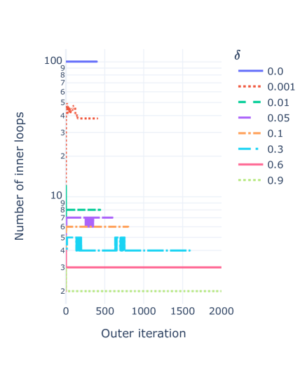
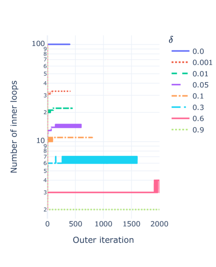
Figure 1: Median plot of the number of inner iterations vs outer iteration index for Frobenius loss (left) and KL loss (right). Various values of the inner stopping criterion parameter $\delta$ are shown in color. The dimensions are $[M,N,R]=[200,100,5]$ and the SNR is $100$. We can observe that increasing the parameters $\delta$ directly influences the number of inner iterations as expected.

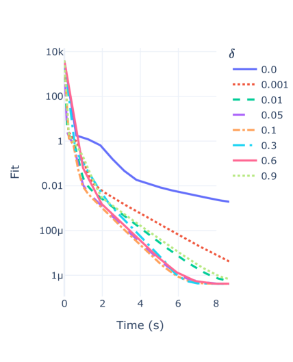
Figure 2: Median plot of normalized cost function values vs time for Frobenius loss (left) and KL loss (right). Various values of the inner stopping criterion parameter $\delta$ are shown in color. Dimensions and SNR are the same as in Figure 1. We can observe a significant speed-up when $\delta$ is above zero, and maximum speed-up around $[0.01,0.1]$.

We may observe that, first, the choice of $\delta$ directly impacts the number of inner iterations on a per-problem basis, which validates that the dynamic inner stopping criterion stops inner iterations adaptively. Second, while there is no clear winner for $\delta$ in the interval $[0.01,0.3]$ and a lot of variabilities, we observe a significant decrease in performance outside that range. Therefore according to these tests, we may set $\delta=0.1$ by default for both losses. Alternatively, we could fix the maximal number of inner iterations to ten iterations since this would lead to a similar performance in this experiment.

5.2 Comparisons with other algorithms

5.2.1 Baseline algorithms

We compare our implementation of the proposed MU algorithm with the following methods:

• Multiplicative Updates (MU) as defined by Lee and Seung [21]. MU is still reported as the state-of-the-art for many problems, in particular when dealing with the KL loss [17]. Thus we use it as a baseline for the proposed fastMU.

• Hierarchical Alternating Least Squares (HALS), which only applies to the Frobenius loss. We used a customized version of the implementation provided in nn-fac [25].

• Nesterov NMF [16] (NeNMF), which is an extension of Nesterov Fast Gradient for computing NMF. We observed that NeNMF provided divergent iterates when used to minimize the KL loss, so it is only used with the Frobenius loss in our experiments.

• Vanilla alternating proximal Gradient Descent (GD) with an aggressive stepsize $1.9/L$ where $L$ is the Lipschitz constant, also only for the Frobenius loss.

To summarize, for the Frobenius loss we evaluate the performance of MU, HALS, NeNMF, and GD against the proposed fastMU algorithm in two variants: fastMU_Fro and the extrapolated fastMU_Fro_ex. For KL, we compare the classical MU algorithm with the proposed fastMU (fastMU_KL) and with the approximate Hessian fastMU_KL_approx. Note that all methods are implemented with the same criterion for stopping inner iterations $\delta=0.1$.

Moreover, in order to further compare the proposed algorithm with the baselines, we also solve the (nonlinear) Nonnegative Least Squares (NLS) problem obtained when factor ${\bf W}$ is known and fixed (to the ground-truth if known). The cost function is then convex and we expect all methods to return the same minimal error. The NLS problem is formally defined as

$$\underset{{\bf H}\in{\mathbb{R}}_{+}^{R\times N}}{\min}~{}\Psi({\bf W},{\bf H})$$ (33)

5.2.2 Comparisons on synthetic dataset

Experiments with the Frobenius loss

Synthetic data are generated with the same procedure as in Section 5.1. All methods start from the same random initialization for each run. Two set of dimensions are used: $[M,N,R]=[1000,400,20]$ and $[M,N,R]=[200,100,5]$. We set the SNR to $100dB$ for the NMF problem, and to $100dB$ or $30dB$ for the NLS problem.

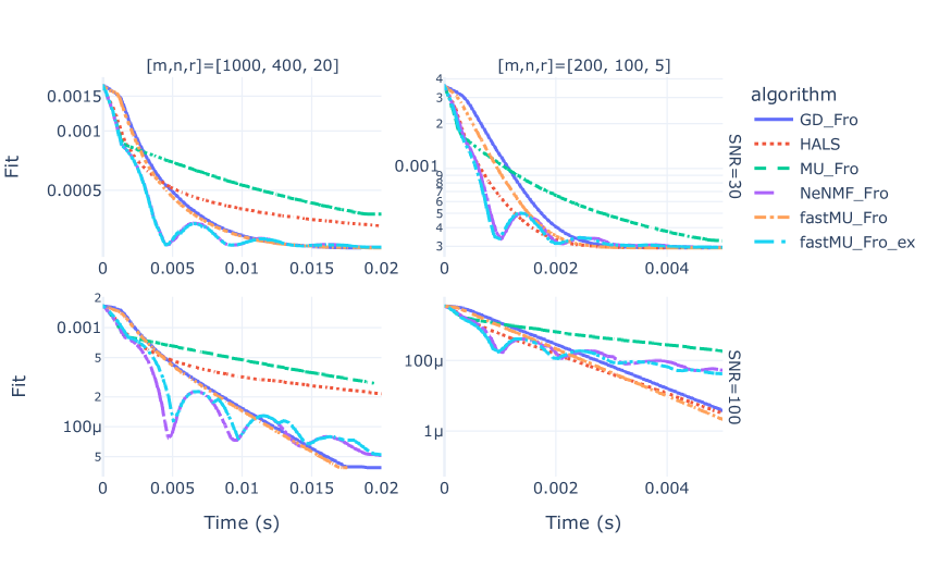
Figure 3: Median plots for the synthetic NLS problem with Frobenius loss. The normalized cost function is plotted against time for various methods. Note that the NeNMF_Fro and fastMU_Fro_ex are almost perfectly overlapping in some of the plots.

Figure 4: Median plots for the synthetic NMF problem with Frobenius loss. The normalized cost function is plotted against time for various methods. The SNR is 100.

Figures 3 and  4 report the results of the Frobenius loss experiments. We may draw several conclusions from these experiments. First, fastMU has competitive performance with the baselines and in particular significantly outperforms MU. In this experiment, fastMU is also faster than HALS for the larger dimensions and rank. Second, the extrapolated algorithms NeNMF and fastMU_Fro_ex are essentially identical in the NLS problem and provide overall the best performing methods for both NMF and NLS problems.

The performance of fastMU is very close to vanilla Gradient Descent in the NLS problem. This may happen if the columns of ${\bf W}$ are close to orthogonality (in which case the Hessian is approximately the identity matrix), but note that the two methods perform differently on the NMF problem where the ground truth ${\bf W}$ is not provided. Gradient descent will perform less favorably on a realistic dataset where factor matrices are correlated, see Section 5.2.3.

Experiments with the KL loss

The data generation is more complex for the KL loss. We overall follow the same procedure as described in Section 5.1. However, because we observed that sparsity has an important impact on MU performance when minimizing the KL loss, we design four different dense or sparse setups:

• setup data sparse: after setting ${\bf V}={\bf W}^{\top}{\bf H}$, the fifty percent smallest entries of ${\bf V}$ are set to zero.

• setup fac sparse: the smallest half of the entries of both ${\bf W}$ and ${\bf H}$ are set to zero.

• setup fac data sparse: we sparsify both the factors and the data with the above procedure.

• setup dense: no sparsification is applied, and the factors and the data are dense.

In all setups, noise is added to the data, after sparsification if it applies, so that $SNR=100$. The dimensions are $[M,N,R]=[200,100,5]$ for the NMF problem, and $[M,N,R]=[2000,1000,40]$ for the NLS problem to test the impact of dimensions on this simpler problem.

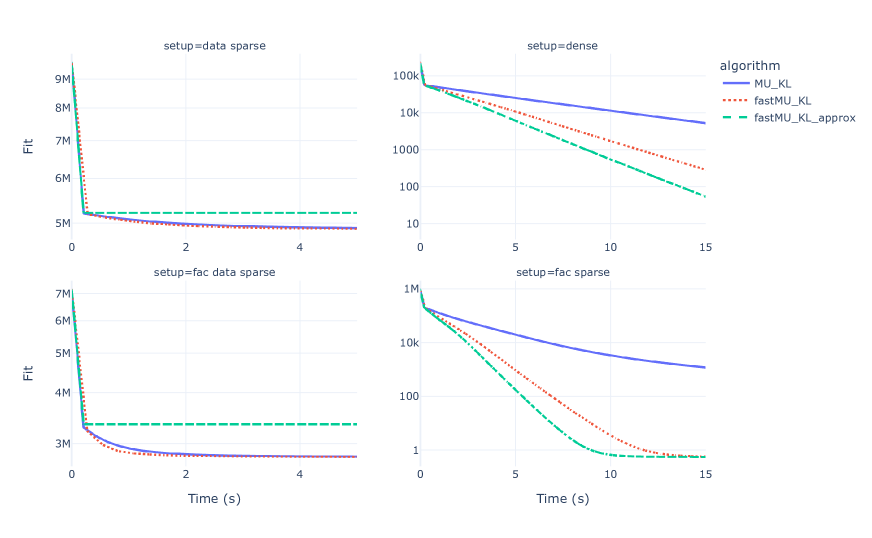
Figure 5: Median plots for the synthetic experiments on the NLS problem with KL loss, showing normalized cost function against time.

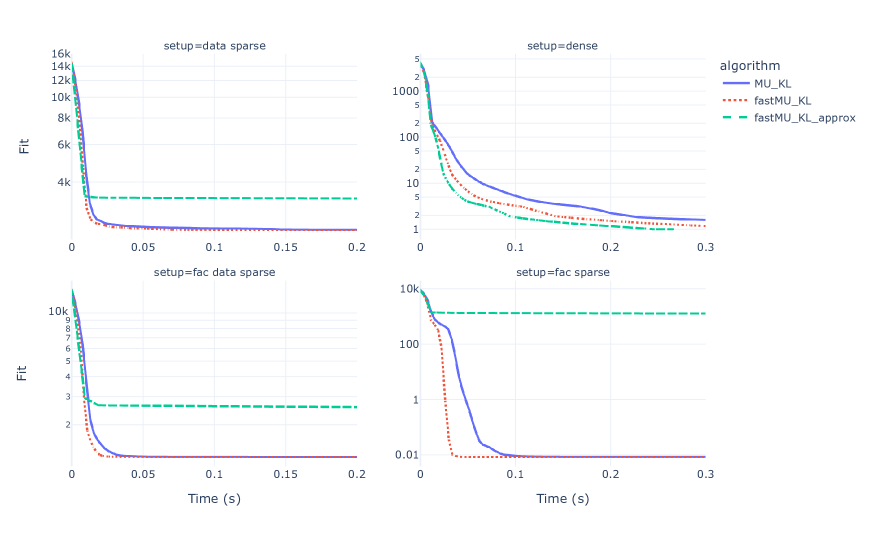
Figure 6: Median plots for the synthetic experiments on the NMF problem with KL loss, showing normalized cost function against time.

Figures 5 and  6 report the KL loss of all compared methods against time for both the NLS and NMF problems in each setup. The most strinking result on these Figures is that fastMU_KL_approx does not converge to a good solution in most of the sparse setup. However, it is the fastest method in the dense setup. Moreover, fastMU_KL converges faster than MU in all the sparse and dense cases for both NLS and NMF problems, and often significantly so. It is nevertheless slower than fastMU_KL_approx in the dense case. The bad convergence behavior of fastMU_KL_approx should rule out its usage unless the data and factors are dense and speed is very critical.

5.2.3 Comparisons on realistic dataset

We used the following dataset to further the comparisons:

• An amplitude spectrogram of dimensions $M=1000$ and $N=1450$ computed from an audio excerpt in the MAPS dataset [12]. More precisely, we hand-picked the file MAPS_MUS_bach-847_AkPnBcht.wav which is a recording of Bach’s second Prelude played on a Yamaha Disklavier. Only the first thirty seconds of the recording are kept, and we also discard all frequencies above 5300Hz. This piece is a moderately difficult piano piece, and NMF has been used in this context to perform blind automatic music transcription, see [3] for more details. Taking inspiration from a model called Attack-Decay [8], in which each rank-one component corresponds to either the attack or the decay of a different key on the piano, we suppose that the amplitude spectrogram is well approximated by an NMF of rank $R=176$, i.e. twice the number of keys on an acoustic piano keyboard.

• An hyperspectral image of dimensions $N=307^{2}$ and $M=162$ called “Urban” which has been used extensively in the blind spectral unmixing literature for showcasing the efficiency of various NMF-based methods, see for instance this survey [4]. Blind spectral unmixing consists in recovering the spectra of the materials present in the image as well as their spatial relative concentrations, and these quantities are in principle estimated as rank-one components in the NMF. It is reported that Urban has between four and six components, we therefore set $R=6$.

In what follows we are not interested in the interpretability of the results since the usefulness of NMF for music automatic transcription and spectral unmixing has already been established in previous works and we do not propose any novelty in the modeling. Instead, we investigate if fastMU and its variants are faster than its competitors to compute NMF on these data.

For both dataset, a reasonable ground-truth for the ${\bf W}$ factor is available, which allows us to also compare algorithms for the NLS problem as well. Indeed in the audio transcription problem, the MAPS database contains individual recordings of each key played on the Disklavier, which we can use to infer ${\bf W}$ as detailed in [35]. In the blind spectral unmixing problem, we use a “fake” ground-truth obtained in [38] where six pixels containing the unmixed spectra have been hand-chosen.

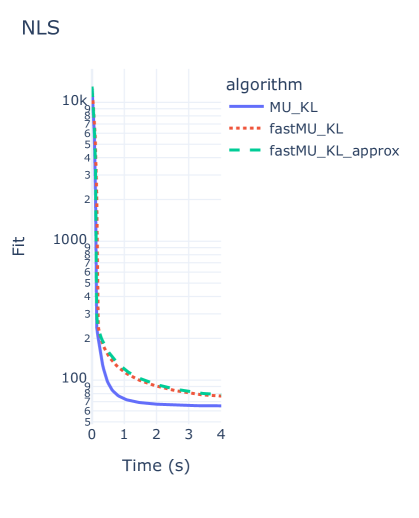
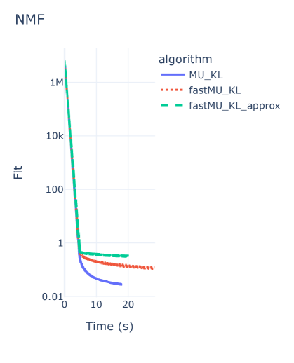
Figure 7: Results of the audio experiment with KL loss. Normalized loss values for five experiments are plotted against time. Left: NLS problem, Right: NMF problem.

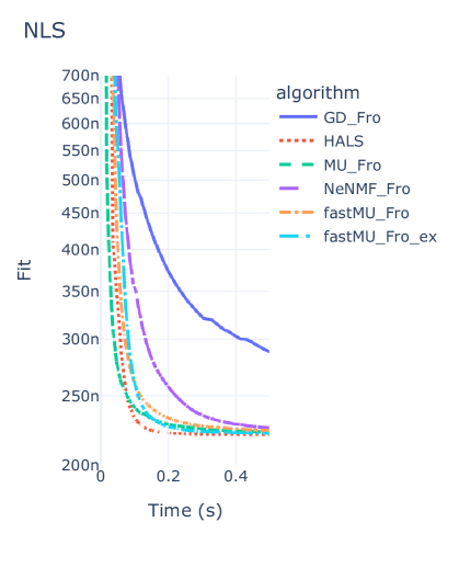
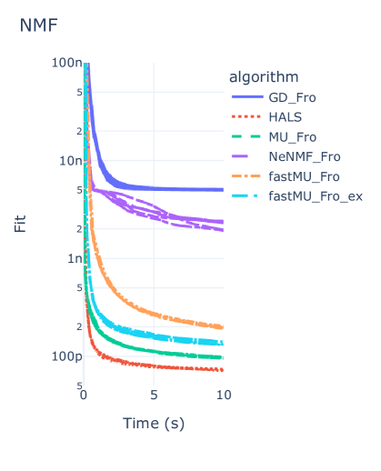
Figure 8: Results of the audio experiment with Frobenius loss. Normalized loss values for ten experiments are plotted against time. Left: NLS problem, Right: NMF problem. Notice the good performance of the vanilla MU algorithm for this dataset.

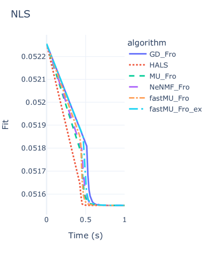
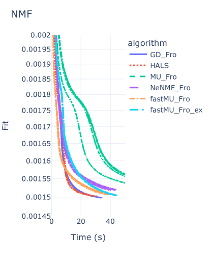
Figure 9: Results of the HSI experiment with Frobenius loss. Normalized loss values for ten experiments are plotted against time. Left: NLS problem, Right: NMF problem.

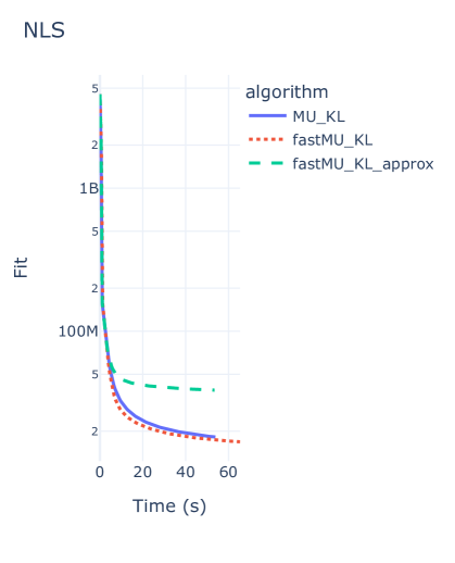
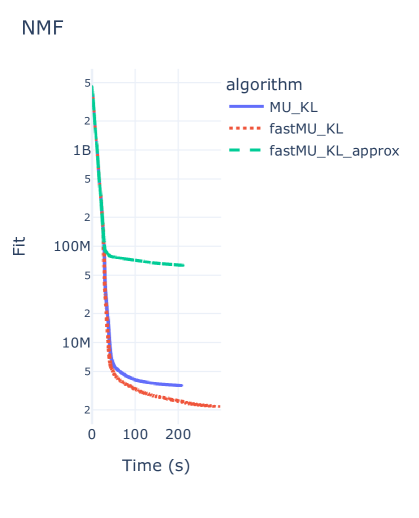
Figure 10: Results of the HSI experiment with KL loss. Normalized loss values for ten experiments are plotted against time. Left: NLS problem, Right: NMF problem.

Figure 7, 8, 9 and 10 respectively show the KL and Frobenius loss function values over time for the power spectrogram and the hyperspectral image. All experiments use $P=5$ different initializations and all the results are superposed on the graphs. Since a reasonable ground truth is available for these problems, we initialized matrix ${\bf W}$ as this ground-truth plus $0.1\eta$ for an i.i.d. uniform noise matrix $\eta$ to stabilize the runs. The NMF HSI (HyperSpectral Image) problem required more outer iterations, the maximum was therefore set to 200.

The results are not entirely consistent with the observations made in the synthetic experiments:

• Frobenius loss: For the audio data, HALS is the best performing method as is generally reported in the literature, followed by MU. When computing NMF, both the fastMU_Fro_ex and fastMU_Fro are close competitors but sadly do not outperform MU. Nevertheless, fastMU improves significantly over MU in the HSI experiment and is competitive with HALS. Moreover, interestingly fastMU_Fro_Ne performs significantly better than NeNMF on both realistic dataset while the two algorithms were performing similarly on the simulated dataset. On the NLS problem results are more ambiguous, but overall fastMU is not a bad competitor to HALS.

• KL loss: we may observe that fastMU is significantly faster than MU in the HSI experiment, but not in the audio experiment. Further research on fastMU seems required to better understand how to further speed-up the method for large dataset, in particular when the rank is large. Furthermore, using the approximate Hessian again proves detrimental to fastMU.

6 Conclusions

In this work, we propose a tighter upper bound of the Hessian matrix to improve the convergence of the MU algorithm for Frobenius and KL loss. The proposed algorithm coined fastMU shows promising performance on both synthetic and real-world data and for both Kullback Leibler and Frobenius loss functions. While, in the experiments we conducted, fastMU is not always better than MU proposed by Lee and Seung, in many cases it is significantly faster. Moreover, it is also competitive with HALS for the Frobenius loss, which is one of the state-of-the-art methods for NMF in that setting. An extrapolated variant of fastMU is investigated which is overall slightly faster than fastMU.

There are many promising research avenues for fastMU. This paper shows how to build a family of majorant functions that contains the Lee and Seung majorant and how to compute a good majorant in that family. However, we do not choose the best majorant in that family as its computation is time consuming. It is anticipated that an efficient algorithmic procedure to compute a better majorant could be designed. One could also search for other majorant families which are even tighter to the original objective, or families of majorants from which sampling is faster. Our attempt at a faster fastMU in the KL loss case did not succeed in the presence of sparse data or factors, but the results on the dense data clearly show potential for further speed-up.

Appendix A Proof of Proposition 1

Proof 3

It is straightforward to prove that a square matrix ${\bf K}$ is a positive semi-definite if and only if ${\bf C}=\operatorname{Diag}({\bf u}){\bf K}\operatorname{Diag}({\bf u})$ is a positive semi-definite matrix for any ${\bf u}\neq 0$. Therefore the proof of this proposition is equivalent to prove that ${\bf C}=\operatorname{Diag}({\bf u})\left(\operatorname{Diag}\left(({\bf B}{\bf u})\oslash{\bf u}\right)-{\bf B}\right)\operatorname{Diag}({\bf u})\$ is positive semi-definite. Indeed, for any ${\bf x}\in{\mathbb{R}}^{N}$ with ${\bf x}\neq 0$ we have

$${\bf x}^{\top}{\bf C}{\bf x} =\sum_{1\leq n\leq N}({\bf B}{\bf u})_{n}u_{n}x_{n}^{2}-\sum_{1\leq n,m\leq N}b_{n,m}u_{n}u_{m}x_{n}x_{m}$$

$$=\sum_{1\leq n,m\leq N}b_{n,m}u_{n}u_{m}x_{n}^{2}-\sum_{1\leq n,m\leq N}b_{n,m}u_{n}u_{m}x_{n}x_{m}$$

$$=\sum_{1\leq n,m\leq N}b_{n,m}u_{n}u_{m}\frac{\left(x_{n}-x_{m}\right)^{2}}{2}\geq 0.$$

This concludes the proof.

References

- [1] Andersen Man Shun Ang and Nicolas Gillis. Accelerating nonnegative matrix factorization algorithms using extrapolation. Neural computation, 31(2):417–439, 2019.
- [2] Amir Beck and Marc Teboulle. A fast iterative shrinkage-thresholding algorithm for linear inverse problems. SIAM Journal on Imaging Sciences, 2(1):183–202, jan 2009.
- [3] Emmanouil Benetos, Simon Dixon, Zhiyao Duan, and Sebastian Ewert. Automatic music transcription: An overview. IEEE Signal Processing Magazine, 36(1):20–30, 2018.
- [4] José M Bioucas-Dias, Antonio Plaza, Nicolas Dobigeon, Mario Parente, Qian Du, Paul Gader, and Jocelyn Chanussot. Hyperspectral unmixing overview: Geometrical, statistical, and sparse regression-based approaches. IEEE journal of selected topics in applied earth observations and remote sensing, 5(2):354–379, 2012.
- [5] J. Bolte, P. L. Combettes, and J.-C. Pesquet. Alternating proximal algorithm for blind image recovery. In 2010 IEEE International Conference on Image Processing. IEEE, sep 2010.
- [6] Jérôme Bolte, Shoham Sabach, and Marc Teboulle. Proximal alternating linearized minimization for nonconvex and nonsmooth problems. Mathematical Programming, 146(1-2):459–494, jul 2013.
- [7] Aleksandar Botev, Guy Lever, and David Barber. Nesterov's accelerated gradient and momentum as approximations to regularised update descent. In 2017 International Joint Conference on Neural Networks (IJCNN). IEEE, may 2017.
- [8] Tian Cheng, Matthias Mauch, Emmanouil Benetos, Simon Dixon, et al. An attack/decay model for piano transcription. In ISMIR 2016 proceedings, 2016.
- [9] Emilie Chouzenoux, Jean-Christophe Pesquet, and Audrey Repetti. A block coordinate variable metric forward-backward algorithm. Journal of Global Optimization, pages 1–29, February 2016.
- [10] Andrzej Cichocki, Rafal Zdunek, and Shun-ichi Amari. Hierarchical als algorithms for nonnegative matrix and 3d tensor factorization. In International Conference on Independent Component Analysis and Signal Separation, pages 169–176. Springer, 2007.
- [11] Jeremy E. Cohen. Shootout. https://github.com/cohenjer/shootout, 2022.
- [12] Valentin Emiya, Nancy Bertin, Bertrand David, and Roland Badeau. Maps-a piano database for multipitch estimation and automatic transcription of music. Research Report, pp.11. inria-00544155, 2010.
- [13] Cédric Févotte and Jérôme Idier. Algorithms for nonnegative matrix factorization with the -divergence. Neural Computation, 23(9):2421–2456, sep 2011.
- [14] Nicolas Gillis. Nonnegative Matrix Factorization. Society for Industrial and Applied Mathematics, Philadelphia, PA, 2020.
- [15] Nicolas Gillis and François Glineur. Accelerated multiplicative updates and hierarchical als algorithms for nonnegative matrix factorization. Neural computation, 24(4):1085–1105, 2012.
- [16] Naiyang Guan, Dacheng Tao, Zhigang Luo, and Bo Yuan. NeNMF: An optimal gradient method for nonnegative matrix factorization. IEEE Transactions on Signal Processing, 60(6):2882–2898, jun 2012.
- [17] Le Thi Khanh Hien and Nicolas Gillis. Algorithms for nonnegative matrix factorization with the kullback–leibler divergence. Journal of Scientific Computing, 87(3):1–32, 2021.
- [18] P.O. Hoyer. Non-negative sparse coding. In Proceedings of the 12th IEEE Workshop on Neural Networks for Signal Processing. IEEE.
- [19] David R. Hunter and Kenneth Lange. [optimization transfer using surrogate objective functions]: Rejoinder. Journal of Computational and Graphical Statistics, 9(1):52, mar 2000.
- [20] David R. Hunter and Kenneth Lange. A tutorial on mm algorithms. American Statistician, 58(1):30–37, February 2004.
- [21] Daniel D. Lee and H. Sebastian Seung. Learning the parts of objects by non-negative matrix factorization. Nature, 1999.
- [22] Daniel D. Lee and H. Sebastian Seung. Algorithms for non-negative matrix factorization. In Advances in Neural Information Processing Systems. MIT Press, 2001.
- [23] Valentin Leplat, Nicolas Gillis, and Jérôme Idier. Multiplicative updates for nmf with -divergences under disjoint equality constraints. SIAM Journal on Matrix Analysis and Applications, 42(2):730–752, 2021.
- [24] Z. Q. Luo and P. Tseng. On the convergence of the coordinate descent method for convex differentiable minimization. Journal of Optimization Theory and Applications, 72(1):7–35, jan 1992.
- [25] Axel Marmoret and Jérémy Cohen. nn_fac: Nonnegative factorization techniques toolbox, 2020.
- [26] Brendan O’Donoghue and Emmanuel Candès. Adaptive restart for accelerated gradient schemes. Foundations of Computational Mathematics, 15(3):715–732, jul 2013.
- [27] Pentti Paatero and Unto Tapper. Positive matrix factorization: A non-negative factor model with optimal utilization of error estimates of data values. Environmetrics, 5(2):111–126, jun 1994.
- [28] Audrey Repetti, Mai Quyen Pham, Laurent Duval, Emilie Chouzenoux, and Jean-Christophe Pesquet. Euclid in a taxicab: Sparse blind deconvolution with smoothed regularization. IEEE Signal Processing Letters, 22(5):539–543, may 2015.
- [29] Romain Serizel, Slim Essid, and Gaël Richard. Mini-batch stochastic approaches for accelerated multiplicative updates in nonnegative matrix factorisation with beta-divergence. In 2016 IEEE 26th International Workshop on Machine Learning for Signal Processing (MLSP), pages 1–6. IEEE, 2016.
- [30] Yong Sheng Soh and Antonios Varvitsiotis. A non-commutative extension of lee-seung's algorithm for positive semidefinite factorizations. In M. Ranzato, A. Beygelzimer, Y. Dauphin, P.S. Liang, and J. Wortman Vaughan, editors, Advances in Neural Information Processing Systems, volume 34, pages 27491–27502. Curran Associates, Inc., 2021.
- [31] N. Takahashi, J. Katayama, and J. Takeuchi. A generalized sufficient condition for global convergence of modified multiplicative updates for nmf. In Int. Symp. Nonlinear Theory Appl., 2014.
- [32] Norikazu Takahashi and Ryota Hibi. Global convergence of modified multiplicative updates for nonnegative matrix factorization. Computational Optimization and Applications, 57(2):417–440, aug 2013.
- [33] Norikazu Takahashi and Masato Seki. Multiplicative update for a class of constrained optimization problems related to nmf and its global convergence. In 2016 24th European Signal Processing Conference (Eusipco), pages 438–442. IEEE, 2016.
- [34] Leo Taslaman and Björn Nilsson. A framework for regularized non-negative matrix factorization, with application to the analysis of gene expression data. PLoS ONE, 7(11):e46331, nov 2012.
- [35] Haoran Wu, Axel Marmoret, and Jeremy E. Cohen. Semi-supervised convolutive NMF for automatic piano transcription. In Sound and Music Computing 2022. Zenodo, june 2022.
- [36] Yangyang Xu and Wotao Yin. A block coordinate descent method for regularized multiconvex optimization with applications to nonnegative tensor factorization and completion. SIAM Journal on Imaging Sciences, 6(3):1758–1789, jan 2013.
- [37] Renbo Zhao and Vincent YF Tan. A unified convergence analysis of the multiplicative update algorithm for nonnegative matrix factorization. In 2017 IEEE International Conference on Acoustics, Speech and Signal Processing (ICASSP), pages 2562–2566. IEEE, 2017.
- [38] Feiyun Zhu. Hyperspectral unmixing: ground truth labeling, datasets, benchmark performances and survey. arXiv preprint arXiv:1708.05125, 2017.