Adaptive stabilized finite elements via residual minimization onto bubble enrichments

Jose G. Hasbani jose.hasbani@vistaenergy.com Paulina Sepúlveda Ignacio Muga Victor M. Calo Sergio Rojas Vista Energy, Argentina Instituto de Matemáticas, Pontificia Universidad Católica de Valparaíso, Valparaíso, Chile School of Electrical Engineering, Computing and Mathematical Sciences, Curtin University, Bentley, Australia
Abstract

The Adaptive Stabilized Finite Element method (AS-FEM) developed in [16] combines the idea of the residual minimization method with the inf-sup stability offered by the discontinuous Galerkin (dG) frameworks. As a result, the discretizations deliver stabilized approximations and residual representatives in the dG space that can drive automatic adaptivity. We generalize AS-FEM by considering continuous test spaces; thus, we propose a residual minimization method on a stable Continuous Interior Penalty (CIP) formulation that considers a C0superscript𝐶0C^{0}-conforming trial FEM space and a test space based on the enrichment of the trial space by bubble functions. In our numerical experiments, the test space choice results in a significant reduction of the total degrees of freedom compared to the dG test spaces of [16] that converge at the same rate. Moreover, as trial and test spaces are C0superscript𝐶0C^{0}-conforming, implementing a full dG data structure is unnecessary, simplifying the method’s implementation considerably and making it appealing for industrial applications, see [42].

keywords:
adaptivity, stabilized finite elements , residual minimization, Continuous Galerkin , Continuous Interior Penalty
journal: CAMWA

1 Introduction

The continuous Galerkin (cG) finite element methods (FEM) for advection-dominated reaction-type problems might suffer from instabilities. When the hyperbolic character of the problem becomes predominant, interior and outflow layers form, causing large local gradients in the solution. The cG-FEM is unstable in this regime, and various stabilized methods have been proposed. Techniques in the framework of cG-FEM are available in the literature, including Streamline-Upwind Petrov-Galerkin (SUPG) method [39], residual-free bubbles [8], and subviscosity models for advection-diffusion problems [35]. The relationships between the aforementioned strategies are also well understood in almost all cases. For example, in [7], a relation between stabilized finite element methods and the Galerkin method employing bubble functions was established for the advection-diffusion problems. In that work, the authors showed that bubble functions help stabilize the advective operator without using upwinding or any other numerical strategy. In particular, for the advection-diffusion problem, the Galerkin method employing piecewise linear functions enriched with bubble functions was shown to be equivalent to the SUPG method in the diffusive limit. Applications of this type of enrichment include stabilization of Stokes flow [3] and stabilization of Galerkin approximation using artificial viscosity [35]. Hughes generalized the stabilized methods construction into a unified framework in the variational multiscale framework [36, 37]; these ideas were extended to other applications such as turbulence modeling [38, 6]. Although those strategies are now reaching maturity, those methods have some drawbacks in certain complex flow regimes. For instance, the SUPG stabilization becomes non-symmetric and does not allow lumped mass, the residual free bubbles method adds additional degrees of freedom to the system, and the projection methods introduce hierarchical meshes for the projection on the subgrid viscosity model [35].

Interior Penalty penalty methods using continuous functions were introduced originally by [4, 29] for different problems, namely, the biharmonic operator and the second-order elliptic and parabolic problems. These methods penalize the flux jump of the discrete solution at mesh interfaces. Thus, the method [29] keeps the benefits of continuous finite element methods as they were standard for elliptic problems while simultaneously managing the difficulties encountered by these methods when the hyperbolic character of diffusion-advection problems becomes dominant in the advection limit. However, the robustness of the error estimate in the advection-dominated regime was not analyzed until [13], in which the analysis was based on linear finite elements. Recently, a generalized hp-convergence analysis for a high-order Continuous Interior Penalty (CIP) finite element method was presented in [12] applied to advection-reaction and diffusion-advection-reaction problems.

Alternatively, the Continuous Interior Penalty (CIP) method, introduced in [30], for advection-diffusion-reaction problems; this method adds an L2superscript𝐿2L^{2} penalization to the flux jumps (i.e., gradient jumps for uniform coefficients) over the mesh interior edges/facets to stabilize a continuous approximation (see [13, 11, 14, 12]). In [11] and [12], the authors developed a hp-convergence analysis for high-order CIP methods for advection-reaction and advection-diffusion problems. This stabilization does not depend on the diffusion coefficient and considers the case of pure advection. Moreover, Burman [10] introduced a formulation relating the stabilized continuous and discontinuous Galerkin frameworks with the CIP formulation. In that work, the author showed that both frameworks can be condensed into a single formulation, presented a robust a-posteriori error estimate for advection-reaction problems to guide adaptivity, and compared the low-order CIP and dG approximations using an adaptive approach showing that the CIP method achieves optimal convergence in the L2superscript𝐿2L^{2} norm.

More recently, the Adaptive Stabilized Finite Element Method (AS-FEM) was introduced (see [16]). This method formulates residual minimization problems within a dG mathematical framework. Namely, a discrete approximation of the solution in a continuous trial space is constructed by minimizing the residual in the dual norm of a dG test space with inf-sup stability. The residual minimization problem is equivalent to a saddle-point problem that inherits dG’s inf-sup stability. There are some similarities with the Discontinuous Petrov-Galerkin (DPG) method as both minimize the residual in a non-standard norm (see, e.g., [18, 15, 23, 26, 24, 25, 45, 46, 47, 50]). However, AS-FEM builds on non-conforming dG formulations, where stronger norms than those used in DPG may be chosen when the test space contains continuous functions. Application examples include diffusive-advective-reactive problems [20], incompressible Stokes flows [41, 43], continuation analysis of compaction banding in geomaterials [19] and weak constraint enforcement for advection-dominated diffusion problems [21]. The method has been successfully applied to several nonlinear problems, such as dynamic fracture propagation [42], mineral deposition [48], and the method of lines for Bratu’s equation [33]. In [49], the authors extend AS-FEM to goal-oriented adaptivity (GoA); they describe a general theory for problems with well-posed formulations and provide error estimates to guide the GoA for advection-diffusion-reaction problems. In addition, they define a discrete adjoint system as a saddle-point problem where the discontinuous conforming space across element interfaces restricts the solution. The same dG inf-sup arguments guarantee the well-posedness of this adjoint saddle-point problem. Solving the primal and the adjoint problem requires the solution of a single saddle-point problem with two right-hand sides. Moreover, the authors proposed two alternative stable discrete problems that can measure the discrete adjoint error of the problem; a strategy similar to a recent DPG theory [40] in which the adjoint problem is solved using the original saddle-point formulation with a different right-hand side.

The method proposed in [16] and its extension to GoA in [49] contain a general theory motivated in a dG framework; this framework can also use continuous test spaces (see [42] for a demonstration of this idea). Herein, we analyze the extension of the AS-FEM based on a stable CIP formulation for an advection-reaction problem proposed in [13, 12]. We consider a bubble-enriched continuous trial space as a test space to explode the power of the residual minimization method, which delivers an error representative which is robust and reliable to guide adaptive mesh refinements. This space is sufficient to guarantee a distance to the trial space and obtain a residual representative to drive adaptivity.

We test the method’s performance in a challenging advection-reaction problem. We choose this model problem since the elliptic character of the diffusion term in the advection-diffusion equation has some smoothing properties on the transport problem. Nonetheless, extending the results obtained in this work to advection-diffusion-reaction problems is straightforward. Additionally, we present a new result on a priori error estimates for the residual minimization method using continuous test spaces, which relies on an orthogonality argument for boundedness of the discrete bilinear form and coercivity that proves quasi-optimal convergence for advection-dominated problems. Finally, we perform adaptive numerical experiments using energy-based and GoA strategies [16, 49]. In the energy-based examples, we evaluate the performance of the residual error estimate obtained by the residual minimization method against the a-posteriori error estimate of [10] regarding the relative error in the L2superscript𝐿2L^{2}-norm and the resulting adapted meshes.

The remainder of this paper is structured as follows: Section 2 introduces the advection-reaction model problem. In Section 3, the notation and the discrete problem settings are presented. In Section 4, we describe the CIP formulation in the context of bubble-enriched continuous spaces, its main properties, and the residual minimization method, and we state the main result of this work. In Section 5, we present numerical experiments to show the method’s performance and compare the results with other methods found in the literature. Finally, Section 6 summarizes the main contributions of this work and points to possible future research directions.

2 Model problem.

Let ΩdΩsuperscript𝑑\Omega\subset\mathbb{R}^{d} ( d=2,3𝑑23d=2,3) be an open bounded connected set, with Lipschitz boundary ΩΩ\partial\Omega, and outward normal vector n. Consider an advection field b[L(Ω)]dbsuperscriptdelimited-[]superscript𝐿Ω𝑑\textbf{b}\in[L^{\infty}(\Omega)]^{d} such that bL(Ω)bsuperscript𝐿Ω\nabla\cdot\textbf{b}\in L^{\infty}(\Omega), and a reaction coefficient μL(Ω)𝜇superscript𝐿Ω\mu\in L^{\infty}(\Omega). Let us define the following graph space:

W:={wL2(Ω):bwL2(Ω)},assign𝑊conditional-set𝑤superscript𝐿2Ωb𝑤superscript𝐿2Ω\displaystyle W:=\left\{w\in L^{2}(\Omega):\,\textbf{b}\cdot\nabla w\in L^{2}(\Omega)\right\}, (1)

equipped with the graph norm wW2=wL2(Ω)2+bwL2(Ω)2superscriptsubscriptnorm𝑤𝑊2superscriptsubscriptnorm𝑤superscript𝐿2Ω2superscriptsubscriptnormb𝑤superscript𝐿2Ω2\|w\|_{W}^{2}=\|w\|_{L^{2}(\Omega)}^{2}+\|\textbf{b}\cdot\nabla w\|_{L^{2}(\Omega)}^{2}. The advection field b partitions the boundary ΩΩ\partial\Omega into inflow, characteristic, and outflow parts, having the following expressions when b is continuous111These boundaries may also be defined for the general case b[L(Ω)]dbsuperscriptdelimited-[]superscript𝐿Ω𝑑\textbf{b}\in[L^{\infty}(\Omega)]^{d} and bL(Ω)bsuperscript𝐿Ω\nabla\cdot\textbf{b}\in L^{\infty}(\Omega); see [9, Section 2].:

ΩsubscriptΩ\displaystyle\partial\Omega_{-} :={xΩ:b(x)n(x)<0},assignabsentconditional-set𝑥Ωb𝑥n𝑥0\displaystyle:=\{x\in\partial\Omega:\textbf{b}(x)\cdot\textbf{n}(x)<0\}, (2a)
Ω0subscriptΩ0\displaystyle\partial\Omega_{0} :={xΩ:b(x)n(x)=0},assignabsentconditional-set𝑥Ωb𝑥n𝑥0\displaystyle:=\{x\in\partial\Omega:\textbf{b}(x)\cdot\textbf{n}(x)=0\}, (2b)
Ω+subscriptΩ\displaystyle\partial\Omega_{+} :={xΩ:b(x)n(x)>0}.assignabsentconditional-set𝑥Ωb𝑥n𝑥0\displaystyle:=\{x\in\partial\Omega:\textbf{b}(x)\cdot\textbf{n}(x)>0\}. (2c)

Given fL2(Ω)𝑓superscript𝐿2Ωf\in L^{2}(\Omega), we consider the advection-reaction model problem that seeks uW𝑢𝑊u\in W such that:

{bu+μu=f, in Ωu=0, on Ω.casesb𝑢𝜇𝑢𝑓 in Ω𝑢0 on subscriptΩ\displaystyle\left\{\begin{array}[]{l}\begin{array}[]{rl}\textbf{b}\cdot\nabla u+\mu\,u=f,&\text{ in }\Omega\vskip 3.0pt plus 1.0pt minus 1.0pt\\ u=0,&\text{ on }\partial\Omega_{-}.\end{array}\end{array}\right. (6)

We point out that traces of W𝑊W are well-defined222See, e.g., [27, Section 2.1.3] and [34] for an extension., implying that the linear space W0,:={wW:w|Ω=0}assignsubscript𝑊0conditional-set𝑤𝑊evaluated-at𝑤subscriptΩ0W_{0,-}:=\{w\in W:w|_{\partial\Omega_{-}}=0\} is also well-defined. Moreover, equation (6) translates into finding uW0,𝑢subscript𝑊0u\in W_{0,-} such that Au=f𝐴𝑢𝑓Au=f, where A:W0,L2(Ω):𝐴subscript𝑊0superscript𝐿2ΩA:W_{0,-}\to L^{2}(\Omega) (defined as Aw:=bw+μwassign𝐴𝑤b𝑤𝜇𝑤A\,w:=\textbf{b}\cdot\nabla w+\mu w, for all wW0,𝑤subscript𝑊0w\in W_{0,-}) is a linear isomorphism provided

μ12bμ0>0, a.e. in Ω,formulae-sequence𝜇12bsubscript𝜇00 a.e. in Ω\mu-\dfrac{1}{2}\nabla\cdot\textbf{b}\geq\mu_{0}>0,\quad\text{ {a.e.} in }\Omega, (7)

holds for some positive constant μ0subscript𝜇0\mu_{0} (see [31, Proposition 5.9] ). When μ=0𝜇0\mu=0 and b=0b0\nabla\cdot\textbf{b}=0, then A𝐴A still is a linear isomorphism provided that b is an ΩΩ\Omega-filling field (see [31, Remark 5.10]).

Remark 1 (Non-homogeneous inflow boundary condition).

The trace operator is linear, continuous, and surjective from W𝑊W onto the space

L2(|bn|;Ω):={w measurable in Ω:Ω|bn|w2<+},assignsuperscript𝐿2bnΩconditional-set𝑤 measurable in ΩsubscriptΩbnsuperscript𝑤2L^{2}(|\textbf{b}\cdot\textbf{n}|;\partial\Omega):=\left\{w\text{ measurable in }\partial\Omega:\int_{\partial\Omega}|\textbf{b}\cdot\textbf{n}|w^{2}<+\infty\right\},

which allows us to consider non-homogeneous inflow boundary conditions in (6), whenever the inflow data belongs to L2(|bn|;Ω)superscript𝐿2bnΩL^{2}(|\textbf{b}\cdot\textbf{n}|;\partial\Omega) (see, e.g., [27, Lemma 2.11]).

3 Notation, discrete spaces and interpolation results.

Let ΩhsubscriptΩ\Omega_{h} be a quasi-uniform simplicial mesh of ΩΩ\Omega, defined as a collection of finite many open connected elements TΩ𝑇ΩT\subset\Omega with Lipschitz boundaries, such that Ω¯¯Ω\overline{\Omega} is the union of the closures of all mesh elements T𝑇{T} in ΩΩ\Omega. We denote by h0subscriptsuperscript0\mathcal{F}^{0}_{h} the collection of all interior element boundaries (edges/faces); by hsubscriptsuperscript\mathcal{F}^{\partial}_{h} the collection of those element boundaries that belong to ΩΩ\partial\Omega; and set h:=h0hassignsubscriptsubscriptsuperscript0subscriptsuperscript\mathcal{F}_{h}:=\mathcal{F}^{0}_{h}\bigcup\mathcal{F}^{\partial}_{h}. Given TΩh𝑇subscriptΩT\in\Omega_{h}, let us denote the diameter of T𝑇T by hT>0subscript𝑇0h_{T}>0, and let h:=maxTΩhhTassign𝑇subscriptΩsubscript𝑇h:=\underset{T\in\Omega_{h}}{\max}\,h_{T}. Analogously, for eh0𝑒subscriptsuperscript0e\subset\mathcal{F}^{0}_{h}, let he>0subscript𝑒0h_{e}>0 be the diameter e𝑒e.

For a given set Dd𝐷superscript𝑑D\subset\mathbb{R}^{d}, consider the Sobolev space Hs(D)superscript𝐻𝑠𝐷H^{s}(D) of order s0𝑠0s\geq 0, and denote by s,D\|\cdot\|_{s,D} its well-known norm (see, e.g., [1]). By convention, set L2(D)=H0(D)superscript𝐿2𝐷superscript𝐻0𝐷L^{2}(D)=H^{0}(D) and abbreviate the L2(D)superscript𝐿2𝐷L^{2}(D) inner product by (,)Dsubscript𝐷(\cdot,\cdot)_{D} and its respective norm by D\|\cdot\|_{D}.

nesubscriptn𝑒\textbf{n}_{e}e𝑒eT+superscript𝑇T^{+}Tsuperscript𝑇T^{-}
Figure 1: Notation for an interface

We define the broken Sobolev space Hs(Ωh)superscript𝐻𝑠subscriptΩH^{s}(\Omega_{h}) as follows

Hs(Ωh):={vL2(Ω):v|THs(T) for all TΩh},assignsuperscript𝐻𝑠subscriptΩconditional-set𝑣superscript𝐿2Ωevaluated-at𝑣𝑇superscript𝐻𝑠𝑇 for all 𝑇subscriptΩH^{s}(\Omega_{h}):=\{v\in L^{2}(\Omega):v|_{T}\in H^{s}(T)\text{ for all }T\in\Omega_{h}\},

with its corresponding broken norm s,Ωh2:=TΩh()|Ts,T2\|\cdot\|_{s,\Omega_{h}}^{2}:=\displaystyle\sum_{T\in\Omega_{h}}\|(\,\cdot\,)|_{T}\|^{2}_{s,T}\,. When s>12𝑠12s>\frac{1}{2}, traces over the edges of elements are well-defined. Thus, for eh0𝑒subscriptsuperscript0e\subset\mathcal{F}^{0}_{h}, we define the jump of a function vHs(Ωh)𝑣superscript𝐻𝑠subscriptΩv\in H^{s}(\Omega_{h}) across e𝑒e, as the following expression:

\llbracketv\rrbracket|e:=v|T+v|T,eh0,formulae-sequenceassignevaluated-at\llbracket𝑣\rrbracket𝑒evaluated-at𝑣superscript𝑇evaluated-at𝑣superscript𝑇for-all𝑒subscriptsuperscript0\llbracket v\rrbracket\big{|}_{e}:=v\big{|}_{T^{+}}-v\big{|}_{T^{-}},\qquad\forall e\in\mathcal{F}^{0}_{h}\,, (8)

where v|T+evaluated-at𝑣superscript𝑇v\big{|}_{T^{+}} and v|Tevaluated-at𝑣superscript𝑇v\big{|}_{T^{-}} are the traces over e𝑒e related with a predefined normal nesubscriptn𝑒\textbf{n}_{e} (see Figure 1 for a reference of the interface notation).

3.1 Discrete spaces

Let p(T)superscript𝑝𝑇\mathbb{P}^{p}(T) be the space of polynomials of total degree pabsent𝑝\leq p over T𝑇T. We consider the following discrete spaces:

Uhp:={vC0(Ω):v|Tp(T),TΩh},assignsubscriptsuperscript𝑈𝑝conditional-set𝑣superscript𝐶0Ωformulae-sequenceevaluated-at𝑣𝑇superscript𝑝𝑇for-all𝑇subscriptΩU^{p}_{h}:=\left\{v\in C^{0}(\Omega):v|_{T}\in\mathbb{P}^{p}(T),\,\forall T\in\Omega_{h}\right\}, (9)
Vhp:={vL2(Ω):v|Tp(T),TΩh},assignsuperscriptsubscript𝑉𝑝conditional-set𝑣superscript𝐿2Ωformulae-sequenceevaluated-at𝑣𝑇superscript𝑝𝑇for-all𝑇subscriptΩV_{h}^{p}:=\left\{v\in L^{2}(\Omega):v|_{T}\in\mathbb{P}^{p}(T),\,\forall T\in\Omega_{h}\right\}, (10)

and define the space of local bubble functions of degree kabsent𝑘\leq k, with k>d𝑘𝑑k>d (see [3]), by

𝔹k(Ωh):={vH01(Ω):v|Tk(T)H01(T),TΩh}.assignsuperscript𝔹𝑘subscriptΩconditional-set𝑣superscriptsubscript𝐻01Ωformulae-sequenceevaluated-at𝑣𝑇superscript𝑘𝑇subscriptsuperscript𝐻10𝑇for-all𝑇subscriptΩ\mathbb{B}^{k}(\Omega_{h}):=\left\{v\in H_{0}^{1}(\Omega):\,v|_{T}\in\mathbb{P}^{k}(T)\bigcap H^{1}_{0}(T),\,\forall T\in\Omega_{h}\right\}. (11)

Finally, we define the bubble-enriched continuous function space, with k>max{p,d}𝑘𝑝𝑑k>\max\{p,d\}, as

Uhp,k:=Uhp+𝔹k(Ωh).assignsubscriptsuperscript𝑈𝑝𝑘subscriptsuperscript𝑈𝑝superscript𝔹𝑘subscriptΩU^{p,k}_{h}:=U^{p}_{h}+\mathbb{B}^{k}(\Omega_{h}). (12)

As an example, in the case of triangular elements and k=3𝑘3k=3, a local bubble function over T𝑇T can be defined as a cubic function spanned by λ1λ2λ3subscript𝜆1subscript𝜆2subscript𝜆3\lambda_{1}\lambda_{2}\lambda_{3}, where λ1,λ2,λ3subscript𝜆1subscript𝜆2subscript𝜆3\lambda_{1},\lambda_{2},\lambda_{3} are the barycentric coordinates on T𝑇T, see [3, 44, 42].

Remark 2 (Containment of discrete spaces).

When kp𝑘𝑝k\leq p implies Uhp,kUhpsubscriptsuperscript𝑈𝑝𝑘subscriptsuperscript𝑈𝑝U^{p,k}_{h}\equiv U^{p}_{h}; alternatively, when k>p𝑘𝑝k>p, the following discrete space contention occurs

UhpUhp,kUhk.superscriptsubscript𝑈𝑝superscriptsubscript𝑈𝑝𝑘superscriptsubscript𝑈𝑘U_{h}^{p}\subset U_{h}^{p,k}\subseteq U_{h}^{k}. (13)

3.2 Interpolation results

Our convergence analysis follows [12] for the hp𝑝hp-continuous interior penalty (CIP) method, which uses trace and inverse-trace inequalities, local interpolation results, and error estimates for the L2(Ω)superscript𝐿2ΩL^{2}(\Omega)-projection. Here is a summary of these results in two dimensions (i.e., d=2𝑑2d=2). We simplify notation by abbreviating the inequalities aCb𝑎𝐶𝑏a\leq C\,b as abless-than-or-similar-to𝑎𝑏a\lesssim b whenever the positive constant C𝐶C is independent of the mesh and polynomial degree.

Definition 1 (Admissible set).

Given a simplex T𝑇T, let np:=dimp(T)assignsubscript𝑛𝑝dimensionsuperscript𝑝𝑇n_{p}:=\dim\mathbb{P}^{p}(T). A nonempty set of nodes 𝒜={ai}1inp𝒜subscriptsubscript𝑎𝑖1𝑖subscript𝑛𝑝\mathcal{A}=\{a_{i}\}_{1\leq i\leq n_{p}} of T𝑇T is admissible if and only if 𝒜𝒜\mathcal{A} is unisolvent in p(T)superscript𝑝𝑇\mathbb{P}^{p}(T) and 𝒜e𝒜𝑒\mathcal{A}\cap e is unisolvent in p(e)superscript𝑝𝑒\mathbb{P}^{p}(e), for all edges eT𝑒𝑇e\subset\partial T.

Given a unisolvent set of nodes 𝒜𝒜\mathcal{A} of a simplex T𝑇T, define:

𝒜p(T):={vp(T):v(ai)=0,ai𝒜T}.assignsubscriptsuperscript𝑝𝒜𝑇conditional-set𝑣superscript𝑝𝑇formulae-sequence𝑣subscript𝑎𝑖0for-allsubscript𝑎𝑖𝒜𝑇\mathbb{P}^{p}_{\mathcal{A}}(T):=\left\{v\in\mathbb{P}^{p}(T):v(a_{i})=0,\forall a_{i}\in\mathcal{A}\setminus\partial T\right\}.
Assumption 1.

Let T^^𝑇\hat{T} be the reference element; for p(T^)superscript𝑝^𝑇\mathbb{P}^{p}(\hat{T}), there exists an admissible set of nodes 𝒜^^𝒜\hat{\mathcal{A}} of T^^𝑇\hat{T}, such that

vT^p1/2vT^,v𝒜^p(T^).formulae-sequenceless-than-or-similar-tosubscriptnorm𝑣^𝑇superscript𝑝12subscriptnorm𝑣^𝑇for-all𝑣superscriptsubscript^𝒜𝑝^𝑇\displaystyle\|v\|_{\hat{T}}\lesssim p^{-1/2}\|v\|_{\partial\hat{T}}\,,\qquad\forall v\in\mathbb{P}_{\hat{\mathcal{A}}}^{p}(\hat{T}).

In [12, Section 5.1], the authors establish that Assumption 1 leads to the following inequalities.

Lemma 1 (Trace and inverse trace inequalities on triangles).

Under Assumption 1, the following inequalities hold for any TΩh𝑇subscriptΩT\in\Omega_{h}:

vT(p2hT)12vT,vp(T);formulae-sequenceless-than-or-similar-tosubscriptnorm𝑣𝑇superscriptsuperscript𝑝2subscript𝑇12subscriptnorm𝑣𝑇for-all𝑣superscript𝑝𝑇{\left|\kern-1.07639pt\left|v\right|\kern-1.07639pt\right|}_{\partial T}\lesssim\left(\dfrac{p^{2}}{h_{T}}\right)^{\frac{1}{2}}{\left|\kern-1.07639pt\left|v\right|\kern-1.07639pt\right|}_{T},\quad\forall v\in\mathbb{P}^{p}(T); (14)
vT(hTp)12vT,vp,0(T),formulae-sequenceless-than-or-similar-tosubscriptnorm𝑣𝑇superscriptsubscript𝑇𝑝12subscriptnorm𝑣𝑇for-all𝑣superscript𝑝0𝑇{\left|\kern-1.07639pt\left|v\right|\kern-1.07639pt\right|}_{T}\lesssim\left(\dfrac{h_{T}}{p}\right)^{\frac{1}{2}}{\left|\kern-1.07639pt\left|v\right|\kern-1.07639pt\right|}_{\partial T},\quad\forall v\in\mathbb{P}^{p,0}(T), (15)

where p,0(T)superscript𝑝0𝑇\mathbb{P}^{p,0}(T) denotes the subspace of p(T)superscript𝑝𝑇\mathbb{P}^{p}(T) spanned by those polynomials vanishing at all interior nodes of T𝑇T.

Definition 2 (Oswald Interpolation).

Given TΩh𝑇subscriptΩT\in\Omega_{h}, let 𝒜Tsubscript𝒜𝑇\mathcal{A}_{T} be the image of the admissible set 𝒜^^𝒜\hat{\mathcal{A}} (see Assumption 1) under an affine transformation mapping from T^^𝑇\hat{T} onto T𝑇T. For each node a𝒜T𝑎subscript𝒜𝑇a\in\mathcal{A}_{T}, consider the patch of elements Ωa:={TΩh,aT¯}assignsubscriptΩ𝑎formulae-sequence𝑇subscriptΩ𝑎¯𝑇\Omega_{a}:=\big{\{}T\in\Omega_{h},a\in\overline{T}\big{\}}. The Oswald interpolation operator IOs:VhpUhp:subscript𝐼𝑂𝑠superscriptsubscript𝑉𝑝superscriptsubscript𝑈𝑝I_{Os}:V_{h}^{p}\to U_{h}^{p} (see, e.g., [12, Section 5.5.2]), is defined locally by setting

IOs(vh)(a):=1|Ωa|TΩavh|T(a),vhVhp,formulae-sequenceassignsubscript𝐼𝑂𝑠subscript𝑣𝑎evaluated-at1subscriptΩ𝑎subscript𝑇subscriptΩ𝑎subscript𝑣𝑇𝑎for-allsubscript𝑣superscriptsubscript𝑉𝑝I_{Os}(v_{h})(a):=\dfrac{1}{|\Omega_{a}|}\sum_{T\in\Omega_{a}}v_{h}\big{|}_{T}(a)\,,\qquad\forall v_{h}\in V_{h}^{p}, (16)

where |Ωa|subscriptΩ𝑎|\Omega_{a}| stands for the cardinality of ΩasubscriptΩ𝑎\Omega_{a}.

The following Lemma (proved in [12, Lemma 5.3]) establishes the interpolation error associated with IOssubscript𝐼𝑂𝑠I_{Os}.

Lemma 2 (Interpolation error).

For all TΩh𝑇subscriptΩT\in\Omega_{h}, the following estimate holds:

vhIOsvhT(hTp)12eT\llbracketvh\rrbrackete,vhVhp,formulae-sequenceless-than-or-similar-tosubscriptnormsubscript𝑣subscript𝐼𝑂𝑠subscript𝑣𝑇superscriptsubscript𝑇𝑝12subscript𝑒subscript𝑇subscriptnorm\llbracketsubscript𝑣\rrbracket𝑒for-allsubscript𝑣subscriptsuperscript𝑉𝑝{\left|\kern-1.07639pt\left|v_{h}-I_{Os}v_{h}\right|\kern-1.07639pt\right|}_{T}\lesssim\left(\dfrac{h_{T}}{p}\right)^{\frac{1}{2}}\sum_{e\in\mathcal{F}_{T}}{\left|\kern-1.07639pt\left|\llbracket v_{h}\rrbracket\right|\kern-1.07639pt\right|}_{e}\,,\qquad\forall v_{h}\in V^{p}_{h},

where T={eh:eT¯}subscript𝑇conditional-set𝑒subscript𝑒¯𝑇\mathcal{F}_{T}=\left\{e\in\mathcal{F}_{h}:e\cap\overline{T}\neq\emptyset\right\}.

The following Lemma (proved in  [12, Lemma 5.4]) establishes an estimate for the L2(Ω)superscript𝐿2ΩL^{2}(\Omega)-projection error.

Lemma 3 (Error estimate for the L2(Ω)superscript𝐿2ΩL^{2}(\Omega)-projection).

Let Πh:L2(Ω)Uhp:subscriptΠmaps-tosuperscript𝐿2Ωsubscriptsuperscript𝑈𝑝~{}\Pi_{h}:L^{2}(\Omega)\mapsto U^{p}_{h} be the L2(Ω)superscript𝐿2ΩL^{2}(\Omega)-orthogonal projector onto Uhpsubscriptsuperscript𝑈𝑝U^{p}_{h}. For all uHs(Ω),s1formulae-sequence𝑢superscript𝐻𝑠Ω𝑠1u\in H^{s}(\Omega),s\geq 1, the following estimates (17) and (18) in Lemma 3 hold:

uΠhuΩp14(hp)rur,Ω,less-than-or-similar-tosubscriptnorm𝑢subscriptΠ𝑢Ωsuperscript𝑝14superscript𝑝𝑟subscriptnorm𝑢𝑟Ω{\left|\kern-1.07639pt\left|u-\Pi_{h}u\right|\kern-1.07639pt\right|}_{\Omega}\lesssim p^{\frac{1}{4}}\left(\dfrac{h}{p}\right)^{r}{\left|\kern-1.07639pt\left|u\right|\kern-1.07639pt\right|}_{r,\Omega}, (17)
(uΠhu)Ωp54(hp)r1ur,Ω,less-than-or-similar-tosubscriptnorm𝑢subscriptΠ𝑢Ωsuperscript𝑝54superscript𝑝𝑟1subscriptnorm𝑢𝑟Ω{\left|\kern-1.07639pt\left|\nabla\left(u-\Pi_{h}u\right)\right|\kern-1.07639pt\right|}_{\Omega}\lesssim p^{\frac{5}{4}}\left(\dfrac{h}{p}\right)^{r-1}{\left|\kern-1.07639pt\left|u\right|\kern-1.07639pt\right|}_{r,\Omega}, (18)

with r=min(p+1,s)𝑟𝑝1𝑠r=\min(p+1,s).

4 Residual minimization method onto bubble enriched test spaces

4.1 Preliminaries

Assume that b=0b0\nabla\cdot\textbf{b}=0 and μ(x)>μ0>0𝜇𝑥subscript𝜇00\mu(x)>\mu_{0}>0 (a.e. in ΩΩ\Omega); thus, fulfilling condition (7). Related to Problem (6), we consider the bilinear form a:H1(Ω)×H1(Ω):𝑎superscript𝐻1Ωsuperscript𝐻1Ωa:H^{1}(\Omega)\times H^{1}(\Omega)\to\mathbb{R} defined by

a(v,w):=(μv,w)Ω(v,bw)Ω+(bnv,w)Ω+,v,wH1(Ω),formulae-sequenceassign𝑎𝑣𝑤subscript𝜇𝑣𝑤Ωsubscript𝑣b𝑤Ωsubscriptbn𝑣𝑤superscriptΩfor-all𝑣𝑤superscript𝐻1Ωa(v,w):=\big{(}\mu v,w\big{)}_{\Omega}-\big{(}v,\textbf{b}\cdot\nabla w\big{)}_{\Omega}+\big{(}\textbf{b}\cdot\textbf{n}\,v,w\big{)}_{\partial\Omega^{+}},\quad\forall v,w\in H^{1}(\Omega), (19)

and the hp–CIP bilinear form jh,k:Hs(Ωh)×Hs(Ωh):subscript𝑗𝑘superscript𝐻𝑠subscriptΩsuperscript𝐻𝑠subscriptΩj_{h,k}:H^{s}(\Omega_{h})\times H^{s}(\Omega_{h})\to\mathbb{R} (with s>32𝑠32s>\frac{3}{2}) defined by

jh,k(v,w):=eh0γh,k(\llbracketvne\rrbracket,\llbracketwne\rrbracket)e,v,wHs(Ωh),formulae-sequenceassignsubscript𝑗𝑘𝑣𝑤subscript𝑒subscriptsuperscript0subscript𝛾𝑘subscript\llbracket𝑣subscriptn𝑒\rrbracket\llbracket𝑤subscriptn𝑒\rrbracket𝑒for-all𝑣𝑤superscript𝐻𝑠subscriptΩj_{h,k}(v,w):=\sum_{e\in\mathcal{F}^{0}_{h}}\gamma_{h,k}\big{(}\llbracket\nabla v\cdot\textbf{n}_{e}\rrbracket,\,\llbracket\nabla w\cdot\textbf{n}_{e}\rrbracket\big{)}_{e},\quad\forall v,w\in H^{s}(\Omega_{h}), (20)

where γh,k:=he2kαbneL(e)assignsubscript𝛾𝑘subscriptsuperscript2𝑒superscript𝑘𝛼subscriptnormbsubscriptn𝑒superscript𝐿𝑒\gamma_{h,k}:=\dfrac{h^{2}_{e}}{k^{\alpha}}\,\|\textbf{b}\cdot\textbf{n}_{e}\|_{L^{\infty}(e)} is the stabilization parameter (see [14, 12]). We determine the exponent α𝛼\alpha using the hp–convergence analysis and k𝑘k is related to the particular polynomial order used in the discrete counterparts.

We define the following norm for functions wHs(Ωh)𝑤superscript𝐻𝑠subscriptΩw\in H^{s}(\Omega_{h}), with s>32𝑠32s>\frac{3}{2} (see [12, Eq. 8]) :

|w|h,k2:=μ01/2wΩ2+12|bn|1/2wΩ2+jh,k(w,w),wHs(Ωh).formulae-sequenceassignsubscriptsuperscriptnorm𝑤2𝑘subscriptsuperscriptnormsuperscriptsubscript𝜇012𝑤2Ω12subscriptsuperscriptnormsuperscriptbn12𝑤2Ωsubscript𝑗𝑘𝑤𝑤for-all𝑤superscript𝐻𝑠subscriptΩ{\left|\kern-1.07639pt\left|\kern-1.07639pt\left|w\right|\kern-1.07639pt\right|\kern-1.07639pt\right|}^{2}_{h,k}:=\big{\|}\mu_{0}^{1/2}w\big{\|}^{2}_{\Omega}+\dfrac{1}{2}\big{\|}|\textbf{b}\cdot\textbf{n}|^{1/2}w\big{\|}^{2}_{\partial\Omega}+j_{h,k}(w,w),\qquad\forall\,w\in H^{s}(\Omega_{h}). (21)
Lemma 4 (Coercivity).

For s>32𝑠32s>\frac{3}{2}, the bilinear form bh(,):=a(,)+jh,k(,)assignsubscript𝑏𝑎subscript𝑗𝑘b_{h}(\cdot,\cdot):=a(\cdot,\cdot)+j_{h,k}(\cdot,\cdot) is coercive in Hs(Ωh)superscript𝐻𝑠subscriptΩH^{s}(\Omega_{h}) with respect to the norm defined in  (21).

Proof.

Since b=0b0\nabla\cdot\textbf{b}=0, observe that (w,bw)Ω=12(bnw,w)Ωsubscript𝑤b𝑤Ω12subscriptbn𝑤𝑤Ω\big{(}w,\textbf{b}\cdot\nabla w\big{)}_{\Omega}=\frac{1}{2}\big{(}\textbf{b}\cdot\textbf{n}w,w\big{)}_{\partial\Omega}, for all wHs(Ωh)𝑤superscript𝐻𝑠subscriptΩw\in H^{s}(\Omega_{h}). Hence,

a(w,w)=(μw,w)Ω12(bnw,w)Ω+(bnw,w)Ω+=(μw,w)Ω+12|bn|1/2wΩ2.𝑎𝑤𝑤subscript𝜇𝑤𝑤Ω12subscriptbn𝑤𝑤Ωsubscriptbn𝑤𝑤superscriptΩsubscript𝜇𝑤𝑤Ω12subscriptsuperscriptnormsuperscriptbn12𝑤2Ωa(w,w)=\big{(}\mu w,w\big{)}_{\Omega}-\frac{1}{2}\big{(}\textbf{b}\cdot\textbf{n}w,w\big{)}_{\partial\Omega}+\big{(}\textbf{b}\cdot\textbf{n}w,w\big{)}_{\partial\Omega^{+}}=\big{(}\mu w,w\big{)}_{\Omega}+\dfrac{1}{2}\big{\|}|\textbf{b}\cdot\textbf{n}|^{1/2}w\big{\|}^{2}_{\partial\Omega}\,.

Thus, since μ(x)>μ0𝜇𝑥subscript𝜇0\mu(x)>\mu_{0}, we get

bh(w,w)=a(w,w)+jh,k(w,w)|w|h,k2,wHs(Ωh).formulae-sequencesubscript𝑏𝑤𝑤𝑎𝑤𝑤subscript𝑗𝑘𝑤𝑤subscriptsuperscriptnorm𝑤2𝑘for-all𝑤superscript𝐻𝑠subscriptΩb_{h}(w,w)=a(w,w)+j_{h,k}(w,w)\geq{\left|\kern-1.07639pt\left|\kern-1.07639pt\left|w\right|\kern-1.07639pt\right|\kern-1.07639pt\right|}^{2}_{h,k},\quad\forall w\in H^{s}(\Omega_{h}).

4.2 Continuous interior penalty method onto bubble enriched continuous space.

Consider the CIP formulation in the bubble enriched continuous spaces Uhp,ksuperscriptsubscript𝑈𝑝𝑘U_{h}^{p,k} as follows,

{Find θhUhp,k such that:bh(θh,νh)=lh(νh),νhUhp,k,casesFind subscript𝜃subscriptsuperscript𝑈𝑝𝑘 such that:formulae-sequencesubscript𝑏subscript𝜃subscript𝜈subscript𝑙subscript𝜈for-allsubscript𝜈subscriptsuperscript𝑈𝑝𝑘\left\{\begin{array}[]{l}\text{Find }\theta_{h}\in U^{p,k}_{h}\text{ such that:}\\ b_{h}(\theta_{h},\nu_{h})=l_{h}(\nu_{h}),\quad\forall\,\nu_{h}\in U^{p,k}_{h},\end{array}\right. (22)

where bh(θh,νh)subscript𝑏subscript𝜃subscript𝜈b_{h}(\theta_{h},\nu_{h}) is the sum of the a𝑎a and j𝑗j forms defined in (19) and (20), and lh(νh)subscript𝑙subscript𝜈l_{h}(\nu_{h}) is (f,νh)Ωsubscript𝑓subscript𝜈Ω(f,\nu_{h})_{\Omega}.

In the following, we assume that uHs(Ω),s>32formulae-sequence𝑢superscript𝐻𝑠Ω𝑠32u\in H^{s}(\Omega),~{}s>\frac{3}{2} solves (6) and θhUhp,ksubscript𝜃subscriptsuperscript𝑈𝑝𝑘\theta_{h}\in U^{p,k}_{h} solves (22). Thus, the formulation (22) satisfies the following properties,

Lemma 5 (Coercivity).

For all νhUhp,ksubscript𝜈subscriptsuperscript𝑈𝑝𝑘\nu_{h}\in U^{p,k}_{h} then,

bh(νh,νh)|νh|k,h2.greater-than-or-equivalent-tosubscript𝑏subscript𝜈subscript𝜈subscriptsuperscriptnormsubscript𝜈2𝑘b_{h}(\nu_{h},\nu_{h})\gtrsim{\left|\kern-1.07639pt\left|\kern-1.07639pt\left|\nu_{h}\right|\kern-1.07639pt\right|\kern-1.07639pt\right|}^{2}_{k,h}. (23)
Proof.

Follows from Lemma 4. ∎

Lemma 6 (Consistency).

Let uHs(Ω),s>32formulae-sequence𝑢superscript𝐻𝑠Ω𝑠32u\in H^{s}(\Omega),s>\frac{3}{2} solve (6) and let θhUhp,ksubscript𝜃superscriptsubscript𝑈𝑝𝑘\theta_{h}\in U_{h}^{p,k} solve (22). Then, for all vhUhp,ksubscript𝑣subscriptsuperscript𝑈𝑝𝑘v_{h}\in U^{p,k}_{h},

bh(uθh,vh)=0.subscript𝑏𝑢subscript𝜃subscript𝑣0b_{h}(u-\theta_{h},v_{h})=0. (24)
Proof.

Since uHs(Ω)𝑢superscript𝐻𝑠Ωu\in H^{s}(\Omega), q>32𝑞32q>\frac{3}{2}, the jump [un]e=0subscriptdelimited-[]𝑢𝑛𝑒0[\nabla u\cdot n]_{e}=0, for all e𝑒e\in\mathcal{F}. Thus, jh,k(u,vh)=0subscript𝑗𝑘𝑢subscript𝑣0j_{h,k}(u,v_{h})=0 for all vhUp,ksubscript𝑣superscript𝑈𝑝𝑘v_{h}\in U^{p,k}. Thus,

bh(uθh,vh)subscript𝑏𝑢subscript𝜃subscript𝑣\displaystyle b_{h}(u-\theta_{h},v_{h}) =bh(u,vh)b(θh,vh)absentsubscript𝑏𝑢subscript𝑣𝑏subscript𝜃subscript𝑣\displaystyle=b_{h}(u,v_{h})-b(\theta_{h},v_{h})
=a(u,vh)(f,vh)=0.absent𝑎𝑢subscript𝑣𝑓subscript𝑣0\displaystyle=a(u,v_{h})-(f,v_{h})=0.

4.3 Residual minimization

Calo et al. [16] present the Adaptive Stabilized Finite Element Method (AS-FEM), which combines residual minimization with an inf-sup stable discretization (e.g., a discontinuous Galerkin (dG) formulation) to deliver a robust on-the-fly adaptive method. Consequently, this method delivers a stabilized approximation of the solution and a residual representative in the dG space that drives adaptivity with no further a-posteriori error analysis. In the following, we enrich the discretization space with bubbles Uhp,ksuperscriptsubscript𝑈𝑝𝑘U_{h}^{p,k}, see (12), and use it as a test space; a choice that guarantees a distance between the trial and the test space, which is suitable for residual minimization and adaptive mesh refinement guided by the built-in error representative. We adopt the CIP formulation (22), which is coercive-stable, and show a new result inspired by [12] for the a-priori error estimate for the residual minimization method that relies on boundedness and discrete coercivity properties of bh(,)subscript𝑏b_{h}(\cdot,\cdot). In the abstract setting of AS-FEM, we consider two real Hilbert spaces U,V𝑈𝑉U,V, and a conforming subspace Uhpsubscriptsuperscript𝑈𝑝U^{p}_{h} of either U𝑈U or V𝑉V. In addition, we assume that the discrete variational formulation satisfies Lemmas 5 and 6. Thus, the main idea behind AS-FEM is finding uhUhpsubscript𝑢subscriptsuperscript𝑈𝑝u_{h}\in U^{p}_{h} using a well-posed discrete variational formulation (e.g., discrete problem (22)) set in a discrete space, which can be chosen as Uhp,ksubscriptsuperscript𝑈𝑝𝑘U^{p,k}_{h}, and find a residual representative of the error in the ||||||h,p{\left|\kern-1.07639pt\left|\kern-1.07639pt\left|\cdot\right|\kern-1.07639pt\right|\kern-1.07639pt\right|}_{h,p} via residual minimization in the discrete-dual space of that discrete space (Uhp,k)superscriptsubscriptsuperscript𝑈𝑝𝑘\left(U^{p,k}_{h}\right)^{*}.

Let

{Bh:Uhp,k(Uhp,k)whbh(wh,),cases:subscript𝐵maps-tosubscriptsuperscript𝑈𝑝𝑘superscriptsubscriptsuperscript𝑈𝑝𝑘missing-subexpressionmaps-tosubscript𝑤subscript𝑏subscript𝑤\left\{\begin{array}[]{l}B_{h}:U^{p,k}_{h}\mapsto\left(U^{p,k}_{h}\right)^{*}\\ \\ \qquad w_{h}\mapsto b_{h}(w_{h},\cdot)\end{array}\right., (25)

and let Rh1subscriptsuperscript𝑅1R^{-1}_{h} be the inverse of the Riesz map defined as:

{Rh:Uhp,k(Uhp,k)Rhτh,νh(Uhp,k)×Uhp,k:=(τh,νh)Uhp,k.cases:subscript𝑅maps-tosubscriptsuperscript𝑈𝑝𝑘superscriptsubscriptsuperscript𝑈𝑝𝑘missing-subexpressionassignsubscriptsubscript𝑅subscript𝜏subscript𝜈superscriptsubscriptsuperscript𝑈𝑝𝑘subscriptsuperscript𝑈𝑝𝑘subscriptsubscript𝜏subscript𝜈subscriptsuperscript𝑈𝑝𝑘\left\{\begin{array}[]{l}R_{h}:U^{p,k}_{h}\mapsto\left(U^{p,k}_{h}\right)^{*}\\ \\ \qquad\,\big{\langle}R_{h}\tau_{h},\nu_{h}\big{\rangle}_{\left(U^{p,k}_{h}\right)^{*}\times U^{p,k}_{h}}:=(\tau_{h},\nu_{h})_{U^{p,k}_{h}}\end{array}\right.. (26)

In addition, the dual triple norm ||||||(Uhp,k){\left|\kern-1.07639pt\left|\kern-1.07639pt\left|\cdot\right|\kern-1.07639pt\right|\kern-1.07639pt\right|}_{\left(U^{p,k}_{h}\right)^{*}} is

|τ|k,h:=sup0νhUhp,kτ,νh(Uhp,k)×Uhp,k|νh|k,h,τ(Uhp,k).formulae-sequenceassignsubscriptsuperscriptnorm𝜏𝑘0subscript𝜈subscriptsuperscript𝑈𝑝𝑘supremumsubscript𝜏subscript𝜈superscriptsubscriptsuperscript𝑈𝑝𝑘subscriptsuperscript𝑈𝑝𝑘subscriptnormsubscript𝜈𝑘for-all𝜏superscriptsubscriptsuperscript𝑈𝑝𝑘{\left|\kern-1.07639pt\left|\kern-1.07639pt\left|\tau\right|\kern-1.07639pt\right|\kern-1.07639pt\right|}^{*}_{k,h}:=\underset{0\neq\nu_{h}\in U^{p,k}_{h}}{\sup}\dfrac{\big{\langle}\tau,\nu_{h}\big{\rangle}_{\left(U^{p,k}_{h}\right)^{*}\times U^{p,k}_{h}}}{{\left|\kern-1.07639pt\left|\kern-1.07639pt\left|\nu_{h}\right|\kern-1.07639pt\right|\kern-1.07639pt\right|}_{k,h}},\quad\forall\tau\in\left(U^{p,k}_{h}\right)^{*}. (27)

Then, instead of solving the discrete problem (22), we solve the following minimization problem,

Find uhUhpU, such that :formulae-sequencesubscript𝑢superscriptsubscript𝑈𝑝𝑈 such that :\displaystyle u_{h}\in U_{h}^{p}\subset U,\text{ such that :}
uhsubscript𝑢\displaystyle u_{h} =argminwhUhp12|lh()bh(wh,)|(Uhp,k)2=argminwhUhp12|Rh1B(θhwh)|Uhp,k2absentsubscriptargminsubscript𝑤superscriptsubscript𝑈𝑝12subscriptsuperscriptnormsubscript𝑙subscript𝑏subscript𝑤2superscriptsuperscriptsubscript𝑈𝑝𝑘subscriptargminsubscript𝑤superscriptsubscript𝑈𝑝12subscriptsuperscriptnormsuperscriptsubscript𝑅1𝐵subscript𝜃subscript𝑤2superscriptsubscript𝑈𝑝𝑘\displaystyle=\operatorname*{arg\,min}_{w_{h}\in U_{h}^{p}}\frac{1}{2}{\left|\kern-1.07639pt\left|\kern-1.07639pt\left|l_{h}(\cdot)-b_{h}(w_{h},\cdot)\right|\kern-1.07639pt\right|\kern-1.07639pt\right|}^{2}_{\left(U_{h}^{p,k}\right)^{*}}=\operatorname*{arg\,min}_{w_{h}\in U_{h}^{p}}\frac{1}{2}{\left|\kern-1.07639pt\left|\kern-1.07639pt\left|R_{h}^{-1}B(\theta_{h}-w_{h})\right|\kern-1.07639pt\right|\kern-1.07639pt\right|}^{2}_{U_{h}^{p,k}} (28a)

where θhUhp,ksubscript𝜃subscriptsuperscript𝑈𝑝𝑘\theta_{h}\in U^{p,k}_{h} is the solution of the discrete variational problem (22).

Problem (28) is equivalent to the following saddle-point problem (see [22]).

Find (εh,uh)Uhp,k×Uhp,Find subscript𝜀subscript𝑢subscriptsuperscript𝑈𝑝𝑘subscriptsuperscript𝑈𝑝\displaystyle\text{Find }(\varepsilon_{h},u_{h})\in U^{p,k}_{h}\times U^{p}_{h}, such that:
(εh,νh)Uhp,k+bh(uh,νh)subscriptsubscript𝜀subscript𝜈subscriptsuperscript𝑈𝑝𝑘subscript𝑏subscript𝑢subscript𝜈\displaystyle(\varepsilon_{h},\nu_{h})_{U^{p,k}_{h}}+b_{h}(u_{h}\,,\nu_{h}) =lh(νh),absentsubscript𝑙subscript𝜈\displaystyle=l_{h}(\nu_{h}), νhUhp,k,for-allsubscript𝜈subscriptsuperscript𝑈𝑝𝑘\displaystyle\quad\forall\,\nu_{h}\in U^{p,k}_{h}, (29a)
bh(wh,εh)subscript𝑏subscript𝑤subscript𝜀\displaystyle b_{h}(w_{h}\,,\,\varepsilon_{h}) = 0,absent 0\displaystyle=\ 0, whUhp,for-allsubscript𝑤subscriptsuperscript𝑈𝑝\displaystyle\quad\forall\,w_{h}\in U^{p}_{h}, (29b)

where εhUhp,ksubscript𝜀subscriptsuperscript𝑈𝑝𝑘\varepsilon_{h}\in U^{p,k}_{h} is the residual representative in terms of θhUhp,ksubscript𝜃subscriptsuperscript𝑈𝑝𝑘\theta_{h}\in U^{p,k}_{h} and uhUhpsubscript𝑢subscriptsuperscript𝑈𝑝u_{h}\in U^{p}_{h} is the minimizer of the quadratic functional (28). Solving the saddle-point problem (29) has several interesting properties. Firstly, the system inherits the discrete stability of the weak formulation (22). Secondly, the residual representative εhsubscript𝜀\varepsilon_{h} is an efficient and robust error estimate for automatic adaptivity.

We now state an a-priori error estimate for the residual minimization problem (29), our main result.

Assumption 2.

Let uHs(Ω),s>32formulae-sequence𝑢superscript𝐻𝑠Ω𝑠32u\in H^{s}(\Omega),s>\frac{3}{2} solve (6) and let uhUhpsubscript𝑢superscriptsubscript𝑈𝑝u_{h}\in U_{h}^{p} solve (29).

Then, there exists a continuous operator Πh:UUhp:subscriptΠ𝑈subscriptsuperscript𝑈𝑝\Pi_{h}:U\to U^{p}_{h}, such that

b(uΠhu,vh)𝑏𝑢subscriptΠ𝑢subscript𝑣\displaystyle b(u-\Pi_{h}u,v_{h}) |uΠhu|h,k,#|vh|h,k,vhUhp,kformulae-sequenceless-than-or-similar-toabsentsubscriptnorm𝑢subscriptΠ𝑢𝑘#subscriptnormsubscript𝑣𝑘for-allsubscript𝑣superscriptsubscript𝑈𝑝𝑘\displaystyle\lesssim{\left|\kern-1.07639pt\left|\kern-1.07639pt\left|u-\Pi_{h}u\right|\kern-1.07639pt\right|\kern-1.07639pt\right|}_{h,k,\#}{\left|\kern-1.07639pt\left|\kern-1.07639pt\left|v_{h}\right|\kern-1.07639pt\right|\kern-1.07639pt\right|}_{h,k},\quad\forall\,v_{h}\in U_{h}^{p,k} (30a)
where convergence rates result from the bound on |uΠhu|h,k,#subscriptnorm𝑢subscriptΠ𝑢𝑘#{\left|\kern-1.07639pt\left|\kern-1.07639pt\left|u-\Pi_{h}u\right|\kern-1.07639pt\right|\kern-1.07639pt\right|}_{h,k,\#} in terms of h,p𝑝h,p with respect to the uqsubscriptnorm𝑢𝑞\|u\|_{q} norm, with q=min(p+1,s)𝑞𝑝1𝑠q=\min(p+1,s).
Theorem 1 (AS-FEM a priori error estimate onto bubble enrichment).

Let uHs(Ω),s>32formulae-sequence𝑢superscript𝐻𝑠Ω𝑠32u\in H^{s}(\Omega),s>\frac{3}{2} solve (6) and let uhUhpsubscript𝑢superscriptsubscript𝑈𝑝u_{h}\in U_{h}^{p} solve (29). Suppose that the discrete formulation (22) satisfies Lemma 5 and Assumption 2, then the following estimate holds,

|uuh|h,k|uΠhu|h,k,#,less-than-or-similar-tosubscriptnorm𝑢subscript𝑢𝑘subscriptnorm𝑢subscriptΠ𝑢𝑘#{\left|\kern-1.07639pt\left|\kern-1.07639pt\left|u-u_{h}\right|\kern-1.07639pt\right|\kern-1.07639pt\right|}_{h,k}\lesssim{\left|\kern-1.07639pt\left|\kern-1.07639pt\left|u-\Pi_{h}u\right|\kern-1.07639pt\right|\kern-1.07639pt\right|}_{h,k,\#}, (31)

where Πh:UUhp:subscriptΠmaps-to𝑈subscriptsuperscript𝑈𝑝~{}\Pi_{h}:U\mapsto U^{p}_{h} is defined as in Assumption 2. Therefore, |uuh|h,ksubscriptnorm𝑢subscript𝑢𝑘{\left|\kern-1.07639pt\left|\kern-1.07639pt\left|u-u_{h}\right|\kern-1.07639pt\right|\kern-1.07639pt\right|}_{h,k} can be bounded in terms of h,p,𝑝h,p, and uqsubscriptnorm𝑢𝑞\|u\|_{q} norm, with q=min{p+1,s}𝑞𝑝1𝑠q=\min\{p+1,s\}.

Proof.

Using triangular inequality and the inf-sup condition that holds from the coercivity condition.

|uuh|h,ksubscriptnorm𝑢subscript𝑢𝑘\displaystyle{\left|\kern-1.07639pt\left|\kern-1.07639pt\left|u-u_{h}\right|\kern-1.07639pt\right|\kern-1.07639pt\right|}_{h,k} |uΠhuh|h,k+|Πhuuh|h,k.absentsubscriptnorm𝑢subscriptΠsubscript𝑢𝑘subscriptnormsubscriptΠ𝑢subscript𝑢𝑘\displaystyle\leq{\left|\kern-1.07639pt\left|\kern-1.07639pt\left|u-\Pi_{h}u_{h}\right|\kern-1.07639pt\right|\kern-1.07639pt\right|}_{h,k}+{\left|\kern-1.07639pt\left|\kern-1.07639pt\left|\Pi_{h}u-u_{h}\right|\kern-1.07639pt\right|\kern-1.07639pt\right|}_{h,k}. (32)
|uΠhuh|h,k+supvhUhp{0}b(uhΠhu,vh)|vh|h,k.absentsubscriptnorm𝑢subscriptΠsubscript𝑢𝑘subscriptsupremumsubscript𝑣superscriptsubscript𝑈𝑝0𝑏subscript𝑢subscriptΠ𝑢subscript𝑣subscriptnormsubscript𝑣𝑘\displaystyle\leq{\left|\kern-1.07639pt\left|\kern-1.07639pt\left|u-\Pi_{h}u_{h}\right|\kern-1.07639pt\right|\kern-1.07639pt\right|}_{h,k}+\sup_{v_{h}\in U_{h}^{p}\setminus\{0\}}\frac{b\left(u_{h}-\Pi_{h}u,v_{h}\right)}{{\left|\kern-1.07639pt\left|\kern-1.07639pt\left|v_{h}\right|\kern-1.07639pt\right|\kern-1.07639pt\right|}_{h,k}}. (33)

We now bound the last term of (33). Let θhsubscript𝜃\theta_{h} solve equation (22), the consistency condition (5) establishes:

lh(vh)=bh(θh,vh)=bh(u,vh)vhUp,k.formulae-sequencesubscript𝑙subscript𝑣subscript𝑏subscript𝜃subscript𝑣subscript𝑏𝑢subscript𝑣for-allsubscript𝑣superscript𝑈𝑝𝑘\displaystyle l_{h}(v_{h})=b_{h}(\theta_{h},v_{h})=b_{h}(u,v_{h})\qquad\forall v_{h}\in U^{p,k}. (34)

Since uhsubscript𝑢u_{h} solves (29), the first equation in (29) and (34) imply

b(uhΠhu,vh)=b(uΠhu,vh)(ϵh,vh)h,k.𝑏subscript𝑢subscriptΠ𝑢subscript𝑣𝑏𝑢subscriptΠ𝑢subscript𝑣subscriptsubscriptitalic-ϵsubscript𝑣𝑘\displaystyle b(u_{h}-\Pi_{h}u,v_{h})=b(u-\Pi_{h}u,v_{h})-(\epsilon_{h},v_{h})_{h,k}.

Then,

supvhUhp{0}b(uhΠhu,vh)|vh|h,ksubscriptsupremumsubscript𝑣superscriptsubscript𝑈𝑝0𝑏subscript𝑢subscriptΠ𝑢subscript𝑣subscriptnormsubscript𝑣𝑘\displaystyle\sup_{v_{h}\in U_{h}^{p}\setminus\{0\}}\frac{b\left(u_{h}-\Pi_{h}u,v_{h}\right)}{{\left|\kern-1.07639pt\left|\kern-1.07639pt\left|v_{h}\right|\kern-1.07639pt\right|\kern-1.07639pt\right|}_{h,k}} supvhUhp{0}b(uΠhu,vh)|vh|h,k+supvhUhp{0}b(ϵh,vh)|vh|h,kless-than-or-similar-toabsentsubscriptsupremumsubscript𝑣superscriptsubscript𝑈𝑝0𝑏𝑢subscriptΠ𝑢subscript𝑣subscriptnormsubscript𝑣𝑘subscriptsupremumsubscript𝑣superscriptsubscript𝑈𝑝0𝑏subscriptitalic-ϵsubscript𝑣subscriptnormsubscript𝑣𝑘\displaystyle\lesssim\sup_{v_{h}\in U_{h}^{p}\setminus\{0\}}\frac{b\left(u-\Pi_{h}u,v_{h}\right)}{{\left|\kern-1.07639pt\left|\kern-1.07639pt\left|v_{h}\right|\kern-1.07639pt\right|\kern-1.07639pt\right|}_{h,k}}+\sup_{v_{h}\in U_{h}^{p}\setminus\{0\}}\frac{b\left(\epsilon_{h},v_{h}\right)}{{\left|\kern-1.07639pt\left|\kern-1.07639pt\left|v_{h}\right|\kern-1.07639pt\right|\kern-1.07639pt\right|}_{h,k}}
|uΠhu|h,k,#+supvhUhp{0}(ϵh,vh)h,k|vh|h,kless-than-or-similar-toabsentsubscriptnorm𝑢subscriptΠ𝑢𝑘#subscriptsupremumsubscript𝑣superscriptsubscript𝑈𝑝0subscriptsubscriptitalic-ϵsubscript𝑣𝑘subscriptnormsubscript𝑣𝑘\displaystyle\lesssim{{\left|\kern-1.07639pt\left|\kern-1.07639pt\left|u-\Pi_{h}u\right|\kern-1.07639pt\right|\kern-1.07639pt\right|}_{h,k,\#}}+\sup_{v_{h}\in U_{h}^{p}\setminus\{0\}}\frac{\left(\epsilon_{h},v_{h}\right)_{h,k}}{{\left|\kern-1.07639pt\left|\kern-1.07639pt\left|v_{h}\right|\kern-1.07639pt\right|\kern-1.07639pt\right|}_{h,k}} (using property (1))
|uΠhu|h,k,#+|ϵh|h,kless-than-or-similar-toabsentsubscriptnorm𝑢subscriptΠ𝑢𝑘#subscriptnormsubscriptitalic-ϵ𝑘\displaystyle\lesssim{{\left|\kern-1.07639pt\left|\kern-1.07639pt\left|u-\Pi_{h}u\right|\kern-1.07639pt\right|\kern-1.07639pt\right|}_{h,k,\#}}+{{\left|\kern-1.07639pt\left|\kern-1.07639pt\left|\epsilon_{h}\right|\kern-1.07639pt\right|\kern-1.07639pt\right|}_{h,k}}

Moreover,

|ϵh|h,k2superscriptsubscriptnormsubscriptitalic-ϵ𝑘2\displaystyle{\left|\kern-1.07639pt\left|\kern-1.07639pt\left|\epsilon_{h}\right|\kern-1.07639pt\right|\kern-1.07639pt\right|}_{h,k}^{2} =lh(ϵh)bh(uh,ϵh)absentsubscript𝑙subscriptitalic-ϵsubscript𝑏subscript𝑢subscriptitalic-ϵ\displaystyle=l_{h}(\epsilon_{h})-b_{h}(u_{h},\epsilon_{h}) (using (29a) )
=bh(u,ϵh)absentsubscript𝑏𝑢subscriptitalic-ϵ\displaystyle=b_{h}(u,\epsilon_{h}) (by (34) and (29b) )
=bh(uΠhu,ϵh)absentsubscript𝑏𝑢subscriptΠ𝑢subscriptitalic-ϵ\displaystyle=b_{h}(u-\Pi_{h}u,\epsilon_{h}) ( by (29b))

Thus,

|ϵh|h,k=(ϵh,ϵh)h,k|ϵh|h,k=b(uΠhu,ϵh)|ϵh|h,k|uΠhu|h,k,#.subscriptnormsubscriptitalic-ϵ𝑘subscriptsubscriptitalic-ϵsubscriptitalic-ϵ𝑘subscriptnormsubscriptitalic-ϵ𝑘𝑏𝑢subscriptΠ𝑢subscriptitalic-ϵsubscriptnormsubscriptitalic-ϵ𝑘less-than-or-similar-tosubscriptnorm𝑢subscriptΠ𝑢𝑘#\displaystyle{\left|\kern-1.07639pt\left|\kern-1.07639pt\left|\epsilon_{h}\right|\kern-1.07639pt\right|\kern-1.07639pt\right|}_{h,k}=\frac{(\epsilon_{h},\epsilon_{h})_{h,k}}{{\left|\kern-1.07639pt\left|\kern-1.07639pt\left|\epsilon_{h}\right|\kern-1.07639pt\right|\kern-1.07639pt\right|}_{h,k}}=\frac{b(u-\Pi_{h}u,\epsilon_{h})}{{\left|\kern-1.07639pt\left|\kern-1.07639pt\left|\epsilon_{h}\right|\kern-1.07639pt\right|\kern-1.07639pt\right|}_{h,k}}\lesssim{\left|\kern-1.07639pt\left|\kern-1.07639pt\left|u-\Pi_{h}u\right|\kern-1.07639pt\right|\kern-1.07639pt\right|}_{h,k,\#}.

As [16, 49] state, the residual representative εhUhp,ksubscript𝜀subscriptsuperscript𝑈𝑝𝑘\varepsilon_{h}\in U^{p,k}_{h} is an efficient error estimate in the energy norm.

Proposition 1.

Consider k=p+1>d=2𝑘𝑝1𝑑2k=p+1>d=2, with d𝑑d the dimension of the space, uHs(Ω)𝑢superscript𝐻𝑠Ωu\in H^{s}(\Omega) solution of (6).

Then, Assumption 2 holds by taking the continuous L2(Ω)superscript𝐿2ΩL^{2}(\Omega) projection Πh:UUhp:subscriptΠ𝑈subscriptsuperscript𝑈𝑝\Pi_{h}:U\to U^{p}_{h},

b(uuh,vh)𝑏𝑢subscript𝑢subscript𝑣\displaystyle b(u-u_{h},v_{h}) |uΠhu|h,k,#vhh,vhUhp,k,formulae-sequenceless-than-or-similar-toabsentsubscriptnorm𝑢subscriptΠ𝑢𝑘#subscriptnormsubscript𝑣for-allsubscript𝑣superscriptsubscript𝑈𝑝𝑘\displaystyle\lesssim{\left|\kern-1.07639pt\left|\kern-1.07639pt\left|u-\Pi_{h}u\right|\kern-1.07639pt\right|\kern-1.07639pt\right|}_{h,k,\#}\|v_{h}\|_{h},\quad\forall\,v_{h}\in U_{h}^{p,k},

with norm:

|u|h,k,#:=|u|h,k+(k2h12p12+kα2p12)|u|h.assignsubscriptnorm𝑢𝑘#subscriptnorm𝑢𝑘superscript𝑘2superscript12superscript𝑝12superscript𝑘𝛼2superscript𝑝12subscript𝑢{\left|\kern-1.07639pt\left|\kern-1.07639pt\left|u\right|\kern-1.07639pt\right|\kern-1.07639pt\right|}_{h,k,\#}:={\left|\kern-1.07639pt\left|\kern-1.07639pt\left|u\right|\kern-1.07639pt\right|\kern-1.07639pt\right|}_{h,k}+\big{(}k^{2}\,h^{\frac{1}{2}}p^{\frac{1}{2}}+k^{\frac{\alpha}{2}}p^{-\frac{1}{2}}\big{)}|u|_{h}.

and the semi-norm ||h,|\cdot|_{h},

|η|h:=(TΩhhT1βT,ηT2)1/2assignsubscript𝜂superscriptsubscript𝑇subscriptΩsubscriptsuperscript1𝑇subscript𝛽𝑇subscriptsuperscriptnorm𝜂2𝑇12|\eta|_{h}:=\left(\sum_{T\in\Omega_{h}}h^{-1}_{T}\beta_{T,\infty}\|\eta\|^{2}_{T}\right)^{1/2} (35)

Taking α=7/2𝛼72\alpha=7/2, we also obtain:

uΠhuh,k(p+p52h12)(hp)q1/2uq,Ωless-than-or-similar-tosubscriptnorm𝑢subscriptΠ𝑢𝑘𝑝superscript𝑝52superscript12superscript𝑝𝑞12subscriptnorm𝑢𝑞Ω\displaystyle\|u-\Pi_{h}u\|_{h,k}\lesssim(p+p^{\frac{5}{2}}h^{\frac{1}{2}})\left(\frac{h}{p}\right)^{q-1/2}\|u\|_{q,\Omega}

with q=min{p+1,s}𝑞𝑝1𝑠q=\min\{p+1,s\}.

Proof.

See A. ∎

Assumption 3 (Saturation).

Let uU𝑢𝑈u\in U be the solution of (6) and θhUhp,ksubscript𝜃subscriptsuperscript𝑈𝑝𝑘\theta_{h}\in U^{p,k}_{h} be the discrete solution of (22) and let uhUhpsubscript𝑢subscriptsuperscript𝑈𝑝u_{h}\in U^{p}_{h} be the solution of the saddle-point problem (29). There exists a constant Cs[0,1)subscript𝐶s01C_{\text{s}}\in[0,1), uniform with respect of the mesh size such that,

|uθh|h,kCs|uuh|h,k.subscriptnorm𝑢subscript𝜃𝑘subscript𝐶ssubscriptnorm𝑢subscript𝑢𝑘{\left|\kern-1.07639pt\left|\kern-1.07639pt\left|u-\theta_{h}\right|\kern-1.07639pt\right|\kern-1.07639pt\right|}_{h,k}\leq C_{\text{s}}{\left|\kern-1.07639pt\left|\kern-1.07639pt\left|u-u_{h}\right|\kern-1.07639pt\right|\kern-1.07639pt\right|}_{h,k}.

This assumption states that the discrete solution θhsubscript𝜃\theta_{h} is closer than uhsubscript𝑢u_{h} to the exact solution u𝑢u with respect to the norm ||||||h,k{\left|\kern-1.07639pt\left|\kern-1.07639pt\left|\cdot\right|\kern-1.07639pt\right|\kern-1.07639pt\right|}_{h,k}. This is a relevant assumption as UhpUhp,ksubscriptsuperscript𝑈𝑝subscriptsuperscript𝑈𝑝𝑘U^{p}_{h}\subset U^{p,k}_{h}. However, this assumption does not necessarily hold in the pre-asymptotic regime (see [16]) or if Uhp,ksubscriptsuperscript𝑈𝑝𝑘~{}U^{p,k}_{h} is not rich enough. Additionally, we assume that the error estimate in (31) is at least quasi-optimal in the following sense:

Assumption 4 (Optimality and quasi-optimality).

If the analytical solution u𝑢u is sufficiently regular, the quantities |uuh|h,ksubscriptnorm𝑢subscript𝑢𝑘{\left|\kern-1.07639pt\left|\kern-1.07639pt\left|u-u_{h}\right|\kern-1.07639pt\right|\kern-1.07639pt\right|}_{h,k} and |uΠhpuh|h,k,#subscriptnorm𝑢subscriptsuperscriptΠ𝑝subscript𝑢𝑘#{\left|\kern-1.07639pt\left|\kern-1.07639pt\left|u-\Pi^{p}_{h}u_{h}\right|\kern-1.07639pt\right|\kern-1.07639pt\right|}_{h,k,\#} follow the same convergence rate as h0+superscript0h\rightarrow 0^{+}. If the norms ||||||h,k{\left|\kern-1.07639pt\left|\kern-1.07639pt\left|\cdot\right|\kern-1.07639pt\right|\kern-1.07639pt\right|}_{h,k} and ||||||h,k,#{\left|\kern-1.07639pt\left|\kern-1.07639pt\left|\cdot\right|\kern-1.07639pt\right|\kern-1.07639pt\right|}_{h,k,\#} are equal, then the error estimate (31) is optimal, otherwise, it is quasi-optimal.

The robustness of the residual representative and the a posteriori error estimate is given by the following result:

Proposition 2 (Robustness of the residual representative and a posteriori error estimates).

Considering the same assumptions of Theorem 1 and the triple norm in Uhp,ksubscriptsuperscript𝑈𝑝𝑘U^{p,k}_{h} defined in (21), the following bounds for |εh|h,ksubscriptnormsubscript𝜀𝑘{\left|\kern-1.07639pt\left|\kern-1.07639pt\left|\varepsilon_{h}\right|\kern-1.07639pt\right|\kern-1.07639pt\right|}_{h,k} hold:

|θhuh|h,k|εh|h,k|uΠhpu|h,k,#,less-than-or-similar-tosubscriptnormsubscript𝜃subscript𝑢𝑘subscriptnormsubscript𝜀𝑘less-than-or-similar-tosubscriptnorm𝑢superscriptsubscriptΠ𝑝𝑢𝑘#{\left|\kern-1.07639pt\left|\kern-1.07639pt\left|\theta_{h}-u_{h}\right|\kern-1.07639pt\right|\kern-1.07639pt\right|}_{h,k}\lesssim{\left|\kern-1.07639pt\left|\kern-1.07639pt\left|\varepsilon_{h}\right|\kern-1.07639pt\right|\kern-1.07639pt\right|}_{h,k}\lesssim{\left|\kern-1.07639pt\left|\kern-1.07639pt\left|u-\Pi_{h}^{p}u\right|\kern-1.07639pt\right|\kern-1.07639pt\right|}_{h,k,\#}, (36)

where, θhsubscript𝜃\theta_{h} is the solution of the discrete problem (22), Πhp:L2(Ω)Uhp,k:superscriptsubscriptΠ𝑝maps-tosuperscript𝐿2Ωsubscriptsuperscript𝑈𝑝𝑘\Pi_{h}^{p}:L^{2}(\Omega)\mapsto U^{p,k}_{h} is the L2(Ω)superscript𝐿2ΩL^{2}(\Omega)-orthogonal projection onto Uhp,ksubscriptsuperscript𝑈𝑝𝑘U^{p,k}_{h} and u𝑢u is the exact solution of the continuous problem (6). Moreover, if the solution satisfies Assumption 3, the following efficiency error estimate holds:

|εh|h,k|uuh|h,k.less-than-or-similar-tosubscriptnormsubscript𝜀𝑘subscriptnorm𝑢subscript𝑢𝑘{\left|\kern-1.07639pt\left|\kern-1.07639pt\left|\varepsilon_{h}\right|\kern-1.07639pt\right|\kern-1.07639pt\right|}_{h,k}\lesssim{\left|\kern-1.07639pt\left|\kern-1.07639pt\left|u-u_{h}\right|\kern-1.07639pt\right|\kern-1.07639pt\right|}_{h,k}. (37)

Additionally, if Assumption 4 is satisfied, |θhuh|h,ksubscriptnormsubscript𝜃subscript𝑢𝑘{\left|\kern-1.07639pt\left|\kern-1.07639pt\left|\theta_{h}-u_{h}\right|\kern-1.07639pt\right|\kern-1.07639pt\right|}_{h,k} and |εh|h,ksubscriptnormsubscript𝜀𝑘{\left|\kern-1.07639pt\left|\kern-1.07639pt\left|\varepsilon_{h}\right|\kern-1.07639pt\right|\kern-1.07639pt\right|}_{h,k} have the same convergence rate as h0+superscript0h\rightarrow 0^{+}.

5 Numerical experiments.

In this section, we consider several numerical experiments in the context of the advection-reaction equation to demonstrate the performance of the residual minimization method considering bubble-enriched test spaces. The method can be extended to advection-diffusion-reaction problems, modifying the formulation and the discrete norm (21) to the one defined in [12]. In our first numerical example, we compare the performance of the residual-based error estimate to guide adaptivity against the a posteriori estimate proposed in [10] considering the same initial problem setting and element marking strategy. As a second numerical example, we compare the results for the goal-oriented adaptivity (GoA) strategy proposed in [49] using a dG framework against those obtained using the CIP formulation and residual minimization using a bubble-enriched test space. Although in [49], the results were obtained using a different formulation, the comparison using continuous test spaces is still fair since we calculate the relative error of a quantity of interest (QoI).

In all our numerical experiments, we use a standard adaptive procedure that considers an iterative process in which each iteration consists of the following four steps:

SOLVEESTIMATEMARKREFINE.SOLVEESTIMATEMARKREFINE\textrm{SOLVE}\rightarrow\textrm{ESTIMATE}\rightarrow\textrm{MARK}\rightarrow\textrm{REFINE}. (38)

In addition, we adopt the Döfler bulk-chasing criterion (see [28]), where elements are marked when the local error estimate value is above a fraction of the total estimated error. Following [16, 49], we adopt 50 % error fraction for the energy-based adaptivity and a 20 % error fraction for the GoA strategy. We also employ a bisection-type refinement criterion [5] for the adaptive solver. Finally, we use Fenics [2] Python library to implement each of the numerical examples, and we use a direct LU solver for the resulting linear systems.

5.1 Advection-reaction problem.

We consider the advection-reaction problem (6) over the unit square domain Ω=[0,1]22Ωsuperscript012superscript2\Omega=[0,1]^{2}\subset\mathbb{R}^{2}. Following [10], we take the reaction parameter μ=0.1𝜇0.1\mu=0.1, the velocity field

b(x1,x2)=(x2+1x12+(x2+1)2,x1x12+(x2+1)2)Tbsubscript𝑥1subscript𝑥2superscriptsubscript𝑥21subscriptsuperscript𝑥21superscriptsubscript𝑥212subscript𝑥1subscriptsuperscript𝑥21superscriptsubscript𝑥212𝑇\textbf{b}(x_{1},\,x_{2})=\left(\dfrac{x_{2}+1}{\sqrt{x^{2}_{1}+(x_{2}+1)^{2}}},\dfrac{-x_{1}}{\sqrt{x^{2}_{1}+(x_{2}+1)^{2}}}\right)^{T}

and g(x1,x2)𝑔subscript𝑥1subscript𝑥2g(x_{1},x_{2}) so that the exact solution reads as,

u(x1,x2)=eμx12+(x2+1)2arcsin(x2+1x12+(x2+1)2)arctan(x12+(x2+1)21.5δ)𝑢subscript𝑥1subscript𝑥2superscript𝑒𝜇subscriptsuperscript𝑥21superscriptsubscript𝑥212subscript𝑥21subscriptsuperscript𝑥21superscriptsubscript𝑥212subscriptsuperscript𝑥21superscriptsubscript𝑥2121.5𝛿u(x_{1},x_{2})=e^{\mu\sqrt{x^{2}_{1}+(x_{2}+1)^{2}}\arcsin\left(\frac{x_{2}+1}{\sqrt{x^{2}_{1}+(x_{2}+1)^{2}}}\right)}\arctan\left(\dfrac{\sqrt{x^{2}_{1}+(x_{2}+1)^{2}}-1.5}{\delta}\right)

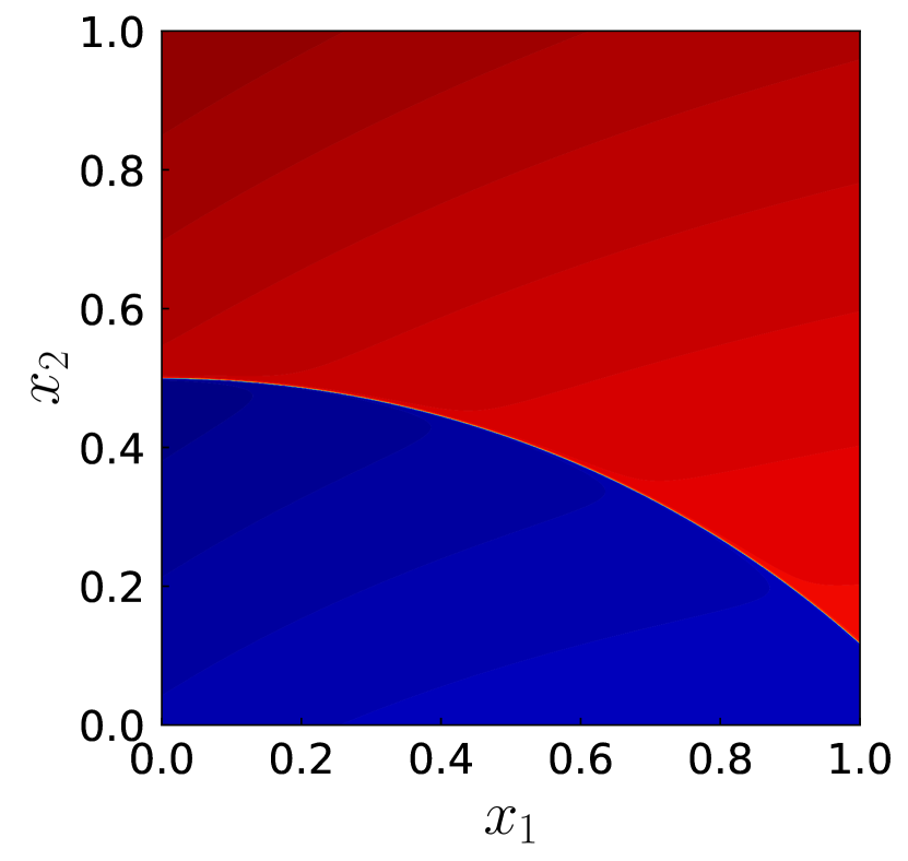
where δ𝛿\delta is a parameter that controls the stiffness of the internal boundary layer (see Figure 2). In this example, we set δ=0.01𝛿0.01\delta=0.01 to obtain a smooth solution to assess the expected convergence rates. In addition, we apply the adaptive strategy from (38) to solve this problem using the a-posteriori residual estimate of [10] and the residual minimization error estimate to guide the adaptivity from the same initial mesh (see Figure 3(a)).

Refer to caption
(a) δ=0.01𝛿0.01\delta=0.01
Refer to caption
(b) δ=0.001𝛿0.001\delta=0.001
Refer to caption
(c) δ=0.0001𝛿0.0001\delta=0.0001
Figure 2: 2D advection-reaction problem (exact solution)

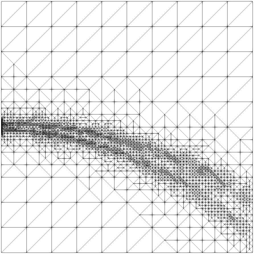
Figures 3(b) and 3(c) compare the refined meshes resulting from residual-based and a-posteriori estimates at similar numbers of degrees of freedom (DoFs)DoFs(\textrm{DoFs}). The a-posteriori estimate focuses the mesh refinement at the outflow boundary and the interior layer, with less emphasis at the inflow boundary. The residual-based estimator concentrates the refinement at the inflow boundary and progressively solves the interior layer.

Refer to caption
(a) Initial mesh
Refer to caption
(b) Residual-based estimator (143,270 DoF)
Refer to caption
(c) A-posteriori estimator (145,720 DoF)
Figure 3: Initial & refined meshes for similar total degrees-of-freedom (DoF) number using residual-based & a-posterior estimator from [10]

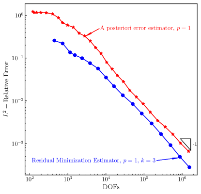
Figure 4 shows the comparison of the L2superscript𝐿2L^{2}-relative error between the a posteriori error estimate proposed in [10] (red curve) and the residual-based estimate (blue curve). For the residual minimization scheme, we choose a piecewise continuous trial space of order p=1𝑝1p=1 and its enrichment with bubbles of order k=p+2𝑘𝑝2k=p+2 as a test space. As for the a-posteriori error estimation strategy, we use conforming piecewise continuous trial and test space of order p=1𝑝1p=1 [10]. We plot all quantities against the total number of degrees of freedom (DoFs), and the triangle shows the slope DoFs1superscriptDoFs1\textrm{DoFs}^{-1}, which is the optimal convergence in the L2superscript𝐿2L^{2}-norm for smooth problems [10]. The convergence rate of the CIP formulation that uses the residual minimization strategy over a bubble-enriched test space is slightly better than the one obtained from applying the CIP method with the a-posteriori error estimation strategy. In addition, note, in particular, the superconvergence of the L2superscript𝐿2L^{2}-error using CIP and residual minimization method when the mesh enters the asymptotic range. This is meaningful since the residual error estimate is defined in the energy norm. Although the convergence rate is improved in the L2superscript𝐿2L^{2}-norm the total number of DoFs using residual minimization is greater than the DoFs using the strategy in [10]. This fact is because residual minimization solves a full saddle-point system that gives a discrete solution and a residual estimate in the bubble-enriched test space.
Refer to caption
Figure 4: L2superscript𝐿2L^{2}-relative error (uuhΩuΩ)subscriptnorm𝑢subscript𝑢Ωsubscriptnorm𝑢Ω\left(\frac{\|u-u_{h}\|_{\Omega}}{\|u\|_{\Omega}}\right). A-posteriori estimator of [10] and residual-based estimate.

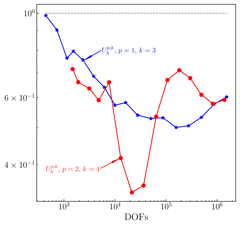
Next, we study the validity of the saturation assumption (see Assumption 3) by considering the triple norm ||||||h,k{\left|\kern-1.07639pt\left|\kern-1.07639pt\left|\cdot\right|\kern-1.07639pt\right|\kern-1.07639pt\right|}_{h,k} from (21) and introduce the following ratio,

𝒮:=|uθh|h,k|uuh|h,k.assign𝒮subscriptnorm𝑢subscript𝜃𝑘subscriptnorm𝑢subscript𝑢𝑘\mathcal{S}:=\dfrac{{\left|\kern-1.07639pt\left|\kern-1.07639pt\left|u-\theta_{h}\right|\kern-1.07639pt\right|\kern-1.07639pt\right|}_{h,k}}{{\left|\kern-1.07639pt\left|\kern-1.07639pt\left|u-u_{h}\right|\kern-1.07639pt\right|\kern-1.07639pt\right|}_{h,k}}. (39)

When 𝒮<1𝒮1\mathcal{S}<1, the approximation satisfies the saturation assumption 3. Figure 5 shows the residual representative’s robustness and saturation assumption (i.e., Assumption 3) using piecewise continuous trial space of order p=1𝑝1p=1 and p=2𝑝2p=2 and test space as its enrichment with bubbles of order k=p+2𝑘𝑝2k=p+2. Figure 5(a) shows that |εh|h,ksubscriptnormsubscript𝜀𝑘{\left|\kern-1.07639pt\left|\kern-1.07639pt\left|\varepsilon_{h}\right|\kern-1.07639pt\right|\kern-1.07639pt\right|}_{h,k} is robust as it is a lower bound of |uuh|h,ksubscriptnorm𝑢subscript𝑢𝑘{\left|\kern-1.07639pt\left|\kern-1.07639pt\left|u-u_{h}\right|\kern-1.07639pt\right|\kern-1.07639pt\right|}_{h,k} (see Proposition 2). In addition, the saturation Assumption 3 also holds even in the pre-asymptotic regime (see Figure 5(b)).

Refer to caption
(a) Residual estimator robustness
Refer to caption
(b) Saturation
Figure 5: Relative error in the triple norm ||||||h,k{\left|\kern-0.96873pt\left|\kern-0.96873pt\left|\cdot\right|\kern-0.96873pt\right|\kern-0.96873pt\right|}_{h,k} & saturation assumption.

5.2 Goal-oriented adaptivity for advection-reaction problems

Following [49], we perform Goal-Oriented Adaptivity (GoA). The key insight behind this theory is to consider an adjoint continuous formulation and an adjoint problem to the saddle-point formulation (29). Thus, we approximate a quantity of interest (QoI) q(u)𝑞𝑢q(u), where q:U:𝑞maps-to𝑈q:U\mapsto\mathbb{R} is a bounded linear functional and uU𝑢𝑈u\in U is the exact solution of the continuous problem (6). The GoA strategy of [49] solves an additional continuous adjoint problem, which is equivalent to solving the following saddle-point problem as the adjoint formulation of problem (29):

{Find (νh,wh)Uhp,k×Uhp, such that:(νh,νh)Uhp,k+bh(wh,νh)= 0,νhUhp,k,bh(wh,νh)=q(wh),whUhp,casesFind subscriptsuperscript𝜈subscriptsuperscript𝑤subscriptsuperscript𝑈𝑝𝑘subscriptsuperscript𝑈𝑝 such that:subscriptsubscriptsuperscript𝜈subscript𝜈subscriptsuperscript𝑈𝑝𝑘subscript𝑏subscriptsuperscript𝑤subscript𝜈absent 0for-allsubscript𝜈subscriptsuperscript𝑈𝑝𝑘subscript𝑏subscript𝑤subscriptsuperscript𝜈absent𝑞subscript𝑤for-allsubscript𝑤subscriptsuperscript𝑈𝑝\left\{\begin{array}[]{l}\text{Find }(\nu^{*}_{h},w^{*}_{h})\in U^{p,k}_{h}\times U^{p}_{h},\text{ such that:}\\ \begin{array}[]{lll}(\nu^{*}_{h},\,\nu_{h})_{U^{p,k}_{h}}+b_{h}(w^{*}_{h},\,\nu_{h})&=\ 0,&\quad\forall\,\nu_{h}\in U^{p,k}_{h},\\ b_{h}(w_{h},\,\nu^{*}_{h})&=\ q(w_{h}),&\quad\forall\,w_{h}\in U^{p}_{h},\end{array}\end{array}\right. (40)

where νhUhp,ksubscriptsuperscript𝜈subscriptsuperscript𝑈𝑝𝑘\nu^{*}_{h}\in U^{p,k}_{h} approximates the discrete solution of the adjoint continuous problem (see [49]); the adjoint counterpart of the solution uhUhpsubscript𝑢subscriptsuperscript𝑈𝑝u_{h}\in U^{p}_{h} of (29) while whUhpsubscriptsuperscript𝑤subscriptsuperscript𝑈𝑝w^{*}_{h}\in U^{p}_{h} is an additional variable that constrains the solution dimension. Moreover, as the direct saddle-point problem (29) is well-posed, the adjoint saddle-point problem (40) is also well-posed; the two problems share the same left-hand side. Thus, we approximate the error in the QoI following [49], which solves an auxiliary discrete problem that has a unique solution and is well-posed,

{Find εhUhp,k such that:(εh,νh)=q(νh)bh(νh,νh),νhUhp,kcasesFind subscriptsuperscript𝜀subscriptsuperscript𝑈𝑝𝑘 such that:formulae-sequencesubscriptsuperscript𝜀subscript𝜈𝑞subscript𝜈subscript𝑏subscript𝜈subscriptsuperscript𝜈for-allsubscript𝜈subscriptsuperscript𝑈𝑝𝑘\left\{\begin{array}[]{l}\text{Find }\varepsilon^{*}_{h}\in U^{p,k}_{h}\,\text{ such that:}\\ (\varepsilon^{*}_{h},\nu_{h})=q(\nu_{h})-b_{h}(\nu_{h},\nu^{*}_{h}),\quad\forall\,\nu_{h}\in U^{p,k}_{h}\end{array}\right. (41)

We adopt the following adjoint-residual-based estimator for the QoI [49],

𝔼T2(εh,εh):=|(εh,εh)Uhp,k|assignsubscriptsuperscript𝔼2𝑇subscript𝜀subscriptsuperscript𝜀subscriptsubscript𝜀subscriptsuperscript𝜀subscriptsuperscript𝑈𝑝𝑘\mathbb{E}^{2}_{T}(\varepsilon_{h},\varepsilon^{*}_{h}):=\big{|}\big{(}\varepsilon_{h},\varepsilon^{*}_{h}\big{)}_{U^{p,k}_{h}}\big{|} (42)

which solves (29) and (40) along with the adjoint residual problem (41). Then, we mark each element with its local upper bound |εh|Th,k|εh|Th,ksubscriptnormsubscript𝜀subscript𝑇𝑘subscriptnormsubscriptsuperscript𝜀subscript𝑇𝑘{\left|\kern-1.07639pt\left|\kern-1.07639pt\left|\varepsilon_{h}\right|\kern-1.07639pt\right|\kern-1.07639pt\right|}_{T_{h,k}}{\left|\kern-1.07639pt\left|\kern-1.07639pt\left|\varepsilon^{*}_{h}\right|\kern-1.07639pt\right|\kern-1.07639pt\right|}_{T_{h,k}} where ||||||Th,k{\left|\kern-1.07639pt\left|\kern-1.07639pt\left|\cdot\right|\kern-1.07639pt\right|\kern-1.07639pt\right|}_{T_{h,k}} is the element localized triple norm. Rojas et al. [49] built the theory using a dG framework; nevertheless, it is general and can be applied to the bubble-enriched continuous test spaces as well. In our numerical example, we consider the advection-reaction problem (6) over the unit square domain Ω=[0, 1]22Ωsuperscript012superscript2\Omega=[0,\,1]^{2}\in\mathbb{R}^{2}, with a constant velocity field b=(3,1)T𝑏superscript31𝑇b=(3,1)^{T} (cf. [49]). Let the reaction parameter be μ=0𝜇0\mu=0 (advection dominated), thus the source term is f=μu=0𝑓𝜇𝑢0f=\mu\,u=0 in ΩΩ\Omega. In this case, g(x1,x2)𝑔subscript𝑥1subscript𝑥2g(x_{1},x_{2}) defines the exact solution as,

u(x1,x2)=2+tanh(10(x2x1314))+tanh(1000(x2x1334)).𝑢subscript𝑥1subscript𝑥2210subscript𝑥2subscript𝑥13141000subscript𝑥2subscript𝑥1334u(x_{1},x_{2})=2+\tanh\left(10\left(x_{2}-\dfrac{x_{1}}{3}-\dfrac{1}{4}\right)\right)+\tanh\left(1000\left(x_{2}-\dfrac{x_{1}}{3}-\dfrac{3}{4}\right)\right). (43)
Refer to caption
(a) Initial mesh
Refer to caption
(b) Bubble-enriched CIP (110,990 DoF)
Refer to caption
(c) dG framework (107,040 DoF)
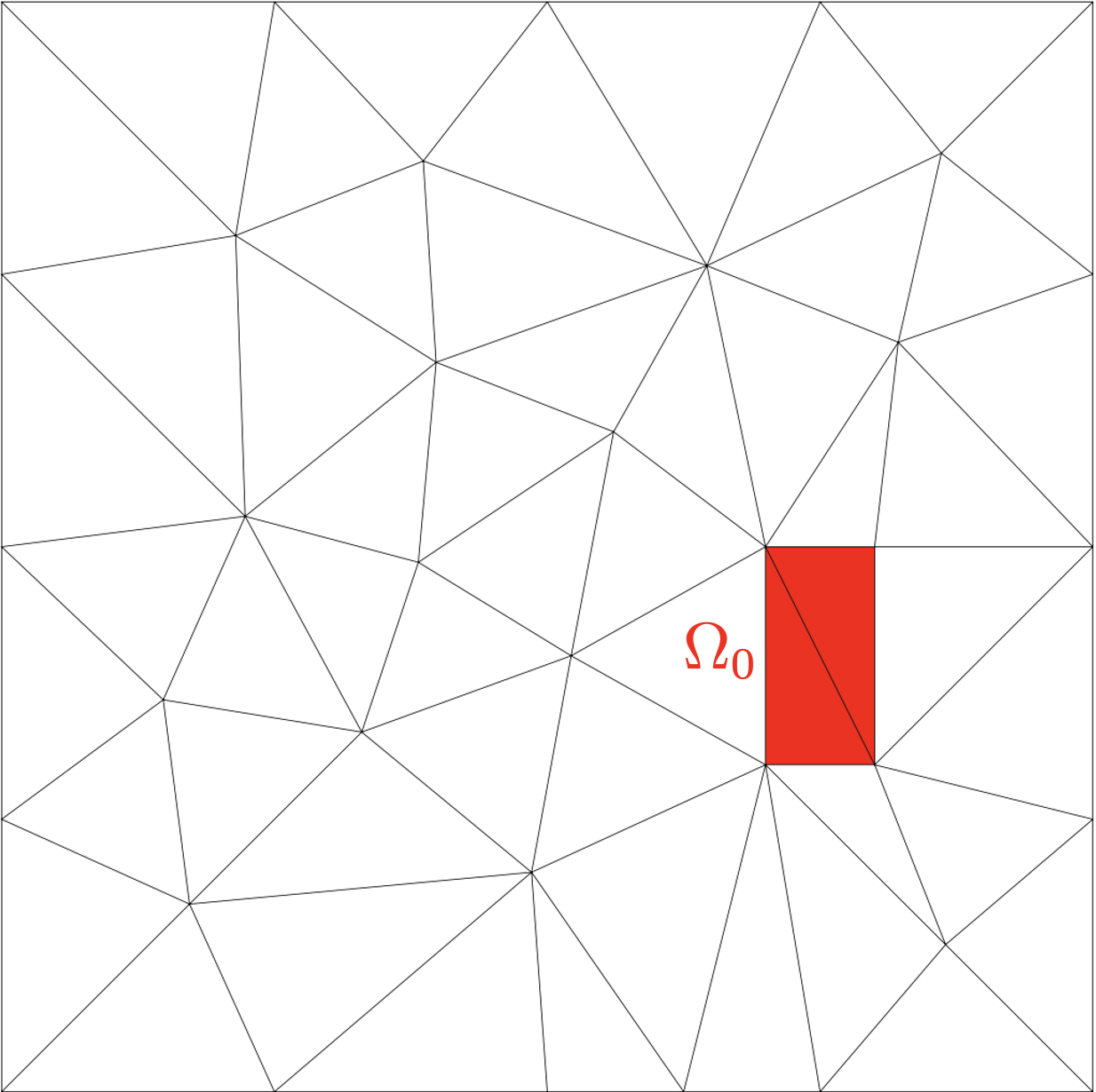
Figure 6: Initial & refined meshes for similar total degrees-of-freedom DoF number using CIP formulation with a bubble enriched test space (p=1,k=3)formulae-sequence𝑝1𝑘3(p=1,\,k=3) & a dG framework (p=1,Δp=0)formulae-sequence𝑝1Δ𝑝0(p=1,\,\Delta p=0)
Refer to caption
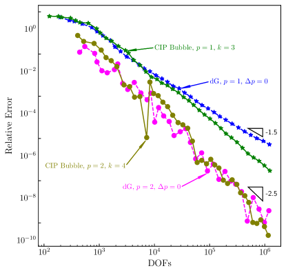
Figure 7: Relative error (|q(uuh)|/|q(u)|(|q(u-u_{h})|/|q(u)| in the quantity of interest (QoI) using residual minimization with a CIP formulation with bubble-enriched test space (solid lines) and a dG framework (dashed lines)

In addition, the QoI has the following form,

q(u)=1|Ω0|Ω0u𝑑Ω0,𝑞𝑢1subscriptΩ0subscriptsubscriptΩ0𝑢differential-dsubscriptΩ0q(u)=\dfrac{1}{|\Omega_{0}|}\int_{\Omega_{0}}ud\Omega_{0}, (44)

where u𝑢u is the exact solution (43) and Ω0=(0.7,0.8)×(0.3,0.5)subscriptΩ00.70.80.30.5\Omega_{0}=(0.7,0.8)\times(0.3,0.5) is a subdomain of the physical domain ΩΩ\Omega. As the starting point for the adaptive procedure, we consider the Ω0subscriptΩ0\Omega_{0}-conforming mesh of Figure 6(a). Figure 6 displays the resulting adapted meshes using a CIP formulation with bubble-enriched test space and a dG framework at a similar total number of DoFs. These figures show that the resulting adapted meshes are similar, and both methodologies adjust the refinement process consistently to the physical problem nature. Next, we compare error plots against the expected optimal convergence slope DoF(p+12)superscriptDoF𝑝12\textrm{DoF}^{-\left(p+\frac{1}{2}\right)} where p𝑝p is the polynomial order of the trial space (see [32]). Since the error is measured in a QoI, we compare the results obtained in [49] using a dG framework against CIP method with residual minimization onto a bubble-enriched test space results directly. We evaluate the numerical results considering two polynomial orders for the trial space (namely p=1, 2𝑝12p=1,\,2) with the same polynomial order for the dG test space (i.e., Δp=0Δ𝑝0\Delta p=0) and k=p+2𝑘𝑝2k=p+2 for bubble enriched test space. Figure 7 shows the convergence of the relative error in the QoI for the CIP formulation with residual minimization onto bubble-enriched test spaces (solid lines) and the dG framework proposed in [49] (dashed lines). For low order approximations, the CIP formulation with residual minimization shows super convergence compared to the residual minimization using a dG test space that achieves the optimal convergence rate. For higher-order polynomial spaces, CIP has a performance similar to the dG framework.

6 Contributions and future work.

This paper extends AS-FEM to use the hp𝑝hp-CIP finite element method with an enriched test space. We use a stable formulation (namely, the CIP formulation) in the trial space and enlarge the test space via bubble enrichment of the trial space to estimate a residual representative to guide adaptivity, see [42]. This is meaningful as, in this case, the formulation is already stable in the trial space. Since we choose the coercive stable CIP formulation, we derive a new a-priori error estimate result for the residual minimization method using continuous bubble-enriched test spaces, which relies on an orthogonality argument for the boundedness of the discrete bilinear form that proves quasi-optimal convergence for advection-reaction problems. We also confirm numerically that the residual estimate is robust regarding the energy norm and competitive with the a-posteriori error estimate available in the literature. Moreover, we show that using the CIP formulation and residual minimization onto bubble-enriched test spaces improves the convergence rates in the L2superscript𝐿2L^{2}-norm. However, the residual estimator is calculated using the energy norm. The numerical results for goal-oriented adaptivity suggest that applying residual minimization and a coercive stable formulation using bubble-enriched continuous test spaces improves convergence rates for the error in the quantity of interest when the polynomial order for the trial space is low. Additionally, the method maintains the optimal convergence rates for high-order spaces. Further research will explore the performance of this method applied to other challenging problems. For example, we will study the extension of this method to non-linear hyperbolic equations that describe many engineering problems, such as solving the shallow water equations and coupled fluid and solid mechanics equations for assessing the long-term stability of tailing dams.

Acknowledments

This publication was made possible in part by the support of Vista Energy Company, which promoted the exploration of new numerical techniques for simulating industry-related problems. Additionally, this publication was made possible in part by the Professorial Chair in Computational Geoscience at Curtin University. This project has received funding from the European Union’s Horizon 2020 research and innovation programme under the Marie Sklodowska-Curie grant agreement No 777778 (MATHROCKS).

Appendix A Proof of Proposition 1.

We separate the proof of Proposition 1 into two part: Lemma 7 and Theorem 2, with the a-priori error estimate onto bubble enrichment.

Lemma 7 (Boundedness).

Consider k=p+1>d=2𝑘𝑝1𝑑2k=p+1>d=2. If η(Uhp):={zL2(Ω):(z,νh)=0,νhUhp}𝜂superscriptsubscriptsuperscript𝑈𝑝perpendicular-toassignconditional-set𝑧superscript𝐿2Ωformulae-sequence𝑧subscript𝜈0for-allsubscript𝜈subscriptsuperscript𝑈𝑝~{}\eta\in\left(U^{p}_{h}\right)^{\perp}:=\left\{z\in L^{2}(\Omega):(z,\nu_{h})=0,\,\forall\nu_{h}\in U^{p}_{h}\right\} the following result holds,

supνhUhp,kbh(η,νh)|νh|k,h|η|k,h,#,less-than-or-similar-tosubscript𝜈subscriptsuperscript𝑈𝑝𝑘supremumsubscript𝑏𝜂subscript𝜈subscriptnormsubscript𝜈𝑘subscriptnorm𝜂𝑘#\underset{\nu_{h}\in U^{p,k}_{h}}{\sup}\dfrac{b_{h}(\eta,\nu_{h})}{{\left|\kern-1.07639pt\left|\kern-1.07639pt\left|\nu_{h}\right|\kern-1.07639pt\right|\kern-1.07639pt\right|}_{k,h}}\lesssim{\left|\kern-1.07639pt\left|\kern-1.07639pt\left|\eta\right|\kern-1.07639pt\right|\kern-1.07639pt\right|}_{k,h,\#}, (45)

where the norm

|η|k,h,#:=|η|k,h+(k2h12p1/2+kα/2p1/2)|η|hassignsubscriptnorm𝜂𝑘#subscriptnorm𝜂𝑘superscript𝑘2superscript12superscript𝑝12superscript𝑘𝛼2superscript𝑝12subscript𝜂{\left|\kern-1.07639pt\left|\kern-1.07639pt\left|\eta\right|\kern-1.07639pt\right|\kern-1.07639pt\right|}_{k,h,\#}:={\left|\kern-1.07639pt\left|\kern-1.07639pt\left|\eta\right|\kern-1.07639pt\right|\kern-1.07639pt\right|}_{k,h}+\big{(}k^{2}\,h^{\frac{1}{2}}p^{1/2}+k^{\alpha/2}p^{-1/2}\big{)}|\eta|_{h}

and ||h,|\cdot|_{h}, is the semi-norm

|η|h:=(TΩhhT1βT,ηT2)1/2.assignsubscript𝜂superscriptsubscript𝑇subscriptΩsubscriptsuperscript1𝑇subscript𝛽𝑇subscriptsuperscriptnorm𝜂2𝑇12|\eta|_{h}:=\left(\sum_{T\in\Omega_{h}}h^{-1}_{T}\beta_{T,\infty}\|\eta\|^{2}_{T}\right)^{1/2}.
Proof.

The only term to estimate in (22) is (η,bνh)Ωsubscript𝜂bsubscript𝜈Ω\big{(}\eta,\,\textbf{b}\cdot\nabla\nu_{h}\big{)}_{\Omega}. Let bhsubscriptb\textbf{b}_{h} the L2superscript𝐿2L^{2}-orthogonal projection of b onto Vh0superscriptsubscript𝑉0V_{h}^{0}. Thus,

(η,bνh)Ω=(η,(bbh)νh)Ω+(η,bhνh)Ω.subscript𝜂bsubscript𝜈Ωsubscript𝜂bsubscriptbsubscript𝜈Ωsubscript𝜂subscriptbsubscript𝜈Ω\big{(}\eta,\textbf{b}\cdot\nabla\nu_{h}\big{)}_{\Omega}=\big{(}\eta,(\textbf{b}-\textbf{b}_{h})\cdot\nabla\nu_{h}\big{)}_{\Omega}+\big{(}\eta,\textbf{b}_{h}\nabla\nu_{h}\big{)}_{\Omega}. (46)

Since b[W1,(Ω)]2bsuperscriptdelimited-[]superscript𝑊1Ω2\textbf{b}\in\big{[}W^{1,\infty}(\Omega)\big{]}^{2}, and νhUhp,kUhksubscript𝜈superscriptsubscript𝑈𝑝𝑘superscriptsubscript𝑈𝑘\nu_{h}\in U_{h}^{p,k}\subset U_{h}^{k} we have the following inverse inequalities (see e.g., [17]):

bbh[L(T)]dsubscriptnormbsubscriptbsuperscriptdelimited-[]superscript𝐿𝑇𝑑\displaystyle\|\textbf{b}-\textbf{b}_{h}\|_{[L^{\infty}(T)]^{d}} hTb[W1,(T)]d,less-than-or-similar-toabsentsubscript𝑇subscriptnormbsuperscriptdelimited-[]superscript𝑊1𝑇𝑑\displaystyle\lesssim h_{T}\|\textbf{b}\|_{[W^{1,\infty}(T)]^{d}}, (47)
vhTsubscriptnormsubscript𝑣𝑇\displaystyle\|\nabla v_{h}\|_{T} k2hT1vhT, for allTΩh.formulae-sequenceless-than-or-similar-toabsentsuperscript𝑘2subscriptsuperscript1𝑇subscriptnormsubscript𝑣𝑇 for all𝑇subscriptΩ\displaystyle\lesssim k^{2}h^{-1}_{T}\|v_{h}\|_{T},\text{ for all}T\in\Omega_{h}. (48)

Thus, we can bound the first term in the right-hand side of (46) as follows:

(η,(bbh)νh)Ωsubscript𝜂bsubscriptbsubscript𝜈Ω\displaystyle\big{(}\eta,(\textbf{b}-\textbf{b}_{h})\cdot\nabla\nu_{h}\big{)}_{\Omega} (TΩhhT1βT,ηT2)12(TΩhhT3βT,1bW1,(T)2νhT2)12(by (47) and Cauchy-Schwartz)less-than-or-similar-toabsentsuperscriptsubscript𝑇subscriptΩsuperscriptsubscript𝑇1subscript𝛽𝑇subscriptsuperscriptnorm𝜂2𝑇12superscriptsubscript𝑇subscriptΩsuperscriptsubscript𝑇3superscriptsubscript𝛽𝑇1superscriptsubscriptnormbsuperscript𝑊1𝑇2superscriptsubscriptnormsubscript𝜈𝑇212(by (47) and Cauchy-Schwartz)\displaystyle\lesssim\left(\sum_{T\in\Omega_{h}}h_{T}^{-1}\beta_{T,\infty}{\left|\kern-1.07639pt\left|\eta\right|\kern-1.07639pt\right|}^{2}_{T}\right)^{\frac{1}{2}}\left(\sum_{T\in\Omega_{h}}h_{T}^{3}\beta_{T,\infty}^{-1}{\left|\kern-1.07639pt\left|\textbf{b}\right|\kern-1.07639pt\right|}_{W^{1,\infty}(T)}^{2}{\left|\kern-1.07639pt\left|\nabla\nu_{h}\right|\kern-1.07639pt\right|}_{T}^{2}\right)^{\frac{1}{2}}\quad\text{(by~{}\eqref{eq:inverseW1} and Cauchy-Schwartz)}
k2h12|η|hνhΩ(by (35), and (48)).less-than-or-similar-toabsentsuperscript𝑘2superscript12subscript𝜂subscriptnormsubscript𝜈Ω(by (35), and (48))\displaystyle\lesssim k^{2}h^{\frac{1}{2}}|\eta|_{h}{\left|\kern-1.07639pt\left|\nu_{h}\right|\kern-1.07639pt\right|}_{\Omega}\hskip 174.41553pt\ \text{(by~{}\eqref{eq:semi-norm}, and~{}\eqref{eq:inverseL2})}.

The second term in the right-hand side of (46) is estimated using the fact that η(Uhp)𝜂superscriptsubscriptsuperscript𝑈𝑝perpendicular-to\eta\in\left(U^{p}_{h}\right)^{\perp}, the Cauchy-Schwartz inequality and the interpolation estimate of Lemma 2. Let ϕh:=bhνhassignsubscriptitalic-ϕsubscriptbsubscript𝜈\phi_{h}:=\textbf{b}_{h}\cdot\nabla\nu_{h}. We call Uβ,h:={IOs(ϕh):ϕh=bhνh,νhUhk,p}.assignsubscript𝑈𝛽conditional-setsubscript𝐼𝑂𝑠subscriptitalic-ϕformulae-sequencesubscriptitalic-ϕsubscriptbsubscript𝜈subscript𝜈subscriptsuperscript𝑈𝑘𝑝U_{\beta,h}:=\left\{I_{Os}(\phi_{h}):\phi_{h}=\textbf{b}_{h}\cdot\nabla\nu_{h},\quad\nu_{h}\in U^{k,p}_{h}\right\}. Since, IOsϕhsubscript𝐼𝑂𝑠subscriptitalic-ϕI_{Os}\phi_{h} may not be in Uhp,ksubscriptsuperscript𝑈𝑝𝑘U^{p,k}_{h} but it is contained in Uhpsubscriptsuperscript𝑈𝑝U^{p}_{h}, since k=p+1𝑘𝑝1k=p+1. Hence,

(η,ϕh)Ωsubscript𝜂subscriptitalic-ϕΩ\displaystyle\big{(}\eta,\phi_{h})_{\Omega} =(η,ϕhIOsϕh)Ωabsentsubscript𝜂subscriptitalic-ϕsubscript𝐼𝑂𝑠subscriptitalic-ϕΩ\displaystyle=\big{(}\eta,\phi_{h}-I_{Os}\phi_{h}\big{)}_{\Omega}
(TΩhhT1βT,ηT2)12(TΩhhTβT,1ϕIOsϕhT2)12absentsuperscriptsubscript𝑇subscriptΩsuperscriptsubscript𝑇1subscript𝛽𝑇subscriptsuperscriptnorm𝜂2𝑇12superscriptsubscript𝑇subscriptΩsubscript𝑇superscriptsubscript𝛽𝑇1subscriptsuperscriptnormitalic-ϕsubscript𝐼𝑂𝑠subscriptitalic-ϕ2𝑇12\displaystyle\leq\left(\sum_{T\in\Omega_{h}}h_{T}^{-1}\beta_{T,\infty}{\left|\kern-1.07639pt\left|\eta\right|\kern-1.07639pt\right|}^{2}_{T}\right)^{\frac{1}{2}}\left(\sum_{T\in\Omega_{h}}h_{T}\beta_{T,\infty}^{-1}{\left|\kern-1.07639pt\left|\phi-I_{Os}\phi_{h}\right|\kern-1.07639pt\right|}^{2}_{T}\right)^{\frac{1}{2}}
|η|h(TΩheThT2p1βT,1\llbracketϕh\rrbrackete2)12.less-than-or-similar-toabsentsubscript𝜂superscriptsubscript𝑇subscriptΩsubscript𝑒subscript𝑇superscriptsubscript𝑇2superscript𝑝1superscriptsubscript𝛽𝑇1subscriptsuperscriptnorm\llbracketsubscriptitalic-ϕ\rrbracket2𝑒12\displaystyle\lesssim|\eta|_{h}\left(\sum_{T\in\Omega_{h}}\sum_{e\in\mathcal{F}_{T}}h_{T}^{2}p^{-1}\beta_{T,\infty}^{-1}{\left|\kern-1.07639pt\left|\llbracket\phi_{h}\rrbracket\right|\kern-1.07639pt\right|}^{2}_{e}\right)^{\frac{1}{2}}.

Since

\llbracketϕh\rrbrackete=\llbracketbhνh\rrbrackete\llbracket(bbh)νh\rrbrackete+\llbracketbνh\rrbrackete,subscriptnorm\llbracketsubscriptitalic-ϕ\rrbracket𝑒subscriptnorm\llbracketsubscriptbsubscript𝜈\rrbracket𝑒less-than-or-similar-tosubscriptnorm\llbracketbsubscriptbsubscript𝜈\rrbracket𝑒subscriptnorm\llbracketbsubscript𝜈\rrbracket𝑒\displaystyle{\left|\kern-1.07639pt\left|\llbracket\phi_{h}\rrbracket\right|\kern-1.07639pt\right|}_{e}={\left|\kern-1.07639pt\left|\llbracket\textbf{b}_{h}\cdot\nabla\nu_{h}\rrbracket\right|\kern-1.07639pt\right|}_{e}\lesssim{\left|\kern-1.07639pt\left|\llbracket(\textbf{b}-\textbf{b}_{h})\cdot\nabla\nu_{h}\rrbracket\right|\kern-1.07639pt\right|}_{e}+{\left|\kern-1.07639pt\left|\llbracket\textbf{b}\cdot\nabla\nu_{h}\rrbracket\right|\kern-1.07639pt\right|}_{e}, (49)

and

\llbracket(bbh)νh\rrbracketesubscriptnorm\llbracketbsubscriptbsubscript𝜈\rrbracket𝑒\displaystyle{\left|\kern-1.07639pt\left|\llbracket(\textbf{b}-\textbf{b}_{h})\cdot\nabla\nu_{h}\rrbracket\right|\kern-1.07639pt\right|}_{e} eT¯hTb[W1,(T)]dνh|Teless-than-or-similar-toabsentevaluated-atsubscript𝑒¯𝑇subscript𝑇subscriptnormbsuperscriptdelimited-[]superscript𝑊1𝑇𝑑subscriptdelimited-‖|subscript𝜈𝑇𝑒\displaystyle\lesssim\sum_{e\in\overline{T}}h_{T}\|\textbf{b}\|_{[W^{1,\infty}(T)]^{d}}\|\nabla\nu_{h}|_{T}\|_{e} (50)
eT¯hTb[W1,(T)]d(p2hT)1/2νhTless-than-or-similar-toabsentsubscript𝑒¯𝑇subscript𝑇subscriptnormbsuperscriptdelimited-[]superscript𝑊1𝑇𝑑superscriptsuperscript𝑝2subscript𝑇12subscriptnormsubscript𝜈𝑇\displaystyle\lesssim\sum_{e\in\overline{T}}h_{T}\|\textbf{b}\|_{[W^{1,\infty}(T)]^{d}}\left(\frac{p^{2}}{h_{T}}\right)^{1/2}\|\nabla\nu_{h}\|_{T} ( Estimate (14)) (51)
eT¯hTb[W1,(T)]d(p2hT)1/2k2hTνhTless-than-or-similar-toabsentsubscript𝑒¯𝑇subscript𝑇subscriptnormbsuperscriptdelimited-[]superscript𝑊1𝑇𝑑superscriptsuperscript𝑝2subscript𝑇12superscript𝑘2subscript𝑇subscriptnormsubscript𝜈𝑇\displaystyle\lesssim\sum_{e\in\overline{T}}h_{T}\|\textbf{b}\|_{[W^{1,\infty}(T)]^{d}}\left(\frac{p^{2}}{h_{T}}\right)^{1/2}\frac{k^{2}}{h_{T}}\|\nu_{h}\|_{T} (Estimate (48)) (52)
eT¯b[W1,(T)]dpk2hT1/2νhT.less-than-or-similar-toabsentsubscript𝑒¯𝑇subscriptnormbsuperscriptdelimited-[]superscript𝑊1𝑇𝑑𝑝superscript𝑘2superscriptsubscript𝑇12subscriptnormsubscript𝜈𝑇\displaystyle\lesssim\sum_{e\in\overline{T}}\|\textbf{b}\|_{[W^{1,\infty}(T)]^{d}}\frac{pk^{2}}{h_{T}^{1/2}}\|\nu_{h}\|_{T}. (53)

Hence

TΩheThT2p1βT,1\llbracket(bbh)vh\rrbrackete2pk4hvhΩ2less-than-or-similar-tosubscript𝑇subscriptΩsubscript𝑒subscript𝑇superscriptsubscript𝑇2superscript𝑝1superscriptsubscript𝛽𝑇1subscriptsuperscriptnorm\llbracketbsubscriptbsubscript𝑣\rrbracket2𝑒𝑝superscript𝑘4superscriptsubscriptnormsubscript𝑣Ω2\displaystyle\sum_{T\in\Omega_{h}}\sum_{e\in\mathcal{F}_{T}}h_{T}^{2}p^{-1}\beta_{T,\infty}^{-1}{\left|\kern-1.07639pt\left|\llbracket(\textbf{b}-\textbf{b}_{h})\cdot\nabla v_{h}\rrbracket\right|\kern-1.07639pt\right|}^{2}_{e}\lesssim{p}k^{4}h\|v_{h}\|_{\Omega}^{2}

Furthermore,

TΩheThT2p1βT,1\llbracketbνh\rrbrackete2subscript𝑇subscriptΩsubscript𝑒subscript𝑇superscriptsubscript𝑇2superscript𝑝1superscriptsubscript𝛽𝑇1subscriptsuperscriptnorm\llbracketbsubscript𝜈\rrbracket2𝑒\displaystyle\sum_{T\in\Omega_{h}}\sum_{e\in\mathcal{F}_{T}}h_{T}^{2}p^{-1}\beta_{T,\infty}^{-1}{\left|\kern-1.07639pt\left|\llbracket\textbf{b}\cdot\nabla\nu_{h}\rrbracket\right|\kern-1.07639pt\right|}^{2}_{e} TΩheThe2p1βe,\llbracketvhn\rrbrackete2less-than-or-similar-toabsentsubscript𝑇subscriptΩsubscript𝑒subscript𝑇superscriptsubscript𝑒2superscript𝑝1subscript𝛽𝑒superscriptsubscriptnorm\llbracketsubscript𝑣𝑛\rrbracket𝑒2\displaystyle\lesssim\sum_{T\in\Omega_{h}}\sum_{e\in\mathcal{F}_{T}}h_{e}^{2}p^{-1}\beta_{e,\infty}{\left|\kern-1.07639pt\left|\llbracket\nabla v_{h}\cdot n\rrbracket\right|\kern-1.07639pt\right|}_{e}^{2} (54)
p1kαj(vh,vh).less-than-or-similar-toabsentsuperscript𝑝1superscript𝑘𝛼𝑗subscript𝑣subscript𝑣\displaystyle\lesssim p^{-1}k^{\alpha}j(v_{h},v_{h}). (55)

Collecting the above estimates and Lemma 5 yields

(η,ϕh)Ω|η|h(k2h12p1/2+kα/2p1/2)|νh|k,h.less-than-or-similar-tosubscript𝜂subscriptitalic-ϕΩsubscript𝜂superscript𝑘2superscript12superscript𝑝12superscript𝑘𝛼2superscript𝑝12subscriptnormsubscript𝜈𝑘\big{(}\eta,\phi_{h}\big{)}_{\Omega}\lesssim|\eta|_{h}\big{(}k^{2}\,h^{\frac{1}{2}}p^{1/2}+k^{\alpha/2}p^{-1/2}\big{)}{\left|\kern-1.07639pt\left|\kern-1.07639pt\left|\nu_{h}\right|\kern-1.07639pt\right|\kern-1.07639pt\right|}_{k,h}.

This completes the proof. ∎

Lemma 8.

Consider the continuous L2(Ω)superscript𝐿2ΩL^{2}(\Omega)-projection operator Πh:L2(Ω)Uhp:subscriptΠsuperscript𝐿2Ωsuperscriptsubscript𝑈𝑝\Pi_{h}:L^{2}(\Omega)\to U_{h}^{p}. Then, for all wHs(Ω)𝑤superscript𝐻𝑠Ωw\in H^{s}(\Omega), s1𝑠1s\geq 1, we have the following hp𝑝hp-approximation properties

|wΠhw|hsubscript𝑤subscriptΠ𝑤\displaystyle|w-\Pi_{h}w|_{h} p14(hp)q1/2wq,Ω,less-than-or-similar-toabsentsuperscript𝑝14superscript𝑝𝑞12subscriptnorm𝑤𝑞Ω\displaystyle\lesssim p^{-\frac{1}{4}}\left(\frac{h}{p}\right)^{q-1/2}\|w\|_{q,\Omega}, (56)
|wΠhw|h,ksubscriptnorm𝑤subscriptΠ𝑤𝑘\displaystyle{\left|\kern-1.07639pt\left|\kern-1.07639pt\left|w-\Pi_{h}w\right|\kern-1.07639pt\right|\kern-1.07639pt\right|}_{h,k} (p3/4+p11/4kα/2)(hp)q1/2wq,Ωless-than-or-similar-toabsentsuperscript𝑝34superscript𝑝114superscript𝑘𝛼2superscript𝑝𝑞12subscriptnorm𝑤𝑞Ω\displaystyle\lesssim\left(p^{3/4}+p^{11/4}k^{-\alpha/2}\right)\left(\frac{h}{p}\right)^{q-1/2}\|w\|_{q,\Omega} (57)

with q=min{p+1,s}𝑞𝑝1𝑠q=\min\{p+1,s\}.

Proof.

Let wHs(Ω),s1.formulae-sequence𝑤superscript𝐻𝑠Ω𝑠1w\in H^{s}(\Omega),s\geq 1. The proof of (56) follows from [12, Lemma 5.6].

The proof of estimate (57) is as follows. By definition,

|wΠhw|h,k2:=μ01/2(wΠhw)Ω2+12|bn|1/2(wΠhw)Ω2+jh,k(wΠhw,wΠhw).assignsuperscriptsubscriptnorm𝑤subscriptΠ𝑤𝑘2subscriptsuperscriptnormsuperscriptsubscript𝜇012𝑤subscriptΠ𝑤2Ω12subscriptsuperscriptnormsuperscriptbn12𝑤subscriptΠ𝑤2Ωsubscript𝑗𝑘𝑤subscriptΠ𝑤𝑤subscriptΠ𝑤\displaystyle{\left|\kern-1.07639pt\left|\kern-1.07639pt\left|w-\Pi_{h}w\right|\kern-1.07639pt\right|\kern-1.07639pt\right|}_{h,k}^{2}:=\big{\|}\mu_{0}^{1/2}(w-\Pi_{h}w)\big{\|}^{2}_{\Omega}+\dfrac{1}{2}\big{\|}|\textbf{b}\cdot\textbf{n}|^{1/2}(w-\Pi_{h}w)\big{\|}^{2}_{\partial\Omega}+j_{h,k}(w-\Pi_{h}w,w-\Pi_{h}w). (58)

The estimates (17) and (18) of Lemma 3 imply

wΠhwΩp3/4(hp)q1/2wq,Ω.subscriptnorm𝑤subscriptΠ𝑤Ωsuperscript𝑝34superscript𝑝𝑞12subscriptnorm𝑤𝑞Ω\displaystyle\|w-\Pi_{h}w\|_{\partial\Omega}\leq p^{3/4}\left(\frac{h}{p}\right)^{q-1/2}\|w\|_{q,\Omega}.

Thus, the second term of  (58) is bounded. To bound the last term of (58), we will use the well-known estimate for the orthogonal L2superscript𝐿2L^{2} projection Πh:L2(Ω)Vhp:subscriptsuperscriptΠsuperscript𝐿2Ωsubscriptsuperscript𝑉𝑝\Pi^{*}_{h}:L^{2}(\Omega)\to V^{p}_{h} under the same conditions of [12, Lemma 5.4],

wΠhwTsubscriptnorm𝑤subscriptsuperscriptΠ𝑤𝑇\displaystyle\|w-\Pi^{*}_{h}w\|_{\partial T} p1/4(hp)q1/2wq,T,wp(T)formulae-sequenceless-than-or-similar-toabsentsuperscript𝑝14superscript𝑝𝑞12subscriptnorm𝑤𝑞𝑇for-all𝑤superscript𝑝𝑇\displaystyle\lesssim p^{1/4}\left(\frac{h}{p}\right)^{q-1/2}\|w\|_{q,T},\qquad\forall w\in\mathbb{P}^{p}(T) (59)

and

(wΠhw)Tsubscriptnorm𝑤subscriptΠ𝑤𝑇\displaystyle\|\nabla(w-\Pi_{h}w)\|_{\partial T} (wΠhw)T+(ΠhwΠhw)Tabsentsubscriptnorm𝑤subscriptsuperscriptΠ𝑤𝑇subscriptnormsubscriptΠ𝑤subscriptsuperscriptΠ𝑤𝑇\displaystyle\leq\|\nabla(w-\Pi^{*}_{h}w)\|_{\partial T}+\|\nabla(\Pi_{h}w-\Pi^{*}_{h}w)\|_{\partial T}
(wΠhw)T+(p2hT)3/2ΠhwΠhwTless-than-or-similar-toabsentsubscriptnorm𝑤subscriptsuperscriptΠ𝑤𝑇superscriptsuperscript𝑝2subscript𝑇32subscriptnormsubscriptΠ𝑤subscriptsuperscriptΠ𝑤𝑇\displaystyle\lesssim\|\nabla(w-\Pi^{*}_{h}w)\|_{\partial T}+\left(\frac{p^{2}}{h_{T}}\right)^{3/2}\|\Pi_{h}w-\Pi^{*}_{h}w\|_{T} (estimates (14) and (48))
(wΠhw)T+(p2hT)3/2ΠhwIOs(Πhw)Tless-than-or-similar-toabsentsubscriptnorm𝑤subscriptsuperscriptΠ𝑤𝑇superscriptsuperscript𝑝2subscript𝑇32subscriptnormsuperscriptsubscriptΠ𝑤subscript𝐼𝑂𝑠subscriptsuperscriptΠ𝑤𝑇\displaystyle\lesssim\|\nabla(w-\Pi^{*}_{h}w)\|_{\partial T}+\left(\frac{p^{2}}{h_{T}}\right)^{3/2}\|\Pi_{h}^{*}w-I_{Os}(\Pi^{*}_{h}w)\|_{T}
(wΠhw)T+(p2hT)3/2(hTp)1/2eT[Πhww]eeless-than-or-similar-toabsentsubscriptnorm𝑤subscriptsuperscriptΠ𝑤𝑇superscriptsuperscript𝑝2subscript𝑇32superscriptsubscript𝑇𝑝12subscript𝑒subscript𝑇subscriptnormsubscriptdelimited-[]superscriptsubscriptΠ𝑤𝑤𝑒𝑒\displaystyle\lesssim\|\nabla(w-\Pi^{*}_{h}w)\|_{\partial T}+\left(\frac{p^{2}}{h_{T}}\right)^{3/2}\left(\frac{h_{T}}{p}\right)^{1/2}\sum_{e\in\mathcal{F}_{T}}\|[\Pi_{h}^{*}w-w]_{e}\|_{e}
(wΠhw)T+(p2hT)3/2(hTp)1/2p1/4(hTp)q1/2wq,Tless-than-or-similar-toabsentsubscriptnorm𝑤subscriptsuperscriptΠ𝑤𝑇superscriptsuperscript𝑝2subscript𝑇32superscriptsubscript𝑇𝑝12superscript𝑝14superscriptsubscript𝑇𝑝𝑞12subscriptnorm𝑤𝑞𝑇\displaystyle\lesssim\|\nabla(w-\Pi^{*}_{h}w)\|_{\partial T}+\left(\frac{p^{2}}{h_{T}}\right)^{3/2}\left(\frac{h_{T}}{p}\right)^{1/2}p^{1/4}\left(\frac{h_{T}}{p}\right)^{q-1/2}\|w\|_{q,T} (estimate (59)
(wΠhw)T+p7/4(hTp)q3/2wq,Tless-than-or-similar-toabsentsubscriptnorm𝑤subscriptsuperscriptΠ𝑤𝑇superscript𝑝74superscriptsubscript𝑇𝑝𝑞32subscriptnorm𝑤𝑞𝑇\displaystyle\lesssim\|\nabla(w-\Pi^{*}_{h}w)\|_{\partial T}+{p}^{7/4}\left(\frac{h_{T}}{p}\right)^{q-3/2}\|w\|_{q,T}
p7/4(hp)q3/2wq,T.less-than-or-similar-toabsentsuperscript𝑝74superscript𝑝𝑞32subscriptnorm𝑤𝑞𝑇\displaystyle\lesssim p^{7/4}\left(\frac{h}{p}\right)^{q-3/2}\|w\|_{q,T}.

Thus, the last term of (58) is controlled as follows

jh,k(wΠhw,wΠhw)subscript𝑗𝑘𝑤subscriptΠ𝑤𝑤subscriptΠ𝑤\displaystyle j_{h,k}(w-\Pi_{h}w,w-\Pi_{h}w) ehe2kαβ,e[(wΠw)n]ee2less-than-or-similar-toabsentsubscript𝑒superscriptsubscript𝑒2superscript𝑘𝛼subscript𝛽𝑒superscriptsubscriptnormsubscriptdelimited-[]𝑤Π𝑤𝑛𝑒𝑒2\displaystyle\lesssim\sum_{e\in\mathcal{F}}\frac{h_{e}^{2}}{k^{\alpha}}\beta_{\infty,e}\|[\nabla(w-\Pi w)\cdot n]_{e}\|_{e}^{2}
TΩhe(T)hT2kαβ,e(p7/2(hTp)2q3wq,Ω2)less-than-or-similar-toabsentsubscript𝑇subscriptΩsubscript𝑒𝑇subscriptsuperscript2𝑇superscript𝑘𝛼subscript𝛽𝑒superscript𝑝72superscriptsubscript𝑇𝑝2𝑞3superscriptsubscriptnorm𝑤𝑞Ω2\displaystyle\lesssim\sum_{T\in\Omega_{h}}\sum_{e\in\mathcal{F}(T)}\frac{h^{2}_{T}}{k^{\alpha}}\beta_{\infty,e}\left(p^{7/2}\left(\frac{h_{T}}{p}\right)^{2q-3}\|w\|_{q,\Omega}^{2}\right)
p11/4kα(hp)2q1wq,Ω2.less-than-or-similar-toabsentsuperscript𝑝114superscript𝑘𝛼superscript𝑝2𝑞1superscriptsubscriptnorm𝑤𝑞Ω2\displaystyle\lesssim p^{11/4}k^{-\alpha}\left(\frac{h}{p}\right)^{2q-1}\|w\|_{q,\Omega}^{2}.

Theorem 2 (A priori error estimate onto bubble enrichment).

Let uHs(Ω)𝑢superscript𝐻𝑠Ωu\in H^{s}(\Omega) with s>32𝑠32s>\frac{3}{2}, solve (6) and let uhUhpsubscript𝑢superscriptsubscript𝑈𝑝u_{h}\in U_{h}^{p} solve (29). Take α=72𝛼72\alpha=\frac{7}{2}, then under Assumption 1 and using Lemma 8, the following estimate holds

|uuh|k,h(p+p54h12)(hp)q12uq,Ω,less-than-or-similar-tosubscriptnorm𝑢subscript𝑢𝑘𝑝superscript𝑝54superscript12superscript𝑝𝑞12subscriptnorm𝑢𝑞Ω{\left|\kern-1.07639pt\left|\kern-1.07639pt\left|u-u_{h}\right|\kern-1.07639pt\right|\kern-1.07639pt\right|}_{k,h}\lesssim(p+p^{\frac{5}{4}}h^{\frac{1}{2}})\left(\dfrac{h}{p}\right)^{q-\frac{1}{2}}{\left|\kern-1.07639pt\left|u\right|\kern-1.07639pt\right|}_{q,\Omega}, (60)

with q=min{p+1,s}𝑞𝑝1𝑠q=\min\{p+1,s\}. Moreover, if hp12superscript𝑝12~{}h\leq p^{-\frac{1}{2}} then,

|uuh|k,hp(hp)q12uq,Ω.less-than-or-similar-tosubscriptnorm𝑢subscript𝑢𝑘𝑝superscript𝑝𝑞12subscriptnorm𝑢𝑞Ω{\left|\kern-1.07639pt\left|\kern-1.07639pt\left|u-u_{h}\right|\kern-1.07639pt\right|\kern-1.07639pt\right|}_{k,h}\lesssim p\left(\dfrac{h}{p}\right)^{q-\frac{1}{2}}{\left|\kern-1.07639pt\left|u\right|\kern-1.07639pt\right|}_{q,\Omega}. (61)
Proof.

When α=7/2,𝛼72\alpha=7/2, following estimate  (57) in Lemma 8, we have

|uΠhu|k,hsubscriptnorm𝑢subscriptΠ𝑢𝑘\displaystyle{\left|\kern-1.07639pt\left|\kern-1.07639pt\left|u-\Pi_{h}u\right|\kern-1.07639pt\right|\kern-1.07639pt\right|}_{k,h} (p+p5/4h1/2)(hp)q1/2uq,Ω.less-than-or-similar-toabsent𝑝superscript𝑝54superscript12superscript𝑝𝑞12subscriptnorm𝑢𝑞Ω\displaystyle\lesssim\left(p+p^{5/4}h^{1/2}\right)\left(\frac{h}{p}\right)^{q-1/2}\|u\|_{q,\Omega}.

Moreover, following the proof of Theorem 1 we have

|uhΠhu|h,ksubscriptnormsubscript𝑢subscriptΠ𝑢𝑘\displaystyle{\left|\kern-1.07639pt\left|\kern-1.07639pt\left|u_{h}-\Pi_{h}u\right|\kern-1.07639pt\right|\kern-1.07639pt\right|}_{h,k} |uΠhu|h,k,#less-than-or-similar-toabsentsubscriptnorm𝑢subscriptΠ𝑢𝑘#\displaystyle\lesssim{\left|\kern-1.07639pt\left|\kern-1.07639pt\left|u-\Pi_{h}u\right|\kern-1.07639pt\right|\kern-1.07639pt\right|}_{h,k,\#}

Thus,

|uuh|k,hsubscriptnorm𝑢subscript𝑢𝑘\displaystyle{\left|\kern-1.07639pt\left|\kern-1.07639pt\left|u-u_{h}\right|\kern-1.07639pt\right|\kern-1.07639pt\right|}_{k,h} |uΠhu|h,k+|Πhuuh|k,hless-than-or-similar-toabsentsubscriptnorm𝑢subscriptΠ𝑢𝑘subscriptnormsubscriptΠ𝑢subscript𝑢𝑘\displaystyle\lesssim{\left|\kern-1.07639pt\left|\kern-1.07639pt\left|u-\Pi_{h}u\right|\kern-1.07639pt\right|\kern-1.07639pt\right|}_{h,k}+{\left|\kern-1.07639pt\left|\kern-1.07639pt\left|\Pi_{h}u-u_{h}\right|\kern-1.07639pt\right|\kern-1.07639pt\right|}_{k,h}
|uΠhu|h,k+(k2h12p1/2kα/2p1/2)|uΠhu|hless-than-or-similar-toabsentsubscriptnorm𝑢subscriptΠ𝑢𝑘superscript𝑘2superscript12superscript𝑝12superscript𝑘𝛼2superscript𝑝12subscript𝑢subscriptΠ𝑢\displaystyle\lesssim{\left|\kern-1.07639pt\left|\kern-1.07639pt\left|u-\Pi_{h}u\right|\kern-1.07639pt\right|\kern-1.07639pt\right|}_{h,k}+\big{(}k^{2}\,h^{\frac{1}{2}}p^{1/2}k^{\alpha/2}p^{-1/2}\big{)}\big{|}u-\Pi_{h}u\big{|}_{h}
|uΠhu|h,k+(k2h12p1/2+k7/4p1/2)p14(hp)q1/2uq,Ωless-than-or-similar-toabsentsubscriptnorm𝑢subscriptΠ𝑢𝑘superscript𝑘2superscript12superscript𝑝12superscript𝑘74superscript𝑝12superscript𝑝14superscript𝑝𝑞12subscriptnorm𝑢𝑞Ω\displaystyle\lesssim{\left|\kern-1.07639pt\left|\kern-1.07639pt\left|u-\Pi_{h}u\right|\kern-1.07639pt\right|\kern-1.07639pt\right|}_{h,k}+\big{(}k^{2}\,h^{\frac{1}{2}}p^{1/2}+k^{7/4}p^{-1/2}\big{)}p^{-\frac{1}{4}}\left(\frac{h}{p}\right)^{q-1/2}\|u\|_{q,\Omega} (using estimate  (56))
(p3/4+p11/4k7/4+k2p1/4h12+k7/4p3/4)(hp)q1/2uq,Ω,less-than-or-similar-toabsentsuperscript𝑝34superscript𝑝114superscript𝑘74superscript𝑘2superscript𝑝14superscript12superscript𝑘74superscript𝑝34superscript𝑝𝑞12subscriptnorm𝑢𝑞Ω\displaystyle\lesssim\left(p^{3/4}+p^{11/4}k^{-7/4}+k^{2}p^{1/4}\,h^{\frac{1}{2}}+k^{7/4}p^{-3/4}\right)\left(\frac{h}{p}\right)^{q-1/2}\|u\|_{q,\Omega}, (using estimate (57))
(p+p5/4h12)(hp)q1/2uq,Ωless-than-or-similar-toabsent𝑝superscript𝑝54superscript12superscript𝑝𝑞12subscriptnorm𝑢𝑞Ω\displaystyle\lesssim\left(p+p^{5/4}h^{\frac{1}{2}}\right)\left(\frac{h}{p}\right)^{q-1/2}\|u\|_{q,\Omega} (overestimating)

with q=min(p+1,s)𝑞𝑝1𝑠q=\min(p+1,s) and the inequality (60) is satisfied. Moreover, if hp1/2superscript𝑝12h\leq p^{-{{1}/2}}, with p1𝑝1p\geq 1 can be bounded by 1, we obtain

|uuh|k,hp(hp)q1/2uq,Ω,less-than-or-similar-tosubscriptnorm𝑢subscript𝑢𝑘𝑝superscript𝑝𝑞12subscriptnorm𝑢𝑞Ω\displaystyle{\left|\kern-1.07639pt\left|\kern-1.07639pt\left|u-u_{h}\right|\kern-1.07639pt\right|\kern-1.07639pt\right|}_{k,h}\lesssim p\left(\frac{h}{p}\right)^{q-1/2}\|u\|_{q,\Omega},

with q=min(p+1,s)𝑞𝑝1𝑠q=\min(p+1,s). ∎

References

  • Adams & Fournier [2003] Adams, R. A., & Fournier, J. J. F. (2003). Sobolev spaces, volume 140 of Pure and Applied Mathematics (Amsterdam). (2nd ed.). Elsevier/Academic Press, Amsterdam.
  • Alnaes et al. [2015] Alnaes, M. S., Blechta, J., Hake, J., Johansson, A., Kehlet, B., Logg, A., Richardson, C., Ring, J., Rognes, M. E., & Wells, G. N. (2015). The FEniCS project version 1.5. Archive of Numerical Software, 3. doi:10.11588/ans.2015.100.20553.
  • Arnold et al. [1984] Arnold, D. N., Brezzi, F., & Fortin, M. (1984). A stable finite element for the Stokes equations. Calcolo, 21, 337–344 (1985). doi:10.1007/BF02576171.
  • Babuška & Zlámal [1973] Babuška, I., & Zlámal, M. (1973). Nonconforming elements in the finite element method with penalty. SIAM J. Numer. Anal., 10, 863–75. URL: https://doi.org/10.1137/0710071. doi:10.1137/0710071.
  • Bank et al. [1983] Bank, R. E., Sherman, A. H., & Weiser, A. (1983). Refinement algorithms and data structures for regular local mesh refinement. In Scientific computing (Montreal, Que., 1982) IMACS Trans. Sci. Comput., I (pp. 3–17). IMACS, New Brunswick, NJ.
  • Bazilevs et al. [2007] Bazilevs, Y., Calo, V., Cottrell, J., Hughes, T., Reali, A., & Scovazzi, G. (2007). Variational multiscale residual-based turbulence modeling for large eddy simulation of incompressible flows. Computer Methods in Applied Mechanics and Engineering, 197, 173–201. doi:10.1016/j.cma.2007.07.016.
  • Brezzi et al. [1992] Brezzi, F., Bristeau, M. O., Franca, L. P., Mallet, M., & Rogé, G. (1992). A relationship between stabilized finite element methods and the Galerkin method with bubble functions. Comput. Methods Appl. Mech. Engrg., 96, 117–29. doi:10.1016/0045-7825(92)90102-P.
  • Brezzi et al. [1999] Brezzi, F., Hughes, T. J. R., Marini, L. D., Russo, A., & Süli, E. (1999). A priori error analysis of residual-free bubbles for advection-diffusion problems. SIAM J. Numer. Anal., 36, 1933–48. doi:10.1137/S0036142998342367.
  • Broersen et al. [2018] Broersen, D., Dahmen, W., & Stevenson, R. P. (2018). On the stability of DPG formulations of transport equations. Math. Comp., 87, 1051–82. URL: https://doi.org/10.1090/mcom/3242. doi:10.1090/mcom/3242.
  • Burman [2009] Burman, E. (2009). A posteriori error estimation for interior penalty finite element approximations of the advection-reaction equation. SIAM J. Numer. Anal., 47, 3584–607. URL: https://doi.org/10.1137/080733899. doi:10.1137/080733899.
  • Burman & Ern [2005] Burman, E., & Ern, A. (2005). Stabilized Galerkin approximation of convection-diffusion-reaction equations: discrete maximum principle and convergence. Math. Comp., 74, 1637–52. doi:10.1090/S0025-5718-05-01761-8.
  • Burman & Ern [2007] Burman, E., & Ern, A. (2007). Continuous interior penalty hp𝑝hp-finite element methods for advection and advection-diffusion equations. Math. Comp., 76, 1119–40. doi:10.1090/S0025-5718-07-01951-5.
  • Burman & Hansbo [2004] Burman, E., & Hansbo, P. (2004). Edge stabilization for Galerkin approximations of convection-diffusion-reaction problems. Comput. Methods Appl. Mech. Engrg., 193, 1437–53. doi:10.1016/j.cma.2003.12.032.
  • Burman & Hansbo [2006] Burman, E., & Hansbo, P. (2006). Edge stabilization for the generalized Stokes problem: a continuous interior penalty method. Comput. Methods Appl. Mech. Engrg., 195, 2393–410. doi:10.1016/j.cma.2005.05.009.
  • Calo et al. [2014] Calo, V. M., Collier, N. O., & Niemi, A. H. (2014). Analysis of the discontinuous petrov–galerkin method with optimal test functions for the reissner–mindlin plate bending model. Computers & Mathematics with Applications, 66, 2570–86. doi:10.1016/j.camwa.2013.07.012.
  • Calo et al. [2020] Calo, V. M., Ern, A., Muga, I., & Rojas, S. (2020). An adaptive stabilized conforming finite element method via residual minimization on dual discontinuous Galerkin norms. Comput. Methods Appl. Mech. Engrg., 363, 112891, 23. doi:10.1016/j.cma.2020.112891.
  • Canuto & Quarteroni [1982] Canuto, C., & Quarteroni, A. (1982). Approximation results for orthogonal polynomials in Sobolev spaces. Math. Comp., 38, 67–86. URL: https://doi.org/10.2307/2007465. doi:10.2307/2007465.
  • Chan et al. [2014] Chan, J., Heuer, N., Bui-Thanh, T., & Demkowicz, L. (2014). A robust DPG method for convection-dominated diffusion problems II: adjoint boundary conditions and mesh-dependent test norms. Comput. Math. Appl., 67, 771–95. doi:10.1016/j.camwa.2013.06.010.
  • Cier et al. [2021] Cier, R. J., Poulet, T., Rojas, S., Veveakis, M., & Calo, V. M. (2021). Automatically adaptive stabilized finite elements and continuation analysis for compaction banding in geomaterials. Internat. J. Numer. Methods Engrg., 122, 6234–52. URL: https://doi.org/10.1002/nme.6790. doi:10.1002/nme.6790.
  • Cier et al. [2020a] Cier, R. J., Rojas, S., & Calo, V. M. (2020a). An automatic-adaptivity stabilized finite element method via residual minimization for heterogeneous, anisotropic advection-diffusion-reaction problems. arXiv preprint arXiv:2011.11264, .
  • Cier et al. [2020b] Cier, R. J., Rojas, S., & Calo, V. M. (2020b). A nonlinear weak constraint enforcement method for advection-dominated diffusion problems. Mechanics Research Communications, (p. 103602).
  • Cohen et al. [2012] Cohen, A., Dahmen, W., & Welper, G. (2012). Adaptivity and variational stabilization for convection-diffusion equations. ESAIM Math. Model. Numer. Anal., 46, 1247–73. URL: https://doi.org/10.1051/m2an/2012003. doi:10.1051/m2an/2012003.
  • Demkowicz & Gopalakrishnan [2010] Demkowicz, L., & Gopalakrishnan, J. (2010). A class of discontinuous Petrov-Galerkin methods. Part I: the transport equation. Comput. Methods Appl. Mech. Engrg., 199, 1558–72. doi:10.1016/j.cma.2010.01.003.
  • Demkowicz et al. [2012] Demkowicz, L., Gopalakrishnan, J., & Niemi, A. H. (2012). A class of discontinuous Petrov-Galerkin methods. Part III: Adaptivity. Appl. Numer. Math., 62, 396–427. doi:10.1016/j.apnum.2011.09.002.
  • Demkowicz & Heuer [2013] Demkowicz, L., & Heuer, N. (2013). Robust DPG method for convection-dominated diffusion problems. SIAM J. Numer. Anal., 51, 2514–37. doi:10.1137/120862065.
  • Demkowicz & Gopalakrishnan [2014] Demkowicz, L. F., & Gopalakrishnan, J. (2014). An overview of the discontinuous Petrov Galerkin method. In Recent developments in discontinuous Galerkin finite element methods for partial differential equations (pp. 149–80). Springer, Cham volume 157 of IMA Vol. Math. Appl.. URL: https://doi.org/10.1007/978-3-319-01818-8_6. doi:10.1007/978-3-319-01818-8\_6.
  • Di Pietro & Ern [2012] Di Pietro, D. A., & Ern, A. (2012). Mathematical aspects of discontinuous Galerkin methods volume 69 of Mathématiques & Applications (Berlin) [Mathematics & Applications]. Springer, Heidelberg. URL: https://doi.org/10.1007/978-3-642-22980-0. doi:10.1007/978-3-642-22980-0.
  • Dörfler [1996] Dörfler, W. (1996). A convergent adaptive algorithm for Poisson’s equation. SIAM J. Numer. Anal., 33, 1106–24. URL: https://doi.org/10.1137/0733054. doi:10.1137/0733054.
  • Douglas & Dupont [1976a] Douglas, J., Jr., & Dupont, T. (1976a). Interior penalty procedures for elliptic and parabolic Galerkin methods. In Computing methods in applied sciences (Second Internat. Sympos., Versailles, 1975) Lecture Notes in Phys., Vol. 58 (pp. 207–16). Springer, Berlin.
  • Douglas & Dupont [1976b] Douglas, J., Jr., & Dupont, T. (1976b). Interior penalty procedures for elliptic and parabolic Galerkin methods. Lecture Notes in Phys., Vol. 58. Springer, Berlin.
  • Ern & Guermond [2004] Ern, A., & Guermond, J.-L. (2004). Theory and practice of finite elements volume 159 of Applied Mathematical Sciences. Springer-Verlag, New York. URL: https://doi.org/10.1007/978-1-4757-4355-5. doi:10.1007/978-1-4757-4355-5.
  • Feischl et al. [2016] Feischl, M., Praetorius, D., & van der Zee, K. G. (2016). An abstract analysis of optimal goal-oriented adaptivity. SIAM J. Numer. Anal., 54, 1423–48. URL: https://doi.org/10.1137/15M1021982. doi:10.1137/15M1021982.
  • Giraldo & Calo [2023] Giraldo, J., & Calo, V. (2023). An adaptive in space, stabilized finite element method via residual minimization for linear & nonlinear unsteady advection-diffusion-reaction equations. Mathematical & Computational Apps, 28.
  • Gopalakrishnan et al. [2015] Gopalakrishnan, J., Monk, P., & Sepúlveda, P. (2015). A tent pitching scheme motivated by Friedrichs theory. Comput. Math. Appl., 70, 1114–35. URL: https://doi.org/10.1016/j.camwa.2015.07.001. doi:10.1016/j.camwa.2015.07.001.
  • Guermond [1999] Guermond, J.-L. (1999). Stabilization of Galerkin approximations of transport equations by subgrid modeling. M2AN Math. Model. Numer. Anal., 33, 1293–316. doi:10.1051/m2an:1999145.
  • Hughes [1995] Hughes, T. J. (1995). Multiscale phenomena: Green’s functions, the dirichlet-to-neumann formulation, subgrid scale models, bubbles and the origins of stabilized methods. Computer Methods in Applied Mechanics and Engineering, 127, 387–401. doi:10.1016/0045-7825(95)00844-9.
  • Hughes et al. [1998] Hughes, T. J., Feijóo, G. R., Mazzei, L., & Quincy, J.-B. (1998). The variational multiscale method—a paradigm for computational mechanics. Computer Methods in Applied Mechanics and Engineering, 166, 3–24. doi:10.1016/S0045-7825(98)00079-6. Advances in Stabilized Methods in Computational Mechanics.
  • Hughes et al. [2017] Hughes, T. J. R., Scovazzi, G., & Franca, L. P. (2017). Multiscale and stabilized methods. In Encyclopedia of Computational Mechanics Second Edition (pp. 1–64). John Wiley & Sons, Ltd. doi:10.1002/9781119176817.ecm2051.
  • Johnson et al. [1984] Johnson, C., Nävert, U., & Pitkäranta, J. (1984). Finite element methods for linear hyperbolic problems. Computer Methods in Applied Mechanics and Engineering, 45, 285–312. URL: https://www.sciencedirect.com/science/article/pii/0045782584901580. doi:https://doi.org/10.1016/0045-7825(84)90158-0.
  • Keith et al. [2019] Keith, B., Vaziri Astaneh, A., & Demkowicz, L. F. (2019). Goal-oriented adaptive mesh refinement for discontinuous Petrov-Galerkin methods. SIAM J. Numer. Anal., 57, 1649–76. URL: https://doi.org/10.1137/18M1181754. doi:10.1137/18M1181754.
  • Kyburg et al. [2022] Kyburg, F. E., Rojas, S., & Calo, V. M. (2022). Incompressible flow modeling using an adaptive stabilized finite element method based on residual minimization. Internat. J. Numer. Methods Engrg., 123, 1717–35. URL: https://doi.org/10.1002/nme.6912. doi:10.1002/nme.6912.
  • Labanda et al. [2022] Labanda, N. A., Espath, L., & Calo, V. M. (2022). A spatio-temporal adaptive phase-field fracture method. Computer Methods in Applied Mechanics and Engineering, 392. doi:10.1016/j.cma.2022.114675.
  • Łoś et al. [2021] Łoś, M., Rojas, S., Paszyński, M., Muga, I., & Calo, V. M. (2021). DGIRM: Discontinuous Galerkin based isogeometric residual minimization for the Stokes problem. Journal of Computational Science, 50, 101306.
  • Millar et al. [2022] Millar, F., Muga, I., Rojas, S., & Van der Zee, K. G. (2022). Projection in negative norms and the regularization of rough linear functionals. Numer. Math., 150, 1087–121. doi:10.1007/s00211-022-01278-z.
  • Niemi et al. [2011] Niemi, A. H., Collier, N. O., & Calo, V. M. (2011). Discontinuous petrov-galerkin method based on the optimal test space norm for one-dimensional transport problems. Procedia Computer Science, 4, 1862–9. doi:10.1016/j.procs.2011.04.202. Proceedings of the International Conference on Computational Science, ICCS 2011.
  • Niemi et al. [2013a] Niemi, A. H., Collier, N. O., & Calo, V. M. (2013a). Automatically stable discontinuous petrov–galerkin methods for stationary transport problems: Quasi-optimal test space norm. Computers & Mathematics with Applications, 66, 2096–113. doi:10.1016/j.camwa.2013.07.016.
  • Niemi et al. [2013b] Niemi, A. H., Collier, N. O., & Calo, V. M. (2013b). Discontinuous petrov–galerkin method based on the optimal test space norm for steady transport problems in one space dimension. Journal of Computational Science, 4, 157–63. doi:10.1016/j.jocs.2011.07.003. Agent-Based Simulations, Adaptive Algorithms, ICCS 2011 Workshop.
  • [48] Poulet, T., Giraldo, J. F., Ramanaidou, E., Piechocka, A., & Calo, V. M. (). Paleo-stratigraphic permeability anisotropy controls supergene mimetic martite goethite deposits. Basin Research, . doi:10.1111/bre.12723.
  • Rojas et al. [2021] Rojas, S., Pardo, D., Behnoudfar, P., & Calo, V. M. (2021). Goal-oriented adaptivity for a conforming residual minimization method in a dual discontinuous Galerkin norm. Comput. Methods Appl. Mech. Engrg., 377, Paper No. 113686, 27. doi:10.1016/j.cma.2021.113686.
  • Zitelli et al. [2011] Zitelli, J., Muga, I., Demkowicz, L., Gopalakrishnan, J., Pardo, D., & Calo, V. M. (2011). A class of discontinuous Petrov-Galerkin methods. Part IV: the optimal test norm and time-harmonic wave propagation in 1D. J. Comput. Phys., 230, 2406–32. URL: https://doi.org/10.1016/j.jcp.2010.12.001. doi:10.1016/j.jcp.2010.12.001.