Robust Detection for Mills Cross Sonar

Abstract

Multi-array systems are widely used in sonar and radar applications. They can improve communication speeds, target discrimination, and imaging. In the case of a multibeam sonar system that can operate two receiving arrays, we derive new adaptive to improve detection capabilities compared to traditional sonar detection approaches. To do so, we more specifically consider correlated arrays, whose covariance matrices are estimated up to scale factors, and an impulsive clutter. In a partially homogeneous environment, the 2-step Generalized Likelihood ratio Test (GLRT) and Rao approach lead to a generalization of the Adaptive Normalized Matched Filter (ANMF) test and an equivalent numerically simpler detector with a well-established texture Constant False Alarm Rate (CFAR) behavior. Performances are discussed and illustrated with theoretical examples, numerous simulations, and insights into experimental data. Results show that these detectors outperform their competitors and have stronger robustness to environmental unknowns.

I Introduction

I-A Background and motivations

Forward-Looking sonars are solutions for perceiving the underwater environment. In the context of a growing need for decision-making autonomy and navigation safety, they have become fundamental tools for understanding, anticipating obstacles and potential dangers, analyzing and identifying threats. They offer efficient results, allowing detection, tracking, and classification of surface [1], water column [2], or bottom targets [3], in civil [4] or military applications such as mine warfare [5].

At the detection level, monovariate statistical tests under the Gaussian or non Gaussian interference assumption, defined a priori, remain the prevalent approaches [6, 7, 8].

Nevertheless, many works on multivariate statistics have shown their great interest compared to algorithms developed from monovariate statistics in a large number of application fields. Indeed, multivariate statistics allow advanced modeling of propagation environments. By following these precepts, [9] gets a central detector with the total unknown of the noise parameters, [10] first derives a detector under the assumption of a known covariance then substitutes it, through a two-step procedure, by an appropriate estimator, finally, [11] and [12] have shown the relevance of subspace data models in consideration of mismatched signals for which, as an example, the target echo would not come precisely from the center of the main beam. These seminal works are now references in remote sensing, and ground or air surveillance but mainly for radar systems.

Moreover, in the radar field, phenomenal progress has also been made in recent decades, guided by increasingly complex systems which required profound changes in concepts and processing. This is especially the case of Space-Time Adaptive Processing (STAP) for airborne radars [13], which bring considerable improvements in the ability to discriminate moving targets at very low speeds, or Multiple-Input Multiple-Output (MIMO) systems that advance detection performance [14], [15] and resolution [16], [17] by exploiting spatial, frequency or waveform diversities.

Although some preliminary work has emerged in recent years [18, 19, 20, 21, 22, 23, 24], these methods still seem to be underused in sonar systems.

This paper focuses on the adaptive detection of a point target by a correlated orthogonal arrays sonar system. Inspired by these previous works, we will first show that multibeam systems are perfectly adapted to multivariate formalism. We will then propose two new detectors following the GLRT, and Rao two-step approaches [25, 26, 27], assuming heterogeneous or partially homogeneous clutter [28, 29].

The performance in a Gaussian environment will first be evaluated. We will show that considering a sonar system with Mills [30] cross arrays leads to a better detectability of targets by reducing the clutter ridge.

Nevertheless, complex multi-normality can sometimes be a poor approximation of physics. This is the case for fitting high-resolution clutter, impulsive noise, outliers, and interference. The Complex Elliptic Symmetric (CES) distributions [31] including the well-known compound Gaussian subclass are then natural extensions allowing the modeling of distributions with heavy or light tails in radar [32, 33, 34, 35] as in sonar [36]. Mixtures of Scaled Gaussian (MSG) distributions [37] are derived and easily tractable approaches.

In this context, particular covariance matrix estimators are recommended for adaptive processing such as the Tyler estimator [38] or Huber’s M-estimator [39]. Their uses lead to very substantial performance gains in [40], [41], and [35]. In our application, these considerations will allow us to design a new covariance matrix estimator. The performance of the detectors in a non-Gaussian impulsive environment can then be studied. On this occasion, we will show on experimental data, this estimator’s interest in the robustness to corruption of training data.

I-B Paper organization

This paper is organized as follows: Section II presents a dual array sonar system and the experimental acquisition conditions on which this work is based. In Section III, the signal model and detection problem are formalized. According to the two-step GLRT and Rao test design, coherent adaptive detectors are derived in Section IV. The performances are evaluated, compared, and analyzed in Sections V and VI. Conclusions are given in Section VII. Proofs and complementary results are provided in the Appendices.

Notations: Matrices are in bold and capital, vectors in bold. $\displaystyle\mathrm{Re}(.)$ and $\displaystyle\mathrm{Im}(.)$ stand respectively for real and imaginary part operators. For any matrix $\displaystyle\mathbf{A}$ or vector, $\displaystyle\mathbf{A}^{T}$ is the transpose of $\displaystyle\mathbf{A}$ and $\displaystyle\mathbf{A}^{H}$ is the Hermitian transpose of $\displaystyle\mathbf{A}$. $\displaystyle\mathbf{I}$ is the identity matrix and $\displaystyle\mathcal{CN}(\boldsymbol{\mu},\boldsymbol{\Gamma})$ is the circular complex Normal distribution of mean $\displaystyle\boldsymbol{\mu}$ and covariance matrix $\displaystyle\boldsymbol{\Gamma}$. $\displaystyle\otimes$ denotes the Kronecker product.

II Seapix system

II-A Generalities

The SEAPIX system is a three-dimensional multibeam echosounder developed by the sonar systems division of Exail (formerly iXblue) [42]. It is traditionally used by fishing professionals as a tool to assist in the selection of catches and the respect of quotas [43], by hydro-acousticians for the monitoring of stocks and morphological studies of fish shoals [44], by hydrographers for the establishment of bathymetric and sedimentary marine charts [45, 46].

Two uniform linear arrays of 64 elements, arranged in Mills cross, are entirely symmetric, reversible in transmission/reception, and electronically steerable. They generate transverse (i.e. across-track) or longitudinal (along-track) acoustic swaths of 120^∘ by 1.8^∘, tiltable on +/-60^∘, providing a volumic coverage of the water column.

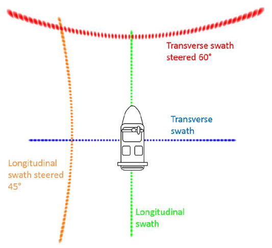
Figure 1: Multiswath capabilities seen from a schematic representation (left): transverse swath footprint is blue, a 60^∘ steered transverse swath is displayed in red, the longitudinal swath is green, and a 45^∘ steered longitudinal swath is orange. Illustration from the operator software (right): An across-track, an along-track, and a tilted along-track swath are observed, as well as an aggregation of fishes and an already constructed bathymetric map.

II-B FLS experiment

The SEAPIX system is being experimented with a Forward-Looking Sonar configuration for predictive target detection and identification. In this context of use, the active face is oriented in the “forward” direction rather than toward the seabed.

In our study, the sensor is installed on the DriX Uncrewed Surface Vehicle (USV), and inclined by 20^∘ according to the pitch angle to the sea surface (Figure 2 left). In transmission, the vertical antenna (formerly longitudinal) generates an enlarged beam of 9^∘ in elevation by 120^∘ in azimuth. A motion stabilized, and electronically tilted firing angle allows the upper limit of the -3 dB transmit beamwidth to graze the sea surface and the lower limit to reach a 50 m depth bottom at about 300 m range. In receive, the horizontal antenna (formerly transverse) generates beams of 2^∘ in azimuth by 120^∘ in elevation and the vertical antenna (which is used again) of 2^∘ in elevation by 120^∘ in azimuth. A rigid sphere of 71 cm diameter (Figure 2 right) is also immersed at 25 m depth in the middle of the water column.

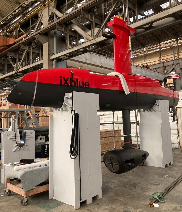
Figure 2: Exail’s DriX USV (left): The cross-shaped linear arrays are visible in the gondola. The real target in open water (right): a metallic sphere of target strength $\displaystyle TS=-15~{}$dB.

So after each transmission of 20 ms Linear Frequency Modulation pulses centered at 150 KHz with a 10 KHz bandwidth and a Pulse Repetition Interval of 0.5 s, the sensor signals from the two antennas are simultaneously recorded, allowing an azimuth and elevation representation of the acoustic environment (Figure 3).

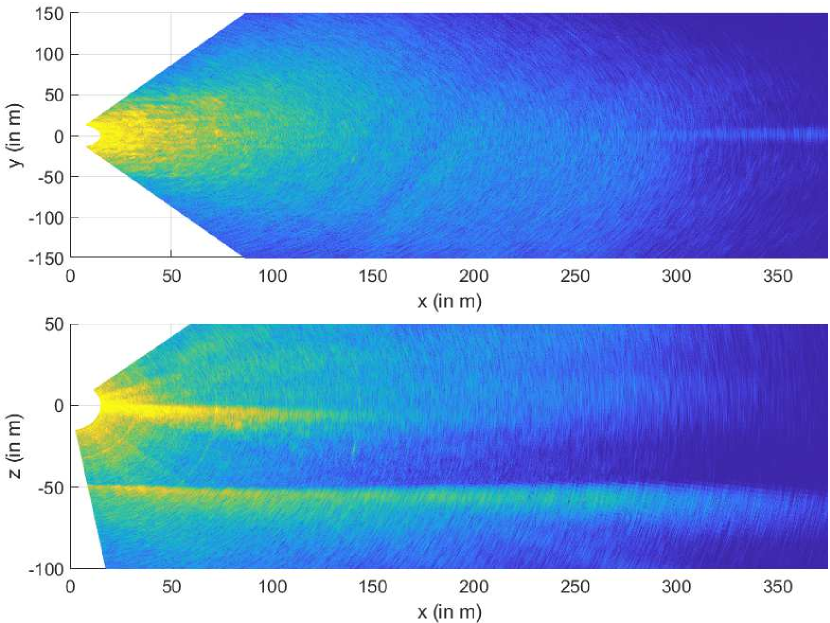
Figure 3: Azimuth (top) and elevation (bottom) view from a single ping, in 50 m depth in La Ciotat bay.

II-C Pre-processing and data format

The signals from the 128 sensors provided by the sonar’s embedded software are demodulated in baseband (In-Phase and Quadrature components) and decimated at 43 KHz. During reception pre-processing, the digitized samples are compensated for the time-varying gain, filtered to the bandwidth of the waveform, pulse compressed, then decimated again to bandwidth.

Finally, a ping dataset is a matrix of about 6000 range bins from 15 m to 400 m, by 64 sensors, by two arrays.

III Detection Schemes

III-A Data model for a single array

At each time, we, have acquired two digitalized synchronized complex data vectors of $\displaystyle m=64$ elements, called “snapshots”, which can be written as (by omitting the temporal parameterization):

$$\mathbf{x}_{i}=\begin{bmatrix}x_{i,1}&x_{i,2}&\cdots&x_{i,m}\end{bmatrix}{}^{T}$$ (1)

where $\displaystyle i=1,2$ is the array identifier (respectively horizontal and vertical).

After the pre-processing steps, a point-like target observed on the antenna $\displaystyle i$ is simply:

$$\mathbf{x}_{i}=\alpha_{i}\,\mathbf{p}_{i}+\mathbf{z}_{i}$$ (2)

where $\displaystyle\mathbf{x}_{i}\in\mathbb{C}^{m}$ is the received signal, $\displaystyle\alpha_{i}$ is an unknown complex target amplitude, $\displaystyle\mathbf{p}_{i}\in\mathbb{C}^{m}$ stands for the known deterministic angular steering vector, $\displaystyle\mathbf{z}_{i}\in\mathbb{C}^{m}$ is a mixture of scaled Gaussian (MSG) random vector admitting the stochastic representation:

$$\mathbf{z}_{i}\overset{d}{=}\sqrt{\tau_{i}}\,\mathbf{c}_{i}.$$ (3)

The texture $\displaystyle\tau_{i}$ is an unknown positive deterministic scalar parameter, presumably different for each range bin (i.e. for all time samples). The speckle $\displaystyle\mathbf{c}_{i}\sim\mathcal{CN}(\mathbf{0},\sigma_{i}^{2}\mathbf{M}_{ii})\in\mathbb{C}^{m}$ is a complex circular Gaussian random vector whose covariance matrix $\displaystyle\mathbf{M}_{ii}$ is known up to a scaling factor $\displaystyle\sigma_{i}^{2}$. The term speckle should be understood in the sense of CES statistics rather than as the result of a sum of contributions from reflections in a resolution cell. This model is strongly related to the class of compound Gaussian distributions [31], which assumes a speckle-independent random texture with a given density $\displaystyle p_{\tau}$. The MSG distribution is more robust than the Gaussian one because the relative scaling between samples allows flexibility in the presence of heterogeneities, such as impulsive noise, outliers, and inconsistent data. This model explicitly allows considering the power fluctuation across range bins, especially for heavy-tailed clutter distributions.

The detection problem is written as a binary hypothesis test:

$$\left\{\begin{array}[]{ll}H_{0}:\mathbf{x}_{i}=\mathbf{z}_{i}&;\quad\mathbf{x}_{i,k}=\mathbf{z}_{i,k}\quad k=1\ldots K\\ H_{1}:\mathbf{x}_{i}=\alpha_{i}\,\mathbf{p}_{i}+\mathbf{z}_{i}&;\quad\mathbf{x}_{i,k}=\mathbf{z}_{i,k}\quad k=1\ldots K.\end{array}\right.\$$ (4)

In (4) it is assumed that $\displaystyle K\geq m$ independent and identically distributed (i.i.d.) signal-free secondary data $\displaystyle\mathbf{x}_{i,k}\in\mathbb{C}^{m}$ are available under both hypotheses for background parameters estimation. We recall that $\displaystyle\mathbf{z}_{i,k}\overset{d}{=}\sqrt{\tau_{i,k}}\,\mathbf{c}_{i,k}$, $\displaystyle\mathbf{c}_{i,k}\sim\mathcal{CN}(\mathbf{0},\mathbf{M}_{ii})$.

Conditionally to the unknown deterministic texture, the densities of $\displaystyle\mathbf{x}_{i}$ under $\displaystyle H_{0}$ and $\displaystyle H_{1}$ are Gaussian:

$$\begin{array}[]{ll}p_{\mathbf{x}_{i}}(\mathbf{x}_{i};H_{0})=\cfrac{1}{\pi^{m}\tilde{\sigma}_{i}^{2m}\lvert\mathbf{M}_{ii}\rvert}\exp\left(-\cfrac{\mathbf{x}_{i}^{H}\mathbf{M}_{ii}^{-1}\mathbf{x}_{i}}{\tilde{\sigma}_{i}^{2}}\right)\,,\\ p_{\mathbf{x}_{i}}(\mathbf{x}_{i};H_{1})=\\ \cfrac{1}{\pi^{m}\tilde{\sigma}_{i}^{2m}\lvert\mathbf{M}_{ii}\rvert}\exp\left(-\cfrac{{\left(\mathbf{x}_{i}-\alpha_{i}\mathbf{p}_{i}\right)}^{H}\mathbf{M}_{ii}^{-1}\left(\mathbf{x}_{i}-\alpha_{i}\mathbf{p}_{i}\right)}{\tilde{\sigma}_{i}^{2}}\right)\,,\end{array}$$ (5)

where $\displaystyle\tilde{\sigma}_{i}=\sigma_{i}\,\sqrt{\tau_{i}}$.

III-B Data model for the two arrays

If we consider the two antennas, this model can be written more appropriately:

$$\left\{\begin{array}[]{ll}H_{0}:\mathbf{x}=\mathbf{z}&;\quad\mathbf{x}_{k}=\mathbf{z}_{k}\quad k=1\ldots K\\ H_{1}:\mathbf{x}=\mathbf{P}\,\boldsymbol{\alpha}+\mathbf{z}&;\quad\mathbf{x}_{k}=\mathbf{z}_{k}\quad k=1\ldots K\end{array}\right.\$$ (6)

where $\displaystyle\mathbf{x}=\begin{bmatrix}\mathbf{x}_{1}\\ \mathbf{x}_{2}\end{bmatrix}\in\mathbb{C}^{2m}$ is the concatenation of the two received signals, $\displaystyle\boldsymbol{\alpha}=\begin{bmatrix}\alpha_{1}\\ \alpha_{2}\end{bmatrix}\in\mathbb{C}^{2}$ is the vector of the target amplitudes and $\displaystyle\mathbf{z}=\begin{bmatrix}\mathbf{z}_{1}\\ \mathbf{z}_{2}\end{bmatrix}\in\mathbb{C}^{2m}$ is the additive clutter. The matrix $\displaystyle\mathbf{P}=\begin{bmatrix}\mathbf{p}_{1}&\mathbf{0}\\ \mathbf{0}&\mathbf{p}_{2}\\ \end{bmatrix}\in\mathbb{C}^{2m\times 2}$ contains the steering vectors. $\displaystyle\left\{\mathbf{x}_{k}=\begin{bmatrix}\mathbf{x}_{1,k}\\ \mathbf{x}_{2,k}\end{bmatrix}\right\}_{k\in[1,K]}\in\mathbb{C}^{2m}$ for $\displaystyle K\geq 2\,m$ are i.i.d. signal-free secondary data.

This formulation allows considering the correlation between sensors of arrays. The covariance is $\displaystyle\mathbf{M}=\begin{bmatrix}\mathbf{M}_{11}&\mathbf{M}_{12}\\ \mathbf{M}_{21}&\mathbf{M}_{22}\end{bmatrix}$, with $\displaystyle\mathbf{M}_{ii}$ the block-covariance matrix of array $\displaystyle i$, and $\displaystyle\mathbf{M}_{ij}=\mathbf{M}_{ji}^{H}$ the cross-correlation block of array $\displaystyle i$ and $\displaystyle j$.

We further assume that the covariance is known, or estimated, up to two scalars, possibly different on each array. These scalars are conditioning the $\displaystyle\mathbf{M}_{ii}$ block-covariance, but also all the cross-correlations blocks associated with the array $\displaystyle i$.

We can therefore write:

$$\widetilde{\mathbf{C}}=\widetilde{\boldsymbol{\Sigma}}\,\mathbf{M}\,\widetilde{\boldsymbol{\Sigma}}\,,$$ (7)

with $\displaystyle\widetilde{\boldsymbol{\Sigma}}=\begin{bmatrix}\tilde{\sigma}_{1}\,\mathbf{I}_{m}&\mathbf{0}\\ \mathbf{0}&\tilde{\sigma}_{2}\,\mathbf{I}_{m}\\ \end{bmatrix}$ = $\displaystyle\begin{bmatrix}\tilde{\sigma}_{1}&0\\ 0&\tilde{\sigma}_{2}\\ \end{bmatrix}\otimes\mathbf{I}_{m}$ the unknown diagonal matrix of scalars $\displaystyle\sigma_{i}$ and $\displaystyle\tau_{i}$. We remind that the $\displaystyle\sigma_{i}$ parameter drives the partial homogeneity of the data (i.e. the difference in scale factor between the covariance matrices of the primary and secondary data) and $\displaystyle\tau_{i}$ drives the non-Gaussianity of the data (i.e. the power variation of the observations over time).

In this model, each array, although correlated, has a possibly distinct texture and an unknown scaling factor on the covariance matrix which may also be dissimilar. It would therefore become entirely possible to model, as an example, a first array whose observations would be Gaussian ($\displaystyle\tau_{1}=1$) and homogeneous ($\displaystyle\sigma_{1}=1$), and a second array whose observations would be K-distributed (for which $\displaystyle\tau_{2}$ is a realization of a Gamma distribution) and non-homogeneous ($\displaystyle\sigma_{2}\neq 1$).

The PDFs under each hypothesis can be rewritten as:

$$\begin{array}[]{ll}p_{\mathbf{x}}(\mathbf{x};H_{0})=\cfrac{1}{\pi^{2m}\lvert\widetilde{\mathbf{C}}\rvert}\exp\left(-{\mathbf{x}}^{H}\widetilde{\mathbf{C}}^{-1}\mathbf{x}\right)\,,\\ p_{\mathbf{x}}(\mathbf{x};H_{1})=\cfrac{1}{\pi^{2m}\lvert\widetilde{\mathbf{C}}\rvert}\exp\left(-{\left(\mathbf{x}-\mathbf{P}\boldsymbol{\alpha}\right)}^{H}\widetilde{\mathbf{C}}^{-1}\left(\mathbf{x}-\mathbf{P}\boldsymbol{\alpha}\right)\right).\end{array}$$ (8)

IV ROBUST DETECTORS

We discuss the derivation of detectors using the GLRT and Rao procedures. Following a two-step approach, the covariance matrix $\displaystyle\mathbf{M}$ will first be assumed known, and then replaced by an appropriate estimator.

IV-A Detectors’ derivation with $\displaystyle\mathbf{M}$ known (step-1)

IV-A1 Generalized Likelihood Ratio Test

The Generalized Likelihood Ratio Test (GLRT) design methodology proposes to solve the detection problem from the ratio of the probability densities function under $\displaystyle H_{1}$ and $\displaystyle H_{0}$, substituting the unknown parameters with their maximum likelihood estimates:

$$L_{G}(\mathbf{x})=\cfrac{\underset{\boldsymbol{\alpha}}{\max}\,\underset{\widetilde{\boldsymbol{\Sigma}}}{\max}\,p_{\mathbf{x}}\left(\mathbf{x};\boldsymbol{\alpha},\widetilde{\boldsymbol{\Sigma}},H_{1}\right)}{\underset{\widetilde{\boldsymbol{\Sigma}}}{\max}\,p_{\mathbf{x}}\left(\mathbf{x};\widetilde{\boldsymbol{\Sigma}},H_{0}\right)}\,.$$ (9)

Proposition IV.1.

The GLRT for the hypothesis test (6) is given by:

$$L_{G}(\mathbf{x})=\cfrac{\hat{\tilde{\sigma}}_{1_{0}}\,\hat{\tilde{\sigma}}_{2_{0}}}{\hat{\tilde{\sigma}}_{1_{1}}\,\hat{\tilde{\sigma}}_{2_{1}}}$$ (10)

where

$$\left(\hat{\tilde{\sigma}}_{1_{0}}\,\hat{\tilde{\sigma}}_{2_{0}}\right)^{2}=\cfrac{\emph{Re}\left(\mathbf{x}_{1}^{H}\mathbf{M}_{12}^{-1}\mathbf{x}_{2}\right)}{m}\\ +\sqrt{\cfrac{\mathbf{x}_{1}^{H}\mathbf{M}_{11}^{-1}\mathbf{x}_{1}}{m}\,\cfrac{\mathbf{x}_{2}^{H}\mathbf{M}_{22}^{-1}\mathbf{x}_{2}}{m}}\,,$$

and

$$\left(\hat{\tilde{\sigma}}_{1_{1}}\,\hat{\tilde{\sigma}}_{2_{1}}\right)^{2}=\cfrac{\emph{Re}\left[\mathbf{x}_{1}^{H}\left(\mathbf{M}_{12}^{-1}-\mathbf{D}_{12}^{-1}\right)\mathbf{x}_{2}\right]}{m}\\ +\sqrt{\cfrac{\mathbf{x}_{1}^{H}\left(\mathbf{M}_{11}^{-1}-\mathbf{D}_{11}^{-1}\right)\mathbf{x}_{1}}{m}\,\cfrac{\mathbf{x}_{2}^{H}\left(\mathbf{M}_{22}^{-1}-\mathbf{D}_{22}^{-1}\right)\mathbf{x}_{2}}{m}}$$

with $\displaystyle\mathbf{D}^{-1}=\mathbf{M}^{-1}\mathbf{P}\left(\mathbf{P}^{H}\mathbf{M}^{-1}\mathbf{P}\right)^{-1}\mathbf{P}^{H}\mathbf{M}^{-1}$.

Proof.

See Appendix A for a step-by-step derivation and Appendix B for some interesting equivalences. ∎

As $\displaystyle\mathbf{x}_{i}=\sqrt{\tau_{i}}\,\mathbf{c}_{i}$ under $\displaystyle H_{0}$, it is easily shown that this detector is texture independent (i.e. it has the texture-CFAR property).

This detection test will be called M-NMF-G in the following.

IV-A2 Rao test

The Rao test is obtained by exploiting the asymptotic efficiency of the ML estimate and expanding the likelihood ratio in the neighborhood of the estimated parameters [47]. A traditional approach for complex unknown parameters is to form a corresponding real-valued parameter vector and then use the real Rao test [48, 49]. Specifically, rewriting the detection problem (6) as:

$$\left\{\begin{array}[]{ll}H_{0}:\boldsymbol{\xi}_{R}=\mathbf{0},\boldsymbol{\xi}_{S}\\ H_{1}:\boldsymbol{\xi}_{R}\neq\mathbf{0},\boldsymbol{\xi}_{S}\,,\end{array}\right.\$$ (11)

where $\displaystyle\boldsymbol{\xi}_{R}=\left[\mathrm{Re}\left(\boldsymbol{\alpha}\right)^{T}\,\mathrm{Im}\left(\boldsymbol{\alpha}\right)^{T}\right]^{T}$ is a $\displaystyle 4\times 1$ parameter vector and $\displaystyle\boldsymbol{\xi}_{S}=\left[\tilde{\sigma}_{1}\,\tilde{\sigma}_{2}\right]^{T}$ is a $\displaystyle 2\times 1$ vector of nuisance parameters, the Rao test for the problem (11) is:

$$L_{R}(\mathbf{x})=\left.\cfrac{\partial\ln p_{\mathbf{x}}(\mathbf{x};\boldsymbol{\xi}_{R},\boldsymbol{\xi}_{S})}{\partial\boldsymbol{\xi}_{R}}\right|_{\begin{matrix}\boldsymbol{\xi}_{R}=\hat{\boldsymbol{\xi}}_{R_{0}}\\ \boldsymbol{\xi}_{S}=\hat{\boldsymbol{\xi}}_{S_{0}}\end{matrix}}^{T}\\ \left[\mathbf{I}^{-1}(\hat{\boldsymbol{\xi}}_{R_{0}},\hat{\boldsymbol{\xi}}_{S_{0}})\right]_{\boldsymbol{\xi}_{R}\boldsymbol{\xi}_{R}}\\ \left.\cfrac{\partial\ln p_{\mathbf{x}}(\mathbf{x};\boldsymbol{\xi}_{R},\boldsymbol{\xi}_{S})}{\partial\boldsymbol{\xi}_{R}}\right|_{\begin{matrix}\boldsymbol{\xi}_{R}=\hat{\boldsymbol{\xi}}_{R_{0}}\\ \boldsymbol{\xi}_{S}=\hat{\boldsymbol{\xi}}_{S_{0}}\end{matrix}}\,.$$ (12)

The PDF $\displaystyle p_{\mathbf{x}}(\mathbf{x};\boldsymbol{\xi}_{R},\boldsymbol{\xi}_{S})$ is given in (8) and parametrized by $\displaystyle\boldsymbol{\xi}_{R}$ and $\displaystyle\boldsymbol{\xi}_{S}$. $\displaystyle\hat{\boldsymbol{\xi}}_{R_{0}}$ and $\displaystyle\hat{\boldsymbol{\xi}}_{S_{0}}$ are the ML estimates of $\displaystyle\boldsymbol{\xi}_{R}$ and $\displaystyle\boldsymbol{\xi}_{S}$ under $\displaystyle H_{0}$. $\displaystyle\mathbf{I}(\boldsymbol{\xi}_{R},\boldsymbol{\xi}_{S})$ is the Fisher Information Matrix that can be partitioned as:

$$\mathbf{I}(\boldsymbol{\xi}_{R},\boldsymbol{\xi}_{S})=\begin{bmatrix}\mathbf{I}_{\boldsymbol{\xi}_{R}\boldsymbol{\xi}_{R}}(\boldsymbol{\xi}_{R},\boldsymbol{\xi}_{S})&\mathbf{I}_{\boldsymbol{\xi}_{R}\boldsymbol{\xi}_{S}}(\boldsymbol{\xi}_{R},\boldsymbol{\xi}_{S})\\ \mathbf{I}_{\boldsymbol{\xi}_{S}\boldsymbol{\xi}_{R}}(\boldsymbol{\xi}_{R},\boldsymbol{\xi}_{S})&\mathbf{I}_{\boldsymbol{\xi}_{S}\boldsymbol{\xi}_{S}}(\boldsymbol{\xi}_{R},\boldsymbol{\xi}_{S})\end{bmatrix}\,,$$

and we have:

$$\left[\mathbf{I}^{-1}(\boldsymbol{\xi}_{R},\boldsymbol{\xi}_{S})\right]_{\boldsymbol{\xi}_{R}\boldsymbol{\xi}_{R}}=\left(\mathbf{I}_{\boldsymbol{\xi}_{R}\boldsymbol{\xi}_{R}}(\boldsymbol{\xi}_{R},\boldsymbol{\xi}_{S})-\right.\\ \left.\mathbf{I}_{\boldsymbol{\xi}_{R}\boldsymbol{\xi}_{S}}(\boldsymbol{\xi}_{R},\boldsymbol{\xi}_{S})\,\mathbf{I}_{\boldsymbol{\xi}_{S}\boldsymbol{\xi}_{S}}^{-1}(\boldsymbol{\xi}_{R},\boldsymbol{\xi}_{S})\,\mathbf{I}_{\boldsymbol{\xi}_{S}\boldsymbol{\xi}_{R}}(\boldsymbol{\xi}_{R},\boldsymbol{\xi}_{S})\right)^{-1}\,.$$ (13)

The following proposition can be finally stated:

Proposition IV.2.

The Rao test is given by:

$$L_{R}(\mathbf{x})=2\,\mathbf{x}^{H}\hat{\widetilde{\mathbf{C}}}_{0}^{-1}\mathbf{P}\left(\mathbf{P}^{H}\hat{\widetilde{\mathbf{C}}}_{0}^{-1}\mathbf{P}\right)^{-1}\mathbf{P}^{H}\hat{\widetilde{\mathbf{C}}}_{0}^{-1}\mathbf{x}$$ (14)

where $\displaystyle\hat{\widetilde{\mathbf{C}}}_{0}=\hat{\widetilde{\boldsymbol{\Sigma}}}_{0}\,\mathbf{M}\,\hat{\widetilde{\boldsymbol{\Sigma}}}_{0}$ and $\displaystyle\hat{\widetilde{\boldsymbol{\Sigma}}}_{0}$ is defined in Appendix A.

Proof.

See Appendix C. ∎

As for the GLRT, (14) is texture-CFAR. This detector will be referred to as M-NMF-R in the sequel.

IV-B Covariance estimation and adaptive detectors (step-2)

In practice, the noise covariance matrix is unknown and estimated using the $\displaystyle K$ available i.i.d. signal-free secondary data.

In Gaussian environment, in which PDFs are given by (8) with $\displaystyle\sigma_{i}=1$ and $\displaystyle\tau_{i}=1$, the MLE of $\displaystyle\mathbf{M}$ is the well-known Sample Covariance Matrix (SCM):

$$\widehat{\mathbf{M}}_{SCM}=\cfrac{1}{K}\sum_{k=1}^{K}\mathbf{x}_{k}\mathbf{x}_{k}^{H}$$ (15)

which is an unbiased and minimum variance estimator.

In the presence of outliers or a heavy-tailed distribution (as modeled by a mixture of scaled Gaussian), this estimator is no longer optimal or robust. This leads to a strong performance degradation.

Proposition IV.3.

In MSG environment the MLE of $\displaystyle\mathbf{M}$ is given by:

$$\widehat{\mathbf{M}}_{\text{2TYL}}=\cfrac{1}{K}\sum_{k=1}^{K}\widehat{\mathbf{T}}_{k}^{-1}\mathbf{x}_{k}\mathbf{x}_{k}^{H}\widehat{\mathbf{T}}_{k}^{-1}\,,$$ (16)

where $\displaystyle\widehat{\mathbf{T}}_{k}=\begin{bmatrix}\sqrt{\hat{\tau}_{1_{k}}}&0\\ 0&\sqrt{\hat{\tau}_{2_{k}}}\\ \end{bmatrix}\otimes\mathbf{I}_{m}$, $\displaystyle\hat{\tau}_{1_{k}}=t_{1}+\sqrt{\cfrac{t_{1}}{t_{2}}}\,t_{12}$, $\displaystyle\hat{\tau}_{2_{k}}=t_{2}+\sqrt{\cfrac{t_{2}}{t_{1}}}\,t_{12}$ and $\displaystyle t_{1}=\cfrac{\mathbf{x}_{1,k}^{H}\widehat{\mathbf{M}}_{11}^{-1}\mathbf{x}_{1,k}}{m}$, $\displaystyle t_{2}=\cfrac{\mathbf{x}_{2,k}^{H}\widehat{\mathbf{M}}_{22}^{-1}\mathbf{x}_{2,k}}{m}$, $\displaystyle t_{12}=\cfrac{\text{Re}\left(\mathbf{x}_{1,k}^{H}\widehat{\mathbf{M}}_{12}^{-1}\mathbf{x}_{2,k}\right)}{m}$.

Proof.

The demonstration is provided in Appendix D. ∎

A key point is that this estimator is independent of the textures, i.e. the power variations, on each array. It can be thought of as a multi-texture generalization of [38].

From a practical point of view $\displaystyle\widehat{\mathbf{M}}_{\text{2TYL}}$ is the solution of the recursive algorithm:

$$\displaystyle\widehat{\mathbf{T}}_{k}^{(n)} \displaystyle=\begin{bmatrix}\sqrt{\hat{\tau}_{1_{k}}^{(n)}}&0\\ 0&\sqrt{\hat{\tau}_{2_{k}}^{(n)}}\\ \end{bmatrix}\otimes\mathbf{I}_{m}\,,$$ (17)

$$\displaystyle\widehat{\mathbf{M}}_{\text{2TYL}}^{(n)} \displaystyle=\cfrac{1}{K}\sum_{k=1}^{K}\left(\widehat{\mathbf{T}}_{k}^{(n-1)}\right)^{-1}\mathbf{x}_{k}\mathbf{x}_{k}^{H}\left(\widehat{\mathbf{T}}_{k}^{(n-1)}\right)^{-1}\,,$$ (18)

where $\displaystyle n\in\mathbb{N}$ is the iteration number, whatever the initialization $\displaystyle\widehat{\mathbf{M}}_{\text{2TYL}}^{(0)}$.

The convergence of recursive equations (17) and (18) in the estimation of $\displaystyle\widehat{\mathbf{M}}_{\text{2TYL}}$ is illustrated in Figure 4 for 500 iterations and $\displaystyle\widehat{\mathbf{M}}_{\text{2TYL}}^{(0)}=\mathbf{I}_{2m}$.

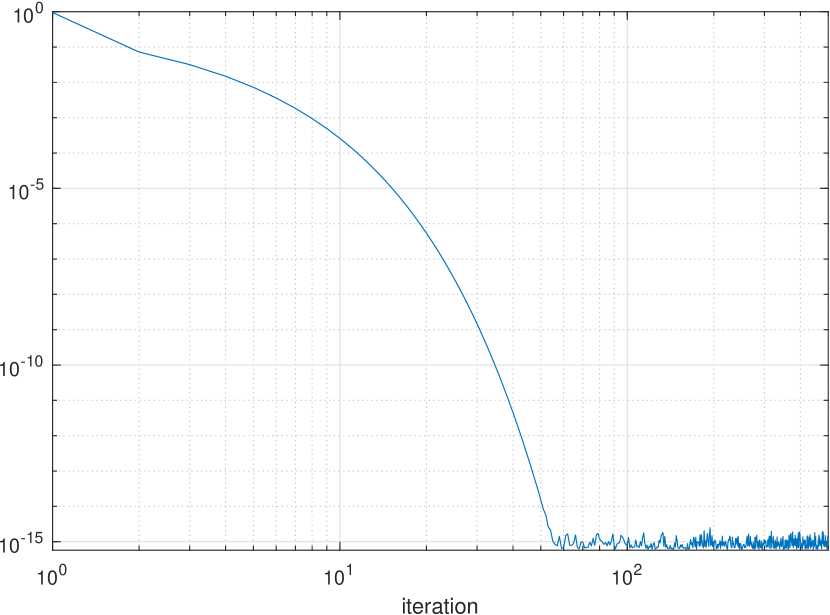
Figure 4: Relative deviations of the estimates as a function of the number of iterations ($\displaystyle\widehat{\mathbf{M}}_{\text{2TYL}}^{(0)}=\mathbf{I}_{2m}$).

The relative difference between estimates decreases with the number of iterations. From iteration 60, the accuracy becomes limited by the simulation environment. In practice, it is not necessary to go to this limit, and we notice that from iteration 20 the relative deviation becomes lower than $\displaystyle 10^{-6}$.

At last, the adaptive versions of the tests (10) and (14) will be simply obtained by replacing the covariance matrix $\displaystyle\mathbf{M}$ by an appropriate estimate: (15) or (16) according to the environment. Those detectors will be referred as M-ANMF-G_SCM, M-ANMF-R_SCM, M-ANMF-G_TYL, and M-ANMF-R_TYL.

V Numerical results on simulated data

V-A Performance assessment

Two correlation coefficients $\displaystyle\rho_{1}$ and $\displaystyle\rho_{2}$ $\displaystyle\left(0<\rho_{1},\rho_{2}<1\right)$, are used in the construction of a speckle covariance matrix model defined as:

$$\left[\mathbf{M}\right]_{jl}=\beta\,\rho_{1}^{\lvert j_{1}-l_{1}\rvert}\times\rho_{2}^{\lvert j_{2}-l_{2}\rvert}\,,$$

where $\displaystyle j,l\in\left[1,\,2m\right]$ are sensor numbers of coordinates $\displaystyle\left(j_{1},j_{2}\right)$ and $\displaystyle\left(l_{1},l_{2}\right)$ respectively and $\displaystyle\beta$ is a scale factor. Thus, denoting $\displaystyle\mathbf{M}=\begin{bmatrix}\mathbf{M}_{11}&\mathbf{M}_{12}\\ \mathbf{M}_{21}&\mathbf{M}_{22}\end{bmatrix}$, $\displaystyle\mathbf{M}_{11}$ and $\displaystyle\mathbf{M}_{22}$ are the covariance matrices of array 1 and 2 and $\displaystyle\mathbf{M}_{12}=\mathbf{M}_{21}^{H}$ is a cross-correlation block. In the FLS context, the block $\displaystyle\mathbf{M}_{11}$ is weakly correlated and Toeplitz structured (close to the identity matrix). $\displaystyle\mathbf{M}_{22}$ is also Toeplitz but more strongly correlated (due to the wider transmission beam). The cross-correlation blocks could be considered null under the uncorrelated arrays assumption. In our case, these will be different from zero because the arrays cross each other in their central part. This results in the general structure displayed in Figure 5, where we visually show the adequacy of this model with the SCM covariance estimator established on real data.

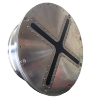
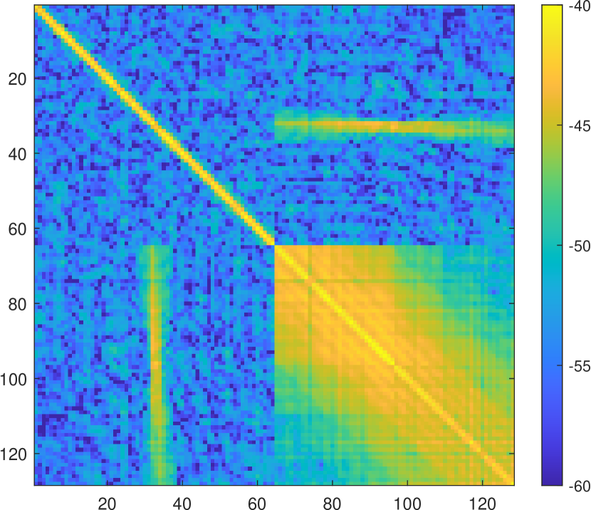
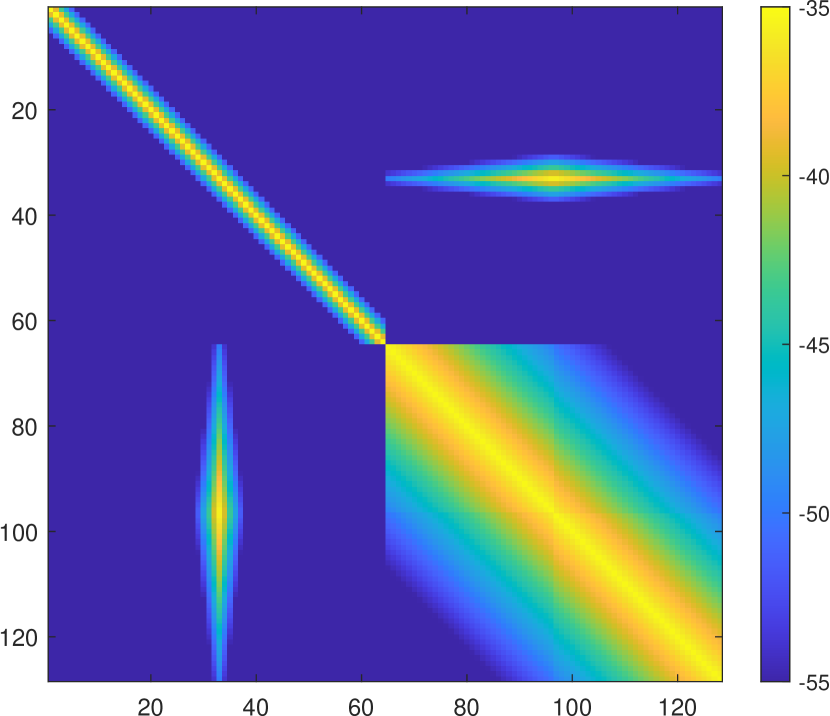
Figure 5: Sonar arrays (left): two uniform linear arrays intersect in their centers. Empirical covariance matrix on real sonar data shown in dB (center): The SCM is estimated on a homogeneous area between 265 m and 328 m. Cross-correlation blocks are non-zero. The covariance matrix model used for the data simulation is shown in dB (right): $\displaystyle\beta=3\times 10^{-4}$, $\displaystyle\rho_{1}=0.4$, $\displaystyle\rho_{2}=0.9$.

We choose $\displaystyle\sigma_{i}=1$. $\displaystyle\tau_{i}=1$ for Gaussian clutter and $\displaystyle\tau_{i}\sim\mathrm{Gam}(\nu,1/\nu)$ with $\displaystyle\nu=0.5$ for impulsive non-Gaussian K-distributed data (that is, the texture variables follow a gamma distribution with shape parameter 0.5 and scale parameter 2). The PFA-threshold curves are established on the basis of 1000 realizations of random vectors. The detection probabilities are statistically estimated by adding a synthetic narrow band far field point target with identical amplitudes on the arrays ($\displaystyle\alpha_{1}=\alpha_{2}$). 10000 Monte Carlo iterations are performed and 150 target amplitudes are evaluated.

V-B Benchmark tests

The GLRT for a single array in a partially homogeneous Gaussian environment when $\displaystyle\mathbf{M}_{ii}$ is known is the Normalized Matched Filter [11]:

$$\text{NMF}i(\mathbf{x}_{i})=\cfrac{\lvert\mathbf{p}_{i}^{H}\mathbf{M}_{ii}^{-1}\mathbf{x}_{i}\rvert^{2}}{\left(\mathbf{p}_{i}^{H}\mathbf{M}_{ii}^{-1}\mathbf{p}_{i}\right)\left(\mathbf{x}_{i}^{H}\mathbf{M}_{ii}^{-1}\mathbf{x}_{i}\right)}\,.$$ (19)

Adaptive versions are obtained by substituting the covariance matrix by a suitable estimate [35] and will be referred to as ANMF${}_{SCM}i$ in Gaussian case, or ANMF${}_{TYL}i$ for the non-Gaussian case.

When the two arrays are considered, in the very favorable case of a Gaussian homogeneous environment where the covariance matrix $\displaystyle\mathbf{C}$ is perfectly known, the GLRT is:

$$\text{MIMO-MF}(\mathbf{x})=\mathbf{x}^{H}\mathbf{C}^{-1}\mathbf{P}\left(\mathbf{P}^{H}\mathbf{C}^{-1}\mathbf{P}\right)^{-1}\mathbf{P}^{H}\mathbf{C}^{-1}\mathbf{x}\,.$$ (20)

This is the MIMO Optimum Gaussian Detector (R-MIMO OGD) in [50], which is a multi-array generalization of the Matched Filter test. One can note the very strong similarity with (14). Its adaptive version is MIMO-AMF_SCM. It seems useful to specify that this detector is relevant only in a Gaussian and perfectly homogeneous environment. Especially, exactly as in the single-array case [31], the covariance estimator (16) is defined up to a constant scalar. Detectors (10) and (14) are invariant when the covariance is changed by a scale factor. This is a direct result of the partial homogeneity assumption. This is not the case for (20), thus the adaptive MIMO-AMF_TYL version is not relevant and will not be used in the following.

These tests will be considered as performance bounds for the proposed detectors: M-NMF-G and M-NMF-R when $\displaystyle\mathbf{M}$ is known, M-ANMF-G_SCM, M-ANMF-R_SCM, M-ANMF-G_TYL and M-ANMF-R_TYL otherwise.

V-C Performance in Gaussian clutter

We have showed that all developed detectors are texture-CFAR. Unfortunately, the matrix CFAR property (distribution of the test keeps identical whatever the true covariance matrix) is much more difficult to show. Therefore, we propose to perform a study on simulated data to check this matrix CFAR property. Figure 6 experimentally demonstrates the CFAR behavior of the detectors with respect to the covariance matrix in a Gaussian environment. On the left side we represent the false alarm probability of Rao’s detector (for known and estimated $\displaystyle\mathbf{M}$) as a function of the detection threshold. On the right, these curves are plotted for the GLRT detector.

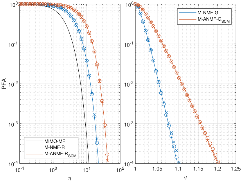
Figure 6: Pfa-threshold curves of the M-(A)NMF-R_SCM and M-(A)NMF-G_SCM detectors in Gaussian environment. Left: the Rao detector for known $\displaystyle\mathbf{M}$ (blue), for $\displaystyle\mathbf{M}$ estimated from $\displaystyle 2\times 2m$ secondary data (red), the OGD detector or Matched Filter (black). Right: The GLRT detector for known $\displaystyle\mathbf{M}$ (blue), and estimated based on $\displaystyle 2\times 2m$ secondary data (red).

The deviation of the adaptive detectors comes from the covariance estimation process: the red curve converges to the blue one when the number of secondary data used for the estimation of $\displaystyle\mathbf{M}$ increases.

The markers represent curves for different covariances. In solid line $\displaystyle\beta=3\times 10^{-4}$, $\displaystyle\rho_{1}=0.4$, $\displaystyle\rho_{2}=0.9$. The cross markers are established from $\displaystyle\beta=1$, $\displaystyle\rho_{1}=0.95$, $\displaystyle\rho_{2}=0.95$. Circular markers are for $\displaystyle\beta=100$, $\displaystyle\rho_{1}=0.1$, $\displaystyle\rho_{2}=0.1$ and null anti-diagonal blocks. For very distinct covariances, the superposition of curves and markers underlines the matrix-CFAR property of the detectors.

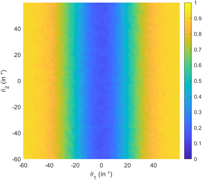
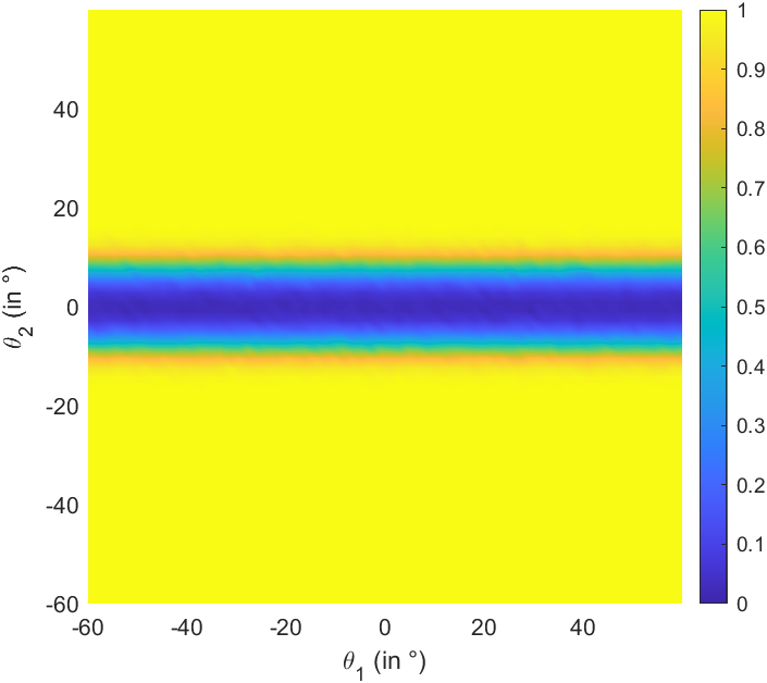
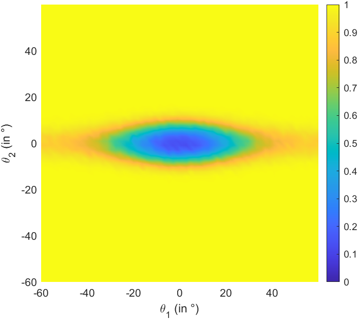
Figure 7: Probability of detection in Gaussian environment for known covariance matrix $\displaystyle\mathbf{M}$ as a function of $\displaystyle\theta_{1}$ and $\displaystyle\theta_{2}$ ($\displaystyle\beta=3\times 10^{-4}$, $\displaystyle\rho_{1}=0.4$, $\displaystyle\rho_{2}=0.9$, $\displaystyle SNR=-12~{}$dB and $\displaystyle PFA=10^{-2}$). Top left: NMF 1. Top right: NMF 2. Bottom left: M-NMF-R.

Figure 7 illustrates the value of merging arrays with a cross-shaped geometry. The detection probabilities of NMF 1, NMF 2, and M-NMF-R are plotted as a function of azimuth ($\displaystyle\theta_{1}$) and elevation ($\displaystyle\theta_{2}$) angles at fixed SNR.

In the first angular dimension, which depends on the array considered, each ULA has a zone of least detectability close to 0^∘. This is due to the correlated nature of clutter. The decrease in detection probabilities from +/-60^∘ to 0^∘ is a function of the correlation level ($\displaystyle\rho_{1}$ or $\displaystyle\rho_{2}$). In the second dimension, the detection performances are invariant. Thus, the poor detection performance near 0^∘ propagates in a whole direction of space: “vertically” for NMF 1 and “horizontally” for NMF 2. As an illustration, the probability of detection of NMF 1 in $\displaystyle\theta_{1}=0^{\circ}$ whatever $\displaystyle\theta_{2}$ is $\displaystyle PD=0.17$, and the probability of detection of NMF 2 in $\displaystyle\theta_{2}=0^{\circ}$ for all $\displaystyle\theta_{1}$ is 0.03.

The M-NMF-R detector spatially minimizes this area of least detectability. In this case, the probability of detection at $\displaystyle\theta_{1}=0^{\circ}$ becomes greater than $\displaystyle 0.8$ for $\displaystyle\lvert\theta_{2}\rvert>10.5^{\circ}$ and greater than $\displaystyle 0.5$ for $\displaystyle\theta_{2}=0^{\circ}$ and $\displaystyle\lvert\theta_{1}\rvert>24^{\circ}$. The Rigde clutter is minimized.

The probability of detection (PD) is plotted as a function of the signal-to-noise ratio (SNR) in Figure 8 when $\displaystyle\mathbf{M}$ is known.

\begin{overpic}[width=433.62pt]{pd_snr_G_distrib_M_known_resized.pdf} \put(12.0,43.0){\includegraphics[width=190.79385pt]{pd_snr_G_distrib_M_known_zoom_resized.pdf}} \end{overpic}

Figure 8: Probability of detection in Gaussian environment for known $\displaystyle\mathbf{M}$ ($\displaystyle\beta=3\times 10^{-4}$, $\displaystyle\rho_{1}=0.4$, $\displaystyle\rho_{2}=0.9$ and $\displaystyle PFA=10^{-2}$).

The MIMO-MF detector (shown in black), which requires a perfect knowledge of the covariance, is logically the most efficient. The single array NMF detectors (NMF 1 and 2, in purple and green) have comparable and the lowest performance. The M-NMF-I detector (in blue) between these curves assumes antenna independence. The proposed M-NMF-G (red) and M-NMF-R (yellow) detectors are both equivalent and superior to the M-NMF-I (0.2 dB at $\displaystyle PD=0.8$) and much more efficient than NMF 1 (2.5 dB) and NMF 2 tests (2 dB). The difference with MIMO-MF is slight, around 0.2 dB at $\displaystyle PD=0.8$. Detection performances by the Rao approach are slightly superior to those obtained by the GLRT.

Figure 9 compares the performance of the tests in their adaptive versions. The MIMO-MF curve is shown in black dotted lines for illustrative purposes only (as it assumes the covariance known). It can be seen that when the SCM is evaluated on $\displaystyle 2\times 2m=256$ secondary data, the covariance estimation leads to a loss of 3 dB between the performances of the MIMO-MF test and its adaptive version MIMO-AMF, as expected from the Reed-Mallett-Brennan’s rule [51].

\begin{overpic}[width=433.62pt]{pd_snr_G_distrib_M_unknown_resized.pdf} \put(12.0,43.0){\includegraphics[width=190.79385pt]{pd_snr_G_distrib_M_unknown_zoom_resized.pdf}} \end{overpic}

Figure 9: Probability of detection in Gaussian environment for unknown $\displaystyle\mathbf{M}$ ($\displaystyle PFA=10^{-2}$, SCMs are estimated based on $\displaystyle 2\times 2m$ secondary data).

In their adaptive versions, the proposed detectors offer equivalent performances to the MIMO-AMF detectors while offering additional robustness and flexibility conditions on a possible lack of knowledge of the covariance (estimated to be within two scale factors). The gain compared to single array detectors, although reduced compared to the case where $\displaystyle\mathbf{M}$ is known, remains favorable and of the order of 0.5 to 1 dB at $\displaystyle PD=0.8$. In other words, for an SNR of -11 dB, $\displaystyle PD=0.75$ for ANMF 1 and 0.85 for M-ANMF-G_SCM (or M-ANMF-R_SCM).

V-D Performance in impulsive non-Gaussian clutter

PFA-threshold curves in K-distributed environment are displayed in Figure 10 in order to characterize the matrix-CFAR behavior.

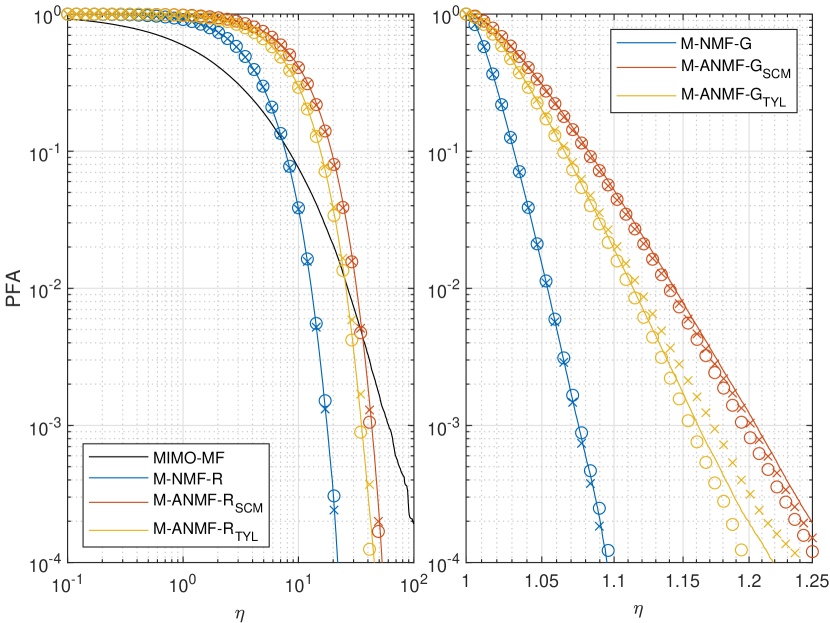
Figure 10: Pfa-threshold curves in non-Gaussian K-distributed environment ($\displaystyle\nu=0.5$). Left: the Rao detector for known $\displaystyle\mathbf{M}$ (blue), for $\displaystyle\mathbf{M}$ estimated with the SCM (red), $\displaystyle\mathbf{M}$ estimated with the new estimator (yellow), the OGD detector or Matched Filter (black). Right: The GLRT detector for known $\displaystyle\mathbf{M}$ (blue), $\displaystyle\mathbf{M}$ estimated based on the SCM (red), based on Tyler’s extension (yellow).

The detectors based on the new covariance matrix estimator systematically have lower detection thresholds to those obtained with the SCM. While optimal for a Gaussian clutter, the MIMO-MF detector is no longer suitable. The marker overlays highlight the matrix-CFAR behavior of the Rao detector in a non-Gaussian environment. The case of the GLRT detector is much less obvious: at this stage, it seems complicated to consider that the false alarm curves are strictly independent of the covariance matrix.

The detection performances are compared in Figure 11.

\begin{overpic}[width=433.62pt]{pd_snr_K05_distrib_M_unknown_resized.pdf} \put(12.0,43.0){\includegraphics[width=190.79385pt]{pd_snr_K05_distrib_M_unknown_zoom_resized.pdf}} \end{overpic}

Figure 11: Probability of detection in K-distributed environment for unknown $\displaystyle\mathbf{M}$ ($\displaystyle\nu=0.5$, $\displaystyle PFA=10^{-2}$, $\displaystyle 2\times 2m$ secondary data). In solid lines, the detectors are built with the SCM estimate. In dotted lines, the detectors are built with Tyler’s (single array) or the new (dual arrays) estimator.

For the Rao and GLRT detectors, using the estimator (16) in an impulsive non-Gaussian environment induces a gain in detection performance of the order of 1.2 dB at $\displaystyle PD=0.8$ with the SCM. Compared to the best competitors the improvement is 3 dB at $\displaystyle PD=0.8$.

VI Experimental data with real target

The actual sonar measurements were collected during an acquisition campaign in May 2022 in La Ciotat bay, Mediterranean Sea. The experimental conditions are described in II-B, and the dataset of interest is shown in Figure 3. Echoes from the true target (right in Figure 2 ) are observed at the 2040th range cell.

VI-A Illustrations of detection test outputs

Figure 12 provides examples of real data outputs from conventional ANMF detectors based on a single array. The real target is observed in range bin 2040 (143 m away from the sonar), at angular bin $\displaystyle\theta_{1}=26$ ($\displaystyle-12.4^{\circ}$ azimuth), and angular bin $\displaystyle\theta_{2}=37$ ($\displaystyle 8.6^{\circ}$ elevation).

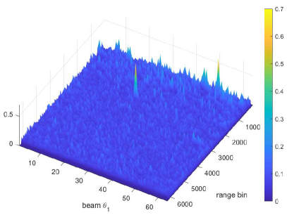
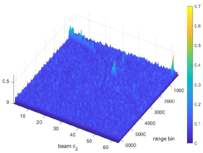
Figure 12: ANMF_SCM detector outputs on real sonar data. A target is observed on array 1 (left) at coordinates $\displaystyle(26,\,2040)$ and on array 2 (right) at coordinates $\displaystyle(37,\,2040)$. The SCM is built from 256 secondary data.

Figure 13 shows the outputs of the Rao and GLRT detectors applied simultaneously to both arrays at the specific range bin 2040. These subfigures are not directly comparable with each other or with Figure 12. The target is perfectly located in azimuth and elevation.

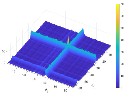
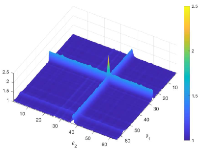
Figure 13: Outputs of the M-ANMF-R_SCM (left) and M-ANMF-G_SCM (right) detectors. The real target is at coordinates (37,  26). The SCM is built from 256 secondary data.

VI-B Robustness to training data corruption

Previously, we assumed the availability of a set of $\displaystyle K\geq 2m$ i.i.d. secondary data, supposed free of signal components and sharing statistic properties with the noise in the cell under test. In practice, such data can be obtained by processing samples in spatial proximity to the range bin being evaluated, and the absence of signals is not always verified or checkable. In particular, this assumption is no longer valid if another target is present in these secondary data.

Figure 14 illustrates the robustness of the covariance matrix estimators to data corruption. A synthetic target is added 100 samples away from the real target and contaminates the secondary dataset.

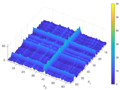
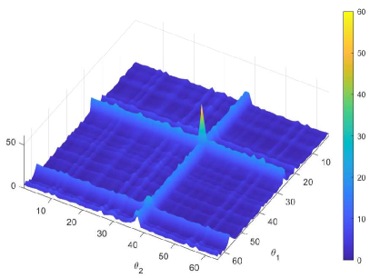
Figure 14: Rao detector outputs based on the SCM (left) or Tyler (right) with secondary data corruption. The covariance matrix estimators are based on 256 secondary data.

On the left side, the output of M-ANMF-R_SCM is strongly degraded. The SCM is not robust to the presence of outliers. The target is hardly discernible, and the maximum is wrongly located.

Under the same conditions, the response of the M-ANMF-R_TYL detector is visualized in the right part. Although degraded compared to Figure 13, the behavior is still largely usable. The target presence is easily identified, and the new estimator (16) is much more resistant to data contamination.

VII Conclusions

In this paper, we considered the problem of adaptive point target detection by a correlated multi-arrays Mills Cross sonar system. Using a 2-step approach, we first derived two new detectors that are robust to differences in target amplitudes and to unknown scaling factors on the covariances. Subsequently, we have introduced an innovative estimator of the covariance matrix suitable to any non-Gaussian MSG environment. By these very general assumptions, the framework of the study can therefore concern systems with co-located or remote arrays.

Experimental results show that the detection performance is up to 3 dB better than conventional approaches. The detectors cover a larger detection area and are particularly robust to spikes, impulsive noise, and data contamination.

Future work will focus on establishing a theoretical demonstration of the matrix-CFAR behavior of these detectors, and on generalizing solutions for different numbers and geometries of arrays.

Appendix A GLRT’s derivation

For the following, and for ease of reading, the punctuation mark “tilde” will be omitted. Thus $\displaystyle\widetilde{\Sigma}$ and $\displaystyle\tilde{\sigma}_{i}$ will simply be denoted as $\displaystyle\Sigma$ and $\displaystyle\sigma_{i}$. The same is true for their respective estimates.

A-A Maximum Likelihood Estimator of $\displaystyle\boldsymbol{\Sigma}$ under $\displaystyle H_{0}$

The MLE $\displaystyle\hat{\boldsymbol{\Sigma}}_{0}$ is derived from the log-likelihood function:

$$\begin{array}[]{ll}\ln p_{\mathbf{x}}(\mathbf{x};\boldsymbol{\Sigma},H_{0})=\\ -mL\ln\pi+2\ln\lvert\boldsymbol{\Sigma}^{-1}\rvert-\ln\lvert\mathbf{M}\rvert-\left({\mathbf{x}}^{H}\boldsymbol{\Sigma}^{-1}\mathbf{M}^{-1}\boldsymbol{\Sigma}^{-1}\mathbf{x}\right)\,,\end{array}$$

whose derivative relative to $\displaystyle\boldsymbol{\Sigma}^{-1}$ is:

$$\cfrac{\partial\ln p_{\mathbf{x}}(\mathbf{x};\boldsymbol{\Sigma},H_{0})}{\partial\boldsymbol{\Sigma}^{-1}}=2\cfrac{\partial\ln\lvert\boldsymbol{\Sigma}^{-1}\rvert}{\partial\boldsymbol{\Sigma}^{-1}}-\cfrac{\partial\mathbf{x}^{H}\boldsymbol{\Sigma}^{-1}\mathbf{M}^{-1}\boldsymbol{\Sigma}^{-1}\mathbf{x}}{\partial\boldsymbol{\Sigma}^{-1}}\,.$$

Knowing that ([52] (57)) $\displaystyle\cfrac{\partial\ln\lvert\boldsymbol{\Sigma}^{-1}\rvert}{\partial\boldsymbol{\Sigma}^{-1}}=\boldsymbol{\Sigma}$, and ([52] (82)) $\displaystyle\cfrac{\partial\mathbf{x}^{H}\boldsymbol{\Sigma}^{-1}\mathbf{M}^{-1}\boldsymbol{\Sigma}^{-1}\mathbf{x}}{\partial\boldsymbol{\Sigma}^{-1}}=2\text{Re}\left(\mathbf{M}^{-1}\boldsymbol{\Sigma}^{-1}\mathbf{x}\,\mathbf{x}^{H}\right)$ we have:

$$\cfrac{\partial\ln p_{\mathbf{x}}(\mathbf{x};\boldsymbol{\Sigma},H_{0})}{\partial\boldsymbol{\Sigma}^{-1}}=2\boldsymbol{\Sigma}-2\text{Re}\left(\mathbf{M}^{-1}\boldsymbol{\Sigma}^{-1}\mathbf{x}\,\mathbf{x}^{H}\right)\,,$$

which leads to:

$$\hat{\boldsymbol{\Sigma}}_{0}=\text{Re}\left(\mathbf{M}^{-1}\hat{\boldsymbol{\Sigma}}_{0}^{-1}\mathbf{x}\,\mathbf{x}^{H}\right)\,.$$ (21)

Expanding this matrix product with $\displaystyle\hat{\boldsymbol{\Sigma}}_{0}=\begin{bmatrix}\hat{\sigma}_{1_{0}}\mathbf{I}_{m}&\mathbf{0}\\ \mathbf{0}&\hat{\sigma}_{2_{0}}\mathbf{I}_{m}\\ \end{bmatrix}$, we have:

$$\hat{\sigma}_{1_{0}}\,\mathbf{I}_{m}=\text{Re}\left(\mathbf{M}_{11}^{-1}\cfrac{\mathbf{x}_{1}\,\mathbf{x}_{1}^{H}}{\hat{\sigma}_{1_{0}}}+\mathbf{M}_{12}^{-1}\cfrac{\mathbf{x}_{2}\,\mathbf{x}_{1}^{H}}{\hat{\sigma}_{2_{0}}}\right)\,,$$

and using the trace operator:

$$\displaystyle m\,\hat{\sigma}_{1_{0}} \displaystyle=\operatorname{tr}\left[\text{Re}\left(\mathbf{M}_{11}^{-1}\cfrac{\mathbf{x}_{1}\,\mathbf{x}_{1}^{H}}{\hat{\sigma}_{1_{0}}}+\mathbf{M}_{12}^{-1}\cfrac{\mathbf{x}_{2}\,\mathbf{x}_{1}^{H}}{\hat{\sigma}_{2_{0}}}\right)\right]$$

$$\displaystyle=\cfrac{\mathbf{x}_{1}^{H}\mathbf{M}_{11}^{-1}\mathbf{x}_{1}}{\hat{\sigma}_{1_{0}}}+\text{Re}\left(\cfrac{\mathbf{x}_{1}^{H}\mathbf{M}_{12}^{-1}\mathbf{x}_{2}}{\hat{\sigma}_{2_{0}}}\right)\,.$$

We then have:

$$\hat{\sigma}_{1_{0}}=\cfrac{1}{\hat{\sigma}_{1_{0}}}\cfrac{\mathbf{x}_{1}^{H}\mathbf{M}_{11}^{-1}\mathbf{x}_{1}}{m}+\cfrac{1}{\hat{\sigma}_{2_{0}}}\cfrac{\text{Re}\left(\mathbf{x}_{1}^{H}\mathbf{M}_{12}^{-1}\mathbf{x}_{2}\right)}{m}\,,$$ (22)

and

$$\hat{\sigma}_{2_{0}}=\cfrac{1}{\hat{\sigma}_{1_{0}}}\cfrac{\text{Re}\left(\mathbf{x}_{2}^{H}\mathbf{M}_{21}^{-1}\mathbf{x}_{1}\right)}{m}+\cfrac{1}{\hat{\sigma}_{2_{0}}}\cfrac{\mathbf{x}_{2}^{H}\mathbf{M}_{22}^{-1}\mathbf{x}_{2}}{m}\,.$$ (23)

Denoting $\displaystyle a_{1}=\cfrac{\mathbf{x}_{1}^{H}\mathbf{M}_{11}^{-1}\mathbf{x}_{1}}{m}$, $\displaystyle a_{12}=\cfrac{\text{Re}\left(\mathbf{x}_{1}^{H}\mathbf{M}_{12}^{-1}\mathbf{x}_{2}\right)}{m}$,
$\displaystyle a_{2}=\cfrac{\mathbf{x}_{2}^{H}\mathbf{M}_{22}^{-1}\mathbf{x}_{2}}{m}$ and using (22) and (23):

$$\left\{\begin{array}[]{ll}\hat{\sigma}_{1_{0}}^{2}=a_{1}+\cfrac{\hat{\sigma}_{1_{0}}}{\hat{\sigma}_{2_{0}}}\,a_{12}\\ \hat{\sigma}_{2_{0}}^{2}=\cfrac{\hat{\sigma}_{2_{0}}}{\hat{\sigma}_{1_{0}}}\,a_{12}+a_{2}\,,\end{array}\right.\$$ (24)

or:

$$\left\{\begin{array}[]{ll}\hat{\sigma}_{1_{0}}^{2}=a_{1}+\cfrac{\hat{\sigma}_{1_{0}}}{\hat{\sigma}_{2_{0}}}\,a_{12}\\ \hat{\sigma}_{1_{0}}^{2}=\cfrac{\hat{\sigma}_{1_{0}}}{\hat{\sigma}_{2_{0}}}\,a_{12}+\cfrac{\hat{\sigma}_{1_{0}}^{2}}{\hat{\sigma}_{2_{0}}^{2}}\,a_{2}\,.\end{array}\right.\$$

By equalization of right-hand terms:

$$a_{1}=\cfrac{\hat{\sigma}_{1_{0}}^{2}}{\hat{\sigma}_{2_{0}}^{2}}\,a_{2}\,,$$

and keeping the positive solution: $\displaystyle\cfrac{\hat{\sigma}_{1_{0}}}{\hat{\sigma}_{2_{0}}}=\sqrt{\cfrac{a_{1}}{a_{2}}}\,$, we obtain from (24):

$$\left\{\begin{array}[]{ll}\hat{\sigma}_{1_{0}}^{2}=a_{1}+\sqrt{\cfrac{a_{1}}{a_{2}}}\,a_{12}\\ \hat{\sigma}_{2_{0}}^{2}=a_{2}+\sqrt{\cfrac{a_{2}}{a_{1}}}\,a_{12}\,,\end{array}\right.\$$ (25)

and

$$\hat{\sigma}_{1_{0}}^{2}\,\hat{\sigma}_{2_{0}}^{2}=\left(\sqrt{a_{1}\,a_{2}}+a_{12}\right)^{2}.$$ (26)

A-B Maximum Likelihood Estimator of $\displaystyle\boldsymbol{\alpha}$ under $\displaystyle H_{1}$

The ML estimates $\displaystyle\hat{\boldsymbol{\alpha}}=\left[\hat{\alpha}_{1}\,\hat{\alpha}_{2}\right]^{T}$ is found minimizing $\displaystyle\left(\mathbf{x}-\mathbf{P}\boldsymbol{\alpha}\right)^{H}\mathbf{C}^{-1}\left(\mathbf{x}-\mathbf{P}\boldsymbol{\alpha}\right)$ with respect to $\displaystyle\boldsymbol{\alpha}$ as ([53] (15.50)):

$$\begin{array}[]{ll}\hat{\boldsymbol{\alpha}}\!\!\!&=\left(\mathbf{P}^{H}\mathbf{C}^{-1}\mathbf{P}\right)^{-1}\mathbf{P}^{H}\mathbf{C}^{-1}\mathbf{x}\,,\\ \!\!\!&=\left(\mathbf{P}^{H}\boldsymbol{\Sigma}^{-1}\mathbf{M}^{-1}\boldsymbol{\Sigma}^{-1}\mathbf{P}\right)^{-1}\mathbf{P}^{H}\boldsymbol{\Sigma}^{-1}\mathbf{M}^{-1}\boldsymbol{\Sigma}^{-1}\mathbf{x}\,.\end{array}$$ (27)

A-C Maximum Likelihood Estimator of $\displaystyle\boldsymbol{\Sigma}$ under $\displaystyle H_{1}$

The derivative of the log-likelihood function under $\displaystyle H_{1}$ with respect to $\displaystyle\boldsymbol{\Sigma}^{-1}$ is:

$$\cfrac{\partial\ln p_{\mathbf{x}}(\mathbf{x};\hat{\boldsymbol{\alpha}},\boldsymbol{\Sigma},H_{1})}{\partial\boldsymbol{\Sigma}^{-1}}=2\,\cfrac{\partial\ln\lvert\boldsymbol{\Sigma}^{-1}\rvert}{\partial\boldsymbol{\Sigma}^{-1}}\\ -\cfrac{\partial\left(\mathbf{x}-\mathbf{P}\hat{\boldsymbol{\alpha}}\right)^{H}\boldsymbol{\Sigma}^{-1}\mathbf{M}^{-1}\boldsymbol{\Sigma}^{-1}\left(\mathbf{x}-\mathbf{P}\hat{\boldsymbol{\alpha}}\right)}{\partial\boldsymbol{\Sigma}^{-1}}\,.$$

Furthermore:

$$\left(\mathbf{x}-\mathbf{P}\hat{\boldsymbol{\alpha}}\right)^{H}\boldsymbol{\Sigma}^{-1}\mathbf{M}^{-1}\boldsymbol{\Sigma}^{-1}\left(\mathbf{x}-\mathbf{P}\hat{\boldsymbol{\alpha}}\right)\\ =\mathbf{x}^{H}\boldsymbol{\Sigma}^{-1}\mathbf{M}^{-1}\boldsymbol{\Sigma}^{-1}\mathbf{x}-\hat{\boldsymbol{\alpha}}^{H}\mathbf{P}^{H}\boldsymbol{\Sigma}^{-1}\mathbf{M}^{-1}\boldsymbol{\Sigma}^{-1}\mathbf{x}\\ =\mathbf{x}^{H}\boldsymbol{\Sigma}^{-1}\mathbf{M}^{-1}\boldsymbol{\Sigma}^{-1}\mathbf{x}-\mathbf{x}^{H}\boldsymbol{\Sigma}^{-1}\mathbf{M}^{-1}\boldsymbol{\Sigma}^{-1}\mathbf{P}\phantom{\hat{\boldsymbol{\alpha}}^{H}}\\ \left(\mathbf{P}^{H}\boldsymbol{\Sigma}^{-1}\mathbf{M}^{-1}\boldsymbol{\Sigma}^{-1}\mathbf{P}\right)^{-1}\mathbf{P}^{H}\boldsymbol{\Sigma}^{-1}\mathbf{M}^{-1}\boldsymbol{\Sigma}^{-1}\mathbf{x}\,.$$

If $\displaystyle\mathbf{Z}=\begin{bmatrix}\sigma_{1}&0\\ 0&\sigma_{2}\\ \end{bmatrix}$, we then notice that $\displaystyle\boldsymbol{\Sigma}^{-1}\mathbf{P}=\mathbf{P}\mathbf{Z}^{-1}$ and $\displaystyle\mathbf{P}^{H}\boldsymbol{\Sigma}^{-1}=\mathbf{Z}^{-1}\mathbf{P}^{H}$. Thus:

$$\mathbf{x}^{H}\boldsymbol{\Sigma}^{-1}\mathbf{M}^{-1}\boldsymbol{\Sigma}^{-1}\mathbf{P}\left(\mathbf{P}^{H}\boldsymbol{\Sigma}^{-1}\mathbf{M}^{-1}\boldsymbol{\Sigma}^{-1}\mathbf{P}\right)^{-1}\\ \mathbf{P}^{H}\boldsymbol{\Sigma}^{-1}\mathbf{M}^{-1}\boldsymbol{\Sigma}^{-1}\mathbf{x}\\ =\mathbf{x}^{H}\boldsymbol{\Sigma}^{-1}\mathbf{M}^{-1}\mathbf{P}\mathbf{Z}^{-1}\left(\mathbf{Z}^{-1}\mathbf{P}^{H}\mathbf{M}^{-1}\mathbf{P}\mathbf{Z}^{-1}\right)^{-1}\\ \mathbf{Z}^{-1}\mathbf{P}^{H}\mathbf{M}^{-1}\boldsymbol{\Sigma}^{-1}\mathbf{x}\\ =\mathbf{x}^{H}\boldsymbol{\Sigma}^{-1}\mathbf{M}^{-1}\mathbf{P}\left(\mathbf{P}^{H}\mathbf{M}^{-1}\mathbf{P}\right)^{-1}\mathbf{P}^{H}\mathbf{M}^{-1}\boldsymbol{\Sigma}^{-1}\mathbf{x}\,.$$

By denoting $\displaystyle\mathbf{D}^{-1}=\mathbf{M}^{-1}\mathbf{P}\left(\mathbf{P}^{H}\mathbf{M}^{-1}\mathbf{P}\right)^{-1}\mathbf{P}^{H}\mathbf{M}^{-1}$:

$$\left(\mathbf{x}-\mathbf{P}\hat{\boldsymbol{\alpha}}\right)^{H}\boldsymbol{\Sigma}^{-1}\mathbf{M}^{-1}\boldsymbol{\Sigma}^{-1}\left(\mathbf{x}-\mathbf{P}\hat{\boldsymbol{\alpha}}\right)\,,\\ =\mathbf{x}^{H}\boldsymbol{\Sigma}^{-1}\mathbf{M}^{-1}\boldsymbol{\Sigma}^{-1}\mathbf{x}-\mathbf{x}^{H}\boldsymbol{\Sigma}^{-1}\mathbf{D}^{-1}\boldsymbol{\Sigma}^{-1}\mathbf{x}\,.$$

So:

$$\displaystyle\cfrac{\partial\left(\mathbf{x}-\mathbf{P}\hat{\boldsymbol{\alpha}}\right)^{H}\boldsymbol{\Sigma}^{-1}\mathbf{M}^{-1}\boldsymbol{\Sigma}^{-1}\left(\mathbf{x}-\mathbf{P}\hat{\boldsymbol{\alpha}}\right)}{\partial\boldsymbol{\Sigma}^{-1}}\,$$

$$\displaystyle=2\text{Re}\left[\left(\mathbf{M}^{-1}-\mathbf{D}^{-1}\right)\boldsymbol{\Sigma}^{-1}\mathbf{x}\,\mathbf{x}^{H}\right]\,.$$

Finally:

$$\cfrac{\partial\ln p_{\mathbf{x}}(\mathbf{x};\hat{\boldsymbol{\alpha}},\boldsymbol{\Sigma},H_{1})}{\partial\boldsymbol{\Sigma}^{-1}}=2\boldsymbol{\Sigma}-2\text{Re}\left[\left(\mathbf{M}^{-1}-\mathbf{D}^{-1}\right)\boldsymbol{\Sigma}^{-1}\mathbf{x}\,\mathbf{x}^{H}\right]\,.$$

The minimum is given by:

$$\hat{\boldsymbol{\Sigma}}_{1}=\text{Re}\left[\left(\mathbf{M}^{-1}-\mathbf{D}^{-1}\right)\hat{\boldsymbol{\Sigma}}_{1}^{-1}\mathbf{x}\,\mathbf{x}^{H}\right]\,.$$ (28)

The rest is identical to paragraph A-A.

A-D Expression of the GLRT

As $\displaystyle\mathbf{x}^{H}\hat{\boldsymbol{\Sigma}}_{0}^{-1}\mathbf{M}^{-1}\hat{\boldsymbol{\Sigma}}_{0}^{-1}\mathbf{x}$ is a real positive scalar, we have:

$$\displaystyle\mathbf{x}^{H}\hat{\boldsymbol{\Sigma}}_{0}^{-1}\mathbf{M}^{-1}\hat{\boldsymbol{\Sigma}}_{0}^{-1}\mathbf{x} \displaystyle=\text{Re}\left[\operatorname{tr}\left(\hat{\boldsymbol{\Sigma}}_{0}^{-1}\mathbf{M}^{-1}\hat{\boldsymbol{\Sigma}}_{0}^{-1}\mathbf{x}\,\mathbf{x}^{H}\right)\right]\,,$$

$$\displaystyle=\operatorname{tr}\left[\hat{\boldsymbol{\Sigma}}_{0}^{-1}\text{Re}\left(\mathbf{M}^{-1}\hat{\boldsymbol{\Sigma}}_{0}^{-1}\mathbf{x}\,\mathbf{x}^{H}\right)\right]\,,$$

$$\displaystyle=mL\,.$$

So the two PDF take the form:

$$\displaystyle p_{\mathbf{x}}(\mathbf{x};\hat{\boldsymbol{\Sigma}}_{0},H_{0})\!\!\! \displaystyle= \displaystyle\!\!\!\cfrac{1}{\pi^{mL}\lvert\hat{\boldsymbol{\Sigma}}_{0}\rvert^{2}\lvert\mathbf{M}\rvert}\exp\left(-mL\right)\,,$$

$$\displaystyle p_{\mathbf{x}}(\mathbf{x};\hat{\boldsymbol{\alpha}},\hat{\boldsymbol{\Sigma}}_{1},H_{1})\!\!\! \displaystyle= \displaystyle\!\!\!\cfrac{1}{\pi^{mL}\lvert\hat{\boldsymbol{\Sigma}}_{1}\rvert^{2}\lvert\mathbf{M}\rvert}\exp\left(-mL\right)\,.$$

The GLRT is expressed as:

$$L_{G}(\mathbf{x})=\cfrac{\cfrac{1}{\lvert\hat{\boldsymbol{\Sigma}}_{1}\rvert^{2}}}{\cfrac{1}{\lvert\hat{\boldsymbol{\Sigma}}_{0}\rvert^{2}}}=\cfrac{\lvert\hat{\boldsymbol{\Sigma}}_{0}\rvert^{2}}{\lvert\hat{\boldsymbol{\Sigma}}_{1}\rvert^{2}}$$ (29)

which can be thought of as a generalized variance ratio. As $\displaystyle\hat{\boldsymbol{\Sigma}}_{0}$ and $\displaystyle\hat{\boldsymbol{\Sigma}}_{1}$ are diagonal matrices, $\displaystyle\lvert\hat{\boldsymbol{\Sigma}}_{0}\rvert=\prod_{i=1}^{2}\hat{\sigma}_{i_{0}}^{m}$ and $\displaystyle\lvert\hat{\boldsymbol{\Sigma}}_{1}\rvert=\prod_{i=1}^{2}\hat{\sigma}_{i_{1}}^{m}$ which leads to (10).

Appendix B Special cases of the GLRT detector

The detector (10) can be declined in already-known cases.

B-A Single array case

For a single array, we have $\displaystyle\hat{\sigma}_{1_{0}}^{2}=\cfrac{\mathbf{x}_{1}^{H}\mathbf{M}_{11}^{-1}\mathbf{x}_{1}}{m}$ and $\displaystyle\hat{\sigma}_{1_{1}}^{2}=\cfrac{1}{m}\left(\mathbf{x}_{1}^{H}\mathbf{M}_{11}^{-1}\mathbf{x}_{1}-\cfrac{\lvert\mathbf{p}_{1}^{H}\mathbf{M}_{11}^{-1}\mathbf{x}_{1}\rvert^{2}}{\mathbf{p}_{1}^{H}\mathbf{M}_{11}^{-1}\mathbf{p}_{1}}\right)$.

Replacing into the likelihood $\displaystyle L_{G}(\mathbf{x})=\cfrac{\lvert\hat{\boldsymbol{\Sigma}}_{0}\rvert^{2}}{\lvert\hat{\boldsymbol{\Sigma}}_{1}\rvert^{2}}=\cfrac{\hat{\sigma}_{1_{0}}^{2m}}{\hat{\sigma}_{1_{1}}^{2m}}$ leads to:

$$\displaystyle L_{G}(\mathbf{x})^{1/m} \displaystyle=\cfrac{\hat{\sigma}_{1_{0}}^{2}}{\hat{\sigma}_{1_{1}}^{2}}=\cfrac{\cfrac{\mathbf{x}_{1}^{H}\mathbf{M}_{11}^{-1}\mathbf{x}_{1}}{m}}{\cfrac{1}{m}\left(\mathbf{x}_{1}^{H}\mathbf{M}_{11}^{-1}\mathbf{x}_{1}-\cfrac{\lvert\mathbf{p}_{1}^{H}\mathbf{M}_{11}^{-1}\mathbf{x}_{1}\rvert^{2}}{\mathbf{p}_{1}^{H}\mathbf{M}_{11}^{-1}\mathbf{p}_{1}}\right)}$$

$$\displaystyle=\left(1-\cfrac{\lvert\mathbf{p}_{1}^{H}\mathbf{M}_{11}^{-1}\mathbf{x}_{1}\rvert^{2}}{\left(\mathbf{p}_{1}^{H}\mathbf{M}_{11}^{-1}\mathbf{p}_{1}\right)\left(\mathbf{x}_{1}^{H}\mathbf{M}_{11}^{-1}\mathbf{x}_{1}\right)}\right)^{-1}\,.$$

Defining $\displaystyle l_{G}(\mathbf{x})=\cfrac{L_{G}(\mathbf{x})^{1/m}-1}{L_{G}(\mathbf{x})^{1/m}}=1-L_{G}(\mathbf{x})^{-1/m}$, we obtain the well-known NMF detector [11]:

$$l_{G}(\mathbf{x})=\cfrac{\lvert\mathbf{p}_{1}^{H}\mathbf{M}_{11}^{-1}\mathbf{x}_{1}\rvert^{2}}{\left(\mathbf{p}_{1}^{H}\mathbf{M}_{11}^{-1}\mathbf{p}_{1}\right)\left(\mathbf{x}_{1}^{H}\mathbf{M}_{11}^{-1}\mathbf{x}_{1}\right)}\,.$$ (30)

B-B Uncorrelated arrays case

When the two arrays are fully uncorrelated, we have $\displaystyle\hat{\sigma}_{i_{0}}^{2}=\cfrac{\mathbf{x}_{i}^{H}\mathbf{M}_{ii}^{-1}\mathbf{x}_{i}}{m}$ and $\displaystyle\hat{\sigma}_{i_{1}}^{2}=\cfrac{1}{m}\left(\mathbf{x}_{i}^{H}\mathbf{M}_{ii}^{-1}\mathbf{x}_{i}-\cfrac{\lvert\mathbf{p}_{i}^{H}\mathbf{M}_{ii}^{-1}\mathbf{x}_{i}\rvert^{2}}{\mathbf{p}_{i}^{H}\mathbf{M}_{ii}^{-1}\mathbf{p}_{i}}\right)$.

We obtain:

$$\displaystyle L_{G}(\mathbf{x}) \displaystyle=\cfrac{\lvert\hat{\boldsymbol{\Sigma}}_{0}\rvert^{2}}{\lvert\hat{\boldsymbol{\Sigma}}_{1}\rvert^{2}}=\cfrac{\displaystyle\prod_{i=1}^{2}\hat{\sigma}_{i_{0}}^{2m}}{\displaystyle\prod_{i=1}^{2}\hat{\sigma}_{i_{1}}^{2m}}=\prod_{i=1}^{2}\left[\cfrac{\hat{\sigma}_{i_{0}}^{2}}{\hat{\sigma}_{i_{1}}^{2}}\right]^{m}\,,$$ (31)

$$\displaystyle=\prod_{i=1}^{2}\left[1-\cfrac{\lvert\mathbf{p}_{i}^{H}\mathbf{M}_{ii}^{-1}\mathbf{x}_{i}\rvert^{2}}{\left(\mathbf{p}_{i}^{H}\mathbf{M}_{ii}^{-1}\mathbf{p}_{i}\right)\left(\mathbf{x}_{i}^{H}\mathbf{M}_{ii}^{-1}\mathbf{x}_{i}\right)}\right]^{-m}.$$ (32)

This corresponds to the MIMO ANMF detector on independent arrays presented in [40].

B-C $\displaystyle\boldsymbol{\Sigma}=\sigma\,\mathbf{I}_{2m}$ case

When $\displaystyle\boldsymbol{\Sigma}$ is the identity matrix up to a scalar factor, $\displaystyle\sigma_{1}=\sigma_{2}$, whose estimators are renamed $\displaystyle\hat{\sigma}_{0}$ under $\displaystyle H_{0}$ and $\displaystyle\hat{\sigma}_{1}$ under $\displaystyle H_{1}$.

$$\displaystyle L_{G}(\mathbf{x}) \displaystyle=\cfrac{\lvert\hat{\boldsymbol{\Sigma}}_{0}\rvert^{2}}{\lvert\hat{\boldsymbol{\Sigma}}_{1}\rvert^{2}}\text{, with }\hat{\boldsymbol{\Sigma}}_{0}=\hat{\sigma}_{0}\mathbf{I}_{mL}\text{ and }\hat{\boldsymbol{\Sigma}}_{1}=\hat{\sigma}_{1}\mathbf{I}_{mL}$$

$$\displaystyle=\cfrac{\hat{\sigma}_{0}^{2mL}}{\hat{\sigma}_{1}^{2mL}}\,.$$

From $\displaystyle\hat{\boldsymbol{\Sigma}}_{0}=\text{Re}\left(\mathbf{M}^{-1}\hat{\boldsymbol{\Sigma}}_{0}^{-1}\mathbf{x}\,\mathbf{x}^{H}\right)$, we have the following relations:

$$\displaystyle\operatorname{tr}\left(\hat{\boldsymbol{\Sigma}}_{0}\right) \displaystyle=\operatorname{tr}\left[\text{Re}\left(\mathbf{M}^{-1}\hat{\boldsymbol{\Sigma}}_{0}^{-1}\mathbf{x}\,\mathbf{x}^{H}\right)\right]\,,$$

$$\displaystyle\hat{\sigma}_{0}\operatorname{tr}\left(\mathbf{I}_{mL}\right) \displaystyle=\cfrac{1}{\hat{\sigma}_{0}}\text{Re}\left[\operatorname{tr}\left(\mathbf{M}^{-1}\mathbf{x}\,\mathbf{x}^{H}\right)\right]\,,$$

$$\displaystyle\hat{\sigma}_{0}^{2} \displaystyle=\cfrac{\mathbf{x}^{H}\mathbf{M}^{-1}\mathbf{x}}{mL}\text{, as }\mathbf{M}^{-1}\text{ is positive definite}\,.$$

Identically, we have:

$$\displaystyle\hat{\sigma}_{1}^{2} \displaystyle=\cfrac{\left(\mathbf{x}-\mathbf{P}\boldsymbol{\alpha}\right)^{H}\mathbf{M}^{-1}\left(\mathbf{x}-\mathbf{P}\boldsymbol{\alpha}\right)}{mL}\,,$$

$$\displaystyle=\cfrac{\mathbf{x}^{H}\mathbf{M}^{-1}\mathbf{x}-\mathbf{x}^{H}\mathbf{M}^{-1}\mathbf{P}\left(\mathbf{P}^{H}\mathbf{M}^{-1}\mathbf{P}\right)^{-1}\mathbf{P}^{H}\mathbf{M}^{-1}\mathbf{x}}{mL}\,.$$

$$\displaystyle L_{G} \displaystyle(\mathbf{x})^{1/mL}=\cfrac{\hat{\sigma}_{0}^{2}}{\hat{\sigma}_{1}^{2}}\,,$$

$$\displaystyle=\cfrac{\mathbf{x}^{H}\mathbf{M}^{-1}\mathbf{x}}{\mathbf{x}^{H}\mathbf{M}^{-1}\mathbf{x}-\mathbf{x}^{H}\mathbf{M}^{-1}\mathbf{P}\left(\mathbf{P}^{H}\mathbf{M}^{-1}\mathbf{P}\right)^{-1}\mathbf{P}^{H}\mathbf{M}^{-1}\mathbf{x}}$$

$$\displaystyle=\left(1-\cfrac{\mathbf{x}^{H}\mathbf{M}^{-1}\mathbf{P}\left(\mathbf{P}^{H}\mathbf{M}^{-1}\mathbf{P}\right)^{-1}\mathbf{P}^{H}\mathbf{M}^{-1}\mathbf{x}}{\mathbf{x}^{H}\mathbf{M}^{-1}\mathbf{x}}\right)^{-1}\,.$$

By defining $\displaystyle l_{G}(\mathbf{x})=\cfrac{L_{G}(\mathbf{x})^{1/mL}-1}{L_{G}(\mathbf{x})^{1/mL}}$ or $\displaystyle L_{G}(\mathbf{x})^{1/mL}=\left[1-l_{G}(\mathbf{x})\right]^{-1}$, we obtain an equivalent test:

$$l_{G}(\mathbf{x})=\cfrac{\mathbf{x}^{H}\mathbf{M}^{-1}\mathbf{P}\left(\mathbf{P}^{H}\mathbf{M}^{-1}\mathbf{P}\right)^{-1}\mathbf{P}^{H}\mathbf{M}^{-1}\mathbf{x}}{\mathbf{x}^{H}\mathbf{M}^{-1}\mathbf{x}}\,,$$ (33)

which corresponds to the subspace version of the ACE test presented in [54].

Appendix C Rao’s detector derivation

The partial derivative of the log-likelihood function is defined as:

$$\cfrac{\partial\ln p_{\mathbf{x}}(\mathbf{x};\boldsymbol{\xi}_{R},\boldsymbol{\xi}_{S})}{\partial\boldsymbol{\xi}_{R}}=\begin{bmatrix}\cfrac{\partial\ln p_{\mathbf{x}}(\mathbf{x};\boldsymbol{\xi}_{R},\boldsymbol{\xi}_{S})}{\partial\mathrm{Re}\left(\boldsymbol{\alpha}\right)}\\ \cfrac{\partial\ln p_{\mathbf{x}}(\mathbf{x};\boldsymbol{\xi}_{R},\boldsymbol{\xi}_{S})}{\partial\mathrm{Im}\left(\boldsymbol{\alpha}\right)}\end{bmatrix}.$$

From [53] (15.60), we obtain:

$$\cfrac{\partial\ln p_{\mathbf{x}}(\mathbf{x};\boldsymbol{\xi}_{R},\boldsymbol{\xi}_{S})}{\partial\boldsymbol{\xi}_{R}}=\begin{bmatrix}2\,\text{Re}\left[\mathbf{P}^{H}\mathbf{C}^{-1}(\boldsymbol{\xi}_{S})\left(\mathbf{x}-\mathbf{P}\boldsymbol{\alpha}\right)\right]\\[5.69054pt] 2\,\text{Im}\left[\mathbf{P}^{H}\mathbf{C}^{-1}(\boldsymbol{\xi}_{S})\left(\mathbf{x}-\mathbf{P}\boldsymbol{\alpha}\right)\right]\end{bmatrix}\,.$$

Thus:

$$\left.\cfrac{\partial\ln p_{\mathbf{x}}(\mathbf{x};\boldsymbol{\xi}_{R},\boldsymbol{\xi}_{S})}{\partial\boldsymbol{\xi}_{R}}\right|_{\begin{matrix}\boldsymbol{\xi}_{R}=\mathbf{0}_{\phantom{R_{0}}}\\ \boldsymbol{\xi}_{S}=\hat{\boldsymbol{\xi}}_{S_{0}}\end{matrix}}=\begin{bmatrix}2\,\text{Re}\left[\mathbf{P}^{H}\mathbf{C}^{-1}(\hat{\boldsymbol{\xi}}_{S_{0}})\mathbf{x}\right]\\[5.69054pt] 2\,\text{Im}\left[\mathbf{P}^{H}\mathbf{C}^{-1}(\hat{\boldsymbol{\xi}}_{S_{0}})\mathbf{x}\right]\end{bmatrix}\,.$$ (34)

Using [53] (15.52) $\displaystyle\mathbf{I}_{\boldsymbol{\xi}_{S}\boldsymbol{\xi}_{R}}(\boldsymbol{\xi}_{R},\boldsymbol{\xi}_{S})=\mathbf{I}_{\boldsymbol{\xi}_{R}\boldsymbol{\xi}_{S}}(\boldsymbol{\xi}_{R},\boldsymbol{\xi}_{S})=\mathbf{0}$, thus $\displaystyle\left[\mathbf{I}^{-1}(\boldsymbol{\xi}_{R},\boldsymbol{\xi}_{S})\right]_{\boldsymbol{\xi}_{R}\boldsymbol{\xi}_{R}}=\mathbf{I}_{\boldsymbol{\xi}_{R}\boldsymbol{\xi}_{R}}^{-1}(\boldsymbol{\xi}_{R},\boldsymbol{\xi}_{S})$. The elements of $\displaystyle\mathbf{I}_{\boldsymbol{\xi}_{R}\boldsymbol{\xi}_{R}}(\boldsymbol{\xi}_{R},\boldsymbol{\xi}_{S})$ are given by:

$$\displaystyle\left[\mathbf{I}_{\boldsymbol{\xi}_{R}\boldsymbol{\xi}_{R}}(\boldsymbol{\xi}_{R},\boldsymbol{\xi}_{S})\right]_{11} \displaystyle= \displaystyle 2\,\mathbf{P}^{H}\mathbf{C}^{-1}(\boldsymbol{\xi}_{S})\mathbf{P}\,,$$

$$\displaystyle\left[\mathbf{I}_{\boldsymbol{\xi}_{R}\boldsymbol{\xi}_{R}}(\boldsymbol{\xi}_{R},\boldsymbol{\xi}_{S})\right]_{22} \displaystyle= \displaystyle 2\,\mathbf{P}^{H}\mathbf{C}^{-1}(\boldsymbol{\xi}_{S})\mathbf{P}\,,$$

$$\displaystyle\left[\mathbf{I}_{\boldsymbol{\xi}_{R}\boldsymbol{\xi}_{R}}(\boldsymbol{\xi}_{R},\boldsymbol{\xi}_{S})\right]_{12} \displaystyle= \displaystyle 2\,\text{Re}\left[\mathrm{i}\,\mathbf{P}^{H}\mathbf{C}^{-1}(\boldsymbol{\xi}_{S})\mathbf{P}\right]=\mathbf{0}\,,$$

$$\displaystyle\left[\mathbf{I}_{\boldsymbol{\xi}_{R}\boldsymbol{\xi}_{R}}(\boldsymbol{\xi}_{R},\boldsymbol{\xi}_{S})\right]_{21} \displaystyle= \displaystyle 2\,\text{Re}\left[-\mathrm{i}\,\mathbf{P}^{H}\mathbf{C}^{-1}(\boldsymbol{\xi}_{S})\mathbf{P}\right]=\mathbf{0}\,.$$

We have therefore:

$$\mathbf{I}_{\boldsymbol{\xi}_{R}\boldsymbol{\xi}_{R}}(\boldsymbol{\xi}_{R},\boldsymbol{\xi}_{S})=\begin{bmatrix}2\,\mathbf{P}^{H}\mathbf{C}^{-1}(\boldsymbol{\xi}_{S})\mathbf{P}&\mathbf{0}\\ \mathbf{0}&2\,\mathbf{P}^{H}\mathbf{C}^{-1}(\boldsymbol{\xi}_{S})\mathbf{P}\end{bmatrix}.$$ (35)

Finally, by replacing (34) and (35) into (12) leads to:

$$L_{R}(\mathbf{x})=\\ \begin{bmatrix}2\,\text{Re}\left(\mathbf{x}^{H}\mathbf{C}^{-1}(\hat{\boldsymbol{\xi}}_{S_{0}})\mathbf{P}\right)&-2\,\text{Im}\left(\mathbf{x}^{H}\mathbf{C}^{-1}(\hat{\boldsymbol{\xi}}_{S_{0}})\mathbf{P}\right)\end{bmatrix}\\ \begin{bmatrix}\cfrac{\left(\mathbf{P}^{H}\mathbf{C}^{-1}(\hat{\boldsymbol{\xi}}_{S_{0}})\mathbf{P}\right)^{-1}}{2}&\mathbf{0}\\ \mathbf{0}&\cfrac{\left(\mathbf{P}^{H}\mathbf{C}^{-1}(\hat{\boldsymbol{\xi}}_{S_{0}})\mathbf{P}\right)^{-1}}{2}\end{bmatrix}\\ \begin{bmatrix}2\,\text{Re}\left(\mathbf{P}^{H}\mathbf{C}^{-1}(\hat{\boldsymbol{\xi}}_{S_{0}})\mathbf{x}\right)\\[5.69054pt] 2\,\text{Im}\left(\mathbf{P}^{H}\mathbf{C}^{-1}(\hat{\boldsymbol{\xi}}_{S_{0}})\mathbf{x}\right)\end{bmatrix},$$

which simplifies to:

$$L_{R}(\mathbf{x})=2\,\left[\text{Re}\left(\mathbf{x}^{H}\mathbf{C}^{-1}(\hat{\boldsymbol{\xi}}_{S_{0}})\mathbf{P}\right)\left(\mathbf{P}^{H}\mathbf{C}^{-1}(\hat{\boldsymbol{\xi}}_{S_{0}})\mathbf{P}\right)^{-1}\right.\\ \text{Re}\left(\mathbf{P}^{H}\mathbf{C}^{-1}(\hat{\boldsymbol{\xi}}_{S_{0}})\mathbf{x}\right)-\text{Im}\left(\mathbf{x}^{H}\mathbf{C}^{-1}(\hat{\boldsymbol{\xi}}_{S_{0}})\mathbf{P}\right)\\ \left(\mathbf{P}^{H}\mathbf{C}^{-1}(\hat{\boldsymbol{\xi}}_{S_{0}})\mathbf{P}\right)^{-1}\left.\text{Im}\left(\mathbf{P}^{H}\mathbf{C}^{-1}(\hat{\boldsymbol{\xi}}_{S_{0}})\mathbf{x}\right)\right].$$

Knowing that $\displaystyle\mathbf{P}^{H}\mathbf{C}^{-1}(\hat{\boldsymbol{\xi}}_{S_{0}})\mathbf{P}$ is real and positive definite, it can be factorized and incorporated into the real and imaginary parts. After some algebraic manipulation, we obtain (14).

Appendix D Maximum likelihood estimator of the covariance matrix in Compound-Gaussian clutter

The likelihood of $\displaystyle\displaystyle\left\{\mathbf{x}_{k}\right\}_{k\in[1,K]}$ under $\displaystyle H_{0}$ can be rewritten as:

$$\displaystyle p_{\mathbf{x}} \displaystyle\left(\left\{\mathbf{x}_{k}\right\}_{k\in[1,K]};\mathbf{M},\mathbf{T}_{k},H_{0}\right)$$

$$\displaystyle=\prod_{k=1}^{K}\cfrac{1}{\pi^{2m}\lvert\widetilde{\mathbf{C}}\rvert}\exp\left(-\mathbf{x}_{k}^{H}\widetilde{\mathbf{C}}^{-1}\mathbf{x}_{k}\right)\,,$$

$$\displaystyle=\cfrac{1}{\pi^{2m\,K}\lvert\mathbf{M}\rvert^{K}}\prod_{k=1}^{K}\cfrac{1}{\lvert\mathbf{T}_{k}\rvert^{2}}\exp\left(-\mathbf{x}_{k}^{H}\mathbf{T}_{k}^{-1}\mathbf{M}^{-1}\mathbf{T}_{k}^{-1}\mathbf{x}_{k}\right)\,,$$

where $\displaystyle\widetilde{\mathbf{C}}=\mathbf{T}_{k}\mathbf{M}\mathbf{T}_{k}$, and $\displaystyle\mathbf{T}_{k}=\begin{bmatrix}\sqrt{\tau_{1_{k}}}&0\\ 0&\sqrt{\tau_{2_{k}}}\\ \end{bmatrix}\otimes\mathbf{I}_{m}$.

The log-likelihood can be written as:

$$\ln p_{\mathbf{x}}\left(\left\{\mathbf{x}_{k}\right\}_{k\in[1,K]};\mathbf{M},\mathbf{T}_{k},H_{0}\right)=-2m\,K\ln\pi-K\,\ln\lvert\mathbf{M}\rvert\\ +2\sum_{k=1}^{K}\ln\lvert\mathbf{T}_{k}^{-1}\rvert-\sum_{k=1}^{K}\mathbf{x}_{k}^{H}\mathbf{T}_{k}^{-1}\mathbf{M}^{-1}\mathbf{T}_{k}^{-1}\mathbf{x}_{k}\,.$$ (36)

According to [52] (82), the derivative with respect to $\displaystyle\mathbf{T}_{k}^{-1}$ is:

$$\cfrac{\partial\ln p_{\mathbf{x}}(\left\{\mathbf{x}_{k}\right\}_{k\in[1,K]};\mathbf{M},\mathbf{T}_{k},H_{0})}{\partial\mathbf{T}_{k}^{-1}}=2\,\mathbf{T}_{k}\\ -2\,\text{Re}\left(\mathbf{M}^{-1}\mathbf{T}_{k}^{-1}\mathbf{x}_{k}\,\mathbf{x}_{k}^{H}\right)\,.$$ (37)

Following the same approach as in Appendix A, we obtain the minimum for $\displaystyle\mathbf{T}_{k}$ for a fixed $\displaystyle\mathbf{M}$:

$$\widehat{\mathbf{T}}_{k}=\text{Re}\left(\mathbf{M}^{-1}\widehat{\mathbf{T}}_{k}^{-1}\mathbf{x}_{k}\,\mathbf{x}_{k}^{H}\right)\,,$$ (38)

where

$$\widehat{\mathbf{T}}_{k}=\begin{bmatrix}\sqrt{\hat{\tau}_{1_{k}}}&0\\ 0&\sqrt{\hat{\tau}_{2_{k}}}\\ \end{bmatrix}\otimes\mathbf{I}_{m}\,,$$ (39)

and

$$\displaystyle\hat{\tau}_{1_{k}}\!\!\! \displaystyle= \displaystyle\!\!\!t_{1}+\sqrt{\cfrac{t_{1}}{t_{2}}}\,t_{12}\,,$$ (40)

$$\displaystyle\hat{\tau}_{2_{k}}\!\!\! \displaystyle= \displaystyle\!\!\!t_{2}+\sqrt{\cfrac{t_{2}}{t_{1}}}\,t_{12}\,,$$ (41)

with

$$\displaystyle t_{1}\!\!\! \displaystyle= \displaystyle\!\!\!\cfrac{1}{m}\,\mathbf{x}_{1,k}^{H}\mathbf{M}_{11}^{-1}\mathbf{x}_{1,k}\,,$$ (42)

$$\displaystyle\!\!\!t_{2} \displaystyle= \displaystyle\!\!\!\cfrac{1}{m}\,\mathbf{x}_{2,k}^{H}\mathbf{M}_{22}^{-1}\mathbf{x}_{2,k}\,,$$ (43)

$$\displaystyle t_{12}\!\!\! \displaystyle= \displaystyle\!\!\!\cfrac{1}{m}\,\text{Re}\left(\mathbf{x}_{1,k}^{H}\mathbf{M}_{12}^{-1}\mathbf{x}_{2,k}\right)\,.$$ (44)

Replacing $\displaystyle\mathbf{T}_{k}$ by $\displaystyle\widehat{\mathbf{T}}_{k}$ in (36) and deriving with respect to $\displaystyle\mathbf{M}^{-1}$ lead to:

$$\cfrac{\partial\ln p_{\mathbf{x}}(\left\{\mathbf{x}_{k}\right\}_{k\in[1,K]};\mathbf{M},\widehat{\mathbf{T}}_{k},H_{0})}{\partial\mathbf{M}^{-1}}=K\,\mathbf{M}\\ -\sum_{k=1}^{K}\left(\widehat{\mathbf{T}}_{k}^{-1}\mathbf{x}_{k}\right)\left(\widehat{\mathbf{T}}_{k}^{-1}\mathbf{x}_{k}\right)^{H}\,,$$ (45)

and the minimum in $\displaystyle\mathbf{M}$ is given by:

$$\displaystyle\widehat{\mathbf{M}} \displaystyle=\cfrac{1}{K}\sum_{k=1}^{K}\left(\widehat{\mathbf{T}}_{k}^{-1}\mathbf{x}_{k}\right)\left(\widehat{\mathbf{T}}_{k}^{-1}\mathbf{x}_{k}\right)^{H}\,,$$ (46)

$$\displaystyle=\cfrac{1}{K}\sum_{k=1}^{K}\widehat{\mathbf{T}}_{k}^{-1}\mathbf{x}_{k}\mathbf{x}_{k}^{H}\widehat{\mathbf{T}}_{k}^{-1}\,.$$ (47)

The estimator (47) is independent of the textures. This could be shown by substituting $\displaystyle\mathbf{x}_{k}=\begin{bmatrix}\mathbf{x}_{1,k}\\ \mathbf{x}_{2,k}\end{bmatrix}$ by $\displaystyle\begin{bmatrix}\sqrt{\tau_{1_{k}}}\,\mathbf{c}_{1,k}\\ \sqrt{\tau_{2_{k}}}\,\mathbf{c}_{2,k}\end{bmatrix}$ in (39) and (47).

References

• [1] I. Karoui, I. Quidu, and M. Legris, “Automatic sea-surface obstacle detection and tracking in forward-looking sonar image sequences,” IEEE Transactions on Geoscience and Remote Sensing, vol. 53, no. 8, pp. 4661–4669, 2015.
• [2] I. Quidu, L. Jaulin, A. Bertholom, and Y. Dupas, “Robust multitarget tracking in forward-looking sonar image sequences using navigational data,” IEEE Journal of Oceanic Engineering, vol. 37, no. 3, pp. 417–430, 2012.
• [3] I. Quidu, A. Bertholom, and Y. Dupas, “Ground obstacle tracking on forward looking sonar images,” in Proceedings of ECUA’10, July 2010.
• [4] Y. Petillot, I. Tena Ruiz, and D. M. Lane, “Underwater vehicle obstacle avoidance and path planning using a multi-beam forward-looking sonar,” IEEE Journal of Oceanic Engineering, vol. 26, no. 2, pp. 240–251, 2001.
• [5] B. Braginsky and H. Guterman, “Obstacle avoidance approaches for autonomous underwater vehicle: Simulation and experimental results,” IEEE Journal of Oceanic Engineering, vol. 41, no. 4, pp. 882–892, 2016.
• [6] D. A. Abraham and P. K. Willett, “Active sonar detection in shallow water using the page test,” IEEE Journal of Oceanic Engineering, vol. 27, no. 1, pp. 35–46, 2002.
• [7] D. A. Abraham, “Detection-threshold approximation for non-Gaussian backgrounds,” IEEE Journal of Oceanic Engineering, vol. 35, no. 2, pp. 355–365, 2010.
• [8] D. A. Abraham, “Distributed active sonar detection in dependent $\displaystyle{K}$-distributed clutter,” IEEE Journal of Oceanic Engineering, vol. 34, no. 3, pp. 343–357, 2009.
• [9] E. J. Kelly, “An adaptive detection algorithm,” IEEE Transactions on Aerospace and Electronic Systems, vol. AES-22, no. 2, pp. 115–127, 1986.
• [10] F. C. Robey, D. R. Fuhrmann, E. J. Kelly, and R. Nitzberg, “A CFAR adaptive matched filter detector,” IEEE Transactions on Aerospace and Electronic Systems, vol. 28, no. 1, pp. 208–216, 1992.
• [11] L. L. Scharf and B. Friedlander, “Matched subspace detectors,” IEEE Transactions on Signal Processing, vol. 42, no. 8, pp. 2146–2157, 1994.
• [12] S. Kraut, L. L. Scharf, and L. T. McWhorter, “Adaptive subspace detectors,” IEEE Transactions on Signal Processing, vol. 49, no. 1, pp. 1–16, 2001.
• [13] J. Ward, “Space-Time Adaptive Processing for airborne radar,” Tech. Rep., Lincoln Lab., MIT, Lexington, Mass., USA, December 1994.
• [14] E. Fishler, A. Haimovich, R. S. Blum, L. J. Cimini, D. Chizhik, and R. A. Valenzuela, “Spatial diversity in radars—models and detection performance,” IEEE Transactions on Signal Processing, vol. 54, no. 3, pp. 823–838, 2006.
• [15] E. Fishler, A. Haimovich, R. Blum, R. Cimini, D. Chizhik, and R. Valenzuela, “Performance of MIMO radar systems: advantages of angular diversity,” in Conference Record of the Thirty-Eighth Asilomar Conference on Signals, Systems and Computers, 2004., 2004, vol. 1, pp. 305–309 Vol.1.
• [16] N. H. Lehmann, A. M. Haimovich, R. S. Blum, and L. Cimini, “High resolution capabilities of MIMO radar,” in 2006 Fortieth Asilomar Conference on Signals, Systems and Computers, 2006, pp. 25–30.
• [17] J. Li and P. Stoica, “MIMO radar with colocated antennas,” IEEE Signal Processing Magazine, vol. 24, no. 5, pp. 106–114, 2007.
• [18] L. Wei, W. Zhijie, L. Jianchen, W. Mingzhou, H. Qiao, and Y. Baomin, “Application of improved space-time adaptive processing in sonar,” 2012 International Conference on Computer Science and Electronics Engineering, vol. 3, pp. 344–348, 2012.
• [19] W. Li, G. Chen, E. Blasch, and R. Lynch, “Cognitive MIMO sonar based robust target detection for harbor and maritime surveillance applications,” in 2009 IEEE Aerospace conference, 2009, pp. 1–9.
• [20] N. M. Sasi, P. S. Sathidevi, R. Pradeepa, and S. Gopi, “A low complexity STAP for reverberation cancellation in active sonar detection,” in 2010 IEEE Sensor Array and Multichannel Signal Processing Workshop, 2010, pp. 245–248.
• [21] S. U. Pillai, J. R. Guerci, and S. R. Pillai, “Wideband STAP (WB-STAP) for passive sonar,” in Oceans 2003. Celebrating the Past … Teaming Toward the Future (IEEE Cat. No.03CH37492), 2003, vol. 5, pp. 2814–2818.
• [22] X. Pan, Z. Liu, P. Zhang, Y. Shen, and J. Qiu, “Distributed MIMO sonar for detection of moving targets in shallow sea environments,” Applied Acoustics, vol. 185, pp. 108366, 2022.
• [23] X. Liu, T. Wei, C. Sun, Y. Yang, and J. Zhuo, “High-resolution two-dimensional imaging using MIMO sonar with limited physical size,” Applied Acoustics, vol. 182, pp. 108280, 2021.
• [24] J. D. Tucker and M. R. Azimi-Sadjadi, “Coherence-based underwater target detection from multiple disparate sonar platforms,” IEEE Journal of Oceanic Engineering, vol. 36, no. 1, pp. 37–51, 2011.
• [25] J. Xue, M. Ma, J. Liu, M. Pan, S. Xu, and J. Fang, “Wald- and Rao-based detection for maritime radar targets in sea clutter with lognormal texture,” IEEE Transactions on Geoscience and Remote Sensing, vol. 60, pp. 1–9, 2022.
• [26] D. Ciuonzo, V. Carotenuto, and A. De Maio, “On multiple covariance equality testing with application to SAR change detection,” IEEE Transactions on Signal Processing, vol. 65, no. 19, pp. 5078–5091, 2017.
• [27] M. Sun, W. Liu, J. Liu, and C. Hao, “Complex parameter Rao, Wald, Gradient, and Durbin tests for multichannel signal detection,” IEEE Transactions on Signal Processing, vol. 70, pp. 117–131, 2022.
• [28] P. Wang, H. Li, and B. Himed, “A parametric moving target detector for distributed MIMO radar in non-homogeneous environment,” IEEE Transactions on Signal Processing, vol. 61, no. 9, pp. 2282–2294, 2013.
• [29] W. Liu, W. Xie, J. Liu, and Y. Wang, “Adaptive double subspace signal detection in Gaussian background—part I: Homogeneous environments,” IEEE Transactions on Signal Processing, vol. 62, no. 9, pp. 2345–2357, 2014.
• [30] B. Y. Mills and A. G. Little, “A high-resolution aerial system of a new type,” Australian Journal of Physics, vol. 6, no. 3, pp. 272–278, 1953.
• [31] E. Ollila, D. E. Tyler, V. Koivunen, and H. V. Poor, “Complex elliptically symmetric distributions: Survey, new results and applications,” IEEE Transactions on Signal Processing, vol. 60, no. 11, pp. 5597–5625, 2012.
• [32] A. Farina, F. Gini, M.V. Greco, and L. Verrazzani, “High resolution sea clutter data: statistical analysis of recorded live data,” IEE Proceedings - Radar, Sonar and Navigation, vol. 144, pp. 121–130(9), June 1997.
• [33] J. B. Billingsley, A. Farina, F. Gini, M. V. Greco, and L. Verrazzani, “Statistical analyses of measured radar ground clutter data,” IEEE Transactions on Aerospace and Electronic Systems, vol. 35, no. 2, pp. 579–593, 1999.
• [34] M. Greco, F. Bordoni, and F. Gini, “X-band sea-clutter nonstationarity: influence of long waves,” IEEE Journal of Oceanic Engineering, vol. 29, no. 2, pp. 269–283, 2004.
• [35] J.-P. Ovarlez, F. Pascal, and P. Forster, “Covariance Matrix Estimation in SIRV and Elliptical Processes and Their Applications in Radar Detection,” in Modern Radar Detection Theory, IET A. De Maio and M. S. Greco, Eds., number chapter 8, pp. 295–332. Scitech Publishing, 2015.
• [36] A.-A. Saucan, T. Chonavel, C. Sintes, and J.-M. Le Caillec, “CPHD-DOA tracking of multiple extended sonar targets in impulsive environments,” IEEE Transactions on Signal Processing, vol. 64, no. 5, pp. 1147–1160, 2016.
• [37] A. Hippert-Ferrer, M.N. El Korso, A. Breloy, and G. Ginolhac, “Robust low-rank covariance matrix estimation with a general pattern of missing values,” Signal Processing, vol. 195, pp. 108460, 2022.
• [38] F. Pascal, Y. Chitour, J.-P. Ovarlez, P. Forster, and P. Larzabal, “Covariance structure maximum-likelihood estimates in compound Gaussian noise: Existence and algorithm analysis,” IEEE Transactions on Signal Processing, vol. 56, no. 1, pp. 34–48, 2008.
• [39] M. Mahot, F. Pascal, P. Forster, and J.-P. Ovarlez, “Asymptotic properties of robust complex covariance matrix estimates,” IEEE Transactions on Signal Processing, vol. 61, no. 13, pp. 3348–3356, 2013.
• [40] C. Y. Chong, F. Pascal, J.-P. Ovarlez, and M. Lesturgie, “MIMO radar detection in non-Gaussian and heterogeneous clutter,” IEEE Journal of Selected Topics in Signal Processing, vol. 4, pp. 115 – 126, March 2010.
• [41] N. Petrov, F. Le Chevalier, and A. G. Yarovoy, “Detection of range migrating targets in compound-Gaussian clutter,” IEEE Transactions on Aerospace and Electronic Systems, vol. 54, no. 1, pp. 37–50, 2018.
• [42] F. Mosca, G. Matte, O. Lerda, F. Naud, D. Charlot, M. Rioblanc, and C. Corbières, “Scientific potential of a new 3D multibeam echosounder in fisheries and ecosystem research,” Fisheries Research, vol. 178, pp. 130–141, 2016.
• [43] C. Corbières and F. Mosca, “Real-time acoustic fishing selectivity for sustainable practices,” in OCEANS 2017 - Anchorage, 2017, pp. 1–8.
• [44] B. Tallon, P. Roux, G. Matte, J. Guillard, J. H. Page, and E. Skipetrov, “Ultra slow acoustic energy transport in dense fish aggregates,” Scientific Reports, vol. 11, no. 17541, September 2021.
• [45] G. Matte, D. Charlot, O. Lerda, T.-K. N’Guyen, V. Giovanini, M. Rioblanc, and F. Mosca, “Seapix: an innovative multibeam multiswath echosounder for water column and seabed analysis,” in Hydro17, 2017.
• [46] T.-K. Nguyen, D. Charlot, J.-M. Boucher, G. Le Chenadec, and R. Fablet, “Seabed classification using a steerable multibeam echo sounder,” in OCEANS 2016 MTS/IEEE Monterey, 2016, pp. 1–4.
• [47] A. Aubry, J. Carretero-Moya, A. De Maio, A. Pauciullo, J. Gismero-Menoyo, and A. Asensio-Lopez, “Detection of Extended Target in Compound-Gaussian Clutter,” in Modern Radar Detection Theory, IET A. De Maio and M. S. Greco, Eds., number chapter 9, pp. 333–374. Scitech Publishing, 2016.
• [48] S. M. Kay, Fundamentals of Statistical Signal Processing: Detection theory, Prentice-Hall PTR, 1998.
• [49] S. Kay and Z. Zhu, “The complex parameter Rao test,” IEEE Transactions on Signal Processing, vol. 64, no. 24, pp. 6580–6588, 2016.
• [50] C. Y. Chong, F. Pascal, J.-P. Ovarlez, and M. Lesturgie, “Robust MIMO radar detection for correlated subarrays,” in IEEE International Conference on Acoustic, Speech and Signal Processing (ICASSP), April 2010, pp. 2786 – 2789.
• [51] I. S. Reed, J. D. Mallett, and L. E. Brennan, “Rapid convergence rate in adaptive arrays,” IEEE Transactions on Aerospace and Electronic Systems, vol. AES-10, no. 6, pp. 853–863, 1974.
• [52] K. B. Petersen and M. S. Pedersen, The Matrix Cookbook, Technical University of Denmark, nov 2012.
• [53] S. M. Kay, Fundamentals of Statistical Signal Processing: Estimation Theory, Prentice-Hall PTR, 1993.
• [54] R. Raghavan, S. Kraut, and C. Richmond, Subspace Detection for Adaptive Radar: Detectors and Performance Analysis, pp. 43–83, Institution of Engineering and Technology, 2016.