Rule Enforcing Through Ordering

Abstract

In many real world situations, like minor traffic offenses in big cities, a central authority is tasked with periodic administering punishments to a large number of individuals. Common practice is to give each individual a chance to suffer a smaller fine and be guaranteed to avoid the legal process with probable considerably larger punishment. However, thanks to the large number of offenders and a limited capacity of the central authority, the individual risk is typically small and a rational individual will not choose to pay the fine. Here we show that if the central authority processes the offenders in a publicly known order, it properly incentives the offenders to pay the fine. We show analytically and on realistic experiments that our mechanism promotes non-cooperation and incentives individuals to pay. Moreover, the same holds for an arbitrary coalition. We quantify the expected total payment the central authority receives, and show it increases considerably.

1 Introduction

In this work, we study a special case of a classic dilemma, how to effectively enforce a rule in a large population with only a very small number of enforcing agents. This task is impossible if the large population cooperates and thus a critical aspect of any suggested mechanism is the promotion of non-cooperation. A well-known count Dracula way is to make the punishment for breaking the rule extremely severe. We suggest an alternative mechanism, for a special case of the dilemma motivated by collecting fines for traffic violations.

In many large cities, there is a huge number of traffic offences, highly exceeding the capacity of state employees assigned to manage them. The assigned state employees should primarily concentrate on serious and repetitive offenders. However, a large number of minor offences are still to be settled which makes the former considerably harder. A common practise is that a smaller fine is assigned in an almost automated way and if an offender settles this fine then the legal process does not start. Otherwise, the legal process should start with considerably larger cost for the offender. The offence is also forgotten after a certain judiciary period.

However, thanks to the limited capacity of state employees, legal processes for non-repetitive minor traffic offenses are typically enforced in a small number of cases. The individual risk is thus small and a large fraction of the offenders choose to ignore the fine. In this paper, we propose a simple mechanism which properly incentives the offenders to pay the fine even under these conditions.

1.1 Main Contribution

In our proposed mechanism, the central authority processes the offenders in a given order. Each offender is aware of his position in this ‘queue of offenders’ and has the option of publicly donating money to a fund of traffic infrastructure or a charity predetermined by the central authority. If their total donations amount to at least the fine, it is used to settle the offence. After the judiciary period expires, or if the legal process is started, the fund retains the individual donation. The central authority periodically sorts offenders in ascending order of their average donation, and starts the legal process with those who paid the least on average.

Compared to processing the offenders in random order, this mechanism increases the individual risk of some offenders. This incentives them to pay the fine, which in turn puts others in danger. We show both analytically and on realistic experiments that under the proposed mechanism, the strategic behaviour of the offenders is to engage with the mechanism, and quantify the expected revenue of the charity. Moreover, we show it is not beneficial for any group of offenders to ignore the mechanism and share the cost of those who enter the legal process. Finally, we study how the central authority can most efficiently use its limited capacity to maximize the revenue of the charity.

This paper is a continuation of [1], where the authors introduced the model studied here. We extend their work by providing a complete solution to $w$-Fines, see Section 3, as well as producing more thorough numerical experiments.

1.2 Related Work

To our best knowledge, the field of non-cooperative mechanism design has not been studied extensively yet. Our approach is somewhat similar to that of [2], where the authors consider a variation of the elimination game which includes bids. Our model can also be viewed as a generalization of the stopping games [3], where participants choose a time to stop bidding and trade off their gain from outlasting other players for the cost accumulated over time in the game. In our case, the “prize” won by the lowest paying participant is cost of entering the legal process. However, both approaches did not consider the ranking of players, which is at the core of our mechanism.

2 Problem Definition

Informally, we model the interaction of agents as a game we call Queue. Queue consists of a finite sequence of Round, in which each agent can choose to pay, however with some probability they forget and pay nothing. Those who paid at least the fine in total, or spent enough time in Queue are removed. The rest is ordered according to the amount they paid on average. A fixed number of those at the start are then forced to pay a large penalty, and leave Queue. Let us now define the interaction formally, starting with how Round is realized.

2.1 Round: One Step in Queue

Round is a parametric game $\mathbb{O}$ $(\mathcal{N})$=$\mathbb{O}(\mathcal{N},F,Q,T,k,p)$, where $\mathcal{N}$ is an ordered subset of agents, $F\in\mathbb{N}$ is the fine, $Q>F$ is the cost associated with entering the legal process, $T\in\mathbb{N}$ is the judiciary period, i.e., the number of Round instances after which agents are removed, $k\in\mathbb{N}$ is the number of agents forced to pay $Q$ in each Round, $p\in[0,1]$ is the probability of ignorance.

Each $a\in\mathcal{N}$ is characterized by a triplet $(n_{a},t_{a},m_{a})$ and his strategy $\pi_{a}$. The triplet corresponds to his observations — his position $n_{a}$ in $\mathcal{N}$, the number $t_{a}$ of past Round games he participated in, and his total individual payment $m_{a}$ in the past Round games.

Round proceeds in three phases

1. Each agent $a\in\mathcal{N}$, based on his observation, declares his strategy for this Round $\pi_{a}\in\Delta^{F+1}$, where $\Delta$ is the probability simplex. His payment $\mu_{a}$ is then sampled from

   $$\mu_{a}\sim p\sigma^{0}+(1-p)\pi_{a}(n_{a},t_{a},m_{a}),$$ (1)

   where $\sigma^{\nu}$ is the pure strategy of paying $\nu$.

2. Each agent’s total payment and time is updated

   $$m_{a} \leftarrow m_{a}+\mu_{a},$$ (2)

   $$t_{a} \leftarrow t_{a}+1,$$ (3)

   and $\mathcal{N}$ is sorted according to the ratio of current total payment and time $m_{a}/t_{a}$.

3. Some agents are removed from $\mathcal{N}$, which is done in three sub-phases. We call such agents terminal and denote the set of terminal agents in this Round as $\mathcal{T}$.

   1. All agents $a\in\mathcal{N}$ with $m_{a}\geq F$ are removed.

   2. First $k$ agents in $\mathcal{N}$ have their $m_{a}$ increased by $Q$ and are removed.

   3. All agents $a\in\mathcal{N}$ with $t_{a}\geq T$ are removed.

The result of each Round is the ordered set of agents $\mathcal{N}\setminus\mathcal{T}$, and the set of terminal agents $\mathcal{T}$. Only the terminal agents are assigned their final utility.

Definition 1 (Utility)

The utility of each agent $a\in\mathcal{T}$ is the negative amount he paid

$$u_{a}=-m_{a}.$$ (4)

2.2 Queue: A Game on Updating Sequences

Formally, Queue is $\mathbb{G}$ = $\mathbb{G}(F,Q,T,k,p,x,x_{0},w)$, where $F,Q,T,k$ and $p$ have the same meaning as in Section 2.1, $x$ is the number of entering agents after each Round, $x_{0}$ is the initial size of $\mathcal{N}$ and $w$ is the horizon, i.e. the number of repetitions of Round.

Queue aggregates Round in the following two simple phases. Starting with $\mathcal{N}^{1}$ s.t. $|\mathcal{N}^{1}|=x_{0}$, and $m_{a},t_{a}=1$ for each $a\in\mathcal{N}^{1}$. We repeat them $w$-times.

1. The agents in $\mathcal{N}^{t}$ play Round and non-terminal agents proceed to the next iteration.

   $$\mathcal{N}^{t+1},\mathcal{T}^{t+1}\leftarrow\mathbb{O}(\mathcal{N}^{t}).$$ (5)

2. $x$ new agents enter the game

   $$\mathcal{N}^{t+1}\leftarrow\mathcal{N}^{t}\cup X,$$ (6)

   where $X$ is a set of agents with $m_{a},t_{a}=0$, and $|X|=x$. These new agents are sorted to the end of $\mathcal{N}^{t+1}$.

In the last Round, all agents terminate, $\mathcal{T}^{w}\leftarrow\mathcal{T}^{w}\cup\mathcal{N}^{w}$.

The new agents come from universum $U$. The strategy of all agents is then given as $\pi=\times_{a\in U}\pi_{a}$. We denote space of all such strategies as $\Pi$.

Each agents wants to choose strategy $\pi_{a}$, which maximizes their utility in $\mathbb{G}$ given strategies of other agents $\pi_{-a}$. A strategy profile $\pi\in\Pi$ is an equilibrium, if no agent can increase his utility. Formally,

Definition 2 ($\epsilon$-Equilibrium)

$\pi\in\Pi$ is an $\epsilon$-equilibrium of $\mathbb{G}$ if $\forall\ \overline{\pi}\in\Pi$, $\forall t\in\{1,\dots w\}$ and $\forall a\in\mathcal{T}^{t}$,

$$\mathbb{E}_{\pi}\left[u_{a}(\pi)\right]\geq\mathbb{E}_{(\overline{\pi}_{a}\pi_{-a})}\left[u_{a}(\overline{\pi}_{a},\pi_{-a})\right]-\epsilon.\hskip 12.91663pt$$ (7)

We note that the equilibrium always exists which can be shown by a standard transformation to a normal form game.

2.3 Avalanche Effect

Intuitively, every agent wants to pay as little as possible, while avoiding paying $Q$. This translate to paying more than the others. However, if all agents adapt this reasoning, the only option to avoid paying $Q$ is to pay $F$. We formally show this in Section 3.1

Crucially, not all other agents can use this reasoning thanks to the probability of ignorance. But as that vanishes, the agents should be incentivised to pay more. Similarly, if the number of entering agents increases, so should the total payment. We formally capture this in the avalanche effect.

Definition 3 (Avalanche effect)

We say that Queue exhibits the avalanche effect if at least one of the following holds in equilibrium when changing $p$, or $x$.

1. The expected terminal payment of all agents is increasing with $p\to 0^{+}$

   $$\lim_{p\to 0^{+}}\frac{\rm d}{{\rm d}p}\sum_{a\in\mathcal{T}}m_{a}<0.$$ (8)

2. The expected terminal payment of all agents decreases slower than $1/x$

   $$\frac{\rm d}{{\rm d}x}\sum_{a\in\mathcal{T}}m_{a}>0,\hskip 12.91663pt\forall x>0.$$ (9)

2.4 Division Problem

In our model, the judiciary period is split into $T$ equal time intervals and sorted at the start of each interval. The central authority can process $kT$ offenders over the judiciary period, and $xT$ will enter the system.

The central authority can influence the system in two ways.

1. it can choose how often the sorting takes place, and

2. it can virtually split the entering offenders into $g$ groups of size $x/g$, and process $k/g$ offenders in each.

The Division problem is how to set $T$ and $g$ to maximize the expected revenue the central authority receives. We refer to the two cases as Time-Division problem and Group-Division problem respectively.

3 Analytic Solution

As described in Section 1, the individual risk when the central authority processes the agents in random order is typically small, i.e. $kQ/|\mathcal{N}|\ll F$. Each agent is also guaranteed to pay $kQ/|\mathcal{N}|$ if everyone cooperates and shares the costs of those entering the legal process. Let us begin by showing that this is not the case in our proposed system. That is, there is no coalition can benefit from choosing to pay nothing and share the cost of those forced to pay $Q$. In our setting, this is analogous to coalition proofness.

Proposition 1

Let $\mathcal{A}$ be a set of agents using strategy $\pi_{a}=\sigma^{0}\ \forall a\in\mathcal{A}$, and sharing the cost, i.e. their utility becomes

$$\tilde{u}_{a}=-\frac{1}{|\mathcal{A}|}\sum_{i=1}^{w}\sum_{a\in\mathcal{A}\cap\mathcal{T}^{i}}m_{a},\hskip 12.91663pt\forall a\in\mathcal{A}.$$

If $\tilde{u}_{a}<0$, then $\exists a^{\prime}\in\mathcal{A}$ s.t. $a^{\prime}$ can deviate and increase his utility.

Proof

We split the proof into two parts according to how much an individual needs to contribute.

1. $0>\tilde{u}_{a}>Q$: In this situation, not all agents of $\mathcal{A}$ were forced to pay $Q$. Consider the agent $a^{\prime}\in\mathcal{N}$ who terminated last. Then, since $a^{\prime}$ paid zero, his original utility is zero and $\tilde{u}_{a}<u_{a}$. Therefore, $a^{\prime}$ would benefit from leaving the coalition $\mathcal{A}$.

2. $\tilde{u}_{a}=-Q$: In this case, all agents were forced to enter the legal process. Any $a\in\mathcal{A}$ would therefore benefit from paying the fine, since then his utility is $u_{a}=-F>-Q=\tilde{u}_{a}$.

While existence of an analytic solution of Queue remains an open question, we can find it in certain special cases.

3.1 Active participants

Let us first focus on a situation when no agent forgets to participate in Round, i.e. $p=0$. Then it is easy to see that $\pi_{a}=\sigma^{F}$ is unique equilibrium. Consider the first agent $a\in\mathcal{N}$ in the first Round, who chose to pay $\mu_{a}<F$. Then he is forced to pay $Q$, resulting to utility $u_{a}=-Q-\mu_{a}<-F$. Therefore, switching to paying $F$ is beneficial and the strategy of paying $\mu_{a}<F$ is not an equilibrium. This means all agents will pay $F$ in the first Round, and the situation thus repeat in the following Round.

3.2 $w$-Fines: Special Case of Queue

Let us focus on the system without the introduction of the option to donate a portion of the fine. Thus after scaling currency we can let $F=1$, and there are only two pure strategies $\sigma^{0},\sigma^{F}$ the agents can take. If now $T=w$ and no agents are added after each Round $x=0$, we call the game $w$-Fines.

Definition 4 ($w$-Fines)

We refer to reduced Queue

$$\mathbb{F}(w,F,Q,k,p,x_{0})=\mathbb{G}(F,Q,w,k,p,0,x_{0},w)$$

as $w$-Fines.

We begin by showing a crucial property of $w$-Fines.

Lemma 1

In the $w$-Fines, the expected payment of $\forall a\in\mathcal{N}$ depends only on the actions of agents in front of $a$.

Proof

If $a$ pays zero, he remains in the Queue and is sorted in front of agents who were behind him. He is potentially forced to pay $Q$, depending on the actions of agents in front of him. If he pays $F=1$, he is removed. In either case, the actions of agents behind $a$ have no impact on his payment. ∎

In each Round, $a\in\mathcal{N}$ has $n_{a}-1$ agents in front of him. Due to the probability of ignorance, even if all the agents decide to pay, $a$ can estimate the probability that at most $k-1$ will forget. If that happens, $a$ will be forced to pay $Q$ in this Round. Formally,

Definition 5

Let $n$ be a positive integer. We denote by $\alpha(p,n,k)$ the probability that in $n-1$ independent coin tosses with the head probability $p$, the number of heads is less than $k$.

Since $\alpha$ will be important in the following discussion, we briefly mention some of its properties.

Lemma 2

Let $k<np$, then $\alpha(p,n+1,k)\leq e^{-\frac{(np-k)^{2}}{2np}}$.

Proof

Let $\xi_{i}$ denote the random variable such that

$$\xi_{i}=\begin{cases}1&\text{ w.p. }p,\\ 0&\text{ otherwise },\end{cases}$$

and $\xi^{n}=\underset{i=1}{\overset{n}{\sum}}\xi_{i}$. Thus, $\mathbb{E}[\xi_{i}]=p$ and $\mathbb{E}[\xi^{n}]=np$. As per the Chernoff bounds, $\mathbb{P}[\xi^{n}\leq(1-\delta)np]\leq e^{\frac{-\delta^{2}np}{2}}$, for all $0<\delta<1$. Thus $\alpha(p,n+1,k)=\mathbb{P}[\xi^{n}\leq k]\leq e^{{-\left(1-\frac{k}{np}\right)^{2}np}/{2}}=e^{-\frac{\left(np-k\right)^{2}}{2np}}$.

Proposition 2

If $\alpha(p,n,k)\leq F/Q\leq\frac{1}{4}$ then $np>k$. Moreover for each positive integer $w$ and large enough $n$, $\alpha(p,n,k)\geq\alpha(p,wn,wk)$.

Proof

For $\gamma\sim B(n,p)$ if $p<1-\frac{1}{n}$, then $\frac{1}{4}<{\rm Pr}(\gamma\leq np)$ [4]. Therefore, when $\frac{1}{4}\geq\frac{F}{Q}$, then $k<np$. Further, we note that Lemma 2 is tight for large enough $np$. Hence, it suffices to prove the proposition for the upper bound $e^{-\frac{\left(np-k\right)^{2}}{2np}}$ for which the statement clearly holds.

Finally, we report a result that strengthens the second part of Proposition 2 for $w=2$.

Theorem 3.1

$\alpha(p,n,k)\geq\alpha(p,2n,2k)$ for $1\leq k<np-p$.

The proof can be found in Appendix 0.A.

3.2.1 Single Sorting Instance

We start by analysing the $1$-Fines game, which is equivalent to one Round. In this case, when an agent is sufficiently far from the start of $\mathcal{N}$, it is beneficial to pay nothing, while near the start it is beneficial to pay and avoid paying $Q$. The boundary between the two will prove important.

Definition 6 (Critical strategy)

Let $r>0$ be the smallest integer such that $\alpha(p,r,k)Q\leq F$. Then $r$ is called critical position.

The critical strategy is

$$\pi_{a}^{{\rm crit}}(n_{a},t_{a},m_{a})=\begin{cases}\sigma^{F}&{\rm if}\ \alpha(p,n_{a},k)Q>F,\\ \sigma^{0}&{\rm otherwise}.\end{cases}$$ (10)

We note that $t_{a}=1$ and $m_{a}=0$ $\forall a\in\mathcal{N}$ for $1$-Fines. We will show that $\pi_{a}^{{\rm crit}}$ is the only equilibrium of the $1$-Fines. First, we define $\alpha^{\rm crit}$ as the probability with which an agent is forced to pay $Q$ when all agents follow $\pi_{a}^{{\rm crit}}$.

Proposition 3

Let $r$ be the critical position. Then if all agents but $a$ follow $\pi_{b}^{{\rm crit}}$, and $a$ uses $\sigma^{0}$, then $a$ is forced to pay $Q$ w.p.

$$\alpha^{\rm crit}(p,r,n_{a},k)=\begin{cases}\alpha(p,n_{a},k)&{\rm if}\ n_{a}<r,\\ \alpha(p,r,k-(n_{a}-r))&{\rm otherwise}.\end{cases}$$ (11)

Proof

Fix $a\in\mathcal{N}$. When $\alpha(p,n_{a},k)>F/Q$ (i.e. $n_{a}<r$), then agents in front of $a$ pay $F$ and thus $a$ will not pay $Q$ only if enough of them forget. If $n_{a}\geq r$, then $n_{a}-r$ agents choose not to pay. Therefore, $a$ only needs $k-(n_{a}-r)$ of the $r$ agents to forget. ∎

Observe that $\alpha^{\rm crit}\leq\alpha$, since some agents may choose to pay zero. Also, by Definition 5, $\alpha^{\rm crit}=0$ for $n_{a}>r+k$.

Proposition 4

Let $r$ be the critical position and let all agents follow $\pi_{a}^{{\rm crit}}$, except for $a\in\mathcal{N}$, whose strategy is $\pi_{a}=(q,1-q)$. Then the expected payment of $a$ is

$$(1-p-q)F+(p+q)\alpha^{\rm crit}(p,r,n_{a},k)Q.$$ (12)

Proof

By definition of $\pi_{a}$, $a$ pays $F$ w.p. $1-p-q$ and he does not forget. If he does, or pays zero w.p. $q$, he is forced to pay $Q$ w.p. $\alpha^{\rm crit}(p,r,n_{a},k)$. ∎

Corollary 1

Let $r$ be the critical position and let all agents follow $\pi_{a}^{{\rm crit}}$. Then the expected payment of $a\in\mathcal{N}$ is

$$G_{a}^{1}(p,n_{a},k)=\begin{cases}(1-p)F+p\alpha^{\rm crit}(p,r,n_{a},k)Q,&{\rm if}\ n_{a}<r,\\ \alpha^{\rm crit}(p,r,n_{a},k)Q,&{\rm otherwise}.\end{cases}$$ (13)

Theorem 3.2

The strategy $\pi_{a}^{{\rm crit}}$ is unique equilibrium of $1$-Fines.

Proof

Consider $a\in\mathcal{N}$ in the sorted order. We will show by induction $\pi_{a}^{{\rm crit}}$ is a unique best-response to strategies of agents in front of a given agent. For the first agent, $\pi_{a}^{{\rm crit}}$ clearly maximizes the utility $-G_{a}$ of $a$. In the induction step we assume $a^{\prime}$ in front of $a$ follow $\pi_{a}^{{\rm crit}}$. Following Lemma 1, the actions of the others can be arbitrary. Observe the $\pi_{a}^{{\rm crit}}$ minimizes the expected payment (12). Thus $a$ wants to follow $\pi_{a}^{{\rm crit}}$. ∎

3.2.2 More Sorting Instances

In this section we present analytic solution of the general $w$-Fines game, $w\geq 1$. We start by defining extension of $\pi_{a}^{{\rm crit}}$, and showing no agent can benefit by deviating from it. Later, we discuss some properties of this analytic solution.

In $w$-Fines, no agents are added after sorting. After the first Round the game is thus identical to $(w-1)$-Fines. This recursive relation motivates us to introduce the analogues of the variables used in the previous section recursively. We use upper index to denote the game length $w$ and number of Round, i.e. in the previous section we would use $r^{1,1}$ for the critical position $r$.

We extend Definition 6 of critical strategy to pay $F$ if $a$’s position is in front of some critical position $r^{w,t}$, defined below. Note that since the second Round corresponds to $(w-1)$-Fines, $r^{w,l}=r^{w-1,l-1}$ for $l>1$ and in particular $r^{w,w}=\dots=r^{2,2}=r^{1,1}=r$.

Definition 7 (w-Critical strategy)

The $w$-critical strategy is

$$\pi_{a}^{{\rm crit},w}(n_{a},t_{a},m_{a})=\begin{cases}\sigma^{F}&{\rm if}\ n_{a}<r^{w,t_{a}},\\ \sigma^{0}&{\rm otherwise}.\end{cases}$$ (14)

Let all agents follow $\pi_{a}^{{\rm crit},w}$. Then if $w>1$ and $a\in\mathcal{N}^{1}$ does not terminate in the first Round, his expected payment in the remaining $w-1$ rounds is

$$\mathcal{G}_{a}^{w}(p,n_{a},k)=\mathbb{E}_{\gamma\sim B(\min(n_{a},r^{w,1})-1,1-p)}[G^{w-1}_{a}(p,n_{a}-\gamma-k,k)],$$ (15)

where $G^{w-1}_{a}$ is the recursive extension of the expected payment $G^{1}_{a}$ (see Corollary 1). A formula for $G^{w}_{a}$ is given in Proposition 5 below.

In words, since all agents positioned in front of $\min(n_{a},r^{w,1})$ want to pay $F$, $a$’s position decreases by $\gamma+k,\gamma\sim B(\min(n_{a},r^{2,1})-1,1-p)$. At the new position, $a$ is expected to pay $G^{w-1}_{a}$.

Proposition 5

Let all agents follow $\pi_{a}^{{\rm crit},w}$, and $w>1$. Then the expected payment of an agent $a\in\mathcal{N}$ is

$$G_{a}^{w}(p,n_{a},k)=\begin{cases}(1-p)F+pX^{w}(p,r^{w,1},n_{a},k),&{\rm if}\ n_{a}<r^{w,1},\\ X^{w}(p,r^{w,1},n_{a},k),&{\rm otherwise},\end{cases}$$ (16)

where

$$X^{w}(p,r^{w,1},n_{a},k)=$$

$$\alpha^{\rm crit}(p,r^{w,1},n_{a},k)Q+(1-\alpha^{\rm crit}(p,r^{w,1},n_{a},k))\mathcal{G}_{a}^{w}(p,n_{a},k)$$

is a’s expected payment if he does not pay $F$ in the first Round.

It remains to determine critical positions $r^{w,l}$. Recursively, $r^{w,l}=r^{w-1,l-1}$ for $l>1$. Hence it remains to define $r^{w,1}$. Similarly to Definition 6, we define the critical position in the first Round as the smallest $r^{w,1}\in\mathbb{N}$ such that $\alpha(p,r^{w,1},k)Q+(1-\alpha(p,r^{w,1},k))\mathcal{G}_{a}^{w}(p,r^{w,1},k)\leq F$.

In words, assume all agents in front of $a$ want to pay $F$. In the first Round, if $a$ pays zero he risks paying $Q$ w.p. $\alpha$ and the expected payment in the remaining rounds w.p. $1-\alpha$. The critical position $r^{w,1}$ is the smallest position $n_{a}$ at which, assuming all agents in front of it try to pay $F$, it is beneficial to pay zero.

Lemma 3

Let $w>1$. Then $r^{w,1}\geq r^{w-1,1}+k$.

Proof

By definition, $r^{w,1}$ is the smallest integer such that $\alpha(p,r^{w,1},k)Q+(1-\alpha(p,r^{w,1},k))\mathcal{G}_{a}^{w}(p,r^{w,1},k)\leq F$. For a contradiction we assume that $r^{w,1}<r^{w-1,1}+k$. It suffices to show that $\mathcal{G}_{a}^{w}(p,r^{w,1},k)>F$ since this inequality along with $Q>F$ violates the defining property of $r^{w,1}$.

If $r^{w,1}-k<r^{w-1,1}$ then for each $\gamma\geq 0$,

$$G^{w-1}_{a}(p,r^{w,1}-\gamma-k,k)=(1-p)F+pX^{w-1}(p,r^{w-1,1},r^{w,1}-\gamma-k,k),$$

see Proposition 5. Moreover, by the defining property of $r^{w-1,1}$

$$X^{w-1}(p,r^{w-1,1},r^{w,1}-\gamma-k,k)>F.$$

Hence for each $\gamma\geq 0$,

$$G^{w-1}_{a}(p,r^{w,1}-\gamma-k,k)>F$$

and thus $\mathcal{G}^{w}_{a}(p,r^{w,1},k)>F$. ∎

We are now ready to show the main result of this section.

Theorem 3.3 (Equilibrium of $w$-Fines)

$\pi_{a}^{{\rm crit},w}$ is unique equilibrium of $w$-Fines.

Proof

We proceed by induction on $w$. For $w=1$ we use Theorem 3.2. After the first Round, the game corresponds to $(w-1)$-Fines and there is a unique equilibrium by the induction assumption. In the first Round, we can use a modification of proof of Theorem 3.2: consider agents of $\mathcal{N}^{1}$ in the sorted order and use induction over agents. For an agent $a\in\mathcal{N}^{1}$ let his strategy be $\pi_{a}=(q,1-q)$ in the first Round, he follows $\pi_{a}^{{\rm crit},w}$ from the second Round, and let all agents in front of him follow $\pi_{a}^{{\rm crit},w}$. Then his expected payment is

$$(1-p-q)F+(p+q)X^{w}(p,r^{w,1},n_{a},k),$$ (17)

This is because w.p. $1-p-q$ he pays $F$ and leaves. Otherwise, since all agents in front of him follow $\pi_{a}^{{\rm crit},w}$, and he also follows $\pi_{a}^{{\rm crit},w}$ from the second Round, his expected payment is $X^{w}(p,r^{w,1},n_{a},k)$.

Strategy $\pi_{a}^{{\rm crit},w}$ is chosen to minimize $a$’s expected payment (17). Therefore, $a$ will follow it even in the first Round. ∎

Proposition 6

Let $w>0$ be an integer and let all players follow $\pi_{a}^{{\rm crit},w}$. Then the total expected payment of $w$-Fines is

$$wkQ+F(1-p)\sum_{t=1}^{w}(r^{t,1}-1).$$ (18)

Proof

In the first Round, $(1-p)(r^{w,1}-1)$ agents are expected to pay $F$, and $k$ are forced to pay $Q$. In the remaining rounds, the situation is analogous. ∎

Theorem 3.4

Equilibrium strategies of all $w$-Fines exhibit the avalanche effect.

Proof

Since $\lim_{p\to 0^{+}}\alpha(p,n,k)=1$ and $Q>F$, the critical position in the last Round $r^{w,w}\to\infty$. Using Lemma 3, the equilibrium strategies of all $w$-Fines satisfy $\pi_{a}^{{\rm crit},w}\to\sigma^{F}$ $\forall w\geq 1$. Thus, $\pi_{a}^{{\rm crit},w}$ satisfies Definition 3. ∎

In this simplified model, decreasing the probability of ignorance virtually increases the number of state employees assigned to processing the fines. This allows the central authority to increase the total payment through advertising, rather than hiring additional employees, which may be much cheaper. We show in Section 4 that these results translate well to a more general case where non-zero number of agents enter the system in each Round.

3.2.3 Division problem

To give a partial answer to the Division problem in this setting, we will compare the total expected payment of $w$-Fines with $k$, and $1$-Fines with $wk$.

Theorem 3.5

Let $Q\gg F$. Then the equilibrium strategy of $\mathbb{F}(w,F,Q,k,p,x_{0})$ achieves a higher total payment than the equilibrium of $\mathbb{F}(1,F,Q,wk,p,x_{0})$ in expectation by at least $F(1-p)w[k(w-1)-1]$.

Proof

By Proposition 6 and Lemma 3, the expectation of the total payment of $\mathbb{F}(w,F,Q,k,p,x_{0})$ is at least

$$wkQ+F(1-p)\sum_{t=1}^{w}(r^{1,1}(k)-1)+(t-1)k,$$

while the expectation of the total payment of $\mathbb{F}(1,F,Q,wk,p,x_{0})$ is

$$wkQ+F(1-p)(r^{1,1}(wk)-1).$$

To finish the proof, we note that by Proposition 2, if $Q\gg F$ then $wr^{1,1}(k)\geq r^{1,1}(wk)$. ∎

4 Experiments

We investigate two approaches based on how the agents choose their payments. In Section 4.1, we define a simple strategy based on how the agent’s position changes over the course of the Queue. In Section 4.2, we use reinforcement learning to obtain a strategy which approximates equilibrium. In both cases we simplify the model by assuming the function $\pi_{a}$ is the same for all agents. The code is available at GitHub.

4.1 Basic Rational Strategy

To model behaviour of real decision makers, we introduce basic rational strategy (BRS). Informally, each agent keeps track of a quantity he is willing to pay in each Round. If, based on his shift in Queue since last Round, he determines he will reach the beginning before $T$ steps, his willingness to pay increases. Formally,

Definition 8 (basic rational strategy)

Let $a\in\mathcal{N}$, $(n^{\prime}_{a},t^{\prime}_{a},m^{\prime}_{a})$ be the observation of $a$ in previous Round, and $(n_{a},t_{a},m_{a})$ his current observation. We call $\omega_{a}$ the willingness to pay of $a$. In the first Round $a$ participates in, i.e. when $t_{a}=0$, his willingness to pay is $\omega_{a}=0$. In subsequent Round games, the willingness to pay is updated before declaring $\pi_{a}$ according to

$$\omega_{a}\leftarrow\begin{cases}\min(F-m_{a},\omega_{a}+1),&n_{a}<(n_{a}-n^{\prime}_{a})(T-t_{a}),\\ \max(0,\omega_{a}-1),&{\rm otherwise}.\end{cases}$$ (19)

The strategy of $a$ is to pay $\omega_{a}$, i.e. $\pi_{a}=\sigma^{\omega_{a}}$.

Note that this is a generalization of the approach introduced in Section 2.1, as $\pi_{a}$ is not a function of only the observation in the current Round, but also depends on history. This makes this strategy non-Markovian. As such, the Definition 2 does not apply. However, in our experiments we simply assess the effect of agents using BRS, and make no claims regarding its optimality.

4.2 Reinforcement Learning

Figure 1: Evolution of NashConv during training, averaged over one hundred random seeds. The colored ares show standard error.

In order to approximate an equilibrium of Queue, we employ an iterative algorithm. In each iteration, the algorithm approximates $\overline{\pi}_{a}$ such that

$$\overline{\pi}_{a}\in{\rm argmax}\ \mathbb{E}_{(\overline{\pi}_{a},\pi_{-a})}\left[u_{a}(\overline{\pi}_{a},\pi_{-a})\right].$$ (20)

In words, we find $\overline{\pi}_{a}$ such that it maximizes utility of $a$, assuming $\mathcal{N}\setminus\{a\}$ follow $\pi$. We denote as $\tau$ the iteration of the learning algorithm and $\pi^{\tau}$ the strategy the algorithm approximates the best-response against in iteration $\tau$.

We use Proximal policy optimization (PPO) [5] to find $\overline{\pi}$, utilizing trajectories of all terminal agents for the update. For details on our implementation, see Appendix 0.B. This approach is not guaranteed to converge in general but if it does converge, the resulting strategy is an equilibrium [6]. Similar approach was successfully used before [7].

4.2.1 NashConv

In order to quantify the quality of the learned solution, we adapt the notion of NashConv [8]. NashConv measures the negative difference in utility agents are expected to receive under $\pi^{\tau}$ and the approximate best-response $\pi^{\tau+1}$. We approximate the latter by having a fraction of agents $\rho$ follow $\pi^{\tau+1}$ while the rest follows $\pi^{\tau}$. Formally,

Definition 9 (NashConv)

Let each agent added to Queue follow $\pi^{\tau+1}$ w.p. $\rho$ and $\pi^{\tau}$ otherwise. Let $\overline{\mathcal{N}}$ be the set of agents following $\pi^{\tau+1}$ and their expected utility

$$\mathcal{BRU}(\rho,\pi^{\tau+1},\pi^{\tau})=\mathbb{E}_{\left(\pi^{\tau+1}_{\overline{\mathcal{N}}},\pi^{\tau}_{-\overline{\mathcal{N}}}\right)}\left[u_{a}(\pi^{\tau+1}_{a},\pi^{\tau}_{-a})|a\in\overline{\mathcal{N}}\right].$$

Then

$${\rm NashConv}^{\tau}(\rho)=\mathcal{BRU}(\rho,\pi^{\tau+1},\pi^{\tau})-\mathbb{E}_{\pi^{\tau}}\left[u_{a}(\pi^{\tau})\right].$$ (21)

NashConv and $\epsilon$-equilibrium are closely connected – if $\rho$ is small enough such that $|\overline{\mathcal{N}}|\ll|\mathcal{N}|$, then ${\rm NashConv}\approx\epsilon$. In Figure 1 we present a representative example of the evolution of NashConv during training. We averaged the results over one hundred random seeds, and also show the standard error. The results suggest that, although there is a considerable amount of noise, the algorithm was able to reach a sufficiently close approximation of the equilibrium. Moreover, we verified this trend translates to other experiments presented below.

4.3 Results

In this section, we numerically demonstrate the Avalanche effect and the Division problem. Specifically, we show the total expected revenue, which is given as $\mathbb{E}_{\pi}\left[\sum_{a\in\mathcal{T}}m_{a}\right].$ Unless stated otherwise, we use $F=T=4$, $Q=6$, $x=x_{0}=32$, $k=2$ and $p=1/2$ in all our experiments. Note that with these parameters if the ordering is not introduced, the individual risk in the first Round is $kQ/x=0.375\ll F$. Thus it is not rational to pay $F$ and the revenue of the central authority would be $kQ=12$.

Note that the standard error is considerably high in all figures presented below. This is partly due to the noise introduced by the learning algorithm, which (if convergent) find a course correlated equilibrium. As these may vary significantly in e.g. social welfare, similar variance can be expected in our case.

4.3.1 Avalanche Effect

In Figure 2 we show the total expected payment as a function of the probability of ignorance $p$, and the number of entering agents $x$. The results suggest that the Queue exhibits the Avalanche effect in a general setting. In fact, it exhibits both properties of Definition 3. Interestingly, the learned solution achieves a considerably higher total payment compared to BRS.

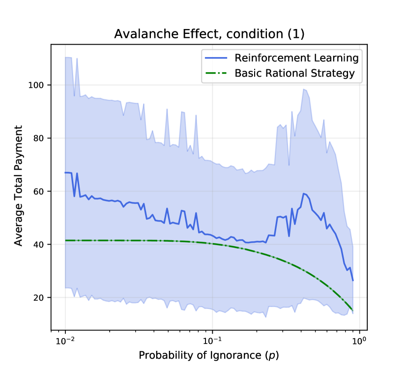
Figure 2: Expected total payment of terminal agents for varying probability of ignorance $p$ (left) and number of incoming offenders $x$ (right) averaged over ten random seeds and showing also the standard error. The figures demonstrate the Avalanche effect defined in Section 2.3.

4.3.2 Division problem

In this section, we numerically study the Division problem introduced in Section 2.4. Results for both the Time- and Group-Division problem are presented in Figure 3.

For the Time-Division problem, BRS seems to drastically overpay the learned strategy if the sorting is frequent, i.e. $T$ is large. On the other hand, when $T$ is small the willingness to pay doesn’t increase. This leads to paying only $kQ=48$ for $T=1$, while the learned strategy prefers to pay more. When the game is sorted more often, the learned strategy seems to favor lower total payments.

In the Group-Division scenario, both BRS and the learned strategy pay less in larger system. Splitting the game into several smaller thus increases the total payment of the offenders. This is in agreement with the analytic solution presented in Section 3.2.2, suggesting the incoming agents don’t impact Queue much.

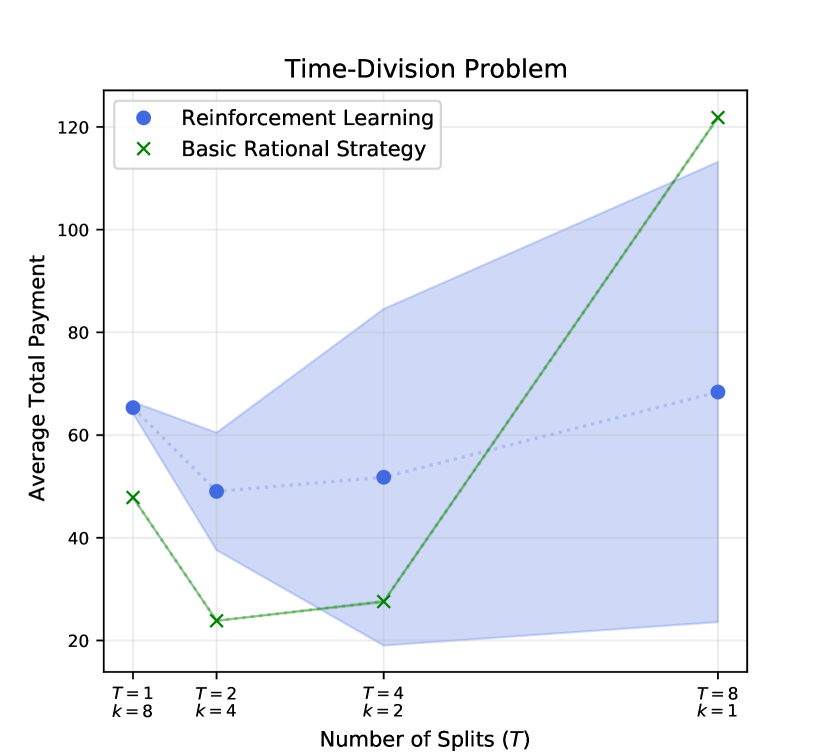
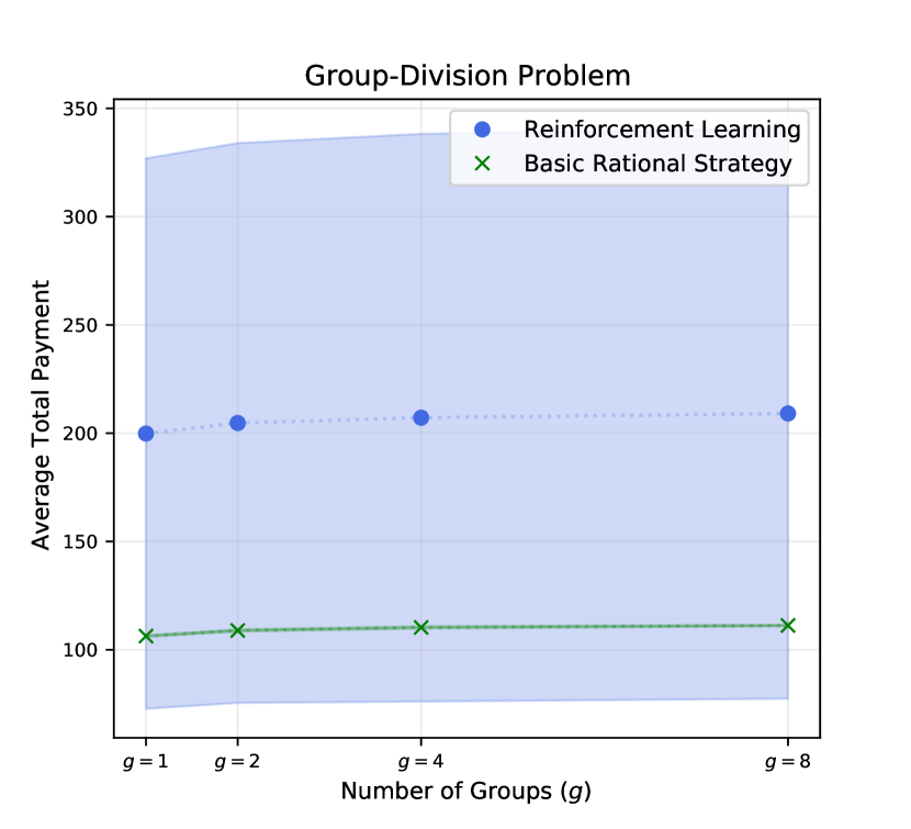
Figure 3: Expected total payment of terminal agents for varying number of sortings $T$ (left) and number of splits $g$ (right). The results are averaged over ten random seeds and the colored areas show standard error. The figures investigate the Division problem defined in Section 2.4.

4.3.3 Exploitability of Basic Rational Strategy

The BRS is a heuristic designed to capture realistic behaviour of humans. However, it is not guaranteed to make optimal decisions. In this section, we investigate exploitability of BRS. Specifically, we let 90% of the agents follow BRS, with the rest refining their strategy using PPO. We compare the expected payment of agents following each of the strategies after convergence. We present our results in Figure 4 for varying probability of ignorance $p$ and number of entering agents $x$. In all cases the learning algorithm is able to find strategy which achieves vastly lower expected payment, suggesting the BRS is quite exploitable.

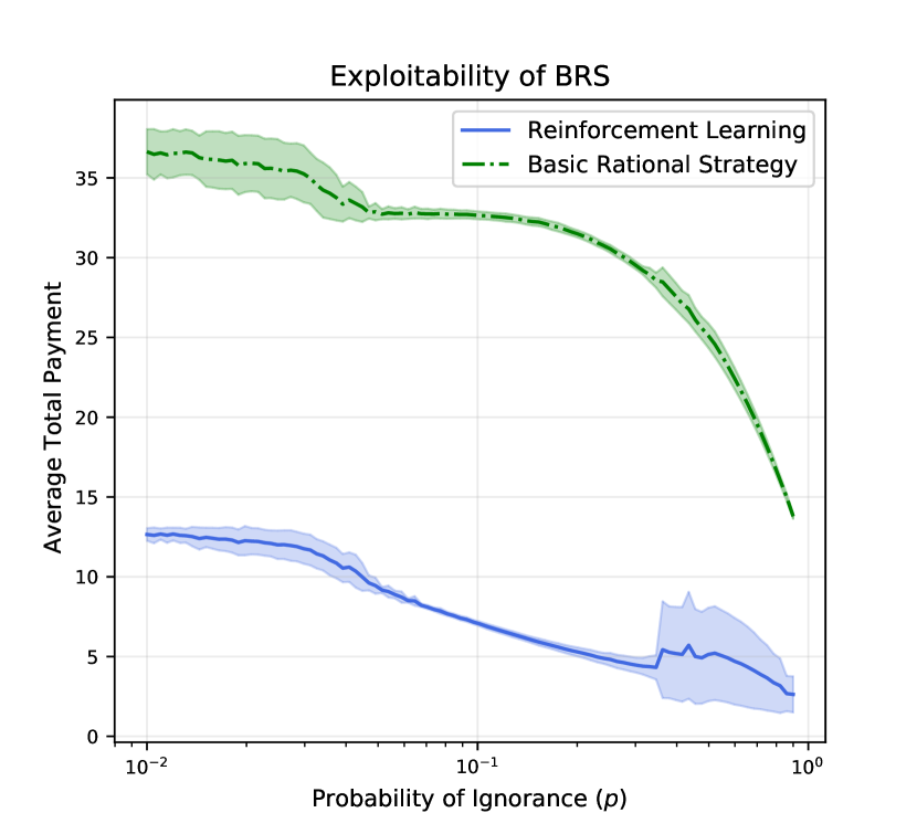
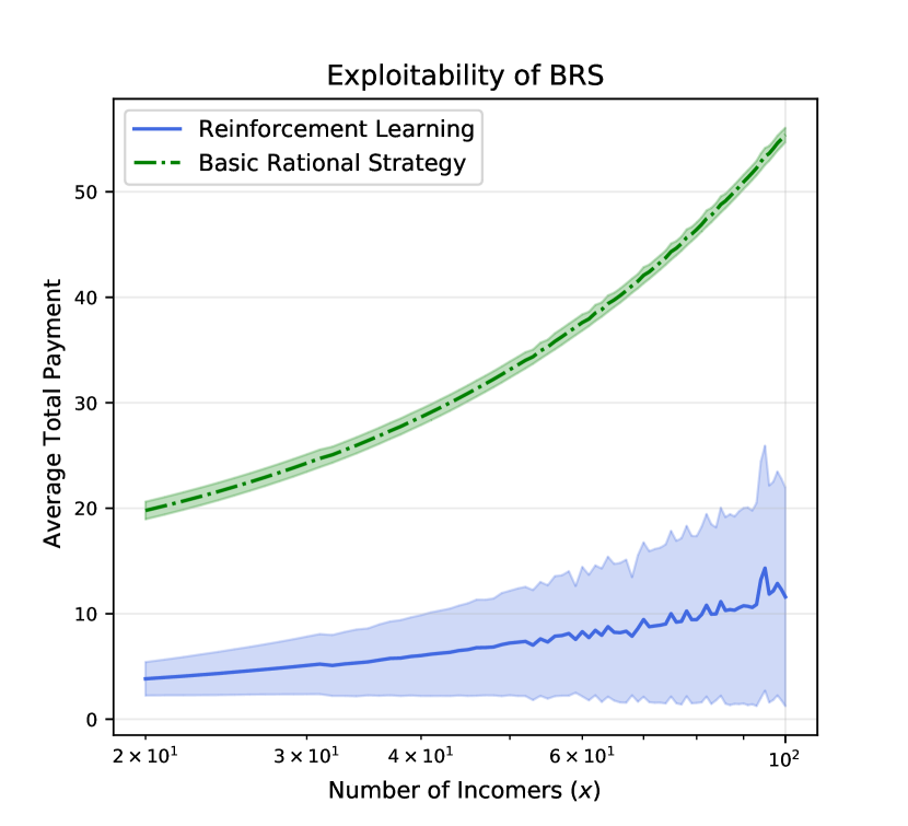
Figure 4: Expected total payment of terminal agents for varying probability of ignorance $p$ (left) and number of incoming offenders $x$ (right) averaged over ten random seeds and showing also the standard error. The training was done with 90% of agents following BRS., i.e. approximating best-response to BRS.

5 Conclusion

In this work, we suggest a simple mechanism for rule enforcing, like collecting fines for traffic violations in large cities, by a small number of administrators. We show analytically and on realistic experiments that this simple mechanism exhibits the Avalanche effect and thus supports non-cooperation of offenders. We quantify the fines collection in expectation. Finally, we present some initial results towards understanding the effective use of the administrators, i.e., the Division problem.

Future work: ⁢ Further study of the Division problem, in particular possible strengthening of Lemma 3 is our work in progress.

We see a limitation of our numerical approach in that we limit ourselves to scenarios where all agents share the same strategy $\pi_{a}$. We would like to improve on our results by having each agent follow one of a few leaders, similar to how we investigated exploitability of BRS.

Appendix 0.A Proof Of Theorem 3.1

Theorem 3.1

$\alpha(p,n,k)\geq\alpha(p,2n,2k)$ for $1\leq k<np-p$.

We will prove the theorem in a sequence of lemmas. Note that $\alpha(p,n,k)=\mathbb{P}[X\leq k]$ for $X\sim B(n-1,p)$.

Lemma 4

For random variables $X\sim B(n,p)$ and $Y\sim B(2n,p)$ and $1<k<np$, we have $\mathbb{P}[X\leq k]\geq\mathbb{P}[Y\leq 2k]$.

Proof

We make use of the Camp-Paulson approximation [9, 4] to the normal distribution for a binomial distribution which states that for $X\sim B(n,p)$

$$\left|\mathbb{P}[X\leq k]-\mathbf{\Phi}\left(\frac{c-m}{\theta}\right)\right|\leq\frac{0.007}{\sqrt{np(1-p)}},$$

where $c=(1-b)r^{\frac{1}{3}},m=1-a,\theta=\sqrt{br^{\frac{2}{3}}+a},$ $b=\frac{1}{9(k+1)},a=\frac{1}{9(n-k)},r=\frac{(k+1)(1-p)}{p(n-k)},$ and $\mathbf{\Phi}(x)=\frac{1}{\sqrt{2\pi}}{{\int}^{x}_{-\infty}}e^{-\frac{t^{2}}{2}}dt$.

Since $\mathbf{\Phi}$ is an increasing function it suffices to show the inequality between the arguments of $\mathbf{\Phi}$ for $k<np$. We define $r(n,x)=\frac{(x+1)(1-p)}{p(n-x)},c(n,x)=\left(1-\frac{1}{9(x+1)}\right)r(n,x)^{\frac{1}{3}}=\frac{9x+8}{9(x+1)}r(n,x)^{\frac{1}{3}}$, $m(n,x)=1-\frac{1}{9(n-x)}$ and $\theta(n,x)=\sqrt{\frac{1}{9(x+1)}r(n,x)^{2/3}+\frac{1}{9(n-x)}}$.

Thus we need to show that $\frac{c(n,x)-m(n,x)}{\theta(n,x)}>\frac{c(2n,2x)-m(2n,2x)}{\theta(2n,2x)}$ for $k<np$. We prove this in two parts. Our first claim will show that there is a $K_{n}<np$, where ${c(n,x)-m(n,x)}$ is zero. ∎

Claim

$c(n,x)-m(n,x)$ is an increasing function of $x$ for $0<x<n$ and there exists $K_{n}<np$ such that $c(n,x)<m(n,x)$ for all $x<K$ and $c(n,x)>m(n,x)$ for all $x>K$.

Proof

It is easy to see that for $0<x<n$, $r(x)$ and $c(x)$ are increasing functions and $m(n,x)$ is a decreasing function. Thus for $0<x<np$ we have $1>m(n,x)\geq 1-\frac{1}{9(n-np)}$ and $(1-\frac{1}{9(x+1)})\leq(1-\frac{1}{9(np+1)})$. We first find the condition for $x>0$ such that $r(n,x)<\left(\frac{y-1}{y}\right)^{3}$ for some $y>0$. Note here that we can assume that such an $x$ exists as we are assuming $p>\frac{1}{n}$. The inequality holds for all $x<\frac{np(y-1)^{3}-y^{3}(1-p)}{y^{3}(1-p)+p(y-1)^{3}}$. Since $y>0$, we have that the inequality holds for all $x<np\left(\frac{y-1}{y}\right)^{3}-1+p$. Thus for $y=9(n-np)$ we have, $c(n,x)=\frac{9x+8}{9(x+1)}\left(1-\frac{1}{9(n-np)}\right)<m(n,x)$.

$$c(n,np) = \frac{9np+8}{9(np+1)}\left(\frac{(np+1)(1-p)}{p(n-np)}\right)^{1/3}=\frac{9np+8}{9(np+1)}\left(\frac{np+1}{np}\right)^{1/3}$$

$$\geq \frac{9np+8}{9(np+1)}\left(\frac{np+1}{np}\right)^{1/3}=\frac{9np+8}{9np}\left(\frac{np}{np+1}\right)^{2/3}$$

$$= \left(1+\frac{8}{9np}\right)\left(\frac{np}{np+1}\right)^{2/3}$$

It is easy to see that $\left(1+\frac{8}{9x}\right)\left(\frac{x}{x+1}\right)^{2/3}>1$ for all $x>0$. Thus $c(n,np)>1>m(n,np)$. This proves the claim. ∎

Notice that $K_{n}$ is very close to $np$ but nevertheless lower than $np$. We are now ready to partly prove Theorem 3.1.

Lemma 5

For $0<x<\frac{K_{2n}}{2}$, $\frac{c(n,x)-m(n,x)}{\theta(n,x)}>\frac{c(2n,2x)-m(2n,2x)}{\theta(2n,2x)}$.

Proof

To do this we see some properties of $\frac{c(n,x)-m(n,x)}{\theta(n,x)}$. Individually the functions compare as follows for $1\leq x<n$.

$$\left(\frac{\theta(2n,2x)}{\theta(n,x)}\right)^{2} =\frac{1}{2}\left(\frac{x+1}{2x+1}\right)^{1/3}\frac{{(2n-2x)^{1/3}(1-p)^{2/3}+(2x+1)^{1/3}p^{2/3}}}{{(n-x)^{1/3}(1-p)^{2/3}+(x+1)^{1/3}p^{2/3}}}$$

$$\leq\frac{1}{2}\left(\frac{x+1}{2x+1}\right)^{1/3}\frac{{(2n-2x)^{1/3}(1-p)^{2/3}+(2x+2)^{1/3}p^{2/3}}}{{(n-x)^{1/3}(1-p)^{2/3}+(x+1)^{1/3}p^{2/3}}}$$

$$\leq\frac{1}{2^{2/3}}\left(\frac{x+1}{2x+1}\right)^{1/3}<1$$

Also $\frac{c(n,x)}{c(2n,2x)}=2^{1/3}\left(\frac{9x+8}{18x+8}\right)\left(\frac{2x+1}{x+1}\right)^{2/3}>1$ as this is a decreasing function for $x>0$ with its limit at $1$, and $m(n,x)-m(2n,2x)=\frac{1}{9(2n-2x)}-\frac{1}{9(n-x)}=-\frac{1}{9(2n-2x)}<0$.

Thus we have $c(2n,2x)-m(2n,2x)<c(n,x)-m(n,x)$. It follows that $K_{n}\leq\frac{K_{2n}}{2}$. Thus for $x\leq K_{n}$ we have $\frac{\theta(2n,2x)}{\theta(n,x)}\frac{c(n,x)-m(n,x)}{c(2n,2x)-m(2n,2x)}<1$ i.e.,
$\left|\frac{c(2n,2x)-m(2n,2x)}{\theta(2n,2x)}\right|\geq\left|\frac{c(n,x)-m(n,x)}{\theta(n,x)}\right|$ but both quantities are negative and so $\frac{c(2n,2x)-m(2n,2x)}{\theta(2n,2x)}\leq\frac{c(n,x)-m(n,x)}{\theta(n,x)}$. For $K_{n}<x<\frac{K_{2}n}{2}$ we have $\frac{c(2n,2x)-m(2n,2x)}{\theta(2n,2x)}\leq 0\leq\frac{c(n,x)-m(n,x)}{\theta(n,x)}$. ∎

Lemma 5 allows us to state a weaker result.

Corollary 2

For random variables $X\sim B(n,p)$ and $Y\sim B(n+\left\lceil n/p\right\rceil,p)$ and $k<\max\{\frac{n}{2},np\}$, we have $\mathbb{P}[X\leq k]\geq\mathbb{P}[Y\leq 2k]$.

Proof

The proof follows from the fact that $n+\frac{n}{p}>2n$ and $2x<(np+n)\left(\frac{9\frac{n}{p}-9np-1}{9\frac{n}{p}-9np}\right)-1+p<K_{n+\frac{n}{p}}$. ∎

Now we can complete the proof of Theorem 3.1.

Proof (of Theorem 3.1)

Notice that $c-m$ and $\theta$ are monotonically increasing in $x$. The difference between using $n$ and $2n$ is just the rate of increase. We have shown for $x<K_{2n}$, $(c-m)(n,x)\theta^{2}(2n,2x)>(c-m)(2n,2x)\theta^{2}(n,x)$. Now we show the inequality holds for $x=np$, i.e., the two functions haven’t crossed each other.

Define $r_{1}=\frac{np+1}{np},r_{2}=\frac{2np+1}{2np},b_{1}=\frac{1}{9(np+1)},b_{2}=\frac{1}{9(2np+1)}$, $a=\frac{1}{18(n-np)}$, $\theta_{1}=b_{1}r_{1}^{2/3}+2a$ and $\theta_{2}=b_{2}r_{2}^{2/3}+2a$. Thus we have

$$1\leq\frac{r_{1}}{r_{2}}=2\left(\frac{np+1}{2np+1}\right)=\frac{2b_{2}}{b_{1}}\leq 2$$ (22)

$$(c-m)(n,np)\theta^{2}(2n,2np)-(c-m)(2n,2np)\theta^{2}(n,np)$$

$$=((1-b_{1})r_{1}^{1/3}-1+2a)\theta_{2}-((1-b_{2})r_{2}^{1/3}-1+a)\theta_{1}$$

$$=\frac{2^{1/3}(2np+1)^{1/3}(9np+8)(n-np)-2^{2/3}(np+1)^{1/3}(18np+8)(n-np)}{81[(np+1)(2np+1)]^{2/3}2np(n-np)}$$

$$\quad+\frac{2[2np(np+1)]^{2/3}-2[np(2np+1)]^{2/3}+18(np+1)2^{1/3}[np(2np+1)]^{2/3}]^{2/3}}{81[(2np+1)(np+1)]^{2/3}(2np)(n-np)2}$$

$$\quad-\frac{18(2np+1)[2np(np+1)]^{2/3}}{81[(2np+1)(np+1)]^{2/3}(2np)(n-np)2}$$

$$\quad+\frac{18(n-np)[np(np+1)]^{1/3}(2np+1)^{2/3}-9(n-np)[2np(2np+1)]^{1/3}(np+1)^{2/3}}{81(n-np)[(np+1)(2np+1)]^{2/3}(2np)}$$

$$\quad+\frac{9[(np+1)(2np+1)]^{2/3}(2np)+2(np+1)^{2/3}(2np+1)^{1/3}(2np)^{1/3}}{81(n-np)[(np+1)(2np+1)]^{2/3}(2np)2}$$

$$\quad-\frac{2(np+1)^{1/3}(2np+1)^{2/3}(np)^{1/3}}{81(n-np)[(np+1)(2np+1)]^{2/3}(2np)2}$$

Using $p^{3}-q^{3}=(p-q)(p^{2}+pq+q^{2})$ we have,

$$2^{1/3}(2x+1)^{1/3}(9x+8)-9[2x(2x+1)]^{1/3}(x+1)^{2/3}$$

$$=2^{1/3}(2x+1)^{1/3}[8+9x^{1/3}(x^{2/3}-(x+1)^{2/3}]$$

$$=2^{1/3}(2x+1)^{1/3}\left[8+\left(\frac{-9x^{1/3}(2x+1)}{x^{4/3}+x^{2/3}(x+1)^{2/3}+(x+1)^{4/3}}\right)\right]$$ (23)

and,

$$18[x(x+1)]^{1/3}(2x+1)^{2/3}-2^{2/3}(x+1)^{1/3}(18x+8)$$

$$=(x+1)^{1/3}[8+18x^{1/3}((2x+1)^{2/3}-(2x)^{2/3}]$$

$$=(x+1)^{1/3}\left[8+\left(\frac{18x^{1/3}(4x+1)}{(2x+1)^{4/3}+(2x(2x+1))^{2/3}+(2x)^{4/3}}\right)\right]$$ (24)

Note that the sum of 0.A and 24 is positive for $x\geq 1$. Thus all the terms with $n-np$ in the numerator add up to a positive quantity. The only other negative component is $\frac{18(np+1)2^{1/3}[np(2np+1)]^{2/3}-18(2np+1)[2np(np+1)]^{2/3}}{81[(2np+1)(np+1)]^{2/3}(2np)(n-np)2}$, which is dominated by $\frac{9[(np+1)(2np+1)]^{2/3}(2np)}{81(n-np)[(np+1)(2np+1)]^{2/3}(2np)2}$.

Thus $\frac{c(n,np)-m(n,np)}{\theta(n,np)}\Bigg{/}\frac{c(2n,2np)-m(2n,2np)}{\theta(2n,2np)}\geq\frac{\theta(n,np)}{\theta(2n,2np)}\geq 1.$

∎

Parameter	Value	Description
$\varepsilon$	0.05	Policy update clipping
$\gamma$	1	Reward discounting
$\lambda$	0.95	Advantage decay factor
$N_{\rm train}$	32	Number of training updates per cycle
$N_{\rm epochs}$	512	Number of training epochs
$N_{\rm train}$	$2\cdot 10^{4}$	Train buffer size
$\alpha_{\rm actor}$	$3\cdot 10^{-4}$	Actor learning rate
$\alpha_{\rm critic}$	$10^{-3}$	Critic learning rate
$c_{\rm H}$	$10^{-3}$	Entropy regularization weight
$\overline{c}$	0.1	Gradient norm clipping

Table 1: Hyperparameters of the learning algorithm.

Appendix 0.B Learning Algorithm

The shared strategy $\pi_{a}$ is represented by a neural network and trained from trajectories of all terminal agents. When selecting the strategy for a Round, we mask all actions which would lead to $m_{a}+\mu_{a}>F$. This makes the agents unable to overpay the fine $F$. We use fully-connected networks for both the actor and the critic. Both take as input the observation of $a$ in Round, i.e. $(n_{a},t_{a},m_{a})$. The actor network has two hidden layers with four hidden units, and the critic has three hidden layers with 32 units each, all using the ReLU activation function. The rest of the hyperparameters are given in Table 1.

References

- [1] Loebl M. Sychrovsky D., Desai S. Promoting non-cooperation through ordering. In The 14th Workshop on Optimization and Learning in Multiagent Systems, OptLearnMAS, 2023.
- [2] A. Lee Chiam C., Li J. The Bidding Elimination Game. 2020.
- [3] de Campagnolle M. R. Kobylanski M., Quenez† M. Dynkin games in a general framework, 2013.
- [4] Spencer Greenberg and Mehryar Mohri. Tight lower bound on the probability of a binomial exceeding its expectation. Statistics & Probability Letters, 86:91–98, 2014.
- [5] John Schulman, Filip Wolski, Prafulla Dhariwal, Alec Radford, and Oleg Klimov. Proximal policy optimization algorithms. CoRR, abs/1707.06347, 2017.
- [6] Dibya Ghosh, Marlos C. Machado, and Nicolas Le Roux. An operator view of policy gradient methods. In Proceedings of the 34th International Conference on Neural Information Processing Systems, NIPS’20, Red Hook, NY, USA, 2020. Curran Associates Inc.
- [7] Bowen Baker, Ingmar Kanitscheider, Todor Markov, Yi Wu, Glenn Powell, Bob McGrew, and Igor Mordatch. Emergent tool use from multi-agent autocurricula. In International Conference on Learning Representations, 2020.
- [8] Marc Lanctot, Vinicius Zambaldi, Audrunas Gruslys, Angeliki Lazaridou, Karl Tuyls, Julien Perolat, David Silver, and Thore Graepel. A unified game-theoretic approach to multiagent reinforcement learning. In I. Guyon, U. Von Luxburg, S. Bengio, H. Wallach, R. Fergus, S. Vishwanathan, and R. Garnett, editors, Advances in Neural Information Processing Systems, volume 30. Curran Associates, Inc., 2017.
- [9] Scott M. Lesch and Daniel R. Jeske. Some suggestions for teaching about normal approximations to poisson and binomial distribution functions. The American Statistician, 63(3):274–277, 2009.