Nambu-Goto Strings with a null symmetry and contact structure

Abstract

We study the classical dynamics of the Nambu-Goto strings with a null symmetry in curved spacetimes admitting a null Killing vector field. The Nambu-Goto equation is reduced to first-order ordinary differential equations and is always integrable in contrast to the case of non-null symmetries where integrability requires additional spacetime symmetries. It is found that in the case of null symmetry, an almost contact structure associated with the metric dual $1$-form $\eta$ of the null Killing vector field emerges naturally. This structure determines the allowed class of string worldsheets in such a way that the tangent vector fields of the worldsheet lie in $\ker{\differential{\eta}}$. In the special case that the almost contact structure becomes a contact structure, its Reeb vector field completely characterizes the worldsheet. We apply our formulation to the strings in the pp -waves, the Einstein static universe and the Gödel universe. We also study their worldsheet geometry in detail.

I Introduction

Strings, one-dimensional objects, appear in various areas of physics. In cosmology, one-dimensional topological defects called the cosmic strings are supposed to have formed in the early universe (e.g. [1]). In string theories, microscopic strings are considered to be the fundamental elements (e.g. [2]).

The string dynamics is characterized by a two-dimensional worldsheet in spacetime and is in most cases governed by the Nambu-Goto action. The equation of motion is given by a set of partial differential equations, and is therefore generally difficult to solve. However, a simplification occurs when the string worldsheet has a symmetry called cohomogeneity one (C1) [3]. The C1 symmetry means that the string worldsheet shares a Killing vector field with the spacetime, or more precisely, a Killing vector field of the spacetime is tangent to the worldsheet.

String dynamics with C1 symmetry have been widely studied in various contexts. One example is the stationary strings. They move in stationary spacetimes and sweep the worldsheets tangent to the timelike Killing vector fields. The stationary (rotating) strings in black hole spacetimes have been studied extensively with astrophysical and geometrical interests [4, 5, 6, 7, 8]. Another example can be found in the context of the AdS/CFT correspondence. The C1 string ansatz is effectively used in curved backgrounds, and then the string motion is found to be chaotic [9, 10, 11, 12, 13, 14, 15]. The classification problem of C1 strings are also studied in some highly symmetric spacetimes such as Minkowski spacetime [3], five-dimensional anti-de Sitter spacetime $\text{AdS}^{5}$ [16] and higher-dimensional flat spacetimes $\mathbb{R}^{n,1}$ [17]. The concept of the cohomogeneity one (C1) symmetry has been extended to higher dimensional objects such as membranes [18, 19].

In previous studies of C1 strings, the Killing vector field tangent to the worldsheet is assumed to be timelike or spacelike. In this case, the Nambu-Goto equation of motion is reduced to the geodesic equation with respect to a certain metric weighted by the squared norm of the Killing vector field [3, 20]. If the metric admits a sufficient number of Killing vector fields and Killing tensor fields, the geodesic equation admits a sufficient number of conserved quantities and is then integrable in quadrature. Indeed, it has been clarified that the C1 string dynamics is integrable in some highly symmetric spacetimes [21, 20, 17]. On the other hand, C1 strings with null tangent Killing vector fields have not been well studied. Strings with a null symmetry may be interesting, for example, in pp -waves, which attract much attention in string theories [22, 23, 24, 25].

The purpose of this paper is to formulate the dynamics of Nambu-Goto strings with a null C1 symmetry in curved spacetimes and to study the dynamics, in particular, the integrability and the extrinsic geometry of the worldsheets.

We will see that the Nambu-Goto equation reduces to ordinary differential equations (ODEs). While the ODEs in the case of non-null C1 symmetry are second order, the null C1 ODEs are first order. The Nambu-Goto equation is always integrable in the null case, in contrast to the non-null case where integrability requires additional symmetries.

We will also find that an almost contact structure associated with the metric dual $1$-form of the null Killing vector field emerges naturally. In the special case that the almost contact structure becomes the contact structure, its Reeb vector field completely characterizes the worldsheet.

Contact structures appear in various areas of physics: for example, classical dynamics [26], thermodynamics [27, 28] and electromagnetism [29]. Contact and almost contact structures are lower level structures of the Sasaki structure [30, 31], which is attracting renewed attention in the context of the AdS/CFT correspondence [32]. Three-dimensional Sasaki or quasi-Sasaki manifolds are effectively used to construct Gödel-type solutions in Einstein-Maxwell-scalar field theories [33] and a generalized Einstein’s static universe [34]. Then, our results suggest that the lower level structures such as (almost) contact structure may also be useful in general relativity as well.

The paper is organized as follows. In the following section, we reduce the Nambu-Goto equation and gauge conditions to first-order ordinary differential equations. In Sec. III, we solve the equations in general, and then discuss the relation with the (almost) contact structure. In Sec. IV, we study the extrinsic geometry of the worldsheet, in particular, the second fundamental form. In Sec. V, we apply our formulation to the strings in the pp -waves, the Einstein static universe and the Gödel universe and investigate their worldsheet geometry. Sec. VI is devoted to conclusions.

II Equation of motion

II.1 Equation of motion in double null coordinates

Let $(\mathcal{M},g)$ be a $(D+1)$-dimensional spacetime furnished with a Lorentzian metric $g$. A string sweeps the so-called worldsheet $\mathcal{S}$, which is a two-dimensional timelike surface

$$x^{\mu}=x^{\mu}(\zeta^{1},\zeta^{2})\quad(\mu=0,\dots,D)$$ (1)

where $x^{\mu}$ are spacetime coordinates or embedding functions of the worldsheet and $\zeta^{a}~{}(a=1,2)$ are worldsheet coordinates. We assume that the string dynamics is governed by the Nambu-Goto action

$$S=\int\sqrt{-\gamma}\,\differential{\zeta^{1}}\differential{\zeta^{2}},\quad\gamma\coloneqq\det\gamma_{ab},$$ (2)

where $\gamma_{ab}$ is the worldsheet metric given by

$$\gamma_{ab}=g_{\mu\nu}\partialderivative{x^{\mu}}{\zeta^{a}}\partialderivative{x^{\nu}}{\zeta^{b}}.$$ (3)

Varying the action, we obtain the equations of motion

$$\partialderivative{\zeta^{a}}\quantity(\sqrt{-\gamma}\,\gamma^{ab}\partialderivative{x^{\mu}}{\zeta^{b}})+\sqrt{-\gamma}\,\gamma^{ab}\Gamma^{\mu}{}_{\nu\lambda}\partialderivative{x^{\nu}}{\zeta^{a}}\partialderivative{x^{\lambda}}{\zeta^{b}}=0,$$ (4)

where $\Gamma^{\mu}{}_{\nu\lambda}$ is the Christoffel symbol.

In this paper, we take both of the worldsheet coordinates $\zeta^{1},\zeta^{2}$ to be null. Then the worldsheet metric has a cross term only:

$$\differential{s}^{2}=\gamma_{ab}\differential{\zeta^{a}}\differential{\zeta^{b}}=2\,\gamma_{12}(\zeta^{1},\zeta^{2})\differential{\zeta^{1}}\differential{\zeta^{2}},\quad\gamma_{12}(\zeta^{1},\zeta^{2})\neq 0,$$ (5)

and the equation of motion (4) takes the form

$$\partialderivative{x^{\nu}}{\zeta^{2}}\nabla_{\nu}\partialderivative{x^{\mu}}{\zeta^{1}}=0,$$ (6)

where $\nabla$ is the Levi-Civita connection on $(\mathcal{M},g)$. We note that the metric function $\gamma_{12}(\zeta^{1},\zeta^{2})$ does not appear in the equation of motion.

II.2 Cohomogeneity-one strings with a null Killing vector field

We define cohomogeneity-one strings with a null Killing vector field and derive the equations of motion and the constraint equations. It is convenient to use the language of differential forms, where for a $1$-form $A$, the exterior derivative of $A$ is expressed with the Levi-Civita connection $\nabla$ as

$$\quantity(\differential A)_{\mu\nu}=\quantity(A_{\nu,\mu}-A_{\mu,\nu})=2\nabla_{[\mu}A_{\nu]},$$ (7)

and, for a $p$-form $B$, the interior product with a vector field $X$ is given by

$$\iota_{X}B\coloneqq B(X,\underbrace{\,\cdot\,,\dots,\,\cdot\,}_{\text{$p-1$ slots}}).$$ (8)

We assume that the spacetime $(\mathcal{M},g)$ admits a null Killing vector field $k$, which satisfies

$$\nabla_{(\mu}k_{\nu)}=0,\qquad g_{\mu\nu}k^{\mu}k^{\nu}=0.$$ (9)

Let $\eta$ be the metric dual $1$-form of $k$:

$$\eta\coloneqq g(k,\,\cdot\,)=k_{\mu}\differential{x}^{\mu}.$$ (10)

The covariant derivative of $k$ is given by

$$\nabla_{\mu}k_{\nu}=\frac{1}{2}\quantity(\differential{\eta})_{\mu\nu},$$ (11)

where Eqs. (7) and (9) are used. It follows from Eq. (9) that the null Killing vector field $k$ satisfies geodesic equation

$$k^{\nu}\nabla_{\nu}k^{\mu}=0.$$ (12)

Using Eq. (11), we can express this equation as

$$\iota_{k}\differential{\eta}=0.$$ (13)

A cohomogeneity-one (C1) string is defined as a string whose worldsheet is tangent to a Killing vector field. In this paper, the tangent Killing vector field is assumed to be null, namely $k$. For this tangent null Killing vector field, we take the null coordinate $\zeta^{1}$ on the worldsheet $\mathcal{S}$ so that

$$\partialderivative{x^{\mu}}{\zeta^{1}}=k^{\mu},$$ (14)

then the equation of motion (6) is written as

$$\iota_{l}\differential{\eta}=0,$$ (15)

where $l$ denote the other null tangent vector field $\partialderivative*{\zeta^{2}}$:

$$l^{\mu}\coloneqq\partialderivative{x^{\mu}}{\zeta^{2}}.$$ (16)

In the spacetimes with $\differential{\eta}=0$, which are known as the pp -waves (see Sec. V), the equation of motion (15) is trivial.

We now consider the case $\differential{\eta}\neq 0$. Let $r$ be $\rank\differential{\eta}$, which is given as the maximum integer $r$ such that

$$\quantity(\differential{\eta})^{r}\coloneqq\underbrace{\differential{\eta}\wedge\dots\wedge\differential{\eta}}_{\text{$r$ factors}}\neq 0,\qquad 2r\leqq\dim\mathcal{M}=D+1.$$ (17)

Then it follows that

$$\eta\wedge\quantity(\differential{\eta})^{r}\neq 0,$$ (18)

because the equation of motion (15) implies that

$$\iota_{l}\quantity[\eta\wedge\quantity(\differential{\eta})^{r}]=\iota_{l}\eta\,\quantity(\differential{\eta})^{r}-\eta\wedge\quantity[\iota_{l}\quantity(\differential{\eta})^{r}]=\iota_{l}\eta\,\,\quantity(\differential{\eta})^{r}\neq 0,$$ (19)

where we have used $\iota_{l}\eta=g_{\mu\nu}k^{\mu}l^{\nu}=\gamma_{12}\neq 0$. Eq. (18) and Darboux’s theorem ensure the existence of local coordinates

$$y^{1},\dots,y^{r},z^{1},\dots,z^{r},w,w^{1},\dots,w^{s-1}$$ (20)

such that

$$\eta=y^{1}\differential{z^{1}}+\dots+y^{r}\differential{z^{r}}+\differential{w},$$ (21)

where $s$ is $\operatorname{corank}_{\mathcal{M}}\differential{\eta}$ defined by

$$\operatorname{corank}_{\mathcal{M}}\differential{\eta}\coloneqq\dim\mathcal{M}-2\rank\differential{\eta}$$ (22)

In the coordinates (20), the null Killing vector field $k$ is expressed as

$$k=\sum_{i=1}^{s-1}k^{w^{i}}\partialderivative{w^{i}},$$ (23)

because it satisfies Eq. (13) and the null condition $g(k,k)=\iota_{k}\eta=0$. Therefore, $s-1$ must be greater than or equal to $1$, and hence

$$s=\operatorname{corank}_{\mathcal{M}}\differential{\eta}\geq 2.$$ (24)

We consider the string worldsheet in the coordinates (20). It follows from Eqs. (14) to (16) and Eq. (23) that

$$\partialderivative{y^{i}}{\zeta^{a}}=\partialderivative{z^{i}}{\zeta^{a}}=0\quad(i=1,\dots,r).$$ (25)

This implies that the worldsheet $\mathcal{S}$ is confined on a submanifold $\mathcal{W}$ specified by

$$y^{i}=\text{const.},\quad z^{i}=\text{const.}\quad(i=1,\dots,r).$$ (26)

The submanifold $\mathcal{W}$ is characterized by the kernels of $\differential{\eta}_{p}~{}(p\in\mathcal{M})$, which is defined as

$$\ker\differential{\eta}_{p}\coloneqq\quantity{X\in T_{p}(\mathcal{M})\,|\,\iota_{X}\differential{\eta}_{p}=0}.$$ (27)

Indeed, it follows from Eq. (21) and (26) that, for any point $p\in\mathcal{W}$,

$$T_{p}(\mathcal{W})=\ker\differential{\eta}_{p},$$ (28)

and then, we find that the submanifold $\mathcal{W}$ is an integral manifold of the distribution $p\mapsto\ker\differential{\eta}_{p}$ for $p\in\mathcal{M}$. In the special case that $\operatorname{corank}_{\mathcal{M}}\differential{\eta}=2$, which implies that $\dim\mathcal{W}=2$, the worldsheet $\mathcal{S}$ is the submanifold $\mathcal{W}$ itself so that the worldsheet $\mathcal{S}$ is an integral manifold of the distribution.

We turn to the coordinate condition (14) to fix the residual gauge freedom of the worldsheet coordinate $\zeta^{2}$. Since Eq. (14) shows that $\partialderivative*{\zeta^{1}}$ is a Killing vector field on the worldsheet, the induced metric does not depend on $\zeta^{1}$, and consequently, we find that the worldsheet metric is flat; indeed,

$$\differential{s}^{2}=\gamma_{ab}\differential{\zeta^{a}}\differential{\zeta^{b}}=2\,\gamma_{12}(\zeta^{2})\,\differential{\zeta^{1}}\differential{\zeta^{2}}=2\differential{\zeta^{1}}\differential{\tilde{\zeta}^{2}},\quad\differential{\tilde{\zeta}^{2}}\coloneqq\gamma_{12}(\zeta^{2})\differential{\zeta^{2}}.$$ (29)

This implies that we can take the worldsheet coordinate $\zeta^{2}$ so that

$$\gamma_{12}=\iota_{l}\eta=1.$$ (30)

We impose this condition on the coordinate $\zeta^{2}$. It should be noted that the coordinate $\zeta^{2}$ is past directed when the coordinate $\zeta^{1}$, or the null Killing vector field $k$, is future directed. This condition is convenient for discussing the (almost) contact structures (see Subsec. III.3).

Eqs. (14) and (30) and the nullness of the null tangent vector field $l$,

$$g_{\mu\nu}l^{\mu}l^{\nu}=0,$$ (31)

specify the worldsheet coordinates $(\zeta^{1},\zeta^{2})$ up to the addition of constants. These are the gauge conditions to be solved with the equation of motion (15).

In the remainder of this paper, the worldsheet coordinates $(\zeta^{1},\zeta^{2})$ are denoted by $(\lambda,\sigma)$.

II.3 Reduction to ordinary differential equations

We construct a coordinate system in the $(D+1)$-dimensional spacetime $(\mathcal{M},g)$ separate from those used in the previous subsection, so that the equation of motion (15) and the gauge conditions (14), (30) and (31) are reduced to ordinary differential equations. The coordinate system is set up by utilizing the null Killing vector field $k$. The associated one-parameter group of isometries is denoted by $\varphi_{v}$.

First, we take a hypersurface $\Sigma_{0}$ transversal to the orbits of $\varphi_{v}$, that is, each orbit intersects with $\Sigma_{0}$ once. Then we can uniquely specify the orbits using the intersections with $\Sigma_{0}$. Let $\mathcal{O}_{p}$ be the orbit with the intersection $p\in\Sigma_{0}$. The set of orbits $\quantity{\mathcal{O}_{p}}_{p\in\Sigma_{0}}$ fill the whole spacetime without any redundancy.

Next, we consider the hypersurfaces $\Sigma_{v}~{}(v\in\mathbb{R})$ that are given by the action of $\varphi_{v}$ on $\Sigma_{0}$. Then it follows that the set of the hypersurfaces $\quantity{\Sigma_{v}}_{v\in\mathbb{R}}$ foliates the whole spacetime.

Finally, we specify each point in $\mathcal{M}$ by the hypersurface $\Sigma_{v}$ and orbit $\mathcal{O}_{p}$ on which the point lies. Let $(x^{1},\dots,x^{D})$ be the coordinates of the intersection $p$ on $\Sigma_{0}$. Then the point in $\mathcal{M}$ is labeled by $(v,x^{1},\dots,x^{D})$ as shown in Fig. 1. This is the coordinate system employed in this paper. We should note that there is a freedom in choosing the hypersurface $\Sigma_{0}$ and the coordinate system $(x^{1},\dots,x^{D})$ on it.

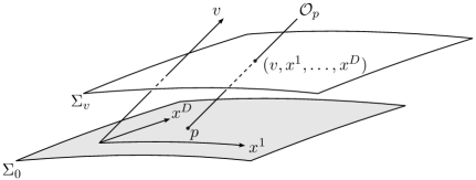
Figure 1: The coordinates $(v,x^{1},\dots,x^{D})$ of a point in the spacetime $\mathcal{M}$. The coordinate $v$ specifies the hypersurface $\Sigma_{v}$ and $x^{1},\dots,x^{D}$ specify the intersection $p$ of the orbit $\mathcal{O}_{p}$ with $\Sigma_{0}$.

In the coordinate system $(v,x^{1},\dots,x^{D})$, the vector field $\partialderivative*{v}$ coincides with the null Killing vector field $k$ by definition. Then Eq. (14) is solved as

$$v(\lambda,\sigma)=\lambda+v_{0}(\sigma),\quad x^{i}(\lambda,\sigma)=x^{i}(\sigma)\quad(i=1,\dots,D),$$ (32)

and the metric is written as

$$\differential{s}^{2}=2\eta_{i}(x)\differential{x}^{i}\differential{v}+h_{ij}(x)\differential{x}^{i}\differential{x}^{j},$$ (33)

where $\eta_{i}(x)$ and $h_{ij}(x)$ are functions of $x^{1},\dots,x^{D}$. From these equations, the other null tangent vector field $l\coloneqq\partialderivative*{\sigma}$ is given by

$$l=v_{0}^{\prime}(\sigma)\partialderivative{v}+x^{i}{}^{\prime}(\sigma)\partialderivative{x^{i}}\eqqcolon v_{0}^{\prime}(\sigma)k+\hat{l},$$ (34)

and the metric dual $1$-form $\eta$ of $k$ is given by

$$\eta=\eta_{i}(x)\differential{x^{i}}.$$ (35)

Thus the equation of motion (15), the gauge conditions (30) and (31) reduce to the following ordinary differential equations for $v_{0}(\sigma)$ and $x^{i}(\sigma)$,

$$\iota_{\hat{l}}\differential{\eta}=0,$$ (36)

$$\iota_{\hat{l}}\,\eta=1,$$ (37)

$$2v^{\prime}_{0}\,\iota_{\hat{l}}\,\eta+h(\hat{l},\hat{l})=0.$$ (38)

We regard Eqs. (36) and (37) as the equations that determine a curve $\mathcal{C}:\sigma\mapsto(x^{1}(\sigma),\dots,x^{D}(\sigma))$ on $\Sigma_{0}$ whose tangent vector is given by $\hat{l}$ in Eq. (34). This curve is clearly the intersection of the worldsheet (32) with the hypersurface $\Sigma_{0}$ given by $v=0$ (see Fig. 2). If we have a solution $x^{i}(\sigma)$ of Eqs. (36) and (37), Eq. (38) can be easily solved by quadrature

$$v_{0}(\sigma)=-\frac{1}{2}\int h(\hat{l},\hat{l})\differential{\sigma}.$$ (39)

Thus our main interest is to solve Eqs. (36) and (37), and obtain the curve $\mathcal{C}$, the intersection of the string worldsheet $\mathcal{S}$ and the hypersurface $\Sigma_{0}$.

Figure 2: The curve $\mathcal{C}$ given by the intersection of the worldsheet $\mathcal{S}$ with the hypersurface $\Sigma_{0}$. The diagonal lines are the orbits generated by the null Killing vector field $k$. The vector $l$ is the other null tangent vector. The projection $\hat{l}$, along $k$, of $l$ onto the $\Sigma_{0}$ gives the tangent vector of the curve.

III General solutions and almost contact structure

We solve Eqs. (36) and (37) on the hypersurface $\Sigma_{0}$ to obtain the curve $\mathcal{C}$ given by the intersection of the string worldsheet with $\Sigma_{0}$. The $1$-form $\eta$ appearing in these equations is expressed only with the hypersurface coordinates $x^{1},\dots,x^{D}$ as in Eq. (35). Then the $1$-form $\eta$ can be regarded as the one on the hypersurface $\Sigma_{0}$. This allows us to take certain coordinates on $\Sigma_{0}$ such that Eqs. (36) and (37) are easily solved. In the case that the hypersurface $\Sigma_{0}$ is odd-dimensional, the $1$-form $\eta$ provides the hypersurface $\Sigma_{0}$ with an almost contact structure, which is reviewed in Appendix A. With respect to the almost contact structure, we examine the geometric structure of the general solutions.

III.1 The case $\mathrm{d}\eta=0$

In the case $\differential{\eta}=0$, the Poincaré lemma ensures the existence of a function $\varPhi(x^{1},\dots,x^{D})$ on the hypersurface $\Sigma_{0}$ such that $\eta=\differential{\varPhi}$. Then, taking new local coordinates $w,w^{1},\dots,w^{D-1}$ on $\Sigma_{0}$ such that

$$w=\varPhi(x^{1},\dots,x^{D}),$$ (40)

we can readily solve Eqs. (36) and (37), so that the curve $\mathcal{C}:(w(\sigma),w^{1}(\sigma),\dots,w^{D-1}(\sigma))$ is given by

$$w(\sigma)=\sigma+w_{0},\quad w^{1}(\sigma),\dots,w^{D-1}(\sigma):\text{arbitrary},$$ (41)

where $w_{0}$ is a constant.

III.2 The case $\mathrm{d}\eta\neq 0$

Using the same arguments as in Subsec. II.2, we can take local coordinates

$$y^{1},\dots,y^{r},z^{1},\dots,z^{r},w,w^{1},\dots,w^{s-1}$$ (42)

on the hypersurface $\Sigma_{0}$ such that

$$\eta=y^{i}\differential{z^{i}}+\differential{w},$$ (43)

where $r$ is the rank of $\differential{\eta}$ and $s$ is the corank of $\differential{\eta}$ associated with $\Sigma_{0}$,

$$s=\operatorname{corank}_{\Sigma_{0}}\differential{\eta}=\dim\Sigma_{0}-2\rank\differential{\eta}=D-2r.$$ (44)

It follows from Eq. (36) that $(2r+1)$-form $\eta\wedge\quantity(\differential{\eta})^{r}$ does not vanish on the $D$-dimensional hypersurface $\Sigma_{0}$. This implies that $D\geqq 2r+1$, and therefore,

$$\operatorname{corank}_{\Sigma_{0}}\differential{\eta}\geqq 1.$$ (45)

In the Darboux coordinates (42), we can readily solve Eqs. (36) and (37) so that the curve $\mathcal{C}:(y^{i}(\sigma),z^{i}(\sigma),w(\sigma),w^{j}(\sigma))$ is given by

$$y^{i}(\sigma),z^{i}(\sigma):\text{constant},\quad w(\sigma)=\sigma+w_{0},\quad w^{j}(\sigma):\text{arbitrary}.$$ (46)

In the case that $\operatorname{corank}_{\Sigma_{0}}\differential{\eta}=1$, the solution does not involve any arbitrary functions. This solution corresponds to that of the case $\operatorname{corank}_{\mathcal{M}}\differential{\eta}=2$ in Subsec. II.2, where the worldsheet is given as an integral manifold of the distribution $p\mapsto\ker\differential{\eta}_{p}~{}(p\in\mathcal{M})$.

III.3 Geometric structure of the general solutions

In this subsection we assume that the hypersurface $\Sigma_{0}$ is odd-dimensional. Then the $1$-form $\eta$ provides $\Sigma_{0}$ with an almost contact structure $(\varphi,\xi,\eta)$: a triplet of $(1,1)$-tensor $\varphi$, a vector field $\xi$ and the $1$-form $\eta$ such that

$$\iota_{\xi}\eta =1,$$ (47)

$$\varphi^{2} =-1+\xi\otimes\eta.$$ (48)

Indeed, the vector field $\xi$ is given so that Eq. (47) holds for the $1$-form $\eta$, and the $(1,1)$-tensor $\varphi$ is constructed from $\eta$ and $\xi$ (see Appendix A). We should note that the vector field $\xi$ is not unique; there is a freedom to add vector field $\tilde{\xi}$ which satisfies $\iota_{\tilde{\xi}}\,\eta=0$.

We examine the general solutions obtained in the previous subsections in terms of the almost contact structure $(\varphi,\xi,\eta)$. To this aim, we choose the vector field $\xi$ so that it satisfies

$$\iota_{\xi}\differential{\eta}=0.$$ (49)

in addition to Eq. (47). Then it is obvious that the curve $\mathcal{C}$, the intersection of the worldsheet $\mathcal{S}$ with the hypersurface $\Sigma_{0}$, is given as an integral curve of the vector field $\xi$ (see Fig. 3). Thus to solve the C1 string equations of motion is to find an almost contact structure $(\varphi,\xi,\eta)$ such that the vector field $\xi$ satisfies Eq. (49). We note that the vector field $\xi$ is not unique in general even though Eq. (49) is imposed.

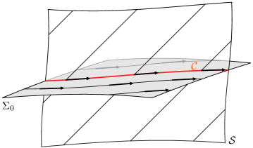
Figure 3: The geometric structure of the general solutions. In the case that $\dim\Sigma_{0}$ is odd, the curve $\mathcal{C}$, the intersection of the worldsheet $\mathcal{S}$ with the hypersurface $\Sigma_{0}$, is given as an integral curve of the vector field $\xi$ of an almost contact structure $(\varphi,\xi,\eta)$ that satisfies Eqs. (47) and (49).

The case $\operatorname{corank}_{\Sigma_{0}}\differential{\eta}=1$ is special in the sense that the almost contact structure $(\varphi,\xi,\eta)$ becomes a contact structure. A $(2r+1)$-dimensional manifold with a $1$-form $\eta$ of $\rank\differential{\eta}=r$ that satisfies $\eta\wedge\quantity(\differential{\eta})^{r}\neq 0$ is said to have a contact structure with a contact form $\eta$ (see Appendix A). In this case, the vector field $\xi$ satisfying Eqs. (47) and (49) is uniquely determined and is called the Reeb vector field. In the Darboux coordinates (42), the Reeb vector field $\xi$ is given by

$$\xi=\partialderivative{w}.$$ (50)

The unique determination of the vector field $\xi$ corresponds to the fact that the string solution does not include any arbitrary functions discussed in the previous subsection.

IV Extrinsic geometry of the worldsheet

We investigate the second fundamental form of the string worldsheet $\mathcal{S}$, which requires careful treatment because the codimension of $\mathcal{S}$, denoted by $\operatorname{codim}\mathcal{S}$, may be equal to or larger than two. The foundations are given in Appendix B.

Let $N_{I}~{}(I=1,\dots,\operatorname{codim}\mathcal{S})$ be independent normal vector fields of the worldsheet $\mathcal{S}$, that is, they satisfy

$$g(N_{I},k)=0,$$ (51)

$$g(N_{I},l)=0,$$ (52)

where $k$ is the null Killing vector field tangent to the worldsheet $\mathcal{S}$ which is given by $k=\partialderivative*{\lambda}$ and $l$ is the other null tangent vector field given by $l=\partialderivative*{\sigma}$. Then, the second fundamental form is characterized by the symmetric tensors $K_{I}~{}(I=1,\dots,\operatorname{codim}\mathcal{S})$ such that

$$K_{I}(X,Y)=g\quantity(N_{I},\nabla_{X}Y),$$ (53)

where $X$ and $Y$ are tangent vector fields on $\mathcal{S}$. This equation implies that

$$\quantity(K_{I})_{\lambda\lambda}\coloneqq K_{I}(\partialderivative{\lambda},\partialderivative{\lambda})=K_{I}(k,k)=g(N_{I},\nabla_{k}k)=0,$$ (54)

where we have used the fact that the null Killing vector field satisfies $\nabla_{k}k=0$. Furthermore, it follows that

$$\quantity(K_{I})_{\lambda\sigma}\coloneqq K_{I}(\partialderivative{\lambda},\partialderivative{\sigma})=K_{I}(k,l)=0$$ (55)

because the Nambu-Goto equation of motion leads to

$$\Tr K_{I}=\gamma^{ab}\quantity(K_{I})_{ab}=0,$$ (56)

where $\gamma^{ab}$ is the inverse of the induced metric $\gamma_{ab}$ that has only off diagonal components $\gamma_{\lambda\sigma}=1$. The only non-trivial components are

$$\quantity(K_{I})_{\sigma\sigma}\coloneqq K_{I}(\partialderivative{\sigma},\partialderivative{\sigma})=K_{I}(l,l)=g\quantity(N_{I},\nabla_{l}\,l)\quad(I=1,\dots,\operatorname{codim}\mathcal{S}).$$ (57)

This equation implies that, if the other null tangent vector field $l$ is geodesic, $\quantity(K_{I})_{\sigma\sigma}$ also vanish.

We examine the non-trivial components $\quantity(K_{I})_{\sigma\sigma}$ in detail by using the null C1 symmetry. First we take normal vector fields $N_{I}~{}(I=1,\dots,\operatorname{codim}\mathcal{S})$ so that $\mathcal{L}_{k}N_{I}=0$, where $\mathcal{L}_{k}$ denotes the Lie derivative along the null Killing vector field $k$. Then, $\quantity(K_{I})_{\sigma\sigma}$ are determined from the values on the intersection with the hypersurface $\Sigma_{0}$, namely the curve $\mathcal{C}$ on $\Sigma_{0}$ because $\quantity(K_{I})_{\sigma\sigma}$ are invariant along the Killing vector field $k$;

$$\mathcal{L}_{k}\quantity(K_{I})_{\sigma\sigma}=\mathcal{L}_{k}g(N_{I},\nabla_{l}\,l)=g(N_{I},\nabla_{\mathcal{L}_{k}l}\,l)+g(N_{I},\nabla_{l}\,\mathcal{L}_{k}l)=0.$$ (58)

Next, at each point $p$ on $\mathcal{C}$, we consider two direct sum decompositions of $T_{p}\mathcal{M}$:

$$T_{p}\mathcal{M}=\operatorname{Span}(n)\oplus T_{p}\Sigma_{0}=\operatorname{Span}(k)\oplus T_{p}\Sigma_{0},$$ (59)

where $n$ is a unit vector normal to $\Sigma_{0}$. Let $P_{n}$ and $P_{k}$ be the projections onto $T_{p}\Sigma_{0}$ along $n$ and $k$ respectively, then, it follows that (a detailed derivation is given in Appendix C)

$$\quantity(K_{I})_{\sigma\sigma}=g(\hat{N_{I}},P_{n}\nabla_{\hat{l}}\,\hat{l}\,),\quad\hat{N}_{I}\coloneqq P_{k}N_{I},\quad\hat{l}\coloneqq P_{k}l.$$ (60)

This equation can be written by using the induced metric $h$ and its associated connection ${}^{(h)}\nabla$ on the hypersurface $\Sigma_{0}$ as follows

$$\quantity(K_{I})_{\sigma\sigma}=h(\hat{N}_{I},{}^{(h)}\nabla_{\hat{l}}\,\hat{l}\,).$$ (61)

For $\hat{N}_{I}$ and $\hat{l}$, it follows from Eq. (52) that

$$h(\hat{N}_{I},\hat{l})+\frac{g(n,N_{I})}{g(n,k)}=0.$$ (62)

Here we note that $\hat{l}$ is the tangent vector to the curve $\mathcal{C}$ as depicted in Fig. 2. Then, from Eqs. (61) and (62), we find two special cases where we can discuss the non-trivial components $\quantity(K_{I})_{\sigma\sigma}$ in relation to the geometry of the hypersurface $\Sigma_{0}$.

The first case is when the hypersurface $\Sigma_{0}$ is orthogonal to the worldsheet $\mathcal{S}$, namely $g(n,N_{I})=0$. In this case, it follows form Eq. (62) that

$$h(\hat{N}_{I},\hat{l}\,)=0.$$ (63)

Using this equation and Eq. (60), we find that $\quantity(K_{I})_{\sigma\sigma}$ vanish if and only if the curve $\mathcal{C}$ is a geodesic on $\Sigma_{0}$, namely $\hat{l}$ satisfies

$${}^{(h)}\nabla_{\hat{l}}\,\hat{l}=\varphi\,\hat{l}$$ (64)

for some function $\varphi$.

The second case is when $\operatorname{corank}_{\Sigma_{0}}\differential{\eta}=1$, where the almost contact structure $(\varphi,\xi,\eta)$ on $\Sigma_{0}$ becomes the contact structure and the curve $\mathcal{C}$ is given as an integral curve of the Reeb vector field $\xi$. In this case, we find that the non-trivial components $\quantity(K_{I})_{\sigma\sigma}$ vanish if the Reeb vector field $\xi$ is a Killing vector field with a constant norm. Indeed, a Killing vector field with a constant norm always satisfies the geodesic equation, and thus the Reeb vector field $\xi$ satisfies

$${}^{(h)}\nabla_{\xi}\,\xi=0.$$ (65)

This implies that the curve $\mathcal{C}$ satisfies the geodesic equation (64) with $\varphi=0$ and hence $\quantity(K_{I})_{\sigma\sigma}$ vanish.

V Examples

In this section we apply the methods described in Secs. II and III in three four-dimensional spacetimes that admit a null Killing vector field $k$. The first spacetime is the plane-fronted gravitational waves with parallel rays (pp -waves). The pp -waves is defined as a spacetime with a null vector field $k$ that satisfies $\nabla_{\nu}k_{\mu}=0$, and thus admits a null Killing vector field. The condition $\nabla_{\nu}k_{\mu}=0$ implies that the metric dual $1$-form of $k$, namely $\eta$, satisfies $\differential{\eta}=0$. The second and third spacetimes are the Einstein static universe and the Gödel universe. Both spacetimes are homogeneous in space and time. Furthermore, they admit spacelike and timelike Killing vector fields of constant norm. Thus they admit null Killing vector fields. It will be shown that, in both spacetimes, the metric dual $1$-form $\eta$ satisfies $\differential{\eta}\neq 0$ and $\rank(\differential{\eta})=1$.

V.1 The pp -waves

The metric of the pp -waves is written in the Brinkmann coordinates as

$$\differential{s}^{2}=2\differential{w}\differential{v}+2H(w,w^{i})\quantity(\differential{w})^{2}+\quantity(\differential{w^{1}})^{2}+\quantity(\differential{w^{2}})^{2},$$ (66)

where $H(w,w^{i})$ is a function of $w,w^{1},w^{2}$ determined by the Einstein equations [35]. This metric form shows that the Brinkmann coordinates $(v,w,w^{1},w^{2})$ are suitable for applying the methods of Subsec. II.3 and III.1. Indeed, the null Killing vector field $k$, the hypersurface $\Sigma_{0}$ and the metric dual $1$-form of $k$ are given by $\partialderivative*{v}$, $v=0$ and $\eta=\differential{w}$ respectively. Thus, Eqs. (32) and (41) can be used, and the worldsheet is obtained as follows

$$v(\lambda,\sigma)=\lambda+v_{0}(\sigma),\quad w(\lambda,\sigma)=\sigma+w_{0},\quad w^{i}(\lambda,\sigma)=w^{i}(\sigma)\quad(i=1,2),$$ (67)

where $w^{i}(\sigma)$ are arbitrary functions and $v_{0}(\sigma)$ is determined by Eq. (39).

We examine the second fundamental form of the worldsheet. Since the codimension of the worldsheet is two, there are two independent normal vector fields $N_{1},N_{2}$, which are for example given by

$$N_{I}=-w^{I}{}^{\prime}(\sigma)\,\partialderivative{v}+\partialderivative{w^{I}}\quad(I=1,2).$$ (68)

For these normal vector fields, the non-trivial components of the second fundamental form given by Eq. (61) are

$$(K_{I})_{\sigma\sigma}=w^{I}{}^{\prime\prime}-\partialderivative{H}{w^{I}}\quad(I=1,2).$$ (69)

We also examine the twist potential $\omega_{I}{}^{J}$, which are the $1$-forms on the worldsheet $\mathcal{S}$ defined by Eq. (139). The twist potential requires that two normal vector fields are orthonormal. The normal vector fields $N_{1},N_{2}$ given by Eq. (68) satisfy the requirement. Using the formula (143) we obtain

$$\omega_{I}{}^{J}=0\quad(I,J=1,2).$$ (70)

Then, from Eq. (139), we have

$$g(\nabla_{k}N_{1},N_{2})=0,\quad g(\nabla_{l}N_{1},N_{2})=0.$$ (71)

These equations imply that the worldsheet does not twist in the sense that the normal vector fields do not rotate when they are parallelly transported along the null directions $k,l$ on the worldsheet.

For more intuitive understanding of the extrinsic geometry, let us consider a specific case

$$H(w,w^{i})=0,\quad w^{1}(\sigma)=0,\quad w^{2}(\sigma)=\sin\sigma.$$ (72)

The first condition $H(w,w^{i})=0$ implies that the spacetime is flat; in fact, the metric (66) becomes

$$\differential{s}^{2}=-\differential{t}^{2}+\differential{x}^{2}+\quantity(\differential{w^{1}})^{2}+\quantity(\differential{w^{2}})^{2},\quad t\coloneq\frac{1}{\sqrt{2}}(v-w),\quad x\coloneq\frac{1}{\sqrt{2}}(v+w).$$ (73)

The second one means that the worldsheet is confined on the hyperplane $w^{1}=0$. Therefore the worldsheet can be depicted in the $3$-dimensional flat spacetime as in Fig. 4.

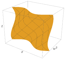
Figure 4: The string worldsheet specified by Eq. (72). The worldsheet is in effect embedded in three-dimensional spacetime $(w^{1}=0)$.

The straight lines in Fig. 4, which are geodesics, are the orbits of the null Killing vector field $k=\partialderivative*{\lambda}$. The curved lines are the orbits of the other tangent null vector field $l=\partialderivative*{\sigma}$. The worldsheet is curved along $l$, but not along $k$. This is consistent with the second fundamental form: $\quantity(K_{1})_{\sigma\sigma}=\sin\sigma\neq 0,\quantity(K_{1})_{\lambda\lambda}=0.$

V.2 The Einstein static universe

The Einstein static universe is a closed Friedmann-Lemaître-Robertson-Walker universe with a constant scale factor $a(>0)$. The metric is given by

$$\differential{s}^{2}=a^{2}\quantity[-\differential{t}^{2}+\differential{\theta}^{2}+\sin^{2}\theta\differential{\phi}^{2}+\quantity(\differential{\psi}-\cos\theta\differential{\phi})^{2}],$$ (74)

where the spatial coordinates are chosen so that they reflect the Hopf fibration of $S^{3}$. It is clear that $\partialderivative*{t}\pm\partialderivative*{\psi}$ or their constant multiples are null Killing vector fields. In order to clarify the influence of having two independent null Killing vector fields, we assume, for a while, that the scale factor $a$ is a function of $\psi-t$. Then the metric (74) admits only one null Killing vector field $k$ of the form

$$k=c\quantity(\partialderivative{t}+\partialderivative{\psi}),$$ (75)

where $c(\neq 0)$ is a constant.

For the null Killing vector field (75), the metric dual $1$-form (10) is

$$\eta=ca^{2}\quantity(-\differential{t}+\differential{\psi}-\cos\theta\differential{\phi}).$$ (76)

We readily find that

$$\rank\differential{\eta}=1,\quad\operatorname{corank}_{\mathcal{M}}\differential{\eta}=2,\quad\eta\wedge\quantity(\differential{\eta})^{1}\neq 0.$$ (77)

Then, as discussed in Subsec. II.2, the worldsheet is given as an integral manifold of the distribution $p\mapsto\ker\differential{\eta}_{p}~{}(p\in\mathcal{M})$. The following two vector fields give a basis of the kernel $\ker\differential{\eta}_{p}$ at each point $p$:

$$\partialderivative{t}-\frac{2a^{\prime}\cot\theta}{a}\partialderivative{\theta},\quad\partialderivative{\psi}+\frac{2a^{\prime}\cot\theta}{a}\partialderivative{\theta},$$ (78)

where $a^{\prime}$ is the derivative of the scale factor. In the case $a^{\prime}=0$, namely the case of the Einstein static universe, these vector fields are just $\partialderivative*{t}$ and $\partialderivative*{\psi}$, and then the worldsheet may be simply specified by $\theta,\phi=\text{const.}$

Let us obtain the worldsheet for the case $a^{\prime}\neq 0$ by applying the methods described in Subsecs. II.3 and III.2. First we take the hypersurface $t=0$ as $\Sigma_{0}$, which is transversal to the null Killing vector field $k$. Next we take coordinates $x^{1},x^{2},x^{3}$ on $\Sigma_{0}$ so that the spacetime coordinates of a point on $\Sigma_{0}$ are given by $(t,\theta,\phi,\psi)=(0,x^{1},x^{2},x^{3})$. Then the action of the $1$-parameter group of isometries $\varphi_{v}$ is given by

$$\varphi_{v}:(0,x^{1},x^{2},x^{3})\mapsto(cv,x^{1},x^{2},x^{3}+cv).$$ (79)

Let $(t,\theta,\phi,\psi)$ be the coordinates of the point $(cv,x^{1},x^{2},x^{3}+cv)$, then the coordinate transformation is given by

$$t=cv,\quad\theta=x^{1},\quad\phi=x^{2},\quad\psi=x^{3}+cv.$$ (80)

In these coordinates, the metric is written as

$$\differential{s}^{2}=2ca^{2}\quantity(\differential{x^{3}}-\cos x^{1}\differential{x^{2}})\differential{v}+a^{2}\quantity[\quantity(\differential{x^{1}})^{2}+\sin^{2}x^{1}\quantity(\differential{x}^{2})^{2}+\quantity(\differential{x^{3}}-\cos x^{1}\differential{x^{2}})^{2}],$$ (81)

where we note that the scale factor $a$ becomes a function of $x^{3}(=\psi-t)$. The metric dual $1$-form (76) is given by

$$\eta=ca^{2}\quantity(\differential{x^{3}}-\cos x^{1}\differential{x^{2}}).$$ (82)

This $1$-form is regarded as the one furnished on the hypersurface $\Sigma_{0}$ and satisfies $\eta\wedge\differential{\eta}\neq 0$. Therefore, Darboux’s theorem ensures that the hypersurface $\Sigma_{0}$ admits local coordinates $y,z,w$ such that

$$\eta=y\differential{z}+\differential{w}.$$ (83)

The coordinate transformation is, for example, given by

$$y=-ca^{2}\cos x^{1},\quad z=x^{2},\quad w=\int ca^{2}(x^{3})\differential{x^{3}}\eqqcolon f(x^{3}).$$ (84)

In these coordinates, the induced metric $h$ on $\Sigma_{0}$ is written as

$$\differential{s}_{\Sigma_{0}}^{2}=\frac{\tilde{a}^{2}}{c^{2}\tilde{a}^{4}-y^{2}}\quantity(\differential{y}-2y\frac{\tilde{a}^{\prime}}{\tilde{a}}\differential{w})^{2}+\frac{c^{2}\tilde{a}^{4}-y^{2}}{c^{2}\tilde{a}^{2}}\differential{z}^{2}+\frac{1}{c^{2}\tilde{a}^{2}}\quantity(y\differential{z}+\differential{w})^{2},$$ (85)

where $\tilde{a}$ is the function of $w$ such that $\tilde{a}(w)=a(f^{-1}(w))$, and the worldsheet is given by Eqs. (32) and (46) as

$$v(\lambda,\sigma)=\lambda+v_{0}(\sigma),\quad y(\lambda,\sigma)=y_{0},\quad z(\lambda,\sigma)=z_{0},\quad w(\lambda,\sigma)=\sigma+w_{0},$$ (86)

where $y_{0},z_{0},w_{0}$ are constants and, from Eq. (39), $v_{0}(\sigma)$ is determined as

$$v_{0}(\sigma)=-\frac{1}{2}\int h_{ww}\differential{\sigma}=-\frac{1}{2}\int\quantity(\frac{4\,y^{2}\,\tilde{a}^{\prime}{}^{2}}{c^{2}\tilde{a}^{4}-y^{2}}+\frac{1}{c^{2}\tilde{a}^{2}})\differential{\sigma}.$$ (87)

We now examine the second fundamental form of the worldsheet (86). Since the worldsheet is simply given by $y=y_{0}$ and $z=z_{0}$, we take two normal vector fields $N_{1}$ and $N_{2}$ so that their metric dual $1$-forms are $\differential{y}$ and $\differential{z}$. For these $N_{1},N_{2}$, the non-trivial components of the second fundamental form are given by Eq. (60) as

$$\quantity(K_{1})_{\sigma\sigma} =-\frac{2y_{0}}{\tilde{a}^{2}\quantity(c^{2}\tilde{a}^{4}-y_{0}^{2})^{2}}\quantity[-(c^{2}\tilde{a}^{4}-y_{0}^{2})(c^{2}\tilde{a}^{4}+2y_{0}^{2})\,\tilde{a}^{\prime}{}^{2}+4c^{2}\,y_{0}^{4}\,\tilde{a}^{2}\,\tilde{a}^{\prime}{}^{4}+(c^{2}\tilde{a}^{4}-y_{0}^{2})\,\tilde{a}\,\tilde{a}^{\prime\prime}],$$ (88)

$$\quantity(K_{2})_{\sigma\sigma} =-\frac{y_{0}\tilde{a}^{\prime}}{\tilde{a}\quantity(c^{2}\,\tilde{a}^{4}-y_{0}^{2})^{2}}\quantity[y_{0}^{2}\quantity(4c^{2}\,\tilde{a}^{2}\,\tilde{a}^{\prime}{}^{2}+1)-c^{2}\,\tilde{a}^{4}],$$ (89)

where the function $\tilde{a}$ is evaluated on the worldsheet (86), that is, $\tilde{a}=\tilde{a}(\sigma+w^{0})$. From these expressions, we readily find that if the scale factor $a$ is constant, which is the case of the Einstein static universe, the second fundamental form vanishes. Conversely, it is easily shown that if the second fundamental form of every worldsheet vanishes, the scale factor has to be constant. Therefore, the Einstein static universe is the only spacetime with the metric (74) that permits every worldsheet of null C1 symmetry to have a vanishing second fundamental form. The reason for the vanishing of the non-trivial components in the Einstein static universe is that the null vector field $l=\partialderivative*{\sigma}$ tangent to the worldsheet agrees with a constant multiple of the other null Killing vector field $\partialderivative*{t}-\partialderivative*{\psi}$: in fact, from Eqs. (86) and (87),

$$l=-\frac{1}{2c\,a^{2}}\quantity(\partialderivative{t}-\partialderivative{\psi}).$$ (90)

In the remainder of this subsection, we only consider the case $a=\text{const.}$, namely the case of the Einstein static universe, where the induced metric $h$ is given by

$$\differential{s}_{\Sigma_{0}}^{2}=\frac{a^{2}}{c^{2}a^{4}-y^{2}}\differential{y}^{2}+\frac{c^{2}a^{4}-y^{2}}{c^{2}a^{2}}\differential{z}^{2}+\frac{1}{c^{2}a^{2}}\quantity(y\differential{z}+\differential{w})^{2},$$ (91)

and the normal vector field $N_{1},N_{2}$ used above are given by

$$N_{1}=\frac{c^{2}a^{4}-y^{2}}{a^{2}}\partialderivative{y},\quad N_{2}=\frac{c^{2}a^{2}}{c^{2}a^{4}-y^{2}}\quantity(\partialderivative{z}-y\partialderivative{w}).$$ (92)

We discuss the vanishing of the second fundamental form described above from two perspectives. The first is the orthogonality of $\Sigma_{0}$ and the worldsheet $\mathcal{S}$. It follows from Eq. (92) that $\Sigma_{0}$ is orthogonal to $\mathcal{S}$, namely $g(n,N_{I})=0$, where $n$ is a unit normal vector field of $\Sigma_{0}$ given by $v=0$ in $(v,y,z,w)$ coordinates. Therefore, as discussed in Sec. IV, the vanishing of the second fundamental form implies that the curve $\mathcal{C}$, which is the section of $\mathcal{S}$ with $\Sigma_{0}$, is a geodesic on $\Sigma_{0}$. Indeed, from Eq. (86), $\mathcal{C}$ on $\Sigma_{0}$ is given by $(y(\sigma),z(\sigma),w(\sigma))=(y_{0},z_{0},\sigma+w_{0})$, and the tangent vector $\partialderivative*{w}$ is geodesic for the induced metric (91) because $\partialderivative*{w}$ is a Killing vector field of a constant norm. The second is a contact structure $(\varphi,\xi,\eta)$ on $\Sigma_{0}$. It follows from Eq. (77) that

$$\operatorname{corank}_{\Sigma_{0}}\differential{\eta}=1.$$ (93)

Thus, the hypersurface $\Sigma_{0}$ has a contact structure $(\varphi,\xi,\eta)$. As discussed in Sec. IV, a sufficient condition for the second fundamental form to vanish is that the Reeb vector field $\xi$ satisfies the geodesic equation (65), i.e., ${}^{(h)}\nabla_{\xi}\,\xi=0$. This condition is actually satisfied. In fact, in the Darboux coordinates $(y,z,w)$, the Reeb vector field $\xi$ is given by Eq. (50), i.e., $\xi=\partialderivative*{w}$ and then, is clearly a Killing vector field of a constant norm with respect to the induced metric (91). This implies that $\xi$ satisfies the geodesic equation.

We note that the induced metric $h$ given by (91) is not generally compatible with the contact structure $(\varphi,\xi,\eta)$ on $\Sigma_{0}$. However, if we set the constant $c$ of the null Killing vector field (75) to be $\pm 1/a$, the induced metric becomes compatible to $(\varphi,\xi,\eta)$, that is, $h$ satisfies

$$h(\varphi V_{1},\varphi V_{2})=h(V_{1},V_{2})-\eta(V_{1})\,\eta(V_{2})$$ (94)

for arbitrary vector fields $V_{1},V_{2}$. Indeed, if we take an orthonormal basis $\quantity{\xi_{1},\xi_{2},\xi_{3}}$ for the induced metric (91) as

$$\xi_{1}=\frac{\sqrt{a^{2}-y^{2}}}{a}\partialderivative{y},\quad\xi_{2}=\frac{1}{\sqrt{a^{2}-y^{2}}}\quantity(\partialderivative{z}-y\partialderivative{w}),\quad\xi_{3}=\xi=\partialderivative{w},$$ (95)

such that $\eta(\xi_{1})=\eta(\xi_{2})=0$, and define the $(1,1)$-tensor $\varphi$

where $\eta^{I}~{}(I=1,2,3)$ are the dual $1$-forms to $\xi_{I}$, then it is readily verified that the induced metric $h$ satisfies the compatibility condition (94).

We next examine the twist potential $\omega_{I}{}^{J}$ of the worldsheet by assuming $c=1/a$. For this aim, we have to take normal vector fields $N_{1},N_{2}$ so that they are orthonormal, namely $g(N_{I},N_{J})=\delta_{IJ}$. This requirement is satisfied by taking $\xi_{1},\xi_{2}$ of Eq. (95) to $N_{1},N_{2}$. These vector fields satisfy $\mathcal{L}_{k}N_{I}=\mathcal{L}_{l}N_{I}=0$. For these normal vector fields, Eq. (143) reads

and then, from Eq. (139), we have

$$g(\nabla_{k}N_{1},N_{2})=\frac{1}{2a},\quad g(\nabla_{l}N_{1},N_{2})=\frac{1}{4a}.$$ (96)

These equations imply that the worldsheet twists in the sense that the normal vector fields rotate when they are parallelly propagated along the null directions while the Lie derivatives vanish. We also find that for the unit timelike and spacelike vector fields tangent to the worldsheet $\mathcal{S}$

$$e_{0}\coloneqq\frac{1}{a}\partialderivative{t}=\frac{1}{2a}k-al,\quad e_{1}\coloneqq\frac{1}{a}\partialderivative{\psi}=\frac{1}{2a}k+al,$$ (97)

which are orthogonal to each other, it holds that

$$g(\nabla_{e_{0}}N_{1},N_{2})=0,\quad g(\nabla_{e_{1}}N_{1},N_{2})=\frac{1}{2a}.$$ (98)

This implies the twist of the worldsheet comes from the $e_{1}$ direction, which is the direction of the $S^{1}$ fibers in the Hopf fibration of $S^{3}$. The value $1/(2a)$ is just the half of the Hodge dual of the $3$-form $\eta\wedge\differential{\eta}$ in $\Sigma_{0}$.

V.3 The Gödel universe

We start with the following metric

$$\differential{s}^{2}=a^{2}\quantity[-\quantity(\differential{T}+e^{Y}\differential{Z})^{2}+\differential{Y}^{2}+\frac{1}{2}e^{2Y}\differential{Z}^{2}+\differential{W}^{2}],$$ (99)

where $a$ is a function of $T-W$. This metric admits a null Killing vector field $k$ of the form

$$k=c\quantity(\partialderivative{T}+\partialderivative{W}),$$ (100)

where $c$ is a constant. In the special case that $a$ is constant, the metric describes the Gödel universe and also admits another null Killing vector field given by the constant multiple of $\partialderivative*{T}-\partialderivative*{W}$.

The metric dual $1$-form of the null Killing vector field $k$ is given by

$$\eta=ca^{2}\quantity(-\differential{T}-e^{Y}\differential{Z}+\differential{W}).$$ (101)

Using the same arguments as in the previous subsection, we find that the string worldsheet is given as an integral manifold of $\ker\differential{\eta}$, which is tangent to the vector fields

$$\partialderivative{T}-2\frac{a^{\prime}}{a}\partialderivative{Y},\quad\partialderivative{W}+2\frac{a^{\prime}}{a}\partialderivative{Y}.$$ (102)

In the case that $a^{\prime}=0$, namely the case of the Gödel universe, these vector fields become $\partialderivative*{T}$ and $\partialderivative*{W}$, and then, the worldsheet can simply be given by $Y,Z=\text{const.}$

The worldsheet in the case $a^{\prime}\neq 0$ is also exactly obtained in the same way as in the previous subsection. The hypersurface $\Sigma_{0}$ is taken as $W=0$ and the spacetime coordinates $(v,x^{1},x^{2},x^{3})$ are taken so that

$$T=x^{1}+cv,\quad Y=x^{2},\quad Z=x^{3},\quad W=cv.$$ (103)

In these coordinates, the metric dual $1$-form $\eta$ is

$$\eta=-ca^{2}(x^{1})\quantity(\differential{x^{1}}+e^{x^{2}}\differential{x^{3}}).$$ (104)

It is readily found that the hypersurface $\Sigma_{0}$ admits the Darboux coordinates $y,z,w$ such that $\eta=y\differential{z}+\differential{w}$. The coordinate transformation is, for example, given by

$$y=-ca^{2}(x^{1})e^{x^{2}},\quad z=x^{3},\quad w=-c\int a^{2}(x^{1})\differential{x^{1}}\eqqcolon F(x^{1}).$$ (105)

Then, from Eqs. (32) and (46), the worldsheet is given by

$$v(\lambda,\sigma)=\lambda+v_{0}(\sigma),\quad y(\lambda,\sigma)=y_{0},\quad z(\lambda,\sigma)=z_{0},\quad w(\lambda,\sigma)=\sigma+w_{0},$$ (106)

where $y_{0},z_{0},w_{0}$ are constants and $v_{0}(\sigma)$ is a function determined by Eq. (39).

The non-trivial components of the second fundamental form are computed as

$$\quantity(K_{1})_{\sigma\sigma}=-\frac{2y\quantity[3\quantity(\tilde{a}^{\prime})^{2}+8c^{2}\tilde{a}^{2}\quantity(\tilde{a}^{\prime})^{4}+\tilde{a}\tilde{a}^{\prime\prime}]}{\tilde{a}^{2}},\quad\quantity(K_{2})_{\sigma\sigma}=\frac{2\tilde{a}^{\prime}\quantity[1+4c^{2}\tilde{a}^{2}\quantity(\tilde{a}^{\prime})^{4}]}{y\tilde{a}},$$ (107)

where $\tilde{a}$ is a function of $w$ such that $\tilde{a}(w)=a(F^{-1}(w))$. From this equation, we find that the second fundamental form vanishes if and only if $\tilde{a}$ is constant. This implies that the Gödel universe is the only spacetime with the metric (99) in which every string with a null symmetry has a vanishing second fundamental form. In the remainder of this subsection, we only consider the case that $a$ is constant, namely the case of the Gödel universe.

As we have examined so far, the string worldsheet in the Gödel universe can be discussed in the same way as in the Einstein static universe. The vanishing of the second fundamental form in the Gödel universe can also be discussed in the same way as in the previous subsection. Therefore, we will only mention the differences. The first is the squared norm of the Reeb vector field $\xi$, or equivalently the contact form $\eta$. In the Gödel universe a timelike hypersurface given by $W=0$ is taken as $\Sigma_{0}$ and the Reeb vector field $\xi$ is timelike, while in the Einstein static universe a spacelike hypersurface given by $t=0$ is taken and $\xi$ is spacelike. Therefore, we have to use the other sign of $\epsilon$ for the compatibility condition (117) in the Gödel universe. The second is the direction of the twist of the worldsheet $\mathcal{S}$. The twist potential $\omega_{I}^{J}$ is computed as

where the normal vector fields $N_{1},N_{2}$ that satisfies $g(N_{I},N_{J})=\delta_{IJ}$ are taken as

$$N_{1}=\frac{y}{a}\partialderivative{y},\quad N_{2}=\frac{\sqrt{2}}{y}\quantity(\partialderivative{z}-y\partialderivative{w}).$$ (108)

Then, it follows that

$$g(\nabla_{e_{0}}N_{1},N_{2})=\frac{1}{\sqrt{2}a},\quad g(\nabla_{e_{1}}N_{1},N_{2})=0.$$ (109)

for the unit timelike and spacelike vector fields tangent to $\mathcal{S}$:

$$e_{0}\coloneqq\frac{1}{a}\partialderivative{T}=\frac{1}{2}\partialderivative{\lambda}-\partialderivative{\sigma},\quad e_{1}\coloneqq\frac{1}{a}\partialderivative{W}=\frac{1}{2}\partialderivative{\lambda}+\partialderivative{\sigma}.$$ (110)

This result implies that the worldsheet twists along the timelike direction $\partialderivative*{T}$ in the Gödel universe while it twists along the spacelike direction $\partialderivative*{\psi}$ in the Einstein static universe. The value $1/(\sqrt{2}a)$ is also just the half of the Hodge dual of the $3$-form $\eta\wedge\differential{\eta}$ in $\Sigma_{0}$. This result is the same as in the case of the Einstein static universe.

VI Conclusion

We have investigated the dynamics of the Nambu-Goto strings with a null symmetry in curved spacetimes $\mathcal{M}$ that admit a null Killing vector field $k$. The null symmetry, or null cohomogeneity one (C1) symmetry, means that the null Killing vector field $k$ is tangent to the string worldsheet. The equation of motion and the gauge conditions are given in terms of the metric dual $1$-form $\eta\coloneqq g_{\mu\nu}k^{\mu}\differential{x^{\nu}}$. In the special case $\operatorname{corank}_{\mathcal{M}}\differential{\eta}=2$, the worldsheet is given by an integral manifold of $\ker\differential{\eta}$.

The equation of motion and the gauge conditions are generally reduced to first order ordinary differential equations on a hypersurface $\Sigma_{0}$ equipped with the $1$-form $\eta$. This $1$-form enables us to take a suitable coordinate system on the hypersurface $\Sigma_{0}$, and then it is shown that the equations are integrable.

The metric dual $1$-form $\eta$ provides the hypersurface $\Sigma_{0}$ with an almost contact structure. In the special case that $\operatorname{corank}_{\Sigma_{0}}\differential{\eta}=1$, the almost contact structure becomes a contact structure, and its Reeb vector field gives the solutions to the ordinary differential equations to be solved. That is to say, the worldsheets are completely characterized by the Reeb vector field.

We have also applied our formalism to some four-dimensional spacetimes: pp -waves in which $\differential{\eta}=0$, and the Einstein static universe and the Gödel universe in which $\differential{\eta}\neq 0$. The string worldsheets are obtained exactly and their geometries are investigated in detail.

Our work complements previous studies of C1 string dynamics, where the C1 symmetry was implicitly assumed to be non-null. It shows that a null C1 symmetry is special in the sense that the equation of motion is always integrable. For strings with a non-null C1 symmetry, the integrability requires additional spacetime symmetries such as Killing vector fields and Killing tensor fields. This point is one of the remarkable differences between null and non-null C1 symmetries.

The concept of the cohomogeneity one symmetry is extended to higher dimensional objects such as membranes [18, 19]. The application of the null cohomogeneity one symmetry to the higher dimensional objects is left for future work.

Our study reveals the existence of (almost) contact structure in the curved spacetimes that admit a null Killing vector field and its relation to the string dynamics. Applications of the (almost) contact structure to general relativity, such as the construction of solutions to the Einstein equations, may be intriguing.

Appendix A Almost contact structure

We provide an overview of the almost contact structure and related topics [30, 31].

An almost contact structure on a $(2n+1)$-dimensional manifold is characterized by a triplet $(\varphi,\xi,\eta)$, where $\varphi$ is a $(1,1)$-tensor, $\xi$ a vector field and $\eta$ a $1$-form, such that

$$\iota_{\xi}\eta=\eta(\xi)=1,$$ (111)

$$\varphi^{2}=-1+\xi\otimes\eta.$$ (112)

It is readily shown that

$$\varphi\,\xi=0,\quad\eta\circ\varphi=0,\quad\rank(\varphi)=2n.$$ (113)

We can show that any odd-dimensional manifold with a nonzero $1$-form $\eta$ admits an almost contact structure $(\varphi,\xi,\eta)$, that is, we can find $\xi,\varphi$ satisfying Eqs. (111) and (112) for a given $\eta$. First we take a vector field $\xi$ that satisfies Eq. (111). We note that the choice is not unique. Next we take $2n$ independent vector fields $\xi_{1},\dots,\xi_{2n}$ such that $\eta(\xi_{i})=0~{}(i=1,\dots,2n)$. Then we define the $(1,1)$-tensor $\varphi$ so that

$$\varphi\,\xi=0,\quad\varphi\,\xi_{2k-1}=\xi_{2k},\quad\varphi\,\xi_{2k}=-\xi_{2k-1},$$ (114)

where $k=1,\dots,n$. In this manner, we obtain an almost contact structure $(\varphi,\xi,\eta)$.

It is known that a manifold with an almost contact structure $(\varphi,\xi,\eta)$ admits a Riemannian compatible metric such that

$$h(\varphi V_{1},\varphi V_{2})=h(V_{1},V_{2})-\eta(V_{1})\,\eta(V_{2})$$ (115)

for any vector fields $V_{1}$ and $V_{2}$. Substituting $V_{1}=\xi$, we see that $\eta$ and $\xi$ are dual with respect to the compatible metric

$$\eta(V_{2})=h(\xi,V_{2}).$$ (116)

Furthermore, the norm of $\xi$ is unity; $h(\xi,\xi)=\eta(\xi)=1$. The compatible metric is generalized to the Lorentzian signature by replacing Eq. (115) with

$$h(\varphi V_{1},\varphi V_{2})=h(V_{1},V_{2})-\epsilon\eta(V_{1})\,\eta(V_{2}).$$ (117)

where $\epsilon=\pm 1$ [36]. An almost contact manifold with a compatible metric $h$ is said to have an almost contact metric structure $(\varphi,\xi,\eta,h)$.

If the compatible metric $h$ satisfies

$$h(V_{1},\varphi V_{2})=\differential{\eta}(V_{1},V_{2})$$ (118)

for any vector fields $V_{1}$ and $V_{2}$, the almost contact metric structure $(\varphi,\xi,\eta,h)$ is called a contact metric structure. In this case, it holds that

$$\eta\wedge\quantity(\differential{\eta})^{n}\neq 0,$$ (119)

where

$$\quantity(\differential{\eta})^{n}\coloneqq\underbrace{\differential{\eta}\wedge\dots\wedge\differential{\eta}}_{\text{$n$ factors}}.$$ (120)

Conversely, a $(2n+1)$-dimensional manifold furnished with a $1$-form $\eta$ satisfying Eq. (119) is said to have a contact structure. A contact manifold admits a unique vector field $\xi$ that satisfies

$$\iota_{\xi}\eta=1,\quad\iota_{\xi}\differential{\eta}=0.$$ (121)

This vector field $\xi$ is called the Reeb vector field. Hereafter, for a contact manifold, we only consider the almost contact structure $(\varphi,\xi,\eta)$ and the contact metric structure $(\varphi,\xi,\eta,h)$ such that $\xi$ is the Reeb vector field. The contact metric structure $(\varphi,\xi,\eta,h)$ is called a $K$-contact structure if the Reeb vector field $\xi$ is a Killing vector with respect to $h$.

An almost contact structure $(\varphi,\xi,\eta)$ is said to be normal if

$$\mathcal{T}_{\varphi}+2\xi\otimes\differential{\eta}=0$$ (122)

holds, where $\mathcal{T}_{\varphi}$ is a $(1,2)$-tensor called the Nijenhuis tensor defined by

$$\mathcal{T}_{\varphi}(V_{1},V_{2})\coloneqq\varphi^{2}\,\quantity[V_{1},V_{2}]+\quantity[\varphi\,V_{1},\varphi\,V_{2}]-\varphi\,\quantity[\varphi V_{1},V_{2}]-\varphi\,\quantity[V_{1},\varphi V_{2}]$$ (123)

for any vector fields $V_{1}$ and $V_{2}$. If the contact metric structure $(\varphi,\xi,\eta,h)$ is normal, the manifold is said to be a Sasakian manifold. We remark that there exist other equivalent definitions of the Sasakian manifold.

Finally, we note that for a given almost contact metric structure $(\varphi,\xi,\eta,h)$, the following $(\tilde{\varphi},\tilde{\xi},\tilde{\eta},\tilde{h})$ is also an almost contact metric structure

$$\tilde{\varphi}=\varphi,\quad\tilde{\xi}=(\lambda+\mu)^{-1/2}\xi,\quad\tilde{\eta}=(\lambda+\mu)^{1/2}\eta,\quad\tilde{h}=\lambda h+\mu\eta\otimes\eta,$$ (124)

where $\lambda,\mu$ are functions such that $\lambda>0,\lambda+\mu>0$ [37].

Appendix B Second fundamental form and twist potential

We provide an overview of the mathematical description of the worldsheet $\mathcal{S}$ viewed as a two-dimensional submanifold embedded in a $(D+1)$-dimensional spacetime $\mathcal{M}$ [38, 39]. The codimension of $\mathcal{S}$ is denoted by $\operatorname{codim}\mathcal{S}$.

Let $\mathfrak{X}(\mathcal{S})$ be the set of all tangent vector fields on $\mathcal{S}$ and $\mathfrak{X}(\mathcal{S})^{\perp}$ be that of normal vector fields on $\mathcal{S}$. The second fundamental form $\alpha$ is a symmetric map

$$\alpha:\mathfrak{X}(\mathcal{S})\times\mathfrak{X}(\mathcal{S})\to\mathfrak{X}(\mathcal{S})^{\perp}$$ (125)

such that for $X,Y\in\mathfrak{X}(\mathcal{S})$ and $p\in\mathcal{S}$,

$$\bigl{.}\alpha(X,Y)\bigr{|}_{p}=\quantity(\nabla_{X}Y)_{p}^{\perp},$$ (126)

where $\perp$ denotes the projection to the normal complement of $T_{p}\mathcal{S}$ in $T_{p}\mathcal{M}$. Then it holds that for $N\in\mathfrak{X}(\mathcal{S})^{\perp}$

$$\Bigl{.}g(N,\alpha(X,Y))\Bigr{|}_{p}=\Bigl{.}g(N,\nabla_{X}Y)\Bigr{|}_{p}.$$ (127)

Let $N_{I}~{}(I=1,\dots,\operatorname{codim}\mathcal{S})$ be normal vector fields which are independent at each point on $\mathcal{S}$. Then we express $\alpha(X,Y)$ by

$$\alpha(X,Y)=K^{I}(X,Y)\,N_{I},$$ (128)

where $K^{I}~{}(I=1,\dots,\operatorname{codim}\mathcal{S})$ are symmetric maps from $\mathfrak{X}(\mathcal{S})\times\mathfrak{X}(\mathcal{S})$ to $\mathfrak{F}(\mathcal{S})$  ($\mathfrak{F}({\mathcal{S}})$ being the set of all functions on $\mathcal{S}$). Substituting Eq. (128) to Eq. (127) with $N=N_{J}$, we have

$$g_{JI}K^{I}(X,Y)=g(N_{J},\nabla_{X}Y),$$ (129)

where $g_{JI}\coloneqq g(N_{J},N_{I})$, and then, the symmetric maps $K^{I}$ are given by

$$K^{I}(X,Y)=g^{IJ}g(N_{J},\nabla_{X}Y),$$ (130)

where $g^{IJ}$ is the inverse of $g_{IJ}$. It is more convenient to consider the symmetric map $K_{I}\coloneqq g_{IJ}K^{J}$ such that

$$K_{I}(X,Y)=g(N_{I},\nabla_{X}Y).$$ (131)

Let $\zeta^{a}~{}(a=1,2)$ be coordinates on the worldsheet $\mathcal{S}$, then the coordinate components $\quantity(K_{I})_{ab}$ are given by

$$\quantity(K_{I})_{ab}\coloneqq K_{I}(\partialderivative{\zeta^{a}},\partialderivative{\zeta^{b}})=\quantity(N_{I})_{\mu}\quantity[\partialderivative{\zeta^{a}}\quantity(\partialderivative{x^{\mu}}{\zeta^{b}})+\Gamma^{\mu}{}_{\nu\lambda}\partialderivative{x^{\nu}}{\zeta^{a}}\partialderivative{x^{\lambda}}{\zeta^{b}}].$$ (132)

Suppose that a Killing vector field $k$ of constant norm is tangent to the worldsheet. As shown in Subsec. II.2, $k$ satisfies the geodesic equation $\nabla_{k}k=0$. Therefore, it holds that $K_{I}(k,k)=0$. Taking one of the worldsheet coordinate, say $\zeta^{1}$, so that $\partialderivative*{\zeta^{1}}=k$, we obtain $\quantity(K_{I})_{11}=0$.

In terms of the symmetric maps $K_{I}$, the Nambu-Goto equation (4) reduce to

$$\Tr K_{I}\coloneqq\gamma^{ab}\quantity(K_{I})_{ab}=0,$$ (133)

where $\gamma_{ab}$ is the induced metric on $\mathcal{S}$. In fact, when we write Eq. (4) as

$$\partialderivative{\zeta^{a}}\quantity(\sqrt{-\gamma}\,\gamma^{ab})\,\partialderivative{x^{\mu}}{\zeta^{b}}+\sqrt{-\gamma}\,\gamma^{ab}\quantity[\partialderivative{\zeta^{a}}\quantity(\partialderivative{x^{\mu}}{\zeta^{b}})+\Gamma^{\mu}{}_{\nu\lambda}\partialderivative{x^{\nu}}{\zeta^{a}}\partialderivative{x^{\lambda}}{\zeta^{b}}]=0$$ (134)

and take the inner products with the normal vector fields $N_{I}$, we have

$$\gamma^{ab}\quantity(N_{I})_{\mu}\quantity[\partialderivative{\zeta^{a}}\quantity(\partialderivative{x^{\mu}}{\zeta^{b}})+\Gamma^{\mu}{}_{\nu\lambda}\partialderivative{x^{\nu}}{\zeta^{a}}\partialderivative{x^{\lambda}}{\zeta^{b}}]=\gamma^{ab}\quantity(K_{I})_{ab}=0.$$ (135)

In order to define a twist potential, we consider a map

$$\beta:\mathfrak{X}(\mathcal{S})\times\mathfrak{X}(\mathcal{S})^{\perp}\to\mathfrak{X}(\mathcal{S})^{\perp}$$ (136)

such that for $X\in\mathfrak{X}(\mathcal{S})$, $N\in\mathfrak{X}(\mathcal{S})^{\perp}$ and $p\in\mathcal{S}$

$$\Bigl{.}\beta(X,N)\Bigr{|}_{p}=\quantity(\nabla_{X}N)^{\perp}_{p}.$$ (137)

For a given set of independent normal vector fields $\quantity{N_{I}}$, we express $\beta$ by

$$\beta(X,N_{I})=\omega_{I}{}^{J}(X)N_{J},$$ (138)

where $\omega_{I}{}^{J}\quad(I,J=1,\dots,D-1)$ are maps from $\mathfrak{X}(\mathcal{S})$ to $\mathfrak{F}(\mathcal{S})$, that is, $1$-forms on $\mathcal{S}$, which are given by

$$\omega_{I}{}^{J}(X)=g(\nabla_{X}N_{I},N_{K})\,g^{KJ}.$$ (139)

When we define $1$-forms $\omega_{IJ}$ as

$$\omega_{IJ}\coloneqq g_{JJ^{\prime}}\omega_{I}{}^{J^{\prime}},$$ (140)

we can show that for any $X\in\mathfrak{X}(\mathcal{S})$

$$\omega_{IJ}(X)+\omega_{JI}(X)=X(g_{IJ}).$$ (141)

When we take another set of independent normal vector fields $G_{I}{}^{J}N_{J}\quad(G_{I}{}^{J}\in\mathrm{GL}(D-1))$, the maps $\omega_{I}{}^{J}$ are transformed as

$$\quantity(\omega_{I}{}^{J})_{a}\mapsto G_{I}{}^{I^{\prime}}\,\quantity(\omega_{I^{\prime}}{}^{J^{\prime}})_{a}\quantity(G^{-1})_{J^{\prime}}{}^{J}+\partialderivative{\zeta^{a}}\quantity(G_{I}{}^{I^{\prime}})\quantity(G^{-1})_{I^{\prime}}{}^{J},$$ (142)

where $\quantity(\omega_{I}{}^{J})_{a}$ are the coordinate components

$$\quantity(\omega_{I}{}^{J})_{a}\coloneqq\omega_{I}{}^{J}(\partialderivative{\zeta^{a}})=g_{\mu\nu}\quantity[\partialderivative{\quantity(N_{I})^{\mu}}{\zeta^{a}}+\Gamma^{\mu}{}_{\alpha\beta}\,\partialderivative{x^{\alpha}}{\zeta^{a}}\quantity(N_{I})^{\beta}]\quantity(N_{K})^{\nu}g^{KJ}.$$ (143)

Since $\quantity(\omega_{I}{}^{J})_{a}$ transforms as a connection, we can define the curvature $2$-forms $\Omega_{I}{}^{J}$ associated with $\omega_{I}{}^{J}$ as

$$\Omega_{I}{}^{J}=\differential{\omega}_{I}{}^{J}+\omega_{I}{}^{K}\wedge\omega_{K}{}^{J}.$$ (144)

The coordinate components are given by

$$\quantity(\Omega_{I}{}^{J})_{ab}\coloneqq D_{a}\quantity(\omega_{I}{}^{J})_{b}-D_{b}\quantity(\omega_{I}{}^{J})_{a}+\quantity(\omega_{I}{}^{K})_{a}\quantity(\omega_{K}{}^{J})_{b}-\quantity(\omega_{I}{}^{K})_{b}\quantity(\omega_{K}{}^{J})_{a},$$ (145)

where $D_{a}$ denotes the covariant derivative on $\mathcal{S}$.

When we impose independent normal vector fields $N_{I}$ to be orthonormal, that is $g_{IJ}=g(N_{I},N_{J})=\delta_{IJ}$, it follows from Eq. (141) that $\omega_{IJ}$ are antisymmetric with respect to the indices $I,J$, and the maps $\omega_{I}{}^{J}$ are called the (extrinsic) twist potential.

Appendix C Derivation of Eq. (60)

The orthogonal projection $P_{n}:T_{p}\mathcal{M}\to T_{p}\Sigma_{0}$ is given by

$$\quantity(P_{n})^{\mu}{}_{\nu}=\delta^{\mu}{}_{\nu}-\epsilon\,n^{\mu}n_{\nu},\quad\epsilon=\begin{cases}1&\text{for $g(n,n)=1$}\\ -1&\text{for $g(n,n)=-1$}\end{cases}.$$ (146)

Then a vector $X\in T_{p}\mathcal{M}$ is decomposed as

$$X=\epsilon g(n,X)n+P_{n}X.$$ (147)

The null Killing vector $k$ is also decomposed as

$$k=\epsilon g(n,k)n+P_{n}k$$ (148)

and hence, the unit vector $n$ perpendicular to the hypersurface $\Sigma_{0}$ is given by

$$n=\frac{1}{\epsilon g(n,k)}\quantity(k-P_{n}k).$$ (149)

Substituting this equation into Eq. (147), we have

$$X=\frac{g(n,X)}{g(n,k)}k+P_{n}X-\frac{g(n,X)}{g(n,k)}P_{n}k.$$ (150)

This equation gives the projection $P_{k}:T_{p}\mathcal{M}\to T_{p}\Sigma_{0}$ along $k$ so that

$$P_{k}X=P_{n}X-\frac{g(n,X)}{g(n,k)}P_{n}k\quad\text{or}\quad P_{k}X=X-\frac{g(n,X)}{g(n,k)}k.$$ (151)

Eqs. (148) and (151), give the following formula that plays an important role in deriving Eq. (60)

$$g(P_{k}X,P_{k}Y)=g(P_{k}X,P_{n}Y)\quad\text{for $X,Y\in T_{p}\mathcal{M},\quad g(X,k)=0$}.$$ (152)

Now we derive Eq. (60). First we observe that, for $\hat{l}\coloneqq P_{k}l$,

$$K_{I}(\hat{l},\hat{l})=K_{I}(l,l)\eqqcolon\quantity(K_{I})_{\sigma\sigma},$$ (153)

where we have used Eq. (54) and (55). Then, from Eq. (53), $\quantity(K_{I})_{\sigma\sigma}$ is given by

$$\quantity(K_{I})_{\sigma\sigma}=g(N_{I},\nabla_{\hat{l}}\,\hat{l}\,).$$ (154)

Next, we decompose $N_{I}$ and $\nabla_{\hat{l}}\,\hat{l}$ by using Eq. (151). Then Eq. (154) leads to

$$\quantity(K_{I})_{\sigma\sigma}=g(P_{k}N_{I},P_{k}\nabla_{\hat{l}}\,\hat{l}).$$ (155)

In the process of the derivation, we have used the equations $\nabla_{k}k=0$, $\nabla_{l}k=0$ and $g(k,l)=1$, which are different expressions of Eqs. (13), (15) and (30) respectively. Finally, using the formula (152), we obtain

$$\quantity(K_{I})_{\sigma\sigma}=g(P_{k}N_{I},P_{n}\nabla_{\hat{l}}\,\hat{l}\,).$$ (156)

References

- Vilenkin and Shellard [2000] A. Vilenkin and E. P. S. Shellard, Cosmic Strings and Other Topological Defects (Cambridge University Press, 2000).
- Polchinski [1998] J. Polchinski, String Theory (Cambridge University Press, 1998).
- Ishihara and Kozaki [2005] H. Ishihara and H. Kozaki, Phys. Rev. D 72, 061701(R) (2005), arXiv:gr-qc/0506018 .
- Frolov et al. [1989] V. P. Frolov, V. Skarzhinsky, A. Zelnikov, and O. Heinrich, Phys. Lett. B 224, 255 (1989).
- Carter and Frolov [1989] B. Carter and V. P. Frolov, Class. Quant. Grav. 6, 569 (1989).
- Kinoshita et al. [2016] S. Kinoshita, T. Igata, and K. Tanabe, Phys. Rev. D 94, 124039 (2016), arXiv:1610.08006 [gr-qc] .
- Boos and Frolov [2018] J. Boos and V. P. Frolov, Phys. Rev. D 97, 084015 (2018), arXiv:1801.00122 [gr-qc] .
- Igata et al. [2018] T. Igata, H. Ishihara, M. Tsuchiya, and C.-M. Yoo, Phys. Rev. D 98, 064021 (2018), arXiv:1806.09837 [gr-qc] .
- Pando Zayas and Terrero-Escalante [2010] L. A. Pando Zayas and C. A. Terrero-Escalante, JHEP 09, 094, arXiv:1007.0277 [hep-th] .
- Basu et al. [2011] P. Basu, D. Das, and A. Ghosh, Phys. Lett. B 699, 388 (2011), arXiv:1103.4101 [hep-th] .
- Ishii et al. [2017] T. Ishii, K. Murata, and K. Yoshida, Phys. Rev. D 95, 066019 (2017), arXiv:1610.05833 [hep-th] .
- Basu and Pando Zayas [2011a] P. Basu and L. A. Pando Zayas, Phys. Lett. B 700, 243 (2011a), arXiv:1103.4107 [hep-th] .
- Basu and Pando Zayas [2011b] P. Basu and L. A. Pando Zayas, Phys. Rev. D 84, 046006 (2011b), arXiv:1105.2540 [hep-th] .
- Asano et al. [2015] Y. Asano, D. Kawai, H. Kyono, and K. Yoshida, JHEP 08, 060, arXiv:1505.07583 [hep-th] .
- Rigatos [2020] K. S. Rigatos, Phys. Rev. D 102, 106022 (2020), arXiv:2009.11878 [hep-th] .
- Koike et al. [2008] T. Koike, H. Kozaki, and H. Ishihara, Phys. Rev. D 77, 125003 (2008), arXiv:0804.0084 [gr-qc] .
- Ida [2020] D. Ida, J. Math. Phys. 61, 082501 (2020), arXiv:2003.06666 [math-ph] .
- Kozaki et al. [2015] H. Kozaki, T. Koike, and H. Ishihara, Phys. Rev. D 91, 025007 (2015), arXiv:1410.6580 [gr-qc] .
- Hasegawa and Ida [2018] M. Hasegawa and D. Ida, Phys. Rev. D 98, 084003 (2018), arXiv:1808.06065 [gr-qc] .
- Morisawa et al. [2019] Y. Morisawa, S. Hasegawa, T. Koike, and H. Ishihara, Class. Quant. Grav. 36, 155009 (2019), arXiv:1709.07659 [hep-th] .
- Kozaki et al. [2010] H. Kozaki, T. Koike, and H. Ishihara, Class. Quant. Grav. 27, 105006 (2010), arXiv:0907.2273 [gr-qc] .
- Amati and Klimcik [1988] D. Amati and C. Klimcik, Phys. Lett. B 210, 92 (1988).
- Horowitz and Steif [1990] G. T. Horowitz and A. R. Steif, Phys. Rev. Lett. 64, 260 (1990).
- de Vega and Sanchez [1990a] H. J. de Vega and N. G. Sanchez, Phys. Rev. Lett. 65, 1517 (1990a).
- de Vega and Sanchez [1990b] H. J. de Vega and N. G. Sanchez, Phys. Lett. B 244, 215 (1990b).
- Arnold [1989] V. I. Arnold, Mathematical methods of classical mechanics 2nd ed. (Springer, 1989).
- Mrugala et al. [1991] R. Mrugala, J. D. Nulton, J. Christian Schön, and P. Salamon, Reports on Mathematical Physics 29, 109 (1991).
- Rajeev [2008] S. G. Rajeev, Annals Phys. 323, 2265 (2008), arXiv:0711.4319 [hep-th] .
- Dahl [2004] M. Dahl, Progress In Electromagnetics Research 46, 77 (2004).
- Sasaki [1960] S. Sasaki, Tohoku Mathematical Journal, Second Series 12, 459 (1960).
- Blair [1976] D. E. Blair, Contact manifolds in Riemannian geometry (Springer, 1976).
- Gauntlett et al. [2004] J. P. Gauntlett, D. Martelli, J. Sparks, and D. Waldram, Adv. Theor. Math. Phys. 8, 711 (2004), arXiv:hep-th/0403002 .
- Ishihara and Matsuno [2022a] H. Ishihara and S. Matsuno, PTEP 2022, 013E02 (2022a), arXiv:2109.11740 [hep-th] .
- Ishihara and Matsuno [2022b] H. Ishihara and S. Matsuno, PTEP 2022, 023E01 (2022b), arXiv:2112.02782 [hep-th] .
- Stephani et al. [2003] H. Stephani, D. Kramer, M. MacCallum, C. Hoenselaers, and E. Herlt, Exact solutions of Einstein’s field equations, 2nd ed. (Cambridge University Press, 2003).
- Calvaruso and Perrone [2010] G. Calvaruso and D. Perrone, Differential Geom. Appl. 28, 615 (2010).
- Alexiev and Ganchev [1986] V. A. Alexiev and G. T. Ganchev, C. R. Acad. Bulgare Sci. 39, 27 (1986).
- Kobayashi and Nomizu [1969] S. Kobayashi and K. Nomizu, Foundations of differential geometry, Vol. 2 (Wiley, 1969).
- Capovilla and Guven [1995] R. Capovilla and J. Guven, Phys. Rev. D 51, 6736 (1995), arXiv:gr-qc/9411060 .