Equilibriums of extremely magnetized compact stars with force-free magnetotunnels

Abstract

We present numerical solutions for stationary and axisymmetric equilibriums of compact stars associated with extremely strong magnetic fields. The interior of the compact stars is assumed to satisfy ideal magnetohydrodynamic (MHD) conditions, while in the region of negligible mass density the force-free conditions or electromagnetic vacuum are assumed. Solving all components of Einstein’s equations, Maxwell’s equations, ideal MHD equations, and force-free conditions, equilibriums of rotating compact stars associated with mixed poloidal and toroidal magnetic fields are obtained. It is found that in the extreme cases the strong mixed magnetic fields concentrating in a toroidal region near the equatorial surface expel the matter and form a force-free toroidal magnetotunnel. We also introduce a new differential rotation law for computing solutions associated with force-free magnetosphere, and present other extreme models without the magnetotunnel.

I Introduction

Models for magnetars or hyper massive remnants of binary neutron star mergers are considered to be associated with strong magnetic fields around $10^{14}$–$10^{15}$G at their surfaces Magnetar ; Magnetar_review . Such strong magnetic fields plays essential roles in generating the signals arriving from the Soft Gamma Repeater and anomalous X-ray pulsar, as well as the jet of the merger remnants. These magnetic fields are stronger than any other observed objects, and their interior magnetic fields could be one or two orders of magnitude stronger. It is, however, far too weak to modify the equilibrium structure of the compact stars. Therefore in a theoretical modeling of such compact stars, the electromagnetic fields may be treated as a perturbation, and hence separately from the hydrostatic equilibriums of the stars (see e.g. PolTorMS ; Tsokaros:2021tsu ).

Although it may be astrophysically unrealistic in the present universe, it is theoretically interesting to further investigate the compact stars associated with extremely strong magnetic fields – strong enough to modify the configuration of equilibrium structure and to dominate as a source of gravity. It is also interesting theoretically to study the strongest limit of magnetic fields of the compact star. Such solutions may be of use for initial data sets for simulations MRNSsimulations from which the behavior of magnetic fields of compact stars would be elucidated within a relatively short simulation time Tsokaros:2021pkh .

In our previous papers Uryu:2014tda ; Uryu:2019ckz , we have developed a numerical code for stationary and axisymmetric equilibriums of relativistic rotating stars associated with extremely strong electromagnetic fields based on our versatile code library, cocal (Compact Object CALculator), for calculating equilibriums and quasi-equilibrium initial data cocal . In this code, a full set of Einstein-Maxwell equations accompanied with ideal MHD equations are solved under assumptions of stationarity and axisymmetry consistently for the first time. In the paper Uryu:2019ckz (hereafter Paper I), we have obtained solutions with mixed poloidal and toroidal magnetic fields whose exteriors are electromagnetic vacuum. We demonstrated that in the extreme cases the matter in a toroidal region near the equatorial surface was partly expelled by the extremely strong magnetic fields. Such solutions have been used as initial data for fully numerical relativity simulations in Tsokaros:2021pkh .

In this paper, we introduce two new extensions to our previous works Uryu:2014tda ; Uryu:2019ckz , one is the force-free magnetic fields, and the other is the differential rotation. In paper I, we assumed electromagnetic vacuum in the region where the energy density of the matter (or the rest mass density) became negligible following the idea of Bocquet:1995je . The former extension is introduced to replace the electromagnetic vacuum with the force-free electromagnetic plasma region. Such low density regions appear not only at the exterior of the surface of a compact star, but also is expected to appear in the interior of it when the magnetic fields are stronger than the above mentioned solutions obtained in previous Paper I. To realize this, we follow a prescription for computing such compact stars associated with magnetosphere proposed by Southampton group Glampedakis:2013kaa . This prescription has been also investigated by Florence group Pili:2014zna for computing relativistic non-rotating stars under a simplified spatially conformal flat metric for the strong gravity (for numerical computations of magnetized relativistic stars, see also, Bocquet:1995je ; MRNSequilibriums ). As we will see below, in the newly calculated solutions, it is found that the mixed poloidal and toroidal magnetic fields concentrate near, but well inside of, the equatorial surface, and that the fields totally expel the matter there, when the field strength becomes of the order of $10^{17}$G or higher for typical neutron stars, that is, a toroidal force-free magnetotunnel is formed in such a solution. We also calculated the solutions replacing the electromagnetic vacuum exterior with the force-free magnetosphere. The latter extension for introducing the differential rotation is used to compute a rotating magnetized compact stars surrounded by the magnetosphere. For a comparison, differentially rotating models with electromagnetic vacuum exterior are also obtained.

This paper is organized as follows. In Sec. II, we formulate the force-free fields in terms of variables used in our previous works Uryu:2014tda ; Uryu:2019ckz , and then introduce details of the formulation adapted to the numerical method. In Sec. III, new numerical solutions combining the force-free fields, differential rotations, as well as the electromagnetic vacuum as in the previous paper are presented.

II Formulation and numerical method for the force-free electromagnetic fields

In Paper I, we have detailed the formulation and numerical method for computing stationary and axisymmetric equilibriums of strongly magnetized relativistic rotating stars. A set of equations to be solved includes the rest mass conservation equation, ideal MHD conditions, MHD-Euler equations associated with the barotropic equation of state, and the magnetic and gravitational field equations. From the consistency of the set of ideal MHD equations under the stationarity and axisymmetry, a set of integrability conditions and first integrals are derived. In particular, it requires an existence of a master potential $\Upsilon$ that several quantities (as well as combinations of quantities), for example, the $t$ and $\phi$ components of the electromagnetic 1-form $A_{\alpha}$ are the function of $\Upsilon$, $A_{t}=A_{t}(\Upsilon)$, $A_{\phi}=A_{\phi}(\Upsilon)$.

To obtain solutions in Paper I, we assumed that the star is ideal MHD fluid, and furthermore that the outside of the star is electromagnetic vacuum. Because the above dependences $A_{t}=A_{t}(\Upsilon)$ and $A_{\phi}=A_{\phi}(\Upsilon)$ are valid only on the support of ideal MHD fluid, the $A_{t}$ and $A_{\phi}$ components should be solved independently from Maxwell’s equations in the electromagnetic vacuum region, although the latter assumption may not be astrophysically realistic.

In this work, we introduce an option to replace the assumption for the electromagnetic vacuum with the force-free electromagnetic fields in the low density region out of the ideal MHD region. We introduce below the formulation for the force-free electromagnetic fields which is adapted to our formulation for magnetized compact stars in Paper I. It turns out that only a minor modification is necessary to implement the force-free formulation into our previously developed code Uryu:2019ckz .

Hereafter, we use abstract index notation for tensors; the Greek letters $\alpha,\beta,\gamma,...$ stand for 4D objects, the Latin lowercase letters $a,b,c,...$ for spatial 3D objects, and the Latin uppercase letters $A,B,C,...$ for meridional 2D objects. Also, we sometimes express the 2-forms, $F,dA$, and $d(h{\underline{u}})$ omitting indices. Such index-free notation may be used, with caution, for calculations involving forms and vectors. A dot denotes an inner product, that is, a contraction between adjacent indices. For example, a vector $v$ and a $p$-form $\omega$ have inner product

$$v\cdot\omega=v^{\gamma}\omega_{\gamma\alpha\dots\beta},\quad\omega\cdot v=\omega_{\alpha\dots\beta\gamma}v^{\gamma}.$$ (1)

We introduce 3+1 form of the spacetime metric with conformally decomposed spatial metric,

$$ds^{2}=-\alpha^{2}dt^{2}+\psi^{4}\tilde{\gamma}_{ab}(dx^{a}+\beta^{a}dt)(dx^{b}+\beta^{b}dt)$$ (2)

where $\alpha$, $\beta^{a}$, $\psi$, and $\tilde{\gamma}_{ab}$ are the lapse, the shift, the conformal factor, and the conformally related spatial metric, respectively. The $\tilde{\gamma}_{ab}$ is further decomposed with the reference 3D flat metric $f_{ab}$ as $\tilde{\gamma}_{ab}=f_{ab}+h_{ab}$, and the conformal decomposition is constrained by a condition $\tilde{\gamma}=f$ where $\tilde{\gamma}$ and $f$ are the determinant of $\tilde{\gamma}_{ab}$ and $f_{ab}$, respectively. We further assume the spacetime is asymptotically flat and impose the Dirac gauge and the maximal slicing conditions as coordinate conditions.

Further details in notations and a common part of formulations are found in Paper I.

II.1 Force-free condition

We assume stationarity and axisymmetry associated, respectively, with the timelike and spacelike Killing vectors $t^{\alpha}$ and $\phi^{\alpha}$. These vectors are used as basis of vector and tensor quantities, for example, the current vector $j^{\alpha}$ may be written

$$j^{\alpha}=j^{t}t^{\alpha}+j^{\phi}\phi^{\alpha}+j^{A}e_{A}^{\alpha},$$ (3)

where $e_{A}^{\alpha}$ are the coordinate basis of the other two spatial coordinates $x^{A}$, such as $r$ and $\theta$.

We assume that in the exterior of the ideal MHD fluid, the force-free electromagnetic field is carried by a certain plasma current whose density is negligible. Each component of the force-free conditions $F\cdot j=F_{{\alpha\beta}}j^{\beta}=0$ in stationary and axisymmetric system becomes as follows:
$t$-component:

$$t\cdot(F\cdot j) = t\cdot(F\cdot e_{A})j^{A}=j^{A}F_{tA}$$ (4)

$$= -j^{A}\partial_{A}A_{t}=0,$$

$\phi$-component:

$$\phi\cdot(F\cdot j) = \phi\cdot(F\cdot e_{A})j^{A}=j^{A}F_{\phi A}$$ (5)

$$= -j^{A}\partial_{A}A_{\phi}=0,$$

$x^{A}$-components:

$$e_{A}\cdot(F\cdot j)=e_{A}\cdot(F\cdot t)j^{t}+e_{A}\cdot(F\cdot\phi)j^{\phi}$$

$$\qquad\qquad\quad\ +e_{A}\cdot(F\cdot e_{B})j^{B}$$

$$\qquad\quad=F_{At}j^{t}+F_{A\phi}j^{\phi}+F_{AB}j^{B}$$

$$\qquad\quad=j^{t}\partial_{A}A_{t}+j^{\phi}\partial_{A}A_{\phi}+(dA)_{AB}j^{B}=0.\ \$$ (6)

The $x^{A}$ components of Maxwell’s equations are written,

$$4\pi j^{A}\sqrt{-g}\,=\,\partial_{B}(F^{AB}\sqrt{-g})\,=\,\epsilon^{AB}\partial_{B}(\sqrt{-g}B),$$ (7)

where $B$ is defined as $F^{AB}=\epsilon^{AB}B$ (see, Sec.II.F.3 of Paper I).

Substituting Eq. (7) to $t$ and $\phi$ components of the force-free conditions Eqs. (4) and (5), we have,

$$\epsilon^{AB}\partial_{A}A_{t}\,\partial_{B}(\sqrt{-g}B)=0,$$ (8)

$$\epsilon^{AB}\partial_{A}A_{\phi}\,\partial_{B}(\sqrt{-g}B)=0.$$ (9)

Hence, similarly to the case with ideal MHD fluid, the integrability conditions for the region of force-free electromagnetic fields can be written in terms of the master potential $\Upsilon$,

$$A_{t}=A_{t}(\Upsilon),\quad\ \ A_{\phi}=A_{\phi}(\Upsilon),$$

$$\!\!\!\!\!\!\!\!\!\!\!\!\!\!\!\!\!\!\mbox{and}\qquad\quad\sqrt{-g}B=[\,\sqrt{-g}B\,](\Upsilon).$$ (10)

Substituting the meridional component of the current ($x^{A}$ component of the Maxwell’s equations) (7) and a definition $F_{AB}=\epsilon_{AB}B_{\phi}$, the $x^{A}$ component of the force-free condition (6) becomes

$$j^{t}\sqrt{-g}\partial_{A}A_{t}\,+\,j^{\phi}\sqrt{-g}\partial_{A}A_{\phi}\,-\,\frac{1}{4\pi}B_{\phi}\partial_{A}[\sqrt{-g}B]\,=\,0.$$ (11)

The conditions (10) imply

$$\left(A^{\prime}_{t}j^{t}\sqrt{-g}\,+\,A^{\prime}_{\phi}j^{\phi}\sqrt{-g}\,-\,\frac{1}{4\pi}[\sqrt{-g}B]^{\prime}B_{\phi}\,\right)\partial_{A}\Upsilon=0,$$ (12)

where the primes $A^{\prime}_{t}$, $A^{\prime}_{\phi}$ and $[\sqrt{-g}B]^{\prime}$ stands for a derivative with respect to the master potential $\Upsilon$. Therefore, we have a consistency relation, which we also call first integral, for the stationary and axisymmetric force-free fields to satisfy,

$$A^{\prime}_{t}j^{t}\sqrt{-g}\,+\,A^{\prime}_{\phi}j^{\phi}\sqrt{-g}\,-\,\frac{1}{4\pi}[\sqrt{-g}B]^{\prime}B_{\phi}=0.$$ (13)

The $t$ and $\phi$ components of Maxwell’s equations are written, respectively

$$4\pi j^{t}\sqrt{-g} = \partial_{A}(F^{tA}\sqrt{-g}),$$ (14)

$$4\pi j^{\phi}\sqrt{-g} = \partial_{A}(F^{\phi A}\sqrt{-g}).$$ (15)

Substituting either (14) or (15) to Eq. (13), we have a relation for $j^{\phi}$ or $j^{t}$ to be used as a source term for an equation to determine the master potential, which is related to either $A_{\phi}(\Upsilon)$ or $A_{t}(\Upsilon)$, respectively. So far in our actual numerical computations, we have been always choosing the master potential to be $\Upsilon=A_{\phi}$, and hence $\phi$ component of Maxwell’s equations is used to determine the potential $A_{\phi}$ (see, Paper I).

II.2 A model of Force-free field around an ideal MHD region

In our formulation of ideal MHD presented in Paper I, we explicitly use the current $j^{\alpha}$ as an intermediate variable. Analogously, we have written down in the previous section II.1 the force-free conditions as Eqs.(10) and (13), whose forms are similar to the ideal MHD conditions, $F.u=0$. In actual computations, we choose $A_{\phi}$ as a master potential, $\Upsilon=A_{\phi}$. Then, the integrability conditions and relations involves the current are written,

$$A_{t}\,=\,A_{t}(A_{\phi})\quad\mbox{and}\quad\sqrt{-g}B\,=\,[\,\sqrt{-g}B\,](A_{\phi}),\quad$$ (16)

$$\qquad j^{A}\sqrt{-g}\,=\,\frac{1}{4\pi}[\sqrt{-g}B]^{\prime}\delta^{AB}B_{B},$$ (17)

$$\qquad j^{\phi}\sqrt{-g}\,+\,A^{\prime}_{t}j^{t}\sqrt{-g}\,=\,\frac{1}{4\pi}[\sqrt{-g}B]^{\prime}B_{\phi}.$$ (18)

where $B_{A}$ is defined by $\partial_{A}A_{\phi}=-\epsilon_{A}{}^{B}B_{B}$, $\delta^{AB}$ is the Kronecker delta.

The corresponding expressions for the components of the current for ideal MHD fluid are (see, Eqs. (135) and (136) of Paper I),

$$j^{A}\sqrt{-g}\,=\,\left([\sqrt{-g}\Psi]^{\prime\prime}hu_{\phi}+[\sqrt{-g}\Lambda_{\phi}]^{\prime}\right)\delta^{AB}B_{B}$$

$$\qquad\qquad\,-\,[\sqrt{-g}\Psi]^{\prime}\delta^{AB}\omega_{B},$$ (19)

$$j^{\phi}\sqrt{-g}\,+\,A^{\prime}_{t}\,j^{t}\sqrt{-g}$$

$$\quad\,=\,\left([\sqrt{-g}\Psi]^{\prime\prime}hu_{\phi}+[\sqrt{-g}\Lambda_{\phi}]^{\prime}\right)B_{\phi}\,-\,[\sqrt{-g}\Psi]^{\prime}\omega_{\phi}$$

$$\quad\,-\,\left(A^{\prime\prime}_{t}\,hu_{\phi}+\Lambda^{\prime}\right)\rho u^{t}\sqrt{-g}\,-\,s^{\prime}T\rho\sqrt{-g},$$ (20)

where arbitrary functions $\sqrt{-g}\Lambda_{\phi}$ and $\Lambda$, the stream function $\sqrt{-g}\Psi$, and the entropy per baryon mass $s$ are functions of the master potential $A_{\phi}$

$$\sqrt{-g}\Lambda_{\phi}=[\sqrt{-g}\Lambda_{\phi}](A_{\phi}),\quad\ \Lambda=\Lambda(A_{\phi}),$$

$$\!\!\sqrt{-g}\Psi=[\sqrt{-g}\Psi](A_{\phi}),\quad\mbox{and}\quad s=s(A_{\phi}).$$ (21)

In Eqs. (19) and (20), the terms including the stream functions $\sqrt{-g}\Psi$ are related to the meridional flow fields, $\rho$ is the rest mass density and $T$ the temperature. Since near the surface of compact stars, $\rho\rightarrow 0$, and $[\sqrt{-g}\Psi]\rightarrow\mbox{constant}$, terms related to the fluid approach to zero, and hence the remaining terms are

$$j^{A}\sqrt{-g}\,\rightarrow\,[\sqrt{-g}\Lambda_{\phi}]^{\prime}\delta^{AB}B_{B}$$ (22)

$$j^{\phi}\sqrt{-g}\,+\,A^{\prime}_{t}\,j^{t}\sqrt{-g}\,\rightarrow\,[\sqrt{-g}\Lambda_{\phi}]^{\prime}B_{\phi}$$ (23)

Therefore, comparing (17), (18) and (22), (23), we can smoothly connect the expressions of the current in the ideal MHD fluid region and in the force-free magnetosphere with the negligible density by choosing a common arbitrary function satisfying

$$\frac{1}{4\pi}[\sqrt{-g}B]^{\prime}=[\sqrt{-g}\Lambda_{\phi}]^{\prime},$$ (24)

in the whole domain of computation, and therefore connect the electromagnetic fields smoothly.

II.3 Construction of magnetized star with magnetosphere/magnetotunnel

As mentioned earlier, in the previous Paper I following Bocquet:1995je , a region outside of the compact star was assumed to be the electromagnetic vacuum where the electric current vanishes. Therefore, a component of vector potential $A_{t}$ was a function of $A_{\phi}$ on the ideal MHD fluid support, but was independent of $A_{\phi}$ otherwise. Assuming $A_{\phi}$ to be smooth across the stellar surface, we introduced (implicitly) the surface charge for $A_{t}$ to be continuous, but its normal derivative at the surface to be discontinuous. Such a solution can be computed by adding a homogeneous function in solving $A_{t}$ to satisfy the above conditions at the surface.

In our formulation for the force-free magnetosphere/magnetotunnel, we assume that the component $A_{t}$ is a function of $A_{\phi}$ in the whole domain and that a conducting current flows continuously and smoothly across the stellar surface. Therefore, $A_{t}$ is no longer solved independently in the outside of the ideal MHD region. As it has been found in Paper I, when the toroidal magnetic field becomes extremely strong, the mixed poloidal and toroidal magnetic fields concentrate near the equatorial surface, and they expel the high density matter of compact stars. It was, and, so far, it is not possible for the cocal code to compute a toroidal vacuum tunnel inside of the compact star, because a method to impose a boundary condition to compute $A_{t}$ for such a toroidal region has not been developed yet. On the other hand, if we assume a force-free field in such a toroidal region, the force-free magnetotunnel where the matter is expelled totally can be calculated straightforwardly under the above mentioned assumption in the same manner as computing the magnetosphere outside of the compact star. In latter sections, we will present such compact stars contain the magnetotunnel inside.

II.3.1 Formulation for the fluid variables in equilibrium

An equilibrium solution of the magnetized compact star can be calculated from a system of first integrals and integrability conditions derived in Paper I. For choices with $\Upsilon=A_{\phi}$, and without meridional flows $[\sqrt{-g}\Psi](\Upsilon)=\mbox{constant}$, the following relations obtained from the normalization condition of 4-velocity $u\cdot u=-1$, ideal MHD condition, and MHD-Euler equation (see, Paper I Sec.III.C),

$$u^{t} = \frac{1}{\left[\alpha^{2}-\psi^{4}\tilde{\gamma}_{ab}(v^{a}+\beta^{a})(v^{b}+\beta^{b})\right]^{1/2}},$$ (25)

$$\frac{u^{\phi}}{u^{t}} = -A^{\prime}_{t}\,=\,\Omega,$$ (26)

$$h\, = \frac{\Lambda}{u_{t}-A^{\prime}_{t}u_{\phi}},$$ (27)

where the angular velocity of the matter $\Omega$ is also an arbitrary function of $A_{\phi}$ (Ferraro’s law),

$$\Omega=\Omega(A_{\phi}),$$ (28)

and the 4-velocity is written,

$$u^{\alpha}\,=\,u^{t}(t^{\alpha}+v^{\alpha})\,=\,u^{t}(t^{\alpha}+\Omega\phi^{\alpha}),$$ (29)

because the meridional components $u^{A}$ is assumed to vanish $u^{A}=u^{t}v^{A}=0$.

II.3.2 Choice for arbitrary functions

Further assuming the homentropic flow $s=\mbox{constant}$, five arbitrary functions of $A_{\phi}$,

$$\qquad A_{t}(A_{\phi}),\ \ \Omega(A_{\phi}),\ \ \Lambda(A_{\phi}),$$

(30)

$$[\sqrt{-g}\Lambda_{\phi}](A_{\phi}),\ \ \mbox{and}\ \ [\sqrt{-g}B](A_{\phi}),$$

appear in the above formulation for the matter (25)–(27) and the current (17)–(20). Because of the assumption (24), four arbitrary functions remain to be specified.

For some arbitrary functions above, we choose, as in Paper I, a two parameter sigmoid function $\Xi^{\prime}(x;b,c)$ that varies from $0$ to $1$ in between $0<x<1$

$$\Xi^{\prime}(x;b,c)=\frac{1}{2}\left[\,\tanh\left(\frac{x}{b}-c\right)+1\,\right],$$ (31)

where $b$ $(0<b<1)$ is a parameter for the transition width, and $c$ $(0<c<1)$ for the transition center. Also, its integral $\Xi(x;b,c)$ becomes

$$\Xi(x;b,c)=\frac{1}{2}\left[\,b\,\ln\cosh\left(\frac{x}{b}-c\right)+x\,\right]+{\rm constant}.$$ (32)

In actual computations, functions $\Xi^{\prime}(A_{\phi})$ and $\Xi(A_{\phi})$ are defined by

$$\Xi^{\prime}(A_{\phi})=\frac{1}{2}\left[\,\tanh\left(\frac{1}{b}\frac{A_{\phi}-A_{\phi}^{0}}{A_{\phi}^{1}-A_{\phi}^{0}}-c\right)+1\,\right],$$ (33)

and

$$\Xi(A_{\phi})\,=\,\frac{1}{2}\left[\,b(A_{\phi}^{1}-A_{\phi}^{0})\times\phantom{\frac{1}{b}}\right.$$

$$\ \ \left.\ln\cosh\left(\frac{1}{b}\frac{A_{\phi}-A_{\phi}^{0}}{A_{\phi}^{1}-A_{\phi}^{0}}-c\right)+A_{\phi}\,\right]+{\rm constant},\qquad$$ (34)

where the constant of Eq. (34) is set to be $\Xi(-\infty)=0$. The function $\Xi^{\prime}(A_{\phi})$ varies from 0 to 1 in between $A_{\phi}^{0}<A_{\phi}<A_{\phi}^{1}$. We always set the value of $A_{\phi}$ at the rotation axis (z-axis) to be zero.

II.3.3 Models

Using the function $\Xi^{\prime}(A_{\phi})$ and its integral $\Xi(A_{\phi})$, we model the forms of arbitrary functions (II.3.2). For the EV-MT type solutions, we choose the same as Paper I, namely,

$$\Lambda = -\Lambda_{0}\Xi(A_{\phi})-\Lambda_{1}A_{\phi}-{\cal E},$$ (35)

$$A_{t} = -\Omega_{\rm c}A_{\phi}+C_{e},$$ (38)

$$\!\!\!\!\!\!\!\!\!\!\!\!\!\!\!\!\sqrt{-g}\Lambda_{\phi}\,=\,\Lambda_{\phi 0}\,\Xi(A_{\phi}),$$

$$\!\!\!\!\!\!\!\!\!\!\!\!\!\!\!\!\sqrt{-g}B\,=\,4\pi\Lambda_{\phi 0}\,\Xi(A_{\phi}),$$

where $\Lambda_{0}$, $\Lambda_{1}$, ${\cal E}$, $\Omega_{\rm c}$, $C_{e}$, and $\Lambda_{\phi 0}$ are constant. Values of $\Lambda_{0}$, $\Lambda_{1}$, and $\Lambda_{\phi 0}$ are prescribed to control the strength of electromagnetic fields, while those of ${\cal E}$, $\Omega_{\rm c}$, and $C_{e}$ are calculated from conditions to specify the mass, total angular momentum, and charge of a solution.

For computing solutions with the electromagnetic vacuum outside and with the force-free magnetotunnel (hereafter EV-MT type solutions), we choose, as in Paper I, the parameters $A_{\phi}^{1}$ and $A_{\phi}^{0}$ of the sigmoid functions $\Xi(A_{\phi})$ appear in Eqs. (35), (38), and (38) as $A_{\phi}^{1}=A_{\phi}^{\rm max}$ where $A_{\phi}^{\rm max}$ is the maximum value of $A_{\phi}$ on the stellar support, and $A_{\phi}^{0}=A_{\phi,\rm S}^{\rm max}$ where $A_{\phi,\rm S}^{\rm max}$ is the maximum value of $A_{\phi}$ on the stellar surface. The choice $A_{\phi}^{0}=A_{\phi,\rm S}^{\rm max}$ is necessary for the toroidal component of the magnetic fields to be confined inside of the star.

For computing solutions with the force-free magnetosphere the above choices for $A_{\phi}^{0}$ and $A_{\phi}^{1}$ are not necessary. In our calculation for the solutions with the force-free magnetosphere and the magnetotunnel (hereafter MS-MT type solutions), we choose $A_{\phi}^{0}$ and $A_{\phi}^{1}$ to be the same as above. We also present the solutions whose $A_{\phi}^{1}$ is set larger than $A_{\phi}^{\rm max}$ and $A_{\phi}^{0}$ smaller than $A_{\phi,\rm S}^{\rm max}$ (see, Table 2 below). In any case, note that $A_{\phi}^{\rm max}>A_{\phi,\rm S}^{\rm max}>0$.

The relation (38) implies that the star is uniformly rotating, $\Omega(A_{\phi})=\Omega_{\rm c}$. Eq. (38) is an integral of Eq. (24), where a constant of integration does not affect a solution. The value of $C_{e}$ is determined to set the net electric charge to vanish.

For the differentially rotating solutions, we modify the Eq. (38)

$$A_{t}\,=\,-\Omega_{\rm c}\Xi(A_{\phi})+C_{e},$$ (39)

and hence the rotation law becomes

$$\Omega\,=\,\Omega_{\rm c}\Xi^{\prime}(A_{\phi}).$$ (40)

This is a differential rotation law whose angular velocity $\Omega$ varies from 0 to $\Omega_{\rm c}$ as the $A_{\phi}$ from $A_{\phi}^{0}=0$ to $A_{\phi}^{1}$. We will explain this choice of differential rotation law and its parameters in the later section.

II.4 Numerical computation

II.4.1 Setups for coordinate grids and multipoles

The solutions presented below are associated with extremely strong mixed poloidal and toroidal magnetic fields. As in Paper I, our models produce mixed poloidal and toroidal fields concentrated near the equatorial surface. Hence, it is necessary to resolve such configurations with a large number of grid points in $\theta$-coordinate, and accordingly, a large number of multipoles.

The numbers of grid points and other grid parameters used in actual computations shown in the later sections are the same as the highest resolution used in Paper I, which is reproduced in Table 1 marked as SE3tp. A system of equations is discretized on spherical coordinates $(r,\theta,\phi)\in[r_{a},r_{b}]\times[0,\pi]\times[0,2\pi]$ where $r_{a}=0$ is the center of the star, and $r_{b}=10^{6}R_{0}$, where $R_{0}$ is the equatorial radius of the star. To resolve a toroidal region of extremely strong magnetic fields concentrated near the equatorial surface, we include the multipoles up to $L=60$. Details of convergence tests can be also found in Paper I.

Table 1: Grid parameters used for computing magnetized rotating compact stars. Normalized radial coordinates $r_{a}$, $r_{b}$, and $r_{c}$ are in the unit of equatorial radius $R_{0}$ in the coordinate length.

Type	$r_{a}$	$r_{b}$	$r_{c}$	${N_{r}^{\rm f}}$	${N_{r}^{\rm m}}$	$N_{r}$	$N_{\theta}$	$N_{\phi}$	$L$
SE3tp	0.0	$10^{6}$	1.1	160	176	384	384	72	60
$r_{a}$ : Radial coordinate where the radial grids starts.
$r_{b}$ : Radial coordinate where the radial grids ends.
$r_{c}$ : Radial coordinate between $r_{a}$ and $r_{b}$ where
the radial grid spacing changes.
$N_{r}$  : Number of intervals $\Delta r_{i}$ in $r\in[r_{a},r_{b}]$.
${N_{r}^{\rm f}}$  : Number of intervals $\Delta r_{i}$ in $r\in[r_{a},1]$.
${N_{r}^{\rm m}}$ : Number of intervals $\Delta r_{i}$ in $r\in[r_{a},r_{c}]$.
$N_{\theta}$  : Number of intervals $\Delta\theta_{j}$ in $\theta\in[0,\pi]$.
$N_{\phi}$  : Number of intervals $\Delta\phi_{k}$ in $\phi\in[0,2\pi]$.
$L$    : Order of included multipoles.

II.4.2 Model parameters

Configuration and intensity of electromagnetic fields inside and outside of the compact stars are determined by the forms of arbitrary functions presented in Sec. II.3.3, and parameters associated with them. The parameters used in the present computations, that is, the parameters $b$ and $c$ defined in Eqs. (35), (38), and (38), and those for differential rotation in (39) and (40) are all listed in Table 2. These functions and parameters produce extremely strong mixed poloidal and toroidal magnetic fields. In particular, the values of parameters are close but changed from those of Paper I that the electromagnetic fields become stronger enough to form a toroidal force-free magnetotunnel.

For the equations of states (EOS), we choose a polytropic EOS

$$p\,=\,K\rho^{\Gamma},$$ (41)

for simplicity. This introduce two more parameters, a polytropic constant $K$ and index $\Gamma$, whose values are set as in Table 3.

In addition, we have three parameters $\{{\cal E},\Omega_{\rm c},C_{e}\}$ in Eqs. (35) and (38) (or (39) for differentially rotating model) and one augmented parameter $R_{0}$. The parameter $C_{e}$ does not change the solution when the star is surrounded by the magnetosphere, and so $C_{e}$ may be set to zero in this case. For the case with electromagnetic vacuum outside, $C_{e}$ is set for an asymptotic electric charge

$$Q\,=\,\frac{1}{4\pi}\int_{\infty}F^{\alpha\beta}dS_{{\alpha\beta}},$$ (42)

to be zero. The other three parameters calculated from three conditions, setting the value of the rest mass density at the center $\rho_{c}$, the normalization of the equatorial radius, $r_{\rm eq}$, as $r_{\rm eq}/R_{0}=1$, and the value of the radius along the rotation axis $r_{p}/r_{\rm eq}$. Further details can be found in Paper I.

Table 2: Parameters related to arbitrary functions in the integrability conditions (35)–(40), used in computing solutions presented in Sec. III. The parameters $(b,c)$ are those used in the sigmoid function $\Xi^{\prime}(A_{\phi})$ for Eqs. (35), (38) and (38), while DR:$(b,c)$ are used for the differential rotation in Eqs. (39) and (40). The values of $A_{\phi}^{0}$ and $A_{\phi}^{1}$ in Eqs. (35), (38) and (38) are set as below, and for DR models in Eqs. (39) and (40), we set $A_{\phi}^{1}$ to be the same as the other $\Xi^{\prime}(A_{\phi})$, but set $A_{\phi}^{0}=0$.

Models	$\ \ \Lambda_{0}$	$\Lambda_{1}$	$\Lambda_{\phi 0}$	$(b,c)$	DR:$(b,c)$	$\dfrac{A_{\phi}^{0}}{A_{\phi,\rm S}^{\rm max}}$	$\dfrac{A_{\phi}^{1}}{A_{\phi}^{\rm max}}$
EV-MT-UR	$-4.8$	$0.3$	$3.2$	$(0.2,0.5)$	—	$1.0$	$1.0$
MS-MT-DR	$-6.0$	$0.3$	$3.8$	$(0.2,0.5)$	$(0.05,0.25)$	$1.0$	$1.0$
EV-MT-DR	$-6.0$	$0.3$	$3.8$	$(0.2,0.5)$	$(0.1,0.3)$	$1.0$	$1.0$
MS-DR-1	$\ \ 4.8$	$0.3$	$1.2$	$(0.2,0.5)$	$(0.02,0.1)$	$0.3$	$1.7$
MS-DR-2	$-1.3$	$0.3$	$1.1$	$(0.2,0.5)$	$(0.02,0.1)$	$0.3$	$1.7$

Table 3: Quantities at the maximum mass model of Tolman-Oppenheimer-Volkoff (TOV) solutions with the polytropic EOS (41) in $G=c=M_{\odot}=1$ units. $p_{c}$ and $\rho_{c}$ are the pressure and the rest mass density at the center, $M_{0}$ is the rest mass, $M$ the gravitational mass, and $M/R$ the compactness (a ratio of the gravitational mass to the circumferential radius). The polytropic constant $K$ is chosen so that the value of $M_{0}$ becomes $M_{0}=1.5$ at the compactness $M/R=0.2$. To convert a unit of $\rho_{\rm c}$ to cgs, multiply the values by $M_{\odot}(GM_{\odot}/c^{2})^{-3}\approx 6.176393\times 10^{17}{\rm g}\ {\rm cm}^{-3}$.

$\Gamma$	$(p/\rho)_{\rm c}$	$\rho_{\rm c}$	$M_{0}$	$M$	$M/R$
$2$	$0.318244$	$0.00448412$	$1.51524$	$1.37931$	$0.214440$

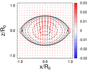
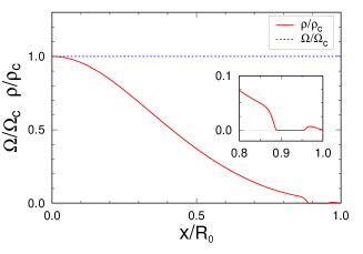
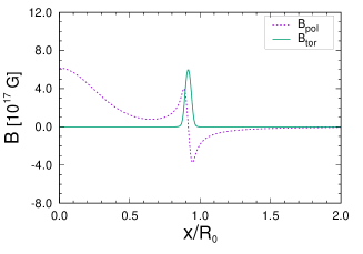
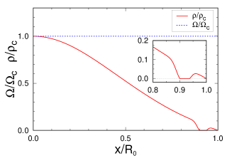
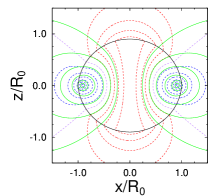
Figure 1: Solutions for uniformly rotating extremely magnetized compact stars associated with an electromagnetic vacuum outside and magnetotunnel (EV-MT-UR type). The panels in the first row correspond to the rapidly rotating model EV-MT-UR-1. The left panel: contours of $p/\rho$ (black closed curves), the poloidal magnetic field (orange arrows), color density map for the toroidal magnetic fields (red and blue), and the boundary of the magnetotunnel (green circles) are shown. The contours of $p/\rho$ are drawn at $p/\rho=0.001,0.002,0.005,0.01,0.02,0.05,0.1$. The middle panel: the rest mass density $\rho/\rho_{c}$ (red curve) and the angular velocity $\Omega/\Omega_{c}$ are plotted along the equatorial radius ($x$-axis). An inset is a close-up of $\rho/\rho_{c}$ near the surface. The right panel: components of the magnetic fields, $B_{\rm pol}=F_{xy}$ (dashed purple curve) and $B_{\rm tor}=-F_{xz}$ (dark green curve) are plotted along the equatorial radius ($x$-axis). The panels in the second row are the same as the first row but for the slowly rotating model EV-MT-UR-2. In the third row, the first panel from the left, the metric potentials are shown, which are the contours of $\psi$ (green closed curves), the color density map for $\tilde{\beta}_{y}$ (red and blue), the contours of $h_{xz}$ (red and blue curves), and the surface of the star (black closed curve). In the second panel from the left, the components of electromagnetic 1-form are shown, which are the contours of $A_{\phi}$ (green curves), the contours of $A_{t}$ (dashed red (positive), purple (zero), blue (negative)), and the surface of the star (black closed curve) for the model EV-MT-UR-1. The third and fourth panels of the third row are the same as the first and the second panels, respectively, but for the model EV-MT-UR-2.

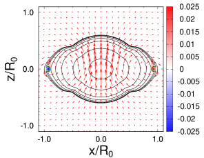
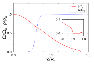
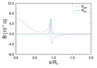
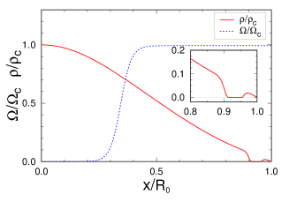
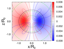
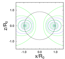
Figure 2: Same as Fig.1 but for differentially rotating and extremely magnetized compact stars associated with a magnetosphere and a magnetotunnel, MS-MT-DR-1 (rapidly rotating model) and MS-MT-DR-2 (slowly rotating model).

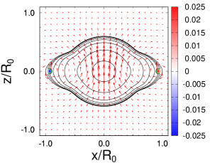
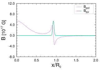
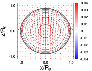
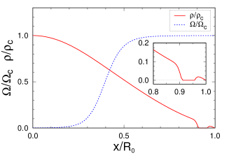
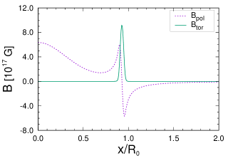
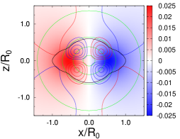
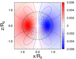
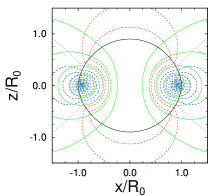
Figure 3: Same as Fig.1 but for differentially rotating and extremely magnetized compact stars associated with an electromagnetic vacuum outside and a magnetotunnel, EV-MT-DR-1 (rapidly rotating model) and EV-MT-DR-2 (slowly rotating model).

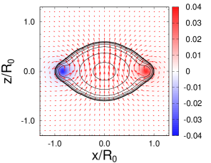
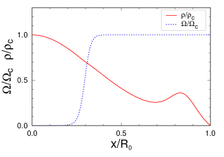
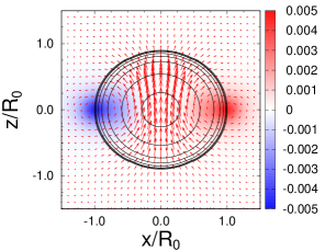
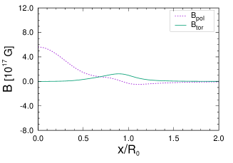
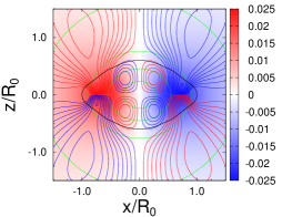
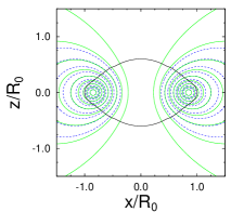
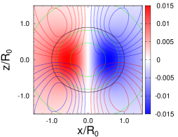
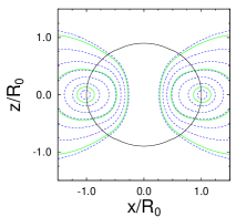
Figure 4: Same as Fig.1 but for differentially rotating and extremely magnetized compact stars associated with a magnetosphere, MS-DR-1 (supramassive model) and MS-DR-2 (normal mass model), whose toroidal magnetic fields are distributed across the stellar support and magnetosphere.

Table 4: Physical quantities of solutions presented in Figs. 1–3. All solutions are calculated with fixing the ratio of the maximum values of the pressure to the rest mass density $(p/\rho)_{\rm c}=0.12322$, which corresponds to the rest mass density $\rho_{\rm c}=1.0717\times 10^{15}\ [\mbox{g/cm}^{3}]$. Listed quantities are the ratio of the equatorial to polar radii in the coordinate length $R_{z}/R_{0}$, the equatorial and polar radii in proper length $\bar{R}_{0}$ and $\bar{R}_{z}$, the angular velocity $\Omega_{\rm c}$ (see, Sec. II.3.3), the ADM mass $M_{\rm ADM}$, the rest mass $M_{0}$, the angular momentum $J$, and a residual of the equality of the Komar mass $M_{\rm K}$ and the ADM mass $M_{\rm ADM}$. Units of listed quantities are explained in Table 3. To convert a unit of length from $G=c=M_{\odot}=1$ to [km], multiply $GM_{\odot}/c^{2}=1.477$[km]. Details of the definitions for these quantities are found in Appendix F of Paper I.

Model	$R_{z}/R_{0}$	$\bar{R}_{0}$	$\bar{R}_{z}/\bar{R}_{0}$	$\Omega_{\rm c}$	$M_{\rm ADM}$	$M_{0}$	$J/M_{\rm ADM}^{2}$	$|1-M_{\rm K}/M_{\rm ADM}|$
EV-MT-UR-1	0.6	12.496	0.62293	$2.9503\times 10^{-2}$	1.4262	1.5356	0.61783	$4.3864\times 10^{-5}$
EV-MT-UR-2	0.9	9.5086	0.90536	$9.6580\times 10^{-3}$	1.2097	1.2986	0.17625	$1.0482\times 10^{-6}$
MS-MT-DR-1	0.6	12.601	0.62341	$2.8048\times 10^{-2}$	1.4323	1.5460	0.51691	$3.9883\times 10^{-3}$
MS-MT-DR-2	0.9	9.5293	0.90550	$8.4512\times 10^{-3}$	1.2066	1.2954	0.12268	$2.7386\times 10^{-4}$
EV-MT-DR-1	0.6	12.972	0.62549	$2.6918\times 10^{-2}$	1.3874	1.4978	0.42490	$5.8742\times 10^{-3}$
EV-MT-DR-2	0.9	9.5423	0.90571	$8.2012\times 10^{-3}$	1.2054	1.2940	0.10204	$3.4697\times 10^{-4}$
MS-DR-1	0.6	12.301	0.62111	$1.6336\times 10^{-2}$	1.5327	1.6301	0.36932	$1.1060\times 10^{-3}$
MS-DR-2	0.9	9.4817	0.90481	$1.4901\times 10^{-2}$	1.2189	1.3100	0.26448	$1.0416\times 10^{-4}$

Table 5: Continued from Table 4, listed quantities are the maximum values of poloidal and toroidal magnetic fields, ${B^{\rm max}_{\rm pol}}$ and ${B^{\rm max}_{\rm tor}}$, the ratios of poloidal and toroidal magnetic field energies, ${\cal M}_{\rm pol}$ and ${\cal M}_{\rm tor}$, and electric field energy, ${\cal M}_{\rm ele}$, to the total electromagnetic field energy ${\cal M}$, the ratios of the kinetic, internal, and electromagnetic field energies to the gravitational energy, ${\cal T}/|{\cal W}|$, $\Pi/|{\cal W}|$, and ${\cal M}/|{\cal W}|$, respectively, and the virial constant $I_{\rm vir}$, and the electric charge contribution from the volume integral of the star $Q_{M}$. Details of the definitions are found in Appendix F in Paper I. The maximums of magnetic field components ${B^{\rm max}_{\rm pol}}$ and ${B^{\rm max}_{\rm tor}}$ are defined by those of spatial Faraday tensor $F_{ab}$ in Cartesian coordinates, ${B_{\rm pol}}:=F_{xy}$ and ${B_{\rm tor}}:=-F_{xz}$.

${B^{\rm max}_{\rm pol}}$[G]	${B^{\rm max}_{\rm tor}}$[G]	${\cal M}_{\rm pol}/{\cal M}$	${\cal M}_{\rm tor}/{\cal M}$	${\cal M}_{\rm ele}/{\cal M}$	${\cal T}/|{\cal W}|$	$\Pi/|{\cal W}|$	${\cal M}/|{\cal W}|$	$I_{\rm vir}/|{\cal W}|$	$Q_{M}$
$6.1604\times 10^{17}$	$5.9686\times 10^{17}$	0.92731	0.036274	0.036413	0.061677	0.28602	0.019016	$4.2789\times 10^{-4}$	$5.5363\times 10^{-2}$
$6.3763\times 10^{17}$	$8.4596\times 10^{17}$	0.95783	0.039465	0.0027073	0.0052941	0.32319	0.020126	$2.9462\times 10^{-4}$	$9.2879\times 10^{-3}$
$6.0341\times 10^{17}$	$5.8367\times 10^{17}$	0.93139	0.031169	0.037446	0.052395	0.28570	0.019147	$1.8954\times 10^{-2}$	$5.3731\times 10^{-2}$
$6.3494\times 10^{17}$	$8.6731\times 10^{17}$	0.96193	0.035946	0.0021234	0.0033736	0.32376	0.020848	$1.1172\times 10^{-3}$	$7.9114\times 10^{-3}$
$5.4290\times 10^{17}$	$5.3893\times 10^{17}$	0.93710	0.035454	0.027449	0.038567	0.29213	0.017490	$2.8983\times 10^{-2}$	$5.0486\times 10^{-2}$
$6.3568\times 10^{17}$	$9.1621\times 10^{17}$	0.96044	0.037997	0.0015662	0.0025140	0.32399	0.021508	$1.4947\times 10^{-3}$	$7.5440\times 10^{-3}$
$1.1258\times 10^{18}$	$7.8558\times 10^{17}$	0.91411	0.070139	0.015746	0.019785	0.26756	0.15293	$4.8131\times 10^{-3}$	$8.9732\times 10^{-2}$
$5.3348\times 10^{17}$	$9.8917\times 10^{16}$	0.92365	0.070049	0.0062992	0.012604	0.32182	0.0090924	$2.4980\times 10^{-4}$	$2.7732\times 10^{-3}$

III Results

From the formulation and numerical method described in Sec. II, compact star solutions associated with extremely strong electromagnetic fields are obtained. Overall configurations of the magnetic fields generated from this formulation are typically the strong poloidal (dipole like) magnetic fields extending from the core of the star to the outside, and the poloidal and toroidal magnetic fields concentrated in a toroidal region near the equatorial surface. In Paper I, we have observed that the latter very strong mixed magnetic fields expel the matter near the equatorial surface. As mentioned above, we introduce the force-free magnetic fields when the matter is totally expelled that the mass density becomes negligible in the toroidal region, so the force free magnetotunnel is formed inside of the compact star.

Combining the electromagnetic vacuum or magnetosphere, and the uniform or differential rotations, we present four types of such extremely magnetized solutions in this article where three of them are associated with the magnetotunnel:

• EV-MT-UR type – those associated with the electromagnetic vacuum outside of the star, magnetotunnel, and uniform rotation.

• MS-MT-DR type – those associated with the magnetosphere, magnetotunnel, and differential rotation.

• EV-MT-DR type – those associated with the electromagnetic vacuum outside, magnetotunnel, and differential rotation.

• MS-DR type – those associated with the magnetosphere, and differential rotation whose toroidal magnetic field is distributed across the star and the magnetosphere.

III.1 Overall feature of solutions with magnetotunnel

III.1.1 Uniformly rotating models with electromagnetic vacuum outside

In Fig. 1, EV-MT-UR models with rapid and slow rotations are shown. These are straightforward extensions of solutions presented in Paper I, in particular changing the parameters $\{\Lambda_{0},\Lambda_{\phi 0}\}$ of the model P1 systematically to achieve stronger electromagnetic fields. The boundaries of the force-free magnetotunnel, where the toroidal regions where the matter is totally expelled by the magnetic fields, are indicated with green circles in the left panel of the first and the second rows for rapidly and slowly rotating models, respectively. The expelled regions can be also seen clearly in the rest mass density profile $\rho/\rho_{c}$ (red curves) along the equatorial radius $x/R_{0}$ plotted in the middle panels of the first and the second row.

The right panel of the first and the second rows in Fig. 1 are the plots of the poloidal, $B_{\rm pol}=F_{xy}$, and the toroidal, $B_{\rm tor}=-F_{xz}$, components of magnetic fields along the equatorial radius $x/R_{0}$. The maximum of $B_{\rm pol}$ is at the center of the star, while that of $B_{\rm tor}$ is near the equatorial surface. It can be seen that the poloidal component $B_{\rm pol}$ takes a large value also around this toroidal region near the equatorial surface. It is also noticeable that, for the slowly rotating EV-MT-UR-2 model, the maximum value of $B_{\rm tor}$ is greater than that of $B_{\rm pol}$.

In the second and fourth panels in the third row, the contours of the components of electromagnetic 1-form $A_{t}$ and $A_{\phi}$ are drawn. Because $A_{t}$ is assumed to be a function of $A_{\phi}$ in the ideal MHD region of the stellar support satisfying the relation (38), their contours are homologous there, while they are not in the electromagnetic vacuum outside of the star.

III.1.2 Differentially rotating models with magnetosphere

In Fig. 2, MS-MT-DR models with rapid and slow rotations are shown. The same as the EV-MT-UR model in Fig. 1, the strong concentration of the magnetic fields expels the matter near the equatorial surface and form the magnetotunnel, which can be seen in the corresponding panels in Fig. 2.

Differences between MS-MT-DR model and the previous EV-MT-UR model are the magnetosphere outside of the star instead of electromagnetic vacuum, and the differential rotation instead of the uniform rotation. As discussed in Sec. II, arbitrary functions in the force-free magnetosphere/magnetotunnel region are chosen to be the same as those in ideal MHD region as Eq. (24) that the electromagnetic potentials are smoothly connected across the boundaries of these regions. This can be seen in the second and the fourth panels of the third row in Fig. 2 for the contours of $A_{t}$ and $A_{\phi}$, which are homologous not only on the stellar support (ideal MHD region) but also in the force-free region outside of the star (as well as in the magnetotunnel region).

We also introduce the differential rotation as prescribed in Eq. (40) in this model. As shown in the middle panels of the first and the second row of Fig. 2, the profiles of $\Omega/\Omega_{c}$ are increasing along the equatorial radius $x/R_{0}$. These are rather uncommon profiles for differential rotation laws, that is, in most of numerical computations of relativistic rotating stars, differential rotation laws with decreasing $\Omega$ along $x/R_{0}$ have been considered RNSdiff , except for a few works RNSdiff2 . There are two motivations for us to choose this new differential rotation law (40).

In computing solutions with force-free magnetosphere outside, we found that the $t$-component of electromagnetic 1-form $A_{t}$ diverges asymptotically if we assume uniform rotation. This may be understood that in our assumptions, namely the stationary and axisymmetric force-free magnetosphere, the magnetic field lines attached to the stellar surface have to rotate with the same $\Omega$ even if they are extended to the region outside of the light cylinder. In terms of our formulation, it appears that the current $j^{t}$ coupled with the $\phi$-component $j^{\phi}$ as in Eq. (18) doesn’t fall-off asymptotically fast enough to have a regular asymptotic behavior in $A_{t}$. Since the magnetic field lines extended towards the region of larger $r$ are attached to the surface of the star closer to the axis of rotation ($z$-axis), setting $A_{t}^{\prime}=\Omega(A_{\phi})$ to vanish near the rotation axis decouples the $j^{\phi}$ and $j^{t}$ in the large $r$ region. This is the first reason that we choose the differential rotation law (40), which is non-rotating near the axis of symmetry. Also for this reason, it seems it is not possible to obtain uniformly rotating relativistic solutions with the force-free magnetosphere using our formulation. In the literature, only the non-rotating solutions are calculated for such strongly magnetized relativistic stars associated with the force-free magnetosphere in general relativity Pili:2014zna . The second reason for this differential rotation law is motivated by the results of simulations Tsokaros:2021pkh and a semi analytic argument Shapiro:2000zh that such rotation profiles may, although transiently, appear during the evolution of highly magnetized rotating stars.

Because of the differential rotation, the rotation period of the field lines in the magnetosphere differs with latitude. The fastest ones are those attached near the equatorial surface. The smallest cylindrical radius of the light cylinder becomes around $\varpi=r\sin\theta\sim 2\pi/\Omega_{c}\sim 24R_{0}$ $(100R_{0})$ for the rapidly (slowly) rotating model MS-MT-DR-1 (2, respectively), so the rotating field lines do not reach to the light cylinder in our models.

III.1.3 Differentially rotating models with electromagnetic vacuum outside

In Fig. 3, EV-MT-DR models with rapid and slow rotations are shown. This is to demonstrate that it is possible to calculate solutions combining the electromagnetic vacuum region outside and the differential rotation. Because of the magnetic vacuum, the field lines outside are not dragged around. Although in principle, one can freely specify the differential rotation law for these models, we only modify the values of parameters slightly from MS-MT-DR models. It appears that interior magnetic fields of EV-MT-DR models are similar to those of MS-MT-DR models rather than EV-MT-UR models.

III.2 Solutions with toroidal fields distributed across the star and the magnetosphere

Because of our previous choices of parameter, in particular $A_{\phi}^{0}$ for the function (33) (see Table 2), the function varies when the potential $A_{\phi}$ becomes larger than its value at the equatorial surface, $A_{\phi}>A_{\phi}^{0}=A_{\phi,\rm S}^{\rm max}$. Because of this, the toroidal component of the magnetic field is confined interior of the compact star. This choice was necessary for the EV models since the toroidal magnetic field can not exist in the vacuum region. Also because of this, the extremely strong magnetic fields develop near the equatorial surface, which is strong enough to expel the matter as shown in Sec. III.1.

For the MS models, however, the toroidal component of the magnetic fields is allowed to exist in the region of force-free magnetosphere outside of the star. In Fig. 4, we successfully computed such strongly magnetized solutions whose toroidal component of magnetic fields is distributed across the star and the magnetosphere. For these solutions with the magnetosphere, the parameter $A_{\phi}^{0}$ is chosen to be $A_{\phi}^{0}=0.3A_{\phi,\rm S}^{\rm max}$, and $A_{\phi}^{1}$ is also modified as $A_{\phi}^{1}=1.7A_{\phi}^{\rm max}$ (see, Table 2).

As seen in Fig. 4, the peak of toroidal component near the equatorial surface becomes broader and less concentrated compared with the other magnetotunnel models in previous Sec.III.1. For these MS-DR models, we couldn’t find a solution with magnetotunnel in a parameter region we searched solutions. As shown in Fig. 4, for the largely deformed model MS-DR-1, the matter is expelled in a wider region, but not totally. For the less deformed model MS-DR-2, on the other hand, we couldn’t compute a solution with the same parameter, but obtained a solution with smaller and broader peak of the toroidal component. The maximum of the toroidal component of this model is close to the stellar surface.

III.3 Physical quantities of solutions

In Tables 4 and 5, physical quantities of solutions presented in Figs. 1-4 are listed. For all models (for both of rapidly and slowly rotating cases), we choose the same central (maximum) rest mass density $\rho_{c}$. As shown in the tables, for the solutions with the magnetotunnel, the rest mass $M_{0}$ are around $1.5M_{\odot}$ and $1.3M_{\odot}$ for the rapidly and slowly rotating models, respectively. Hence, in our unit (choice of the polytropic constant $K$), corresponding non-rotating and non-magnetized solutions, that is spherically symmetric TOV solutions, with the same rest mass have the compactness around $M/R\sim 0.2$ and $M/R\sim 0.15$, respectively. Therefore, these solutions are mildly compact models. On the other hand, the MS-DR-1 is a supramassive model associated with the strongest electromagnetic fields among other models.

From the virial relation with an equality $M_{\rm ADM}=M_{\rm K}$ virial ,

$$I_{\rm vir}\,:=\,2{\cal T}+3\Pi+{\cal M}+{\cal W}=0,$$ (43)

one can roughly understand the contribution of the kinetic term ${\cal T}$ and electromagnetic term ${\cal M}$ to the deformation of the compact stars. For the solutions with the magnetotunnel, $2{\cal T}$ are around 4-6 times of ${\cal M}$ for the rapidly rotating models, while for the slowly rotating models ${\cal M}$ is dominating about 2-3.5 times over $2{\cal T}$. The ratios of $(2{\cal T}+{\cal M})/3\Pi$ which roughly measure contribution of non-spherical deformation to the equilibriums are about 3% for the slowly rotating models, and 15% for the rapidly rotating models. For the MS-DR-1 model, on the other hand, ${\cal M}$ is dominating over $2{\cal T}$, where ${\cal M}$ is about 4 times larger than $2{\cal T}$. The value of ${\cal M}/|\cal W|$ is about 7 times larger than the other models.

It is also commented that, for the models with the magnetotunnel, the maximum values of the toroidal components of magnetic fields are comparable or even larger than that of poloidal magnetic fields, overall integrals of toroidal fields ${\cal M}_{\rm tor}$ are only 3.5-4% of those of poloidal fields ${\cal M}_{\rm pol}$. The integrals of electric part ${\cal M}_{\rm ele}$ is about the same as ${\cal M}_{\rm tor}$ for the rapidly rotating models, but it is less than 10% of ${\cal M}_{\rm tor}$ for the slowly rotating models. This seems to be reasonable considering that the higher multipole contributions are less dominating in the slowly rotating models. For the MS-DR models, the toroidal component of magnetic field is distributed in broader region, and hence the fraction of ${\cal M}_{\rm tor}/{\cal M}$ is about twice of the other models, although it is still more than an order smaller than the contribution from the poloidal component ${\cal M}_{\rm pol}/{\cal M}$.

IV Discussion

Results of simulations by Braithwaite and co-workers Braithwaite suggest that stable equilibriums of strongly magnetized stars may be achieved when the energies of the poloidal and the toroidal components of magnetic fields become comparable Braithwaite . One of motivations to investigate the solutions of such mixed poloidal and toroidal magnetic fields presented in this paper is to obtain such stable models of magnetized compact stars. However, so far, the energy carried by the toroidal field is far smaller than that of the poloidal field in our models. Recently we have performed numerical simulations of such extremely magnetized compact stars starting from the initial data calculated in Paper I (and with varied parameters) which are close to the EV-MT-UR models but with ${B^{\rm max}_{\rm tor}}$ around 30-40% smaller Tsokaros:2021pkh . We found the kink instability develop and destroy the axisymmetry of the solutions, although in a certain case the instability develop slower than the alfvén time. Also found was the magnetorotational effect carries away the angular momentum of the stellar core, hence the rotation of the core slows down and a differential rotation develops. It is totally unclear, but is interesting to investigate, how the stronger toroidal magnetic field, and/or a differential rotation as in the present models modify the evolutions of such compact stars.

The Magnetic field strength of the solutions presented in this paper may be too strong for astrophysically realistic compact objects. From a theoretical stand point, however, it is of interest to investigate the extreme cases where the electromagnetic fields affect the stellar equilibrium or even become a source of gravity. In the above solutions, it is observed that the magnetic fields locally dominate over the hydrostatic equilibriums, but the metric is affected only slightly. As seen in the contours of metric components in Figs. 1-4, in the toroidal region near the equatorial surface where the strong magnetic fields are concentrated, the contour for $\psi$ and the density map of $\tilde{\beta}_{y}$ appears to be unaffected, while some structure is observed in the contours of $h_{xz}$ in this region. Hence, the limit of the strength of magnetic field is not reached in a sense that it is not a dominant source of gravity. Since our numerical method solves the full set of Einstein’s and Maxwell’s equations for equilibrium or quasi-equilibrium initial data, we expect that even more extreme magnetic fields may be obtained, including an extremely strong magnetosphere surrounding a black hole. Such studies may be one of future extensions of the present work.

- (1) R. C. Duncan and C. Thompson, Astrophys. J. 392, L9 (1992); B. Paczynski, Acta Astron. 42, 145-153 (1992)
- (2) For reviews, see e.g., V. M. Kaspi and A. Beloborodov, Ann. Rev. Astron. Astrophys. 55, 261 (2017); R. Turolla, S. Zane and A. Watts, Rept. Prog. Phys. 78, no. 11, 116901 (2015); P. Esposito, N. Rea and G. L. Israel, Astrophys. Space Sci. Libr. 461, 97-142 (2020)
- (3) K. Konno, T. Obata and Y. Kojima, Astron. Astrophys. 352, 211 (1999). K. Ioka and M. Sasaki, Phys. Rev. D 67, 124026 (2003); K. Ioka and M. Sasaki, Astrophys. J. 600, 296 (2004); R. Ciolfi, V. Ferrari, L. Gualtieri and J. A. Pons, Mon. Not. Roy. Astron. Soc. 397, 913 (2009); R. Ciolfi, V. Ferrari and L. Gualtieri, Mon. Not. Roy. Astron. Soc. 406, 2540 (2010); S. Yoshida, K. Kiuchi and M. Shibata, Phys. Rev. D 86, 044012 (2012); S. Yoshida, Phys. Rev. D 99, no.8, 084034 (2019)
- (4) A. Tsokaros and K. Uryū, [arXiv:2112.05162 [gr-qc]].
- (5) K. Kiuchi, K. Kyutoku, Y. Sekiguchi and M. Shibata, Phys. Rev. D 97, no. 12, 124039 (2018); R. Ciolfi, W. Kastaun, J. V. Kalinani and B. Giacomazzo, Phys. Rev. D 100, no. 2, 023005 (2019); M. Ruiz, A. Tsokaros, V. Paschalidis and S. L. Shapiro, Phys. Rev. D 99, no. 8, 084032 (2019) K. Kiuchi, K. Kyutoku and M. Shibata, Phys. Rev. D 86, 064008 (2012); P. Mösta et al., Astrophys. J. 785, L29 (2014); P. Mösta, C. D. Ott, D. Radice, L. F. Roberts, E. Schnetter and R. Haas, Nature 528, 376 (2015)
- (6) A. Tsokaros, M. Ruiz, S. L. Shapiro and K. Uryū, Phys. Rev. Lett. 128, no.6, 061101 (2022)
- (7) K. Uryu, E. Gourgoulhon, C. Markakis, K. Fujisawa, A. Tsokaros and Y. Eriguchi, Phys. Rev. D 90, no. 10, 101501(R) (2014)
- (8) K. Uryu, S. Yoshida, E. Gourgoulhon, C. Markakis, K. Fujisawa, A. Tsokaros, K. Taniguchi and Y. Eriguchi, Phys. Rev. D 100, no.12, 123019 (2019)
- (9) X. Huang, C. Markakis, N. Sugiyama and K. Uryu, Phys. Rev. D 78, 124023 (2008); K. Uryu and A. Tsokaros, Phys. Rev. D 85, 064014 (2012); K. Uryu, A. Tsokaros and P. Grandclement, Phys. Rev. D 86, 104001 (2012); A. Tsokaros, K. Uryu and L. Rezzolla, Phys. Rev. D 91, no. 10, 104030 (2015)
- (10) M. Bocquet, S. Bonazzola, E. Gourgoulhon and J. Novak, Astron. Astrophys. 301, 757 (1995)
- (11) K. Glampedakis, S. K. Lander and N. Andersson, Mon. Not. Roy. Astron. Soc. 437, no. 1, 2 (2014);
- (12) A. G. Pili, N. Bucciantini and L. Del Zanna, Mon. Not. Roy. Astron. Soc. 447, 2821 (2015)
- (13) K. Kiuchi and S. Yoshida, Phys. Rev. D 78, 044045 (2008) J. Frieben and L. Rezzolla, Mon. Not. Roy. Astron. Soc. 427, 3406 (2012) A. G. Pili, N. Bucciantini and L. Del Zanna, Mon. Not. Roy. Astron. Soc., 439, 3541 (2014); A. G. Pili, N. Bucciantini and L. Del Zanna, Mon. Not. Roy. Astron. Soc. 470, no. 2, 2469 (2017)
- (14) H. Komatsu, Y. Eriguchi, and I. Hachisu, Mon. Not. Roy. Astron. Soc. 239, 153 (1989); M. Ansorg, D. Gondek-Rosinska, L. Villain and M. Bejger, EAS Publ. Ser. 30, 373 (2008); D. Gondek-Rosinska, I. Kowalska, L. Villain, M. Ansorg and M. Kucaba, Astrophys. J. 837, no. 1, 58 (2017); A. M. Studzinska, M. Kucaba, D. Gondek-Rosinska, L. Villain and M. Ansorg, Mon. Not. Roy. Astron. Soc. 463, no. 3, 2667 (2016); T. W. Baumgarte, S. L. Shapiro and M. Shibata, Astrophys. J. 528, L29 (2000); I. A. Morrison, T. W. Baumgarte and S. L. Shapiro, Astrophys. J. 610, 941 (2004); J. D. Kaplan, C. D. Ott, E. P. O’Connor, K. Kiuchi, L. Roberts and M. Duez, Astrophys. J. 790, 19 (2014); F. Galeazzi, S. Yoshida and Y. Eriguchi, Astron. Astrophys. 541, A156 (2012); A. Bauswein and N. Stergioulas, Mon. Not. Roy. Astron. Soc. 471, 4956 (2017); G. Bozzola, N. Stergioulas and A. Bauswein, Mon. Not. Roy. Astron. Soc. 474, no.3, 3557-3564 (2018); K. Uryu, A. Tsokaros, F. Galeazzi, H. Hotta, M. Sugimura, K. Taniguchi and S. Yoshida, Phys. Rev. D 93, no. 4, 044056 (2016); E. Zhou, A. Tsokaros, K. Uryu, R. Xu and M. Shibata, Phys. Rev. D 100, no.4, 043015 (2019); M. Szkudlarek, D. Gondek-Rosińska, L. Villain and M. Ansorg, Astrophys. J. 879, no.1, 44 (2019); A. Tsokaros, M. Ruiz, L. Sun, S. L. Shapiro and K. Uryū, Phys. Rev. Lett. 123, no.23, 231103 (2019).
- (15) K. Uryu, A. Tsokaros, L. Baiotti, F. Galeazzi, K. Taniguchi and S. Yoshida, Phys. Rev. D 96, no.10, 103011 (2017); A. Passamonti and N. Andersson, Mon. Not. Roy. Astron. Soc. 498, no.4, 5904-5915 (2020); X. Xie, I. Hawke, A. Passamonti and N. Andersson, Phys. Rev. D 102, no.4, 044040 (2020); P. Iosif and N. Stergioulas, Mon. Not. Roy. Astron. Soc. 503, no.1, 850-866 (2021); G. Camelio, T. Dietrich, S. Rosswog and B. Haskell, Phys. Rev. D 103, no.6, 063014 (2021); P. Iosif and N. Stergioulas, Mon. Not. Roy. Astron. Soc. 510, no.2, 2948-2967 (2022); K. Franceschetti, L. Del Zanna, J. Soldateschi and N. Bucciantini, Universe 8, no.3, 172 (2022).
- (16) S. L. Shapiro, Astrophys. J. 544, 397-408 (2000)
- (17) E. Gourgoulhon, and S. Bonazzola, Classical and Quantum Gravity, 11, 443 (1994); R. Beig, Physics Letters A, 69, 153 (1978); M. Shibata, K. Uryu and J. L. Friedman, Phys. Rev. D 70, 044044 (2004) [Erratum-ibid. D 70, 129901 (2004)]
- (18) J. Braithwaite and H. C. Spruit, Nature 431, 819 (2004); J. Braithwaite and H. C. Spruit, Astron. Astrophys. 450, 1097 (2006); J. Braithwaite and A. Nordlund, Astron. Astrophys. 450, 1077 (2006); [arXiv:astro-ph/0510316 [astro-ph]]. J. Braithwaite, Mon. Not. Roy. Astron. Soc. 397, 763 (2009)