Lancester correlation - a new dependence measure linked to maximum correlation

Abstract

We suggest correlation coefficients together with rank - and moment based estimators which are simple to compute, have tractable asymptotic distributions, equal the maximum correlation for a class of bivariate Lancester distributions and in particular for the bivariate normal equal the absolute value of the Pearson correlation, while being only slightly smaller than maximum correlation for a variety of bivariate distributions. In a simulation the power of asymptotic as well as permutation tests for independence based on our correlation measures compares favorably to various competitors, including distance correlation and rank coefficients for functional dependence. Confidence intervals based on the asymptotic distributions and the covariance bootstrap show good finite-sample coverage.

Keywords: Correlation coefficient; Independence tests; Lancester distribution; Rank statistics.

1 Introduction

Measuring the correlation between random quantities is a basic task for statisticians. The most commonly used correlation coefficients for real-valued observations are Pearson’s correlation coefficient as well as Spearman’s $\rho$ and Kendell’s $\tau$, designed for detecting linear and monotone relationships, respectively. Still, additional requirements such as characterizing independence (Székely et al., 2007), regression dependence (Dette et al., 2013; Wang et al., 2017; Chatterjee, 2021), or consistency axioms (Bergsma and Dassios, 2014; Weihs et al., 2018), among others, led to a variety of novel correlation coefficients.

In terms of axiomatic properties, the benchmark may be considered to be the maximum correlation introduced by Hirschfeld (1935) and Gebelein (1941). It is defined for non-constant random variables $X,Y$ on the same probability space with values in potentially abstract measurable spaces $\mathcal{X}$, $\mathcal{Y}$ by

$$\rho_{\text{max}}(X,Y)=\sup_{\phi,\psi}\,\mathbb{E}\big{[}\phi(X)\,\psi(Y)\big{]},$$ (1)

where the supremum is taken over

$$\phi:\mathcal{X}\to\mathbb{R},\ \mathbb{E}[\phi(X)]=0,\ \mathbb{E}[\phi^{2}(X)]=1,\quad$$ (2)

and similarly for $\psi$ and $Y$. Rényi (1959) sets up a list of axiomatic properties for correlation coefficients, including symmetry, characterization of independence and functional dependence, and invariance under monotone transformations, and shows that these are satisfied by maximum correlation. Further, for the normal distribution it equals the absolute value of Pearson’s correlation coefficient (Gebelein, 1941), see also Lancaster (1957).

While maximum correlation is still of broad theoretical and applied interest (Lopez-Paz et al., 2013; Anantharam et al., 2013; Huang and Zhu, 2016; Baharlouei et al., 2019), there are some downsides with its involved definition as a supremum in (1). First, it is hard to estimate, and while the ACE algorithm of Breiman and Friedman (1985) is a well - established tool to do so, it gives only raw estimates so that tests for independence or confidence intervals are not readily available. Furthermore maximum correlation is sometimes considered to be close to or even equal to $1$ for too many joint distributions (Pregibon and Vardi, 1985; Chatterjee, 2021).

Suppose that $X$ and $Y$ are marginally standard normally distributed with joint density $f_{X,Y}$. Sarmanov and Bratoeva (1967) characterize the densities $f_{X,Y}$ which are of finite squared contingency in the sense of Pearson (1904) and admit diagonal expansions in terms of Hermite polynomials, see also Lancaster (1958, 1963). Their results imply that the maximum correlation is then given as

$$\rho_{\text{max}}(X,Y)=\max\big{(}|\rho_{\text{Pear}}(X,Y)|,\rho_{\text{Pear}}(X^{2},Y^{2})\big{)},$$ (3)

where $\rho_{\text{Pear}}$ is the Pearson correlation coefficient. For the bivariate normal, this reduces to $|\rho_{\text{Pear}}(X,Y)|$. The expansions in terms of canonical forms on which (3) is based give rise to the class of so-called Lancester distributions, for recent results beyond normal margins see Buja (1990); Koudou (1998); Papadatos and Xifara (2013).

The representation (3) is the formal motivation for introducing our correlation coefficient, which we shall call the Lancester correlation coefficient. We set

$$\rho_{\text{L}}(X,Y)=\max\big{(}|\rho_{\text{Pear}}(\tilde{X},\tilde{Y})|,\big{|}\rho_{\text{Pear}}(\tilde{X}^{2},\tilde{Y}^{2})\big{|}\big{)},\quad\tilde{X}=\Phi^{-1}(F_{X}(X)),$$ (4)

$\tilde{Y}$ is defined analogously to $\tilde{X}$, and $\Phi$ denotes the distribution function of the standard normal and $F_{X}$ and $F_{Y}$ are the distribution functions of $X$ and $Y$, respectively. If $X$ and $Y$ have continuous marginal distributions such that the distribution of $(\tilde{X},\tilde{Y})$ falls into the class discussed in Sarmanov and Bratoeva (1967), then actually $\rho_{\text{L}}(X,Y)=\rho_{\text{max}}(X,Y)$, otherwise, $\rho_{\text{L}}(X,Y)$ is a lower bound for $\rho_{\text{max}}(X,Y)$. For general distributions, $\rho_{\text{L}}(X,Y)$ measures the linear correlation between $\tilde{X}$ and $\tilde{Y}$ as well as between their squares. As we shall illustrate numerically this suffices to capture most of $\rho_{\text{max}}(X,Y)$ for a variety of distributions. Also note that $\rho_{\text{Pear}}(\tilde{X},\tilde{Y})$ is closely related to the Spearman correlation coefficient, with scores from the normal quantile function in the spirit of the van der Waerden test (Van der Waerden, 1952). Such transformations are known under various names, e.g. rank-based inverse normal in psychology (Beasley et al., 2009; Bishara and Hittner, 2017). We propose a rank-based estimator for $\rho_{\text{L}}(X,Y)$, together with a second correlation coefficient with a simple moment standardization and an empirical moment-based estimator. Both have tractable asymptotic distributions, and numerical experiments show good coverage properties of confidence intervals based on asymptotics and the covariance bootstrap. The power of asymptotic as well as permutation tests for independence based on our correlation measures compares favorably in simulations to various competitors, including distance correlation (Székely et al., 2007), the rank coefficient for functional dependence by Chatterjee (2021) or the $\tau^{*}$ - coefficient of Bergsma and Dassios (2014).

2 Maximum correlation and the Lancester correlation coefficient

In this section we further motivate and illustrate our novel correlation coefficient $\rho_{\text{L}}(X,Y)$ in (4). We start by recalling the nonparametric class of densities for which (3), our point of departure, holds true. Let $\varphi(x)$ denote the density of the standard normal distribution, and suppose that $X$ and $Y$ have standard normal margins. The density $f_{X,Y}$ of $(X,Y)$ is by definition of finite squared contingency if and only if $f_{X,Y}(x,y)/(\varphi(x)\,\varphi(y))$ is square - integrable in the $L_{2}$-space with the bivariate standard Gaussian measure. Then if the canonical variables, that is the singular functions of the conditional expectation operators, are the Hermite polynomials $H_{k}$, $f_{X,Y}$ has an expansion

$$f_{X,Y}(x,y)=\varphi(x)\,\varphi(y)\,\Big{(}1+\sum_{k=1}c_{k}\,H_{k}(x)\,H_{k}(y)\Big{)},$$ (5)

see Lancaster (1958, Theorem 3). Here, $c_{k}$ is the Pearson correlation coefficient of $H_{k}(X)$ and $H_{k}(Y)$. Conversely, Sarmanov and Bratoeva (1967) show that (5) defines a density if and only if $c_{k}=\mathbb{E}[V^{k}]$ is the moment sequence of some random variable $V$ with support in $(-1,1)$. By expanding the functions $\phi$ and $\psi$ in (2) in the definition of the maximum correlation into Hermite series, one finds that $\rho_{\text{max}}(X,Y)$ equals the supremum over $|c_{k}|$, and from the representation of $c_{k}$ as moments of $V$ this results in $\max(|c_{1}|,c_{2})$, that is, (3).

Before we proceed to numerical illustrations on a variety of distributions, as an alternative to (4) let us also introduce the linear Lancester correlation coefficient as

$$\rho_{\text{L,l}}(X,Y)=\max\big{(}|\rho_{\text{Pear}}(X,Y)|,|\rho_{\text{Pear}}(\breve{X}^{2},\breve{Y}^{2})|\big{)},$$ (6)

where $\breve{X}=(X-\mathbb{E}[X])/\text{sd}(X)$ and $\breve{Y}$ are the standardized versions of $X$ and $Y$ and we assume $\mathbb{E}[X^{4}]<\infty$, $\mathbb{E}[Y^{4}]<\infty$.

To illustrate, we first consider bivariate normal mixtures $pf_{1}(x,y,-1/2)+(1-p)$ $f_{1}(x,y,1/2)$, where $f_{1}(x,y,\rho)$ denotes the density of a bivariate normal distribution with standard normal marginals and correlation coefficient $\rho$. For $p=1/2$, one has $\rho_{\text{Pear}}=0,\,\rho_{\text{max}}=1/4$, called NM1. Distribution NM2 uses $p=1/3$, resulting in $\rho_{\text{Pear}}=1/6,\,\rho_{\text{max}}=1/4$ (Sarmanov and Bratoeva, 1967). Scatterplots of the two distributions based on a sample of size 10000 are shown in the left and middle panel of Fig. 1.

Figure 1: Scatterplot with sample size $n=10000$ of two bivariate normal mixtures (NM1, NM2) and bivariate $t$-distribution with 5 degrees of freedom (BVT5)

Estimates of various dependence measures for these datasets can be found in Table 1. Besides $\widehat{\rho_{\text{Pear}}}$ and $\widehat{\rho_{\text{S}}}$, the empirical versions of Pearson’s and Spearman’s correlation coefficients, we use $\widehat{\rho_{\text{L,l}}}$ and $\widehat{\rho_{\text{L}}}$, defined in Section 3, as estimators of $\rho_{\text{L,l}}$ and $\rho_{\text{L}}$. Further, $\widehat{\rho_{\text{ace}}}$, the estimate of $\rho_{\text{max}}$ computed by the ace algorithm in the R package acepack (Spector et al., 2016); the empirical distance correlation $\widehat{\text{dCor}}$ (Rizzo and Szekely, 2022); the empirical value $t^{*}$ of the $\tau^{*}$ coefficient of Bergsma and Dassios (2014), computed with the R package TauStar (Weihs, 2019); finally, $\widehat{\xi}$, the empirical version of the $\xi$-coefficient of Chatterjee (2021).

Findings: For NM1, the values of $\widehat{\rho_{\text{L,l}}},\widehat{\rho_{\text{L}}}$ and $\widehat{\rho_{\text{ace}}}$ are close to $\rho_{\text{max}}=1/4$, as expected. Whereas $\widehat{\text{dCor}}$ is quite small, $t^{*}$ and $\widehat{\xi}$ do not detect the dependence at all. For NM2, $\widehat{\rho_{\text{Pear}}},\widehat{\rho_{\text{S}}},\widehat{\rho_{\text{ace}}}$ and $\widehat{\text{dCor}}$ estimate the linear dependence 1/6; only $\widehat{\rho_{\text{L,l}}}$ and $\widehat{\rho_{\text{L}}}$ have estimates close to $\rho_{\text{max}}=1/4$. Again, $t^{*}$ and $\widehat{\xi}$ do not detect the dependence.

distribution	$\widehat{\rho_{\text{Pear}}}$	$\widehat{\rho_{\text{S}}}$	$\widehat{\rho_{\text{L,l}}}$	$\widehat{\rho_{\text{L}}}$	$\widehat{\rho_{\text{ace}}}$	$\widehat{\text{dCor}}$	$t^{*}$	$\widehat{\xi}$
NM1	0.002	-0.006	0.279	0.279	0.256	0.062	0.001	0.005
NM2	0.154	0.145	0.237	0.238	0.155	0.147	0.008	0.014
BVT5	-0.010	0.000	0.190	0.210	0.210	0.060	0.000	0.000
BVC	-	0.004	-	0.718	0.992	-	0.006	0.046
Unif-disc	0.002	0.002	0.335	0.267	0.334	0.076	0.002	0.022
GARCH(2,1)	0.021	0.020	0.563	0.516	0.559	0.139	0.002	0.032

Table 1: Estimates of correlation measures for several distributions, each based on one sample with size $n=10000$

The right panel of Fig. 1 shows a scatterplot of the bivariate (standard) $t$-distributions with 5 degrees of freedom and linear correlation $\rho_{\text{Pear}}=0$, called BVT5. A similar plot for the bivariate standard Cauchy distribution (BVC) and a uniform distribution on the unit disc (Unif-disc) is shown in the left and middle panel of Fig. 2. Pearson correlation exists and equals zero for the first and the third distribution; $\rho_{\text{S}}=0$ in all three cases. As is well known, the only independent spherically symmetric distributions are normal distributions. For Unif-disc, it is known that $\rho_{\text{max}}=0.3$ (Buja, 1990).

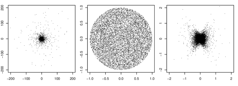
Figure 2: Scatterplot with sample size $n=10000$ of bivariate Cauchy (BVC), uniform distribution on the disc (Unif-disc) and GARCH(2,1)

Findings: Clearly, $\widehat{\rho_{\text{Pear}}}$ and $\widehat{\rho_{\text{S}}}$ can not capture the dependence for neither of the three distributions; the same holds for $t^{*}$ and $\widehat{\xi}$. For BVT5, $\widehat{\rho_{\text{L,l}}},\widehat{\rho_{\text{L}}}$ and $\widehat{\rho_{\text{ace}}}$ give similar values around 0.2; $\widehat{\text{dCor}}$ is rather small. For BVC, $\widehat{\rho_{\text{L}}}$ and $\widehat{\rho_{\text{ace}}}$ take quite large values; $\widehat{\rho_{\text{Pear}}},\widehat{\rho_{\text{L,l}}}$ and $\widehat{\text{dCor}}$ are not defined. For Unif-disc, $\widehat{\rho_{\text{L,l}}},\widehat{\rho_{\text{L}}}$ and $\widehat{\rho_{\text{ace}}}$ take values around 0.3, $\widehat{\text{dCor}}$ is again rather small.

Stock returns $r_{t}$ are typically uncorrelated with their own past $r_{t-1}$ (if stock markets are efficient), but their squares $r_{t}^{2}$ and $r_{t-1}^{2}$ are not. To illustrate the behaviour of our new correlation measures for a typical statistical model for returns, we generate $r_{t}$ using a GARCH(2,1) process with parameters $\alpha=(0.01,0.6)$ and $\beta=0.2$. It is well known that $\rho_{\text{Pear}}=0$ holds for the distribution of the pairs $(r_{t},r_{t-1})$. A scatterplot of $(r_{t},r_{t-1})$ is shown in the right panel of Fig. 2, estimates based on a sample of size 10000 are given in Table 1.

Findings: $\widehat{\rho_{\text{Pear}}}$ and $\widehat{\rho_{\text{S}}}$ are close to zero as expected, but the same holds for $t^{*}$ and $\widehat{\xi}$. While $\widehat{\text{dCor}}$ is around 0.15, $\widehat{\rho_{\text{L,l}}},\widehat{\rho_{\text{L}}}$ and $\widehat{\rho_{\text{ace}}}$ take values larger than 0.5.

3 Estimation and asymptotic inference

Let us discuss estimation of $\rho_{\text{L,l}}(X,Y)$ and of $\rho_{\text{L}}(X,Y)$ based on an i.i.d. sample $(X_{1},Y_{1}),$ $\ldots,$ $(X_{n},Y_{n})$ from the distribution of $(X,Y)$.

First consider $\rho_{\text{L,l}}(X,Y)$, set $\rho_{\text{l1}}=\rho_{\text{Pear}}(X,Y)$ and $\rho_{\text{l2}}=\rho_{\text{Pear}}(\breve{X}^{2},\breve{Y}^{2})$, see (6). Let $\widehat{\rho_{\text{l1}}}$ be the sample correlation, and let $\widehat{\rho_{\text{l2}}}$ be the empirical correlation of the squares of the empirically standardized observations. We set

$$\widehat{\rho_{\text{L,l}}}=\max\big{(}|\widehat{\rho_{\text{l1}}}|,|\widehat{\rho_{\text{l2}}}|\big{)}.$$ (7)

Proposition 1.

If $\mathbb{E}[X^{8}]<\infty$ and $\mathbb{E}[Y^{8}]<\infty$ and $X$ and $Y$ are not almost surely constant, then

$$\sqrt{n}\,\big{(}(\widehat{\rho_{\text{l1}}},\widehat{\rho_{\text{l2}}})-(\rho_{\text{l1}},\rho_{\text{l2}})\big{)}\stackrel{{\scriptstyle\mathcal{L}}}{{\to}}\mathcal{N}_{2}\big{(}0,\Sigma^{*}\big{)}.$$

For the asymptotic covariance matrix we have that $\Sigma^{*}=M\,\Sigma_{m}\,M^{\top}$ for a $12\times 12$ covariance matrix $\Sigma_{m}$ of moments, and a $2\times 12$ - matrix $M$ arising from the $\Delta$ - method, which are given in the appendix.

The proof is a routine application of the $\Delta$ - method, and is provided in the supplementary material. If $X$ and $Y$ are independent, the asymptotic covariance matrix reduces to

$$\Sigma^{*} =\begin{pmatrix}1&\tau\\ \tau&1\end{pmatrix},\qquad\tau=\frac{\mathbb{E}[\breve{X}^{3}]\,\mathbb{E}[\breve{Y}^{3}]}{\sqrt{(\mathbb{E}[\breve{X}^{4}]-1)(\mathbb{E}[\breve{X}^{4}]-1)}},$$ (8)

and hence to the unit matrix if one of the third moments vanishes, hence in particular for symmetric distributions. The asymptotic covariance matrix under joint normality of $(X,Y)$ is given in the appendix.

Next consider rank-based estimation of $\rho_{\text{L}}(X,Y)$. Set $\rho_{\text{R1}}=\rho_{\text{Pear}}(\tilde{X},\tilde{Y})$ and $\rho_{\text{R2}}=\rho_{\text{Pear}}(\tilde{X}^{2},\tilde{Y}^{2})$, see (4). Let $Q_{i}=\sum_{j=1}^{n}{\boldsymbol{1}}\{X_{j}\leq X_{i}\},i=1,\ldots,n,$ denote the rank of $X_{i}$ within $X_{1},\ldots,X_{n}$, and, likewise, let $R_{i}=\sum_{j=1}^{n}{\boldsymbol{1}}\{Y_{j}\leq Y_{i}\},i=1,\ldots,n,$ be the rank of $Y_{i}$. As estimators for $\rho_{\text{R1}}$ and $\rho_{\text{R2}}$ we propose

$$\widehat{\rho_{\text{R1}}} =\frac{\sum_{j=1}^{n}a(Q(j))\,a(R(j))}{ns_{a}^{2}},\qquad\widehat{\rho_{\text{R2}}}=\frac{\sum_{j=1}^{n}\big{(}b(Q(j))-\bar{b}\big{)}\,\big{(}b(R(j))-\bar{b}\big{)}}{ns_{b}^{2}},$$

where we take the scores

$$a(j) =\Phi^{-1}\left(\frac{j}{n+1}\right),\quad j=1,\ldots,n,\qquad s_{a}^{2}=\frac{1}{n}\sum_{j=1}^{n}\left(a(j)-\bar{a}\right)^{2},$$

$$b(j) =a^{2}(j),\quad\bar{b}=\frac{1}{n}\sum_{j=1}^{n}b(j),\quad s_{b}^{2}=\frac{1}{n}\sum_{j=1}^{n}\left(b(j)-\bar{b}\right)^{2}.$$

Further, we set $\widehat{\rho_{\text{L}}}=\max\big{(}|\widehat{\rho_{\text{R1}}}|,|\widehat{\rho_{\text{R2}}}|\big{)}.$

Proposition 2.

Assume that $X$ and $Y$ are continuously distributed. Then $\sqrt{n}\big{(}(\widehat{\rho_{\text{R1}}},\widehat{\rho_{\text{R2}}})$ $-(\rho_{\text{R1}},\rho_{\text{R2}})\big{)}$ is asymptotically normally distributed. If furthermore, $X$ and $Y$ are independent, then $\sqrt{n}(\widehat{\rho_{\text{R1}}},\widehat{\rho_{\text{R2}}})$ is asymptotically bivariate standard normally distributed.

The first statement follows from Ruymgaart et al. (1972, Proof of Theorem 2.1), while the second part is more easily derived using antiranks and the rank central limit theorem under the Noether condition, see Van der Vaart (2000, Section 13.3). We provide the details in the supplementary material.

From Propositions 1 and 2 we may now deduce the asymptotic distributions of $\widehat{\rho_{\text{L}}}$ and $\widehat{\rho_{\text{L,l}}}$. To this end let $\rho_{j}$ and $\hat{\rho}_{j}$, $j=1,2,$ denote either $\rho_{\text{Rj}}$ and $\widehat{\rho_{\text{Rj}}}$ or $\rho_{\text{lj}}$ and $\widehat{\rho_{\text{lj}}}$, so that we have established that

$$\sqrt{n}\,\big{(}(\hat{\rho}_{1},\hat{\rho}_{2})-(\rho_{1},\rho_{2})\big{)}\stackrel{{\scriptstyle\mathcal{L}}}{{\to}}(U,V)\sim\mathcal{N}_{2}\big{(}0,\Sigma\big{)},$$ (9)

and need to deduce the asymptotic distribution of

$$\sqrt{n}\,\big{(}\max(|\hat{\rho}_{1}|,|\hat{\rho}_{2}|)-\max(|\rho_{1}|,|\rho_{2}|)\big{)}$$ (10)

Theorem 3.

Assume (9).

1. If $|\rho_{1}|>|\rho_{2}|$, the asymptotic distribution in (10) is $U$, while if $|\rho_{1}|<|\rho_{2}|$ it is $V$.

2. If $\rho_{1}=\rho_{2}\not=0$, the asymptotic distribution in (10) is $\max(U,V)$, while if $\rho_{1}=-\rho_{2}\not=0$ it is $\max(-U,V)$. See Lemma 4 in the appendix for the distribution function and density of $\max(U,V)$ and $\max(-U,V)$.

3. If $\rho_{1}=\rho_{2}=0$, the asymptotic distribution in (10) is $\max(|U|,|V|)$. See the supplement for the distribution and density functions. If $(U,V)$ in (9) are bivariate standard normally distributed, which is the case for $\widehat{\rho_{\text{L}}}$ under independence and for $\widehat{\rho_{\text{L,l}}}$ under independence and vanishing third moments, then the distribution function of $\max(|U|,|V|)$ is $F(z)=(2\Phi(z)-1)^{2}$, $z>0$.

We give the proof in the appendix.

Remark 1 (Testing for independence).

Both $\widehat{\rho_{\text{L}}}$ and $\widehat{\rho_{\text{L,l}}}$ can be used for testing for independence of $(X,Y)$. Since maximum correlation vanishes if and only if $X$ and $Y$ are independent, such tests will be consistent in particular against alternatives for which $(\tilde{X},\tilde{Y})$ respectively $(\breve{X},\breve{Y})$ have a density of the form (5).

For $\widehat{\rho_{\text{L}}}$, we can construct the critical value based on the quantile of the asymptotic distribution $F(z)=(2\Phi(z)-1)^{2}$, $z>0$, in Theorem 3, (iii), alternatively we can use a permutation test. In our simulations, both methods perform very similarly. As for $\widehat{\rho_{\text{L,l}}}$, apart from a permutation test we can also use this asymptotic distribution function when assuming vanishing third moments. Alternatively, we can estimate the parameter $\tau$ in (8) using empirical moments, and then work with the distribution of $\max(|U|,|V|)$ as specified in the supplementary material. All three methods performed rather similarly in our simulations.

Remark 2 (Confidence intervals).

Constructing confidence intervals for $\rho_{\text{L}}$ and $\rho_{\text{L,l}}$ is slightly complicated by the various cases for the asymptotic distribution as detailed in Theorem 3. First we need to estimate the asymptotic covariance matrix in (9). For $\rho_{\text{L,l}}$ we can substitute empirical moments into the expressions for $\Sigma^{*}$ as presented in the appendix. Estimation by substitution of the asymptotic covariance matrix of $\rho_{\text{L}}$ would be more complicated, therefore we prefer to use bootstrap estimates of the asymptotic covariance, which can also be used in case of $\rho_{\text{L,l}}$. Then for constructing confidence intervals, one possibility is to ignore the cases $|\rho_{1}|=|\rho_{2}|$ in Theorem 3, and simply work with the asymptotic distribution as specified in Theorem 3, (i) depending on the sizes and signs of the estimates $\hat{\rho}_{j}$, $j=1,2$. In our simulations, these intervals were only slightly anti-conservative in case $|\rho_{1}|=|\rho_{2}|$.

Alternatively, observing that the asymptotic distribution $\max(U,V)$ or $\max(-U,V)$ in Lemma 3 is stochastically larger than the normal distributions of $U$ and $V$, we may construct conservative intervals at level at least $1-\alpha$ by using as right end point the $1-\alpha/2$ - quantile of $\max(U,V)$ (respectively $\max(-U,V)$), see Lemma 4 for the distribution function, as well as the $\alpha/2$ - quantile of the normal distribution of either $U$ or $V$ (depending on the sizes of $|\hat{\rho}_{1}|$ and $|\hat{\rho}_{2}|$).

4 Numerical illustrations

4.1 Testing for independence

In this subsection, we compare the empirical power of several tests for independence with our new proposals. Besides tests based on $\widehat{\rho_{\text{Pear}}}$ and $\widehat{\rho_{\text{S}}}$, conducted as permutation tests, we choose the permutation test based on $\widehat{\rho_{\text{L,l}}}$. The results for the test based on the same statistic assuming independence and vanishing third moment (see Theorem 1) as well as using the general asymptotic distribution under independence are very similar and, therefore, omitted. Tests based on $\widehat{\rho_{\text{L}}}$ using the asymptotic distribution under independence and a permutation procedure using 1000 random permutations are denoted by $\widehat{\rho_{\text{L(a)}}}$ and $\widehat{\rho_{\text{L(p)}}}$, respectively. Further, we use permutation tests based on $\widehat{\text{dCor}}$ using the R function hdcor.test, and on $t^{*}$, as implemented in the R function tauStarTest. Finally, a Monte Carlo permutation test based on $\widehat{\xi}$ using function xicor is applied.

Table 2 shows the results for sample sizes $100$, based on $10000$ replications. Additional results for sample sizes $25$ and $400$ can be found in Section 6 in the Supplementary Material. In Table 2, the following set of distributions is utilized:

distribution	$\widehat{\rho_{\text{Pear}}}$	$\widehat{\rho_{\text{S}}}$	$\widehat{\rho_{\text{L,l}}}$	$\widehat{\rho_{\text{L(a)}}}$	$\widehat{\rho_{\text{L(p)}}}$	$\widehat{\text{dCor}}$	$t^{*}$	$\widehat{\xi}$
BVN(0)	0.05	0.05	0.05	0.05	0.05	0.05	0.05	0.05
BVN(0.5)	1.00	1.00	1.00	1.00	1.00	1.00	1.00	0.69
BVN(0.95)	1.00	1.00	1.00	1.00	1.00	1.00	1.00	1.00
MN1	0.11	0.07	0.54	0.51	0.51	0.11	0.07	0.07
MN2	0.41	0.37	0.66	0.63	0.63	0.42	0.34	0.11
MN3	0.68	0.67	0.78	0.76	0.77	0.70	0.63	0.17
MN	0.05	0.05	0.05	0.05	0.05	0.05	0.05	0.05
BVT5(0)	0.15	0.06	0.39	0.40	0.40	0.15	0.06	0.06
BVT2(0)	0.50	0.08	0.75	0.92	0.92	0.79	0.09	0.10
BVT1(0)	0.76	0.10	0.91	1.00	1.00	0.99	0.16	0.21
BVT5(0.2)	0.52	0.46	0.61	0.63	0.63	0.56	0.43	0.12
BVT2(0.2)	0.61	0.44	0.82	0.95	0.95	0.90	0.45	0.17
BVT1(0.2)	0.78	0.40	0.91	1.00	1.00	0.99	0.52	0.29
UnifDisc	0.02	0.02	0.92	0.90	0.89	0.05	0.05	0.08
UnifDrhomb	0.00	0.01	1.00	1.00	1.00	0.14	0.10	0.15
UnifTriangle	1.00	1.00	1.00	1.00	1.00	1.00	1.00	0.79
GARCH(2,1)	0.21	0.08	0.78	0.82	0.82	0.43	0.09	0.10
RegLin1	1.00	1.00	1.00	1.00	1.00	1.00	1.00	1.00
RegLin2	1.00	1.00	1.00	1.00	1.00	1.00	1.00	0.83
RegQuad1	0.11	0.13	0.96	0.99	0.99	1.00	1.00	1.00
RegQuad2	0.08	0.10	0.56	0.65	0.64	1.00	1.00	1.00
RegTrig1	0.97	0.96	0.96	0.94	0.94	1.00	1.00	1.00
RegTrig2	0.87	0.87	0.81	0.82	0.82	1.00	1.00	1.00

Table 2: Empirical power for several tests of independence with $n=100$, $B=10000$.

- Bivariate normal distributions with $\rho_{\text{Pear}}=0,0.5,0.95$, called BVN($\rho_{\text{Pear}}$).
- The normal mixture distributions NM1, NM2 defined in Section 2, and a third mixture with $p=1/4$, called NM3, for which $\rho_{\text{Pear}}$ and $\rho_{max}$ coincide, taking the value 1/4.
- The normal mixture $0.25(\phi_{(0,0)}+\phi_{(0,5)}+\phi_{(5,0)}+\phi_{(5,5)})$, satisfying $H_{0}$, is called NM. Here, $\phi_{(\mu,\nu)}$ denotes the density of an uncorrelated bivariate normal distribution with expected value $(\mu,\nu)$ and standard deviation 1 for each marginal.
- Bivariate $t$-distributions $\text{BVT}_{\nu}(\rho)$ with degree of freedom $\nu=5,2,1$ and linear correlation coefficient $\rho=0$ and $0.2$. The linear correlation $\rho$ is the entry in the defining correlation matrix, and corresponds to $\rho_{\text{Pear}}$ if the latter exists, i.e. for $\nu>2$. Contrary to $\rho_{\text{Pear}}$, Spearman correlation always exists. Its value is $\rho_{\text{S}}=0$ for $\rho=0$, irrescpective of $\nu$. If $\rho=0.2$, $\rho_{\text{S}}=0.186,0.179,0.169$ for $\nu=5,2,1$ (Heinen and Valdesogo, 2020).
- Besides UnifDisc from Section 2, we use a uniform distribution on the rhombus with vertices $(-1,0),(0,1),(0,1),(0,-1)$, called UnifRhomb, where $\rho_{\text{Pear}}=0$ and $\rho_{\text{max}}=0.5$. Further, a uniform distribution on the triangle with vertices $(0,0),(0,1),(1,0)$, called UnifTriangle, where $\rho_{\text{max}}=\rho_{\text{Pear}}=0.5$ (Buja, 1990).
- GARCH(2,1), defined in Section 2.
- Finally, we use functional dependencies similar to Fig. 2 in Chatterjee (2021). Data are generated as

$$X_{i}\sim U(a,b),\quad Y_{i}=f(X_{i})+\epsilon_{i},\text{ with }\epsilon_{i}\sim N(0,\sigma^{2}),$$

for $i=1,\ldots,n,$ where $X_{i}$ and $\epsilon_{i}$ are independent.
Linear regression: $X_{i}\sim U(0,1),\ f(x)=x$. For RegLin1, we use $\sigma=0.3$, which results in $\rho_{\text{Pear}}=0.69$. RegLin2 has $\sigma=0.45$ and $\rho_{\text{Pear}}=0.54$.
Quadratic regression: $X_{i}\sim U(-1,1),\ f(x)=x^{2}$. Here, $\rho_{\text{Pear}}=\rho_{\text{S}}=0$. For RegQuad1 and RegQuad2, $\sigma=0.15$ and $\sigma=0.3$, respectively.
Trigonometric regression: $X_{i}\sim U(0,4\pi),\ f(x)=(\sin(x)+1)/2$. For RegTrig1 and RegTrig2, $\sigma=0.15$ and $\sigma=0.3$.

The general finding is that all tests keep the theoretical level closely, even for small sample sizes. The tests based on $\widehat{\rho_{\text{L,l}}}$ and $\widehat{\rho_{\text{L}}}$ have higher power against the alternatives MN1, MN2, MN3, BVT5(0), BVT5(0), UnifDisc, UnifRhomb and GARCH(2,1) than all competitors. For other multivarate $t$-distributions, the power of the test based on $\widehat{\text{dCor}}$ is comparable, but $t^{*}$ and $\widehat{\xi}$ based tests have low power. This behaviour remains similar even for the rather large sample size 400, as can be seen in Table S2 in the supplement. In contrast, the newly proposed tests have generally lower power than $\widehat{\text{dCor}}$, $t^{*}$ and $\widehat{\xi}$ for the regression type alternatives RegQuad and RegTrig. For sample size $n=25$, while the power of all tests is rather low against several alternatives, the distance correlation based test works as well as the tests based on our new correlation measures. Summing up, our new tests are sensitive against various different types of deviations from independence, in the simulation scenarios considered even more so than distance correlation based tests. In contrast, the tests based on $t^{*}$ and $\widehat{\xi}$ have a strong focus on but seem to be limited to functional relationships.

4.2 Asymptotic confidence intervals

Here, we empirically study the coverage probabilities and mean length of six types of confidence intervals for the new coefficients, using the distributions of the previous subsection.

Case 1: First, let us consider $\rho_{\text{L,l}}$, and assume $|\rho_{1}|\neq|\rho_{2}|$. Based on Theorem 3 and Remark 2, a confidence interval with asymptotic coverage probability $1-\alpha$ is given by

$$\left[\max\{\widehat{\rho_{\text{L,l}}}-z_{1-\alpha/2}\,s/\sqrt{n},0\},\;\min\{\widehat{\rho_{\text{L,l}}}+z_{1-\alpha/2}\,s/\sqrt{n},1\}\right],$$ (11)

where $z_{1-\alpha/2}=\Phi^{-1}(1-\alpha/2)$, and $s$ is an estimator of $\Sigma^{*}_{1,1}$ if $|\rho|>|\rho_{2}|$, and an estimator of $\Sigma^{*}_{2,2}$, else. Here, $\Sigma^{*}_{k,k}$ are the diagonal elements of $\Sigma^{*}$ defined in Proposition 1. To estimate $\Sigma^{*}$ we use plug-in, replacing theoretical by empirical moments. Since, for small sample sizes, empirical variances can take negative values, we fix a small $\delta$, e.g. $\delta=10^{-6}$. If $\Sigma^{*}_{k,k}=0$ for $k=1$ or $k=2$, we set the corresponding value to $\delta$, and, additionally, we set $\Sigma^{*}_{1,2}=0$.

Confidence intervals based on this plug-in estimator together with the bounds in (11) are denoted by $\text{ci}_{L,l}^{(p)}$. An alternative method using a bootstrap estimator of $\Sigma^{*}$ is denoted by $\text{ci}_{L,l}^{(b)}$. Similarly, using a bootstrap estimate of the covariance matrix in the asymptotic distribution of the rank estimator yields intervals denoted by $\text{ci}_{L}^{(b)}$.

Case 2: Next, assume $|\rho_{1}|=|\rho_{2}|=a>0$. Putting $\sigma_{1}=(\Sigma^{*}_{1,1})^{1/2},\sigma_{2}=(\Sigma^{*}_{2,2})^{1/2}$ and $\tau=\Sigma^{*}_{1,2}/(\sigma_{1}\sigma_{2})$, the asymptotic distribution of $\sqrt{n}(\widehat{\rho_{\text{L,l}}}-a)$ is given in (18) in the appendix. Let $q_{p}$ denote the $p$-quantile of this distribution, which is, by definition, larger in the usual stochastic order than the asymptotic normal distribution for case 1. Denoting by $[l_{2},u_{2}]$ the corresponding confidence interval for $\rho_{\text{L,l}}$ with asymptotic coverage probability $1-\alpha$, it follows that $l_{2}$ is smaller than the lower bound $l_{1}$ in case 1; likewise, $u_{2}<u_{1}$ for the upper bounds. Hence, an asymptotic conservative confidence interval for $\rho_{\text{L,l}}$ is given by

$$\left[\max\{\widehat{\rho_{\text{L,l}}}-q_{1-\alpha/2}/\sqrt{n},0\},\;\min\{\widehat{\rho_{\text{L,l}}}+z_{1-\alpha/2}\,s/\sqrt{n},1\}\right].$$ (12)

This method is referred to as $\text{ci}_{L,l}^{(p,c)}$ and $\text{ci}_{L,l}^{(b,c)}$, depending on the covariance estimator; $\text{ci}_{L}^{(b,c)}$ indicates the corresponding intervals for $\rho_{\text{L}}$.

Tables 3 and 4 show the empirical coverage probability and simulated mean length of the various confidence intervals for sample size $200$, based on $10000$ replications. Additional results for sample size $800$ can be found in Section 7 in the Supplementary Material.

distribution	$\text{ci}_{L,l}^{(p)}$	$\text{ci}_{L,l}^{(p,c)}$	$\text{ci}_{L,l}^{(b)}$	$\text{ci}_{L,l}^{(b,c)}$	$\text{ci}_{L}^{(b)}$	$\text{ci}_{L}^{(b,c)}$
BVN(0)	0.85	0.94	0.86	0.94	0.86	0.93
BVN(0.5)	0.94	0.97	0.94	0.98	0.94	0.97
BVN(0.95)	0.94	0.99	0.94	0.99	0.97	0.97
MN1	0.90	0.92	0.91	0.92	0.90	0.91
MN2	0.95	0.96	0.95	0.97	0.95	0.96
MN3	0.94	0.97	0.94	0.97	0.94	0.97
MN	0.90	0.95	0.90	0.95	0.86	0.94
BVT5(0)	-	-	-	-	0.89	0.90
BVT2(0)	-	-	-	-	0.86	0.88
BVT1(0)	-	-	-	-	0.89	0.90
BVT5(0.2)	-	-	-	-	0.95	0.96
BVT2(0.2)	-	-	-	-	0.87	0.88
BVT1(0.2)	-	-	-	-	0.89	0.90
UnifDisc	0.95	0.97	0.96	0.97	0.96	1.00
UnifRhomb	0.96	0.97	0.96	0.98	0.95	1.00
UnifTriangle	0.94	0.97	0.94	0.97	0.94	0.97
RegLin1	0.94	0.98	0.94	0.99	0.95	0.98
RegLin2	0.94	0.98	0.94	0.98	0.94	0.98
RegQuad1	0.95	0.98	0.96	0.98	0.93	0.98
RegQuad2	0.95	0.98	0.96	0.98	0.92	0.96
RegTrig1	0.95	0.97	0.95	0.97	0.94	0.96
RegTrig2	0.94	0.97	0.95	0.97	0.94	0.96

Table 3: Empirical coverage probability, $n=200$, $B=10000$.

distribution	$\text{ci}_{L,l}^{(p)}$	$\text{ci}_{L,l}^{(p,c)}$	$\text{ci}_{L,l}^{(b)}$	$\text{ci}_{L,l}^{(b,c)}$	$\text{ci}_{L}^{(b)}$	$\text{ci}_{L}^{(b,c)}$
BVN(0)	0.21	0.21	0.21	0.21	0.21	0.21
BVN(0.5)	0.21	0.28	0.21	0.28	0.21	0.27
BVN(0.95)	0.03	0.06	0.03	0.06	0.03	0.08
MN1	0.34	0.35	0.34	0.36	0.31	0.33
MN2	0.33	0.35	0.34	0.36	0.32	0.34
MN3	0.32	0.35	0.33	0.35	0.30	0.33
MN	0.21	0.22	0.21	0.22	0.21	0.21
BVT5(0)	-	-	-	-	0.31	0.32
BVT2(0)	-	-	-	-	0.33	0.36
BVT1(0)	-	-	-	-	0.26	0.33
BVT5(0.2)	-	-	-	-	0.32	0.34
BVT2(0.2)	-	-	-	-	0.33	0.36
BVT1(0.2)	-	-	-	-	0.25	0.32
UnifDisc	0.18	0.21	0.19	0.21	0.10	0.15
UnifRhomb	0.12	0.15	0.13	0.15	0.07	0.12
UnifTriangle	0.19	0.20	0.19	0.21	0.22	0.27
RegLin1	0.13	0.19	0.13	0.20	0.13	0.21
RegLin2	0.19	0.23	0.19	0.23	0.19	0.24
RegQuad1	0.28	0.32	0.28	0.32	0.16	0.24
RegQuad2	0.27	0.30	0.28	0.30	0.21	0.26
RegTrig1	0.22	0.25	0.22	0.25	0.20	0.21
RegTrig2	0.23	0.26	0.23	0.26	0.22	0.23

Table 4: Simulated mean length of confidence intervals, $n=200$, $B=10000$.

First, we note that the three intervals $\text{ci}_{L,l}^{(p)}$, $\text{ci}_{L,l}^{(b)}$ and $\text{ci}_{L}^{(b)}$ have similar empirical coverage; the same holds for their conservative counterparts. The empirical coverage is close to the nominal value for most distributions for the anti-conservative intervals. This does not hold for BVN(0) and MN, i.e. under independence, where the conservative intervals work much better. Due to the slow convergence of the estimators to the theoretical values in case of the $t$-distribution, coverage is exact only for very large sample sizes.

Concerning mean length, $\text{ci}_{L,l}^{(p)}$, $\text{ci}_{L,l}^{(b)}$ and $\text{ci}_{L}^{(b)}$ again behave quite similarly. The conservative counterparts often nearly have the same length; but there are also some cases where they are somewhat longer. Still, to obtain adequate coverage also for distributions under independence we generally recommend the conservative intervals.

Supplementary material

Supplementary material includes the derivation of the Covariance matrix $\Sigma^{*}$ in (13) under normality, the proofs of Propositions 1 and 2 and of Lemma 4 along with additional simulation results.

Appendix

Asymptotic covariance matrix in Proposition 1

Let $c_{kl,sr}=\text{Cov}(\breve{X}^{k}\breve{Y}^{l},\breve{X}^{s}\breve{Y}^{r})$, then $\Sigma_{m}=(c_{kl,sr})$ for $kl$ and $sr$ ranging through $\{10,01,20,02,11,30,03,$ $21,12,40,04,22\}$.

We shall represent $M=B\,A$. Set $e_{kl}=\mathbb{E}[\breve{X}^{k}\breve{Y}^{l}]$, then

$$A =\left(\begin{array}[]{cccccccccccc}0&0&1&0&0&0&0&0&0&0&0&0\\ 0&0&0&1&0&0&0&0&0&0&0&0\\ 0&0&0&0&1&0&0&0&0&0&0&0\\ -4e_{30}&0&-2e_{40}&0&0&0&0&0&0&1&0&0\\ 0&-4e_{03}&0&-2e_{04}&0&0&0&0&0&0&1&0\\ -2e_{12}&-2e_{21}&-e_{22}&-e_{22}&0&0&0&0&0&0&0&1\\ \end{array}\right),$$

$$B =\left(\begin{array}[]{cccccc}-\rho_{\text{l1}}/2&-\rho_{\text{l1}}/2&1&0&0&0\\ 0&0&0&-\frac{\rho_{\text{l2}}}{2\,(e_{40}-1)}&-\frac{\rho_{\text{l2}}}{2\,(e_{04}-1)}&\frac{1}{\big{(}(e_{40}-1)\,(e_{04}-1)\big{)}^{1/2}}\\ \end{array}\right)$$

Explicitly one obtains

$$\Sigma^{*}_{1,1} =(e_{40}+e_{04}+2e_{22})\rho^{2}/4-(e_{31}+e_{13})\rho+e_{22},$$

but rather complicated expressions for $\Sigma^{*}_{1,2}$ and $\Sigma^{*}_{2,2}$.

Under bivariate normality $\Sigma^{*}$ reduces to

$$\Sigma^{*} =\begin{pmatrix}(1-\rho^{2})^{2}&2\rho(1-\rho^{2})^{2},\\ 2\rho(1-\rho^{2})^{2}&(1-\rho^{2})^{2}(3\rho^{4}+10\rho^{2}+1)\end{pmatrix}.$$ (13)

The first diagonal entry is the well-known variance in the limiting normal distribution of $\widehat{\rho_{\text{Pear}}}$ (see, e.g., Lehmann and Casella (1998), Example 6.5). See the supplement for the computation.

Proof of Theorem 3

Proof.

• Consider $|\rho_{2}|<|\rho_{1}|$, the other case being similar. If $\rho_{1}>0$ then $\max(|\rho_{1}|,|\rho_{2}|)=\rho_{1}(>0)$. By consistency $\hat{\rho}_{1}\to\rho_{1}$, so that $\mathbb{P}(\hat{\rho}_{1}=\max(|\hat{\rho}_{1}|,|\hat{\rho}_{2}|))\to 1$. Therefore (10) has the same asymptotic normal limit $U$ as $\sqrt{n}\,(\hat{\rho}_{1}-\rho_{1})$. If $\rho_{1}<0$ then $\max(|\rho_{1}|,|\rho_{2}|)=-\rho_{1}(>0)$. Again by consistency $\hat{\rho}_{1}\to\rho_{1}$, we have $\mathbb{P}(-\hat{\rho}_{1}=\max(|\hat{\rho}|,|\hat{\rho}_{2}|))\to 1$, and (10) has the same asymptotic distribution $-U$ as $\sqrt{n}\,(-\hat{\rho}+\rho)$, but $U\stackrel{{\scriptstyle\mathcal{L}}}{{=}}-U$.

• Suppose first that $\rho_{1}=\rho_{2}=:\rho>0$. By consistency, $\mathbb{P}(\hat{\rho}_{1}>0,\hat{\rho}_{2}>0)\to 1$ so that $\sqrt{n}\big{(}\max(|\hat{\rho}_{1}|,|\hat{\rho}_{2}|)-\rho\big{)}$ and $\max\big{(}\sqrt{n}(\hat{\rho}_{1}-\rho),\sqrt{n}(\hat{\rho}_{2}-\rho)\big{)}$ are asymptotically equivalent with asymptotic distribution $\max(U,V)$ by the continuous mapping theorem. Similarly, we deduce the asymptotic distribution of $\max(-U,-V)$ in case $\rho_{1}=\rho_{2}<0$, which is the same as that of $\max(U,V)$ since $(U,V)\stackrel{{\scriptstyle\mathcal{L}}}{{=}}(-U,-V)$. If $-\rho_{1}=\rho_{2}=:\rho>0$ then $\mathbb{P}(\hat{\rho}_{1}<0,\hat{\rho}_{|}>0)\to 1$, and $\sqrt{n}\big{(}\max(|\hat{\rho}|,|\hat{\rho}_{2}|)-\rho\big{)}$ and $\max\big{(}\sqrt{n}(-\hat{\rho}-(-\rho)),\sqrt{n}(\hat{\rho}_{2}-a)\big{)}$ are asymptotically equivalent, with asymptotic distribution $\max(-U,V)$. Finally, for the case $\rho_{1}=-\rho_{2}>0$ we obtain $\max(U,-V)$, which has the same distribution as $\max(-U,V)$ since $(-U,V)\stackrel{{\scriptstyle\mathcal{L}}}{{=}}(U,-V)$.

• If $\rho_{1}=\rho_{2}=0$, the weak convergence of $\sqrt{n}\max(|\hat{\rho}_{1}|,|\hat{\rho}_{2}|)\big{)}$ to $\max(|U|,|V|)$ is immediate from the continuous mapping theorem.

Lemma 4.

Suppose that

$$(U,V)\sim\mathcal{N}\left(0,\begin{pmatrix}\sigma_{1}^{2}&\tau\,\sigma_{1}\,\sigma_{2}\\ \tau\,\sigma_{1}\,\sigma_{2}&\sigma_{2}^{2}\end{pmatrix}\right).$$ (14)

Then for $Z=\max(U,V)$ with density $f_{Z}$ we have that

$$\mathbb{P}(Z\leq z) =\int_{-\infty}^{z}\,\varphi(t;0,\sigma_{1}^{2})\,\Phi\Big{(}\frac{z-\tau\,\sigma_{2}\,t/\sigma_{1}}{\sigma_{2}\,\sqrt{1-\tau^{2}}}\Big{)}\,{\mathrm{d}}t,$$ (15)

$$f_{Z}(z) =\varphi(z;0,\sigma_{1}^{2})\,\Phi\Big{(}\frac{z-\tau\,\sigma_{2}\,z/\sigma_{1}}{\sigma_{2}\,\sqrt{1-\tau^{2}}}\Big{)}\,+\varphi(z;0,\sigma_{2}^{2})\,\Phi\Big{(}\frac{z-\tau\,\sigma_{1}\,z/\sigma_{2}}{\sigma_{1}\,\sqrt{1-\tau^{2}}}\Big{)},$$ (16)

where $\varphi(\cdot;\mu,\sigma^{2})$ is the density of the $\mathcal{N}(\mu,\sigma^{2})$ distribution.

The density of the $Z$ is given in Ker (2001), equation (1). The density and distribution function of $\min(U,V)$ can be found in (46.77) and (46.77) of Sec. 46.6 in Kotz et al. (2000), or in Cain (1994), which should lead to the same results. For convenience, we give the calculation in the supplementary material.

For the special case $\sigma_{1}=\sigma_{2}=:\sigma$, the density is

$$g(z;\sigma,\alpha)=\frac{2}{\sigma}\varphi\Big{(}\frac{z}{\sigma}\Big{)}\,\Phi\Big{(}\alpha\,\frac{z}{\sigma}\Big{)},\quad\alpha=\sqrt{\frac{1-\tau}{1+\tau}}$$ (17)

the density of a skew-normal distribution $SN(0,\sigma,\alpha).$ In the general case,

$$f_{Z}(z)=\frac{1}{2}\,g\Big{(}z;\sigma_{1},\frac{\sigma_{1}/\sigma_{2}-\tau}{\sqrt{1-\tau^{2}}}\Big{)}+\frac{1}{2}\,g\Big{(}z;\sigma_{2},\frac{\sigma_{2}/\sigma_{1}-\tau}{\sqrt{1-\tau^{2}}}\Big{)},$$ (18)

a mixture of two skew normal distributions with equal weights.

∎

Supplementary material

Appendix A Covariance matrix $\mathbf{\Sigma}^{*}$ in (13) under normality

Remark 3.

If $(X,Y)$ are jointly normally distributed, for the quantities $\Sigma_{m}$, $A$ and $B$ given in the appendix to determine $\Sigma^{*}$ we observe that $e_{kl}=0$ if $k+l$ is odd and furthermore,

$$e_{31} =3\rho,\quad e_{51}=15\rho,\quad e_{22}=2\rho^{2}+1,\quad e_{42}=3(4\rho^{2}+1),$$

$$e_{62} =15(6\rho^{2}+1),\quad e_{33}=3\rho(2\rho^{2}+3),\quad e_{44}=3(8\rho^{4}+24\rho^{2}+3),$$

(Kotz et al., 2000). The nonzero entries in $\Sigma$ are

$$c_{10,10} =1,\quad c_{10,01}=\rho,\quad c_{10,30}=3,\quad c_{10,03}=3\rho,\quad c_{10,21}=3\rho,\quad c_{10,12}=2\rho^{2}+1,$$

$$c_{20,20} =2,\quad c_{20,02}=2\rho^{2},\quad c_{20,11}=2\rho,\quad c_{20,40}=12,\quad c_{20,22}=10\rho^{2}+2,$$

$$c_{11,20} =2\rho,\quad c_{11,11}=\rho^{2}+1,\quad c_{11,40}=12\rho,\quad c_{11,22}=4\rho(\rho^{2}+2),$$

$$c_{30,10} =3,\quad c_{30,01}=3\rho,\quad c_{30,30}=15,\quad c_{30,03}=3\rho(2\rho^{2}+3),\quad c_{30,21}=15\rho,$$

$$c_{21,10} =3\rho,\quad c_{21,30}=15\rho,\quad c_{21,03}=c_{21,21}=3(4\rho^{2}+1),\quad c_{21,12}=3\rho(2\rho^{2}+3),$$

$$c_{40,20} =12,\quad c_{40,02}=12\rho^{2},\quad c_{40,11}=12\rho,\quad c_{40,40}=96,\quad c_{40,04}=24\rho^{2}(\rho^{2}+3),$$

$$c_{22,11} =4\rho(\rho^{2}+2),\quad c_{22,40}=12(7\rho^{2}+1),\quad c_{22,22}=20\rho^{4}+68\rho^{2}+8,$$

together with the corresponding nonzero entries when the roles of $U$ and $V$ are reversed. Plugging these values into $\Sigma_{m}$ and computing $\Sigma^{*}=M\,\Sigma_{m}\,M^{\top}$, yields the matrix in (13).

Appendix B Proof of Proposition 1

Proof.

Denote the empirical moments by

$$m_{kl}=\frac{1}{n}\,\sum_{i=1}^{n}X_{i}^{k}\,Y_{i}^{l},\qquad k,l\in\{0,1,\ldots,4\}.$$

Further, set

$$s_{xy}=m_{11}-m_{10}m_{01},\qquad s_{x}^{2}=m_{20}-m_{10}^{2},\qquad s_{y}^{2}=m_{02}-m_{01}^{2},$$

so that

$$\widehat{\rho_{\text{l1}}}=\rho_{\text{Pear}}(X,Y)=\frac{s_{xy}}{s_{x}\,s_{y}}.$$

and $\breve{X}_{i}=(X_{i}-m_{10})/s_{x}$, $\breve{Y}_{i}=(Y_{i}-m_{01})/s_{y}$. Denote the empirical moments of the $(\breve{X}_{i},\breve{Y}_{i})$

$$\breve{m}_{kl}=\frac{1}{n}\,\sum_{i=1}^{n}\breve{X}_{i}^{k}\,\breve{Y}_{i}^{l},\qquad k,l\in\{0,1,\ldots,4\}.$$

Then using $\breve{m}_{20}=\breve{m}_{02}=1$ we may write

$$\widehat{\rho_{\text{l2}}}=\rho_{\text{Pear}}(\breve{X}^{2},\breve{Y}^{2})=\frac{\breve{m}_{22}-1}{\big{(}(\breve{m}_{40}-1)\,(\breve{m}_{04}-1)\big{)}^{1/2}},$$ (19)

In terms of the empirical moments of $(X_{i},Y_{i})$, we have that

$$\breve{m}_{22}=\frac{1}{s_{x}^{2}\,s_{y}^{2}}\,\big{(} m_{22}-2\,m_{21}m_{01}-2\,m_{12}m_{10}+m_{20}m_{01}^{2}+m_{10}^{2}m_{02}$$ (20)

$$+4\,m_{11}m_{10}m_{01}-3m_{10}^{2}m_{01}^{2}\big{)}$$

$$\breve{m}_{40}=\frac{1}{s_{x}^{4}}\,\big{(} m_{40}-4m_{30}m_{10}+6m_{20}\,m_{10}^{2}-3m_{10}^{4}\big{)},$$ (21)

and similarly for $\breve{m}_{04}$. Since both $\widehat{\rho_{\text{l1}}}$ and $\widehat{\rho_{\text{l2}}}$ use standardization, we may now assume that $X=\breve{X}$ and $Y=\breve{Y}$, that is $\mathbb{E}[X]=\mathbb{E}[Y]=0$ and $\mathbb{E}[X^{2}]=\mathbb{E}[Y^{2}]=1$ (but note that we still have to work with the empirical moments in the form (20)). Recall the notation $e_{kl}=\mathbb{E}[X^{k}Y^{l}]$ and $c_{kl,sr}=\text{Cov}(X^{k}Y^{l},X^{s}Y^{r})$. Then

$$\sqrt{n}\,\left(\begin{pmatrix}m_{10}\\ m_{01}\\ m_{20}\\ m_{02}\\ m_{11}\\ m_{30}\\ m_{03}\\ m_{21}\\ m_{12}\\ m_{40}\\ m_{04}\\ m_{22}\\ \end{pmatrix}-\begin{pmatrix}0\\ 0\\ 1\\ 1\\ \rho\\ e_{30}\\ e_{03}\\ e_{21}\\ e_{12}\\ e_{40}\\ e_{04}\\ e_{22}\\ \end{pmatrix}\right)\stackrel{{\scriptstyle\mathcal{L}}}{{\to}}\mathcal{N}_{12}\left(0,\Sigma\right),\qquad\Sigma_{m}=\begin{pmatrix}c_{10,10}&c_{10,01}&\ldots&c_{10,22}\\ c_{10,01}&c_{01,01}&\ldots&c_{01,22}\\ \vdots&&&\vdots\\ c_{10,22}&c_{01,22}&\ldots&c_{22,22}\\ \end{pmatrix}.$$ (22)

Now consider the map $g:\mathbb{R}^{12}\to\mathbb{R}^{6}$ given by

$$g\big{(}m_{10},m_{01},m_{20},m_{02},m_{11},m_{30},m_{03},m_{21},m_{12},\ldots,m_{22}\big{)}=\big{(}s_{x}^{2},s_{y}^{2},s_{xy},\breve{m}_{40},\breve{m}_{04},\breve{m}_{22}\big{)}.$$

Its Jacobian $\,\mbox{{D}}g$ at $(0,0,1,1,\rho,e_{30},e_{03},e_{21},e_{12},e_{40},e_{04},e_{22})$ is computed as

$$A:= \,\mbox{{D}}g((0,0,1,1,\rho,e_{30},e_{03},e_{21},e_{12},e_{40},e_{04},e_{22}))$$

$$= \left(\begin{array}[]{cccccccccccc}0&0&1&0&0&0&0&0&0&0&0&0\\ 0&0&0&1&0&0&0&0&0&0&0&0\\ 0&0&0&0&1&0&0&0&0&0&0&0\\ -4e_{30}&0&-2e_{40}&0&0&0&0&0&0&1&0&0\\ 0&-4e_{03}&0&-2e_{04}&0&0&0&0&0&0&1&0\\ -2e_{12}&-2e_{21}&-e_{22}&-e_{22}&0&0&0&0&0&0&0&1\\ \end{array}\right).$$ (29)

Furthermore, for the map

$$h\big{(}s_{x}^{2},s_{y}^{2},s_{xy},\breve{m}_{40},\breve{m}_{04},\breve{m}_{22}\big{)}=\Big{(}\frac{s_{xy}}{(s_{x}^{2}\,s_{y}^{2})^{1/2}},\frac{\breve{m}_{22}-1}{\big{(}(\breve{m}_{40}-1)\,(\breve{m}_{04}-1)\big{)}^{1/2}}\Big{)},$$

observing

$$\rho_{2}=\frac{e_{22}-1}{\big{(}(e_{40}-1)\,(e_{04}-1)\big{)}^{1/2}}$$

and setting $a=g(0,0,1,1,\rho,e_{30},e_{03},e_{21},e_{12},e_{40},e_{04},e_{22}),$ we compute

$$B:=\,\mbox{{D}}h(a) =\left(\begin{array}[]{cccccc}-\rho_{\text{l1}}/2&-\rho_{\text{l1}}/2&1&0&0&0\\ 0&0&0&-\frac{\rho_{\text{l2}}}{2\,(e_{40}-1)}&-\frac{\rho_{\text{l2}}}{2\,(e_{04}-1)}&\frac{1}{\big{(}(e_{40}-1)\,(e_{04}-1)\big{)}^{1/2}}\\ \end{array}\right).$$ (32)

Observe that

$$(\widehat{\rho_{\text{l1}}},\widehat{\rho_{\text{l2}}})=h\big{(}g\big{(}m_{10},m_{01},m_{20},m_{02},m_{11},m_{30},m_{03},m_{21},m_{12},m_{40},m_{04},m_{22}\big{)}\big{)},$$

as well as

$$(\rho_{\text{l1}},\rho_{\text{l2}})=h\big{(}g\big{(}0,0,1,1,\rho,e_{30},e_{03},e_{21},e_{12},e_{40},e_{04},e_{22}\big{)}\big{)}$$

by the assumed standardization of $X$ and $Y$. Asymptotic normality as claimed in Proposition 1 follows from the $\Delta$ - method together with the form of the asymptotic covariance matrix as given in the appendix of the main paper follows from (22), (32) and the chain rule:

$$\,\mbox{{D}}h\big{(}g(0,0,1,1,\rho,e_{30},e_{03},e_{21},e_{12},e_{40},e_{04},e_{22})\big{)}=B\,A=M.$$

∎

Appendix C Proof of Proposition 2

Next we provide the precise statement and the proof of Proposition 2.

Proof.

Asymptotic distribution under independence

Let $R^{\circ}(j)$ denote the antiranks of the $Y_{j}$ given sorted $X_{j}$’s (Van der Vaart, 2000, Section 13.3), so that

$$S_{n}:=n\,s_{a}^{2}\,\widehat{\rho_{\text{R1}}}=\sum_{j=1}^{n}a(Q(j))a(R(j)) =\sum_{j=1}^{n}a(j)a(R^{\circ}(j)).$$ (33)

If $X$ and $Y$ are independent, $S_{n}$ is distributed as the linear rank statistic

$$S_{n}^{\prime}=\sum_{j=1}^{n}a(j)a(R(j)).$$

For the scores we have that

$$s_{a}^{2}=\frac{1}{n}\,\sum_{j=1}^{n}\,\Big{(}\Phi^{-1}\big{(}\frac{j}{n+1}\big{)}\Big{)}^{2}\to\int_{0}^{1}(\Phi^{-1}(u))^{2}{\mathrm{d}}u=1,$$

and furthermore $\operatorname{Var}(S_{n}^{\prime})=\frac{n^{2}}{n-1}s_{a}^{4}$. Therefore, under independence from Van der Vaart (2000, Theorem 13.5)

$$\sqrt{n}\,\widehat{\rho_{\text{R1}}}\stackrel{{\scriptstyle\mathcal{L}}}{{=}}\frac{1}{\sqrt{n}\,s_{a}^{2}}\,S_{n}^{\prime}=\frac{1}{\sqrt{n}\,s_{a}^{2}}\,\sum_{j=1}^{n}\,a(j)\,\Phi^{-1}(U_{j})+o_{\mathbb{P}}(1),$$ (34)

where $U_{j}=F_{Y}(Y_{j})$ are independent and uniformly distributed.

Similarly,

$$T_{n}:=n\,s_{b}^{2}\,\widehat{\rho_{\text{R2}}}=\sum_{j=1}^{n}b(Q(j))b(R(j))-n\ \bar{b}^{2} =\sum_{j=1}^{n}b(j)b(R^{\circ}(j))-n\ \bar{b}^{2},$$ (35)

which, if $X$ and $Y$ are independent, is distributed as the linear rank statistic

$$T_{n}^{\prime}=\sum_{j=1}^{n}b(j)b(R(j))-n\ \bar{b}^{2}.$$

For the scores we have that

$$\frac{1}{n}\,\sum_{j=1}^{n}\,\Big{(}\Phi^{-1}\big{(}\frac{j}{n+1}\big{)}\Big{)}^{4}\to\int_{0}^{1}(\Phi^{-1}(u))^{4}{\mathrm{d}}u=3,$$

so that $s_{b}^{2}\to 2.$ Since $\operatorname{Var}(T_{n}^{\prime})=\frac{n^{2}}{n-1}s_{b}^{4}$, we obtain that (Van der Vaart, 2000, Theorem 13.5)

$$\sqrt{n}\,\widehat{\rho_{\text{R2}}}\stackrel{{\scriptstyle\mathcal{L}}}{{=}}\frac{1}{\sqrt{n}\,s_{b}^{2}}\,T_{n}^{\prime}=\frac{1}{\sqrt{n}\,s_{b}^{2}}\,\sum_{j=1}^{n}\,\big{(}b(j)-\bar{b}\big{)}\,\big{(}\Phi^{-1}(U_{j})\big{)}^{2}+o_{\mathbb{P}}(1),$$ (36)

with $U_{j}$ as defined above. To conclude with the joint asymptotic normal distribution in (34) and (36), first note that the variance of the linear part in (34) is $1$, while in (36) it converges to $1$, and the covariance is $0$ since $\mathbb{E}[(\Phi^{-1}(U_{j}))^{3}]=0$. For joint asymptotic normality, one may refer to the next part of the proof (without assuming independence). In a direct argument, using the Cramér-Wold device one needs to check the Lindeberg condition for the variables

$$\lambda\,a(j)\,\Phi^{-1}(U_{j})+\mu\,\big{(}b(j)-\bar{b}\big{)}\,\big{(}\Phi^{-1}(U_{j})\big{)}^{2},\qquad\lambda,\mu\in\mathbb{R},j=1,2,\ldots,$$

where $\mu\not=0$ or $\lambda\not=0$. This is implied by the Noether condition

$$\frac{\lambda^{2}\,\max_{j=1}^{n}a^{2}(j)+\mu^{2}\,\max_{j=1}^{n}b^{2}(j)}{\lambda^{2}\,\sum_{j=1}^{n}a^{2}(j)+\mu^{2}\,\sum_{j=1}^{n}\big{(}b(j)-\bar{b}\big{)}^{2}}$$

$$\hskip 56.9055pt=\frac{\lambda^{2}\,\big{(}\Phi^{-1}(n/(n+1))\big{)}^{2}+\mu^{2}\,\big{(}\Phi^{-1}(n/(n+1))\big{)}^{2}}{\lambda^{2}\,n\,s_{a}^{2}+\mu^{2}\,n\,s_{b}^{2}}\ \to\ 0.$$

This follows from $s_{a}^{2}\to 1$, $s_{b}^{2}\to 2$ and from the quantile bound

$$\Phi^{-1}(n/(n+1))\leq\sqrt{2\,\log((n+1)/2)},$$ (37)

which follows from the bound $1-\Phi(z)\leq\exp(-z^{2}/2)/2$, $z\geq 0$.

Asymptotic distribution in general

We use Ruymgaart et al. (1972, Proof of Theorem 2.1) to derive the joint asymptotic distribution of $(\widehat{\rho_{\text{R1}}},\widehat{\rho_{\text{R2}}})$ in the general setting.

Let $C(u,v)$ denote the copula of $(X,Y)$ and observe that

$$\rho_{\text{R1}}=\int_{(0,1)^{2}}\Phi^{-1}(u)\,\Phi^{-1}(v)\,{\mathrm{d}}C(u,v).$$

After checking Ruymgaart et al. (1972, Assumption 2.1 and 2.2) (see below), setting

$$(U_{i},V_{i})=(F_{X}(X_{i}),F_{Y}(Y_{i})),\qquad i=1,\ldots,n,$$

from Ruymgaart et al. (1972, (3.9) and p. 1126) we obtain the following asymptotic expansion for $S_{n}$ in (33):

$$\sqrt{n}\,\big{(}\frac{1}{n}S_{n}-\rho_{\text{R1}}\big{)} =\frac{1}{\sqrt{n}}\,\sum_{i=1}^{n}\Big{(}\Phi^{-1}(U_{i})\,\Phi^{-1}(V_{i})-\rho_{\text{R1}}$$

$$\qquad\quad+\int_{(0,1)^{2}}\big{(}1([U_{i},\infty))(u)-u\big{)}(\Phi^{-1})^{\prime}(u)\,\Phi^{-1}(v)\,{\mathrm{d}}C(u,v)$$

$$\qquad\quad+\int_{(0,1)^{2}}\big{(}1([V_{i},\infty))(v)-v\big{)}\,\Phi^{-1}(u)\,(\Phi^{-1})^{\prime}(v)\,{\mathrm{d}}C(u,v)\Big{)}+\,o_{\mathbb{P}}(1)$$

$$=A_{n,1}+\,o_{\mathbb{P}}(1),$$

and therefore

$$\sqrt{n}\big{(}\widehat{\rho_{\text{R1}}}-\rho_{\text{R1}}\big{)} =\frac{\sqrt{n}}{s_{a}^{2}}\,\big{(}\frac{1}{n}S_{n}-\rho_{\text{R1}}\big{)}\,+\rho_{\text{R1}}\,\sqrt{n}\,\frac{1-s_{a}^{2}}{s_{a}^{2}}$$

$$=\frac{1}{s_{a}^{2}}\,A_{n,1}+\,o_{\mathbb{P}}(1),$$ (38)

by using Lemma 5 below on the second term. Concerning Ruymgaart et al. (1972, Assumption 2.1 and 2.2), for $\Phi^{-1}$ this is immediate from the logarithmic bound (see (37))

$$\Phi^{-1}(u)\leq\Big{(}2\,\log\big{(}1/(2(1-u))\big{)}\Big{)}^{1/2},\qquad u\in(1/2,1).$$ (39)

For the derivative $(\Phi^{-1})^{\prime}(u)=\frac{1}{\varphi(\Phi^{-1}(u))}$ we use the bound

$$\varphi(\Phi^{-1}(u))\geq\frac{\sqrt{2}}{\sqrt{\pi}}\min(u,(1-u)),\qquad u\in(0,1).$$ (40)

By symmetry, it suffices to check this for $u\in(0,1/2]$. Both sides equal $1/\sqrt{2\pi}$ at $1/2$ and tend to $0$ as $u\to 0$. Therefore, it suffices to show that the left side is concave. But for the second derivative,

$$\big{(}\frac{{\mathrm{d}}^{2}}{{\mathrm{d}}u^{2}}\varphi\circ\Phi^{-1}\big{)}(u)=\big{(}\frac{{\mathrm{d}}^{2}}{{\mathrm{d}}u^{2}}\log\varphi\big{)}(\Phi^{-1}(u)),$$

and concavity follows from log-concavity of the normal density.

Similarly, denoting $\Phi^{-2}(u):=(\Phi^{-1}(u))^{2}$ we have that

$$\rho_{\text{R2}}=\big{(}\int_{(0,1)^{2}}\Phi^{-2}(u)\,\Phi^{-2}(v)\,{\mathrm{d}}C(u,v)-1\big{)}/2.$$

After checking Ruymgaart et al. (1972, Assumption 2.1 and 2.2), now for $\Phi^{-2}(u)$, see below, for $T_{n}$ in (35) we obtain the asymptotic expansion

$$\sqrt{n}\,\big{(}\frac{1}{n}T_{n}+\bar{b}^{2}-(2\,\rho_{\text{R2}}+1)\big{)}$$

$$= \frac{1}{\sqrt{n}}\,\sum_{i=1}^{n}\Big{(}\Phi^{-2}(U_{i})\,\Phi^{-2}(V_{i})-(2\,\rho_{\text{R2}}+1)$$

$$\qquad\qquad+\int_{(0,1)^{2}}\big{(}1([U_{i},\infty))(u)-u\big{)}(\Phi^{-2})^{\prime}(u)\,\Phi^{-2}(v)\,{\mathrm{d}}C(u,v)$$

$$\qquad\qquad+\int_{(0,1)^{2}}\big{(}1([V_{i},\infty))(v)-v\big{)}\,\Phi^{-2}(u)\,(\Phi^{-2})^{\prime}(v)\,{\mathrm{d}}C(u,v)\Big{)}+\,o_{\mathbb{P}}(1)$$

$$= A_{n,2}+\,o_{\mathbb{P}}(1).$$ (41)

Setting

$$\rho_{\text{rk,2,n}}=\Big{(}\int_{(0,1)^{2}}\Phi^{-2}(u)\,\Phi^{-2}(v)\,{\mathrm{d}}C(u,v)-\bar{b}^{2}\Big{)}/s_{b}^{2},$$

we obtain

$$\sqrt{n}\big{(}\widehat{\rho_{\text{R2}}}-\rho_{\text{R2}}\big{)} =\sqrt{n}\big{(}\widehat{\rho_{\text{R2}}}-\rho_{\text{rk,2,n}}\big{)}+\sqrt{n}\big{(}\rho_{\text{rk,2,n}}-\rho_{\text{R2}}\big{)}$$

$$=\frac{1}{s_{b}^{2}}\,A_{n,2}+\,o_{\mathbb{P}}(1)+o(1),$$ (42)

by using Lemma 5. Asymptotic normality follows from (C) and (42) and the multivariate Lindeberg-Lévy theorem.

Concerning Ruymgaart et al. (1972, Assumption 2.1 and 2.2) for $\Phi^{-2}$, from (39) we obtain

$$\Phi^{-2}(u)\leq\,2\,\log\big{(}1/(2(1-u))\big{)},\qquad u\in(1/2,1).$$

Further, since

$$\big{(}\Phi^{-2}\big{)}^{\prime}(u)=2\,\varphi(\Phi^{-1}(u))\,\Phi^{-1}(u)$$

we can combine (40) and (39) which takes care of the required assumptions. ∎

Lemma 5.

We have the following error bounds in the Riemann sum approximations:

$$s_{a}^{2}-1=\bar{b}-1=O\big{(}(\log n)^{3/2}/n\big{)},\qquad s_{b}^{2}-2=O\big{(}(\log n)^{5/2}/n\big{)}.$$

Proof.

We give the proof of the first claim, the second follows similarly. We estimate

$$|s_{a}^{2}-1| \leq 2\,\Phi^{-1}((n-1)/n)\,\frac{1}{n}\,\sum_{j=2}^{n-1}\int_{(j-1)/n}^{j/n}\,|\Phi^{-1}(u)-\Phi^{-1}(j/(n+1))|\,{\mathrm{d}}u$$ (43)

$$+\frac{1}{n}\,\Big{(}2\,\Phi^{-2}(n/(n+1))+2\,\int_{(n-1)/n}^{1}\Phi^{-2}(u)\,{\mathrm{d}}u\Big{)}.$$

The first term in the bracket in the second line is bounded order $\log n$ by (37), and the factor in the first line by $\sqrt{\log n}$. Furthermore, for a standard normally distributed random variable $N$, setting $a=\Phi^{-1}((n-1)/n)$,

$$\int_{(n-1)/n}^{1}\Phi^{-2}(u)\,{\mathrm{d}}u =\mathbb{E}\big{[}N^{2}\,1(N\geq\Phi^{-1}((n-1)/n))\big{]}$$

$$=a\,\varphi(a)+(1-\Phi(a))\leq C\,\big{(}\sqrt{\log n}/n+1/n\big{)},$$

since the normal quantile is also lower bounded by

$$a=\Phi^{-1}((n-1)/n)\geq\sqrt{2\,\log((n+1)/c)}$$

for some $c>0$ and $n$ sufficiently large. Finally, for the sum in (43), using the mean value theorem and (40) for the derivative of $\Phi^{-1}$ we obtain a bound of order

$$\sum_{j=2}^{n-1}\,\frac{1}{n}\,\frac{n}{\max(j,n-j)}=O(\log n).$$

Combining the estimates yield the first statement. ∎

Appendix D Proof of Lemma 4

Proof.

To show (15), note for the conditional distribution of $v$ given $u$ that

$$\mathcal{L}(V|U=t)=\mathcal{N}(\tau\,\sigma_{2}\,t/\sigma_{1},\sigma_{2}^{2}\,(1-\tau^{2})).$$

Hence the formula follows from

$$\mathbb{P}\big{(}Z\leq z\big{)}=\mathbb{P}\big{(}U\leq z,V\leq z\big{)}=\int_{-\infty}^{z}\,\mathbb{P}\big{(}V\leq z|U=t\big{)}\,{\mathrm{d}}\mathbb{P}_{U}(t).$$

To show (16), we use the formula

$$I(z)^{\prime}=\int_{\alpha(z)}^{\beta(z)}\partial_{z}f(t,z)\,{\mathrm{d}}t+\beta^{\prime}(z)\,f(\beta(z),z)-\alpha^{\prime}(z)\,f(\alpha(z),z)$$ (44)

for the derivative of

$$I(z)=\int_{\alpha(z)}^{\beta(z)}f(t,z)\,{\mathrm{d}}t.$$

Apply this to (15). The first term in (16) then corresponds to the second in the derivative of $I(z)$. For the first term in $I(z)$, one shows that

$$\varphi(t;0,\sigma_{1}^{2})\,\varphi\Big{(}z;\tau\,\sigma_{2}\,t/\sigma_{1},\sigma_{2}\,\sqrt{1-\tau^{2}}\Big{)}=\varphi(z;0,\sigma_{2}^{2})\,\varphi\Big{(}t;\tau\,\sigma_{1}\,z/\sigma_{2},\sigma_{1}\,\sqrt{1-\tau^{2}}\Big{)},$$ (45)

from which the second term in (16) readily follows by integration. ∎

Appendix E Additional results

Lemma 6.

Again suppose that (U,V) is distributed according to (12). Then for $Z=\max(|U|,|V|)$ we have for $z>0$ that

$$\mathbb{P}(Z\leq z)=2\,\int_{0}^{z}\,\varphi(t;0,\sigma_{1}^{2})\,\Big{(}\Phi\Big{(}\frac{z-\tau\,\sigma_{2}\,t/\sigma_{1}}{\sigma_{2}\,\sqrt{1-\tau^{2}}}\Big{)}-\Phi\Big{(}\frac{-z-\tau\,\sigma_{2}\,t/\sigma_{1}}{\sigma_{2}\,\sqrt{1-\tau^{2}}}\Big{)}\,\Big{)}\,{\mathrm{d}}t.$$ (46)

The density function $f_{Z}$ of $Z$ is given for $z>0$ by

$$f_{Z}(z) =2\,\varphi(z;0,\sigma_{1}^{2})\,\Big{(}\Phi\Big{(}\frac{z-\tau\,\sigma_{2}\,z/\sigma_{1}}{\sigma_{2}\,\sqrt{1-\tau^{2}}}\Big{)}\,-\Phi\Big{(}\frac{-z-\tau\,\sigma_{2}\,z/\sigma_{1}}{\sigma_{2}\,\sqrt{1-\tau^{2}}}\Big{)}\Big{)}$$

$$+2\,\varphi(z;0,\sigma_{2}^{2})\,\Big{(}\Phi\Big{(}\frac{z-\tau\,\sigma_{1}\,z/\sigma_{2}}{\sigma_{1}\,\sqrt{1-\tau^{2}}}\Big{)}-\Phi\Big{(}\frac{-z-\tau\,\sigma_{1}\,z/\sigma_{2}}{\sigma_{1}\,\sqrt{1-\tau^{2}}}\Big{)}\Big{)}$$ (47)

Again, $f_{Z}$ can be expressed using densities of skew-normal distributions as

$$f_{Z}(z)= g\Big{(}z;\sigma_{1},\frac{\sigma_{1}/\sigma_{2}-\tau}{\sqrt{1-\tau^{2}}}\Big{)}-g\Big{(}-z;\sigma_{1},\frac{\sigma_{1}/\sigma_{2}+\tau}{\sqrt{1-\tau^{2}}}\Big{)}$$

$$+g\Big{(}z;\sigma_{2},\frac{\sigma_{2}/\sigma_{1}-\tau}{\sqrt{1-\tau^{2}}}\Big{)}-g\Big{(}-z;\sigma_{2},\frac{\sigma_{2}/\sigma_{1}+\tau}{\sqrt{1-\tau^{2}}}\Big{)}$$

for $z>0$. Hence, the distribution function of $Z$ can be readily computed using the cdf of $SN(0,\sigma,\alpha).$

Proof.

Since

$$\mathbb{P}\big{(}Z\leq z\big{)} =2\,\mathbb{P}\big{(}0\leq U\leq z,-z\leq V\leq z\big{)}$$

$$=2\,\int_{0}^{z}\,\mathbb{P}\big{(}-z\leq V\leq z|U=t\big{)}\,{\mathrm{d}}\mathbb{P}_{U}(t),$$

(46) follows readily from the conditional normal distribution of $V|U=t$.

For (47), use (44) in (46), and observe (45).

∎

Appendix F Additional simulations: Testing for independence

Tables 5 and 6 show the empirical power for the tests of independence described in Subsection 4.1 for sample size $n=25$ and $n=400$, based on $B=10000$ and $1000$ replications, respectively.

distribution	$\widehat{\rho_{\text{Pear}}}$	$\widehat{\rho_{\text{S}}}$	$\widehat{\rho_{\text{L,l}}}$	$\widehat{\rho_{\text{L(a)}}}$	$\widehat{\rho_{\text{L(p)}}}$	$\widehat{\text{dCor}}$	$t^{*}$	$\widehat{\xi}$
BVN(0)	0.05	0.05	0.05	0.04	0.05	0.04	0.04	0.05
BVN(0.5)	0.75	0.68	0.65	0.62	0.63	0.70	0.63	0.29
BVN(0.95)	1.00	1.00	1.00	1.00	1.00	1.00	1.00	1.00
MN1	0.10	0.06	0.22	0.16	0.17	0.09	0.06	0.06
MN2	0.17	0.13	0.25	0.21	0.22	0.15	0.12	0.08
MN3	0.27	0.22	0.30	0.26	0.27	0.24	0.20	0.11
MN	0.05	0.05	0.05	0.05	0.05	0.05	0.05	0.05
BVT5(0)	0.12	0.06	0.19	0.14	0.14	0.11	0.05	0.06
BVT2(0)	0.26	0.08	0.42	0.34	0.35	0.38	0.07	0.08
BVT1(0)	0.39	0.10	0.66	0.68	0.68	0.73	0.10	0.13
BVT5(0.2)	0.22	0.15	0.25	0.21	0.22	0.21	0.14	0.09
BVT2(0.2)	0.33	0.16	0.46	0.41	0.42	0.46	0.15	0.11
BVT1(0.2)	0.41	0.18	0.67	0.70	0.71	0.76	0.17	0.16
UnifDisc	0.02	0.03	0.13	0.01	0.02	0.04	0.04	0.06
UnifDrhomb	0.00	0.02	0.31	0.06	0.08	0.03	0.04	0.07
UnifTriangle	0.77	0.64	0.62	0.57	0.58	0.72	0.64	0.33
GARCH(2,1)	0.11	0.07	0.19	0.20	0.21	0.14	0.07	0.07
RegLin1	0.99	0.98	0.98	0.97	0.97	0.98	0.97	0.73
RegLin2	0.83	0.80	0.77	0.72	0.72	0.80	0.76	0.39
RegQuad1	0.12	0.12	0.44	0.17	0.19	0.86	0.85	0.99
RegQuad2	0.09	0.09	0.19	0.09	0.10	0.42	0.37	0.70
RegTrig1	0.42	0.41	0.32	0.28	0.28	0.54	0.52	1.00
RegTrig2	0.28	0.31	0.21	0.20	0.21	0.34	0.34	0.82

Table 5: Empirical power for several tests of independence with $n=25$, $B=10000$.

distribution	$\widehat{\rho_{\text{Pear}}}$	$\widehat{\rho_{\text{S}}}$	$\widehat{\rho_{\text{L,l}}}$	$\widehat{\rho_{\text{L(a)}}}$	$\widehat{\rho_{\text{L(p)}}}$	$\widehat{\text{dCor}}$	$t^{*}$	$\widehat{\xi}$
BVN(0)	0.05	0.05	0.05	0.05	0.05	0.06	0.06	0.04
BVN(0.5)	1.00	1.00	1.00	1.00	1.00	1.00	1.00	0.99
BVN(0.95)	1.00	1.00	1.00	1.00	1.00	1.00	1.00	1.00
MN1	0.10	0.06	0.98	0.97	0.97	0.23	0.09	0.08
MN2	0.86	0.87	0.99	0.99	0.99	0.93	0.88	0.18
MN3	1.00	1.00	1.00	1.00	1.00	1.00	0.99	0.39
MN	0.04	0.03	0.05	0.05	0.05	0.05	0.04	0.06
BVT5(0)	0.19	0.08	0.80	0.90	0.90	0.27	0.08	0.06
BVT2(0)	0.67	0.08	0.94	1.00	1.00	1.00	0.20	0.15
BVT1(0)	0.91	0.11	0.98	1.00	1.00	1.00	0.95	0.41
BVT5(0.2)	0.91	0.96	0.98	0.99	0.99	0.98	0.95	0.23
BVT2(0.2)	0.81	0.94	0.98	1.00	1.00	1.00	0.97	0.35
BVT1(0.2)	0.90	0.88	0.99	1.00	1.00	1.00	1.00	0.63
UnifDisc	0.02	0.03	1.00	1.00	1.00	0.23	0.19	0.14
UnifDrhomb	0.00	0.01	1.00	1.00	1.00	1.00	0.98	0.36
UnifTriangle	1.00	1.00	1.00	1.00	1.00	1.00	1.00	1.00
GARCH(2,1)	0.32	0.08	1.00	1.00	1.00	0.95	0.30	0.20
RegLin1	1.00	1.00	1.00	1.00	1.00	1.00	1.00	1.00
RegLin2	1.00	1.00	1.00	1.00	1.00	1.00	1.00	1.00
RegQuad1	0.11	0.12	1.00	1.00	1.00	1.00	1.00	1.00
RegQuad2	0.08	0.10	0.99	1.00	1.00	1.00	1.00	1.00
RegTrig1	1.00	1.00	1.00	1.00	1.00	1.00	1.00	1.00
RegTrig2	1.00	1.00	1.00	1.00	1.00	1.00	1.00	1.00

Table 6: Empirical power for several tests of independence with $n=400$, $B=1000$.

Appendix G Additional simulations: Asymptotic confidence intervals

Tables 7 and 8 show the empirical coverage probability and simulated mean length of the various confidence intervals defined in Subsection 4.2 for sample size $n=800$, based on $10000$ replications.

distribution	$\text{ci}_{L,l}^{(p)}$	$\text{ci}_{L,l}^{(p,c)}$	$\text{ci}_{L,l}^{(b)}$	$\text{ci}_{L,l}^{(b,c)}$	$\text{ci}_{L}^{(b)}$	$\text{ci}_{L}^{(b,c)}$
BVN(0)	0.88	0.94	0.88	0.94	0.88	0.94
BVN(0.5)	0.95	0.98	0.95	0.98	0.95	0.97
BVN(0.95)	0.95	0.98	0.95	0.98	0.95	0.97
MN1	0.93	0.94	0.93	0.94	0.91	0.92
MN2	0.94	0.95	0.94	0.95	0.93	0.94
MN3	0.95	0.98	0.95	0.98	0.95	0.97
MN	0.90	0.95	0.90	0.95	0.88	0.94
BVT5(0)	-	-	-	-	0.90	0.90
BVT2(0)	-	-	-	-	0.91	0.92
BVT1(0)	-	-	-	-	0.92	0.93
BVT5(0.2)	-	-	-	-	0.94	0.95
BVT2(0.2)	-	-	-	-	0.91	0.92
BVT1(0.2)	-	-	-	-	0.92	0.94
UnifDisc	0.95	0.97	0.95	0.97	0.95	0.99
UnifDrhomb	0.95	0.97	0.95	0.97	0.93	1.00
UnifTriangle	0.95	0.97	0.95	0.97	0.94	0.97
RegLin1	0.95	0.98	0.95	0.98	0.94	0.98
RegLin2	0.95	0.98	0.95	0.98	0.95	0.98
RegQuad1	0.95	0.97	0.95	0.97	0.92	0.97
RegQuad2	0.95	0.97	0.95	0.97	0.93	0.96
RegTrig1	0.95	0.97	0.95	0.97	0.95	0.96
RegTrig2	0.95	0.97	0.95	0.97	0.95	0.96

Table 7: Empirical coverage probability, $n=800$, $B=10000$.

distribution	$\text{ci}_{L,l}^{(p)}$	$\text{ci}_{L,l}^{(p,c)}$	$\text{ci}_{L,l}^{(b)}$	$\text{ci}_{L,l}^{(b,c)}$	$\text{ci}_{L}^{(b)}$	$\text{ci}_{L}^{(b,c)}$
BVN(0)	0.11	0.11	0.11	0.11	0.11	0.11
BVN(0.5)	0.10	0.15	0.10	0.15	0.10	0.14
BVN(0.95)	0.01	0.03	0.01	0.03	0.01	0.04
MN1	0.19	0.20	0.19	0.20	0.18	0.19
MN2	0.19	0.20	0.19	0.20	0.17	0.18
MN3	0.17	0.19	0.17	0.19	0.16	0.18
MN	0.11	0.11	0.11	0.11	0.10	0.11
BVT5(0)	-	-	-	-	0.19	0.20
BVT2(0)	-	-	-	-	0.18	0.20
BVT1(0)	-	-	-	-	0.12	0.17
BVT5(0.2)	-	-	-	-	0.18	0.19
BVT2(0.2)	-	-	-	-	0.18	0.20
BVT1(0.2)	-	-	-	-	0.12	0.16
UnifDisc	0.09	0.10	0.09	0.10	0.04	0.07
UnifDrhomb	0.06	0.07	0.06	0.07	0.03	0.06
UnifTriangle	0.09	0.10	0.09	0.10	0.11	0.14
RegLin1	0.07	0.10	0.07	0.10	0.07	0.11
RegLin2	0.09	0.12	0.09	0.12	0.09	0.12
RegQuad1	0.14	0.16	0.14	0.16	0.08	0.12
RegQuad2	0.14	0.15	0.14	0.15	0.11	0.13
RegTrig1	0.11	0.12	0.11	0.12	0.10	0.10
RegTrig2	0.12	0.13	0.12	0.13	0.11	0.12

Table 8: Simulated mean length of confidence intervals, $n=800$, $B=10000$.

References

- Anantharam et al. (2013) Anantharam, V., A. Gohari, S. Kamath, and C. Nair (2013). On maximal correlation, hypercontractivity, and the data processing inequality studied by Erkip and Cover. arXiv preprint arXiv:1304.6133.
- Baharlouei et al. (2019) Baharlouei, S., M. Nouiehed, A. Beirami, and M. Razaviyayn (2019). Rényi fair inference. arXiv preprint arXiv:1906.12005.
- Beasley et al. (2009) Beasley, T., S. Erickson, and D. Allison (2009). Rank-based inverse normal transformations are increasingly used, but are they merited? Behavior Genetics 39, 580–595.
- Bergsma and Dassios (2014) Bergsma, W. and A. Dassios (2014). A consistent test of independence based on a sign covariance related to kendall’s tau. Bernoulli 20(2), 1006–1028.
- Bishara and Hittner (2017) Bishara, A. and J. Hittner (2017). Confidence intervals for correlations when data are not normal. Behavior Research Methods 49, 294–309.
- Breiman and Friedman (1985) Breiman, L. and J. H. Friedman (1985). Estimating optimal transformations for multiple regression and correlation. Journal of the American statistical Association 80(391), 580–598.
- Buja (1990) Buja, A. (1990). Remarks on functional canonical variates, alternating least squares methods and ace. The Annals of Statistics 18(3), 1032–1069.
- Cain (1994) Cain, M. (1994). The moment-generating function of the minimum of bivariate normal random variables. The American Statistician 48(2), 124–125.
- Chatterjee (2021) Chatterjee, S. (2021). A new coefficient of correlation. Journal of the American Statistical Association 116(536), 2009–2022.
- Dette et al. (2013) Dette, H., K. F. Siburg, and P. A. Stoimenov (2013). A copula-based non-parametric measure of regression dependence. Scandinavian Journal of Statistics 40(1), 21–41.
- Gebelein (1941) Gebelein, H. (1941). Das statistische problem der korrelation als variations-und eigenwertproblem und sein zusammenhang mit der ausgleichsrechnung. ZAMM-Journal of Applied Mathematics and Mechanics/Zeitschrift für Angewandte Mathematik und Mechanik 21(6), 364–379.
- Heinen and Valdesogo (2020) Heinen, A. and A. Valdesogo (2020). Spearman rank correlation of the bivariate student t and scale mixtures of normal distributions. Journal of Multivariate Analysis 179, 104650.
- Hirschfeld (1935) Hirschfeld, H. O. (1935). A connection between correlation and contingency. Mathematical Proceedings of the Cambridge Philosophical Society 31(4), 520–524.
- Huang and Zhu (2016) Huang, Q. and Y. Zhu (2016). Model-free sure screening via maximum correlation. Journal of Multivariate Analysis 148, 89–106.
- Ker (2001) Ker, A. (2001). On the maximum of bivariate normal random variables. Extremes 4, 185–190.
- Kotz et al. (2000) Kotz, S., N. Balakrishnan, and N. Johnson (2000). Continuous Multivariate Distributions (2nd ed. ed.), Volume 1. Wiley.
- Koudou (1998) Koudou, A. E. (1998). Lancaster bivariate probability distributions with poisson, negative binomial and gamma margins. Test 7, 95–110.
- Lancaster (1963) Lancaster, H. (1963). Correlations and canonical forms of bivariate distributions. The Annals of Mathematical Statistics 34(2), 532–538.
- Lancaster (1957) Lancaster, H. O. (1957). Some properties of the bivariate normal distribution considered in the form of a contingency table. Biometrika 44(1/2), 289–292.
- Lancaster (1958) Lancaster, H. O. (1958). The structure of bivariate distributions. The Annals of Mathematical Statistics 29(3), 719–736.
- Lehmann and Casella (1998) Lehmann, E. and G. Casella (1998). Theory of Point Estimation (2nd ed. ed.). Springer.
- Lopez-Paz et al. (2013) Lopez-Paz, D., P. Hennig, and B. Schölkopf (2013). The randomized dependence coefficient. Advances in neural information processing systems 26, 1–9.
- Papadatos and Xifara (2013) Papadatos, N. and T. Xifara (2013). A simple method for obtaining the maximal correlation coefficient and related characterizations. Journal of Multivariate Analysis 118, 102–114.
- Pearson (1904) Pearson, K. (1904). On the theory of contingency and its relation to association and normal correlation, Volume 1. Cambridge University Press.
- Pregibon and Vardi (1985) Pregibon, D. and Y. Vardi (1985). Estimating optimal transformations for multiple regression and correlation: Comment. Journal of the American Statistical Association 80(391), 598–601.
- Rényi (1959) Rényi, A. (1959). On measures of dependence. Acta mathematica hungarica 10(3-4), 441–451.
- Rizzo and Szekely (2022) Rizzo, M. and G. Szekely (2022). energy: E-Statistics: Multivariate Inference via the Energy of Data. R package version 1.7-10.
- Ruymgaart et al. (1972) Ruymgaart, F. H., G. R. Shorack, and W. R. van Zwet (1972). Asymptotic normality of nonparametric tests for independence. The Annals of Mathematical Statistics 43(4), 1122–1135.
- Sarmanov and Bratoeva (1967) Sarmanov, O. and Z. Bratoeva (1967). Probabilistic properties of bilinear expansions of hermite polynomials. Theory of Probability & Its Applications 12(3), 470–481.
- Spector et al. (2016) Spector, P., J. Friedman, R. Tibshirani, T. Lumley, S. Garbett, and J. Baron (2016). acepack: ACE and AVAS for Selecting Multiple Regression Transformations. R package version 1.4.1.
- Székely et al. (2007) Székely, G. J., M. L. Rizzo, and N. K. Bakirov (2007). Measuring and testing dependence by correlation of distances. The Annals of Statistics 35(6), 2769–2794.
- Van der Vaart (2000) Van der Vaart, A. W. (2000). Asymptotic statistics, Volume 3. Cambridge university press.
- Van der Waerden (1952) Van der Waerden, B. (1952). Order tests for the two-sample problem and their power. In Indagationes Mathematicae (Proceedings), Volume 55, pp. 453–458. Elsevier.
- Wang et al. (2017) Wang, X., B. Jiang, and J. S. Liu (2017). Generalized R-squared for detecting dependence. Biometrika 104(1), 129–139.
- Weihs (2019) Weihs, L. (2019). TauStar: Efficient Computation and Testing of the Bergsma-Dassios Sign Covariance. R package version 1.1.4.
- Weihs et al. (2018) Weihs, L., M. Drton, and N. Meinshausen (2018). Symmetric rank covariances: a generalized framework for nonparametric measures of dependence. Biometrika 105(3), 547–562.