A Bayesian hidden Markov model for assessing the hot hand phenomenon in basketball shooting performance

Abstract

Sports data analytics is a relevant topic in applied statistics that has been growing in importance in recent years. In basketball, a player or team has a hot hand when their performance during a match is better than expected or they are on a streak of making consecutive shots. This phenomenon has generated a great deal of controversy with detractors claiming its non-existence while other authors indicate its evidence. In this work, we present a Bayesian longitudinal hidden Markov model that analyses the hot hand phenomenon in consecutive basketball shots, each of which can be either missed or made. Two possible states (cold or hot) are assumed in the hidden Markov chains of events, and the probability of success for each throw is modelled by considering both the corresponding hidden state and the distance to the basket. This model is applied to a real data set, the Miami Heat team in the season 2005-2006 of the USA National Basketball Association. We show that this model is a powerful tool for assessing the overall performance of a team during a match or a season, and, in particular, for quantifying the magnitude of the team streaks in probabilistic terms.

1 Introduction

The study of success or failure streaks in sport is a vast issue that has its foundation in the literature of psychology, where it is known as “psychological momentum” (Adler,, 1981). Although this topic can be studied in different sports, this paper focuses on “momentum”, known as the hot hand phenomenon in the course of a basketball game.

In basketball, a player or a team is said to have a hot hand when their performance in a particular period of time is better than expected or they are on a streak of making consecutive shots. Belief in this phenomenon is evident both in the media and among fans, as well as in many experts from the world of sport. But it also generates some controversy. Some authors, such as Gilovich et al., (1985), state that while most fans believe in some sort of correlation among hits and misses in basketball, the hot hand phenomenon is somewhat of an illusion. On the other hand, different studies contradicted Gilovich’s results. In particular, Miller and Sanjurjo, (2018) recently argued that there was clearly a bias in that analysis. However, evidence can be hard to compare due to the diversity of methods used to assess this behaviour. Some authors made use of hidden Markov models (HMM) to analyse this behaviour in basketball (Sun,, 2004; Wetzels et al.,, 2016; Sandri et al.,, 2020) or in other sports such as baseball (Albert and Bennett,, 2001). Finally, Ötting et al., (2020) made use of a hidden autoregressive term which indicates the performance level of a player in darts.

This paper discusses the hot hand phenomenon in basketball shooting performance and proposes a general Bayesian longitudinal HMM (BLHMM) to describe that effect. This model structures each match played by the same team as an observational unit and includes both information on the different shots of the same match as well as those in the rest of the matches of the season. This is a novel approach that incorporates longitudinal information for baskets made or missed in each match within a general scenario controlled by a HMM that governs the effectiveness of the team’s play. The proposed model allows analysing the periods in which the team is in a hot or cold phase and to connect these phases with the success and failure of the shots in the match. This model could be a powerful tool for assessing the overall performance of a basketball team, especially when it is on a good or bad streak, that could easily be adapted to any other team sport played with a ball.

The structure of the paper is as follows. Section 2 introduces the BLHMM in terms of a sampling model based on two connected processes, one latent (or hidden) and the other observed, and a prior distribution for all of the unknown elements of the model. Section 3 deals with the posterior distribution for some characteristics of the basketball team performance such as transition probabilities, occupancy and sojourn times, and probabilities of making a basket. Section 4 applies the Bayesian model to a real data set from the Miami Heat team in the season 2005-2006 of the National Basketball Association (NBA). The paper concludes with a discussion, including potential directions for future research.

2 Bayesian longitudinal hidden Markov modelling

Probabilities in the Bayesian framework are always conditional and will therefore appear as such in their corresponding descriptions. This situation increases the complexity of the notation but clarifies the theoretical framework of Bayesian inference much better.

We propose a BLHMM for analysing the shooting performance of a basketball team in a season or a group of $N$ matches as a joint probabilistic model $f(\boldsymbol{Y},\boldsymbol{Z},\boldsymbol{\theta},\boldsymbol{\psi})$ for the observed process $\boldsymbol{Y}$, the hidden process $\boldsymbol{Z}$, the random effects $\boldsymbol{\psi}$ associated with both processes, and the parameters and hyperparameters $\boldsymbol{\theta}$. This joint distribution can be factorised as

$$f(\boldsymbol{Y},\boldsymbol{Z},\boldsymbol{\theta},\boldsymbol{\psi})=\underbrace{f(\boldsymbol{Y}\mid\boldsymbol{Z},\boldsymbol{\theta},\boldsymbol{\psi})}_{\text{Observable process}}\ \underbrace{f(\boldsymbol{Z}\mid\boldsymbol{\theta},\boldsymbol{\psi})}_{\text{Hidden process}}\ f(\boldsymbol{\psi}|\boldsymbol{\theta})\ \pi(\boldsymbol{\theta}).$$ (1)

We assume a general framework of conditional i.i.d. for match $i$ of the season ($i=1,\ldots,N$), so that

$$f(\boldsymbol{Y},\boldsymbol{Z},\boldsymbol{\theta},\boldsymbol{\psi})=\big{(}\prod_{i=1}^{N}\,f(\boldsymbol{Y}_{i}\mid\boldsymbol{Z}_{i},\boldsymbol{\theta},\boldsymbol{\psi})\ f(\boldsymbol{Z}_{i}\mid\boldsymbol{\theta},\boldsymbol{\psi})\big{)}\ f(\boldsymbol{\psi}|\boldsymbol{\theta})\ \pi(\boldsymbol{\theta}).$$ (2)

We describe below the different probabilistic elements included in the product (2), with the first two expressed in terms of a generic match $i$.

The hidden process. This is a hidden Markov chain (HMC) that describes the hot hand situation of shots at the basket of the team in match $i$. The transition probabilities of the HMC are modeled using logistic mixed regression models.

Let $\{Z_{in},n=1,\dots,M_{i}\}$ be a HMC which represents the state, cold ($C$) or hot ($H$), of the team in shooting $n$ at the basket in match $i$, where $M_{i}$ is the number of shots in the match $i$. The transition probability matrix is expressed as

$$P_{i}=\begin{pmatrix}p_{i}^{(CC)}&p_{i}^{(CH)}\\ p_{i}^{(HC)}&p_{i}^{(HH)}\end{pmatrix},$$ (3)

where $p_{i}^{(CH)}=P(Z_{i,n+1}=H\mid Z_{in}=C,\boldsymbol{\theta},\boldsymbol{\psi})$ is the conditional (on $\boldsymbol{\psi}$ and $\boldsymbol{\theta}$) transition probability from the cold $C$ to the hot state $H$ in the match $i$, $p_{i}^{(CC)}=1-p_{i}^{(CH)}$, $p_{i}^{(HC)}=P(Z_{i,n+1}=C\mid Z_{in}=H,\boldsymbol{\theta},\boldsymbol{\psi})$, and $p_{i}^{(HH)}=1-p_{i}^{(HC)}$. Thus, the symbol $\boldsymbol{Z}_{i}$ of Formula 2 is the random vector $(Z_{i1},\ldots,Z_{iN_{i}})$.

The complete specification of the Markov chain needs to set a probability distribution for the initial state of the chain $\boldsymbol{\delta}_{i}=(\delta_{i}^{(C)},\delta_{i}^{(H)})=(P(Z_{i1}=C\mid\boldsymbol{\theta},\boldsymbol{\psi}),\,P(Z_{i1}=H\mid\boldsymbol{\theta},\boldsymbol{\psi}))$. We know that from a theoretical point of view the values of the discrete latent states are natural numbers and not letters. But we have preferred to use letters, $C$ and $H$, to describe the values of the variables in the chain to make the paper easier to read.

We assume a logistic mixed regression model for the transition probabilities as follows:

$$\text{logit}(p_{i}^{(CH)}\mid\boldsymbol{\theta},\boldsymbol{\psi}) =\boldsymbol{X}_{i}\boldsymbol{\beta}^{(CH)}+b_{i}^{(CH)},$$

$$\text{logit}(p_{i}^{(HC)}\mid\boldsymbol{\theta},\boldsymbol{\psi}) =\boldsymbol{X}_{i}\boldsymbol{\beta}^{(HC)}+b_{i}^{(HC)},$$

where $\boldsymbol{X}_{i}$ is a vector of baseline covariates, and $\boldsymbol{\beta}^{(CH)}$ and $\boldsymbol{\beta}^{(HC)}$ are regression coefficient vectors associated with transitions from $C$ to $H$ and from $H$ to $C$, respectively. The random effects associated with these transition probabilities within the match are $\boldsymbol{b}_{i}=(b_{i}^{(CH)},b_{i}^{(HC)})$, which are assumed conditionally jointly normally distributed as $(\boldsymbol{b}_{i}|\boldsymbol{\theta})=\text{N}(\boldsymbol{0},\Sigma_{b})$, where $\Sigma_{b}$ is a variance-covariance matrix. Note that $\boldsymbol{\beta}=(\boldsymbol{\beta}^{CH)},\boldsymbol{\beta}^{(HC)})$ and $\Sigma_{b}$ are parameters and hyperparameter, respectively, and, consequently, they are included in the generic $\boldsymbol{\theta}$ vector. The same applies for the random effects $b_{i}$’s as elements in $\boldsymbol{\psi}$.

The observed process. A Bernoulli longitudinal model is used to assess the success or failure of shots at the basket in each match $i$, with probability depending on the state (cold or hot) of the team. These state-dependent probabilities are modelled through logistic mixed regression models.

Let the random variable $Y_{in}$ be the success (1) or failure (0) of throw $n$ in match $i$ of the team. Thus, the symbol $\boldsymbol{Y}_{i}$ of Formula 2 is the random vector $(Y_{i1},\ldots,Y_{iN_{i}})$. Each variable in $\boldsymbol{Y}_{i}$ is Bernouilli whose probability depends on the latent state $Z_{in}$ as follows,

$$(Y_{in}|\boldsymbol{\theta},\boldsymbol{\psi},Z_{in}=C) \sim\text{Bern}(\gamma_{i}^{(C)}),$$

$$(Y_{in}|\boldsymbol{\theta},\boldsymbol{\psi},Z_{in}=H) \sim\text{Bern}(\gamma_{i}^{(H)}),$$

where $\gamma_{i}^{(H)}$ and $\gamma_{i}^{(C)}$ are the probability parameter associated with the hot and cold states, respectively. These probabilities can be modelled through a logistic mixed regression model expressed as

$$\text{logit}(\gamma_{i}^{(C)}\mid\boldsymbol{\theta},\boldsymbol{\psi}) =\mathcal{X}_{i}\boldsymbol{\alpha}^{(C)}+\Xi_{i}\boldsymbol{a}_{i}^{(C)},$$

$$\text{logit}(\gamma_{i}^{(H)}\mid\boldsymbol{\theta},\boldsymbol{\psi}) =\mathcal{X}_{i}\boldsymbol{\alpha}^{(H)}+\Xi_{i}\boldsymbol{a}_{i}^{(H)},$$

where $\mathcal{X}_{i}$ and $\Xi_{i}$ are the design matrices for the fixed effects $\boldsymbol{\alpha}=(\boldsymbol{\alpha}^{(C)},\boldsymbol{\alpha}^{(H)})^{\prime}$ and the random effects $\boldsymbol{a}_{i}=(\boldsymbol{a}_{i}^{(C)},\boldsymbol{a}_{i}^{(H)})^{\prime}$, respectively. Matrix $\mathcal{X}_{i}$ includes the covariates associated with the success of shooting, for instance the distance to the basket or the type of shot. Random effects $\boldsymbol{a}_{i}$ are conditionally independent and assumed to follow a conditional multivariate normal distribution $(\boldsymbol{a}_{i}|\Sigma_{a})\sim\text{N}(\boldsymbol{0},\Sigma_{a})$. Note that parameters $\boldsymbol{\alpha}$ and hyperparameters in $\Sigma_{a}$ are part of $\boldsymbol{\theta}$ (along with $\boldsymbol{\beta}$, $\Sigma_{b}$, and $\boldsymbol{\delta}=(\boldsymbol{\delta}_{1},\ldots,\boldsymbol{\delta}_{N})$), whereas the $\boldsymbol{a}_{i}$’s of $\boldsymbol{\psi}$ (along with $\boldsymbol{b}=(\boldsymbol{b}_{1},\ldots,\boldsymbol{b}_{N})$). Therefore, $\boldsymbol{\theta}=(\boldsymbol{\alpha},\boldsymbol{\beta},\Sigma_{a},\Sigma_{b},\boldsymbol{\delta})$ and $\boldsymbol{\psi}=(\boldsymbol{a},\boldsymbol{b})$, where $\boldsymbol{a}=(\boldsymbol{a}_{1},\ldots,\boldsymbol{a}_{N})$.

The Bayesian model is completed with the specification of a prior distribution over the parameters and hyperparameters of the model $\pi(\boldsymbol{\theta})$.

3 Basketball team performance

Bayes’ theorem combines the information provided by the prior distribution and the likelihood function to obtain the posterior distribution $\pi(\boldsymbol{\theta},\boldsymbol{\psi}\mid\mathcal{D})$, where $\mathcal{D}$ stands for the data and includes the observations $\boldsymbol{y}_{i}$,(i.e., the realisations of the process $\boldsymbol{Y}_{i}$ of Formula 2, that is, the baskets made and missed of the shots of the matches) and a few covariates. This posterior contains all information of the behavior of the model. This information includes direct knowledge of the performance of the team of interest both at a general level, such as the coefficients of the logistic regressions associated with either the hidden transition probabilities or the state dependent probabilities of making a basket, and at a specific level of the different matches in the analysed championship. At the specific level, the posterior distribution provides knowledge on the random effects associated with a particular match and team status on transition probabilities or probabilities of making a basket. That information is very valuable but does not provide direct information on some of the indicators of the team performance that may be important to better understand the strengths and weaknesses of the team. This is the case of transition probabilities, probability of making a basket, probability of being in a cold or a hot state, occupancy times, first-passage times, etc. Since the stochastic behaviours of these quantities depends on $(\boldsymbol{\theta},\boldsymbol{\psi})$, we can apply the Bayesian paradigm and compute the posterior distribution of each of them from the posterior distribution $\pi(\boldsymbol{\theta},\boldsymbol{\psi}\mid\mathcal{D})$. We discuss these inferences below.

3.1 Transition probabilities

For the sake of space, we will only develop the results of the inference for the transition probabilities of the HMC defined in (3) from the cold to the hot state $p_{i}^{(CH)}$. The same strategy can be applied, without loss of generality, to the rest of the transition probabilities of the chain. Therefore,

$$P(Z_{i,n+1}=H\mid Z_{in}=C,\boldsymbol{\theta},\boldsymbol{\psi})=\frac{\mbox{exp}\{\boldsymbol{X}_{i}\boldsymbol{\beta}^{(CH)}+b_{i}^{(CH)}\}}{1+\mbox{exp}\{\boldsymbol{X}_{i}\boldsymbol{\beta}^{(CH)}+b_{i}^{(CH)}\}}.$$ (4)

Since this transition probability depends on $\boldsymbol{\theta}$ and $\boldsymbol{\psi}$, we can simulate its posterior distribution,

$$\pi(P(Z_{i,n+1}=H\mid Z_{in}=C,\boldsymbol{\theta},\boldsymbol{\psi})\mid\mathcal{D}),$$ (5)

from the simulated approximate sample of the posterior $\pi(\boldsymbol{\theta},\boldsymbol{\psi}\mid\mathcal{D})$ and then compute the relevant characteristics of that distribution (mean, standard deviation, credible intervals, etc). If we also want to evaluate these probabilities in a general way, without distinguishing between matches, we could obtain the marginal transition probability

$$P(Z_{i,n+1}=H\mid Z_{in}=C,\boldsymbol{\theta})=\int P(Z_{i,n+1}=H\mid Z_{in}=C,\boldsymbol{\theta},\boldsymbol{\psi})\,f(\boldsymbol{\psi}\mid\boldsymbol{\theta})\,\mbox{d}\boldsymbol{\psi},$$ (6)

which is independent of the match and only depends on $\boldsymbol{\theta}$. Consequently, its posterior distribution,

$$\pi(P(Z_{i,n+1}=H\mid Z_{in}=C,\boldsymbol{\theta})\mid\mathcal{D}),$$ (7)

could be approximated using a sample from the conditional posterior distribution $\pi(\boldsymbol{\theta}\mid\mathcal{D})$ which is easily obtained through the approximate sample from $\pi(\boldsymbol{\theta},\boldsymbol{\psi}\mid\mathcal{D})$.

3.2 n-step transition probabilities and stationary distribution

The $n$-step transition probabilities of the chain for match $i$ are defined as

$$p_{i}^{(CH)}(n)= P(Z_{i,n+1}=H\mid Z_{i,1}=C,\boldsymbol{\theta},\boldsymbol{\psi}),\,\,p_{i}^{(CC)}(n)=1-p_{i}^{(CH)}(n),$$

$$p_{i}^{(HC)}(n)= P(Z_{i,n+1}=C\mid Z_{i,1}=H,\boldsymbol{\theta},\boldsymbol{\psi}),\,\,p_{i}^{(HH)}(n)=1-p_{i}^{(CH)}(n).$$

From the Markov chain theory (e.g., Kulkarni, (2016)) we know that the matrix that collects these probabilities, $P_{i}^{(n)}$, can be calculated from the transition probability matrix $P_{i}$ in (3) as

$$\begin{split}{P_{i}}^{(n)}&=\frac{1}{p_{i}^{(CH)}+p_{i}^{(HC)}}\,\left[\begin{array}[]{cc}p_{i}^{(HC)}&p_{i}^{(CH)}\\ p_{i}^{(HC)}&p_{i}^{(CH)}\end{array}\right]\\ \\ &+\frac{(1-p_{i}^{(CH)}-p_{i}^{(HC)})^{n}}{p_{i}^{(CH)}+p_{i}^{(HC)}}\,\left[\begin{array}[]{cc}p_{i}^{(CH)}&-p_{i}^{(CH)}\\ -p_{i}^{(HC)}&p_{i}^{(HC)}\end{array}\right],\end{split}$$

Since the HMC for match $i$ has finite state space, is irreducible and aperiodic, its stationary distribution will be the limit distribution, $\boldsymbol{\Delta}_{i}=(\Delta_{i}^{(C)},\Delta_{i}^{(H)})$, which turns out to be

$$\begin{split}\Delta_{i}^{(C)}&=\frac{p_{i}^{(HC)}}{p_{i}^{(CH)}+p_{i}^{(HC)}},\,\,\,\,\Delta_{i}^{(H)}=\frac{p_{i}^{(CH)}}{p_{i}^{(CH)}+p_{i}^{(HC)}}.\end{split}$$ (8)

Note that the vector $\boldsymbol{\Delta}_{i}$ is also the left eigenvector of the transition probability matrix $P_{i}$, associated with the eigenvalue one.

The Bayesian framework allows us to calculate the posterior distribution of each of the $n$-step transition probabilities of the chain for each specific match as well as for a generic match by means of the posterior distribution of the conditional marginal distribution as explained in Subsection 3.1.

3.3 Occupancy times

Occupancy times in a chain refers to the expected number of visits the process makes to each state of the chain in a given number of transitions (Kulkarni,, 2016). This is an indicator of the frequency with which the chain visits the different states of the process. In particular, for each match $i$ we represent by $m_{i}^{(jk)}(n)=\mbox{E}(V_{i}^{(jk)}(n)\mid\boldsymbol{\theta},\boldsymbol{\psi})$ the conditional (on $(\boldsymbol{\theta},\boldsymbol{\psi})$) expected value of the number of visits $V_{i}^{(jk)}(n)$ to state $k$ from state $j$ in the first $n$ transitions of the chain. In the case of our HMC, these conditional expectations are expressed (Kulkarni,, 2016) in terms of the transition probabilities as follows

$$\begin{split}\begin{bmatrix}m_{i}^{(CC)}(n)&m_{i}^{(CH)}(n)\\ m_{i}^{(HC)}(n)&m_{i}^{(HH)}(n)\end{bmatrix}&=\frac{n+1}{p_{i}^{(CH)}+p_{i}^{(HC)}}\,\left[\begin{array}[]{cc}p_{i}^{(HC)}&p_{i}^{(CH)}\\ p_{i}^{(HC)}&p_{i}^{(CH)}\end{array}\right]\\ \\ &+\frac{1-(p_{i}^{(HC)}+p_{i}^{(CH)}-1)^{(n+1)}}{(p_{i}^{(CH)}+p_{i}^{(HC)})^{2}}\,\,\left[\begin{array}[]{cc}p_{i}^{(CH)}&-p_{i}^{(CH)}\\ -p_{i}^{(HC)}&p_{i}^{(HC)}\end{array}\right]\end{split}$$ (9)

For inferential purposes, we should proceed in the same way as with the transition probabilities. We could calculate the posterior distribution of each occupancy time that would give us information on each match or proceed in a general way by integrating out the random effects associated with the individual matches and obtain posterior information of the number of visits among a given number of transitions in a generic match.

3.4 Sojourn times

The sojourn time of the basketball team in state $j$, $j\in\{C,H\}$, of match $i$, $\tau_{i}^{(j)}$, is the number of shots required for the team to leave state $j$ for the first time, i.e.

$$P(\tau_{i}^{(j)}=n\mid\boldsymbol{\theta},\boldsymbol{\psi}) =P(Z_{i,n+2}\neq j,Z_{i,t}=j,t=2,\ldots,n+1\mid Z_{i1}=j,\boldsymbol{\theta},\boldsymbol{\psi})$$

$$=[p_{i}^{(jj)}]^{n}\,(1-p_{i}^{(jj)}),\,\,n=0,1,\ldots$$

Therefore, the conditional distribution of the sojourn time in state $C$ ($H$) of the match $i$ will be a geometric distribution of parameter $p_{i}^{(CC)}$ ($p_{i}^{(HH)}$). Consequently, we can compute the posterior distribution for $\tau_{i}^{(C)}$ and $\tau_{i}^{(H)}$

$$\begin{split}&\pi((\tau_{i}^{(C)}=n\mid\boldsymbol{\theta},\boldsymbol{\psi})\mid\mathcal{D}),\\ &\pi((\tau_{i}^{(H)}=n\mid\boldsymbol{\theta},\boldsymbol{\psi})\mid\mathcal{D}),\end{split}$$ (10)

or its marginal posterior distribution integrating out the random effects as above.

3.5 Probabilities of making a basket

The procedure for inferring the probability of making the $n$th shot of match $i$ when the team is in a hot or cold state is similar to the one we have developed for calculating the posterior distribution of transition probabilities in subsection (3.1). Thus, the relevant conditional posterior distributions are

$$\begin{split}\pi(P(Y_{in}=1\mid Z_{in}=C,\boldsymbol{\theta},\boldsymbol{\psi})\mid\mathcal{D})\\ \pi(P(Y_{in}=1\mid Z_{in}=H,\boldsymbol{\theta},\boldsymbol{\psi})\mid\mathcal{D}).\end{split}$$

If interested in a general performance of the team, independently of the match, we can also marginalise the random effects associated with the matches, compute the conditional marginal distributions $P(Y_{in}=1\mid Z_{in}=C,\boldsymbol{\theta},\mathcal{D})$ and $P(Y_{in}=1\mid Z_{in}=H,\boldsymbol{\theta},\mathcal{D})$ and its subsequent posterior distributions

$$\begin{split}\pi(P(Y_{in}=1\mid Z_{in}=C,\boldsymbol{\theta})\mid\mathcal{D})\\ \pi(P(Y_{in}=1\mid Z_{in}=H,\boldsymbol{\theta})\mid\mathcal{D}).\end{split}$$

In addition, we can compute the posterior distribution of the probability of making the $n$th shot of match $i$ when the state of the team is unknown $\pi(P(Y_{in}=1\mid\boldsymbol{\theta})\mid\mathcal{D})$ can be simulated from the expressions

$$P(Y_{in}=1\mid\boldsymbol{\theta},\boldsymbol{\psi}) =P(Y_{in}=1\mid Z_{in}=C,\boldsymbol{\theta},\boldsymbol{\psi})P(Z_{in}=C\mid\boldsymbol{\theta},\boldsymbol{\psi})$$

$$+P(Y_{in}=1\mid Z_{in}=H,\boldsymbol{\theta},\boldsymbol{\psi})P(Z_{in}=H\mid\boldsymbol{\theta},\boldsymbol{\psi}),$$

where

$$P(Z_{in}=C\mid\boldsymbol{\theta},\boldsymbol{\psi}) =P(Z_{in}=C\mid Z_{i1}=C,\boldsymbol{\theta},\boldsymbol{\psi})\,P(Z_{i1}=C\mid\boldsymbol{\theta},\boldsymbol{\psi})$$

$$+P(Z_{in}=C\mid Z_{i1}=H,\boldsymbol{\theta},\boldsymbol{\psi})\,P(Z_{i1}=H\mid\boldsymbol{\theta},\boldsymbol{\psi}),$$

and the simulated sample from the posterior distribution $\pi(\boldsymbol{\theta},\boldsymbol{\psi}\mid\mathcal{D})$.

4 Miami Heat shooting in the 2005-2006 NBA season

On 20 June 2006, the Miami Heat team defeated the Dallas Mavericks in the finals and won their first NBA championship. The analysis of the information play-by-play provided by the NBA, (2020) about the team is very interesting, and gives many clues on their successful season. Specifically, we are interested in analysing their shooting performance. We consider all of the field and free throws of all matches of the championship, a total of $11\hskip 0.99585pt042$ shots in 105 matches, $5\hskip 0.99585pt922$ of which were baskets made. For each of these shots the distance in feet from the shooting position to the basket, the match, and the sequential order per match in which each shot was taken were taken into account.

Figure 1 is a shot chart (Zuccolotto and Manisera,, 2020) of the Miami Heat’s field shots during the 2005-2006 NBA season. It can be clearly seen that most shots are taken just beyond the three-point line or just below the basket. On the other hand, as might be expected, most of the shots the team took from further away were missed.

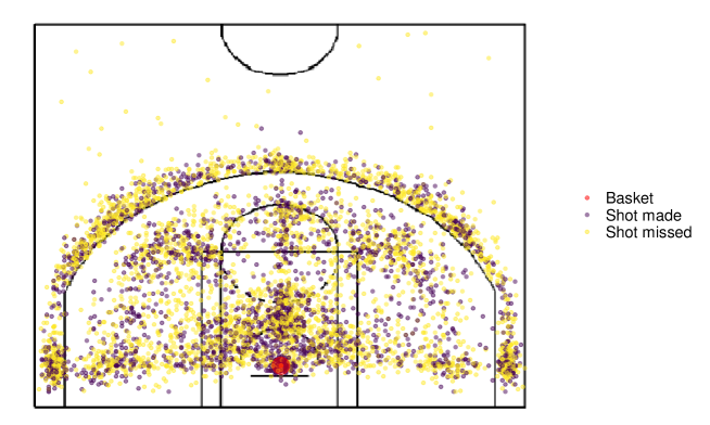
Figure 1: Shot chart of the Miami Heat during the 2005-2006 season, showing the location of shots on the court, and indicating the shot results and the exact position of the basket.

4.1 Modelling the shooting performance of the Miami Heat team

We apply the Bayesian model presented in Section (2). The sampling model is also defined in terms of the two sub-processes, one defined in terms of an HMC that accounts for the hot and cold states, and the other in terms of an observed Bernoulli longitudinal variable that assesses the success or failure of each throw in relation to the hot or cold state of the chain.

The transition probabilities of the HMC $\{Z_{in},n=1,\dots,M_{i}\}$ defined for each match $i$, $i=1,\ldots,N=105$, are expressed through the logistic mixed regression models

$$\text{logit}(p_{i}^{(CH)}\mid\boldsymbol{\theta},\boldsymbol{\psi}) ={\beta}_{CH}+b_{i}^{(CH)},$$

$$\text{logit}(p_{i}^{(HC)}\mid\boldsymbol{\theta},\boldsymbol{\psi}) ={\beta}_{HC}+b_{i}^{(HC)},$$

which express each of the two relevant probabilities, $p_{i}^{(CH)}$ and $p_{i}^{(HC)}$, in terms of an intercept common, indicating the average logit of the transition probabilities, to all matches and a specific random effect, $b_{i}^{(CH)}$ and $b_{i}^{(HC)}$, associated with the match. These random effects are mutually independent and conditionally normally distributed as $(b_{i}^{(CH)}|\sigma_{CH})\sim\text{N}(0,\sigma_{CH}^{2})$ and $(b_{i}^{(HC)}|\sigma_{HC})\sim\text{N}(0,\sigma_{HC}^{2})$. The initial probability vector $\boldsymbol{\delta}=(\delta_{C},\delta_{H})$ is also considered.

For the observed part of the sampling model, the probabilities $\gamma_{in}^{H}$ and $\gamma_{in}^{C}$ of making a basket on shot $n$ in match $i$ when the team is respectively in the hot or the cold state are described as

$$\text{logit}(\gamma_{in}^{C}) =\alpha_{C}+\alpha_{d}X_{in}+\alpha_{FT}I_{FT}(in)+a_{i},$$

$$\text{logit}(\gamma_{in}^{H}) =\alpha_{H}+\alpha_{d}X_{in}+\alpha_{FT}I_{FT}(in)+a_{i},$$

where $\alpha_{C}$ and $\alpha_{H}$ are common intercepts for the probability associated with the cold and the hot state respectively, $\alpha_{d}$ and $\alpha_{FT}$ are the regression coefficients associated with covariates $X_{in}$ and $I_{FT}(in)$ that respectively describe the distance from the basket in the $n$th shot of the game $i$ and an indicator variable that is 1 when the $n$-th shot of game $i$ is a free throw and zero otherwise. Random effects $a_{i}$ are assumed normally distributed, i. e. $(a_{i}|\sigma_{a})\sim\text{N}(0,\sigma_{a}^{2})$, and conditional independent given $\sigma_{a}$, for any $i$.

In order to complete the specification of the BLHMM model we need to elicit a prior distribution for the parameters and hyperpameters of the model. We assume prior independence within a minimally informative prior scenario. In particular, we select a beta distribution for the initial probability $\pi(\delta_{C})=\text{Be}(1,1)$, and uniform distributions for the standard deviation parameters $\pi(\sigma_{a})=\pi(\sigma_{CH})=\pi(\sigma_{HC})=\text{U}(0,10)$. For the two regression coefficients, $\alpha_{d}$ and $\alpha_{FT}$, associated with the covariates a wide normal distribution is selected, $\pi(\beta_{CH})=\pi(\beta_{HC})=\pi(\alpha_{d})=\pi(\alpha_{FT})=\text{N}(0,10^{2})$. Finally, to avoid the problem of identifiability because of the label switching issue (see among others McCulloch and Tsay,, 1994; Frühwirth-Schnatter,, 2001; Spezia,, 2009), we include the following restriction in the $\alpha_{C}$’s and $\alpha_{H}$’s prior distributions

$$\begin{split}\pi(\alpha_{C})=\pi(&\alpha_{H})=\text{N}(0,10^{2}),\,\,\alpha_{C}\leq\alpha_{H}.\end{split}$$

4.2 Posterior distribution

The complexity of the BLHMM model makes the posterior distribution analytically intractable. We approximated it by means of Markov chain Monte Carlo (MCMC) sampling methods (Tanner,, 2012) via the JAGS software (Plummer et al.,, 2003). Three parallel chains were run for $30\hskip 0.99585pt000$ iterations each after burn-ins of $30\hskip 0.99585pt000$ iterations. In addition, based on the estimated autocorrelation in the sample, and in order to reduce it, the chains were also thinned at every 30th iteration. Moreover, the full analysis, performed by an R code (R version 4.0.5), and the data are available as supplementary material at https://github.com/gcalvobayarri/hot_hand_model.git.

Table 1: Posterior summaries (mean, standard deviation, 95% credible interval and $\hat{R}$) for the parameters and hyperparameters of the Miami Heat shooting performance hot hand model.

Submodel		mean	sd	$q_{0.025}$	$q_{0.975}$	$\hat{R}$
Latent	$\beta_{CH}$	$-0.49$	$0.05$	$-0.58$	$-0.39$	$1.001$
	$\beta_{HC}$	$0.38$	$0.06$	$0.27$	$0.49$	$1.000$
	$\delta_{C}$	$0.55$	$0.06$	$0.43$	$0.68$	$1.000$
	$\sigma_{CH}$	$0.07$	$0.05$	$0.00$	$0.18$	$1.011$
	$\sigma_{HC}$	$0.10$	$0.07$	$0.00$	$0.25$	$1.048$
Observable	$\alpha_{C}$	$-0.15$	$0.07$	$-0.29$	$-0.01$	$0.999$
	$\alpha_{H}$	$12.59$	$1.19$	$10.52$	$14.97$	$1.014$
	$\alpha_{d}$	$-0.42$	$0.05$	$-0.51$	$-0.33$	$1.017$
	$\alpha_{FT}$	$6.37$	$0.69$	$5.16$	$7.75$	$1.017$
	$\sigma_{a}$	$0.15$	$0.08$	$0.00$	$0.31$	$1.024$

The posterior distribution provides useful information on the general performance of the Miami Heat team in a match. Table 1 shows the posterior summary for the parameters and hyperparameters included in the model. Furthermore, we computed a standard convergence diagnostic measure, $\hat{R}$ (Gelman et al.,, 2013), for each parameter and hyperparameter. It is noteworthy that all $\hat{R}$ values were close to 1, which indicates good convergence of the MCMC algorithm.

We focus first on the elements of the hidden model. Posterior means of the common intercepts included in the transition probabilities $\beta_{CH}$ and $\beta_{HC}$ clearly indicate a higher probability of moving from the hot state to the cold state than from the cold state to the hot state. In particular, the posterior mean (computed by Formula 7) of the probability of switching from $C$ to $H$ in a generic match is $0.38$, and from $H$ to $C$ is $0.59$. Thus, remaining in the cold state in one transition is more likely than switching to the hot, or than remaining in the hot state. This can also be observed in Figure 2, which displays the posterior distribution of the transition probabilities for a generic match. Moreover, the expected posterior probability of being in the cold state when the match starts is around $0.55$ according to the posterior mean of $\delta_{C}$.

On the other hand, for the observed Bernoulli sub-process the posterior distribution of the common intercepts $\alpha_{C}$ and $\alpha_{H}$ shows a large difference of the magnitude of $\alpha_{H}$ with respect to $\alpha_{C}$ as seen in their means E$(\alpha_{C}\mid\mathcal{D})=-0.15$ and E$(\alpha_{H}\mid\mathcal{D})=$12.59. Following the same procedure as above for the transition probabilities, we have a posterior expected probability of $0.46$ of making a shot from a distance of 0 feet to the basket when the team is in the cold state, and almost $1$ in the case of the hot state when the distance to the basket is 0.25 feet.

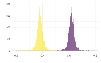
(a) ($p^{(CC)}$, $p^{(CH)}$)

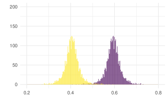
(b) ($p^{(HC)}$, $p^{(HH)}$)

Figure 2: Posterior distribution histograms (with frequencies) of the transition probabilities (a) $p^{(CC)}$ (in purple) and $p^{(CH)}$ (in yellow), and (b) $p^{(HC)}$ (in purple) and $p^{(HH)}$ (in yellow) integrating the random effects associated with the match.

The two covariates considered in the modelling are relevant. The coefficient parameter associated with the distance to the basket, $\alpha_{d}$, is completely negative, E$(\alpha_{d}\mid\mathcal{D})=$-0.42, with a small posterior standard deviation, SD$(\alpha_{d}\mid\mathcal{D})$=0.03, which means that the probability of successful shooting decreases when the distance is further away. In addition, the credible interval of the coefficient associated with the free throws has a large positive expected value, E$(\alpha_{FT}\mid\mathcal{D})=$6.37. Therefore, making a free throw looks easier than making a field goal from that distance. Finally, the random effects associated with the matches included in the success probability are also important since their associated standard deviation $\sigma_{a}$ has a posterior mean of $0.15$. It can be stated that a relevant portion of the variability can be attributed to the variations in the scoring efficiency of the team in the different games.

All information we extract from the posterior distribution provides an immense number of possibilities to assess different aspects of the performance of the team. We can discuss some of them right now.

4.2.1 Occupancy times

Occupancy times admit many different posterior outputs. We only focus here on the posterior distribution of occupancy times in the cold and the hot state in a generic match in which the team attempted $N=120$ shots. Figure 3 shows the posterior distribution of the occupancy times in the cold and the hot state in a match with $N=120$ shots and the two possibilities of initial state, cold and hot.

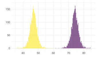
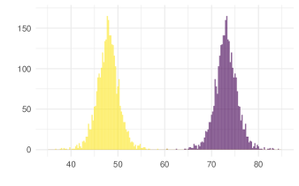
Figure 3: Posterior distribution histograms (with frequencies) of the occupancy times in the states hot (in yellow) and cold (in purple) in a match with $N=120$ shots that starts (a) in the cold and (b) in the hot state.

It is interesting to note that the team spends more time in the cold state than in the hot (with a posterior mean of 74.05 and 46.85, respectively), and that the state in which the team starts playing is practically irrelevant because there is hardly any difference between the two figures.

4.2.2 Stationary distributions

Although we could consider a stationary distribution of the chain associated with each match of the season, we focus on the posterior distribution $\pi((\Delta^{(C)},\Delta^{(H)}\mid\boldsymbol{\theta})\mid\mathcal{D})$ of the stationary distribution of the chain corresponding to a generic match. Table 2 shows a summary of the posterior distribution of the stationary distribution for the cold and hot state.

Table 2: Posterior summaries (mean, standard deviation and 95% credible interval) for the stationary distribution of the hidden Markov chain associated with a generic match.

	mean	sd	$q_{0.025}$	$q_{0.975}$
$\Delta^{(C)}$	$0.61$	$0.02$	$0.57$	$0.65$
$\Delta^{(H)}$	$0.39$	$0.02$	$0.35$	$0.43$

In summary, the probability of being in the cold state for the Miami Heat team in the 2005-2006 season was around $0.61$, so of being in the hot state it was $0.39$. Both distributions have very little variability.

4.2.3 Sojourn times

We consider a cold or a hot streak when the team stays in the same state for more than three shots. This number of shots is an arbitrary choice that can only be justified in order to illustrate the potential of our modelling to improve the understanding of the behaviour of the team. Figure 4 shows a violin plot of the posterior distribution of the probability for a cold and for a hot streak in a generic match of the Miami Heat. There, we observe the probability of a cold streak (around 0.25) is nearly three times higher than the probability of a hot streak (less than 0.1). The much smaller amplitude of the hot distribution compared to the cold one is also evident.

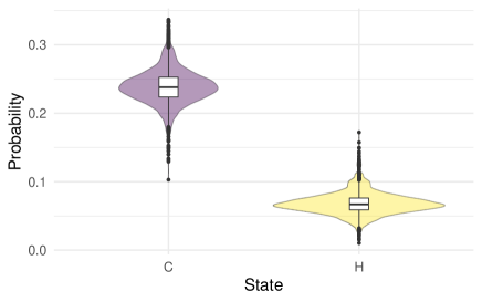
Figure 4: Violin and box plot of the posterior probability distribution for a cold and a hot streak.

4.2.4 Probability of making a basket

The probability of making a basket depends on the state the team is currently visiting, the distance to the basket at which the shot is made, and whether the shot is a free throw or not. Figure 5 shows the posterior mean and the 95% credible interval for the probability of making a basket depending on the distance at which the shot (non-free throw) is made when the team is in the cold state, hot state or in the case where the state of the team is unknown.

When the team is in the cold state, one can see that for easy shots (i.e. shots close to the basket) there is a probability of around $0.5$ of making a basket. However, from a distance of 10 feet, it is almost impossible to succeed. On the other hand, when the team is in the hot state, it is very likely to make a successful shot up to 15 feet. Then, from this distance, the probability starts to decrease slowly. Further, for a shot, in which the current state is unknown, the probability of success is also negatively related to the distance to the basket. Shots closer to the basket have a probability of success around $0.7$, whereas for intermediate shots this probability stabilises at around $0.5$. Finally, the probability of making a three-point shot drops to $0.4$.

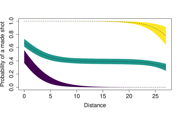
Figure 5: Posterior means and 95$\%$ credible interval for the probabilities of making a basket depending on the distance, in feet, in three different scenarios. Purple curve represents the case when the team is in the cold state, the yellow plot is for the hot state, and the green plot is the general case when the state of the team is unknown.

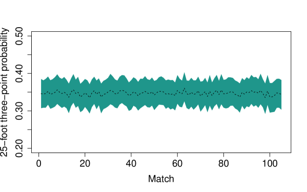
Figure 6: Posterior mean and credible interval for the probability of making a basket from 25 feet distance in the general case when the state of the team is unknown.

It can be interesting to visualise the team’s performance over the different games of the season. In that sense, Figure 6 shows the mean and the 95th percentile credible interval of the probability of hitting a shot from 25 feet, in which the team’s state is unknown, in each of the matches of the season. We observe a very marked regularity in all the games of the season, very little variability among games and a very stable behaviour in all phases of the season.

5 Conclusions

During our analysis of the Miami Heat season, we noticed something more like a cold hand instead of a hot hand. Based on our results, in any given game, the cold streaks seen to have more occurrences than hot streaks. Moreover, according to the posterior distribution of the transition probabilities, the two states are clearly differentiated: in fact, the team’s performance is very different depending on which state it is in.

Our BLHMM can be employed as a useful tool for analysing the performance of a team or a player. It could even be used to compare the performances of different teams as it provides information that is not possible to obtain with traditional modelling. It might also be used to analyse the performance of an opponent’s team during the course of a match.

Finally, for future research, the inclusion of a third intermediate state that is neither hot nor cold is an interesting possibility. In addition, the exploration of continuous-time Markov chains could be worthwhile to better model this phenomenon.

References

- Adler, (1981) Adler, P. (1981). Momentum, a Theory of Social Action: A Theory of Social Action. Sage Pubns.
- Albert and Bennett, (2001) Albert, J. and Bennett, J. (2001). Streakiness (or, The Hot Hand). In Curve Ball, pages 111–144. Springer.
- Frühwirth-Schnatter, (2001) Frühwirth-Schnatter, S. (2001). Markov chain Monte Carlo estimation of classical and dynamic switching and mixture models. Journal of the American Statistical Association, 96(453):194–209.
- Gelman et al., (2013) Gelman, A., Carlin, J. B., Stern, H. S., Dunson, D. B., Vehtari, A., and Rubin, D. B. (2013). Bayesian data analysis. CRC press.
- Gilovich et al., (1985) Gilovich, T., Vallone, R., and Tversky, A. (1985). The hot hand in basketball: On the misperception of random sequences. Cognitive psychology, 17(3):295–314.
- Kulkarni, (2016) Kulkarni, V. G. (2016). Modeling and analysis of stochastic systems. Chapman and Hall/CRC.
- McCulloch and Tsay, (1994) McCulloch, R. E. and Tsay, R. S. (1994). Statistical analysis of economic time series via Markov switching models. Journal of Time Series Analysis, 15(5):523–539.
- Miller and Sanjurjo, (2018) Miller, J. B. and Sanjurjo, A. (2018). Surprised by the hot hand fallacy? a truth in the law of small numbers. Econometrica, 86(6):2019–2047.
- NBA, (2020) NBA (2020). NBAstuffer. https://www.nbastuffer.com/analytics101/playbyplay-data/. Accessed: 2022-05-03.
- Ötting et al., (2020) Ötting, M., Langrock, R., Deutscher, C., and Leos-Barajas, V. (2020). The hot hand in professional darts. Journal of the Royal Statistical Society: Series A (Statistics in Society), 183(2):565–580.
- Plummer et al., (2003) Plummer, M. et al. (2003). Jags: A program for analysis of Bayesian graphical models using Gibbs sampling. In Proceedings of the 3rd international workshop on distributed statistical computing, volume 124. Vienna, Austria.
- Sandri et al., (2020) Sandri, M., Zuccolotto, P., and Manisera, M. (2020). Markov switching modelling of shooting performance variability and teammate interactions in basketball. Journal of the Royal Statistical Society: Series C, 69(5):1337–1356.
- Spezia, (2009) Spezia, L. (2009). Reversible jump and the label switching problem in hidden Markov models. Journal of Statistical Planning and Inference, 139(7):2305–2315.
- Sun, (2004) Sun, Y. (2004). Detecting the hot hand: An alternative model. In Proceedings of the Annual Meeting of the Cognitive Science Society, volume 26(26).
- Tanner, (2012) Tanner, M. A. (2012). Tools for Statistical Inference. Springer.
- Wetzels et al., (2016) Wetzels, R., Tutschkow, D., Dolan, C., van der Sluis, S., Dutilh, G., and Wagenmakers, E.-J. (2016). A Bayesian test for the hot hand phenomenon. Journal of Mathematical Psychology, 72:200–209.
- Zuccolotto and Manisera, (2020) Zuccolotto, P. and Manisera, M. (2020). Basketball data science: with applications in R. CRC Press.