Second Term Improvement to Generalised

Linear Mixed Model Asymptotics

By Luca Maestrini¹, Aishwarya Bhaskaran² and Matt P. Wand³

¹The Australian National University, ²Macquarie University and ³University of Technology Sydney

31st March, 2023

Abstract

A recent article on generalised linear mixed model asymptotics, Jiang et al. (2022), derived the rates of convergence for the asymptotic variances of maximum likelihood estimators. If $m$ denotes the number of groups and $n$ is the average within-group sample size then the asymptotic variances have orders $m^{-1}$ and $(mn)^{-1}$, depending on the parameter. We extend this theory to provide explicit forms of the $(mn)^{-1}$ second terms of the asymptotically harder-to-estimate parameters. Improved accuracy of studentised confidence intervals is one consequence of our theory.

Keywords: Longitudinal data analysis, Maximum likelihood estimation, Studentisation.

1 Introduction

Generalised linear mixed models are a vehicle for regression analysis of grouped data with non-Gaussian responses such as counts and categorical labels. Until recently, the precise asymptotic behaviours of the conditional maximum likelihood estimators were not known for these models. Jiang et al. (2022) derived leading term asymptotic variances and showed them have orders $m^{-1}$ and $(mn)^{-1}$, depending on the parameter, where $m$ is the number of groups and $n$ is the average within-group sample size. The main contribution of this article is to extend the asymptotic variance and covariance approximations to terms in $(mn)^{-1}$ for all parameters. This constitutes second term improvement to generalized linear mixed model asymptotics. The potential statistical payoffs are improved accuracy of confidential intervals, hypothesis tests, sample size calculations and optimal design.

The essence of generalized linear mixed models is the extension of general linear models via the addition of random effects that allow for the handling of correlations arising from repeated measures. There are numerous types of random effect structures. The most common is the two-level nested structure, corresponding to repeated measures within each of $m$ distinct groups. This version of generalised linear mixed models, with frequentist inference via maximum likelihood and its quasi-likelihood extension, is our focus here. Overviews of generalised linear mixed models are provided by books such as Jiang & Nguyen (2021), McCulloch et al. (2008) and Stroup (2013).

Suppose that a fixed effects parameter in a two-level generalised linear mixed model is accompanied by a random effect. Jiang et al. (2022) showed that the variance of its maximum likelihood estimator, conditional on the predictor data, is asymptotic to $C_{1}m^{-1}$ for some deterministic constant $C_{1}$ that depends on the true model parameter values. The crux of this article is to extend the asymptotic variance approximation to $C_{1}m^{-1}+C_{2}(mn)^{-1}$ for an additional deterministic constant $C_{2}$. We derive the explicit form of $C_{2}$ for two-level nested generalised linear mixed models for both maximum likelihood and maximum quasi-likelihood situations. Even though, in general, $C_{2}$ does not have a succinct form it is still usable in that operations such as studentisation are straightforward and result in improvements in statistical utility.

For two-level nested mixed models, $(mn)^{-1}$ is the best possible rate of convergence for the asymptotic variance of the estimator of a model parameter. Such a rate is achieved by maximum likelihood estimators of fixed effects parameters unaccompanied by random effects and dispersion parameters (e.g. Bhaskaran & Wand, 2023). The current article closes the problem of obtaining the precise asymptotic forms of the variances, up to terms in $(mn)^{-1}$, for estimation of all model parameters.

Section 2 describes the model under consideration and corresponding maximum estimators. Our second term improvement results are presented in Section 3. Section 4 describes statistical utility due to the new asymptotic results. We present some corroborating numerical results in Section 5. A supplement to this article contains derivational details.

2 Model Description and Maximum Likelihood Estimation

Consider the class of two-parameter exponential family of density, or probability mass, functions with generic form

$$p(y;\eta,\phi)=\exp[\left\{y\eta-b(\eta)+c(y)\right\}/\phi+d(y,\phi)]h(y)$$ (1)

where $\eta$ is the natural parameter and $\phi>0$ is the dispersion parameter. Examples include the Gaussian density for which $b(x)={\textstyle{\frac{1}{2}}}x^{2}$, $c(x)=-{\textstyle{\frac{1}{2}}}x^{2}$, $d(x_{1},x_{2})=-{\textstyle{\frac{1}{2}}}\log(2\pi x_{2})$ and $h(x)=I(x\in{\mathbb{R}})$ and the Gamma density function for which $b(x)=-\log(-x)$, $c(x)=\log(x)$, $d(x_{1},x_{2})=-\log(x_{1})-\log(x_{2})/x_{2}-\log\Gamma(1/x_{2})$ and $h(x)=I(x>0)$. Here $I({\mathcal{P}})=1$ if the condition ${\mathcal{P}}$ is true and $I({\mathcal{P}})=0$ if ${\mathcal{P}}$ is false. The Binomial and Poisson probability mass functions are also special cases of (1) but with $\phi$ fixed at 1. When (1) is used in regression contexts a common modelling extension for count and proportion responses, usually to account for overdispersion, is to remove the $\phi=1$ restriction and replace it with $\phi>0$. In these circumstances $\{y\eta-b(\eta)+c(y)\}/\phi+d(y,\phi)$ is labelled a quasi-likelihood function since it is not the logarithm of a probability mass function for $\phi\neq 1$. We use the more general quasi-likelihood terminology for the remainder of this article.

Consider, for observations of the random pairs $(\boldsymbol{X}_{ij},Y_{ij})$, $1\leq i\leq m$, $1\leq j\leq n_{i}$, generalised linear mixed models of the form,

$$\begin{array}[]{l}Y_{ij}|\boldsymbol{X}_{ij},\boldsymbol{U}_{i}\ \mbox{independent having quasi-likelihood function (2) with natural {\color[rgb]{0,0,0}parameter}}\\[4.30554pt] \left(\boldsymbol{\beta}^{0}+\left[\begin{array}[]{c}\boldsymbol{U}_{i}\\ \boldsymbol{0}\end{array}\right]\right)^{T}\boldsymbol{X}_{ij}\ \mbox{such that the}\ \boldsymbol{U}_{i}\ \mbox{are independent $N(\boldsymbol{0},\boldsymbol{\Sigma}^{0})$ {\color[rgb]{0,0,0}random vectors.}}\end{array}$$ (2)

The $\boldsymbol{X}_{ij}$ are $d_{\mbox{\tiny F}}\times 1$ random vectors corresponding to predictors. The $\boldsymbol{U}_{i}$ are $d_{\mbox{\tiny R}}\times 1$ unobserved random effects vectors, where $d_{\mbox{\tiny R}}\leq d_{\mbox{\tiny F}}$. Under this set-up the first $d_{\mbox{\tiny R}}$ entries of the $\boldsymbol{X}_{ij}$ are partnered by a random effect. The remaining entries correspond to predictors that have a fixed effect only. We assume that the $\boldsymbol{X}_{ij}$ and $\boldsymbol{U}_{i}$, for $1\leq i\leq m$ and $1\leq j\leq n_{i}$, are totally independent, with the $\boldsymbol{X}_{ij}$ each having the same distribution as the $d_{\mbox{\tiny F}}\times 1$ random vector $\boldsymbol{X}$ and the $\boldsymbol{U}_{i}$ each having the same distribution as the $d_{\mbox{\tiny R}}\times 1$ random vector $\boldsymbol{U}$.

For any $\boldsymbol{\beta}$ $(d_{\mbox{\tiny F}}\times 1)$ and $\boldsymbol{\Sigma}$ $(d_{\mbox{\tiny R}}\times d_{\mbox{\tiny R}})$ that is symmetric and positive definite and conditional on the $\boldsymbol{X}_{ij}$ data, the quasi-likelihood is

$$\ell(\boldsymbol{\beta},\boldsymbol{\Sigma})=\sum_{i=1}^{m}\sum_{j=1}^{n_{i}}[\{Y_{ij}(\boldsymbol{\beta}^{T}\boldsymbol{X}_{ij}+c(Y_{ij})\}/\phi+d(Y_{ij},\phi)]-\frac{m}{2}\log|2\pi\boldsymbol{\Sigma}|$$

$$\qquad\quad\quad\quad+\sum_{i=1}^{m}\log\int_{{\mathbb{R}}^{d_{\mbox{\tiny R}}}}\exp\Bigg{[}\frac{1}{\phi}\sum_{j=1}^{n_{i}}\left\{Y_{ij}\left[\begin{array}[]{c}\boldsymbol{u}\\ \boldsymbol{0}\end{array}\right]^{T}\boldsymbol{X}_{ij}-b\left(\left(\boldsymbol{\beta}+\left[\begin{array}[]{c}\boldsymbol{u}\\ \boldsymbol{0}\end{array}\right]\right)^{T}\boldsymbol{X}_{ij}\right)\right\}-{\textstyle{\frac{1}{2}}}\boldsymbol{u}^{T}\boldsymbol{\Sigma}^{-1}\boldsymbol{u}\Bigg{]}\,d\boldsymbol{u}.$$

The maximum quasi-likelihood estimator of $(\boldsymbol{\beta}^{0},\boldsymbol{\Sigma}^{0})$ is

$$({\widehat{\boldsymbol{\beta}}},{\widehat{\boldsymbol{\Sigma}}})=\mathop{\mbox{\rm argmax}}_{\boldsymbol{\beta},\boldsymbol{\Sigma}}\ell(\boldsymbol{\beta},\boldsymbol{\Sigma}).$$

Suppose that $d_{\mbox{\tiny F}}>d_{\mbox{\tiny R}}$ and consider the partition $\boldsymbol{\beta}=[\boldsymbol{\beta}_{\mbox{\scriptsize A}}^{T}\ \boldsymbol{\beta}_{\mbox{\scriptsize B}}^{T}]^{T}$ of the fixed effects parameter vector, where $\boldsymbol{\beta}_{\mbox{\scriptsize A}}$ is $d_{\mbox{\tiny R}}\times 1$ and $\boldsymbol{\beta}_{\mbox{\scriptsize B}}$ is $(d_{\mbox{\tiny F}}-d_{\mbox{\tiny R}})\times 1$. The $d_{\mbox{\tiny F}}=d_{\mbox{\tiny R}}$ boundary case is such that $\boldsymbol{\beta}_{\mbox{\scriptsize B}}$ is null. Also, let $\mathbfcal{X}\equiv\{\boldsymbol{X}_{ij}:1\leq i\leq m,\ 1\leq j\leq n_{i}\}$. Theorem 1 of Jiang et al. (2022) implies that, under some mild conditions, the covariance matrices of ${\widehat{\boldsymbol{\beta}}}_{\mbox{\scriptsize A}}$, ${\widehat{\boldsymbol{\beta}}}_{\mbox{\scriptsize B}}$ and $\mbox{\rm vech}({\widehat{\boldsymbol{\Sigma}}})$ have leading term behaviour given by

$$\mbox{\rm Cov}\big{(}{\widehat{\boldsymbol{\beta}}}_{\mbox{\scriptsize A}}|\mathbfcal{X}\big{)}=\frac{\boldsymbol{\Sigma}^{0}\{1+o_{p}(1)\}}{m},\ \ \mbox{\rm Cov}\big{(}{\widehat{\boldsymbol{\beta}}}_{\mbox{\scriptsize B}}|\mathbfcal{X}\big{)}=\frac{{\color[rgb]{0,0,0}\phi}\boldsymbol{\Lambda}_{\boldsymbol{\beta}_{\mbox{\scriptsize B}}}\{1+o_{p}(1)\}}{mn},\ \ \mbox{where}\ \ n\equiv\frac{1}{m}\sum_{i=1}^{m}n_{i},$$ (4)

and

$$\mbox{\rm Cov}\big{(}\mbox{\rm vech}({\widehat{\boldsymbol{\Sigma}}})|\mathbfcal{X}\big{)}=\frac{2\boldsymbol{D}_{d_{\mbox{\tiny R}}}^{+}(\boldsymbol{\Sigma}^{0}\otimes\boldsymbol{\Sigma}^{0})\boldsymbol{D}_{d_{\mbox{\tiny R}}}^{+T}\{1+o_{p}(1)\}}{m}.$$ (5)

Here $\boldsymbol{\Lambda}_{\boldsymbol{\beta}_{\mbox{\scriptsize B}}}$ is a $(d_{\mbox{\tiny F}}-d_{\mbox{\tiny R}})\times(d_{\mbox{\tiny F}}-d_{\mbox{\tiny R}})$ matrix that depends on $\boldsymbol{\beta}$ and the $(\boldsymbol{X},\boldsymbol{U})$ distribution, $\boldsymbol{D}_{d_{\mbox{\tiny R}}}$ is the matrix of zeroes and ones such that $\boldsymbol{D}_{d_{\mbox{\tiny R}}}\mbox{\rm vech}(\boldsymbol{A})=\mbox{\rm vec}(\boldsymbol{A})$ for all $d_{\mbox{\tiny R}}\times d_{\mbox{\tiny R}}$ symmetric matrices $\boldsymbol{A}$ and $\boldsymbol{D}_{d_{\mbox{\tiny R}}}^{+}=(\boldsymbol{D}_{d_{\mbox{\tiny R}}}^{T}\boldsymbol{D}_{d_{\mbox{\tiny R}}})^{-1}\boldsymbol{D}_{d_{\mbox{\tiny R}}}^{T}$ is the Moore-Penrose inverse of $\boldsymbol{D}_{d_{\mbox{\tiny R}}}$. The theory of Jiang et al. (2022) also indicates a degree of asymptotic orthogonality between $\boldsymbol{\beta}_{\mbox{\scriptsize A}}$ and $\boldsymbol{\beta}_{\mbox{\scriptsize B}}$ in that $E\big{\{}({\widehat{\boldsymbol{\beta}}}_{\mbox{\scriptsize A}}-\boldsymbol{\beta}_{\mbox{\scriptsize A}}^{0})({\widehat{\boldsymbol{\beta}}}_{\mbox{\scriptsize B}}-\boldsymbol{\beta}_{\mbox{\scriptsize B}}^{0})^{T}|\mathbfcal{X}\big{\}}$ has $O_{p}\{(mn)^{-1}\}$ entries, which implies that the correlations between the entries of ${\widehat{\boldsymbol{\beta}}}_{\mbox{\scriptsize A}}$ and ${\widehat{\boldsymbol{\beta}}}_{\mbox{\scriptsize B}}$ are asymptotically negligible.

The leading term approximations of the variability in ${\widehat{\boldsymbol{\beta}}}_{\mbox{\scriptsize A}}$ and $\mbox{\rm vech}({\widehat{\boldsymbol{\Sigma}}})$, given by (4) and (5), are somewhat crude. Unlike the asymptotic covariance of ${\widehat{\boldsymbol{\beta}}}_{\mbox{\scriptsize B}}$, they do not show the effect of the average within-group sample size $n$. In the next section we investigate their second term improvements.

3 Two-Term Asymptotic Covariance Results

We define the two-term asymptotic covariance matrix problem to be the determination of the unique deterministic matrices $\boldsymbol{M}_{{\hbox{\hbox to0.0pt{$\scriptstyle{\beta}$\hss}\kern 0.25pt\hbox to0.0pt{$\scriptstyle{\beta}$\hss}\kern 0.25pt$\scriptstyle{\beta}$}}}$ and $\boldsymbol{M}_{{\hbox{\hbox to0.0pt{$\scriptstyle{\Sigma}$\hss}\kern 0.25pt\hbox to0.0pt{$\scriptstyle{\Sigma}$\hss}\kern 0.25pt$\scriptstyle{\Sigma}$}}}$ such that

$$\mbox{\rm Cov}\big{(}{\widehat{\boldsymbol{\beta}}}|\mathbfcal{X}\big{)} = \frac{1}{m}\left[\begin{array}[]{cc}\boldsymbol{\Sigma}^{0}&\quad\boldsymbol{O}\\[4.30554pt] \boldsymbol{O}&\quad\boldsymbol{O}\end{array}\right]+\frac{\boldsymbol{M}_{{\hbox{\hbox to0.0pt{$\scriptstyle{\beta}$\hss}\kern 0.25pt\hbox to0.0pt{$\scriptstyle{\beta}$\hss}\kern 0.25pt$\scriptstyle{\beta}$}}}\{1+o_{p}(1)\}}{mn}\quad\mbox{and}$$

$$\mbox{\rm Cov}\big{(}\mbox{\rm vech}({\widehat{\boldsymbol{\Sigma}}})|\mathbfcal{X}\big{)} = \displaystyle{\frac{2\boldsymbol{D}_{d_{\mbox{\tiny R}}}^{+}(\boldsymbol{\Sigma}^{0}\otimes\boldsymbol{\Sigma}^{0})\boldsymbol{D}_{d_{\mbox{\tiny R}}}^{+T}}{m}}+\frac{\boldsymbol{M}_{{\hbox{\hbox to0.0pt{$\scriptstyle{\Sigma}$\hss}\kern 0.25pt\hbox to0.0pt{$\scriptstyle{\Sigma}$\hss}\kern 0.25pt$\scriptstyle{\Sigma}$}}}\{1+o_{p}(1)\}}{mn}$$

under reasonably mild conditions.

An example for which a solution to the two-term asymptotic covariance problem can be expressed relatively simply is the $d_{\mbox{\tiny F}}=2$, $d_{\mbox{\tiny R}}=1$ Poisson quasi-likelihood special case of (2), with parameters

$$\boldsymbol{\beta}=(\beta_{0},\beta_{1})\quad\mbox{and}\quad\boldsymbol{\Sigma}=\sigma^{2}\quad\mbox{and predictor variable}\quad\boldsymbol{X}=\left[\begin{array}[]{c}1\\[4.30554pt] X\end{array}\right]$$

for a scalar random variable $X$. Define

$$a_{1}\big{(}\beta_{0},\beta_{1},\sigma^{2}\big{)}\equiv e^{\beta_{0}+\sigma^{2}/2}\big{[}E(X^{2}e^{\beta_{1}X})E(e^{\beta_{1}X})-\{E(Xe^{\beta_{1}X})\}^{2}\big{]}$$

and

$$a_{2}(\beta_{1},\sigma^{2})\equiv\frac{e^{\sigma^{2}}E\big{(}X^{2}e^{\beta_{1}X}\big{)}E\big{(}e^{\beta_{1}X}\big{)}+\big{(}1-e^{\sigma^{2}}\big{)}E\{\big{(}Xe^{\beta_{1}X}\big{)}\}^{2}}{E\big{(}e^{\beta_{1}X}\big{)}}.$$

Then the two-term covariance matrix of $({\widehat{\beta}}_{0},{\widehat{\beta}}_{1})$ is

$$\mbox{\rm Cov}\left(\left[\begin{array}[]{c}{\widehat{\beta}}_{0}\\[4.30554pt] {\widehat{\beta}}_{1}\end{array}\right]\Bigg{|}\mathbfcal{X}\right)=\frac{1}{m}\left[\begin{array}[]{cc}(\sigma^{2})^{0}&\ 0\\[4.30554pt] 0&\ 0\end{array}\right]+\frac{\phi\{1+o_{p}(1)\}}{a_{1}\big{(}\beta_{0}^{0},\beta_{1}^{0},(\sigma^{2})^{0}\big{)}\,mn}\left[\begin{array}[]{cc}a_{2}\big{(}\beta_{1}^{0},(\sigma^{2})^{0}\big{)}&\ -E\big{(}Xe^{\beta_{1}^{0}X}\big{)}\\[4.30554pt] -E\big{(}Xe^{\beta_{1}^{0}X}\big{)}&\ E\big{(}e^{\beta_{1}^{0}X}\big{)}\end{array}\right].$$

In other words, for this simple example, the solution for $\boldsymbol{M}_{{\hbox{\hbox to0.0pt{$\scriptstyle{\beta}$\hss}\kern 0.25pt\hbox to0.0pt{$\scriptstyle{\beta}$\hss}\kern 0.25pt$\scriptstyle{\beta}$}}}$ is

$$\boldsymbol{M}_{{\hbox{\hbox to0.0pt{$\scriptstyle{\beta}$\hss}\kern 0.25pt\hbox to0.0pt{$\scriptstyle{\beta}$\hss}\kern 0.25pt$\scriptstyle{\beta}$}}}=\frac{\phi}{a_{1}\big{(}\beta_{0}^{0},\beta_{1}^{0},(\sigma^{2})^{0}\big{)}}\left[\begin{array}[]{cc}a_{2}\big{(}\beta_{1}^{0},(\sigma^{2})^{0}\big{)}&\quad-E\big{(}Xe^{\beta_{1}^{0}X}\big{)}\\[4.30554pt] -E\big{(}Xe^{\beta_{1}^{0}X}\big{)}&\quad E\big{(}e^{\beta_{1}^{0}X}\big{)}\end{array}\right].$$

Studentisation of the two-term asymptotic covariance matrix for obtaining confidence intervals and Wald hypothesis tests is straightforward. For example, $E(X^{2}e^{\beta_{1}^{0}X})$ can be replaced by the estimator

$$\frac{1}{mn}\sum_{i=1}^{m}\sum_{j=1}^{n_{i}}X_{ij}^{2}e^{{\widehat{\beta}}_{1}X_{ij}}.$$

This practical aspect is discussed in depth in Section 4.

The remainder of this section is concerned with the theoretical problem of obtaining the forms of $\boldsymbol{M}_{{\hbox{\hbox to0.0pt{$\scriptstyle{\beta}$\hss}\kern 0.25pt\hbox to0.0pt{$\scriptstyle{\beta}$\hss}\kern 0.25pt$\scriptstyle{\beta}$}}}$ and $\boldsymbol{M}_{{\hbox{\hbox to0.0pt{$\scriptstyle{\Sigma}$\hss}\kern 0.25pt\hbox to0.0pt{$\scriptstyle{\Sigma}$\hss}\kern 0.25pt$\scriptstyle{\Sigma}$}}}$ for model (2) in general. The achievement of this goal has turned out to be quite challenging. The score asymptotic approximation approach used in Jiang et al. (2022) requires higher numbers of terms to obtain valid two-term covariance matrix approximations. Some of these terms can only be expressed using three-dimensional arrays rather than with matrices. Succinct statement of $\boldsymbol{M}_{{\hbox{\hbox to0.0pt{$\scriptstyle{\beta}$\hss}\kern 0.25pt\hbox to0.0pt{$\scriptstyle{\beta}$\hss}\kern 0.25pt$\scriptstyle{\beta}$}}}$ and $\boldsymbol{M}_{{\hbox{\hbox to0.0pt{$\scriptstyle{\Sigma}$\hss}\kern 0.25pt\hbox to0.0pt{$\scriptstyle{\Sigma}$\hss}\kern 0.25pt$\scriptstyle{\Sigma}$}}}$ is only possible with well-designed nested function notation. A novel notation for multiplicative combining of three-dimensional arrays with compatible matrices is also beneficial. The next subsection focusses on these notational aspects.

3.1 Notation for the Main Result

Let $\mathbfcal{A}$ be a $d_{1}\times d_{2}\times d_{3}$ array and $\boldsymbol{M}$ be a $d_{1}\times d_{2}$ matrix. Then we let

$$\mathbfcal{A}\bigstar\boldsymbol{M}\quad\mbox{denote the $d_{3}\times 1$ vector with $t$th entry given by}\quad\sum_{r=1}^{d_{1}}\sum_{s=1}^{d_{2}}(\mathbfcal{A})_{rst}(\boldsymbol{M})_{rs}.$$ (7)

Next, for $\boldsymbol{U}\sim N(\boldsymbol{0},\boldsymbol{\Sigma}^{0})$, define

$$\boldsymbol{\Omega}_{\mbox{\tiny AA}}(\boldsymbol{U})\equiv E\Big{\{}b^{\prime\prime}\big{(}(\boldsymbol{\beta}_{\mbox{\scriptsize A}}^{0}+\boldsymbol{U})^{T}\boldsymbol{X}_{\mbox{\scriptsize A}}+(\boldsymbol{\beta}_{\mbox{\scriptsize B}}^{0})^{T}\boldsymbol{X}_{\mbox{\scriptsize B}}\big{)}\boldsymbol{X}_{\mbox{\scriptsize A}}\boldsymbol{X}_{\mbox{\scriptsize A}}^{T}|\boldsymbol{U}\Big{\}},$$

$$\boldsymbol{\Omega}_{\mbox{\tiny AB}}(\boldsymbol{U})\equiv E\Big{\{}b^{\prime\prime}\big{(}(\boldsymbol{\beta}_{\mbox{\scriptsize A}}^{0}+\boldsymbol{U})^{T}\boldsymbol{X}_{\mbox{\scriptsize A}}+(\boldsymbol{\beta}_{\mbox{\scriptsize B}}^{0})^{T}\boldsymbol{X}_{\mbox{\scriptsize B}}\big{)}\boldsymbol{X}_{\mbox{\scriptsize A}}\boldsymbol{X}_{\mbox{\scriptsize B}}^{T}|\boldsymbol{U}\Big{\}}$$

and

$$\boldsymbol{\Omega}_{\mbox{\tiny BB}}(\boldsymbol{U})\equiv E\Big{\{}b^{\prime\prime}\big{(}(\boldsymbol{\beta}_{\mbox{\scriptsize A}}^{0}+\boldsymbol{U})^{T}\boldsymbol{X}_{\mbox{\scriptsize A}}+(\boldsymbol{\beta}_{\mbox{\scriptsize B}}^{0})^{T}\boldsymbol{X}_{\mbox{\scriptsize B}}\big{)}\boldsymbol{X}_{\mbox{\scriptsize B}}\boldsymbol{X}_{\mbox{\scriptsize B}}^{T}|\boldsymbol{U}\Big{\}}.$$

Also let $\boldsymbol{\Omega}^{\prime}_{\mbox{\tiny AAA}}(\boldsymbol{U})$ be the $d_{\mbox{\tiny R}}\times d_{\mbox{\tiny R}}\times d_{\mbox{\tiny R}}$ array with $(r,s,t)$ entry equal to

$$E\Big{\{}b^{\prime\prime\prime}\big{(}(\boldsymbol{\beta}_{\mbox{\scriptsize A}}^{0}+\boldsymbol{U})^{T}\boldsymbol{X}_{\mbox{\scriptsize A}}+(\boldsymbol{\beta}_{\mbox{\scriptsize B}}^{0})^{T}\boldsymbol{X}_{\mbox{\scriptsize B}}\big{)}(\boldsymbol{X}_{\mbox{\scriptsize A}})_{r}(\boldsymbol{X}_{\mbox{\scriptsize A}})_{s}(\boldsymbol{X}_{\mbox{\scriptsize A}})_{t}|\boldsymbol{U}\Big{\}}.$$

and $\boldsymbol{\Omega}^{\prime}_{\mbox{\tiny AAB}}(\boldsymbol{U})$ be the $d_{\mbox{\tiny R}}\times d_{\mbox{\tiny R}}\times(d_{\mbox{\tiny F}}-d_{\mbox{\tiny R}})$ array with $(r,s,t)$ entry equal to

$$E\Big{\{}b^{\prime\prime\prime}\big{(}(\boldsymbol{\beta}_{\mbox{\scriptsize A}}^{0}+\boldsymbol{U})^{T}\boldsymbol{X}_{\mbox{\scriptsize A}}+(\boldsymbol{\beta}_{\mbox{\scriptsize B}}^{0})^{T}\boldsymbol{X}_{\mbox{\scriptsize B}}\big{)}(\boldsymbol{X}_{\mbox{\scriptsize A}})_{r}(\boldsymbol{X}_{\mbox{\scriptsize A}})_{s}(\boldsymbol{X}_{\mbox{\scriptsize B}})_{t}\big{|}\boldsymbol{U}\Big{\}}.$$

Define the random vectors:

$$\psi_{1}(\boldsymbol{U}) \equiv \mbox{\rm vech}(\boldsymbol{\Sigma}-\boldsymbol{U}\boldsymbol{U}^{T}),\quad\psi_{2}(\boldsymbol{U})\equiv\boldsymbol{\Omega}^{\prime}_{\mbox{\tiny AAA}}(\boldsymbol{U})\bigstar\boldsymbol{\Omega}_{\mbox{\tiny AA}}(\boldsymbol{U})^{-1},$$

$$\psi_{3}(\boldsymbol{U}) \equiv \boldsymbol{\Omega}^{\prime}_{\mbox{\tiny AAB}}(\boldsymbol{U})\bigstar\boldsymbol{\Omega}_{\mbox{\tiny AA}}(\boldsymbol{U})^{-1}\ \ \mbox{and}\ \ \psi_{4}(\boldsymbol{U})\equiv\boldsymbol{D}_{d_{\mbox{\tiny R}}}^{+}\mbox{\rm vec}\Big{(}\boldsymbol{\Omega}_{\mbox{\tiny AA}}(\boldsymbol{U})^{-1}\boldsymbol{\Sigma}^{-1}\big{\{}\boldsymbol{\Sigma}-\boldsymbol{U}\boldsymbol{U}^{T}-\boldsymbol{\Sigma}\psi_{2}(\boldsymbol{U})\boldsymbol{U}^{T}\big{\}}\Big{)}.$$

Then define the random matrices:

$$\boldsymbol{\Psi}_{5}(\boldsymbol{U}) \equiv \boldsymbol{\Omega}_{\mbox{\tiny AA}}(\boldsymbol{U})^{-1}\boldsymbol{\Omega}_{\mbox{\tiny AB}}(\boldsymbol{U}),\quad\boldsymbol{\Psi}_{6}(\boldsymbol{U})\equiv\boldsymbol{\Omega}_{\mbox{\tiny BB}}(\boldsymbol{U})-\boldsymbol{\Psi}_{5}(\boldsymbol{U})^{T}\boldsymbol{\Omega}_{\mbox{\tiny AB}}(\boldsymbol{U}),$$

$$\boldsymbol{\Psi}_{7}(\boldsymbol{U}) \equiv \boldsymbol{U}\boldsymbol{U}^{T}\boldsymbol{\Sigma}^{-1}\boldsymbol{\Omega}_{\mbox{\tiny AA}}(\boldsymbol{U})^{-1},\quad\boldsymbol{\Psi}_{8}(\boldsymbol{U})\equiv\boldsymbol{D}_{d_{\mbox{\tiny R}}}^{+}\big{[}(\boldsymbol{U}\boldsymbol{U}^{T})\otimes\{\boldsymbol{\Omega}_{\mbox{\tiny AA}}(\boldsymbol{U})^{-1}\}\big{]}\boldsymbol{D}_{d_{\mbox{\tiny R}}}^{+T},$$

$$\quad\mbox{and}\quad\boldsymbol{\Psi}_{9}(\boldsymbol{U}) \equiv \psi_{1}(\boldsymbol{U})\psi_{4}(\boldsymbol{U})^{T}+\psi_{4}(\boldsymbol{U})\psi_{1}(\boldsymbol{U})^{T}.$$

Lastly, define the expectation matrices:

$$\boldsymbol{\Lambda}_{\mbox{\tiny AA}} \equiv E\Big{\{}\boldsymbol{\Psi}_{7}(\boldsymbol{U})+\boldsymbol{\Psi}_{7}(\boldsymbol{U})^{T}-\boldsymbol{\Omega}_{\mbox{\tiny AA}}(\boldsymbol{U})^{-1}+\boldsymbol{\Omega}_{\mbox{\tiny AA}}(\boldsymbol{U})^{-1}\psi_{2}(\boldsymbol{U})\boldsymbol{U}^{T}+\boldsymbol{U}\psi_{2}(\boldsymbol{U})^{T}\boldsymbol{\Omega}_{\mbox{\tiny AA}}(\boldsymbol{U})^{-1}\Big{\}},$$

$$\boldsymbol{\Lambda}_{\mbox{\tiny AB}} \equiv E\Big{\{}\boldsymbol{U}\boldsymbol{U}^{T}\boldsymbol{\Sigma}^{-1}\boldsymbol{\Psi}_{5}(\boldsymbol{U})+\boldsymbol{U}\psi_{2}(\boldsymbol{U})^{T}\boldsymbol{\Psi}_{5}(\boldsymbol{U})-\boldsymbol{U}\psi_{3}(\boldsymbol{U})^{T}\Big{\}}\quad\mbox{and}$$

$$\boldsymbol{\Phi} \equiv E\Big{(}\Big{[}\boldsymbol{\Psi}_{5}(\boldsymbol{U})^{T}\big{\{}\boldsymbol{\Sigma}^{-1}\boldsymbol{U}+\psi_{2}(\boldsymbol{U})\big{\}}-\psi_{3}(\boldsymbol{U})\Big{]}\psi_{1}(\boldsymbol{U})^{T}\Big{)}.$$

3.2 Assumptions for the Main Result

The main result depends on the following sample size asymptotic assumptions:

• The number of groups $m$ diverges to $\infty$.

• The within-group sample sizes $n_{i}$ diverge to $\infty$ in such a way that $n_{i}/n\to C_{i}$ for constants $0<C_{i}<\infty$, $1\leq i\leq m$.

• The ratio $n/m$ converges to zero.

The last of these conditions is in keeping with the number of groups being large compared with the within-group sample sizes, as often arises in practice. For our asymptotics it ensures that, for the harder-to-estimate parameters, the asymptotic variances of the maximum likelihood estimators have leading terms of the form $C_{1}m^{-1}+C_{2}(mn)^{-1}$. In addition, it ensures that the Fisher information is sufficiently dominant for obtaining asymptotic variances.

We also assume that the $(\boldsymbol{X},\boldsymbol{U})$ joint distribution is such that all required convergence in probability limits that appear in the deterministic order $(mn)^{-1}$ terms are justified. An example of such a convergence in probability statement is

$$\begin{array}[]{c}{\displaystyle\frac{1}{n}}E\Big{(}{\mathcal{H}}_{\mbox{\scriptsize AB}i}^{T}{\mathcal{H}}_{\mbox{\scriptsize AA}i}^{-1}{\mathcal{H}}_{\mbox{\scriptsize AB}i}\Big{|}\boldsymbol{X}_{i}\Big{)}\stackrel{{\scriptstyle p}}{{\to}}\boldsymbol{\Omega}_{\mbox{\tiny AB}}(\boldsymbol{U})^{T}\boldsymbol{\Omega}_{\mbox{\tiny AA}}(\boldsymbol{U})^{-1}\boldsymbol{\Omega}_{\mbox{\tiny AB}}(\boldsymbol{U})\\[4.30554pt] \mbox{where}\ {\mathcal{H}}_{\mbox{\scriptsize AA}i}\equiv{\displaystyle\sum_{j=1}^{n_{i}}}b^{\prime\prime}\big{(}(\boldsymbol{\beta}_{\mbox{\scriptsize A}}+\boldsymbol{U}_{i})^{T}\boldsymbol{X}_{\mbox{\scriptsize A}ij}+\boldsymbol{\beta}_{\mbox{\scriptsize B}}^{T}\boldsymbol{X}_{\mbox{\scriptsize B}ij}\big{)}\boldsymbol{X}_{\mbox{\scriptsize A}ij}\boldsymbol{X}_{\mbox{\scriptsize A}ij}^{T}\\[4.30554pt] \mbox{and}\ {\mathcal{H}}_{\mbox{\scriptsize AB}i}\equiv{\displaystyle\sum_{j=1}^{n_{i}}}b^{\prime\prime}\big{(}(\boldsymbol{\beta}_{\mbox{\scriptsize A}}+\boldsymbol{U}_{i})^{T}\boldsymbol{X}_{\mbox{\scriptsize A}ij}+\boldsymbol{\beta}_{\mbox{\scriptsize B}}^{T}\boldsymbol{X}_{\mbox{\scriptsize B}ij}\big{)}\boldsymbol{X}_{\mbox{\scriptsize A}ij}\boldsymbol{X}_{\mbox{\scriptsize B}ij}^{T}.\end{array}$$ (8)

Assumption (A3) of Jiang et al. (2022) provides a moment-type condition that is sufficient for (8) to hold. Also, we assume that the tail behaviour of the $(\boldsymbol{X},\boldsymbol{U})$ distribution is such that statements concerning the $o_{p}\{(mn)^{-1}\}$ remainder terms are valid. The determination of sufficient conditions on the $(\boldsymbol{X},\boldsymbol{U})$ distribution that guarantee the validity of the main result is a tall order, and beyond the scope of this article.

3.3 Statement of the Main Result

Using the notation presented in Section 3.1 and under the assumptions described in Section 3.2, and assuming $d_{\mbox{\tiny F}}>d_{\mbox{\tiny R}}$ we have

$${\begin{array}[]{l}\mbox{\rm Cov}\big{(}{\widehat{\boldsymbol{\beta}}}|\mathbfcal{X}\big{)}=\displaystyle{\frac{1}{m}}\left[\begin{array}[]{cc}\ \boldsymbol{\Sigma}^{0}&\ \ \ \boldsymbol{O}\\[4.30554pt] \boldsymbol{O}&\ \ \ \boldsymbol{O}\end{array}\right]+\displaystyle{\frac{\phi}{mn}}\left[\begin{array}[]{cc}\boldsymbol{\Lambda}_{\mbox{\tiny AA}}^{-1}&\quad\boldsymbol{\Lambda}_{\mbox{\tiny AA}}^{-1}\boldsymbol{\Lambda}_{\mbox{\tiny AB}}\\[8.61108pt] \boldsymbol{\Lambda}_{\mbox{\tiny AB}}^{T}\boldsymbol{\Lambda}_{\mbox{\tiny AA}}^{-1}&\quad\boldsymbol{\Lambda}_{\mbox{\tiny AB}}^{T}\boldsymbol{\Lambda}_{\mbox{\tiny AA}}^{-1}\boldsymbol{\Lambda}_{\mbox{\tiny AB}}+E\big{\{}\boldsymbol{\Psi}_{6}(\boldsymbol{U})\big{\}}\end{array}\right]^{-1}\{1+o_{p}(1)\}\quad\mbox{and}\\[25.83325pt] \mbox{\rm Cov}\big{(}\mbox{\rm vech}({\widehat{\boldsymbol{\Sigma}}})|\mathbfcal{X}\big{)}=\displaystyle{\frac{2\boldsymbol{D}_{d_{\mbox{\tiny R}}}^{+}(\boldsymbol{\Sigma}^{0}\otimes\boldsymbol{\Sigma}^{0})\boldsymbol{D}_{d_{\mbox{\tiny R}}}^{+T}}{m}}\\[8.61108pt] \qquad\qquad\qquad\qquad\quad\qquad+\displaystyle{\frac{\phi}{mn}}{\color[rgb]{0,0,0}\Big{(}}2E\big{\{}\boldsymbol{\Psi}_{9}(\boldsymbol{U})-2\boldsymbol{\Psi}_{8}(\boldsymbol{U})\big{\}}+\boldsymbol{\Phi}^{T}{\color[rgb]{0,0,0}\big{[}}E\{\boldsymbol{\Psi}_{6}(\boldsymbol{U})\}{\color[rgb]{0,0,0}\big{]}}^{-1}\boldsymbol{\Phi}{\color[rgb]{0,0,0}\Big{)}}\{1+o_{p}(1)\}.\end{array}}$$ (9)

For the $d_{\mbox{\tiny F}}=d_{\mbox{\tiny R}}$ boundary case the first term of $\mbox{\rm Cov}\big{(}{\widehat{\boldsymbol{\beta}}}|\mathbfcal{X}\big{)}$ is simply $\frac{1}{m}\boldsymbol{\Sigma}^{0}$.

A supplement to this article contains a full derivation of (9).

3.3.1 The Gaussian Response Special Case

In the Gaussian response special case we have $b^{\prime\prime}(x)=1$ and $b^{\prime\prime\prime}(x)=0$ and the main result reduces to the following succinct form:

$${\begin{array}[]{rcl}\mbox{\rm Cov}\big{(}{\widehat{\boldsymbol{\beta}}}|\mathbfcal{X}\big{)}&=&\displaystyle{\frac{1}{m}}\left[\begin{array}[]{cc}\boldsymbol{\Sigma}^{0}&\quad\boldsymbol{O}\\[4.30554pt] \boldsymbol{O}&\quad\boldsymbol{O}\end{array}\right]+\displaystyle{\frac{\phi\big{\{}E(\boldsymbol{X}\boldsymbol{X}^{T})\big{\}}^{-1}\{1+o_{p}(1)\}}{mn}}\quad\mbox{and}\\[21.52771pt] \mbox{\rm Cov}\big{(}\mbox{\rm vech}({\widehat{\boldsymbol{\Sigma}}})|\mathbfcal{X}\big{)}&=&\displaystyle{\frac{2\boldsymbol{D}_{d_{\mbox{\tiny R}}}^{+}(\boldsymbol{\Sigma}^{0}\otimes\boldsymbol{\Sigma}^{0})\boldsymbol{D}_{d_{\mbox{\tiny R}}}^{+T}}{m}}\\[8.61108pt] &&\qquad\qquad+\displaystyle{\frac{4\phi\boldsymbol{D}_{d_{\mbox{\tiny R}}}^{+}\big{[}\boldsymbol{\Sigma}^{0}\otimes\{E(\boldsymbol{X}_{\mbox{\scriptsize A}}\boldsymbol{X}_{\mbox{\scriptsize A}}^{T})\}^{-1}\big{]}\boldsymbol{D}_{d_{\mbox{\tiny R}}}^{+T}\{1+o_{p}(1)\}}{mn}}.\end{array}}$$ (10)

We are not aware of any previous appearances of (10) in the wider linear mixed model literature.

4 Utility of the Second Term Improvements

We now describe the utility of (9) in statistical contexts such as inference and design. Improved confidence intervals is a particularly straightforward application, which we treat next.

4.1 Confidence Intervals

For any $\boldsymbol{u}\in{\mathbb{R}}^{d_{\mbox{\tiny R}}}$, define

$${\begin{array}[]{rcl}{\widehat{\boldsymbol{\Omega}}}_{\mbox{\tiny AA}}(\boldsymbol{u})&\equiv&{\displaystyle\frac{1}{mn}\sum_{i=1}^{m}\sum_{j=1}^{n_{i}}}b^{\prime\prime}\Big{(}({\widehat{\boldsymbol{\beta}}}_{\mbox{\scriptsize A}}+\boldsymbol{u})^{T}\boldsymbol{X}_{\mbox{\scriptsize A}ij}+{\widehat{\boldsymbol{\beta}}}_{\mbox{\scriptsize B}}^{T}\boldsymbol{X}_{\mbox{\scriptsize B}ij}\Big{)}\boldsymbol{X}_{\mbox{\scriptsize A}ij}\boldsymbol{X}_{\mbox{\scriptsize A}ij}^{T},\\[4.30554pt] {\widehat{\boldsymbol{\Omega}}}_{\mbox{\tiny AB}}(\boldsymbol{u})&\equiv&{\displaystyle\frac{1}{mn}\sum_{i=1}^{m}\sum_{j=1}^{n_{i}}}b^{\prime\prime}\Big{(}({\widehat{\boldsymbol{\beta}}}_{\mbox{\scriptsize A}}+\boldsymbol{u})^{T}\boldsymbol{X}_{\mbox{\scriptsize A}ij}+{\widehat{\boldsymbol{\beta}}}_{\mbox{\scriptsize B}}^{T}\boldsymbol{X}_{\mbox{\scriptsize B}ij}\Big{)}\boldsymbol{X}_{\mbox{\scriptsize A}ij}\boldsymbol{X}_{\mbox{\scriptsize B}ij}^{T}\\[4.30554pt] \mbox{and}\quad{\widehat{\boldsymbol{\Omega}}}_{\mbox{\tiny BB}}(\boldsymbol{u})&\equiv&{\displaystyle\frac{1}{mn}\sum_{i=1}^{m}\sum_{j=1}^{n_{i}}}b^{\prime\prime}\Big{(}({\widehat{\boldsymbol{\beta}}}_{\mbox{\scriptsize A}}+\boldsymbol{u})^{T}\boldsymbol{X}_{\mbox{\scriptsize A}ij}+{\widehat{\boldsymbol{\beta}}}_{\mbox{\scriptsize B}}^{T}\boldsymbol{X}_{\mbox{\scriptsize B}ij}\Big{)}\boldsymbol{X}_{\mbox{\scriptsize B}ij}\boldsymbol{X}_{\mbox{\scriptsize B}ij}^{T}.\end{array}}$$ (11)

Then the natural studentisation of $E\big{\{}\boldsymbol{\Psi}_{6}(\boldsymbol{U})\big{\}}$ is

$${\begin{array}[]{rcl}\widehat{E}\big{\{}\boldsymbol{\Psi}_{6}(\boldsymbol{U})\big{\}}&\equiv&E\Big{\{}{\widehat{\boldsymbol{\Omega}}}_{\mbox{\tiny BB}}(\boldsymbol{U})-{\widehat{\boldsymbol{\Omega}}}_{\mbox{\tiny AB}}(\boldsymbol{U})^{T}{\widehat{\boldsymbol{\Omega}}}_{\mbox{\tiny AA}}(\boldsymbol{U})^{-1}{\widehat{\boldsymbol{\Omega}}}_{\mbox{\tiny AB}}(\boldsymbol{U})\big{|}\mathbfcal{X}\Big{\}}\\[8.61108pt] &=&|2\pi{\widehat{\boldsymbol{\Sigma}}}|^{-1/2}{\displaystyle\int_{d_{\mbox{\tiny R}}}}\Big{\{}{\widehat{\boldsymbol{\Omega}}}_{\mbox{\tiny BB}}(\boldsymbol{u})-{\widehat{\boldsymbol{\Omega}}}_{\mbox{\tiny AB}}(\boldsymbol{u})^{T}{\widehat{\boldsymbol{\Omega}}}_{\mbox{\tiny AA}}(\boldsymbol{u})^{-1}{\widehat{\boldsymbol{\Omega}}}_{\mbox{\tiny AB}}(\boldsymbol{u})\Big{\}}\exp\Big{(}-{\textstyle{\frac{1}{2}}}\boldsymbol{u}^{T}{\widehat{\boldsymbol{\Sigma}}}\boldsymbol{u}\Big{)}\,d\boldsymbol{u}.\end{array}}$$ (12)

In the last expression of (12) integration is applied element-wise to each entry of the matrix inside the integral. The natural studentisations of

$$\boldsymbol{\Lambda}_{\mbox{\tiny AA}},\quad\boldsymbol{\Lambda}_{\mbox{\tiny AB}},\quad\boldsymbol{\Phi},\quad E\big{\{}\boldsymbol{\Psi}_{8}(\boldsymbol{U})\big{\}}\quad\mbox{and}\quad E\big{\{}\boldsymbol{\Psi}_{9}(\boldsymbol{U})\big{\}}$$ (13)

are analogous to that for $E\big{\{}\boldsymbol{\Psi}_{6}(\boldsymbol{U})\big{\}}$. The studentisations for the quantities in (13) depend on the functions defined by (11) as well as similar sample counterparts of $\boldsymbol{\Omega}^{\prime}_{\mbox{\tiny AAA}}(\boldsymbol{U})$ and $\boldsymbol{\Omega}^{\prime}_{\mbox{\tiny AAB}}(\boldsymbol{U})$. Next define

$$\widehat{\mbox{Asy.Cov}}({\widehat{\boldsymbol{\beta}}})=\displaystyle{\frac{1}{m}}\left[\begin{array}[]{cc}\ {\widehat{\boldsymbol{\Sigma}}}&\ \ \ \boldsymbol{O}\\[4.30554pt] \boldsymbol{O}&\ \ \ \boldsymbol{O}\end{array}\right]+\displaystyle{\frac{{\widehat{\phi}}}{mn}}\left[\begin{array}[]{cc}{\widehat{\boldsymbol{\Lambda}}}_{\mbox{\tiny AA}}^{-1}&\quad{\widehat{\boldsymbol{\Lambda}}}_{\mbox{\tiny AA}}^{-1}{\widehat{\boldsymbol{\Lambda}}}_{\mbox{\tiny AB}}\\[8.61108pt] {\widehat{\boldsymbol{\Lambda}}}_{\mbox{\tiny AB}}^{T}{\widehat{\boldsymbol{\Lambda}}}_{\mbox{\tiny AA}}^{-1}&\quad{\widehat{\boldsymbol{\Lambda}}}_{\mbox{\tiny AB}}^{T}{\widehat{\boldsymbol{\Lambda}}}_{\mbox{\tiny AA}}^{-1}{\widehat{\boldsymbol{\Lambda}}}_{\mbox{\tiny AB}}+\widehat{E}\big{\{}\boldsymbol{\Psi}_{6}(\boldsymbol{U})\big{\}}\end{array}\right]^{-1}$$ (14)

and

$$\begin{array}[]{l}\widehat{\mbox{Asy.Cov}}\big{(}\mbox{\rm vech}({\widehat{\boldsymbol{\Sigma}}})\big{)}=\displaystyle{\frac{2\boldsymbol{D}_{d_{\mbox{\tiny R}}}^{+}({\widehat{\boldsymbol{\Sigma}}}\otimes{\widehat{\boldsymbol{\Sigma}}})\boldsymbol{D}_{d_{\mbox{\tiny R}}}^{+T}}{m}}\\[4.30554pt] \quad\ \qquad\qquad\qquad\qquad+\displaystyle{\frac{{\widehat{\phi}}}{mn}}\Big{(}2\widehat{E}\big{\{}\boldsymbol{\Psi}_{9}(\boldsymbol{U})\big{\}}-4\widehat{E}\big{\{}\boldsymbol{\Psi}_{8}(\boldsymbol{U})\big{\}}+{\widehat{\boldsymbol{\Phi}}}^{T}\big{[}\widehat{E}\big{\{}\boldsymbol{\Psi}_{6}(\boldsymbol{U})\big{\}}\big{]}^{-1}{\widehat{\boldsymbol{\Phi}}}\Big{)}.\end{array}$$ (15)

In the general quasi-likelihood situation, the most common choice for ${\widehat{\phi}}$ is the method of moments estimator and is often labelled the Pearson estimator. For ordinary likelihood settings, such as for Gaussian and Gamma responses, ${\widehat{\phi}}$ could instead be the maximum likelihood estimator.

Let $(\boldsymbol{\beta}^{0})_{k}$ denote the $k$th entry of $\boldsymbol{\beta}^{0}$. Then approximate $100(1-\alpha)\%$ confidence intervals for $(\boldsymbol{\beta}^{0})_{k}$ based on (14) are

$$({\widehat{\boldsymbol{\beta}}})_{k}\pm\Phi^{-1}(1-{\textstyle{\frac{1}{2}}}\alpha)\sqrt{\left\{\widehat{\mbox{Asy.Cov}}({\widehat{\boldsymbol{\beta}}})\right\}_{kk}},\quad 1\leq k\leq d_{\mbox{\tiny F}}.$$ (16)

The confidence intervals in (16) are analogous to those given in Section 4 of Jiang et al. (2022). For $1\leq k\leq d_{\mbox{\tiny R}}$, (16) provides second term improvements of the Jiang et al. (2022) confidence intervals. For $d_{\mbox{\tiny R}}+1\leq k\leq d_{\mbox{\tiny F}}$ both sets of confidence intervals are identical.

Improved confidence intervals for the random effects covariance parameters can be constructed in a similar fashion based on (15).

4.2 Other Utilities

The second term improvements of (9) may also be applied to Wald hypothesis tests and sample size calculations. Optimal design is another possible utility, but would require second term improvements of the type of theory given in Section 5 of Jiang et al. (2022).

5 Numerical Results

We conducted a simulation exercise aimed at understanding potential practical impacts of second term improvements to generalized linear mixed model asymptotics. The results are presented in this section.

Our simulation exercise involved generation of data sets from the $d_{\mbox{\tiny F}}=5$ and $d_{\mbox{\tiny R}}=2$ logistic mixed model

$$\begin{array}[]{l}Y_{ij}|X_{1ij},X_{2ij},X_{3ij},X_{4ij},U_{i}\ \mbox{independently distributed as}\\[4.30554pt] \qquad\mbox{Bernoulli}\Big{(}1/{\color[rgb]{0,0,0}\big{(}1+}\exp{\color[rgb]{0,0,0}[}-\{\beta_{0}^{0}+U_{0i}+(\beta_{1}^{0}+U_{1i})X_{1ij}{\color[rgb]{0,0,0}+}\beta_{2}^{0}X_{2ij}+\beta_{3}^{0}X_{3ij}+\beta_{4}^{0}X_{4ij}\}{\color[rgb]{0,0,0}]\big{)}}\Big{)},\\[4.30554pt] \mbox{where the}\ \left[\begin{array}[]{c}U_{0i}\\ U_{1i}\end{array}\right]\ \mbox{are independent}\ N(\boldsymbol{0},\boldsymbol{\Sigma}^{0})\ \mbox{random vectors},\ 1\leq i\leq m,\ 1\leq j\leq n.\end{array}$$ (17)

The ‘true’ parameter values were set to

$$\big{(}\beta_{0}^{0},\beta_{1}^{0},\beta_{2}^{0},\beta_{3}^{0},\beta_{4}^{0}\big{)}=(0.35,0.96,-0.47,1.06,-1.31)\quad\mbox{and}\quad\boldsymbol{\Sigma}^{0}=\left[\begin{array}[]{cc}0.56&-0.34\\[4.30554pt] -0.34&0.89\end{array}\right]$$ (18)

and the predictor data were generated from independent Uniform distributions on the unit interval. To assess potential large sample improvements afforded by the two-term asymptotic covariance expressions at (9) we varied $m$ over the set $\{100,150,\ldots,500\}$ and fixed $n$ at $m/10$. For each $(m,n)$ pair we then simulated $500$ data sets according to (17) and (18) and obtained approximate 95% confidence intervals for all model parameters according to the approach described in Section 4 of Jiang et al. (2022) and the second term improvements described in Section 4.1 of this article. The requisite bivariate integrals were obtained using the function hcubature() within the R language package cubature (Balasubramanian et al., 2023).

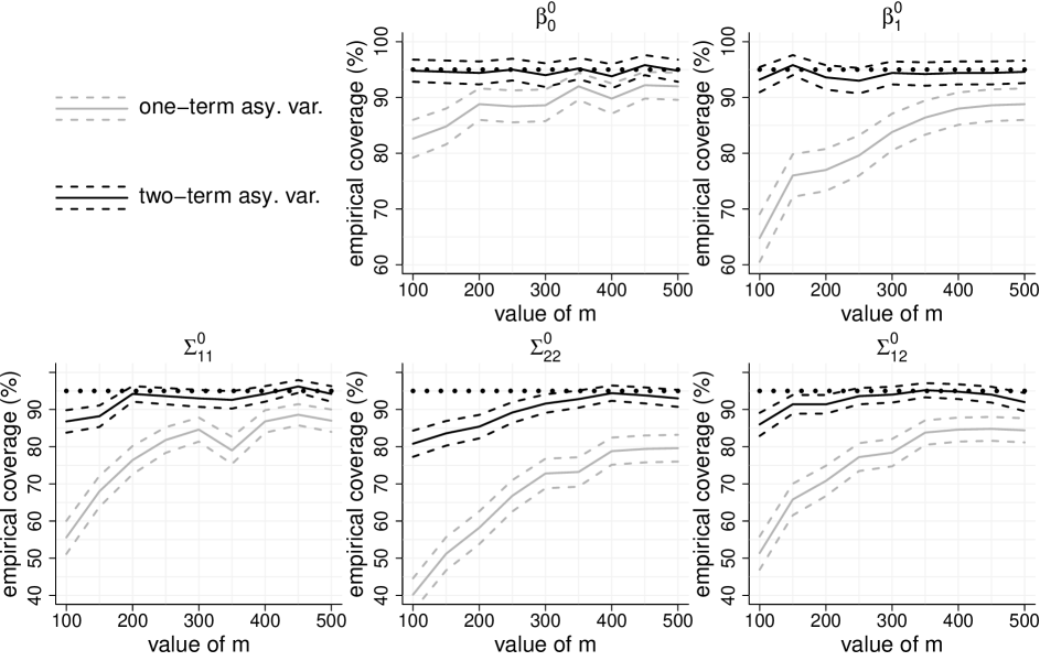
Figure 1: Empirical coverage of confidence intervals from the simulation exercise described in the text. Each panel corresponds to a model parameter that is impacted by second term asymptotic improvements. The advertised coverage level is fixed at 95% and is indicated by a horizontal dotted line in each panel. The solid curves show, dependent on the number of groups $m$, the empirical coverage levels for confidence intervals that use both one-term and two-term asymptotic variance approximations. The dashed curves correspond to plus and minus two standard errors of the sample proportions. The within-group sample size, $n$, is fixed at $m/10$.

Note that the confidence intervals for $\beta_{0}^{0}$, $\beta_{1}^{0}$ and the entries of $\boldsymbol{\Sigma}^{0}$ differ according to the two approaches since the estimators of these parameters have order $m^{-1}$ asymptotic variances. The confidence intervals for $\beta_{2}^{0}$, $\beta_{3}^{0}$ and $\beta_{4}^{0}$ are unaffected by the second term asymptotic improvements since their estimators have order $(mn)^{-1}$ asymptotic variances.

Figure 1 compares the empirical coverages of confidence intervals with advertised levels of 95% for the one-term asymptotic variances of Jiang et al. (2022) and the two-term asymptotic variances that arise from (9). In Figure 1 we only consider the parameters that are affected by second term improvement. The empirical coverages for the other parameters are provided in the supplement.

It is clear from Figure 1 that our second term improvements lead to much better coverages for lower sample size situations. On the other hand, one-term confidence intervals are trivial to compute whilst the two-term versions require considerable computing involving numerical integration.

Simulation results such as those summarised by Figure 1 provide an appreciation for the practical trade-offs arising from precise asymptotics for generalised linear mixed models.

References

Balasubramanian, N., Johnson, S.G., Hahn, T., Bouvier, A. & Kiêu, K. (2023). cubature 2.0.4.6: Adaptive multivariate integration over hypercubes. R package.
https://r-project.org

Bhaskaran, A. and Wand, M.P. (2023). Dispersion parameter extension of precise generalized linear mixed model asymptotics. Statistics and Probability Letters, 193, Article 109691.

Jiang, J. & Nguyen, T. (2021). Linear and Generalized Linear Mixed Models and Their Applications, Second Edition. New York: Springer.

Jiang, J., Wand, M.P. & Bhaskaran, A. (2022). Usable and precise asymptotics for generalized linear mixed model analysis and design. Journal of the Royal Statistical Society, Series B, 84, 55–82.

McCulloch, C.E., Searle, S.R. & Neuhaus, J.M. (2008). Generalized, Linear, and Mixed Models. Second Edition. New York: John Wiley & Sons.

Stroup, W.W. (2013). Generalized Linear Mixed Models. Boca Raton, Florida: CRC Press.

Supplement for:

Second Term Improvements to Generalised

Linear Mixed Model Asymptotics

By Luca Maestrini¹, Aishwarya Bhaskaran² and Matt P. Wand³

¹The Australian National University, ²Macquarie University and ³University of Technology Sydney

S.1 Introduction

The purpose of this supplement is to provide detailed derivational steps for the main result of Section 3.3 and further details on our simulation exercise. Sections S.2–S.5 provide relevant results concerning matrix algebra and multivariate calculus. In Sections S.6–S.9 we focus on the scores of the model parameters and their high-order asymptotic approximations. Sections S.10 and S.11 are concerned with approximation of the Fisher information matrix. The final stages of the derivations of (9) and (10) are given in Sections S.12 and S.14. Section S.15 provides some additional empirical coverage plots from the logistic mixed model simulation exercise described in Section 5.

S.2 Matrix Algebraic Results

The derivation of the results in Section 3.3 benefits from particular matrix results, which are summarized in this section.

For each $d\in{\mathbb{N}}$ the $d^{2}\times{\textstyle{\frac{1}{2}}}d(d+1)$ matrix $\boldsymbol{D}_{d}$ and $d^{2}\times d^{2}$ matrix $\boldsymbol{K}_{d}$ are constant matrices containing zeroes and ones such that

$$\boldsymbol{D}_{d}\mbox{\rm vech}(\boldsymbol{A})=\mbox{\rm vec}(\boldsymbol{A})\quad\mbox{for all symmetric $d\times d$ matrices $\boldsymbol{A}$}$$

and

$$\boldsymbol{K}_{d}\mbox{\rm vec}(\boldsymbol{B})=\mbox{\rm vec}(\boldsymbol{B}^{T})\quad\mbox{for all $d\times d$ matrices $\boldsymbol{B}$}.$$

Examples are

$$\boldsymbol{D}_{2}=\left[\begin{array}[]{ccc}1&0&0\\ 0&1&0\\ 0&1&0\\ 0&0&1\end{array}\right]\quad\mbox{and}\quad\boldsymbol{K}_{2}=\left[\begin{array}[]{cccc}1&0&0&0\\ 0&0&1&0\\ 0&1&0&0\\ 0&0&0&1\end{array}\right].$$

The $\boldsymbol{D}_{d}$ are called duplication matrices, whilst the $\boldsymbol{K}_{d}$ are called commutation matrices. As stated in Section 2, the Moore-Penrose inverse of $\boldsymbol{D}_{d}$ is $\boldsymbol{D}_{d}^{+}=(\boldsymbol{D}_{d}^{T}\boldsymbol{D}_{d})^{-1}\boldsymbol{D}_{d}^{T}$. Chapter 3 of Magnus & Neudecker (1999) contains several results concerning these families of matrices, a few of which are relevant to the derivation of (9). For convenience, we list them here.

Theorem 9(c) in Chapter 3 of Magnus & Neudecker (1999) implies that for any $d\times d$ matrix $\boldsymbol{A}$ and $d\times 1$ vector $\boldsymbol{b}$, we have

$$\boldsymbol{K}_{d}(\boldsymbol{A}\otimes\boldsymbol{b})=\boldsymbol{b}\otimes\boldsymbol{A}.$$ (S.1)

Theorem 12(a) in the same chapter asserts that

$$\boldsymbol{K}_{d}\boldsymbol{D}_{d}=\boldsymbol{D}_{d}$$ (S.2)

and implies that, for any $d\times d$ matrix $\boldsymbol{A}$,

$$\boldsymbol{D}_{d}^{T}\mbox{\rm vec}(\boldsymbol{A})=\boldsymbol{D}_{d}^{T}\mbox{\rm vec}(\boldsymbol{A}^{T}).$$ (S.3)

Also, Theorem 13(b) and Theorem 13(d) provide for a $d\times d$ matrix $\boldsymbol{A}$

$$\boldsymbol{D}_{d}\boldsymbol{D}_{d}^{+}(\boldsymbol{A}\otimes\boldsymbol{A})\boldsymbol{D}_{d}^{+T}=(\boldsymbol{A}\otimes\boldsymbol{A})\boldsymbol{D}_{d}^{+T}$$ (S.4)

and, assuming that $\boldsymbol{A}$ is invertible,

$$\big{\{}\boldsymbol{D}_{d}^{T}(\boldsymbol{A}\otimes\boldsymbol{A})\boldsymbol{D}_{d}\big{\}}^{-1}=\boldsymbol{D}_{d}^{+}(\boldsymbol{A}^{-1}\otimes\boldsymbol{A}^{-1})\boldsymbol{D}_{d}^{+T}.$$ (S.5)

Lastly, we state two matrix identities that are used in the derivations. For matrices $\boldsymbol{A}$, $\boldsymbol{B}$ and $\boldsymbol{C}$ such that $\boldsymbol{A}\boldsymbol{B}\boldsymbol{C}$ is defined, we have

$$\mbox{\rm vec}(\boldsymbol{A}\boldsymbol{B}\boldsymbol{C})=(\boldsymbol{C}^{T}\otimes\boldsymbol{A})\mbox{\rm vec}(\boldsymbol{B}).$$ (S.6)

For conformable matrices $\boldsymbol{A}$, $\boldsymbol{B}$, $\boldsymbol{C}$ and $\boldsymbol{D}$, we have

$${\color[rgb]{0,0,0}(\boldsymbol{A}\otimes\boldsymbol{B})(\boldsymbol{C}\otimes\boldsymbol{D})=(\boldsymbol{A}\boldsymbol{C})\otimes(\boldsymbol{B}\boldsymbol{D}).}$$ (S.7)

S.3 Multivariate Derivative Notation

For $f$ a smooth real-valued function of the $d$-variate argument $\boldsymbol{x}\equiv(x_{1},\ldots,x_{d})$, let $\nabla f(\boldsymbol{x})$ denote the $d\times 1$ vector with $r$th entry $\partial f(\boldsymbol{x})/\partial x_{r}$, $\nabla^{2}f(\boldsymbol{x})$ denote the $d\times d$ matrix with $(r,s)$ entry $\partial^{2}f(\boldsymbol{x})/(\partial x_{r}\partial x_{s})$ and $\nabla^{3}f(\boldsymbol{x})$ denote the $d\times d\times d$ array with $(r,s,t)$ entry $\partial^{3}f(\boldsymbol{x})/(\partial x_{r}\partial x_{s}\partial x_{t})$.

S.4 Three-Term Taylor Series Expansion of Gradient Vectors

Consider $f:{\mathbb{R}}^{d}\to{\mathbb{R}}$. Then, for sufficiently smooth $f$, the three-term Taylor expansion of

$$f(\boldsymbol{x}+\boldsymbol{h})\quad\mbox{where $\boldsymbol{x}\equiv(x_{1},\ldots,x_{d})$ and $\boldsymbol{h}\equiv(h_{1},\ldots,h_{d})$}$$

is

$$f(\boldsymbol{x}+\boldsymbol{h})=f(\boldsymbol{x})+\sum_{r=1}^{d}\{\nabla f(\boldsymbol{x})\}_{r}h_{r}+{\textstyle{\frac{1}{2}}}\sum_{r=1}^{d}\sum_{s=1}^{d}\{\nabla^{2}f(\boldsymbol{x})\}_{rs}h_{r}h_{s}+\ldots{\color[rgb]{0,0,0}.}$$ (S.8)

Now consider $\alpha:{\mathbb{R}}^{d}\to{\mathbb{R}}$ and its gradient function $\nabla\alpha:{\mathbb{R}}^{d}\to{\mathbb{R}}^{d}$. If (S.8) is applied to each entry of $(\nabla\alpha)(\boldsymbol{x}+\boldsymbol{h})$ then we have

$$\left[{\begin{array}[]{c}\{(\nabla\alpha)(\boldsymbol{x}+\boldsymbol{h})\}_{1}\\ \vdots\\ \{(\nabla\alpha)(\boldsymbol{x}+\boldsymbol{h})\}_{d}\end{array}}\right]=\left[{\begin{array}[]{c}\{(\nabla\alpha)(\boldsymbol{x})\}_{1}+{\displaystyle\sum_{r=1}^{d}}\{\nabla^{2}\alpha(\boldsymbol{x})\}_{r1}h_{r}+{\textstyle{\frac{1}{2}}}{\displaystyle\sum_{r=1}^{d}\sum_{s=1}^{d}}\{\nabla^{3}\alpha(\boldsymbol{x})\}_{rs1}h_{r}h_{s}\\ \vdots\\ \{(\nabla\alpha)(\boldsymbol{x})\}_{{\color[rgb]{0,0,0}d}}+{\displaystyle\sum_{r=1}^{d}}\{\nabla^{2}\alpha(\boldsymbol{x})\}_{r{\color[rgb]{0,0,0}d}}h_{r}+{\textstyle{\frac{1}{2}}}{\displaystyle\sum_{r=1}^{d}\sum_{s=1}^{d}}\{\nabla^{3}\alpha(\boldsymbol{x})\}_{rsd}h_{r}h_{s}\end{array}}\right]+\ldots.$$

From this it is clear that

$$(\nabla\alpha)(\boldsymbol{x}+\boldsymbol{h})=(\nabla\alpha)(\boldsymbol{x})+\{(\nabla^{2}\alpha)(\boldsymbol{x})\}\boldsymbol{h}+{\textstyle{\frac{1}{2}}}\{(\nabla^{3}\alpha)(\boldsymbol{x})\}\bigstar(\boldsymbol{h}\boldsymbol{h}^{T})+\ldots.$$ (S.9)

where the $\bigstar$ notation is as defined by (7).

S.5 Higher Order Approximation of Multivariate Integral Ratios

The main tool for approximation of the Fisher information matrix of (2) is higher order Laplace-type approximation of multivariate integral ratios. Appendix A of Miyata (2004) provides such a result, which states that for smooth real-valued $d$-variate functions $g$, $c$ and $h$,

$${\begin{array}[]{rcl}&&{\displaystyle\frac{\int_{{\mathbb{R}}^{d}}g(\boldsymbol{x})c(\boldsymbol{x})\exp\{-nh(\boldsymbol{x})\}\,d\boldsymbol{x}}{\int_{{\mathbb{R}}^{d}}c(\boldsymbol{x})\exp\{-nh(\boldsymbol{x})\}\,d\boldsymbol{x}}}=g(\boldsymbol{x}^{*})+{\displaystyle\frac{\nabla g(\boldsymbol{x}^{*})^{T}\{\nabla^{2}h(\boldsymbol{x}^{*})\}^{-1}\nabla c(\boldsymbol{x}^{*})}{nc(\boldsymbol{x}^{*})}}\\[12.91663pt] &&\qquad+{\displaystyle\frac{\mbox{tr}[\{\nabla^{2}h(\boldsymbol{x}^{*})\}^{-1}\nabla^{2}g(\boldsymbol{x}^{*})]}{2n}}-{\displaystyle\frac{\nabla g(\boldsymbol{x}^{*})^{T}\{\nabla^{2}h(\boldsymbol{x}^{*})\}^{-1}\Big{[}\nabla^{3}h(\boldsymbol{x}^{*})\bigstar\{\nabla^{2}h(\boldsymbol{x}^{*})\}^{-1}\Big{]}}{2n}}+O(n^{-2})\end{array}}$$ (S.10)

where

$$\boldsymbol{x}^{*}\equiv\mathop{\mbox{\rm argmin}}_{\boldsymbol{x}\in{\mathbb{R}}^{d}}h(\boldsymbol{x}).$$

S.6 Exact Score Expressions

For $1\leq i\leq m$, let $p_{\mbox{\tiny$\boldsymbol{Y}_{i}|\boldsymbol{X}_{i}$}}$ denote the conditional density function, or probability mass function, of $\boldsymbol{Y}_{i}$ given $\boldsymbol{X}_{i}$. Then let

$$\boldsymbol{S}_{\mbox{\scriptsize A}i}\equiv\nabla_{\mbox{\tiny$\boldsymbol{\beta}_{\mbox{\tiny A}}$}}\log p_{\mbox{\tiny$\boldsymbol{Y}_{i}|\boldsymbol{X}_{i}$}}(\boldsymbol{Y}_{i}|\boldsymbol{X}_{i}),\quad\boldsymbol{S}_{\mbox{\scriptsize B}i}\equiv\nabla_{\mbox{\tiny$\boldsymbol{\beta}_{\mbox{\tiny B}}$}}\log p_{\mbox{\tiny$\boldsymbol{Y}_{i}|\boldsymbol{X}_{i}$}}(\boldsymbol{Y}_{i}|\boldsymbol{X}_{i})$$

and

$$\boldsymbol{S}_{\mbox{\scriptsize C}i}\equiv\nabla_{\mbox{\scriptsize$\mbox{\rm vech}(\boldsymbol{\Sigma})$}}\log p_{\mbox{\tiny$\boldsymbol{Y}_{i}|\boldsymbol{X}_{i}$}}(\boldsymbol{Y}_{i}|\boldsymbol{X}_{i})$$

denote the $i$th contribution to the scores with respect to each of $\boldsymbol{\beta}_{\mbox{\scriptsize A}}$, $\boldsymbol{\beta}_{\mbox{\scriptsize B}}$ and $\mbox{\rm vech}(\boldsymbol{\Sigma})$. Then it is straightforward to show that the exact scores are

$$\boldsymbol{S}_{\mbox{\scriptsize A}i}=\frac{\int_{{\mathbb{R}}^{d_{\mbox{\tiny R}}}}\boldsymbol{g}_{\scriptscriptstyle iA}(\boldsymbol{u})c_{\scriptscriptstyle S}(\boldsymbol{u})\exp\{-nh_{i}(\boldsymbol{u})\}\,d\boldsymbol{u}}{\int_{{\mathbb{R}}^{d_{\mbox{\tiny R}}}}c_{\scriptscriptstyle S}(\boldsymbol{u})\exp\{-nh_{i}(\boldsymbol{u})\}\,d\boldsymbol{u}},$$ (S.11)

$$\boldsymbol{S}_{\mbox{\scriptsize B}i}=\frac{\int_{{\mathbb{R}}^{d_{\mbox{\tiny R}}}}\boldsymbol{g}_{\scriptscriptstyle iB}(\boldsymbol{u})c_{\scriptscriptstyle S}(\boldsymbol{u})\exp\{-nh_{i}(\boldsymbol{u})\}\,d\boldsymbol{u}}{\int_{{\mathbb{R}}^{d_{\mbox{\tiny R}}}}c_{\scriptscriptstyle S}(\boldsymbol{u})\exp\{-nh_{i}(\boldsymbol{u})\}\,d\boldsymbol{u}}$$ (S.12)

and

$$\boldsymbol{S}_{\mbox{\scriptsize C}i}=\frac{\int_{{\mathbb{R}}^{d_{\mbox{\tiny R}}}}\boldsymbol{g}_{\scriptscriptstyle iC}(\boldsymbol{u})c_{\scriptscriptstyle S}(\boldsymbol{u})\exp\{-nh_{i}(\boldsymbol{u})\}\,d\boldsymbol{u}}{\int_{{\mathbb{R}}^{d_{\mbox{\tiny R}}}}c_{\scriptscriptstyle S}(\boldsymbol{u})\exp\{-nh_{i}(\boldsymbol{u})\}\,d\boldsymbol{u}}-{\textstyle{\frac{1}{2}}}\boldsymbol{D}_{d_{\mbox{\tiny R}}}^{T}\mbox{\rm vec}(\boldsymbol{\Sigma}^{-1})$$ (S.13)

where

$$c_{\scriptscriptstyle S}(\boldsymbol{u}) \equiv \exp(-{\textstyle{\frac{1}{2}}}\boldsymbol{u}^{T}\boldsymbol{\Sigma}^{-1}\boldsymbol{u}),\quad\boldsymbol{g}_{\scriptscriptstyle iA}(\boldsymbol{u})\equiv\boldsymbol{\Sigma}^{-1}\boldsymbol{u},$$

$$\boldsymbol{g}_{\scriptscriptstyle iB}(\boldsymbol{u}) \equiv \frac{1}{\phi}{\displaystyle\sum_{j=1}^{n_{i}}}\boldsymbol{X}_{\mbox{\scriptsize B}ij}\{Y_{ij}-b^{\prime}\big{(}(\boldsymbol{\beta}_{\mbox{\scriptsize A}}+\boldsymbol{u})^{T}\boldsymbol{X}_{\mbox{\scriptsize A}ij}+\boldsymbol{\beta}_{\mbox{\scriptsize B}}^{T}\boldsymbol{X}_{\mbox{\scriptsize B}ij}\big{)}\},$$

$$\boldsymbol{g}_{\scriptscriptstyle iC}(\boldsymbol{u}) \equiv {\textstyle{\frac{1}{2}}}\boldsymbol{D}_{d_{\mbox{\tiny R}}}^{T}(\boldsymbol{\Sigma}^{-1}\otimes\boldsymbol{\Sigma}^{-1})\mbox{\rm vec}(\boldsymbol{u}\boldsymbol{u}^{T})$$

$$\mbox{and}\quad h_{i}(\boldsymbol{u}) \equiv \,-\frac{1}{n\phi}{\displaystyle\sum_{j=1}^{n_{i}}}\left\{Y_{ij}\boldsymbol{u}^{T}\boldsymbol{X}_{\mbox{\scriptsize A}ij}-b\big{(}(\boldsymbol{\beta}_{\mbox{\scriptsize A}}+\boldsymbol{u})^{T}\boldsymbol{X}_{\mbox{\scriptsize A}ij}+\boldsymbol{\beta}_{\mbox{\scriptsize B}}^{T}\boldsymbol{X}_{\mbox{\scriptsize B}ij}\big{)}\right\}.$$

An integration by parts step is used to obtain the $\boldsymbol{S}_{\mbox{\scriptsize A}i}$ expression.

In the upcoming sections we obtain asymptotic approximations of $\boldsymbol{S}_{\mbox{\scriptsize A}i}$ $\boldsymbol{S}_{\mbox{\scriptsize B}i}$ and $\boldsymbol{S}_{\mbox{\scriptsize C}i}$. Key quantities for these approximations are

$$\boldsymbol{U}_{i}^{*}\equiv\mathop{\mbox{\rm argmin}}_{\boldsymbol{u}\in{\mathbb{R}}^{d_{\mbox{\tiny R}}}}h_{i}(\boldsymbol{u}),\quad 1\leq i\leq m.$$

S.7 Definitions of Key Summation Quantities

Our derivation of (9) involves manipulations of particular summation quantities, which are defined in this section. At the end of this section we state some important moment-type relationships between the quantities.

For each $1\leq i\leq m$, define ${\mathcal{G}}_{\mbox{\scriptsize A}i}$, ${\mathcal{G}}_{\mbox{\scriptsize B}i}$, ${\mathcal{H}}_{\mbox{\scriptsize AA}i}$, ${\mathcal{H}}_{\mbox{\scriptsize AB}i}$, and ${\mathcal{H}}_{\mbox{\scriptsize BB}i}$ as follows:

$${\mathcal{G}}_{\mbox{\scriptsize A}i} \equiv {\displaystyle\sum_{j=1}^{n_{i}}}\{Y_{ij}-b^{\prime}\big{(}(\boldsymbol{\beta}_{\mbox{\scriptsize A}}+\boldsymbol{U}_{i})^{T}\boldsymbol{X}_{\mbox{\scriptsize A}ij}+\boldsymbol{\beta}_{\mbox{\scriptsize B}}^{T}\boldsymbol{X}_{\mbox{\scriptsize B}ij}\big{)}\}\boldsymbol{X}_{\mbox{\scriptsize A}ij},$$

$${\mathcal{G}}_{\mbox{\scriptsize B}i} \equiv {\displaystyle\sum_{j=1}^{n_{i}}}\{Y_{ij}-b^{\prime}\big{(}(\boldsymbol{\beta}_{\mbox{\scriptsize A}}+\boldsymbol{U}_{i})^{T}\boldsymbol{X}_{\mbox{\scriptsize A}ij}+\boldsymbol{\beta}_{\mbox{\scriptsize B}}^{T}\boldsymbol{X}_{\mbox{\scriptsize B}ij}\big{)}\}\boldsymbol{X}_{\mbox{\scriptsize B}ij},$$

$${\mathcal{H}}_{\mbox{\scriptsize AA}i} \equiv {\displaystyle\sum_{j=1}^{n_{i}}}b^{\prime\prime}\big{(}(\boldsymbol{\beta}_{\mbox{\scriptsize A}}+\boldsymbol{U}_{i})^{T}\boldsymbol{X}_{\mbox{\scriptsize A}ij}+\boldsymbol{\beta}_{\mbox{\scriptsize B}}^{T}\boldsymbol{X}_{\mbox{\scriptsize B}ij}\big{)}\boldsymbol{X}_{\mbox{\scriptsize A}ij}\boldsymbol{X}_{\mbox{\scriptsize A}ij}^{T},$$

$${\mathcal{H}}_{\mbox{\scriptsize AB}i} \equiv {\displaystyle\sum_{j=1}^{n_{i}}}b^{\prime\prime}\big{(}(\boldsymbol{\beta}_{\mbox{\scriptsize A}}+\boldsymbol{U}_{i})^{T}\boldsymbol{X}_{\mbox{\scriptsize A}ij}+\boldsymbol{\beta}_{\mbox{\scriptsize B}}^{T}\boldsymbol{X}_{\mbox{\scriptsize B}ij}\big{)}\boldsymbol{X}_{\mbox{\scriptsize A}ij}\boldsymbol{X}_{\mbox{\scriptsize B}ij}^{T}$$

$$\mbox{and}\quad{\mathcal{H}}_{\mbox{\scriptsize BB}i} \equiv {\displaystyle\sum_{j=1}^{n_{i}}}b^{\prime\prime}\big{(}(\boldsymbol{\beta}_{\mbox{\scriptsize A}}+\boldsymbol{U}_{i})^{T}\boldsymbol{X}_{\mbox{\scriptsize A}ij}+\boldsymbol{\beta}_{\mbox{\scriptsize B}}^{T}\boldsymbol{X}_{\mbox{\scriptsize B}ij}\big{)}\boldsymbol{X}_{\mbox{\scriptsize B}ij}\boldsymbol{X}_{\mbox{\scriptsize B}ij}^{T}.$$

In a similar vein, define ${\mathcal{H}}^{\prime}_{\mbox{\scriptsize AAA}i}$ to be the $d_{\mbox{\tiny R}}\times d_{\mbox{\tiny R}}\times d_{\mbox{\tiny R}}$ array with $(r,s,t)$ entry equal to

$${\displaystyle\sum_{j=1}^{n_{i}}}b^{\prime\prime\prime}\big{(}(\boldsymbol{\beta}_{\mbox{\scriptsize A}}+\boldsymbol{U}_{i})^{T}\boldsymbol{X}_{\mbox{\scriptsize A}ij}+\boldsymbol{\beta}_{\mbox{\scriptsize B}}^{T}\boldsymbol{X}_{\mbox{\scriptsize B}ij}\big{)}(\boldsymbol{X}_{\mbox{\scriptsize A}ij})_{r}(\boldsymbol{X}_{\mbox{\scriptsize A}ij})_{s}(\boldsymbol{X}_{\mbox{\scriptsize A}ij})_{t}$$

and ${\mathcal{H}}^{\prime}_{\mbox{\scriptsize AAB}i}$ to be the $d_{\mbox{\tiny R}}\times d_{\mbox{\tiny R}}\times d_{\mbox{\tiny B}}$ array with $(r,s,t)$ entry equal to

$${\displaystyle\sum_{j=1}^{n_{i}}}b^{\prime\prime\prime}\big{(}(\boldsymbol{\beta}_{\mbox{\scriptsize A}}+\boldsymbol{U}_{i})^{T}\boldsymbol{X}_{\mbox{\scriptsize A}ij}+\boldsymbol{\beta}_{\mbox{\scriptsize B}}^{T}\boldsymbol{X}_{\mbox{\scriptsize B}ij}\big{)}(\boldsymbol{X}_{\mbox{\scriptsize A}ij})_{r}(\boldsymbol{X}_{\mbox{\scriptsize A}ij})_{s}(\boldsymbol{X}_{\mbox{\scriptsize B}ij})_{t}$$

where

$$d_{\mbox{\tiny B}}\equiv d_{\mbox{\tiny F}}-d_{\mbox{\tiny R}}.$$

The following relationships are of fundamental importance for the derivation of (9):

$$\begin{array}[]{c}E\big{(}{\mathcal{G}}_{\mbox{\scriptsize A}i}|\boldsymbol{X}_{i},\boldsymbol{U}_{i}\big{)}=\boldsymbol{0},\quad E\big{(}{\mathcal{G}}_{\mbox{\scriptsize B}i}|\boldsymbol{X}_{i},\boldsymbol{U}_{i}\big{)}=\boldsymbol{0},\\[4.30554pt] E\big{(}{\mathcal{G}}_{\mbox{\scriptsize A}i}^{\otimes 2}|\boldsymbol{X}_{i},\boldsymbol{U}_{i}\big{)}=\phi{\mathcal{H}}_{\mbox{\scriptsize AA}i},\quad E\big{(}{\mathcal{G}}_{\mbox{\scriptsize A}i}{\mathcal{G}}_{\mbox{\scriptsize B}i}^{T}|\boldsymbol{X}_{i},\boldsymbol{U}_{i}\big{)}=\phi{\mathcal{H}}_{\mbox{\scriptsize AB}i}{\color[rgb]{0,0,0}\quad\mbox{and}\quad E\big{(}{\mathcal{G}}_{\mbox{\scriptsize B}i}^{\otimes 2}|\boldsymbol{X}_{i},\boldsymbol{U}_{i}\big{)}=\phi{\mathcal{H}}_{\mbox{\scriptsize BB}i}}\end{array}$$ (S.14)

where, throughout this supplement,

$$\boldsymbol{v}^{\otimes 2}\equiv\boldsymbol{v}\boldsymbol{v}^{T}\quad\mbox{for any column vector $\boldsymbol{v}$}.$$

Also note that

$${\mathcal{G}}_{\mbox{\scriptsize A}i}=O_{p}(n^{1/2})\boldsymbol{1}_{d_{\mbox{\tiny R}}},\quad{\mathcal{G}}_{\mbox{\scriptsize B}i}=O_{p}(n^{1/2})\boldsymbol{1}_{d_{\mbox{\tiny B}}},\quad{\mathcal{H}}_{\mbox{\scriptsize AA}i}=O_{p}(n)\boldsymbol{1}_{d_{\mbox{\tiny R}}}^{\otimes 2},$$

$${\mathcal{H}}_{\mbox{\scriptsize BB}i}=O_{p}(n)\boldsymbol{1}_{d_{\mbox{\tiny B}}}^{\otimes 2},\quad{\mathcal{H}}_{\mbox{\scriptsize AB}i}=O_{p}(n)\boldsymbol{1}_{d_{\mbox{\tiny R}}}\boldsymbol{1}_{d_{\mbox{\tiny B}}}^{T}$$

and that all entries of ${\mathcal{H}}^{\prime}_{\mbox{\scriptsize AAA}i}$ and ${\mathcal{H}}^{\prime}_{\mbox{\scriptsize AAB}i}$ are $O_{p}(n)$.

S.8 Approximation of $\boldsymbol{U}_{i}^{*}$

Use of (S.10) to approximate $\boldsymbol{S}_{\mbox{\scriptsize A}i}$, $\boldsymbol{S}_{\mbox{\scriptsize B}i}$ and $\boldsymbol{S}_{\mbox{\scriptsize C}i}$ requires approximation of $\boldsymbol{U}_{i}^{*}$. Introduce the notation ${\mathcal{C}}_{i}(\boldsymbol{u})\equiv n\phi h_{i}(\boldsymbol{u})$. Then $\boldsymbol{U}_{i}^{*}$ satisfies

$$\nabla{\mathcal{C}}_{i}(\boldsymbol{U}_{i}^{*})=\boldsymbol{0}$$

where

$$\nabla{\mathcal{C}}_{i}(\boldsymbol{u})\equiv-{\displaystyle\sum_{j=1}^{n_{i}}}\Big{\{}Y_{ij}-b^{\prime}\big{(}(\boldsymbol{\beta}_{\mbox{\scriptsize A}}+\boldsymbol{u})^{T}\boldsymbol{X}_{\mbox{\scriptsize A}ij}+\boldsymbol{\beta}_{\mbox{\scriptsize B}}^{T}\boldsymbol{X}_{\mbox{\scriptsize B}ij}\big{)}\Big{\}}\boldsymbol{X}_{\mbox{\scriptsize A}ij}.$$

Then, from (S.9) we have

$$\nabla{\mathcal{C}}_{i}(\boldsymbol{U}_{i}^{*}) = \nabla{\mathcal{C}}_{i}(\boldsymbol{U}_{i}+\boldsymbol{U}_{i}^{*}-\boldsymbol{U}_{i})$$

$$= \nabla{\mathcal{C}}_{i}(\boldsymbol{U}_{i})+\{\nabla^{2}{\mathcal{C}}_{i}(\boldsymbol{U}_{i})\}(\boldsymbol{U}_{i}^{*}-\boldsymbol{U}_{i})$$

$$\qquad+{\textstyle{\frac{1}{2}}}\left\{\nabla^{3}{\mathcal{C}}_{i}(\boldsymbol{U}_{i})\right\}\bigstar\{(\boldsymbol{U}_{i}^{*}-\boldsymbol{U}_{i})(\boldsymbol{U}_{i}^{*}-\boldsymbol{U}_{i})^{T}\}+\ldots.$$

Next we seek explicit expressions for $\nabla^{2}{\mathcal{C}}_{i}(\boldsymbol{u})$ and $\nabla^{3}{\mathcal{C}}_{i}(\boldsymbol{u})$. Standard vector calculus arguments lead to

$$\nabla^{2}{\mathcal{C}}_{i}(\boldsymbol{u}) = {\displaystyle\sum_{j=1}^{n_{i}}}b^{\prime\prime}\big{(}(\boldsymbol{\beta}_{\mbox{\scriptsize A}}+\boldsymbol{u})^{T}\boldsymbol{X}_{\mbox{\scriptsize A}ij}+\boldsymbol{\beta}_{\mbox{\scriptsize B}}^{T}\boldsymbol{X}_{\mbox{\scriptsize B}ij}\big{)}\boldsymbol{X}_{\mbox{\scriptsize A}ij}\boldsymbol{X}_{\mbox{\scriptsize A}ij}^{T}$$

$$= \left[{\displaystyle\sum_{j=1}^{n_{i}}}b^{\prime\prime}\big{(}(\boldsymbol{\beta}_{\mbox{\scriptsize A}}+\boldsymbol{u})^{T}\boldsymbol{X}_{\mbox{\scriptsize A}ij}+\boldsymbol{\beta}_{\mbox{\scriptsize B}}^{T}\boldsymbol{X}_{\mbox{\scriptsize B}ij}\big{)}(\boldsymbol{X}_{\mbox{\scriptsize A}ij})_{r}(\boldsymbol{X}_{\mbox{\scriptsize A}ij})_{s}\right]_{1\leq r,s\leq d_{\mbox{\tiny R}}}.$$

Then, the three-dimension array of all third order partial derivatives of ${\mathcal{C}}_{i}(u)$ is

$$\nabla^{3}{\mathcal{C}}_{i}(\boldsymbol{u})=\left[{\displaystyle\sum_{j=1}^{n_{i}}}b^{\prime\prime\prime}\big{(}(\boldsymbol{\beta}_{\mbox{\scriptsize A}}+\boldsymbol{u})^{T}\boldsymbol{X}_{\mbox{\scriptsize A}ij}+\boldsymbol{\beta}_{\mbox{\scriptsize B}}^{T}\boldsymbol{X}_{\mbox{\scriptsize B}ij}\big{)}(\boldsymbol{X}_{\mbox{\scriptsize A}ij})_{r}(\boldsymbol{X}_{\mbox{\scriptsize A}ij})_{s}(\boldsymbol{X}_{\mbox{\scriptsize A}ij})_{t}\right]_{1\leq r,s,t\leq d_{\mbox{\tiny R}}}.$$

We then have

$$\nabla{\mathcal{C}}_{i}(\boldsymbol{U}_{i}^{*})=-{\mathcal{G}}_{\mbox{\scriptsize A}i}+{\mathcal{H}}_{\mbox{\scriptsize AA}i}(\boldsymbol{U}_{i}^{*}-\boldsymbol{U}_{i})+{\textstyle{\frac{1}{2}}}{\mathcal{H}}^{\prime}_{\mbox{\scriptsize AAA}i}\bigstar\{(\boldsymbol{U}_{i}^{*}-\boldsymbol{U}_{i})(\boldsymbol{U}_{i}^{*}-\boldsymbol{U}_{i})^{T}\}+\ldots$$

and so $\nabla{\mathcal{C}}_{i}(\boldsymbol{U}_{i}^{*})=\boldsymbol{0}$ is equivalent to

$${\mathcal{H}}_{\mbox{\scriptsize AA}i}^{-1}{\mathcal{G}}_{\mbox{\scriptsize A}i}=(\boldsymbol{U}_{i}^{*}-\boldsymbol{U}_{i})+{\textstyle{\frac{1}{2}}}{\mathcal{H}}_{\mbox{\scriptsize AA}i}^{-1}{\color[rgb]{0,0,0}\Big{[}}{\mathcal{H}}^{\prime}_{\mbox{\scriptsize AAA}i}\bigstar\{(\boldsymbol{U}_{i}^{*}-\boldsymbol{U}_{i})(\boldsymbol{U}_{i}^{*}-\boldsymbol{U}_{i})^{T}\}{\color[rgb]{0,0,0}\Big{]}}+\ldots.$$ (S.15)

We now invert (S.15) using the set-up given around equations (9.43) and (9.44) of Pace & Salvan (1997). To match the notation given there, set

$$\boldsymbol{y}\equiv{\mathcal{H}}_{\mbox{\scriptsize AA}i}^{-1}{\mathcal{G}}_{\mbox{\scriptsize A}i}\quad\mbox{and}\quad\boldsymbol{x}\equiv\boldsymbol{U}_{i}^{*}-\boldsymbol{U}_{i}.$$

Then, in keeping with the displayed equation just before (9.43) of Pace & Salvan (1997) and using their superscript and subscript conventions, we have

$$y^{a}\equiv\mbox{the $a$th entry of $\boldsymbol{y}$}\quad\mbox{and}\quad x^{a}\equiv\mbox{the $a$th entry of $\boldsymbol{x}$}.$$

Also,

$$x^{rs}\equiv x^{r}x^{s}=\mbox{the $(r,s)$ entry of $\boldsymbol{x}\boldsymbol{x}^{T}$}=\mbox{the $(r,s)$ entry of $(\boldsymbol{U}_{i}^{*}-\boldsymbol{U}_{i})^{\otimes 2}$}.$$

Then

$$y^{a}=x^{a}+A_{rs}^{a}x^{rs}+\ldots.$$

where

$$A_{rs}^{a}\boldsymbol{x}^{rs} = \mbox{the $a$th entry of}\ {\textstyle{\frac{1}{2}}}{\mathcal{H}}_{\mbox{\scriptsize AA}i}^{-1}{\color[rgb]{0,0,0}\Big{[}}{\mathcal{H}}^{\prime}_{\mbox{\scriptsize AAA}i}\bigstar\{(\boldsymbol{U}_{i}^{*}-\boldsymbol{U}_{i})(\boldsymbol{U}_{i}^{*}-\boldsymbol{U}_{i})^{T}\}{\color[rgb]{0,0,0}\Big{]}}$$

$$= \mbox{the $a$th entry of}\ {\textstyle{\frac{1}{2}}}{\mathcal{H}}_{\mbox{\scriptsize AA}i}^{-1}{\color[rgb]{0,0,0}\Big{\{}}{\mathcal{H}}^{\prime}_{\mbox{\scriptsize AAA}i}\bigstar(\boldsymbol{x}\boldsymbol{x}^{T}){\color[rgb]{0,0,0}\Big{\}}}.$$

From equations (9.43) and (9.44) of Pace & Salvan (1997),

$$x^{a} = y^{a}-A_{rs}^{a}y^{rs}+\ldots$$

$$= y^{a}-\mbox{the $a$th entry of}\ {\textstyle{\frac{1}{2}}}{\mathcal{H}}_{\mbox{\scriptsize AA}i}^{-1}{\color[rgb]{0,0,0}\Big{\{}}{\mathcal{H}}^{\prime}_{\mbox{\scriptsize AAA}i}\bigstar(\boldsymbol{y}\boldsymbol{y}^{T}){\color[rgb]{0,0,0}\Big{\}}}+\ldots$$

$$= y^{a}-\mbox{the $a$th entry of}\ {\textstyle{\frac{1}{2}}}{\mathcal{H}}_{\mbox{\scriptsize AA}i}^{-1}{\color[rgb]{0,0,0}\Big{\{}}{\mathcal{H}}^{\prime}_{\mbox{\scriptsize AAA}i}\bigstar{\color[rgb]{0,0,0}\Big{(}}{\mathcal{H}}_{\mbox{\scriptsize AA}i}^{-1}{\mathcal{G}}_{\mbox{\scriptsize A}i}{\color[rgb]{0,0,0}\Big{)}}^{\otimes 2}{\color[rgb]{0,0,0}\Big{\}}}+\ldots.$$

This results in the following three-term approximation of $\boldsymbol{U}_{i}^{*}$:

$$\boldsymbol{U}_{i}^{*}=\boldsymbol{U}_{i}+{\mathcal{H}}_{\mbox{\scriptsize AA}i}^{-1}{\mathcal{G}}_{\mbox{\scriptsize A}i}-{\textstyle{\frac{1}{2}}}{\mathcal{H}}_{\mbox{\scriptsize AA}i}^{-1}\Big{\{}{\mathcal{H}}^{\prime}_{\mbox{\scriptsize AAA}i}\bigstar{\color[rgb]{0,0,0}\Big{(}}{\mathcal{H}}_{\mbox{\scriptsize AA}i}^{-1}{\mathcal{G}}_{\mbox{\scriptsize A}i}{\mathcal{G}}_{\mbox{\scriptsize A}i}^{T}{\mathcal{H}}_{\mbox{\scriptsize AA}i}^{-1}{\color[rgb]{0,0,0}\Big{)}}\Big{\}}+O_{p}(n^{-3/2})\boldsymbol{1}_{d_{\mbox{\tiny R}}}.$$ (S.16)

S.9 Score Asymptotic Approximation

We are now ready to obtain approximations of the scores $\boldsymbol{S}_{\mbox{\scriptsize A}i}$, $\boldsymbol{S}_{\mbox{\scriptsize B}i}$ and $\boldsymbol{S}_{\mbox{\scriptsize C}i}$ with accuracies that are sufficient for the two-term asymptotic covariance matrices of (9).

S.9.1 Approximation of $\boldsymbol{S}_{\mbox{\scriptsize A}i}$

For each $1\leq r\leq d_{\mbox{\tiny R}}$, let $\boldsymbol{e}_{r}$ denote the $d_{\mbox{\tiny R}}\times 1$ vector having $r$th entry equal to 1 and zeroes elsewhere.

S.9.1.1 The (S.10) First Term Contribution

For each $1\leq r\leq d_{\mbox{\tiny R}}$, the contribution to the $r$th entry of $\boldsymbol{S}_{\mbox{\scriptsize A}i}$ from the first term on the right-hand side of (S.10) is $\mbox{the $r$th entry of}\ \boldsymbol{\Sigma}^{-1}\boldsymbol{U}_{i}^{*}.$ In view of (S.16) we obtain the following contribution to $\boldsymbol{S}_{\mbox{\scriptsize A}i}$:

$$\boldsymbol{\Sigma}^{-1}\boldsymbol{U}_{i}+\boldsymbol{\Sigma}^{-1}{\mathcal{H}}_{\mbox{\scriptsize AA}i}^{-1}{\mathcal{G}}_{\mbox{\scriptsize A}i}-{\textstyle{\frac{1}{2}}}\boldsymbol{\Sigma}^{-1}{\mathcal{H}}_{\mbox{\scriptsize AA}i}^{-1}\Big{\{}{\mathcal{H}}^{\prime}_{\mbox{\scriptsize AAA}i}\bigstar\Big{(}{\mathcal{H}}_{\mbox{\scriptsize AA}i}^{-1}{\mathcal{G}}_{\mbox{\scriptsize A}i}{\mathcal{G}}_{\mbox{\scriptsize A}i}^{T}{\mathcal{H}}_{\mbox{\scriptsize AA}i}^{-1}\Big{)}\Big{\}}+O_{p}(n^{-3/2})\boldsymbol{1}_{d_{\mbox{\tiny R}}}.$$

S.9.1.2 The (S.10) Second Term Contribution

Noting that

$$\nabla\{\boldsymbol{e}_{r}^{T}\boldsymbol{g}_{\scriptscriptstyle iA}(\boldsymbol{u})\}=\boldsymbol{e}_{r}^{T}\boldsymbol{\Sigma}^{-1}\quad\mbox{and}\quad\nabla c_{\scriptscriptstyle S}(\boldsymbol{u})=-c_{\scriptscriptstyle S}(\boldsymbol{u})\boldsymbol{\Sigma}^{-1}\boldsymbol{u}{\color[rgb]{0,0,0},}$$

the contribution to the $r$th entry of $\boldsymbol{S}_{\mbox{\scriptsize A}i}$ from the second term on the right-hand side of (S.10) is

$$-\phi\boldsymbol{e}_{r}^{T}\boldsymbol{\Sigma}^{-1}\left\{{\displaystyle\sum_{j=1}^{n_{i}}}b^{\prime\prime}\big{(}(\boldsymbol{\beta}_{\mbox{\scriptsize A}}+\boldsymbol{U}_{i}^{*})^{T}\boldsymbol{X}_{\mbox{\scriptsize A}ij}+\boldsymbol{\beta}_{\mbox{\scriptsize B}}^{T}\boldsymbol{X}_{\mbox{\scriptsize B}ij}\big{)}\boldsymbol{X}_{\mbox{\scriptsize A}ij}\boldsymbol{X}_{\mbox{\scriptsize A}ij}^{T}\right\}^{-1}\boldsymbol{\Sigma}^{-1}\boldsymbol{U}_{i}^{*}.$$ (S.17)

Substitution of (S.16) into (S.17) then leads to the following contribution to $\boldsymbol{S}_{\mbox{\scriptsize A}i}$:

$$-\phi\boldsymbol{\Sigma}^{-1}{\mathcal{H}}_{\mbox{\scriptsize AA}i}^{-1}\boldsymbol{\Sigma}^{-1}\boldsymbol{U}_{i}+O_{p}(n^{-3/2})\boldsymbol{1}_{d_{\mbox{\tiny R}}}.$$

S.9.1.3 The (S.10) Third Term Contribution

Noting that $\nabla^{2}\{\boldsymbol{e}_{r}^{T}\boldsymbol{g}_{\scriptscriptstyle iA}(\boldsymbol{u})\}=\boldsymbol{O}$, the contribution to $\boldsymbol{S}_{\mbox{\scriptsize A}i}$ from the third term on the right-hand side of (S.10) is $\boldsymbol{0}$.

S.9.1.4 The (S.10) Fourth Term Contribution

Via arguments similar to those given in Section S.9.1.2, the contribution to $\boldsymbol{S}_{\mbox{\scriptsize A}i}$ from the fourth term on the right-hand side of (S.10) is

$$-\frac{{\color[rgb]{0,0,0}\phi}}{2}\boldsymbol{\Sigma}^{-1}{\mathcal{H}}_{\mbox{\scriptsize AA}i}^{-1}\Big{(}{\mathcal{H}}^{\prime}_{\mbox{\scriptsize AAA}i}\bigstar{\mathcal{H}}_{\mbox{\scriptsize AA}i}^{-1}\Big{)}+O_{p}(n^{-3/2})\boldsymbol{1}_{d_{\mbox{\tiny R}}}.$$

S.9.1.5 The Resultant Score Approximation

On combining the results of Sections S.9.1.1–S.9.1.4, we obtain

$${\begin{array}[]{rcl}\boldsymbol{S}_{\mbox{\scriptsize A}i}&=&\boldsymbol{\Sigma}^{-1}\boldsymbol{U}_{i}+\boldsymbol{\Sigma}^{-1}{\mathcal{H}}_{\mbox{\scriptsize AA}i}^{-1}{\mathcal{G}}_{\mbox{\scriptsize A}i}-{\displaystyle\frac{1}{2}}\boldsymbol{\Sigma}^{-1}{\mathcal{H}}_{\mbox{\scriptsize AA}i}^{-1}\Big{\{}{\mathcal{H}}^{\prime}_{\mbox{\scriptsize AAA}i}\bigstar\Big{(}{\mathcal{H}}_{\mbox{\scriptsize AA}i}^{-1}{\mathcal{G}}_{\mbox{\scriptsize A}i}{\mathcal{G}}_{\mbox{\scriptsize A}i}^{T}{\mathcal{H}}_{\mbox{\scriptsize AA}i}^{-1}\Big{)}\Big{\}}\\[6.45831pt] &&\quad-\phi\boldsymbol{\Sigma}^{-1}{\mathcal{H}}_{\mbox{\scriptsize AA}i}^{-1}\boldsymbol{\Sigma}^{-1}\boldsymbol{U}_{i}-{\displaystyle\frac{{\color[rgb]{0,0,0}\phi}}{2}}\boldsymbol{\Sigma}^{-1}{\mathcal{H}}_{\mbox{\scriptsize AA}i}^{-1}\Big{(}{\mathcal{H}}^{\prime}_{\mbox{\scriptsize AAA}i}\bigstar{\mathcal{H}}_{\mbox{\scriptsize AA}i}^{-1}\Big{)}+O_{p}(n^{-3/2})\boldsymbol{1}_{d_{\mbox{\tiny R}}}.\end{array}}$$ (S.18)

S.9.2 Approximation of $\boldsymbol{S}_{\mbox{\scriptsize B}i}$

For each $1\leq r\leq d_{\mbox{\tiny R}}$, let $\boldsymbol{e}_{r}$ denote the $d_{\mbox{\tiny B}}\times 1$ vector having $r$th entry equal to 1 and zeroes elsewhere.

S.9.2.1 The (S.10) First Term Contribution

The contribution to $\boldsymbol{S}_{\mbox{\scriptsize B}i}$ from the first term on the right-hand side of (S.10) is

$$\boldsymbol{g}_{\scriptscriptstyle iB}(\boldsymbol{U}_{i}^{*})=\frac{1}{\phi}{\displaystyle\sum_{j=1}^{n_{i}}}\boldsymbol{X}_{\mbox{\scriptsize B}ij}\big{\{}Y_{ij}-b^{\prime}\big{(}(\boldsymbol{\beta}_{\mbox{\scriptsize A}}+\boldsymbol{U}_{i}^{*})^{T}\boldsymbol{X}_{\mbox{\scriptsize A}ij}+\boldsymbol{\beta}_{\mbox{\scriptsize B}}^{T}\boldsymbol{X}_{\mbox{\scriptsize B}ij}\big{)}\big{\}}.$$ (S.19)

Next note that, with (S.16) as a basis,

$$b^{\prime}\big{(}(\boldsymbol{\beta}_{\mbox{\scriptsize A}}+\boldsymbol{U}_{i}^{*})^{T}\boldsymbol{X}_{\mbox{\scriptsize A}ij}+\boldsymbol{\beta}_{\mbox{\scriptsize B}}^{T}\boldsymbol{X}_{\mbox{\scriptsize B}ij}\big{)}$$

$$\qquad=b^{\prime}\big{(}(\boldsymbol{\beta}_{\mbox{\scriptsize A}}+\boldsymbol{U}_{i})^{T}\boldsymbol{X}_{\mbox{\scriptsize A}ij}+\boldsymbol{\beta}_{\mbox{\scriptsize B}}^{T}\boldsymbol{X}_{\mbox{\scriptsize B}ij}\big{)}$$

$$\qquad\quad+\boldsymbol{X}_{\mbox{\scriptsize A}ij}^{T}(\boldsymbol{U}_{i}^{*}-\boldsymbol{U}_{i})b^{\prime\prime}\big{(}(\boldsymbol{\beta}_{\mbox{\scriptsize A}}+\boldsymbol{U}_{i})^{T}\boldsymbol{X}_{\mbox{\scriptsize A}ij}+\boldsymbol{\beta}_{\mbox{\scriptsize B}}^{T}\boldsymbol{X}_{\mbox{\scriptsize B}ij}\big{)}$$

$$\qquad\quad+{\displaystyle\frac{1}{2}}\boldsymbol{X}_{\mbox{\scriptsize A}ij}^{T}(\boldsymbol{U}_{i}^{*}-\boldsymbol{U}_{i})^{\otimes 2}\boldsymbol{X}_{\mbox{\scriptsize A}ij}b^{\prime\prime\prime}\big{(}(\boldsymbol{\beta}_{\mbox{\scriptsize A}}+\boldsymbol{U}_{i})^{T}\boldsymbol{X}_{\mbox{\scriptsize A}ij}+\boldsymbol{\beta}_{\mbox{\scriptsize B}}^{T}\boldsymbol{X}_{\mbox{\scriptsize B}ij}\big{)}+O_{p}(n^{-3/2})$$

$$\qquad=b^{\prime}\big{(}(\boldsymbol{\beta}_{\mbox{\scriptsize A}}+\boldsymbol{U}_{i})^{T}\boldsymbol{X}_{\mbox{\scriptsize A}ij}+\boldsymbol{\beta}_{\mbox{\scriptsize B}}^{T}\boldsymbol{X}_{\mbox{\scriptsize B}ij}\big{)}$$

$$\qquad\quad+\boldsymbol{X}_{\mbox{\scriptsize A}ij}^{T}\left[{\mathcal{H}}_{\mbox{\scriptsize AA}i}^{-1}{\mathcal{G}}_{\mbox{\scriptsize A}i}-{\displaystyle\frac{1}{2}}{\mathcal{H}}_{\mbox{\scriptsize AA}i}^{-1}\Big{\{}{\mathcal{H}}^{\prime}_{\mbox{\scriptsize AAA}i}\bigstar{\color[rgb]{0,0,0}\Big{(}}{\mathcal{H}}_{\mbox{\scriptsize AA}i}^{-1}{\mathcal{G}}_{\mbox{\scriptsize A}i}{\mathcal{G}}_{\mbox{\scriptsize A}i}^{T}{\mathcal{H}}_{\mbox{\scriptsize AA}i}^{-1}{\color[rgb]{0,0,0}\Big{)}}\Big{\}}\right]$$

$$\qquad\qquad\qquad\times b^{\prime\prime}\big{(}(\boldsymbol{\beta}_{\mbox{\scriptsize A}}+\boldsymbol{U}_{i})^{T}\boldsymbol{X}_{\mbox{\scriptsize A}ij}+\boldsymbol{\beta}_{\mbox{\scriptsize B}}^{T}\boldsymbol{X}_{\mbox{\scriptsize B}ij}\big{)}$$

$$\qquad\quad+{\displaystyle\frac{1}{2}}\boldsymbol{X}_{\mbox{\scriptsize A}ij}^{T}{\color[rgb]{0,0,0}\Big{(}}{\mathcal{H}}_{\mbox{\scriptsize AA}i}^{-1}{\mathcal{G}}_{\mbox{\scriptsize A}i}{\color[rgb]{0,0,0}\Big{)}}^{\otimes 2}\boldsymbol{X}_{\mbox{\scriptsize A}ij}b^{\prime\prime\prime}\big{(}(\boldsymbol{\beta}_{\mbox{\scriptsize A}}+\boldsymbol{U}_{i})^{T}\boldsymbol{X}_{\mbox{\scriptsize A}ij}+\boldsymbol{\beta}_{\mbox{\scriptsize B}}^{T}\boldsymbol{X}_{\mbox{\scriptsize B}ij}\big{)}+O_{p}(n^{-3/2}).$$

Substitution of this result into (S.19) leads to the first term of $\boldsymbol{S}_{\mbox{\scriptsize B}i}$ equalling

$$\frac{1}{\phi}\Big{(}{\mathcal{G}}_{\mbox{\scriptsize B}i}-{\mathcal{H}}_{\mbox{\scriptsize AB}i}^{T}{\mathcal{H}}_{\mbox{\scriptsize AA}i}^{-1}{\mathcal{G}}_{\mbox{\scriptsize A}i}\Big{)}+\frac{1}{2\phi}{\mathcal{H}}_{\mbox{\scriptsize AB}i}^{T}{\mathcal{H}}_{\mbox{\scriptsize AA}i}^{-1}\Big{\{}{\mathcal{H}}^{\prime}_{\mbox{\scriptsize AAA}i}\bigstar\Big{(}{\mathcal{H}}_{\mbox{\scriptsize AA}i}^{-1}{\mathcal{G}}_{\mbox{\scriptsize A}i}{\mathcal{G}}_{\mbox{\scriptsize A}i}^{T}{\mathcal{H}}_{\mbox{\scriptsize AA}i}^{-1}{\color[rgb]{0,0,0}\Big{)}}\Big{\}}$$

$$\qquad\qquad-\frac{1}{2\phi}\Big{\{}{\mathcal{H}}^{\prime}_{\mbox{\scriptsize AAB}i}\bigstar\Big{(}{\mathcal{H}}_{\mbox{\scriptsize AA}i}^{-1}{\mathcal{G}}_{\mbox{\scriptsize A}i}{\mathcal{G}}_{\mbox{\scriptsize A}i}^{T}{\mathcal{H}}_{\mbox{\scriptsize AA}i}^{-1}{\color[rgb]{0,0,0}\Big{)}}\Big{\}}+O_{p}(n^{-1/2})\boldsymbol{1}_{d_{\mbox{\tiny R}}}.$$

S.9.2.2 The (S.10) Second Term Contribution

Noting that

$$\nabla\{\boldsymbol{e}_{r}^{T}\boldsymbol{g}_{\scriptscriptstyle iB}(\boldsymbol{u})\}=-\frac{1}{\phi}{\displaystyle\sum_{j=1}^{n_{i}}}b^{\prime\prime}\big{(}(\boldsymbol{\beta}_{\mbox{\scriptsize A}}+\boldsymbol{u})^{T}\boldsymbol{X}_{\mbox{\scriptsize A}ij}+\boldsymbol{\beta}_{\mbox{\scriptsize B}}^{T}\boldsymbol{X}_{\mbox{\scriptsize B}ij}\big{)}\boldsymbol{e}_{r}^{T}\boldsymbol{X}_{\mbox{\scriptsize A}ij}\boldsymbol{X}_{\mbox{\scriptsize B}ij}^{T}$$ (S.20)

and recalling that $\nabla c_{\scriptscriptstyle S}(\boldsymbol{u})=-c_{\scriptscriptstyle S}(\boldsymbol{u})\boldsymbol{\Sigma}^{-1}\boldsymbol{u}$, the contribution from the second term on the right-hand side of (S.10) to $\boldsymbol{S}_{\mbox{\scriptsize B}i}$ is

$$\left\{{\displaystyle\sum_{j=1}^{n_{i}}}b^{\prime\prime}\big{(}(\boldsymbol{\beta}_{\mbox{\scriptsize A}}+\boldsymbol{U}_{i}^{*})^{T}\boldsymbol{X}_{\mbox{\scriptsize A}ij}+\boldsymbol{\beta}_{\mbox{\scriptsize B}}^{T}\boldsymbol{X}_{\mbox{\scriptsize B}ij}\big{)}\boldsymbol{X}_{\mbox{\scriptsize A}ij}\boldsymbol{X}_{\mbox{\scriptsize B}ij}^{T}\right\}^{T}$$

$$\qquad\times\left\{{\displaystyle\sum_{j=1}^{n_{i}}}b^{\prime\prime}\big{(}(\boldsymbol{\beta}_{\mbox{\scriptsize A}}+\boldsymbol{U}_{i}^{*})^{T}\boldsymbol{X}_{\mbox{\scriptsize A}ij}+\boldsymbol{\beta}_{\mbox{\scriptsize B}}^{T}\boldsymbol{X}_{\mbox{\scriptsize B}ij}\big{)}\boldsymbol{X}_{\mbox{\scriptsize A}ij}\boldsymbol{X}_{\mbox{\scriptsize A}ij}^{T}\right\}^{-1}\boldsymbol{\Sigma}^{-1}\boldsymbol{U}_{i}^{*}.$$

Substitution of (S.16) then leads to the contribution to $\boldsymbol{S}_{\mbox{\scriptsize B}i}$ from the second term of (S.10) equalling

$${\mathcal{H}}_{\mbox{\scriptsize AB}i}{{}^{T}}{\mathcal{H}}_{\mbox{\scriptsize AA}i}^{-1}\boldsymbol{\Sigma}^{-1}\boldsymbol{U}_{i}+O_{p}(n^{-1/2})\boldsymbol{1}_{d_{\mbox{\tiny R}}}.$$

S.9.2.3 The (S.10) Third Term Contribution

The $r$th entry of the contribution to $\boldsymbol{S}_{\mbox{\scriptsize B}i}$ from the third term of (S.10) is

$$\frac{1}{2n}\sum_{s=1}^{d_{\mbox{\tiny B}}}\sum_{t=1}^{d_{\mbox{\tiny B}}}\big{[}\nabla^{2}\{\boldsymbol{e}_{r}^{T}\boldsymbol{g}_{\scriptscriptstyle iB}(\boldsymbol{U}_{i}^{*})\}\big{]}_{st}\big{[}\{\nabla^{2}h_{i}(\boldsymbol{U}_{i}^{*})\}^{-1}\big{]}_{st}$$

$$\qquad\qquad=\frac{\phi}{2}\sum_{s=1}^{d_{\mbox{\tiny B}}}\sum_{t=1}^{d_{\mbox{\tiny B}}}\big{[}\nabla^{2}\{\boldsymbol{e}_{r}^{T}\boldsymbol{g}_{\scriptscriptstyle iB}(\boldsymbol{U}_{i})\}\big{]}_{st}\big{(}{\mathcal{H}}_{\mbox{\scriptsize AA}i}^{-1}\big{)}_{st}+O_{p}(n^{-1/2}).$$

However, the $(s,t)$ entry of $\nabla^{2}\{\boldsymbol{e}_{r}^{T}\boldsymbol{g}_{\scriptscriptstyle iB}(\boldsymbol{U}_{i})\}$ is

$$-\frac{1}{\phi}{\displaystyle\sum_{j=1}^{n_{i}}}b^{\prime\prime\prime}\big{(}(\boldsymbol{\beta}_{\mbox{\scriptsize A}}+\boldsymbol{U}_{i})^{T}\boldsymbol{X}_{\mbox{\scriptsize A}ij}+\boldsymbol{\beta}_{\mbox{\scriptsize B}}^{T}\boldsymbol{X}_{\mbox{\scriptsize B}ij}\big{)}(\boldsymbol{e}_{r}^{T}\boldsymbol{X}_{\mbox{\scriptsize A}ij})(\boldsymbol{e}_{s}^{T}\boldsymbol{X}_{\mbox{\scriptsize A}ij})(\boldsymbol{e}_{t}^{T}\boldsymbol{X}_{\mbox{\scriptsize B}ij})=-\frac{1}{\phi}\big{(}{\mathcal{H}}^{\prime}_{\mbox{\scriptsize AAB}i}\big{)}_{rst}.$$

Noting (7), the contribution to $\boldsymbol{S}_{\mbox{\scriptsize B}i}$ from the third term of (S.10) is

$$-{\displaystyle\frac{1}{2}}{\mathcal{H}}^{\prime}_{\mbox{\scriptsize AAB}i}\bigstar{\mathcal{H}}_{\mbox{\scriptsize AA}i}^{-1}+O_{p}(n^{-1/2})\boldsymbol{1}_{d_{\mbox{\tiny R}}}.$$

S.9.2.4 The (S.10) Fourth Term Contribution

With the aid of (S.20), the contribution to $\boldsymbol{S}_{\mbox{\scriptsize B}i}$ from the fourth term of (S.10) is

$$\frac{1}{2{\color[rgb]{0,0,0}n\phi}}\left\{{\displaystyle\sum_{j=1}^{n_{i}}}b^{\prime\prime}\big{(}(\boldsymbol{\beta}_{\mbox{\scriptsize A}}+\boldsymbol{U}_{i}^{*})^{T}\boldsymbol{X}_{\mbox{\scriptsize A}ij}+\boldsymbol{\beta}_{\mbox{\scriptsize B}}^{T}\boldsymbol{X}_{\mbox{\scriptsize B}ij}\big{)}\boldsymbol{X}_{\mbox{\scriptsize A}ij}\boldsymbol{X}_{\mbox{\scriptsize B}ij}^{T}\right\}^{{\color[rgb]{0,0,0}T}}\{\nabla^{2}h_{i}(\boldsymbol{U}_{i}^{*})\}^{-1}\left[\nabla^{3}h_{i}(\boldsymbol{U}_{i}^{*})\bigstar\{\nabla^{2}h_{i}(\boldsymbol{U}_{i}^{*})\}^{-1}\right]$$

$$\qquad\qquad=\frac{1}{2}{\mathcal{H}}_{\mbox{\scriptsize AB}i}^{{\color[rgb]{0,0,0}T}}{\mathcal{H}}_{\mbox{\scriptsize AA}i}^{-1}\Big{(}{\mathcal{H}}^{\prime}_{\mbox{\scriptsize AAA}i}\bigstar{\mathcal{H}}_{\mbox{\scriptsize AA}i}^{-1}\Big{)}+O_{p}(n^{-1/2})\boldsymbol{1}_{d_{\mbox{\tiny R}}}.$$

S.9.2.5 The Resultant Score Approximation

On combining each of the contributions, we obtain

$${\begin{array}[]{rcl}\boldsymbol{S}_{\mbox{\scriptsize B}i}&=&{\displaystyle\frac{1}{\phi}}\Big{(}{\mathcal{G}}_{\mbox{\scriptsize B}i}-{\mathcal{H}}_{\mbox{\scriptsize AB}i}^{T}{\mathcal{H}}_{\mbox{\scriptsize AA}i}^{-1}{\mathcal{G}}_{\mbox{\scriptsize A}i}\Big{)}+{\displaystyle\frac{1}{2\phi}}{\mathcal{H}}_{\mbox{\scriptsize AB}i}^{T}{\mathcal{H}}_{\mbox{\scriptsize AA}i}^{-1}\Big{\{}{\mathcal{H}}^{\prime}_{\mbox{\scriptsize AAA}i}\bigstar\Big{(}{\mathcal{H}}_{\mbox{\scriptsize AA}i}^{-1}{\mathcal{G}}_{\mbox{\scriptsize A}i}{\mathcal{G}}_{\mbox{\scriptsize A}i}^{T}{\mathcal{H}}_{\mbox{\scriptsize AA}i}^{-1}{\color[rgb]{0,0,0}\Big{)}}\Big{\}}\\[4.30554pt] &&\qquad-{\displaystyle\frac{1}{2\phi}}\Big{\{}{\mathcal{H}}^{\prime}_{\mbox{\scriptsize AAB}i}\bigstar\Big{(}{\mathcal{H}}_{\mbox{\scriptsize AA}i}^{-1}{\mathcal{G}}_{\mbox{\scriptsize A}i}{\mathcal{G}}_{\mbox{\scriptsize A}i}^{T}{\mathcal{H}}_{\mbox{\scriptsize AA}i}^{-1}{\color[rgb]{0,0,0}\Big{)}}\Big{\}}+{\mathcal{H}}_{\mbox{\scriptsize AB}i}^{T}{\mathcal{H}}_{\mbox{\scriptsize AA}i}^{-1}\boldsymbol{\Sigma}^{-1}\boldsymbol{U}_{i}\\[6.45831pt] &&\qquad-{\displaystyle\frac{1}{2}}{\mathcal{H}}^{\prime}_{\mbox{\scriptsize AAB}i}\bigstar{\mathcal{H}}_{\mbox{\scriptsize AA}i}^{-1}+{\displaystyle\frac{1}{2}}{\mathcal{H}}_{\mbox{\scriptsize AB}i}^{T}{\mathcal{H}}_{\mbox{\scriptsize AA}i}^{-1}\Big{(}{\mathcal{H}}^{\prime}_{\mbox{\scriptsize AAA}i}\bigstar{\mathcal{H}}_{\mbox{\scriptsize AA}i}^{-1}\Big{)}+O_{p}(n^{-1/2})\boldsymbol{1}_{d_{\mbox{\tiny R}}}.\end{array}}$$ (S.21)

S.9.3 Approximation of $\boldsymbol{S}_{\mbox{\scriptsize C}i}$

For each $1\leq r\leq{\textstyle{\frac{1}{2}}}d_{\mbox{\tiny R}}(d_{\mbox{\tiny R}}+1)$ let $\boldsymbol{e}_{r}$ denote the $d_{\mbox{\tiny R}}(d_{\mbox{\tiny R}}+1)/2\times 1$ vector with $1$ in the $r$th position and zeroes elsewhere.

S.9.3.1 The (S.10) First Term Contribution

For each $1\leq r\leq{\textstyle{\frac{1}{2}}}d_{\mbox{\tiny R}}(d_{\mbox{\tiny R}}+1)$, the $r$th entry of the contribution to $\boldsymbol{S}_{\mbox{\scriptsize C}i}$ from the first term of (S.10) is

$$\boldsymbol{e}_{r}^{T}\boldsymbol{g}_{\scriptscriptstyle iC}(\boldsymbol{U}_{i}^{*})={\displaystyle\frac{1}{2}}\boldsymbol{e}_{r}^{T}\boldsymbol{D}_{d_{\mbox{\tiny R}}}^{T}(\boldsymbol{\Sigma}^{-1}\otimes\boldsymbol{\Sigma}^{-1})\mbox{\rm vec}\big{(}(\boldsymbol{U}_{i}^{*})^{\otimes 2}\big{)}.$$

Since

$$(\boldsymbol{U}_{i}^{*})^{\otimes 2} = {\color[rgb]{0,0,0}\Big{[}}\boldsymbol{U}_{i}+{\mathcal{H}}_{\mbox{\scriptsize AA}i}^{-1}{\mathcal{G}}_{\mbox{\scriptsize A}i}{\color[rgb]{0,0,0}-{\textstyle{\frac{1}{2}}}{\mathcal{H}}_{\mbox{\scriptsize AA}i}^{-1}\Big{\{}{\mathcal{H}}^{\prime}_{\mbox{\scriptsize AAA}i}\bigstar\Big{(}{\mathcal{H}}_{\mbox{\scriptsize AA}i}^{-1}{\mathcal{G}}_{\mbox{\scriptsize A}i}{\mathcal{G}}_{\mbox{\scriptsize A}i}^{T}{\mathcal{H}}_{\mbox{\scriptsize AA}i}^{-1}\Big{)}\Big{\}}}+O_{p}(n^{-{\color[rgb]{0,0,0}3/2}})\boldsymbol{1}_{d_{\mbox{\tiny R}}}{\color[rgb]{0,0,0}\Big{]}}^{\otimes 2}$$

$$= \boldsymbol{U}_{i}^{\otimes 2}+\boldsymbol{U}_{i}{\mathcal{G}}_{\mbox{\scriptsize A}i}^{T}{\mathcal{H}}_{\mbox{\scriptsize AA}i}^{-1}+{\mathcal{H}}_{\mbox{\scriptsize AA}i}^{-1}{\mathcal{G}}_{\mbox{\scriptsize A}i}\boldsymbol{U}_{i}^{T}{\color[rgb]{0,0,0}+{\mathcal{H}}_{\mbox{\scriptsize AA}i}^{-1}{\mathcal{G}}_{\mbox{\scriptsize A}i}{\mathcal{G}}_{\mbox{\scriptsize A}i}^{T}{\mathcal{H}}_{\mbox{\scriptsize AA}i}^{-1}}$$

$${\color[rgb]{0,0,0}-{\textstyle{\frac{1}{2}}}\boldsymbol{U}_{i}\Big{\{}{\mathcal{H}}^{\prime}_{\mbox{\scriptsize AAA}i}\bigstar\Big{(}{\mathcal{H}}_{\mbox{\scriptsize AA}i}^{-1}{\mathcal{G}}_{\mbox{\scriptsize A}i}{\mathcal{G}}_{\mbox{\scriptsize A}i}^{T}{\mathcal{H}}_{\mbox{\scriptsize AA}i}^{-1}\Big{)}\Big{\}}^{T}{\mathcal{H}}_{\mbox{\scriptsize AA}i}^{-1}}$$

$${\color[rgb]{0,0,0}-{\textstyle{\frac{1}{2}}}{\mathcal{H}}_{\mbox{\scriptsize AA}i}^{-1}\Big{\{}{\mathcal{H}}^{\prime}_{\mbox{\scriptsize AAA}i}\bigstar\Big{(}{\mathcal{H}}_{\mbox{\scriptsize AA}i}^{-1}{\mathcal{G}}_{\mbox{\scriptsize A}i}{\mathcal{G}}_{\mbox{\scriptsize A}i}^{T}{\mathcal{H}}_{\mbox{\scriptsize AA}i}^{-1}\Big{)}\Big{\}}\boldsymbol{U}_{i}^{T}}+O_{p}(n^{-{\color[rgb]{0,0,0}3/2}})\boldsymbol{1}_{d_{\mbox{\tiny R}}}^{\otimes 2},$$

and noting (S.3) and (S.6), the contribution to $\boldsymbol{S}_{\mbox{\scriptsize C}i}$ from the first term of (S.10) is

$$\frac{1}{2}\boldsymbol{D}_{d_{\mbox{\tiny R}}}^{T}\mbox{\rm vec}\Big{(}\boldsymbol{\Sigma}^{-1}{\color[rgb]{0,0,0}\Big{[}}\boldsymbol{U}_{i}\boldsymbol{U}_{i}^{T}+2{\mathcal{H}}_{\mbox{\scriptsize AA}i}^{-1}{\mathcal{G}}_{\mbox{\scriptsize A}i}\boldsymbol{U}_{i}^{T}{\color[rgb]{0,0,0}+{\mathcal{H}}_{\mbox{\scriptsize AA}i}^{-1}{\mathcal{G}}_{\mbox{\scriptsize A}i}{\mathcal{G}}_{\mbox{\scriptsize A}i}^{T}{\mathcal{H}}_{\mbox{\scriptsize AA}i}^{-1}}$$

$$\qquad\qquad\qquad\qquad{\color[rgb]{0,0,0}-{\mathcal{H}}_{\mbox{\scriptsize AA}i}^{-1}\Big{\{}{\mathcal{H}}^{\prime}_{\mbox{\scriptsize AAA}i}\bigstar\Big{(}{\mathcal{H}}_{\mbox{\scriptsize AA}i}^{-1}{\mathcal{G}}_{\mbox{\scriptsize A}i}{\mathcal{G}}_{\mbox{\scriptsize A}i}^{T}{\mathcal{H}}_{\mbox{\scriptsize AA}i}^{-1}\Big{)}\Big{\}}\boldsymbol{U}_{i}^{T}}{\color[rgb]{0,0,0}\Big{]}}\boldsymbol{\Sigma}^{-1}\Big{)}+O_{p}(n^{-{\color[rgb]{0,0,0}3/2}})\boldsymbol{1}_{d_{\mbox{\tiny R}}(d_{\mbox{\tiny R}}+1)/2}.$$

S.9.3.2 The (S.10) Second Term Contribution

Noting that, for each $1\leq r\leq d_{\mbox{\tiny R}}(d_{\mbox{\tiny R}}+1)/2$,

$$\big{[}\nabla\{\boldsymbol{e}_{r}^{T}\boldsymbol{g}_{\scriptscriptstyle iC}(\boldsymbol{u})\}\big{]}^{T}={\displaystyle\frac{1}{2}}\boldsymbol{e}_{r}^{T}\boldsymbol{D}_{d_{\mbox{\tiny R}}}^{T}(\boldsymbol{\Sigma}^{-1}\otimes\boldsymbol{\Sigma}^{-1})\big{\{}(\boldsymbol{u}\otimes\boldsymbol{I})+(\boldsymbol{I}\otimes\boldsymbol{u})\big{\}}$$ (S.22)

and keeping in mind that $\nabla c_{\scriptscriptstyle S}(\boldsymbol{u})=-c_{\scriptscriptstyle S}(\boldsymbol{u})\boldsymbol{\Sigma}^{-1}\boldsymbol{u}$, the contribution from the second term on the right-hand side of (S.10) to $\boldsymbol{S}_{\mbox{\scriptsize C}i}$ is

$$-\frac{\phi}{2}\boldsymbol{D}_{d_{\mbox{\tiny R}}}^{T}(\boldsymbol{\Sigma}^{-1}\otimes\boldsymbol{\Sigma}^{-1})\big{\{}(\boldsymbol{U}_{i}^{*}\otimes\boldsymbol{I})+(\boldsymbol{I}\otimes\boldsymbol{U}_{i}^{*})\big{\}}$$

$$\qquad\qquad\times\left\{{\displaystyle\sum_{j=1}^{n_{i}}}b^{\prime\prime}\big{(}(\boldsymbol{\beta}_{\mbox{\scriptsize A}}+\boldsymbol{U}_{i}^{*})^{T}\boldsymbol{X}_{\mbox{\scriptsize A}ij}+\boldsymbol{\beta}_{\mbox{\scriptsize B}}^{T}\boldsymbol{X}_{\mbox{\scriptsize B}ij}\big{)}\boldsymbol{X}_{\mbox{\scriptsize A}ij}\boldsymbol{X}_{\mbox{\scriptsize A}ij}^{T}\right\}^{-1}\boldsymbol{\Sigma}^{-1}\boldsymbol{U}_{i}^{*}$$

$$\qquad=-\frac{\phi}{2}\boldsymbol{D}_{d_{\mbox{\tiny R}}}^{T}(\boldsymbol{\Sigma}^{-1}\otimes\boldsymbol{\Sigma}^{-1})\big{\{}(\boldsymbol{U}_{i}\otimes\boldsymbol{I})+(\boldsymbol{I}\otimes\boldsymbol{U}_{i})\big{\}}{\mathcal{H}}_{\mbox{\scriptsize AA}i}^{-1}\boldsymbol{\Sigma}^{-1}\boldsymbol{U}_{i}+O_{p}(n^{-3/2})\boldsymbol{1}_{d_{\mbox{\tiny R}}(d_{\mbox{\tiny R}}+1)/2}$$

$$\qquad=-\phi\boldsymbol{D}_{d_{\mbox{\tiny R}}}^{T}\mbox{\rm vec}\Big{(}\boldsymbol{\Sigma}^{-1}{\mathcal{H}}_{\mbox{\scriptsize AA}i}^{-1}\boldsymbol{\Sigma}^{-1}\boldsymbol{U}_{i}\boldsymbol{U}_{i}^{T}\boldsymbol{\Sigma}^{-1}\Big{)}+O_{p}(n^{-3/2})\boldsymbol{1}_{d_{\mbox{\tiny R}}(d_{\mbox{\tiny R}}+1)/2}.$$

The last step makes use of (S.1), (S.3) and (S.6).

S.9.3.3 The (S.10) Third Term Contribution

The derivation of the (S.10) third term contribution to $\boldsymbol{S}_{\mbox{\scriptsize C}i}$ benefits from notation and a result concerning the inverse of the vec operator. For $d\in{\mathbb{N}}$, if $\boldsymbol{b}$ is a $d^{2}\times 1$ vector then $\mbox{\rm vec}^{-1}(\boldsymbol{b})$ is the $d\times d$ matrix such that $\mbox{\rm vec}\big{(}\mbox{\rm vec}^{-1}(\boldsymbol{b})\big{)}=\boldsymbol{b}$.

Lemma 1.

Let $d\in{\mathbb{N}}$, $\boldsymbol{a}$ be a $d\times 1$ vector and $\boldsymbol{b}$ be a $d^{2}\times 1$ vector. Then

$$(\boldsymbol{a}^{T}\otimes\boldsymbol{I})\boldsymbol{b}=\mbox{\rm vec}^{-1}(\boldsymbol{b})\boldsymbol{a}\quad\mbox{and}\quad(\boldsymbol{I}\otimes\boldsymbol{a}^{T})\boldsymbol{b}=\mbox{\rm vec}^{-1}(\boldsymbol{b})^{T}\boldsymbol{a}.$$

Lemma 1 is a relatively simple consequence of (S.6). To prove the first part of Lemma 1, note that its right-hand side is

$$\mbox{\rm vec}^{-1}(\boldsymbol{b})\boldsymbol{a}=\mbox{\rm vec}\big{(}\mbox{\rm vec}^{-1}(\boldsymbol{b})\boldsymbol{a}\big{)}=\mbox{\rm vec}\big{(}\boldsymbol{I}\mbox{\rm vec}^{-1}(\boldsymbol{b})\boldsymbol{a}\big{)}=(\boldsymbol{a}^{T}\otimes\boldsymbol{I})\mbox{\rm vec}\big{(}\mbox{\rm vec}^{-1}(\boldsymbol{b})\big{)}=(\boldsymbol{a}^{T}\otimes\boldsymbol{I})\boldsymbol{b}.$$

The proof of the second part of Lemma 1 is similar.

For each $1\leq r\leq{\textstyle{\frac{1}{2}}}d_{\mbox{\tiny R}}(d_{\mbox{\tiny R}}+1)$, the $r$th entry of the contribution to $\boldsymbol{S}_{\mbox{\scriptsize C}i}$ from the third term of (S.10) is

$$\frac{1}{2n}\mbox{tr}\left[\{\nabla^{2}h_{i}(\boldsymbol{U}_{i})\}^{-1}\nabla^{2}\{\boldsymbol{e}_{r}^{T}\boldsymbol{g}_{\scriptscriptstyle iC}(\boldsymbol{U}_{i}^{*})\}\right].$$

Next note from (S.22) that

$$d\{\boldsymbol{e}_{r}^{T}\boldsymbol{g}_{\scriptscriptstyle iC}(\boldsymbol{u})\}={\displaystyle\frac{1}{2}}\boldsymbol{e}_{r}^{T}\boldsymbol{D}_{d_{\mbox{\tiny R}}}^{T}(\boldsymbol{\Sigma}^{-1}\otimes\boldsymbol{\Sigma}^{-1})\big{\{}(\boldsymbol{u}\otimes\boldsymbol{I})+(\boldsymbol{I}\otimes\boldsymbol{u})\big{\}}d\boldsymbol{u}.$$

Using Lemma 1 we then have

$$2d^{2}\{\boldsymbol{e}_{r}^{T}\boldsymbol{g}_{\scriptscriptstyle iC}(\boldsymbol{u})\} = \boldsymbol{e}_{r}^{T}\boldsymbol{D}_{d_{\mbox{\tiny R}}}^{T}(\boldsymbol{\Sigma}^{-1}\otimes\boldsymbol{\Sigma}^{-1})\big{\{}(d\boldsymbol{u}\otimes\boldsymbol{I})+(\boldsymbol{I}\otimes d\boldsymbol{u})\big{\}}d\boldsymbol{u}$$

$$= \Big{[}\big{\{}(\boldsymbol{\Sigma}^{-1}\otimes\boldsymbol{\Sigma}^{-1})\boldsymbol{D}_{d_{\mbox{\tiny R}}}\boldsymbol{e}_{r}\big{\}}^{T}(d\boldsymbol{u}\otimes\boldsymbol{I})+\big{\{}(\boldsymbol{\Sigma}^{-1}\otimes\boldsymbol{\Sigma}^{-1})\boldsymbol{D}_{d_{\mbox{\tiny R}}}\boldsymbol{e}_{r}\big{\}}^{T}(\boldsymbol{I}\otimes d\boldsymbol{u})\Big{]}d\boldsymbol{u}$$

$$= (d\boldsymbol{u})^{T}\Big{[}\mbox{\rm vec}^{-1}\Big{(}(\boldsymbol{\Sigma}^{-1}\otimes\boldsymbol{\Sigma}^{-1})\boldsymbol{D}_{d_{\mbox{\tiny R}}}\boldsymbol{e}_{r}\Big{)}+\mbox{\rm vec}^{-1}\Big{(}(\boldsymbol{\Sigma}^{-1}\otimes\boldsymbol{\Sigma}^{-1})\boldsymbol{D}_{d_{\mbox{\tiny R}}}\boldsymbol{e}_{r}\Big{)}^{T}\Big{]}d\boldsymbol{u}.$$

From the second identification theorem of matrix differential calculus (e.g. Magnus & Neudecker, 1999) we then have

$$\nabla^{2}\{\boldsymbol{e}_{r}^{T}\boldsymbol{g}_{\scriptscriptstyle iC}(\boldsymbol{u})\}={\displaystyle\frac{1}{2}}\mbox{\rm vec}^{-1}\Big{(}(\boldsymbol{\Sigma}^{-1}\otimes\boldsymbol{\Sigma}^{-1})\boldsymbol{D}_{d_{\mbox{\tiny R}}}\boldsymbol{e}_{r}\Big{)}+{\displaystyle\frac{1}{2}}\mbox{\rm vec}^{-1}\Big{(}(\boldsymbol{\Sigma}^{-1}\otimes\boldsymbol{\Sigma}^{-1})\boldsymbol{D}_{d_{\mbox{\tiny R}}}\boldsymbol{e}_{r}\Big{)}^{T}$$

which does not depend on $\boldsymbol{u}$. Therefore $\nabla^{2}\boldsymbol{g}_{k}(\boldsymbol{U}_{i}^{*})$ is a symmetric matrix that depends only on $\boldsymbol{\Sigma}$, which we denote as follows:

$$\boldsymbol{Q}(\boldsymbol{\Sigma};r)\equiv{\displaystyle\frac{1}{2}}\mbox{\rm vec}^{-1}\Big{(}(\boldsymbol{\Sigma}^{-1}\otimes\boldsymbol{\Sigma}^{-1})\boldsymbol{D}_{d_{\mbox{\tiny R}}}\boldsymbol{e}_{r}\Big{)}+{\displaystyle\frac{1}{2}}\mbox{\rm vec}^{-1}\Big{(}(\boldsymbol{\Sigma}^{-1}\otimes\boldsymbol{\Sigma}^{-1})\boldsymbol{D}_{d_{\mbox{\tiny R}}}\boldsymbol{e}_{r}\Big{)}^{T}.$$

Now note that

$$\frac{1}{2n}\mbox{tr}\left[\{\nabla^{2}h_{i}(\boldsymbol{U}_{i}^{*})\}^{-1}\nabla^{2}\{\boldsymbol{e}_{r}^{T}\boldsymbol{g}_{\scriptscriptstyle iC}(\boldsymbol{U}_{i}^{*})\}\right] = \mbox{tr}\left[\{\nabla^{2}h(_{i}\boldsymbol{U}_{i}^{*})\}^{-1}\boldsymbol{Q}(\boldsymbol{\Sigma};r)\right]$$

$$= \frac{1}{2n}\mbox{tr}\left[\{\nabla^{2}h_{i}(\boldsymbol{U}_{i})\}^{-1}\boldsymbol{Q}(\boldsymbol{\Sigma};r)\right]+O_{p}(n^{-3/2})$$

$$= \frac{\phi}{2}\mbox{tr}\left\{{\mathcal{H}}_{\mbox{\scriptsize AA}i}^{-1}\boldsymbol{Q}(\boldsymbol{\Sigma};r)\right\}+O_{p}(n^{-3/2}).$$

The $r$th entry of the leading term of the contribution to $\boldsymbol{S}_{\mbox{\scriptsize C}i}$ from the third term on the right-hand side of (S.10) is

$$\frac{\phi}{2}\mbox{tr}\left\{{\mathcal{H}}_{\mbox{\scriptsize AA}i}^{-1}\boldsymbol{Q}(\boldsymbol{\Sigma};r)\right\}$$

$$\qquad\qquad=\frac{\phi}{4}\mbox{\rm vec}\big{(}{\mathcal{H}}_{\mbox{\scriptsize AA}i}^{-1}\big{)}^{T}\mbox{\rm vec}\Big{(}\mbox{\rm vec}^{-1}\Big{(}(\boldsymbol{\Sigma}^{-1}\otimes\boldsymbol{\Sigma}^{-1})\boldsymbol{D}_{d_{\mbox{\tiny R}}}\boldsymbol{e}_{r}\Big{)}\Big{)}$$

$$\qquad\qquad\qquad+\frac{\phi}{4}\mbox{\rm vec}\big{(}{\mathcal{H}}_{\mbox{\scriptsize AA}i}^{-1}\big{)}^{T}\mbox{\rm vec}\Big{(}\mbox{\rm vec}^{-1}\Big{(}(\boldsymbol{\Sigma}^{-1}\otimes\boldsymbol{\Sigma}^{-1})\boldsymbol{D}_{d_{\mbox{\tiny R}}}\boldsymbol{e}_{r}\Big{)}^{T}\Big{)}$$

$$\qquad\qquad=\frac{\phi}{4}\mbox{\rm vec}\big{(}{\mathcal{H}}_{\mbox{\scriptsize AA}i}^{-1}\big{)}^{T}\mbox{\rm vec}\Big{(}\mbox{\rm vec}^{-1}\Big{(}(\boldsymbol{\Sigma}^{-1}\otimes\boldsymbol{\Sigma}^{-1})\boldsymbol{D}_{d_{\mbox{\tiny R}}}\boldsymbol{e}_{r}\Big{)}\Big{)}$$

$$\qquad\qquad\qquad+\frac{\phi}{4}\mbox{\rm vec}\big{(}{\mathcal{H}}_{\mbox{\scriptsize AA}i}^{-1}\big{)}^{T}\boldsymbol{K}_{d_{\mbox{\tiny R}}}\mbox{\rm vec}\Big{(}\mbox{\rm vec}^{-1}\Big{(}(\boldsymbol{\Sigma}^{-1}\otimes\boldsymbol{\Sigma}^{-1})\boldsymbol{D}_{d_{\mbox{\tiny R}}}\boldsymbol{e}_{r}\Big{)}\Big{)}$$

$$\qquad\qquad=\frac{\phi}{4}\mbox{\rm vec}\big{(}{\mathcal{H}}_{\mbox{\scriptsize AA}i}^{-1}\big{)}^{T}(\boldsymbol{\Sigma}^{-1}\otimes\boldsymbol{\Sigma}^{-1})\boldsymbol{D}_{d_{\mbox{\tiny R}}}\boldsymbol{e}_{r}+\frac{\phi}{4}\mbox{\rm vec}\big{(}{\mathcal{H}}_{\mbox{\scriptsize AA}i}^{-1}\big{)}^{T}\boldsymbol{K}_{d_{\mbox{\tiny R}}}(\boldsymbol{\Sigma}^{-1}\otimes\boldsymbol{\Sigma}^{-1})\boldsymbol{D}_{d_{\mbox{\tiny R}}}\boldsymbol{e}_{r}$$

$$\qquad\qquad=\frac{\phi}{4}\mbox{\rm vec}\big{(}{\mathcal{H}}_{\mbox{\scriptsize AA}i}^{-1}\big{)}^{T}(\boldsymbol{\Sigma}^{-1}\otimes\boldsymbol{\Sigma}^{-1})\boldsymbol{D}_{d_{\mbox{\tiny R}}}\boldsymbol{e}_{r}+\frac{\phi}{4}\mbox{\rm vec}\big{(}{\mathcal{H}}_{\mbox{\scriptsize AA}i}^{-1}\big{)}^{T}(\boldsymbol{\Sigma}^{-1}\otimes\boldsymbol{\Sigma}^{-1})\boldsymbol{K}_{d_{\mbox{\tiny R}}}\boldsymbol{D}_{d_{\mbox{\tiny R}}}\boldsymbol{e}_{r}$$

$$\qquad\qquad=\frac{\phi}{4}\mbox{\rm vec}\big{(}{\mathcal{H}}_{\mbox{\scriptsize AA}i}^{-1}\big{)}^{T}(\boldsymbol{\Sigma}^{-1}\otimes\boldsymbol{\Sigma}^{-1})\boldsymbol{D}_{d_{\mbox{\tiny R}}}\boldsymbol{e}_{r}+\frac{\phi}{4}\mbox{\rm vec}\big{(}{\mathcal{H}}_{\mbox{\scriptsize AA}i}^{-1}\big{)}^{T}(\boldsymbol{\Sigma}^{-1}\otimes\boldsymbol{\Sigma}^{-1})\boldsymbol{D}_{d_{\mbox{\tiny R}}}\boldsymbol{e}_{r}$$

$$\qquad\qquad=\frac{\phi}{2}\boldsymbol{e}_{r}^{T}\boldsymbol{D}_{d_{\mbox{\tiny R}}}^{T}(\boldsymbol{\Sigma}^{-1}\otimes\boldsymbol{\Sigma}^{-1})\mbox{\rm vec}\big{(}{\mathcal{H}}_{\mbox{\scriptsize AA}i}^{-1}\big{)}=\frac{\phi}{2}\boldsymbol{e}_{r}^{T}\boldsymbol{D}_{d_{\mbox{\tiny R}}}^{T}\mbox{\rm vec}\big{(}\boldsymbol{\Sigma}^{-1}{\mathcal{H}}_{\mbox{\scriptsize AA}i}^{-1}\boldsymbol{\Sigma}^{-1}\big{)}.$$

Hence, contribution to $\boldsymbol{S}_{\mbox{\scriptsize C}i}$ from the third term on the right-hand side of (S.10) is

$$\frac{\phi}{2}\boldsymbol{D}_{d_{\mbox{\tiny R}}}^{T}\mbox{\rm vec}\big{(}\boldsymbol{\Sigma}^{-1}{\mathcal{H}}_{\mbox{\scriptsize AA}i}^{-1}\boldsymbol{\Sigma}^{-1}\big{)}+O_{p}(n^{-3/2})\boldsymbol{1}_{d_{\mbox{\tiny R}}(d_{\mbox{\tiny R}}+1)/2}.$$

S.9.3.4 The (S.10) Fourth Term Contribution

For each $1\leq r\leq{\textstyle{\frac{1}{2}}}d_{\mbox{\tiny R}}(d_{\mbox{\tiny R}}+1)$, the $r$th entry of the contribution to $\boldsymbol{S}_{\mbox{\scriptsize C}i}$ from the fourth term on the right-hand side of (S.10) is

$$-\frac{1}{2n}\big{[}\nabla\{\boldsymbol{e}_{r}^{T}\boldsymbol{g}_{\scriptscriptstyle iC}(\boldsymbol{U}_{i}^{*})\}\big{]}^{T}\{\nabla^{2}h_{i}(\boldsymbol{U}_{i}^{*})\}^{-1}\big{[}\nabla^{3}h_{i}(\boldsymbol{U}_{i}^{*})\bigstar\{\nabla^{2}h_{i}(\boldsymbol{U}_{i}^{*})\}^{-1}\big{]}.$$

Noting (S.22) and using (S.7), it follows that the contribution to $\boldsymbol{S}_{\mbox{\scriptsize C}i}$ from the fourth term on the right-hand side of (S.10) is

$$-\frac{1}{4n}\boldsymbol{D}_{d_{\mbox{\tiny R}}}^{T}(\boldsymbol{\Sigma}^{-1}\otimes\boldsymbol{\Sigma}^{-1})\big{\{}(\boldsymbol{U}_{i}^{*}\otimes\boldsymbol{I})+(\boldsymbol{I}\otimes\boldsymbol{U}_{i}^{*})\big{\}}\{\nabla^{2}h_{i}(\boldsymbol{U}_{i}^{*})\}^{-1}\big{[}\nabla^{3}h_{i}(\boldsymbol{U}_{i}^{*})\bigstar\{\nabla^{2}h_{i}(\boldsymbol{U}_{i}^{*})\}^{-1}\big{]}$$

$$\ =-\frac{1}{4n}\boldsymbol{D}_{d_{\mbox{\tiny R}}}^{T}\big{[}\{(\boldsymbol{\Sigma}^{-1}\boldsymbol{U}_{i}^{*})\otimes\boldsymbol{\Sigma}^{-1}\}+\{\boldsymbol{\Sigma}^{-1}\otimes(\boldsymbol{\Sigma}^{-1}\boldsymbol{U}_{i}^{*})\}\big{]}$$

$$\qquad\qquad\qquad\qquad\times\{\nabla^{2}h_{i}(\boldsymbol{U}_{i}^{*})\}^{-1}\big{[}\nabla^{3}h_{i}(\boldsymbol{U}_{i}^{*})\bigstar\{\nabla^{2}h_{i}(\boldsymbol{U}_{i}^{*})\}^{-1}\big{]}$$

$$\ =-\frac{\phi}{4}\boldsymbol{D}_{d_{\mbox{\tiny R}}}^{T}\big{[}\{(\boldsymbol{\Sigma}^{-1}\boldsymbol{U}_{i})\otimes\boldsymbol{\Sigma}^{-1}\}+\{\boldsymbol{\Sigma}^{-1}\otimes(\boldsymbol{\Sigma}^{-1}\boldsymbol{U}_{i})\}\big{]}{\mathcal{H}}_{\mbox{\scriptsize AA}i}^{-1}{\color[rgb]{0,0,0}\Big{(}}{\mathcal{H}}^{\prime}_{\mbox{\scriptsize AAA}i}\bigstar{\mathcal{H}}_{\mbox{\scriptsize AA}i}^{-1}{\color[rgb]{0,0,0}\Big{)}}+O_{p}(n^{-3/2})\boldsymbol{1}_{d_{\mbox{\tiny R}}(d_{\mbox{\tiny R}}+1)/2}$$

$$\ {\color[rgb]{0,0,0}=-\frac{\phi}{2}\boldsymbol{D}_{d_{\mbox{\tiny R}}}^{T}\mbox{\rm vec}\Big{(}\boldsymbol{\Sigma}^{-1}\Big{\{}{\mathcal{H}}_{\mbox{\scriptsize AA}i}^{-1}{\color[rgb]{0,0,0}\Big{(}}{\mathcal{H}}^{\prime}_{\mbox{\scriptsize AAA}i}\bigstar{\mathcal{H}}_{\mbox{\scriptsize AA}i}^{-1}{\color[rgb]{0,0,0}\Big{)}}\boldsymbol{U}_{i}^{T}\Big{\}}\boldsymbol{\Sigma}^{-1}\Big{)}+O_{p}(n^{-3/2})\boldsymbol{1}_{d_{\mbox{\tiny R}}(d_{\mbox{\tiny R}}+1)/2}}$$

where the last step follows from application of (S.3) and (S.6).

S.9.3.5 The Resultant Score Approximation

The resultant approximation of $\boldsymbol{S}_{\mbox{\scriptsize C}i}$ is

$${\begin{array}[]{rcl}\boldsymbol{S}_{\mbox{\scriptsize C}i}&=&{\displaystyle\frac{1}{2}}\boldsymbol{D}_{d_{\mbox{\tiny R}}}^{T}\mbox{\rm vec}\Big{(}\boldsymbol{\Sigma}^{-1}\Big{[}\boldsymbol{U}_{i}\boldsymbol{U}_{i}^{T}-\boldsymbol{\Sigma}+2{\mathcal{H}}_{\mbox{\scriptsize AA}i}^{-1}{\mathcal{G}}_{\mbox{\scriptsize A}i}\boldsymbol{U}_{i}^{T}+{\mathcal{H}}_{\mbox{\scriptsize AA}i}^{-1}{\mathcal{G}}_{\mbox{\scriptsize A}i}{\mathcal{G}}_{\mbox{\scriptsize A}i}^{T}{\mathcal{H}}_{\mbox{\scriptsize AA}i}^{-1}\\[4.30554pt] &&\qquad\qquad+\phi{\mathcal{H}}_{\mbox{\scriptsize AA}i}^{-1}-2\phi{\mathcal{H}}_{\mbox{\scriptsize AA}i}^{-1}\boldsymbol{\Sigma}^{-1}\boldsymbol{U}_{i}\boldsymbol{U}_{i}^{T}\\[4.30554pt] &&\qquad\qquad-{\mathcal{H}}_{\mbox{\scriptsize AA}i}^{-1}\Big{\{}{\mathcal{H}}^{\prime}_{\mbox{\scriptsize AAA}i}\bigstar{\color[rgb]{0,0,0}\Big{(}}{\mathcal{H}}_{\mbox{\scriptsize AA}i}^{-1}{\mathcal{G}}_{\mbox{\scriptsize A}i}{\mathcal{G}}_{\mbox{\scriptsize A}i}^{T}{\mathcal{H}}_{\mbox{\scriptsize AA}i}^{-1}{\color[rgb]{0,0,0}\Big{)}}\Big{\}}\boldsymbol{U}_{i}^{T}\\[4.30554pt] &&\qquad\qquad-\phi{\mathcal{H}}_{\mbox{\scriptsize AA}i}^{-1}{\color[rgb]{0,0,0}\Big{(}}{\mathcal{H}}^{\prime}_{\mbox{\scriptsize AAA}i}\bigstar{\mathcal{H}}_{\mbox{\scriptsize AA}i}^{-1}{\color[rgb]{0,0,0}\Big{)}}\boldsymbol{U}_{i}^{T}\Big{]}\boldsymbol{\Sigma}^{-1}\Big{)}+O_{p}(n^{-3/2})\boldsymbol{1}_{d_{\mbox{\tiny R}}(d_{\mbox{\tiny R}}+1)/2}.\end{array}}$$ (S.23)

S.10 Score Outer Product Conditional Moments Approximation

The $i$th term of the Fisher information matrix of $\big{(}\boldsymbol{\beta},\mbox{\rm vech}(\boldsymbol{\Sigma})\big{)}$ is a $3\times 3$ block partitioned matrix with the blocks corresponding to the various moments of pairwise outer products, conditional on $\boldsymbol{X}_{i}$. The relevant approximations involve repeated use of (S.14) and and keeping track of orders of magnitude.

S.10.1 Approximation of $E(\boldsymbol{S}_{\mbox{\scriptsize A}i}^{\otimes 2}|\boldsymbol{X}_{i})$

Using (S.18), (S.14) and standard algebraic steps we have

$${\begin{array}[]{rcl}&&E(\boldsymbol{S}_{Ai}^{\otimes 2}|\boldsymbol{X}_{i})=\boldsymbol{\Sigma}^{-1}\\[4.30554pt] &&\qquad+\phi\boldsymbol{\Sigma}^{-1}E\Big{(}{\mathcal{H}}_{\mbox{\scriptsize AA}i}^{-1}-\boldsymbol{U}_{i}\boldsymbol{U}_{i}^{T}\boldsymbol{\Sigma}^{-1}{\mathcal{H}}_{\mbox{\scriptsize AA}i}^{-1}-{\mathcal{H}}_{\mbox{\scriptsize AA}i}^{-1}\boldsymbol{\Sigma}^{-1}\boldsymbol{U}_{i}\boldsymbol{U}_{i}^{T}\ |\boldsymbol{X}_{i}\Big{)}\boldsymbol{\Sigma}^{-1}\\[4.30554pt] &&\qquad-\phi\boldsymbol{\Sigma}^{-1}E\Big{\{}{\mathcal{H}}_{\mbox{\scriptsize AA}i}^{-1}{\color[rgb]{0,0,0}\Big{(}}{\mathcal{H}}^{\prime}_{\mbox{\scriptsize AAA}i}\bigstar{\mathcal{H}}_{\mbox{\scriptsize AA}i}^{-1}{\color[rgb]{0,0,0}\Big{)}}\boldsymbol{U}_{i}^{T}+\boldsymbol{U}_{i}{\color[rgb]{0,0,0}\Big{(}}{\mathcal{H}}^{\prime}_{\mbox{\scriptsize AAA}i}\bigstar{\mathcal{H}}_{\mbox{\scriptsize AA}i}^{-1}{\color[rgb]{0,0,0}\Big{)}}^{T}{\mathcal{H}}_{\mbox{\scriptsize AA}i}^{-1}\Big{|}\boldsymbol{X}_{i}\Big{\}}\boldsymbol{\Sigma}^{-1}\\[4.30554pt] &&\qquad+O_{p}(n^{-2})\boldsymbol{1}^{\otimes 2}_{d_{\mbox{\tiny R}}}.\end{array}}$$ (S.24)

S.10.2 Approximation of $E(\boldsymbol{S}_{\mbox{\scriptsize B}i}^{\otimes 2}|\boldsymbol{X}_{i})$

From (S.21) and (S.14) we obtain

$$E(\boldsymbol{S}_{Bi}^{\otimes 2}|\boldsymbol{X}_{i})=\frac{1}{\phi}E\Big{(}{\mathcal{H}}_{\mbox{\scriptsize BB}i}-{\mathcal{H}}_{\mbox{\scriptsize AB}i}^{T}{\mathcal{H}}_{\mbox{\scriptsize AA}i}^{-1}{\mathcal{H}}_{\mbox{\scriptsize AB}i}\big{|}\boldsymbol{X}_{i}\Big{)}+O_{p}(1)\boldsymbol{1}_{d_{\mbox{\tiny B}}}^{\otimes 2}.$$ (S.25)

S.10.3 Approximation of $E(\boldsymbol{S}_{\mbox{\scriptsize C}i}^{\otimes 2}|\boldsymbol{X}_{i})$

After some long-winded, but relatively straightforward, matrix algebra that involves application of (S.14) we have from (S.23) that

$${\begin{array}[]{rcl}&&E(\boldsymbol{S}_{\mbox{\scriptsize C}i}^{\otimes 2}|\boldsymbol{X}_{i})={\displaystyle\frac{1}{2}}\boldsymbol{D}_{d_{\mbox{\tiny R}}}^{T}(\boldsymbol{\Sigma}^{-1}\otimes\boldsymbol{\Sigma}^{-1})\boldsymbol{D}_{d_{\mbox{\tiny R}}}+\frac{\phi}{2}\boldsymbol{D}_{d_{\mbox{\tiny R}}}^{T}(\boldsymbol{\Sigma}^{-1}\otimes\boldsymbol{\Sigma}^{-1})E\Big{[}2(\boldsymbol{U}_{i}\boldsymbol{U}_{i}^{T})\otimes{\mathcal{H}}_{\mbox{\scriptsize AA}i}^{-1}\\[4.30554pt] &&\quad+\mbox{\rm vec}(\boldsymbol{U}_{i}\boldsymbol{U}_{i}^{T}-\boldsymbol{\Sigma})\mbox{\rm vec}\left({\mathcal{H}}_{\mbox{\scriptsize AA}i}^{-1}\boldsymbol{\Sigma}^{-1}\Big{\{}\boldsymbol{\Sigma}-\boldsymbol{U}_{i}\boldsymbol{U}_{i}^{T}-\boldsymbol{\Sigma}{\color[rgb]{0,0,0}\Big{(}}{\mathcal{H}}^{\prime}_{\mbox{\scriptsize AAA}i}\bigstar{\mathcal{H}}_{\mbox{\scriptsize AA}i}^{-1}{\color[rgb]{0,0,0}\Big{)}}\boldsymbol{U}_{i}^{T}\Big{\}}\right)^{T}\\[4.30554pt] &&\quad+\mbox{\rm vec}\left({\mathcal{H}}_{\mbox{\scriptsize AA}i}^{-1}\boldsymbol{\Sigma}^{-1}\Big{\{}\boldsymbol{\Sigma}-\boldsymbol{U}_{i}\boldsymbol{U}_{i}^{T}-\boldsymbol{\Sigma}{\color[rgb]{0,0,0}\Big{(}}{\mathcal{H}}^{\prime}_{\mbox{\scriptsize AAA}i}\bigstar{\mathcal{H}}_{\mbox{\scriptsize AA}i}^{-1}{\color[rgb]{0,0,0}\Big{)}}\boldsymbol{U}_{i}^{T}\Big{\}}\right)\mbox{\rm vec}(\boldsymbol{U}_{i}\boldsymbol{U}_{i}^{T}-\boldsymbol{\Sigma})^{T}\Big{|}\boldsymbol{X}_{i}\Big{]}\\[4.30554pt] &&\quad\times(\boldsymbol{\Sigma}^{-1}\otimes\boldsymbol{\Sigma}^{-1})\boldsymbol{D}_{d_{\mbox{\tiny R}}}+O_{p}(n^{-2})\boldsymbol{1}_{d_{\mbox{\tiny R}}(d_{\mbox{\tiny R}}+1)/2}^{\otimes 2}.\end{array}}$$ (S.26)

S.10.4 Approximation of $E(\boldsymbol{S}_{\mbox{\scriptsize A}i}\boldsymbol{S}_{\mbox{\scriptsize B}i}^{T}|\boldsymbol{X}_{i})$

Multiplication of (S.18) by the transpose of (S.21), taking expectations conditional on $\boldsymbol{X}_{i}$ and use of (S.14) leads to

$${\begin{array}[]{rcl}E(\boldsymbol{S}_{\mbox{\scriptsize A}i}\boldsymbol{S}_{\mbox{\scriptsize B}i}^{T}|\boldsymbol{X}_{i})&=&\boldsymbol{\Sigma}^{-1}E\Big{\{}\boldsymbol{U}_{i}\boldsymbol{U}_{i}^{T}\boldsymbol{\Sigma}^{-1}{\mathcal{H}}_{\mbox{\scriptsize AA}i}^{-1}{\mathcal{H}}_{\mbox{\scriptsize AB}i}-\boldsymbol{U}_{i}{\color[rgb]{0,0,0}\Big{(}}{\mathcal{H}}^{\prime}_{\mbox{\scriptsize AAB}i}\bigstar{\mathcal{H}}_{\mbox{\scriptsize AA}i}^{-1}{\color[rgb]{0,0,0}\Big{)}}^{T}\\[4.30554pt] &&\qquad+\boldsymbol{U}_{i}\Big{(}{\mathcal{H}}^{\prime}_{\mbox{\scriptsize AAA}i}\bigstar{\mathcal{H}}_{\mbox{\scriptsize AA}i}^{-1}\Big{)}^{T}{\mathcal{H}}_{\mbox{\scriptsize AA}i}^{-1}{\mathcal{H}}_{\mbox{\scriptsize AB}i}\Big{|}\boldsymbol{X}_{i}\Big{\}}+O_{p}(n^{-1})\boldsymbol{1}_{d_{\mbox{\tiny R}}}\boldsymbol{1}_{d_{\mbox{\tiny B}}}^{T}.\end{array}}$$ (S.27)

S.10.5 Approximation of $E(\boldsymbol{S}_{\mbox{\scriptsize A}i}\boldsymbol{S}_{\mbox{\scriptsize C}i}^{T}|\boldsymbol{X}_{i})$

An important aspect of the $E(\boldsymbol{S}_{\mbox{\scriptsize A}i}\boldsymbol{S}_{\mbox{\scriptsize C}i}^{T}|\boldsymbol{X}_{i})$ approximation is that, even though

$$\boldsymbol{S}_{\mbox{\scriptsize A}i}=O_{p}(1)\boldsymbol{1}_{d_{\mbox{\tiny R}}}\quad\mbox{and}\quad\boldsymbol{S}_{\mbox{\scriptsize C}i}=O_{p}(1)\boldsymbol{1}_{d_{\mbox{\tiny R}}(d_{\mbox{\tiny R}}+1)/2}$$

we can establish that

$$E(\boldsymbol{S}_{\mbox{\scriptsize A}i}\boldsymbol{S}_{\mbox{\scriptsize C}i}^{T}|\boldsymbol{X}_{i})=O_{p}(n^{-1})\boldsymbol{1}_{d_{\mbox{\tiny R}}}\boldsymbol{1}_{d_{\mbox{\tiny R}}(d_{\mbox{\tiny R}}+1)/2}^{T},$$ (S.28)

which indicates a degree of asymptotic orthogonality between $\boldsymbol{\beta}_{\mbox{\scriptsize A}}$ and $\boldsymbol{\Sigma}$. An illustrative cancellation, involving the leading terms of each score, is

$$E\{\boldsymbol{\Sigma}^{-1}\boldsymbol{U}_{i}\boldsymbol{\Sigma}^{-1}(\boldsymbol{U}_{i}\boldsymbol{U}_{i}^{T}-\boldsymbol{\Sigma})\boldsymbol{\Sigma}^{-1}|\boldsymbol{X}_{i}\}\boldsymbol{D}_{d_{\mbox{\tiny R}}}=\boldsymbol{\Sigma}^{-1}\boldsymbol{U}_{i}\boldsymbol{\Sigma}^{-1}\{E(\boldsymbol{U}_{i}\boldsymbol{U}_{i}^{T}|\boldsymbol{X}_{i})-\boldsymbol{\Sigma}\}\boldsymbol{\Sigma}^{-1}\boldsymbol{D}_{d_{\mbox{\tiny R}}}=\boldsymbol{O}.$$

As will be shown in Section S.12, approximation (S.28) is sufficient for (9).

S.10.6 Approximation of $E(\boldsymbol{S}_{\mbox{\scriptsize B}i}\boldsymbol{S}_{\mbox{\scriptsize C}i}^{T}|\boldsymbol{X}_{i})$

Multiplication of (S.21) by the transpose of (S.23), and similar arguments, leads to

$${\begin{array}[]{rcl}&&E\big{(}\boldsymbol{S}_{\mbox{\scriptsize B}i}\boldsymbol{S}_{\mbox{\scriptsize C}i}^{T}\big{|}\boldsymbol{X}_{i}\big{)}=\displaystyle{\frac{1}{2}}E\Big{[}\Big{\{}{\mathcal{H}}_{\mbox{\scriptsize AB}i}^{T}{\mathcal{H}}_{\mbox{\scriptsize AA}i}^{-1}\boldsymbol{\Sigma}^{-1}\boldsymbol{U}_{i}-{\mathcal{H}}^{\prime}_{\mbox{\scriptsize AAB}i}\bigstar{\mathcal{H}}_{\mbox{\scriptsize AA}i}^{-1}\\[6.45831pt] &&\qquad+{\mathcal{H}}_{\mbox{\scriptsize AB}i}^{T}{\mathcal{H}}_{\mbox{\scriptsize AA}i}^{-1}\Big{(}{\mathcal{H}}^{\prime}_{\mbox{\scriptsize AAA}i}\bigstar{\mathcal{H}}_{\mbox{\scriptsize AA}i}^{-1}\Big{)}\Big{\}}\mbox{\rm vec}(\boldsymbol{U}_{i}\boldsymbol{U}_{i}^{T}-\boldsymbol{\Sigma})^{T}\Big{|}\boldsymbol{X}_{i}\Big{]}(\boldsymbol{\Sigma}^{-1}\otimes\boldsymbol{\Sigma}^{-1})\boldsymbol{D}_{d_{\mbox{\tiny R}}}\\[6.45831pt] &&\qquad+O_{p}(n^{-1})\boldsymbol{1}_{d_{\mbox{\tiny B}}}\boldsymbol{1}^{T}_{d_{\mbox{\tiny R}}(d_{\mbox{\tiny R}}+1)/2}.\end{array}}$$ (S.29)

S.11 The Fisher Information Matrix

The Fisher information matrix of $\big{(}\boldsymbol{\beta},\mbox{\rm vech}(\boldsymbol{\Sigma})\big{)}$ is

$$I\big{(}\boldsymbol{\beta},\mbox{\rm vech}(\boldsymbol{\Sigma})\big{)} = \left[\begin{array}[]{cc}\boldsymbol{M}_{11}&\boldsymbol{M}_{12}\\[4.30554pt] \boldsymbol{M}_{12}^{T}&\boldsymbol{M}_{22}\end{array}\right]\quad\mbox{where}\quad\boldsymbol{M}_{11}\equiv\sum_{i=1}^{m}\left[\begin{array}[]{cc}E(\boldsymbol{S}_{\mbox{\scriptsize A}i}^{\otimes 2}|\boldsymbol{X}_{i})&E(\boldsymbol{S}_{\mbox{\scriptsize A}i}\boldsymbol{S}_{\mbox{\scriptsize B}i}^{T}|\boldsymbol{X}_{i})\\[4.30554pt] E(\boldsymbol{S}_{\mbox{\scriptsize B}i}\boldsymbol{S}_{\mbox{\scriptsize A}i}^{T}|\boldsymbol{X}_{i})&E(\boldsymbol{S}_{\mbox{\scriptsize B}i}^{\otimes 2}|\boldsymbol{X}_{i})\end{array}\right]{\color[rgb]{0,0,0},}$$

$$\boldsymbol{M}_{12}\equiv\sum_{i=1}^{m}\left[\begin{array}[]{c}E(\boldsymbol{S}_{\mbox{\scriptsize A}i}\boldsymbol{S}_{\mbox{\scriptsize C}i}^{T}|\boldsymbol{X}_{i})\\[4.30554pt] E(\boldsymbol{S}_{\mbox{\scriptsize B}i}\boldsymbol{S}_{\mbox{\scriptsize C}i}^{T}|\boldsymbol{X}_{i})\end{array}\right]\quad\mbox{and}\quad\boldsymbol{M}_{22}\equiv\sum_{i=1}^{m}E(\boldsymbol{S}_{\mbox{\scriptsize C}i}^{\otimes 2}|\boldsymbol{X}_{i}).$$

The results of the previous section lead to high-order asymptotic approximation of the matrix $I\big{(}\boldsymbol{\beta},\mbox{\rm vech}(\boldsymbol{\Sigma})\big{)}$. In the next section we show that inversion of this approximate Fisher information matrix leads to two-term covariance matrix approximations for the maximum likelihood estimators.

S.12 Approximation of Covariance Matrices of Estimators

The dominant terms in the approximation of

$$\mbox{\rm Cov}\big{(}{\widehat{\boldsymbol{\beta}}}|\mathbfcal{X}\big{)}\quad\mbox{and}\quad\mbox{\rm Cov}\big{(}\mbox{\rm vech}({\widehat{\boldsymbol{\Sigma}}})|\mathbfcal{X}\big{)}$$

correspond to the $d_{\mbox{\tiny F}}\times d_{\mbox{\tiny F}}$ and $\frac{1}{2}d_{\mbox{\tiny R}}(d_{\mbox{\tiny R}}+1)\times\frac{1}{2}d_{\mbox{\tiny R}}(d_{\mbox{\tiny R}}+1)$ diagonal blocks of

$$I\big{(}\boldsymbol{\beta},\mbox{\rm vech}(\boldsymbol{\Sigma})\big{)}^{-1}.$$

We now treat each of these in turn in the upcoming subsections, which make extensive use of block matrix inversions. If a matrix is partitioned into four blocks $\boldsymbol{A}$, $\boldsymbol{B}$, $\boldsymbol{C}$ and $\boldsymbol{D}$, then

$${\color[rgb]{0,0,0}\left[\begin{array}[]{cc}\boldsymbol{A}&\boldsymbol{B}\\[4.30554pt] \boldsymbol{C}&\boldsymbol{D}\end{array}\right]^{-1}=\left[\begin{array}[]{cc}\boldsymbol{A}^{-1}+\boldsymbol{A}^{-1}\boldsymbol{B}(\boldsymbol{D}-\boldsymbol{C}\boldsymbol{A}^{-1}\boldsymbol{B})^{-1}\boldsymbol{C}\boldsymbol{A}^{-1}&-\boldsymbol{A}^{-1}\boldsymbol{B}(\boldsymbol{D}-\boldsymbol{C}\boldsymbol{A}^{-1}\boldsymbol{B})^{-1}\\[4.30554pt] -(\boldsymbol{D}-\boldsymbol{C}\boldsymbol{A}^{-1}\boldsymbol{B})^{-1}\boldsymbol{C}\boldsymbol{A}^{-1}&(\boldsymbol{D}-\boldsymbol{C}\boldsymbol{A}^{-1}\boldsymbol{B})^{-1}\end{array}\right]}$$

or, equivalently,

$${\color[rgb]{0,0,0}\left[\begin{array}[]{cc}\boldsymbol{A}&\boldsymbol{B}\\[4.30554pt] \boldsymbol{C}&\boldsymbol{D}\end{array}\right]^{-1}=\left[\begin{array}[]{cc}(\boldsymbol{A}-\boldsymbol{B}\boldsymbol{D}^{-1}\boldsymbol{C})^{-1}&-(\boldsymbol{A}-\boldsymbol{B}\boldsymbol{D}^{-1}\boldsymbol{C})^{-1}\boldsymbol{B}\boldsymbol{D}^{-1}\\[4.30554pt] -\boldsymbol{D}^{-1}\boldsymbol{C}(\boldsymbol{A}-\boldsymbol{B}\boldsymbol{D}^{-1}\boldsymbol{C})^{-1}&\boldsymbol{D}^{-1}+\boldsymbol{D}^{-1}\boldsymbol{C}(\boldsymbol{A}-\boldsymbol{B}\boldsymbol{D}^{-1}\boldsymbol{C})^{-1}\boldsymbol{B}\boldsymbol{D}^{-1}\end{array}\right].}$$

Another result that is repeatedly used in the following subsections is

$$(\boldsymbol{A}-\boldsymbol{B})^{-1}=\sum_{k=0}^{\infty}(\boldsymbol{A}^{-1}\boldsymbol{B})^{k}\boldsymbol{A}^{-1}$$

for $\boldsymbol{A}$ and $\boldsymbol{B}$ invertible matrices of the same size and such that the spectral radius of $\boldsymbol{A}^{-1}\boldsymbol{B}$ is less than $1$.

S.12.1 Two-Term Approximation of $\mbox{\rm Cov}\big{(}{\widehat{\boldsymbol{\beta}}}|\mathbfcal{X}\big{)}$

The dominant terms of $\mbox{\rm Cov}\big{(}{\widehat{\boldsymbol{\beta}}}|\mathbfcal{X}\big{)}$ correspond to

$$\mbox{the upper left $d_{\mbox{\tiny F}}\times d_{\mbox{\tiny F}}$ block of $I\big{(}\boldsymbol{\beta},\mbox{\rm vech}(\boldsymbol{\Sigma})\big{)}^{-1}$}=\big{(}\boldsymbol{M}_{11}-\boldsymbol{M}_{12}\boldsymbol{M}_{22}^{-1}\boldsymbol{M}_{12}^{T}\big{)}^{-1}.$$

Based on (S.24), (S.25) and (S.27) we have

$$\boldsymbol{M}_{11}=\left[\begin{array}[]{cc}m\boldsymbol{\Sigma}^{-1}-{\displaystyle\frac{\phi m}{n}}\boldsymbol{\Sigma}^{-1}\mathbfcal{K}_{\mbox{\tiny AA}}\boldsymbol{\Sigma}^{-1}+O_{p}(mn^{-2})\boldsymbol{1}_{d_{\mbox{\tiny R}}}^{\otimes 2}&m\boldsymbol{\Sigma}^{-1}\mathbfcal{K}_{\mbox{\tiny AB}}+O_{p}(mn^{-1})\boldsymbol{1}_{d_{\mbox{\tiny R}}}\boldsymbol{1}_{d_{\mbox{\tiny B}}}^{T}\\[4.30554pt] m\boldsymbol{\Sigma}^{-1}\mathbfcal{K}_{\mbox{\tiny AB}}^{T}+O_{p}(mn^{-1})\boldsymbol{1}_{d_{\mbox{\tiny B}}}\boldsymbol{1}_{d_{\mbox{\tiny R}}}^{T}&{\displaystyle\frac{mn}{\phi}}\mathbfcal{K}_{\mbox{\tiny BB}}+O_{p}(m)\boldsymbol{1}_{d_{\mbox{\tiny B}}}^{\otimes 2}\end{array}\right]$$

where

$$\mathbfcal{K}_{\mbox{\tiny AA}} \equiv \frac{n}{m}\sum_{i=1}^{m}E\Big{\{}\boldsymbol{U}_{i}\boldsymbol{U}_{i}^{T}\boldsymbol{\Sigma}^{-1}{\mathcal{H}}_{\mbox{\scriptsize AA}i}^{-1}+{\mathcal{H}}_{\mbox{\scriptsize AA}i}^{-1}\boldsymbol{\Sigma}^{-1}\boldsymbol{U}_{i}\boldsymbol{U}_{i}^{T}-{\mathcal{H}}_{\mbox{\scriptsize AA}i}^{-1}$$

$$\qquad\qquad+{\mathcal{H}}_{\mbox{\scriptsize AA}i}^{-1}{\color[rgb]{0,0,0}\Big{(}}{\mathcal{H}}^{\prime}_{\mbox{\scriptsize AAA}i}\bigstar{\mathcal{H}}_{\mbox{\scriptsize AA}i}^{-1}{\color[rgb]{0,0,0}\Big{)}}\boldsymbol{U}_{i}^{T}+\boldsymbol{U}_{i}{\color[rgb]{0,0,0}\Big{(}}{\mathcal{H}}^{\prime}_{\mbox{\scriptsize AAA}i}\bigstar{\mathcal{H}}_{\mbox{\scriptsize AA}i}^{-1}{\color[rgb]{0,0,0}\Big{)}}^{T}{\mathcal{H}}_{\mbox{\scriptsize AA}i}^{-1}\Big{|}\boldsymbol{X}_{i}\Big{\}},$$

$$\mathbfcal{K}_{\mbox{\tiny AB}} \equiv \frac{1}{m}\sum_{i=1}^{m}E\Big{\{}\boldsymbol{U}_{i}\boldsymbol{U}_{i}^{T}\boldsymbol{\Sigma}^{-1}{\mathcal{H}}_{\mbox{\scriptsize AA}i}^{-1}{\mathcal{H}}_{\mbox{\scriptsize AB}i}-\boldsymbol{U}_{i}{\color[rgb]{0,0,0}\Big{(}}{\mathcal{H}}^{\prime}_{\mbox{\scriptsize AAB}i}\bigstar{\mathcal{H}}_{\mbox{\scriptsize AA}i}^{-1}{\color[rgb]{0,0,0}\Big{)}}^{T}$$

$$\qquad\qquad\qquad\qquad\qquad+\boldsymbol{U}_{i}\Big{(}{\mathcal{H}}^{\prime}_{\mbox{\scriptsize AAA}i}\bigstar{\mathcal{H}}_{\mbox{\scriptsize AA}i}^{-1}\Big{)}^{T}{\mathcal{H}}_{\mbox{\scriptsize AA}i}^{-1}{\mathcal{H}}_{\mbox{\scriptsize AB}i}\Big{|}\boldsymbol{X}_{i}\Big{\}}$$

$$\mbox{and}\quad\mathbfcal{K}_{\mbox{\tiny BB}} \equiv \frac{1}{mn}\sum_{i=1}^{m}E\Big{(}{\mathcal{H}}_{\mbox{\scriptsize BB}i}-{\mathcal{H}}_{\mbox{\scriptsize AB}i}^{T}{\mathcal{H}}_{\mbox{\scriptsize AA}i}^{-1}{\mathcal{H}}_{\mbox{\scriptsize AB}i}\Big{|}\boldsymbol{X}_{i}\Big{)}$$

are matrices with all entries being $O_{p}(1)$. As consequences of (S.26), (S.28) and (S.29) we have

$$\boldsymbol{M}_{22}^{-1}=O_{p}(m^{-1})\boldsymbol{1}_{d_{\mbox{\tiny R}}(d_{\mbox{\tiny R}}+1)/2}^{\otimes 2}\quad\mbox{and}\quad\boldsymbol{M}_{12}=\left[\begin{array}[]{c}O_{p}(mn^{-1})\boldsymbol{1}_{d_{\mbox{\tiny R}}}\boldsymbol{1}_{d_{\mbox{\tiny R}}(d_{\mbox{\tiny R}}+1)/2}^{T}\\[4.30554pt] O_{p}(m)\boldsymbol{1}_{d_{\mbox{\tiny B}}}\boldsymbol{1}_{d_{\mbox{\tiny R}}(d_{\mbox{\tiny R}}+1)/2}^{T}\end{array}\right].$$ (S.31)

Therefore

$$\boldsymbol{M}_{12}\boldsymbol{M}_{22}^{-1}\boldsymbol{M}_{12}^{T}=\left[\begin{array}[]{cc}O_{p}(mn^{-2})\boldsymbol{1}_{d_{\mbox{\tiny R}}}^{\otimes 2}&O_{p}(mn^{-1})\boldsymbol{1}_{d_{\mbox{\tiny R}}}\boldsymbol{1}_{d_{\mbox{\tiny B}}}^{T}\\[4.30554pt] O_{p}(mn^{-1})\boldsymbol{1}_{d_{\mbox{\tiny B}}}\boldsymbol{1}_{d_{\mbox{\tiny R}}}^{T}&\quad O_{p}(m)\boldsymbol{1}_{d_{\mbox{\tiny B}}}^{\otimes 2}\end{array}\right].$$

From these results for $\boldsymbol{M}_{11}$ and $\boldsymbol{M}_{12}\boldsymbol{M}_{22}^{-1}\boldsymbol{M}_{12}^{T}$, it follows that

$$\boldsymbol{M}_{11}-\boldsymbol{M}_{12}\boldsymbol{M}_{22}^{-1}\boldsymbol{M}_{12}^{T}=$$

$$\qquad\left[\begin{array}[]{cc}m\boldsymbol{\Sigma}^{-1}-{\displaystyle\frac{\phi m}{n}}\boldsymbol{\Sigma}^{-1}\mathbfcal{K}_{\mbox{\tiny AA}}\boldsymbol{\Sigma}^{-1}+O_{p}(mn^{-2})\boldsymbol{1}_{d_{\mbox{\tiny R}}}^{\otimes 2}&m\boldsymbol{\Sigma}^{-1}\mathbfcal{K}_{\mbox{\tiny AB}}+O_{p}(mn^{-1})\boldsymbol{1}_{d_{\mbox{\tiny R}}}\boldsymbol{1}_{d_{\mbox{\tiny B}}}^{T}\\[4.30554pt] m\boldsymbol{\Sigma}^{-1}\mathbfcal{K}_{\mbox{\tiny AB}}^{T}+O_{p}(mn^{-1})\boldsymbol{1}_{d_{\mbox{\tiny B}}}\boldsymbol{1}_{d_{\mbox{\tiny R}}}^{T}&{\displaystyle\frac{mn}{\phi}}\mathbfcal{K}_{\mbox{\tiny BB}}+O_{p}(m)\boldsymbol{1}_{d_{\mbox{\tiny B}}}^{\otimes 2}\end{array}\right].$$

The upper left $d_{\mbox{\tiny R}}\times d_{\mbox{\tiny R}}$ block of $\big{(}\boldsymbol{M}_{11}-\boldsymbol{M}_{12}\boldsymbol{M}_{22}^{-1}\boldsymbol{M}_{12}^{T}\big{)}^{-1}$ is

$$\left\{m\boldsymbol{\Sigma}^{-1}-{\displaystyle\frac{\phi m}{n}}\boldsymbol{\Sigma}^{-1}\big{(}\mathbfcal{K}_{\mbox{\tiny AA}}+\mathbfcal{K}_{\mbox{\tiny AB}}\mathbfcal{K}_{\mbox{\tiny BB}}^{-1}\mathbfcal{K}_{\mbox{\tiny AB}}^{T}\big{)}\boldsymbol{\Sigma}^{-1}+O_{p}(mn^{-2})\boldsymbol{1}_{d_{\mbox{\tiny R}}}^{\otimes 2}\right\}^{-1}$$

$$\qquad\qquad=\frac{1}{m}\Big{\{}\boldsymbol{I}-{\displaystyle\frac{\phi}{n}}\big{(}\mathbfcal{K}_{\mbox{\tiny AA}}+\mathbfcal{K}_{\mbox{\tiny AB}}\mathbfcal{K}_{\mbox{\tiny BB}}^{-1}\mathbfcal{K}_{\mbox{\tiny AB}}^{T}\big{)}\boldsymbol{\Sigma}^{-1}+O_{p}(n^{-2})\boldsymbol{1}_{d_{\mbox{\tiny R}}}^{\otimes 2}\Big{\}}^{-1}\boldsymbol{\Sigma}$$

$$\qquad\qquad=\frac{\boldsymbol{\Sigma}}{m}+\frac{\phi\big{(}\mathbfcal{K}_{\mbox{\tiny AA}}+\mathbfcal{K}_{\mbox{\tiny AB}}\mathbfcal{K}_{\mbox{\tiny BB}}^{-1}\mathbfcal{K}_{\mbox{\tiny AB}}^{T}\big{)}}{mn}+O_{p}(m^{-1}n^{-2})\boldsymbol{1}_{d_{\mbox{\tiny R}}}^{\otimes 2}.$$

The upper right $d_{\mbox{\tiny R}}\times d_{\mbox{\tiny B}}$ block of $\big{(}\boldsymbol{M}_{11}-\boldsymbol{M}_{12}\boldsymbol{M}_{22}^{-1}\boldsymbol{M}_{12}^{T}\big{)}^{-1}$ is

$$-\left\{\frac{\boldsymbol{\Sigma}}{m}+O_{p}(m^{-1}n^{-1})\boldsymbol{1}_{d_{\mbox{\tiny R}}}^{\otimes 2}\right\}\Big{\{}m\boldsymbol{\Sigma}^{-1}\mathbfcal{K}_{\mbox{\tiny AB}}+O_{p}(mn^{-1})\boldsymbol{1}_{d_{\mbox{\tiny R}}}\boldsymbol{1}_{d_{\mbox{\tiny B}}}^{T}\Big{\}}\left\{{\displaystyle\frac{mn}{\phi}}\mathbfcal{K}_{\mbox{\tiny BB}}+O_{p}(m)\boldsymbol{1}_{d_{\mbox{\tiny B}}}^{\otimes 2}\right\}^{-1}$$

$$\qquad\qquad=-\frac{\phi\mathbfcal{K}_{\mbox{\tiny AB}}\mathbfcal{K}_{\mbox{\tiny BB}}^{-1}}{mn}+O_{p}(m^{-1}n^{-2})\boldsymbol{1}_{d_{\mbox{\tiny R}}}\boldsymbol{1}_{d_{\mbox{\tiny B}}}^{T}.$$

The lower right $d_{\mbox{\tiny B}}\times d_{\mbox{\tiny B}}$ block of $\big{(}\boldsymbol{M}_{11}-\boldsymbol{M}_{12}\boldsymbol{M}_{22}^{-1}\boldsymbol{M}_{12}^{T}\big{)}^{-1}$ is

$$\frac{\phi\mathbfcal{K}_{\mbox{\tiny BB}}^{-1}}{mn}+O_{p}(m^{-1}n^{-2})\boldsymbol{1}_{d_{\mbox{\tiny B}}}^{\otimes 2}.$$

Therefore,

$$\mbox{\rm Cov}\big{(}{\widehat{\boldsymbol{\beta}}}|\mathbfcal{X}\big{)} = \frac{1}{m}\left[\begin{array}[]{cc}\boldsymbol{\Sigma}^{0}&\quad\boldsymbol{O}\\[4.30554pt] \boldsymbol{O}&\quad\boldsymbol{O}\end{array}\right]+\frac{\phi}{mn}\left[\begin{array}[]{cc}(\mathbfcal{K}_{\mbox{\tiny AA}}^{0})^{-1}&\qquad(\mathbfcal{K}_{\mbox{\tiny AA}}^{0})^{-1}\mathbfcal{K}_{\mbox{\tiny AB}}^{0}\\[4.30554pt] (\mathbfcal{K}_{\mbox{\tiny AB}}^{0})^{T}(\mathbfcal{K}_{\mbox{\tiny AA}}^{0})^{-1}&\qquad\mathbfcal{K}_{\mbox{\tiny BB}}^{0}+(\mathbfcal{K}_{\mbox{\tiny AB}}^{0})^{T}(\mathbfcal{K}_{\mbox{\tiny AA}}^{0})^{-1}\mathbfcal{K}_{\mbox{\tiny AB}}^{0}\end{array}\right]^{-1}$$

$$\qquad+O_{p}(m^{-1}n^{-2})\boldsymbol{1}_{d_{\mbox{\tiny F}}}^{\otimes 2}$$

where, for example, $\mathbfcal{K}_{\mbox{\tiny AA}}^{0}$ is the $\mathbfcal{K}_{\mbox{\tiny AA}}$ quantity with $\boldsymbol{\beta}$ set to $\boldsymbol{\beta}^{0}$ and $\boldsymbol{\Sigma}$ set to $\boldsymbol{\Sigma}^{0}$.

S.12.2 Two-Term Approximation of $\mbox{\rm Cov}\big{(}\mbox{\rm vech}({\widehat{\boldsymbol{\Sigma}}})|\mathbfcal{X}\big{)}$

The dominant terms of $\mbox{\rm Cov}\big{(}\mbox{\rm vech}({\widehat{\boldsymbol{\Sigma}}})|\mathbfcal{X}\big{)}$ correspond to

the lower right $${\displaystyle\frac{1}{2}}d_{\mbox{\tiny R}}(d_{\mbox{\tiny R}}+1)\times{\displaystyle\frac{1}{2}}d_{\mbox{\tiny R}}(d_{\mbox{\tiny R}}+1) I\big{(}\boldsymbol{\beta},\mbox{\rm vech}(\boldsymbol{\Sigma})\big{)}^{-1}$$ block of

$$\qquad\qquad\qquad\qquad\qquad\qquad\qquad\qquad\qquad\qquad=\big{(}\boldsymbol{M}_{22}-\boldsymbol{M}_{12}^{T}\boldsymbol{M}_{11}^{-1}\boldsymbol{M}_{12}\big{)}^{-1}.$$

From (S.26)

$$\sum_{i=1}^{m}E(\boldsymbol{S}_{\mbox{\scriptsize C}i}\boldsymbol{S}_{\mbox{\scriptsize C}i}^{T}|\boldsymbol{X}_{i}) = \frac{m}{2}\boldsymbol{D}_{d_{\mbox{\tiny R}}}^{T}(\boldsymbol{\Sigma}^{-1}\otimes\boldsymbol{\Sigma}^{-1})\boldsymbol{D}_{d_{\mbox{\tiny R}}}-\frac{m\phi}{n}\boldsymbol{D}_{d_{\mbox{\tiny R}}}^{T}(\boldsymbol{\Sigma}^{-1}\otimes\boldsymbol{\Sigma}^{-1})\mathbfcal{K}_{\mbox{\tiny CC}}(\boldsymbol{\Sigma}^{-1}\otimes\boldsymbol{\Sigma}^{-1})\boldsymbol{D}_{d_{\mbox{\tiny R}}}$$

$$\qquad+O_{p}(mn^{-2})\boldsymbol{1}_{d_{\mbox{\tiny R}}(d_{\mbox{\tiny R}}+1)/2}^{\otimes 2}$$

with the following $O_{p}(1)$ matrix:

$$\mathbfcal{K}_{\mbox{\tiny CC}} = \frac{n}{m}\sum_{i=1}^{m}E\Big{[}\displaystyle{\frac{1}{2}}\mbox{\rm vec}(\boldsymbol{\Sigma}-\boldsymbol{U}_{i}\boldsymbol{U}_{i}^{T})\mbox{\rm vec}\left({\mathcal{H}}_{\mbox{\scriptsize AA}i}^{-1}\boldsymbol{\Sigma}^{-1}\Big{\{}\boldsymbol{\Sigma}-\boldsymbol{U}_{i}\boldsymbol{U}_{i}^{T}-\boldsymbol{\Sigma}{\color[rgb]{0,0,0}\Big{(}}{\mathcal{H}}^{\prime}_{\mbox{\scriptsize AAA}i}\bigstar{\mathcal{H}}_{\mbox{\scriptsize AA}i}^{-1}{\color[rgb]{0,0,0}\Big{)}}\boldsymbol{U}_{i}^{T}\Big{\}}\right)^{T}$$

$$\qquad\qquad+\displaystyle{\frac{1}{2}}\mbox{\rm vec}\left({\mathcal{H}}_{\mbox{\scriptsize AA}i}^{-1}\boldsymbol{\Sigma}^{-1}\Big{\{}\boldsymbol{\Sigma}-\boldsymbol{U}_{i}\boldsymbol{U}_{i}^{T}-\boldsymbol{\Sigma}{\color[rgb]{0,0,0}\Big{(}}{\mathcal{H}}^{\prime}_{\mbox{\scriptsize AAA}i}\bigstar{\mathcal{H}}_{\mbox{\scriptsize AA}i}^{-1}{\color[rgb]{0,0,0}\Big{)}}\boldsymbol{U}_{i}^{T}\Big{\}}\right)\mbox{\rm vec}(\boldsymbol{\Sigma}-\boldsymbol{U}_{i}\boldsymbol{U}_{i}^{T})^{T}$$

$$\qquad\qquad-\big{(}\boldsymbol{U}_{i}\boldsymbol{U}_{i}^{T}\big{)}\otimes\big{(}{\mathcal{H}}_{\mbox{\scriptsize AA}i}^{-1}\big{)}\Big{|}\boldsymbol{X}_{i}\Big{]}.$$

Next, note that

$$\boldsymbol{M}_{11}^{-1}=\left[\begin{array}[]{cc}O_{p}(m^{-1})\boldsymbol{1}_{d_{\mbox{\tiny R}}}^{\otimes 2}&O_{p}\{(mn)^{-1}\}\boldsymbol{1}_{d_{\mbox{\tiny R}}}\boldsymbol{1}_{{\color[rgb]{0,0,0}d_{\mbox{\tiny B}}}}^{T}\\[4.30554pt] O_{p}\{(mn)^{-1}\}\boldsymbol{1}_{d_{\mbox{\tiny B}}}\boldsymbol{1}_{{\color[rgb]{0,0,0}d_{\mbox{\tiny R}}}}^{T}&O_{p}\{(mn)^{-1}\}\boldsymbol{1}_{d_{\mbox{\tiny B}}}^{\otimes 2}\end{array}\right].$$ (S.34)

Given the orders of magnitude in (S.31) and (S.34), from expansion of $\boldsymbol{M}_{12}^{T}\boldsymbol{M}_{11}^{-1}\boldsymbol{M}_{12}$ it is apparent that its dominant $O_{p}(m/n)$ contribution is from

$$\left\{{\displaystyle\sum_{i=1}^{m}}E(\boldsymbol{S}_{\mbox{\scriptsize B}i}\boldsymbol{S}_{\mbox{\scriptsize C}i}^{T}|\boldsymbol{X}_{i})\right\}^{T}\left\{{\displaystyle\sum_{i=1}^{m}}E(\boldsymbol{S}_{\mbox{\scriptsize B}i}\boldsymbol{S}_{\mbox{\scriptsize B}i}^{T}|\boldsymbol{X}_{i})\right\}^{-1}{\displaystyle\sum_{i=1}^{m}}E(\boldsymbol{S}_{\mbox{\scriptsize B}i}\boldsymbol{S}_{\mbox{\scriptsize C}i}^{T}|\boldsymbol{X}_{i})$$

$$\qquad\qquad\qquad={\displaystyle\frac{\phi m}{n}}\boldsymbol{D}_{d_{\mbox{\tiny R}}}^{T}(\boldsymbol{\Sigma}^{-1}\otimes\boldsymbol{\Sigma}^{-1})\mathbfcal{K}_{\mbox{\tiny BC}}\mathbfcal{K}_{\mbox{\tiny BB}}^{-1}\mathbfcal{K}_{\mbox{\tiny BC}}(\boldsymbol{\Sigma}^{-1}\otimes\boldsymbol{\Sigma}^{-1})\boldsymbol{D}_{d_{\mbox{\tiny R}}}+o_{p}(m/n)\boldsymbol{1}_{d_{\mbox{\tiny R}}(d_{\mbox{\tiny R}}+1)/2}^{\otimes 2}$$

where

$$\mathbfcal{K}_{\mbox{\tiny BC}} \equiv \frac{1}{2m}\sum_{i=1}^{m}E\Big{[}\Big{\{}{\mathcal{H}}_{\mbox{\scriptsize AB}i}^{T}{\mathcal{H}}_{\mbox{\scriptsize AA}i}^{-1}\boldsymbol{\Sigma}^{-1}\boldsymbol{U}_{i}-{\mathcal{H}}^{\prime}_{\mbox{\scriptsize AAB}i}\bigstar{\mathcal{H}}_{\mbox{\scriptsize AA}i}^{-1}$$

$$\qquad\qquad\qquad+{\mathcal{H}}_{\mbox{\scriptsize AB}i}^{T}{\mathcal{H}}_{\mbox{\scriptsize AA}i}^{-1}\Big{(}{\mathcal{H}}^{\prime}_{\mbox{\scriptsize AAA}i}\bigstar{\mathcal{H}}_{\mbox{\scriptsize AA}i}^{-1}\Big{)}\Big{\}}\Big{|}\boldsymbol{X}_{i}\Big{]}\mbox{\rm vec}(\boldsymbol{U}_{i}\boldsymbol{U}_{i}^{T}-\boldsymbol{\Sigma})^{T}$$

is a matrix with all entries being $O_{p}(1)$. Hence, if we let $\mathbfcal{A}\equiv{\textstyle{\frac{1}{2}}}\boldsymbol{D}_{d_{\mbox{\tiny R}}}^{T}\big{(}(\boldsymbol{\Sigma}^{0})^{-1}\otimes(\boldsymbol{\Sigma}^{0})^{-1}\big{)}\boldsymbol{D}_{d_{\mbox{\tiny R}}}$ and

$$\mathbfcal{B}\equiv\boldsymbol{D}_{d_{\mbox{\tiny R}}}^{T}\big{(}(\boldsymbol{\Sigma}^{0})^{-1}\otimes(\boldsymbol{\Sigma}^{0})^{-1}\big{)}\big{\{}\mathbfcal{K}_{\mbox{\tiny CC}}^{0}+(\mathbfcal{K}_{\mbox{\tiny BC}}^{0})^{T}(\mathbfcal{K}_{\mbox{\tiny BB}}^{0})^{-1}\mathbfcal{K}_{\mbox{\tiny BC}}^{0}\big{\}}\big{(}(\boldsymbol{\Sigma}^{0})^{-1}\otimes(\boldsymbol{\Sigma}^{0})^{-1}\big{)}\boldsymbol{D}_{d_{\mbox{\tiny R}}}$$

then

$$\mbox{\rm Cov}\big{(}\mbox{\rm vech}({\widehat{\boldsymbol{\Sigma}}})|\mathbfcal{X}\big{)} = \frac{1}{m}\left(\mathbfcal{A}-\frac{\phi}{n}\mathbfcal{B}\right)^{{\color[rgb]{0,0,0}-1}}+o_{p}\{(mn)^{-1}\}\boldsymbol{1}_{d_{\mbox{\tiny R}}(d_{\mbox{\tiny R}}+1)/2}^{\otimes 2}$$

$$= \frac{1}{m}\mathbfcal{A}^{-1}+\frac{\phi}{mn}\mathbfcal{A}^{-1}\mathbfcal{B}\mathbfcal{A}^{-1}+o_{p}\{(mn)^{-1}\}\boldsymbol{1}_{d_{\mbox{\tiny R}}(d_{\mbox{\tiny R}}+1)/2}^{\otimes 2}.$$

From (S.5),

$$\mathbfcal{A}^{-1}=2\boldsymbol{D}_{d_{\mbox{\tiny R}}}^{+}({\color[rgb]{0,0,0}\boldsymbol{\Sigma}^{0}}\otimes{\color[rgb]{0,0,0}\boldsymbol{\Sigma}^{0}})\boldsymbol{D}_{d_{\mbox{\tiny R}}}^{+T}.$$

To simplify $\mathbfcal{A}^{-1}\mathbfcal{B}\mathbfcal{A}^{-1}$, we use (S.4) and (S.7) to obtain

$${\begin{array}[]{rcl}\mbox{\rm Cov}\big{(}\mbox{\rm vech}({\widehat{\boldsymbol{\Sigma}}})|\mathbfcal{X}\big{)}&=&\displaystyle{\frac{2\boldsymbol{D}_{d_{\mbox{\tiny R}}}^{+}(\boldsymbol{\Sigma}^{0}\otimes\boldsymbol{\Sigma}^{0})\boldsymbol{D}_{d_{\mbox{\tiny R}}}^{+T}}{m}}+\displaystyle{\frac{4\phi\boldsymbol{D}_{d_{\mbox{\tiny R}}}^{+}\{\mathbfcal{K}_{\mbox{\tiny CC}}^{0}+(\mathbfcal{K}_{\mbox{\tiny BC}}^{0})^{T}(\mathbfcal{K}_{\mbox{\tiny BB}}^{0})^{-1}\mathbfcal{K}_{\mbox{\tiny BC}}^{0}\}\boldsymbol{D}_{d_{\mbox{\tiny R}}}^{+T}}{mn}}\\[6.45831pt] &&\qquad\qquad+O_{p}(m^{-1}n^{-2})\boldsymbol{1}_{d_{\mbox{\tiny R}}(d_{\mbox{\tiny R}}+1)/2}^{\otimes 2}.\end{array}}$$ (S.35)

S.13 Population Forms of Covariance Matrix Second Terms

In the previous section, the second terms of the asymptotic covariance matrices of ${\widehat{\boldsymbol{\beta}}}$ and $\mbox{\rm vech}\big{(}{\widehat{\boldsymbol{\Sigma}}}\big{)}$ are stochastic. However, under relatively mild moment conditions such as assumption (A3) of Jiang et al. (2022), these terms converge in probability to deterministic population forms. In this section we determine these limiting forms.

A re-writing of the $\mathbfcal{K}_{\mbox{\tiny AA}}$ quantity is

$$\mathbfcal{K}_{\mbox{\tiny AA}} \equiv \frac{1}{m}\sum_{i=1}^{m}E\Big{[}\boldsymbol{U}_{i}\boldsymbol{U}_{i}^{T}\boldsymbol{\Sigma}^{-1}\big{(}{\textstyle{\frac{1}{n}}}{\mathcal{H}}_{\mbox{\scriptsize AA}i}\big{)}^{-1}+\big{(}{\textstyle{\frac{1}{n}}}{\mathcal{H}}_{\mbox{\scriptsize AA}i}\big{)}^{-1}\boldsymbol{\Sigma}^{-1}\boldsymbol{U}_{i}\boldsymbol{U}_{i}^{T}-\big{(}{\textstyle{\frac{1}{n}}}{\mathcal{H}}_{\mbox{\scriptsize AA}i}\big{)}^{-1}$$

$$\qquad\qquad+\big{(}{\textstyle{\frac{1}{n}}}{\mathcal{H}}_{\mbox{\scriptsize AA}i}\big{)}^{-1}\Big{\{}\big{(}{\textstyle{\frac{1}{n}}}{\mathcal{H}}^{\prime}_{\mbox{\scriptsize AAA}i}\big{)}\bigstar\big{(}{\textstyle{\frac{1}{n}}}{\mathcal{H}}_{\mbox{\scriptsize AA}i}{\color[rgb]{0,0,0}\big{)}}^{-1}\big{)}\Big{\}}\boldsymbol{U}_{i}^{T}$$

$$\qquad\qquad+\boldsymbol{U}_{i}\Big{\{}\big{(}{\textstyle{\frac{1}{n}}}{\mathcal{H}}^{\prime}_{\mbox{\scriptsize AAA}i}\big{)}\bigstar\big{(}{\textstyle{\frac{1}{n}}}{\mathcal{H}}_{\mbox{\scriptsize AA}i}\big{)}^{-1}\Big{\}}^{T}\big{(}{\textstyle{\frac{1}{n}}}{\mathcal{H}}_{\mbox{\scriptsize AA}i}\big{)}^{-1}\Big{|}\boldsymbol{X}_{i}\Big{]}.$$

Since

$$E\big{(}{\textstyle{\frac{1}{n}}}{\mathcal{H}}_{\mbox{\scriptsize AA}i}|\boldsymbol{X}_{i}\big{)}\stackrel{{\scriptstyle P}}{{\to}}\boldsymbol{\Omega}_{\mbox{\tiny AA}}(\boldsymbol{U}_{i})\quad\mbox{and}\quad E\big{(}{\textstyle{\frac{1}{n}}}{\mathcal{H}}^{\prime}_{\mbox{\scriptsize AAA}i}|\boldsymbol{X}_{i}\big{)}\stackrel{{\scriptstyle P}}{{\to}}\boldsymbol{\Omega}^{\prime}_{\mbox{\tiny AAA}}(\boldsymbol{U}_{i})\$$

we have, under relatively mild conditions (see e.g. Lemma A1 of Jiang et al., 2022),

$$\mathbfcal{K}_{\mbox{\tiny AA}} \stackrel{{\scriptstyle P}}{{\to}} \frac{1}{m}\sum_{i=1}^{m}E\Big{[}\boldsymbol{U}_{i}\boldsymbol{U}_{i}^{T}\boldsymbol{\Sigma}^{-1}\boldsymbol{\Omega}_{\mbox{\tiny AA}}(\boldsymbol{U}_{i})^{-1}+\boldsymbol{\Omega}_{\mbox{\tiny AA}}(\boldsymbol{U}_{i})^{-1}\boldsymbol{\Sigma}^{-1}\boldsymbol{U}_{i}\boldsymbol{U}_{i}^{T}-\boldsymbol{\Omega}_{\mbox{\tiny AA}}(\boldsymbol{U}_{i})^{-1}$$

$$\qquad\qquad+\boldsymbol{\Omega}_{\mbox{\tiny AA}}(\boldsymbol{U}_{i})^{-1}\Big{\{}\boldsymbol{\Omega}^{\prime}_{\mbox{\tiny AAA}}(\boldsymbol{U}_{i})\bigstar\boldsymbol{\Omega}_{\mbox{\tiny AA}}(\boldsymbol{U}_{i})^{-1}\Big{\}}\boldsymbol{U}_{i}^{T}$$

$$\qquad\qquad+\boldsymbol{U}_{i}\Big{\{}\boldsymbol{\Omega}^{\prime}_{\mbox{\tiny AAA}}(\boldsymbol{U}_{i})\bigstar\boldsymbol{\Omega}_{\mbox{\tiny AA}}(\boldsymbol{U}_{i})^{-1}\Big{\}}^{T}\boldsymbol{\Omega}_{\mbox{\tiny AA}}(\boldsymbol{U}_{i})^{-1}\Big{]}$$

$$= E\Big{[}\boldsymbol{U}\boldsymbol{U}^{T}\boldsymbol{\Sigma}^{-1}\boldsymbol{\Omega}_{\mbox{\tiny AA}}(\boldsymbol{U})^{-1}+\boldsymbol{\Omega}_{\mbox{\tiny AA}}(\boldsymbol{U})^{-1}\boldsymbol{\Sigma}^{-1}\boldsymbol{U}\boldsymbol{U}^{T}-\boldsymbol{\Omega}_{\mbox{\tiny AA}}(\boldsymbol{U})^{-1}$$

$$\ \ +\boldsymbol{\Omega}_{\mbox{\tiny AA}}(\boldsymbol{U})^{-1}\Big{\{}\boldsymbol{\Omega}^{\prime}_{\mbox{\tiny AAA}}(\boldsymbol{U})\bigstar\boldsymbol{\Omega}_{\mbox{\tiny AA}}(\boldsymbol{U})^{-1}\Big{\}}\boldsymbol{U}^{T}+\boldsymbol{U}\Big{\{}\boldsymbol{\Omega}^{\prime}_{\mbox{\tiny AAA}}(\boldsymbol{U})\bigstar\boldsymbol{\Omega}_{\mbox{\tiny AA}}(\boldsymbol{U})^{-1}\Big{\}}^{T}\boldsymbol{\Omega}_{\mbox{\tiny AA}}(\boldsymbol{U})^{-1}\Big{]}$$

$$= \boldsymbol{\Lambda}_{\mbox{\tiny AA}}$$

where $\boldsymbol{\Lambda}_{\mbox{\tiny AA}}$ is as defined in Section 3.1. Analogous arguments lead to

$$\mathbfcal{K}_{\mbox{\tiny AB}}\stackrel{{\scriptstyle P}}{{\to}}\boldsymbol{\Lambda}_{\mbox{\tiny AB}},\quad\mathbfcal{K}_{\mbox{\tiny BB}}\stackrel{{\scriptstyle P}}{{\to}}E\{\boldsymbol{\Psi}_{6}(\boldsymbol{U})\},\quad\mathbfcal{K}_{\mbox{\tiny BC}}\stackrel{{\scriptstyle P}}{{\to}}\boldsymbol{\Phi}\ \ \mbox{and}\ \ \boldsymbol{D}_{d_{\mbox{\tiny R}}}^{+}\mathbfcal{K}_{\mbox{\tiny CC}}\boldsymbol{D}_{d_{\mbox{\tiny R}}}^{+T}\stackrel{{\scriptstyle P}}{{\to}}\frac{1}{2}E\big{\{}\boldsymbol{\Psi}_{9}(\boldsymbol{U})-2\boldsymbol{\Psi}_{8}(\boldsymbol{U})\big{\}}$$

where $\boldsymbol{\Psi}_{8}(\boldsymbol{U})$, $\boldsymbol{\Psi}_{9}(\boldsymbol{U})$ and $\boldsymbol{\Lambda}_{\mbox{\tiny AB}}$ are as defined in Section 3.1. It follows that the deterministic forms of the order $(mn)^{-1}$ terms match those stated in (9).

S.14 The Gaussian Response Special Case

For the Gaussian response special case of (2) the two-term covariance matrix expressions simplify considerably. The main reason is that, for the Gaussian case, $b^{\prime\prime}(x)=1$ and $b^{\prime\prime\prime}(x)=0$. These facts imply that

$$\boldsymbol{\Omega}_{\mbox{\tiny AA}}(\boldsymbol{U})=E(\boldsymbol{X}_{\mbox{\scriptsize A}}\boldsymbol{X}_{\mbox{\scriptsize A}}^{T}),\quad\boldsymbol{\Omega}_{\mbox{\tiny AB}}(\boldsymbol{U})=E(\boldsymbol{X}_{\mbox{\scriptsize A}}\boldsymbol{X}_{\mbox{\scriptsize B}}^{T}),\quad\boldsymbol{\Omega}_{\mbox{\tiny BB}}(\boldsymbol{U})=E(\boldsymbol{X}_{\mbox{\scriptsize B}}\boldsymbol{X}_{\mbox{\scriptsize B}}^{T})$$

and all entries of the three-dimensional arrays $\boldsymbol{\Omega}^{\prime}_{\mbox{\tiny AAA}}(\boldsymbol{U})$ and $\boldsymbol{\Omega}^{\prime}_{\mbox{\tiny AAB}}(\boldsymbol{U})$ are exactly zero.

S.14.1 The $\mbox{\rm Cov}\big{(}{\widehat{\boldsymbol{\beta}}}|\mathbfcal{X}\big{)}$ Approximation

For the Gaussian response situation

$$\boldsymbol{\Lambda}_{\mbox{\tiny AA}}=E(\boldsymbol{X}_{\mbox{\scriptsize A}}\boldsymbol{X}_{\mbox{\scriptsize A}}^{T})^{-1},\quad\boldsymbol{\Lambda}_{\mbox{\tiny AB}}=E(\boldsymbol{X}_{\mbox{\scriptsize A}}\boldsymbol{X}_{\mbox{\scriptsize A}}^{T})^{-1}E(\boldsymbol{X}_{\mbox{\scriptsize A}}\boldsymbol{X}_{\mbox{\scriptsize B}}^{T})$$

and

$$E\{\boldsymbol{\Psi}_{6}(\boldsymbol{U})\}=E(\boldsymbol{X}_{\mbox{\scriptsize B}}\boldsymbol{X}_{\mbox{\scriptsize B}}^{T})-E(\boldsymbol{X}_{\mbox{\scriptsize A}}\boldsymbol{X}_{\mbox{\scriptsize B}}^{T})^{T}E(\boldsymbol{X}_{\mbox{\scriptsize A}}\boldsymbol{X}_{\mbox{\scriptsize A}}^{T})^{-1}E(\boldsymbol{X}_{\mbox{\scriptsize A}}\boldsymbol{X}_{\mbox{\scriptsize B}}^{T}).$$

Therefore,

$$\left[\begin{array}[]{cc}\boldsymbol{\Lambda}_{\mbox{\tiny AA}}^{-1}&\boldsymbol{\Lambda}_{\mbox{\tiny AA}}^{-1}\boldsymbol{\Lambda}_{\mbox{\tiny AB}}\\[8.61108pt] \boldsymbol{\Lambda}_{\mbox{\tiny AB}}^{T}\boldsymbol{\Lambda}_{\mbox{\tiny AA}}^{-1}&\boldsymbol{\Lambda}_{\mbox{\tiny AB}}^{T}\boldsymbol{\Lambda}_{\mbox{\tiny AA}}^{-1}\boldsymbol{\Lambda}_{\mbox{\tiny AB}}+E\big{\{}\boldsymbol{\Psi}_{6}(\boldsymbol{U})\big{\}}\end{array}\right]=E\left[\begin{array}[]{cc}\boldsymbol{X}_{\mbox{\scriptsize A}}\boldsymbol{X}_{\mbox{\scriptsize A}}^{T}&\boldsymbol{X}_{\mbox{\scriptsize A}}\boldsymbol{X}_{\mbox{\scriptsize B}}^{T}\\[4.30554pt] \boldsymbol{X}_{\mbox{\scriptsize B}}\boldsymbol{X}_{\mbox{\scriptsize A}}^{T}&\boldsymbol{X}_{\mbox{\scriptsize B}}\boldsymbol{X}_{\mbox{\scriptsize B}}^{T}\end{array}\right]=E(\boldsymbol{X}\boldsymbol{X}^{T}).$$

Hence, for the Gaussian special case

$$\mbox{\rm Cov}\big{(}{\widehat{\boldsymbol{\beta}}}|\mathbfcal{X}\big{)}=\frac{1}{m}\left[\begin{array}[]{cc}\boldsymbol{\Sigma}^{0}&\quad\boldsymbol{O}\\[4.30554pt] \boldsymbol{O}&\quad\boldsymbol{O}\end{array}\right]+\frac{\phi\big{\{}E(\boldsymbol{X}\boldsymbol{X}^{T})\big{\}}^{-1}\{1+o_{p}(1)\}}{mn}.$$

This result generalises the two-term expansion of $\mbox{Var}\big{(}{\widehat{\beta}}_{\mbox{\scriptsize A}}|\mathcal{X}\big{)}$ provided in Section 3.5 of McCulloch et al. (2008) for the $d_{\mbox{\tiny R}}=d_{\mbox{\tiny B}}=1$ and $\boldsymbol{X}_{\mbox{\scriptsize A}}=1$ special case.

S.14.2 The $\mbox{\rm Cov}\big{(}\mbox{\rm vech}({\widehat{\boldsymbol{\Sigma}}})|\mathbfcal{X}\big{)}$ Approximation

As shown in, for example, Section 4.3 of Wand (2002) there is exact orthogonality between $\boldsymbol{\beta}$ and $\boldsymbol{\Sigma}$ in the Gaussian case. This means that $\boldsymbol{\Phi}=\boldsymbol{O}$ and, hence, the second term of $\mbox{\rm Cov}\big{(}\mbox{\rm vech}({\widehat{\boldsymbol{\Sigma}}})|\mathbfcal{X}\big{)}$ is

$$\frac{2\phi}{mn}E\Big{\{}\mbox{\rm vech}(\boldsymbol{\Sigma}-\boldsymbol{U}\boldsymbol{U}^{T})\psi_{4}(\boldsymbol{U})^{T}+\psi_{4}(\boldsymbol{U})\mbox{\rm vech}(\boldsymbol{\Sigma}-\boldsymbol{U}\boldsymbol{U}^{T})^{T}-2\boldsymbol{\Psi}_{8}(\boldsymbol{U})\Big{\}}$$ (S.36)

where $\psi_{4}(\boldsymbol{U})$ and $\boldsymbol{\Psi}_{8}(\boldsymbol{U})$ simplify to

$$\psi_{4}(\boldsymbol{U})=\boldsymbol{D}_{d_{\mbox{\tiny R}}}^{+}\mbox{\rm vec}\Big{(}\{E(\boldsymbol{X}_{\mbox{\scriptsize A}}\boldsymbol{X}_{\mbox{\scriptsize A}}^{T})\}^{-1}\boldsymbol{\Sigma}^{-1}\big{(}\boldsymbol{\Sigma}-\boldsymbol{U}\boldsymbol{U}^{T}\big{)}\Big{)}$$

and

$$\boldsymbol{\Psi}_{8}(\boldsymbol{U})=\boldsymbol{D}_{d_{\mbox{\tiny R}}}^{+}\big{[}(\boldsymbol{U}\boldsymbol{U}^{T})\otimes\{E(\boldsymbol{X}_{\mbox{\scriptsize A}}\boldsymbol{X}_{\mbox{\scriptsize A}}^{T})\}^{-1}\big{]}\boldsymbol{D}_{d_{\mbox{\tiny R}}}^{+T}.$$

We immediately have

$$E\{\boldsymbol{\Psi}_{8}(\boldsymbol{U})\}=\boldsymbol{D}_{d_{\mbox{\tiny R}}}^{+}\big{[}\boldsymbol{\Sigma}\otimes\{E(\boldsymbol{X}_{\mbox{\scriptsize A}}\boldsymbol{X}_{\mbox{\scriptsize A}}^{T})\}^{-1}\big{]}\boldsymbol{D}_{d_{\mbox{\tiny R}}}^{+T}.$$

The reduction of the other expectations in (S.36) is less immediate and benefits from Theorem 4.3(iv) of Magnus & Neudecker (1979) as well as (S.2). However, such a pathway leads to

$$E\Big{\{}\mbox{\rm vech}(\boldsymbol{\Sigma}-\boldsymbol{U}\boldsymbol{U}^{T})\psi_{4}(\boldsymbol{U})^{T}+\psi_{4}(\boldsymbol{U})\mbox{\rm vech}(\boldsymbol{\Sigma}-\boldsymbol{U}\boldsymbol{U}^{T})^{T}\Big{\}}=4\boldsymbol{D}_{d_{\mbox{\tiny R}}}^{+}\big{[}\boldsymbol{\Sigma}\otimes\{E(\boldsymbol{X}_{\mbox{\scriptsize A}}\boldsymbol{X}_{\mbox{\scriptsize A}}^{T})\}^{-1}\big{]}\boldsymbol{D}_{d_{\mbox{\tiny R}}}^{+T}.$$

On combining the components of (S.36) we arrive at

$$\mbox{\rm Cov}\big{(}\mbox{\rm vech}({\widehat{\boldsymbol{\Sigma}}})|\mathbfcal{X}\big{)} = \frac{2\boldsymbol{D}_{d_{\mbox{\tiny R}}}^{+}(\boldsymbol{\Sigma}^{0}\otimes\boldsymbol{\Sigma}^{0})\boldsymbol{D}_{d_{\mbox{\tiny R}}}^{+T}}{m}+\frac{4\phi\boldsymbol{D}_{d_{\mbox{\tiny R}}}^{+}\big{[}\boldsymbol{\Sigma}^{0}\otimes\{E(\boldsymbol{X}_{\mbox{\scriptsize A}}\boldsymbol{X}_{\mbox{\scriptsize A}}^{T})\}^{-1}\big{]}\boldsymbol{D}_{d_{\mbox{\tiny R}}}^{+T}\{1+o_{p}(1)\}}{mn}.$$

S.15 Additional Simulation Exercise Figure

Figure S.1 refers to the simulation exercise described in Section 5 and compares the empirical coverages of confidence intervals with advertised levels of 95% for the parameters of (9) that are not affected by second term improvement. It is clear from Figure S.1 that the simple one-term asymptotic variances lead to good coverages for $\beta_{2}^{0}$, $\beta_{3}^{0}$ and $\beta_{4}^{0}$, even for lower sample size situations.

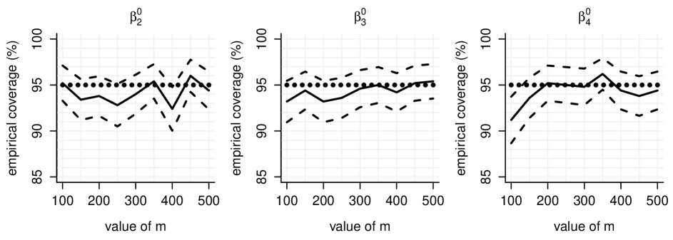
Figure S.1: Empirical coverage of confidence intervals from the simulation exercise described in Section 5. Each panel corresponds to a fixed effect model parameter that is not impacted by second term asymptotic improvements. The advertised coverage level is fixed at 95% and is indicated by a horizontal dotted line in each panel. The solid curves show, dependent on the number of groups $m$, the empirical coverage levels for confidence intervals that use a one-term asymptotic variance approximation. The dashed curves correspond to plus and minus two standard errors of the sample proportions. The within-group sample size, $n$, is fixed at $m/10$.

References

Jiang, J., Wand, M.P. & Bhaskaran, A. (2022). Usable and precise asymptotics for generalized linear mixed model analysis and design. Journal of the Royal Statistical Society, Series B, 84, 55–82.

Magnus, J.R. and Neudecker, H. (1979). The commutation matrix: some properties and applications. The Annals of Statistics, 7, 381–394.

Magnus, J.R. and Neudecker, H. (1999). Matrix Differential Calculus. Revised Edition. Chichester, U.K.: John Wiley & Sons.

Miyata, Y. (2004). Fully exponential Laplace approximation using asymptotic modes. Journal of the American Statistical Association, 99, 1037–1049.

Pace, L. and Salvan, A. (1997). Principles of Statistical Inference from a Neo-Fisherian Perspective. Singapore: World Scientific Publishing Company.

Wand, M.P. (2002). Vector differential calculus in statistics. The American Statistician, 56, 55–62.