Modeling Travel Behavior in Mobility Systems with an Atomic Routing Game and Prospect Theory

Abstract

In this paper, we present a game-theoretic modeling framework for studying the travel behavior in mobility systems, by incorporating prospect theory. As part of our motivation, we conducted an experiment in a scaled smart city to investigate the frequency of errors in actual and perceived probabilities of a highway route under free flow conditions. Based on these findings, we provide a game that captures how travelers distribute their traffic flows in a transportation network with splittable traffic, utilizing the Bureau of Public Roads function to establish the relationship between traffic flow and travel time cost. Given the inherent non-linearities, we propose a smooth approximation function that helps us estimate the prospect-theoretic cost functions. As part of our analysis, we characterize the best-fit parameters and derive an upper bound for the error. We then show a Nash Equilibrium existence. Finally, we present a numerical example and simulations to verify the theoretical results and demonstrate the effectiveness of our approximation.

I INTRODUCTION

Emerging mobility systems (e.g., connected and automated vehicles (CAVs), shared mobility), provide the most intriguing opportunity for enabling users to better monitor transportation network conditions and make better decisions for improving safety and transportation efficiency. The data and shared information of emerging mobility systems are associated to a new level of complexity in modeling and control [1]. The impact of selfish [2, 3, 4] or irrational social behavior in routing networks of cars has been studied in recent years. Other efforts have addressed “how people learn and make routing decisions” with behavioral dynamics [5]. It seems though that the problem of how travelers often have to make decisions under the risk of experiencing delays, especially when uncertainties directly can affect travel time in a transportation network has not been adequately approached yet. How likely is it for my route to work to meet traffic? As travelers have to make decisions that minimize their travel time or cost, it is imperative to regard the impact of cognitive biases on travel choices. As it has been shown in recent studies, human travel decision-making is influenced by various cognitive biases, which then lead to suboptimal travel choices. Hence, our problem of interest is to develop a novel game-theoretic modeling framework that focuses primarily on how travelers react to travel risks/uncertainties and how they perceive “mobility gains/losses” with respect to time.

In this paper, we are interested in open question: Can we develop a game-theoretic non-linear modeling framework that incorporates prospect theory for a mobility system that has at least one stable equilibrium? To address this question, we first need to understand the behavioral interactions of travelers with the network and between each other. Thus, we study the game-theoretic interactions of travelers seeking to travel in a transportation network comprised of roads using cars. A key characteristic of our approach is that we incorporate prospect theory, a human behavioral model that captures the decision-makers’ perceptions of the payoffs they might receive and how likely these payoffs are to happen.

Most of the existing game-theoretical literature in transportation assumes that the players’ behavior follows the rational choice theory, i.e., each player is a risk-neutral and utility maximizer. This seems to turn most transportation models quite unrealistic, as unexpected travel delays can lead to uncertainty in a traveler’s utility. More irrational decision-making over uncertainties and risks in utility can play a significant role, and its study can help us understand how large-scale systems perform inefficiently. There is strong evidence with empirical experiments that show how humans’ choices and preferences systematically may deviate from the choice and preferences of a game-theoretic player under the rational choice theory [6]. This is because real-life decision-making is rarely truly rational, and biases affect how we make decisions. For example, humans compare the outcomes of their choices to a known expected amount of utility (called reference) and decide based on that reference whether their utility is a gain or loss. Prospect theory has laid down the theoretical foundations to study such biases and the subjective perception of risk in utility of humans (see the seminal papers [6, 7]). Prospect theory has been recognized as a closer-to-reality behavioral model for the decision-making of humans and has been used in a wide range of applications and fields, including recent studies in engineering and transportation [8, 9, 10].

A standard approach to alleviate congestion in a transportation system has been the management of demand size due to the shortage of space availability and scarce economic resources. Such an approach focuses primarily on intelligent and scalable traffic routing, in which the objective is to optimize the routing decisions in a transportation network [11]. Game theory has been one of the standard tools that can help us investigate the impact of selfish routing on efficiency and congestion [12] and assign travelers routes to minimize travel time under a NE [13, 14, 15, 16, 17]. An important and key theoretical approach in alleviating congestion is routing/congestion games [18, 19], which are a generalization of the standard resource-sharing game of an arbitrary number of resources in a network with a number of travelers.

For our purposes, we study a prospect-theoretic game-theoretic modeling framework that combines an atomic splittable routing game with prospect theory to study travel behavior in mobility systems. We consider a finite set of travelers in a transportation network with a unique origin-destination pair. Under prospect theory with Prelec’s probability weighting function and a S-shaped value function, we can model how travelers might perceive traffic uncertainties and how they may perceive their travel gains and losses. However, prospect theory introduces rather formidable mathematical intractabilities. Thus, to address this issue, we propose an approximation smooth function that successfully estimates how travelers perceive gains/losses and the estimation of probabilities in travel time costs. Part of our focus in this paper is to establish the fitness of our proposed approximation function and also to prove the existence of at least one Nash Equilibrium (NE) in pure strategies.

In this paper, we institute a novel prospect-theoretic game-theoretic model to study travel behavior in a general mobility system. Our first contribution is the incorporation of prospect theory into the model to capture a realistic version of the travelers’ decision-making regarding travel time costs. The S-shaped value function is adopted to represent the curvature of the travel time cost function and account for the travelers’ perception of gains/losses in travel time according a reference point (which we define using the US Bureau of Public Roads (BPR) function). Our second contribution is the institution of a smooth approximation function that estimates successfully the non-linear piecewise prospect-theoretic cost functions. Finally, we prove the existence of at least one NE in pure strategies, which provides a Nash flow solution for the routing game. The significance of these contributions is further validated through numerical simulations, which confirm the effectiveness of the proposed model in predicting travel behavior in the presence of uncertainties and prospect-theoretic decision-making.

The remainder of the paper is structured as follows. In Section II, we discuss the experiment we conducted with 20 human participants. In Section III, we present the mathematical formulation of the proposed game-theoretic framework. In Section IV, we derive the theoretical properties of the proposed framework, and finally, in Section V, we discuss the implementation of the proposed framework, provide a numerical example, and draw conclusions in Section VI.

II Motivational Example

It is well established in the literature that travel behavior is rather complex and a complicated part of mobility that requires sophisticated models in order to capture the “actual” travel behavior and conditions. Travelers are tasked quite frequently to engage in a mobility system and make routing decisions under uncertainties. Such decisions are influenced by a multitude of factors (e.g., individual preferences, traffic accidents, and bad weather). Travelers then may fail to interpret the probabilities of congestion or traffic accident the right way, and thus, exhibit irrational behavior or become risk-averse. A key observation is that prospect-theoretic players aim to minimize their potential/expected losses.

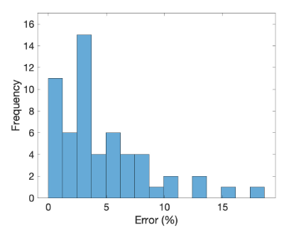
Figure 1: Frequency of errors of perceived/actual probabilities.

To better understand the factors that influence routing decisions under uncertainty, we designed and conducted an experiment with 20 participants using the Intelligent Driver Model (IDM) for all cars. We created artificial traffic congestion on different routes by controlling the speed of the preceding vehicles in a 1:25 scaled robotic testbed called IDS Lab’s Scaled Smart City (IDS3C) [20]. During the experiment the group of participants was asked to choose the route they preferred the car to take based on information provided on different traffic conditions: free flow and traffic delays. One of our key results from analyzing the data can be seen in Fig. 1. Here we have a histogram that shows the percentage error, and frequency means the number of cases. The total cases are about 60, because we had 3 different estimations for each participant. This shows that a majority of the participants failed to accurately perceive the actual probabilities of the traffic scenarios we presented to them, and most interestingly, other participants overestimated the actual probabilities by 15%. Our goal here is to understand what drives and influences a traveler’s decision as they try to minimize their travel time cost. In addition, we aim to strongly motivate a modeling that directly captures how the individuals’ perceptions of probability affect their decision-making. We leverage the results of our experiment to motivate the modeling framework in Section III.

III Modeling Framework

We consider a routing game with a finite non-empty set of players $\mathcal{I}$, $|\mathcal{I}|=n\in\mathbb{N}$. Each player $i$ represents a traveler with a connected and automated vehicle (CAV) who controls a significant amount of traffic, say $x_{i}\in\mathbb{R}_{\geq 0}$. The interpretation of this is that $x_{i}$ represents the flow of traffic that player $i$ contributes in a transportation network. We define traffic flow in this setting as the number of CAVs passing through each point in the network over time. This decision variable is non-negative as travelers make trips using the CAVs over time in the transportation network. This is in contrast to non-atomic routing games where players only control an infinitesimal amount of traffic. We also assume that traffic is splittable. Players seek to travel in the transportation network represented by a directed multigraph $\mathcal{G}=(\mathcal{V},\mathcal{E})$, where each node in $\mathcal{V}$ may represent different city areas or neighborhoods (e.g., Braess’ paradox network). Each edge $e\in\mathcal{E}$ may represent a road. For our purposes, we think of $\mathcal{G}=(\mathcal{V},\mathcal{E})$ as a representation of a smart city network with a road infrastructure that can support CAVs. Any player $i\in\mathcal{I}$ seeks to travel from an origin $o\in\mathcal{V}$ to a destination $d\in\mathcal{V}$. So, all players are associated with the same unique origin-destination pair $(o,d)\in\mathcal{V}\times\mathcal{V}$. Next, each player may use a sequence of edges that connects the OD pair $(o,d)$. We have $\mathcal{R}^{(o,d)}\subset 2^{\mathcal{E}}$ to denote the set of routes available to any player $i\in\mathcal{I}$, where each route $r_{i}$ consists of a sequence of edges connecting the origin-destination pair $(o,d)$. We are interested in how such players may compete over the routes in the network for routing their traffic flows (e.g., this is a multiple-route traffic flow decision-making problem).

We say that each player $i\in\mathcal{I}$ seeks to route their traffic in $\mathcal{G}$ represented by a traffic flow $x_{i}$ where each of its elements take values in $\mathbb{R}_{\geq 0}$. For each $i\in\mathcal{I}$, the set of actions is

$$\mathcal{X}_{i}=\left\{x_{i}\in\mathbb{R}_{\geq 0}^{|\mathcal{R}|}:\sum_{r_{i}\in\mathcal{R}}x_{i}^{r_{i}}=\bar{x}_{i}\right\},$$ (1)

where $x_{i}=(x_{i}^{r_{i}^{1}},x_{i}^{r_{i}^{2}},\dots,x_{i}^{r_{i}^{|\mathcal{R}|}})$, $\bar{x}_{i}\in\mathbb{R}_{\geq 0}$, is the total flow of player $i$, and $r_{i}^{k}$ denotes the $k$th route in the network. We write $\mathcal{X}=\mathcal{X}_{1}\times\mathcal{X}_{2}\times\dots\times\mathcal{X}_{n}$ for the Cartesian product of all the players’ action sets. We also write $x_{-i}=(x_{1},x_{2},\dots,x_{i-1},x_{i+1},\dots,x_{n})$ for the action profile that excludes player $i\in\mathcal{I}$. Next, for the aggregate action profile, we write $x=(x_{i},x_{-i})$, $x\in\mathcal{X}$.

Definition 1.

The flow on edge $e\in\mathcal{E}$ is the sum of the part of all players’ traffic flows that have chosen a route that includes edge $e$, i.e., $f_{e}(x)=\sum_{i\in\mathcal{I}}\sum_{r_{i}\ni e}x_{i}^{r_{i}}$.

In our routing game where each player $i\in\mathcal{I}$ chooses their own traffic demand vector $x_{i}$ over a common set of paths $\mathcal{R}$, if player $i$ chooses to send a traffic demand $x_{i}^{r_{i}}$ along route $r_{i}$, then this traffic demand will be distributed along all the edges in the route $r_{i}$. This is because the traffic demand on a particular route $r_{i}$ is a single quantity that is distributed among the edges in the route. Therefore, if player $i$ chooses to send a traffic demand $x_{i}(r_{i})$ along route $r_{i}$, this traffic demand will be split among all the edges $e$ in the path $p_{i}$ that player $i$ uses.

Next, we introduce a travel time latency function to capture the cost that players may experience. Intuitively, we capture the players’ preferences of different outcomes using a “cost function,” in which players are expected to act as cost minimizers. For each $e\in\mathcal{E}$, we consider non-negative cost functions $c_{e}:\mathbb{R}_{\geq 0}\to\mathbb{R}_{\geq 0}$. We assume that the cost functions at each edge $e$ are convex, continuous, and differentiable with respect to $f_{e}$. One standard way to define in an exact form $c_{e}$ is by the BPR function as it is a commonly used model for the relationship between flow and travel time. Mathematically, we have

$$c_{e}(f_{e})=c_{e}^{0}\left(1+\frac{3}{20}\left(\frac{f_{e}}{f_{e}^{CRT}}\right)^{4}\right),$$ (2)

where for any edge $e\in\mathcal{E}$, $c_{e}^{0}$ is the free-flow travel time and $f_{e}^{CRT}$ is the critical capacity of traffic flow on road $e$. We note that the BPR function is non-linear, continuous, differentiable, strictly increasing, and strictly convex for $f_{e}\geq 0$.

Definition 2.

If the maximum flow on edge $e\in\mathcal{E}$ is $f_{e}^{\max}\in\mathbb{R}_{>0}$, then for the critical flow, $f_{e}^{CRT}$, on edge $e\in\mathcal{E}$ we have $f_{e}^{CRT}<f_{e}^{\max}$.

Next, for some route $r_{i}$ of any player $i$, its cost is the sum of the costs on the edges that constitute route $r_{i}$, i.e., $c_{r_{i}}(x)=\sum_{e\in r_{i}}c_{e}(f_{e}(x))$. Now, the total cost of some player $i$ is

$$c_{i}(x)=\sum_{r_{i}\in\mathcal{R}}c_{r_{i}}(x)=\sum_{r_{i}\in\mathcal{R}}\left[\sum_{e\in r_{i}}c_{e}(f_{e})\right],$$ (3)

which simplifies to $c_{i}(x)=\sum_{r_{i}\in\mathcal{R}}\sum_{e\in r_{i}}c_{e}(f_{e})$.

Definition 3.

The game is fully characterized by the tuple $\mathcal{M}=\langle\mathcal{I},(\mathcal{X}_{i})_{i\in\mathcal{I}},(c_{i})_{i\in\mathcal{I}}\rangle$, a collection of sets of players, actions, and a profile of costs. This game is a simultaneous-move game where players make decisions at the same time and commute in $(o,d)$ of network $\mathcal{G}$.

The game $\mathcal{M}$ is a non-cooperative routing game with a transportation network and continuous action sets. Players are behaving according to prospect theory and aim to minimize their cost (e.g., travel time latencies). Naturally, players compete with each other over the available yet limited routes and how to utilize them in the transportation network. Indirectly, players make route choice that satisfy their travel needs (modeled in the form of traffic flow).

Next, we clarify “who knows what?” in our routing game. All players have complete knowledge of the game and the network. Each player knows their own information (action and cost) as well as the information of other players. At equilibrium, we want to ensure that no player has an incentive to unilaterally deviate from their chosen decisions and change how they distribute their traffic flows over the available routes in the network. So, for the purposes of our work, we observe that a NE in pure strategies is most fitting to apply as a solution concept. We formally define a NE in terms of the players’ traffic flows.

Definition 4.

A feasible flow profile $x^{*}=(x_{i}^{r_{i}})_{i\in\mathcal{I}}^{r_{i}\in\mathcal{R}}\in\mathcal{X}$ constitutes a NE if for each player $i\in\mathcal{I}$, $c_{i}(x_{i}^{*},x_{-i}^{*})\leq c_{i}(x_{i},x_{-i}^{*})$, for all $x_{i}\in\mathcal{X}_{i}$.

In other words, a flow profile $x^{*}$ is a NE if no player can reduce their total cost by unilaterally changing how they distribute their total traffic flow over the available routes in the network. In a NE, each player’s specific $x_{i}$ has the lowest possible cost among all possible distributions over the routes, given the choices made by other players.

III-A Prospect Theory Analysis

In this subsection, we provide a brief introduction to prospect theory and its main concepts [21]. One of the main questions prospect theory attempts to answer is how a decision-maker may evaluate different possible actions/outcomes under uncertain and risky circumstances. Thus, prospect theory is a descriptive behavioral model and focuses on three main behavioral factors: (i) Reference dependence: decision makers make decisions based on their utility, which is measured from the “gains” or “losses.” However, the utility is a gain or loss relative to a reference point that may be unique to each decision maker. (ii) Diminishing sensitivity: changes in value have a greater impact near the reference point than away from the reference point. (iii) Loss aversion: decision makers are more conservative in gains and more risky in losses. One way to mathematize the above behavioral factors (1) - (3), is to consider an action by a decision-maker as a “gamble” with objective utility value $z\in\mathbb{R}$. We say that this decision maker perceives $z$ subjectively using a value function [7, 22]

$$v(z)=\begin{cases}(z-z_{0})^{\beta_{1}},&\text{if }z\geq z_{0},\\ -\lambda(z_{0}-z)^{\beta_{2}},&\text{if }z<z_{0},\end{cases}$$ (4)

where $z_{0}$ represents a reference point, $\beta_{1},\beta_{2}\in(0,1)$ are parameters that represent the diminishing sensitivity. Both $\beta_{1},\beta_{2}$ shape (4) in a way that the changes in value have a greater impact near the reference point than away from the reference point. We observe that (4) is concave in the domain of gains and convex in the domain of losses. Moreover, $\lambda\geq 1$ reflects the level of loss aversion of decision makers. To the best of our knowledge, there does not exists a widely-agreed theory that determines and defines the reference dependence [6]. In engineering [23, 10], it is assumed that $z_{0}=0$ capturing a decision-maker’s expected status-quo level of the resources.

Prospect theory models the subjective behavior of decision makers under uncertainty and risk. Each objective utility $z\in\mathbb{R}$ is associated with a probabilistic occurrence, say $p\in[0,1]$. Decision makers though are subjective and perceive $p$ in different ways depending on its value. To capture this behavior, we introduce a strictly increasing function $w:[0,1]\to[0,1]$ with $w(0)=0$ and $w(1)=1$ called the probability weighting function. This function allows us to model how decision makers may overestimate small probabilities of objective utilities, i.e., $w(p)>p$ if $p$ is close to $0$, or underestimate high probabilities, i.e., $w(p)<p$ if $p$ is close to $1$. For the purposes of this work, we use the probability weighting function first introduced in [24], $w(p)=\exp\left(-(-\log(p))^{\beta_{3}}\right),\quad p\in[0,1]$, where $\beta_{3}\in(0,1)$ represents a rational index, i.e., the distortion of a decision-maker’s probability perceptions. Mathematically, $\beta_{3}$ controls the curvature of the weighting function. Next, we define a prospect which is a tuple of the objective utility (gain or loss) and its probability of happening.

Definition 5.

Suppose that there are $K\in\mathbb{N}$ possible outcomes available to a decision-maker and $z_{k}\in\mathbb{R}$ is the $k$th gain/loss of objective utility. Then a prospect $\ell_{k}$ is a tuple of the utilities and their respective probabilities $\ell_{k}=(z_{0},z_{1},z_{2},\dots,z_{K};p_{0},p_{1},p_{2},\dots,p_{K})$, where $k=1,2,\dots,K$. We denote the $k$th prospect more compactly as $\ell_{k}=(z_{k},p_{k})$. We have that $\sum_{k=0}^{K}p_{k}=1$ and $\ell_{k}$ is well-ordered, i.e., $z_{0}\leq z_{1}\leq\cdots\leq z_{K}$. Under prospect theory, the decision-maker evaluates their “subjective utility” as $u(\ell)=\sum_{0\leq k\leq K}v(z_{k})w(p_{k})$, where $\ell=(\ell_{k})_{k=1}^{K}$ is the profile of prospects of $K$ outcomes.

In the remainder of this subsection, we apply the prospect theory to our modeling framework, clearly define the mobility outcomes (objective and subjective utilities), and then show that the prospect-theoretic game $\mathcal{M}$ admits a NE. Players may be uncertain on the value of the traffic disturbances as it is affected by unexpected factors, and so that is why we use Prelec’s probability weighting function $w:[0,1]\to[0,1]$ to capture how different traveler populations “perceive” probabilities. In addition, we are interested in capturing how players may perceive their gains or losses in terms of their travel time costs with respect to the costs at critical density. The mobility prospect is whether the $f_{e}$ will reach at most its critical point or its jammed point. Formally, $\pi_{e}$ is the probability that $f_{e}\in(0,f_{e}^{CRT})$, and $1-\pi_{e}$ is the probability for $f_{e}\in(f_{e}^{CRT},f_{e}^{\max}]$. We then use the prospect-theoretic S-shaped value function $v(c_{e}(f_{e})):\mathbb{R}_{\geq 0}\to\mathbb{R}$ to capture how players may perceive such costs. Hence, we have

$$v(c_{e}(f_{e}))=\begin{cases}\lambda(c_{e}^{0}-c_{e}(f_{e}))^{\beta},&\text{if }c_{e}(f_{e})\leq c_{e}^{0},\\ -(c_{e}(f_{e})-c_{e}^{0})^{\beta},&\text{if }c_{e}(f_{e})>c_{e}^{0},\end{cases}$$ (5)

where the reference dependence is represented by $c_{e}^{0}=c_{e}(f_{e}^{CRT})$, $\beta_{1}=\beta_{2}=\beta\in(0,1)$, and for each $e\in\mathcal{E}$, we have $\pi_{e}\in[0,1]$. We can justify $\beta_{1}=\beta_{2}$ in the above definition as it has been verified to produce extremely good results and the outcomes are consistent with the original data [7]. We define

$$\tilde{c}_{e}(f_{e})=\begin{cases}c_{e}^{0}-c_{e}(f_{e}),&\text{if }c_{e}(f_{e})<c_{e}^{0},\\ c_{e}(f_{e})-c_{e}^{0},&\text{if }c_{e}(f_{e})>c_{e}^{0}.\end{cases}$$ (6)

Remark 1.

It is easy to note that our prospect-theoretic value function is “reversed” capturing the way the player will perceive the gains in travel time through a cost function. Using as a reference point the critical traffic flow on edge $e$, we can pinpoint the exact point that any more delays become socially unacceptable, i.e., a higher flow causes a higher travel time that the traveler will not tolerate.

Under prospect theory the new “cost function” is given by

$$c_{e}^{\text{PT}}(f_{e})=w(\pi_{e})\cdot\lambda\cdot[\tilde{c}_{e}(f_{e}\,|\,c_{e}(f_{e})<c_{e}^{0})]^{\beta}\\ -w(1-\pi_{e})\cdot[\tilde{c}_{e}(f_{e}\,|\,c_{e}(f_{e})>c_{e}^{0})]^{\beta}.$$ (7)

The total cost on some route $r_{i}$ for player $i$ under prospect theory is $c_{r_{i}}^{\text{PT}}(x)=\sum_{e\in r_{i}}c_{e}^{\text{PT}}(f_{e})$. Now, the total cost of some player $i$ is given by

$$c_{i}^{\text{PT}}(x)=\sum_{r_{i}\in\mathcal{R}}\sum_{e\in r_{i}}c_{e}^{\text{PT}}(f_{e}).$$ (8)

Note, however, that in this case the prospect-theoretic cost is capturing the gains and losses of a traveler. Thus, the aim is to maximize this function in order to maximize the gains. In other words, by minimizing the actual cost, we maximize the perceived gains in travel time by the traveler.

What we observe in (8) is that it is rather cumbersome to analyze it in game theory as issues in the smoothness of the function arise quickly. The key problem in analyzing such a function is that the exponent takes values in $(0,1)$. However, we propose a new function that approximates the prospect-theoretic function and, most importantly, can be shown to have useful properties. Hence, we define the following function

$$\sigma(f_{e})=\frac{\delta_{1}}{1+\exp{\left(\frac{\delta_{2}-f_{e}}{\delta_{3}}\right)}}+\delta_{4},$$ (9)

where $\delta_{1},\delta_{2},\delta_{3},\delta_{4}\in\mathbb{R}$, and $f_{e}\in[0,f_{e}^{\max}]$. So, we can write

$$c_{i}^{\text{PT}}(x)=\sum_{r_{i}\in\mathcal{R}}\sum_{e\in r_{i}}\sigma(f_{e}).$$ (10)

IV Analysis and Properties of the Game

In this section, we provide a formal analysis of the properties of our proposed modeling framework and show that our game admits a NE in pure strategies.

Lemma 1.

The strategy space of the game $\mathcal{M}$ is non-empty, compact, and convex.

Proof.

To show that the set $\mathcal{X}_{i}=\{x_{i}\in\mathbb{R}_{\geq 0}^{|\mathcal{R}|}:\sum_{r_{i}\in\mathcal{R}}x_{i}^{r_{i}}=\bar{x}_{i}\}$ is non-empty, compact, and convex, we need to examine each property individually. (i) Non-empty: Consider the strategy where player $i$ allocates all of their traffic, $\bar{x}_{i}$, to a single route, say $r_{1}$, and allocates zero traffic traffic to the remaining routes. Then, we have $x_{i}=(\bar{x}_{i},0,\dots,0)\in\mathbb{R}_{\geq 0}^{|\mathcal{R}|}$, which satisfies the constraint: $\sum_{r_{i}\in\mathcal{R}}x_{i}^{r_{i}}=\bar{x}_{i}$. Thus, $\mathcal{X}_{i}$ is non-empty for every player $i\in\mathcal{I}$. (ii) Compact: To show that $\mathcal{X}_{i}$ is bounded and closed, we only need to note that for each $x_{i}\in\mathcal{X}_{i}$, we must have $0\leq x_{i}^{r_{i}}\leq\bar{x}_{i}$ for any route $r_{i}$. (iii) Convex: We need to show that for each player $i\in\mathcal{I}$, the set $\mathcal{X}_{i}$ is convex, i.e., for any $x_{i},y_{i}\in\mathcal{X}_{i}$ and any $\mu\in[0,1]$, we have $\mu x_{i}+(1-\mu)y_{i}\in\mathcal{X}_{i}$. Let $x_{i},y_{i}\in\mathcal{X}_{i}$ and $\lambda\in[0,1]$. We want to show that $z_{i}=\lambda x_{i}+(1-\lambda)y_{i}\in\mathcal{X}_{i}$. We know that $x_{i},y_{i}\in\mathcal{X}_{i}$ satisfy the constraint: $\sum_{r_{i}\in\mathcal{R}}x_{i}^{r_{i}}=\bar{x}_{i}$ and $\sum_{r_{i}\in\mathcal{R}}y_{i}^{r_{i}}=\bar{x}_{i}$. Now, consider the weighted sum:

$$\sum_{r_{i}\in\mathcal{R}}z_{i}^{r_{i}} =\sum_{r_{i}\in\mathcal{R}}(\mu x_{i}^{r_{i}}+(1-\mu)y_{i}^{r_{i}})$$

$$=\mu\sum_{r_{i}\in\mathcal{R}}x_{i}^{r_{i}}+(1-\mu)\sum_{r_{i}\in\mathcal{R}}y_{i}^{r_{i}}$$

$$=\mu\bar{x}_{i}+(1-\mu)\bar{x}_{i}=\bar{x}_{i}.$$ (11)

Since $z_{i}$ also satisfies the constraint, we have $z_{i}\in\mathcal{X}_{i}$. Therefore, $\mathcal{X}_{i}$ is convex for each player $i\in\mathcal{I}$. In conclusion, for each player $i\in\mathcal{I}$, the strategy space $\mathcal{X}_{i}$ is non-empty, compact, and convex. ∎

Next, we characterize the coefficients of $\sigma$ function.

Lemma 2.

The approximation function given by (9) in the interval $[0,\kappa]$, $\kappa<f_{e}^{\max}$, is strictly concave with respect to $f_{e}$ when $\delta_{3}>0$, $\delta_{4}\in\mathbb{R}$, and (i) $\delta_{1}>0$, $\delta_{2}>f_{e}$, or alternatively (ii) $\delta_{1}<0$, $\delta_{2}<f_{e}$.

Proof.

Given that $f_{e}\geq 0$, we analyze the second-order derivative of the function $\sigma(f_{e})=\frac{\delta_{1}}{1+\exp{\left(\frac{\delta_{2}-f_{e}}{\delta_{3}}\right)}}+\delta_{4}$ to determine the conditions for strict concavity. First, let us find the first and second-order derivatives of $\sigma$ with respect to $f_{e}$, i.e.,

$$\sigma^{\prime}(f_{e}) =\frac{-\delta_{1}\exp{(\frac{\delta_{2}-f_{e}}{\delta_{3}})}}{\delta_{3}(1+\exp{(\frac{\delta_{2}-f_{e}}{\delta_{3}})})^{2}},$$ (12)

$$\sigma^{\prime\prime}(f_{e}) =\frac{2\delta_{1}\exp{(\frac{\delta_{2}-f_{e}}{\delta_{3}})}(1-\exp{(\frac{\delta_{2}-f_{e}}{\delta_{3}})})}{\delta_{3}^{2}(1+\exp{(\frac{\delta_{2}-f_{e}}{\delta_{3}})})^{3}}.$$ (13)

Now, we examine the conditions for $\sigma^{\prime\prime}(f_{e})<0$. First, $\delta_{1}$ controls the sign of the second-order derivative as follows: if $\delta_{1}<0$ and $\delta_{3}>0$, $\sigma^{\prime\prime}(f_{e})$ will be negative when $1-\exp{(\frac{\delta_{2}-f_{e}}{\delta_{3}})}<0$, which simplifies to $\delta_{2}>f_{e}$. If $\delta_{3}<0$ in either of the cases, then the signs are reversed. We do require though that $\delta_{3}^{2}$ is well-defined, so $\delta_{3}\neq 0$. On greater detail, $1-\exp{(\frac{\delta_{2}-f_{e}}{\delta_{3}})}$ determines the conditions for $\sigma^{\prime\prime}(f_{e})$ to be negative. If $\delta_{1}<0$, we need $1-\exp{(\frac{\delta_{2}-f_{e}}{\delta_{3}})}>0$, which implies that $f_{e}>\delta_{2}-\delta_{3}\log{(1)}$ (since $f_{e}\geq 0$). If $\delta_{1}<0$, we need $1-\exp{(\frac{\delta_{2}-f_{e}}{\delta_{3}})}<0$, which implies that $f_{e}<\delta_{2}-\delta_{3}\log{(1)}$.

Combining these insights, we can conclude that the function $\sigma(f_{e})=\frac{\delta_{1}}{1+\exp{(\frac{\delta_{2}-f_{e}}{\delta_{3}})}}+\delta_{4}$ becomes strictly concave in the entire interval. So, it is strictly concave for $f_{e}\geq 0$ if: (i) $\delta_{1}>0,\delta_{3}>0$ and $f_{e}<\delta_{2}$; (ii) $\delta_{1}<0$, $\delta_{3}>0$, and $f_{e}>\delta_{2}$. If $\delta_{3}<0$, then the relation between $f_{e}$ and $\delta_{2}$ is naturally reversed. Note that the parameter $\delta_{4}$ does not affect the convexity of the function, as it only shifts the function vertically. Therefore, we have derived the necessary conditions that ensure $\sigma^{\prime\prime}(f_{e})$ is negative for all $f_{e}$ making $\sigma(f_{e})$ strictly concave. ∎

It follows easily that it is strictly decreasing, continuous, and (continuously) differentiable with respect to the traffic flow $f_{e}\in[0,f_{e}^{\max}]$ for any edge $e\in\mathcal{E}$.

Now we provide a discussion for the error characterization of our approximation function. Let us define the error function $\Phi$ as the squared difference between $c_{e}^{\text{PT}}(f_{e})$ and $\sigma(f_{e})$, integrated over the interval $[0,\kappa]$:

$$\Phi(\delta_{1},\delta_{2},\delta_{3},\delta_{4})=\int_{0}^{\kappa}\left(c_{e}^{\text{PT}}(f_{e})-\sigma(f_{e})\right)^{2}\mathrm{d}x.$$ (14)

The goal is to minimize $\Phi$ with respect to the parameters $\delta_{1},\delta_{2},\delta_{3}$, and $\delta_{4}$. First we find the critical points of $\Phi$ by setting its gradient to zero and solving the resulting system of equations: $\nabla\Phi(\delta_{1},\delta_{2},\delta_{3},\delta_{4})=0$. This results in a system of equations involving the partial derivatives of $\Phi$ with respect to each of the parameters, i.e., $\frac{\partial\Phi}{\partial\delta_{1}}=0,\quad\frac{\partial\Phi}{\partial\delta_{2}}=0,\frac{\partial\Phi}{\partial\delta_{3}}=0$, and $\frac{\partial\Phi}{\partial\delta_{4}}=0$. To compute these partial derivatives, we need to differentiate the integrand with respect to each parameter and then integrating it again, for example: $\frac{\partial\Phi}{\partial\delta_{1}}=\int_{0}^{\kappa}\frac{\partial}{\partial\delta_{1}}\left(c_{e}^{\text{PT}}(f_{e})-\sigma(f_{e})\right)^{2}\mathrm{d}x$. This process needs to be repeated for all parameters. However, due to the complexity of the function $c_{e}^{\text{PT}}(f_{e})$ (being a non-linear piecewise function), it is not possible to obtain an explicit analytical expression for these partial derivatives. For our purposes, we rely on numerical optimization techniques to find the exact best-fit parameters that minimize the error function, as these methods can handle easily the complex and non-linear optimization. In the next subsection, we provide a numerical example that showcases the efficacy of the approximation function.

Theorem 1.

The error $\phi(\cdot)=\left(c_{e}^{\text{PT}}(f_{e})-\sigma(f_{e})\right)$ is upper bounded by $\gamma+\varepsilon$, where $\gamma$ is some real number and $\varepsilon>0$.

Proof.

For the purposes of this proof we assume that $\beta=0.5$, $\lambda=2$ and $c_{e}^{0}=13$ and $f_{e}^{\text{CRT}}=1$ and $c_{e}^{0}=14.95$. We substitute now the known equations to get $\phi(\delta_{1},\delta_{2},\delta_{3},\delta_{4})=-w(1-\pi_{e})\cdot[\tilde{c}_{e}(f_{e}\,|\,c_{e}(f_{e})>c_{e}^{0})]^{\beta}-\frac{\delta_{1}}{1+\exp{\left(\frac{\delta_{2}-f_{e}}{\delta_{3}}\right)}}-\delta_{4}$. Using a straightforward computation of the second-order derivative we can get the inflection point of $\phi$, which will lie in $(1,1+\varepsilon)$. This means that it is sufficient for us to compute $\phi$ at $f_{e}=1$, and focus on $\phi$ for $f_{e}>1$. Since $\sigma$ is smooth and strictly concave in that interval it approximates the worst $c_{e}^{\text{PT}}$ around the inflection point. So, we have the following $\phi(\delta_{1},\delta_{2},\delta_{3},\delta_{4})=-w(1-\pi_{e})(c_{e}(f_{e})-c_{e}^{0})^{\beta}-\frac{\delta_{1}}{1+\exp{\left(\frac{\delta_{2}-f_{e}}{\delta_{3}}\right)}}-\delta_{4}$. This expression simplifies to

$$\phi=-w(1-\pi_{e})\left[13\Bigg{(}1+\frac{3}{20}(f_{e})^{4}\Bigg{)}-14.95\right]^{\beta}\\ -\frac{\delta_{1}}{1+\exp{\left(\frac{\delta_{2}-f_{e}}{\delta_{3}}\right)}}-\delta_{4},$$ (15)

where we have $\delta_{1}<0$ and $\delta_{2},\delta_{3},\delta_{4}>0$, and $\delta_{2}>f_{e}$. Since $w(1-\pi_{e})$ is only a positive parameter constant, it is negligible, and so we drop it from our analysis. The first component simplifies to $\left[\frac{39}{20}\left(1-(f_{e})^{4}\right)\right]^{\beta}$, which is negative when we evaluate near the inflection point. Next, it follows that the second component is positive for small values of $\delta_{2}$ and $\delta_{3}$. We use the Taylor series expansion evaluated at $f_{e}=1+\varepsilon$, where $\varepsilon$ is a small positive number to get

$$-\left[\frac{39}{20}\left((f_{e})^{4}-1\right)\right]^{\beta}=\\ -\sqrt{\frac{39}{5}}\sqrt{\varepsilon}-\frac{3}{4}\frac{\sqrt{39}}{5}\varepsilon^{\frac{3}{2}}-\frac{7}{32}\frac{\sqrt{39}}{5}\varepsilon^{\frac{5}{2}}+O(\varepsilon^{\frac{7}{2}}),$$ (16)

which is clearly negative. For the second component, we use the Taylor series expansion again at the same point $f_{e}=1+\varepsilon$, and get the following

$$\frac{\delta_{1}}{1+\exp{\left(\frac{\delta_{2}-(1+\varepsilon)}{\delta_{3}}\right)}}=\frac{\delta_{1}}{1+\exp{\left(\frac{\delta_{2}-1}{\delta_{3}}\right)}}\\ +\frac{\delta_{1}\exp{\left(\frac{\delta_{2}-1}{\delta_{3}}\right)}}{\delta_{3}\left(1+\exp{\left(\frac{\delta_{2}-1}{\delta_{3}}\right)}\right)^{2}}\cdot\varepsilon\\ \frac{1}{2}\frac{\delta_{1}\exp{\left(\frac{1}{\delta_{3}}+\frac{\delta_{2}}{\delta_{3}}\right)}\left(\exp{\left(\frac{1}{\delta_{3}}\right)}-\exp{\left(\frac{\delta_{2}}{\delta_{3}}\right)}\right)}{\delta_{3}^{2}\left(\exp{\left(\frac{1}{\delta_{3}}\right)}+\exp{\left(\frac{\delta_{2}}{\delta_{3}}\right)}\right)^{3}}\cdot\varepsilon^{2}+O(\varepsilon^{3})$$ (17)

We combine the expressions for the first and second components. From what we have established so far we get that the error is given by

$$\phi=-\sqrt{\frac{39}{5}}\sqrt{\varepsilon}-\frac{3}{4}\frac{\sqrt{39}}{5}\varepsilon^{\frac{3}{2}}-\frac{7}{32}\frac{\sqrt{39}}{5}\varepsilon^{\frac{5}{2}}+O(\varepsilon^{\frac{7}{2}})\\ +\frac{\delta_{1}}{1+\exp{\left(\frac{\delta_{2}-1}{\delta_{3}}\right)}}+\frac{\delta_{1}\exp{\left(\frac{\delta_{2}-1}{\delta_{3}}\right)}}{\delta_{3}\left(1+\exp{\left(\frac{\delta_{2}-1}{\delta_{3}}\right)}\right)^{2}}\cdot\varepsilon\\ +\frac{1}{2}\frac{\delta_{1}\exp{\left(\frac{1}{\delta_{3}}+\frac{\delta_{2}}{\delta_{3}}\right)}\left(\exp{\left(\frac{1}{\delta_{3}}\right)}-\exp{\left(\frac{\delta_{2}}{\delta_{3}}\right)}\right)}{\delta_{3}^{2}\left(\exp{\left(\frac{1}{\delta_{3}}\right)}+\exp{\left(\frac{\delta_{2}}{\delta_{3}}\right)}\right)^{3}}\cdot\varepsilon^{2}+O(\varepsilon^{3}).$$ (18)

We want to find an upper bound for the error, which means we need to show that (18) is less than or equal to $\gamma+\varepsilon$ for some $\gamma\in\mathbb{R}$. Note that for any $a,b\in\mathbb{R}$ with $a<0$ and $b>0$, it is always true that $a+b\leq\max\{a,b\}$. Thus, we can write

$$\phi\leq\max\bigg{\{}-\sqrt{\frac{39}{5}}\sqrt{\varepsilon}-\frac{3}{4}\frac{\sqrt{39}}{5}\varepsilon^{\frac{3}{2}}-\frac{7}{32}\frac{\sqrt{39}}{5}\varepsilon^{\frac{5}{2}}+O(\varepsilon^{\frac{7}{2}}),\\ \frac{\delta_{1}}{1+\exp{\left(\frac{\delta_{2}-1}{\delta_{3}}\right)}}+\frac{\delta_{1}\exp{\left(\frac{\delta_{2}-1}{\delta_{3}}\right)}}{\delta_{3}\left(1+\exp{\left(\frac{\delta_{2}-1}{\delta_{3}}\right)}\right)^{2}}\cdot\varepsilon\\ +\frac{1}{2}\frac{\delta_{1}\exp{\left(\frac{1}{\delta_{3}}+\frac{\delta_{2}}{\delta_{3}}\right)}\left(\exp{\left(\frac{1}{\delta_{3}}\right)}-\exp{\left(\frac{\delta_{2}}{\delta_{3}}\right)}\right)}{\delta_{3}^{2}\left(\exp{\left(\frac{1}{\delta_{3}}\right)}+\exp{\left(\frac{\delta_{2}}{\delta_{3}}\right)}\right)^{3}}\cdot\varepsilon^{2}+O(\varepsilon^{3})\bigg{\}}.$$ (19)

As $\varepsilon$ is positively small, we take the limit as $\varepsilon\to 0$. We note that the term $-\sqrt{\frac{39}{5}}\sqrt{\varepsilon}$ dominates as $\varepsilon\to 0$, and so the first component approaches $-\infty$ as $\varepsilon\to 0$. For the second component, the term $\frac{\delta_{1}}{1+\exp{\left(\frac{\delta_{2}-1}{\delta_{3}}\right)}}$ dominates as $\varepsilon\to 0$, and since $\delta_{1}<0$ and $\delta_{2},\delta_{3}>0$, the second component is positive. Therefore, we can write

$$\lim_{\varepsilon\to 0}\phi\leq\lim_{\varepsilon\to 0}\max\left\{-\sqrt{\frac{39}{5}}\sqrt{\varepsilon},\frac{\delta_{1}}{1+\exp{\left(\frac{\delta_{2}-1}{\delta_{3}}\right)}}\right\}.$$ (20)

As $\varepsilon\to 0$, we have $-\sqrt{\frac{39}{5}}\sqrt{\varepsilon}\to-\infty$, hence

$$\lim_{\varepsilon\to 0}\phi \leq\lim_{\varepsilon\to 0}\max\left\{-\sqrt{\frac{39}{5}}\sqrt{\varepsilon},\frac{\delta_{1}}{1+\exp{\left(\frac{\delta_{2}-1}{\delta_{3}}\right)}}\right\}$$

$$=\frac{\delta_{1}}{1+\exp{\left(\frac{\delta_{2}-1}{\delta_{3}}\right)}}.$$ (21)

Now, let $\gamma=\frac{\delta_{1}}{1+\exp{\left(\frac{\delta_{2}-1}{\delta_{3}}\right)}}$. Since the second component is positive, we have $\gamma>0$, thus $\phi\leq\gamma+\varepsilon$. Therefore, we have shown that the error $\phi$ is upper bounded by $\gamma+\varepsilon$, where $\gamma\in\mathbb{R}$ and $\varepsilon>0$. ∎

Lemma 3.

A traffic flow $x^{*}$ is a NE if and only if, for all $x\in\mathcal{X}$, for all $i\in\mathcal{I}$, we have $\left\langle\nabla_{i}c_{i}(x_{i}^{*},x_{-i}^{*}),x_{i}-x_{i}^{*}\right\rangle\geq 0$, where by the chain rule with respect to the $x_{i}^{r_{i}}$ we can take the partial derivatives on the cost function to get

$$\left\langle\sum_{r_{i}\in\mathcal{R}}\sum_{e\in r_{i}}\sigma^{\prime}(f_{e}^{*}),x_{i}-x_{i}^{*}\right\rangle\geq 0.$$ (22)

Proof.

We apply the chain rule with respect to the $x_{i}^{r_{i}}$ and substituting the given cost function $c_{i}(x)$ and flow $f_{e}(x)$. The traffic flow $x^{*}$ is a NE if and only if, for all $x\in\mathcal{X}$ and for all $i\in\mathcal{I}$, we have $\left\langle\nabla_{i}c_{i}(x_{i}^{*},x_{-i}^{*}),x_{i}-x_{i}^{*}\right\rangle\geq 0$, where $c_{i}(x)=\sum_{r_{i}\in\mathcal{R}}\sum_{e\in r_{i}}\sigma(f_{e})$ and $f_{e}(x)=\sum_{i}\sum_{r_{i}\ni e}x_{i}^{r_{i}}$. Now, we compute the gradient of the cost function with respect to $x_{i}$:

$$\nabla_{i}c_{i}(x_{i}^{*},x_{-i}^{*})=\sum_{r_{i}\in\mathcal{R}}\sum_{e\in r_{i}}\frac{\partial\sigma(f_{e})}{\partial x_{i}^{r_{i}}}.$$ (23)

To compute the partial derivative $\frac{\partial\sigma(f_{e})}{\partial x_{i}^{r_{i}}}$, we use the chain rule: $\frac{\partial\sigma(f_{e})}{\partial x_{i}^{r_{i}}}=\sigma^{\prime}(f_{e})\cdot\frac{\partial f_{e}}{\partial x_{i}^{r_{i}}}$, where $\sigma^{\prime}(f_{e})$ is the derivative of the function $\sigma$ with respect to $f_{e}$. Since $f_{e}(x)=\sum_{i}\sum_{r_{i}\ni e}x_{i}^{r_{i}}$, we have $\frac{\partial f_{e}}{\partial x_{i}^{r_{i}}}=1$. Now, we can substitute this back into the gradient expression $\nabla_{i}c_{i}(x_{i}^{*},x_{-i}^{*})=\sum_{r_{i}\in\mathcal{R}}\sum_{e\in r_{i}}\sigma^{\prime}(f_{e}^{*})$. Finally, we can rewrite the NE condition using the gradient

$$\left\langle\sum_{r_{i}\in\mathcal{R}}\sum_{e\in r_{i}}\sigma^{\prime}(f_{e}^{*}),x_{i}-x_{i}^{*}\right\rangle\geq 0.$$ (24)

This is the necessary and sufficient first-order condition for $x_{i}^{*}$ of any player $i$ to be a minimum of cost function $c_{i}(\cdot)$. ∎

Theorem 2.

The game $\mathcal{M}$ admits at least one NE.

Proof.

We formally prove the existence of a NE in the prospect-theoretic routing game using Brouwer’s fixed point theorem. Recall that for any player $i$, $c_{i}^{\text{PT}}(x)=\sum_{r_{i}\in\mathcal{R}}\sum_{e\in r_{i}}\sigma(f_{e}(x))$, where $\sigma$ is our smooth and monotonic approximation function. We define the best-response correspondence for each player $i$ as: $b_{i}(x_{-i})=\arg\max_{x_{i}}c_{i}^{\text{PT}}(x)$. Smoothness in the approximation function $\sigma$ implies that it is continuous and has continuous derivatives. This implies that we can estimate the utility function $c_{i}^{\text{PT}}(x)$ continuously with respect to the traffic vector $x$. To show that the best-response correspondence $b_{i}(x_{-i})$ is continuous, we need the $\arg\max$ operator to be continuous. Since the set of maximizers is compact, which actually follows from the compactness of the strategy space by Lemma 1. By Lemma 2, we have that $\sigma$ is concave on a specific interval $[0,\kappa]$. This implies that we can estimate the utility function $c_{i}^{\text{PT}}(x)$ within the interval $[0,\kappa]$ pointwise in a strictly decreasing and concave curve with respect to $x_{i}$ for any player $i\in\mathcal{I}$. However, a strictly concave function has at most one unique maximum, which ensures the single-valuedness of the best-response correspondence $b_{i}(x_{-i})$. We now define the combined best-response correspondence $B(x)=(b_{1}(x_{-1}),b_{2}(x_{-2}),\dots,b_{n}(x_{-n}))$. Since each $b_{i}(x_{-i})$ is continuous, $B(x)$ is also continuous, and thus it maps the strategy space to itself. Hence now we can apply Brouwer’s fixed point theorem, which guarantees that there exists a fixed point $x^{*}=B(x^{*})$; the result then follows. ∎

V SIMULATION RESULTS

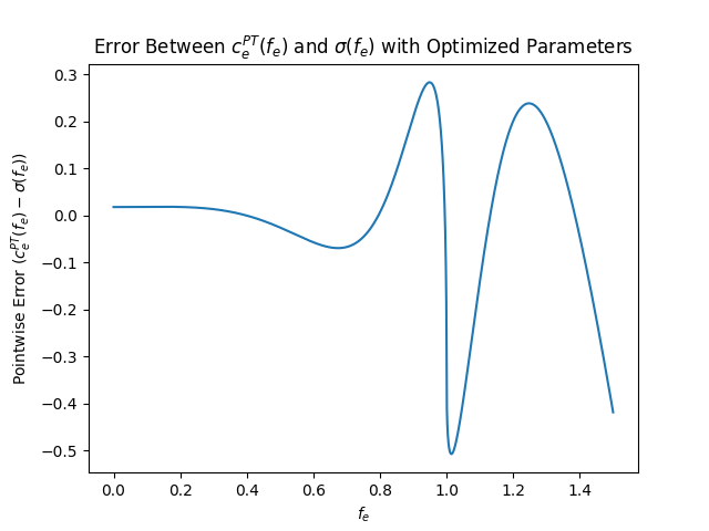
Figure 2: The plot of the errors.

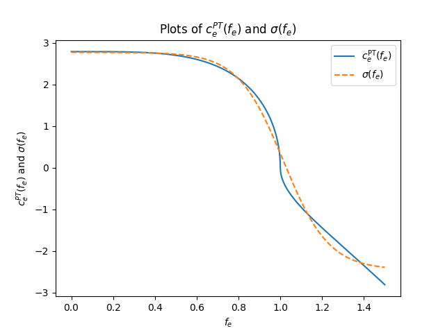
Figure 3: The plot of the original and approximation functions.

In this section, we offer a numerical example to showcase the efficacy of our approach. We used the Broyden-Fletcher-Goldfarb-Shanno (BFGS) algorithm to minimize the error between function $c_{e}^{\text{PT}}(\cdot)$ and our approximation function $\sigma(\cdot)$ on the interval $[0,3/2]$. We used the SciPy optimization function minimize() with the BFGS method to find the optimized parameters for $\sigma(\cdot)$ that minimize pointwise the smallest sum of squared errors. Table I shows the optimized parameters found by the BFGS algorithm, and Table I shows the error bound on the interval $[0,3/2]$. The maximum error was 0.5072, the minimum error was 0, and the average error was 0.1043. These results provide an important summary of the performance of our approximation function and the best-fit parameters in estimating the prospect-theoretic function $c_{e}^{\text{PT}}(\cdot)$.

Parameter	Value
$\delta_{1}$	-5.232
$\delta_{2}$	1.015
$\delta_{3}$	0.109
$\delta_{4}$	2.776

(a) Optimized Parameters.

Error Measure	Value
Maximum Error	0.5072
Minimum Error	0.0000
Average Error	0.1043

(b) Error Bound on $[0,3/2]$.

TABLE I: Summarizing the parameters of the numerical example and the average/range of the error.

VI CONCLUSIONS AND FUTURE WORK

In this paper, we presented a prospect-theoretic game-theoretic modeling framework that incorporates an atomic splittable routing game with prospect theory to study travel behavior in mobility systems. We modeled the overestimation/underestimation of probabilities using Prelec’s probability weighting function and we took into account the traffic uncertainties and travelers’ perception of gains/losses in travel time using a prospect-theoretic S-shaped value function. We proposed an approximation function to address the non-linear and piecewise nature of the prospect-theoretic cost functions and showed that at least one NE exists. In addition, we derived an upper bound for the error. Lastly, we provided a numerical example and demonstrated the efficacy of our approximation for the routing game and summarized our results the best-fit parameters and range/average errors.

In future research, we can explore how to analyze a convex-concave piecewise non-linear optimization problem using advanced optimization techniques, such as sequential convex programming or cutting plane methods. The development of such an optimization framework can enhance our ability to predict travel decisions in mobility systems under prospect theory. Another direction is to incorporating prospect theory and a taxation mechanism and studying how we can incentivize prospect-theoretic travelers and the trade-offs of efficiency in the mobility systems [25, 26].

References

- [1] A. A. Malikopoulos, “A duality framework for stochastic optimal control of complex systems,” IEEE Transactions on Automatic Control, vol. 61, no. 10, pp. 2756–2765, 2016.
- [2] N. Mehr and R. Horowitz, “How will the presence of autonomous vehicles affect the equilibrium state of traffic networks?” IEEE Transactions on Control of Network Systems, vol. 7(1), pp. 96–105, 2019.
- [3] D. A. Lazar, S. Coogan, and R. Pedarsani, “Routing for traffic networks with mixed autonomy,” IEEE Transactions on Automatic Control, vol. 66(6), pp. 2664–2676, 2021.
- [4] E. Bıyık, D. Lazar, R. Pedarsani, and D. Sadigh, “Incentivizing efficient equilibria in traffic networks with mixed autonomy,” IEEE Transactions on Control of Network Systems, vol. 8(4), pp. 1717–1729, 2021.
- [5] W. Krichene, B. Drighès, and A. M. Bayen, “Online learning of nash equilibria in congestion games,” SIAM Journal on Control and Optimization, vol. 53(2), pp. 1056–1081, 2015.
- [6] D. Kahneman and A. Tversky, “Prospect theory: An analysis of decision under risk,” Econometrica, vol. 47(2), pp. 363–391, 1979.
- [7] A. Tversky and D. Kahneman, “Advances in prospect theory: Cumulative representation of uncertainty,” Journal of Risk and Uncertainty, vol. 5(4), pp. 297–323, 1992.
- [8] K. Nar, L. J. Ratliff, and S. Sastry, “Learning prospect theory value function and reference point of a sequential decision maker,” in IEEE 56th Annual Conference on Decision and Control (CDC), 2017, pp. 5770–5775.
- [9] I. V. Chremos and A. A. Malikopoulos, “The design and analysis of a mobility game,” arXiv:2202.07691, 2022.
- [10] S. R. Etesami, W. Saad, N. B. Mandayam, and H. V. Poor, “Smart routing of electric vehicles for load balancing in smart grids,” Automatica, vol. 120, no. 109148, 2020.
- [11] A. Silva, H. Tembine, E. Altman, and M. Debbah, “Optimum and equilibrium in assignment problems with congestion: Mobile terminals association to base stations,” IEEE Transactions on Automatic Control, vol. 58(8), pp. 2018–2031, 2013.
- [12] J. R. Marden and J. S. Shamma, “Game theory and distributed control,” in Handbook of Game Theory With Economic Applications, H. Peyton Young and S. Zamir, Eds. Elsevier, 2015, vol. 4, ch. 16, pp. 861–899.
- [13] P. N. Brown and J. R. Marden, “Optimal mechanisms for robust coordination in congestion games,” IEEE Transactions on Automatic Control, vol. 63(8), pp. 2437–2448, 2017.
- [14] I. V. Chremos and A. A. Malikopoulos, “Socioeconomic impact of emerging mobility markets and implementation strategies,” in AI-enabled Technologies for Autonomous and Connected Vehicles, I. Kolmanovsky, Y. Murphey, and P. Watta, Eds. Springer, 2023.
- [15] ——, “An analytical study of a two-sided mobility game,” in 2022 American Control Conference (ACC), 2022, pp. 1254–1259.
- [16] I. V. Chremos, L. E. Beaver, and A. A. Malikopoulos, “A game-theoretic analysis of the social impact of connected and automated vehicles,” in 2020 23rd International Conference on Intelligent Transportation Systems (ITSC). IEEE, 2020, pp. 2214–2219.
- [17] I. V. Chremos and A. A. Malikopoulos, “Design and stability analysis of a shared mobility market,” in 2021 European Control Conference (ECC), 2021, pp. 375–380.
- [18] R. Rosenthal, “A class of games possessing pure-strategy nash equilibria,” International Journal of Game Theory, vol. 2, pp. 65–67, 1973.
- [19] J. B. Rosen, “Existence and uniqueness of equilibrium points for concave n-person games,” Econometrica: Journal of the Econometric Society, vol. ), pp. 520–534, 1965.
- [20] B. Chalaki, L. E. Beaver, A. M. I. Mahbub, H. Bang, and A. A. Malikopoulos, “A research and educational robotic testbed for real-time control of emerging mobility systems: From theory to scaled experiments,” IEEE Control Systems, vol. 42, no. 6, pp. 20–34, 2022.
- [21] P. P. Wakker, Prospect Theory: For Risk and Ambiguity. Cambridge University Press, 2010.
- [22] A. Al-Nowaihi, I. Bradley, and S. Dhami, “A note on the utility function under prospect theory,” Economics Letters, vol. 99(2), pp. 337–339, 2008.
- [23] A. R. Hota, S. Garg, and S. Sundaram, “Fragility of the commons under prospect-theoretic risk attitudes,” Games and Economic Behavior, vol. 98, pp. 135–164, 2016.
- [24] D. Prelec, “The probability weighting function,” Econometrica, vol. 66(3), pp. 497–527, 1998.
- [25] I. V. Chremos and A. A. Malikopoulos, “Social resource allocation in a mobility system with connected and automated vehicles: A mechanism design problem,” in Proceedings of the 59th IEEE Conference on Decision and Control (CDC), 2020, 2020, pp. 2642–2647.
- [26] ——, “Mobility equity and economic sustainability using game theory,” in 2023 American Control Conference (ACC), 2023 (to appear).