Learning from Similar Linear Representations: Adaptivity, Minimaxity, and Robustness

Abstract

Representation multi-task learning (MTL) and transfer learning (TL) have achieved tremendous success in practice. However, the theoretical understanding of these methods is still lacking. Most existing theoretical works focus on cases where all tasks share the same representation, and claim that MTL and TL almost always improve performance. However, as the number of tasks grows, assuming all tasks share the same representation is unrealistic. Also, this does not always match empirical findings, which suggest that a shared representation may not necessarily improve single-task or target-only learning performance. In this paper, we aim to understand how to learn from tasks with similar but not exactly the same linear representations, while dealing with outlier tasks. With a known intrinsic dimension, we propose two algorithms that are adaptive to the similarity structure and robust to outlier tasks under both MTL and TL settings. Our algorithms outperform single-task or target-only learning when representations across tasks are sufficiently similar and the fraction of outlier tasks is small. Furthermore, they always perform no worse than single-task learning or target-only learning, even when the representations are dissimilar. We provide information-theoretic lower bounds to show that our algorithms are nearly minimax optimal in a large regime. We also propose an algorithm to adapt to the unknown intrinsic dimension. We conduct two simulation studies to verify our theoretical results.

1 Introduction

With the increase in computational power, machine learning systems can now process datasets of a large scale. However, for each machine learning task, we may not have access to a large amount of data due to data privacy restrictions and high cost of data acquisition. This motivated the idea of multi-task learning (MTL), where we learn many similar but not exactly the same tasks jointly to enhance model performance (Zhang and Yang, 2018, 2021). Related concepts include transfer learning (TL), learning-to-learn, and meta-learning, where model structures learned from multiple tasks can be transferred to new incoming tasks to improve their performances (Weiss et al., 2016; Hospedales et al., 2021). Among numerous multi-task and transfer learning approaches, representation learning has been one of the most popular and successful methods over the past few years, where a data representation is jointly learned from multiple similar data sets and can be shared across them (Rostami et al., 2022). A successful example of multi-task and transfer representation learning is learning the weights of a few initial layers of neural networks from ImageNet pre-training, then retraining final layers on new image classification tasks (Donahue et al., 2014; Goyal et al., 2019). Other applications include multilingual knowledge graph completion (Chen et al., 2020) and reinforcement learning (Gupta et al., 2017).

While representation learning has been successful in practice, its theoretical understanding in the context of multi-task and transfer learning remains limited. Most existing theoretical works assume that the same representation is shared across all tasks, which is not always realistic in scenarios with a large number of tasks (Rostami et al., 2022). Furthermore, empirical studies have shown that freezing a representation across tasks from different contexts may not improve model performance and can even be harmful. For example, Raghu et al. (2019) found that pre-training on ImageNet offered little help to target medical tasks, and Wang et al. (2019) found that different target tasks might benefit from different pre-training in natural language understanding. Both suggested that a frozen representation may not always work well. Additionally, there may be outlier tasks that are dissimilar to other tasks (Zhang and Yang, 2021) or may be contaminated with adversarial attacks on the data (Qiao, 2018; Qiao and Valiant, 2018; Konstantinov et al., 2020). If left unaddressed, such issues could severely impact the machine learning system’s overall performance.

This paper investigates the effective learning of tasks with similar representations in the presence of potential outlier tasks or adversarial attacks. Specifically, we consider the following linear model with linear representations. Suppose there are $T$ tasks in total, and we have collected sample $\{\bm{x}^{(t)}_{i},y^{(t)}_{i}\}_{i=1}^{n}$ from the $t$-th task, where $\bm{x}^{(t)}_{i}\in\mathbb{R}^{p}$, $y^{(t)}_{i}\in\mathbb{R}$, and $t\in[T]=\{1,2,\ldots,T\}$. There exists an unknown subset $S\subseteq[T]$, such that for all $t\in S$,

$$y^{(t)}_{i}=(\bm{x}^{(t)}_{i})^{T}\bm{\beta}^{(t)*}+\epsilon^{(t)}_{i},\quad i=1:n,$$ (1)

where the regression coefficient $\bm{\beta}^{(t)*}=\bm{A}^{(t)*}\bm{\theta}^{(t)*}$, the representation $\bm{A}^{(t)*}\in\mathcal{O}^{p\times r}=\{\bm{A}\in\mathbb{R}^{p\times r}:\bm{A}^{T}\bm{A}=\bm{I}_{r}\}$, low-dimensional parameter $\bm{\theta}^{(t)*}\in\mathbb{R}^{r}$, $r\leq p$, and $\{\epsilon^{(t)}_{i}\}_{i=1}^{n}$ are random noises. Here $r$ represents the intrinsic dimension of the problem. The data $\{\bm{x}^{(t)}_{i},y^{(t)}_{i}\}_{i=1}^{n}$ for $t\notin S$ can be arbitrarily distributed in the worst case, and the corresponding tasks in $S^{c}=[T]\backslash S$ are outlier tasks. To ensure effective learning from similar representations, we assume that $\{\bm{A}^{(t)*}\}_{t\in S}$ are similar to each other, in the sense that $\min_{\macc@depth\char 1\relax\frozen@everymath{\macc@group}\macc@set@skewchar\macc@nested@a 111{}\in\mathcal{O}^{p\times r}}\max_{t\in S}\|\bm{A}^{(t)*}(\bm{A}^{(t)*})^{T}-\macc@depth\char 1\relax\frozen@everymath{\macc@group}\macc@set@skewchar\macc@nested@a 111{}(\macc@depth\char 1\relax\frozen@everymath{\macc@group}\macc@set@skewchar\macc@nested@a 111{})^{T}\|_{2}\leq h$, where $\macc@depth\char 1\relax\frozen@everymath{\macc@group}\macc@set@skewchar\macc@nested@a 111{}$ can be understood as a “center” representation and $h$ is the similarity measure. Our goal is to explore the upper and lower bounds of estimating $\{\bm{\beta}^{(t)*}\}_{t\in S}$ for all possible cases of $S$ under certain conditions. Furthermore, when the tasks in $S^{c}$ also satisfy the linear model (1), we aim to ensure the effective estimation of $\{\bm{\beta}^{(t)*}\}_{t\in S^{c}}$ as well.

1.1 Related Works

Representation MTL and TL: Baxter (2000) is among the earliest works to study the theory of representation MTL under general function classes, where all tasks are generated from the same distribution. Maurer et al. (2016) improved their results by using the analysis based on Rademacher complexity. Ando et al. (2005) explored the case of semi-supervised learning. More recently, Du et al. (2020) and Tripuraneni et al. (2021) studied linear model (1) with $S=[T]$ and $h=0$, i.e., under the assumption that there are no outlier tasks and all tasks share the same representation. They proposed the so-called task diversity condition, under which the learning rate can be significantly improved. Tripuraneni et al. (2020) extended the analysis to general non-linear models and provided general results. There are also related works on federated representation learning (Collins et al., 2021; Duchi et al., 2022), tensor representation meta-learning (Deng et al., 2022), conditional meta-learning (Denevi et al., 2020), and matrix completion via representation MTL (Zhou et al., 2021). Note that MTL under the assumption that $\bm{\beta}^{(t)*}$’s in (1) share the same or similar support sets (Lounici et al., 2009, 2011; Jalali et al., 2010; Li et al., 2021; Xu and Bastani, 2021) can also be seen as a special case of the general representation MTL.

Beyond the assumption of the same representation: There are a few works studying a similar problem as the current work but in a different formulation. Chua et al. (2021) also explored linear model (1) but with the assumption that $\bm{A}^{(t)*}=\bm{A}^{*}+\bm{\Delta}^{(t)*}$ with some $\bm{A}^{*}\in\mathbb{R}^{p\times r}$ and $\|\bm{\Delta}^{(t)*}\|_{\textup{F}}\leq\delta_{0}$ and $S=[T]$. Duan and Wang (2022) considered the same model with $\bm{\beta}^{(t)*}=\bm{A}^{*}\bm{\theta}^{(t)*}+\bm{\delta}^{(t)*}$ with $\|\bm{\delta}^{(t)*}\|_{2}\leq\delta$ and $S=[T]$. Compared with their settings, our formulation leads to a simpler learning algorithm, which can adapt to the unknown similarity level $h$ (as opposed to Chua et al. (2021), where the algorithms require tuning parameters depending on the similarity level $\delta_{0}$), with stronger theoretical results. Moreover, it is easier to generalize our framework to an unsupervised learning setting (for example, multiple linear/nonlinear latent factor models with similar factor loading matrices or similar factor score matrices). We will compare the estimation error bounds in more detail in the following sections. In addition, a representation-based reweighting strategy was proposed in Chen et al. (2021a), which is motivated by the concern of the same representation. Their similarity metric between tasks depends on the weight assigned to the objective function of each task, while our similarity metric depends on the difference between representations explicitly, which is more intuitive. Moreover, their approach can suffer from a negative transfer in the worst case, while our approaches do not. Furthermore, none of Chen et al. (2021a); Chua et al. (2021); Duan and Wang (2022) considered the outlier tasks.

Distance-based MTL and TL: There has been much literature in the statistics community studying model (1) under the assumption that Euclidean distance or $\ell_{1}$-distance between $\bm{\beta}^{(t)*}$’s are small (Bastani, 2021; Li et al., 2022b; Duan and Wang, 2022; Gu et al., 2023), which is called “distance-based” MTL and TL in Gu et al. (2022). Some extensions include high-dimensional GLMs (Tian and Feng, 2022), graphical models (Li et al., 2022a), functional regression (Lin and Reimherr, 2022), semi-supervised classification (Zhou et al., 2022), and unsupervised Gaussian mixture models (Tian et al., 2022). Recently, Gu et al. (2022) proposed the “angle-based” TL where they assume the angle between every pair of $\bm{\beta}^{(t)*}$’s is small. As we will discuss in the next section, their setting is a special case of (1) when $r=1$.

Other related literature: Other relative literature include the non-parametric TL (Hanneke and Kpotufe, 2019; Cai and Wei, 2021), the hardness of MTL (Hanneke and Kpotufe, 2022), adversarial robustness of MTL (Qiao, 2018; Qiao and Valiant, 2018; Konstantinov et al., 2020), gradient-based meta-learning (Finn et al., 2017; Nichol et al., 2018; Finn et al., 2019), and theory of MTL based on distributional measure (Ben-David and Borbely, 2008; Ben-David et al., 2010).

To help readers better understand the difference between some settings in literature with our setting under linear model (1), we drew Figure 1 as a simple visualization corresponding to the case where $p=3$ and $r=2$.

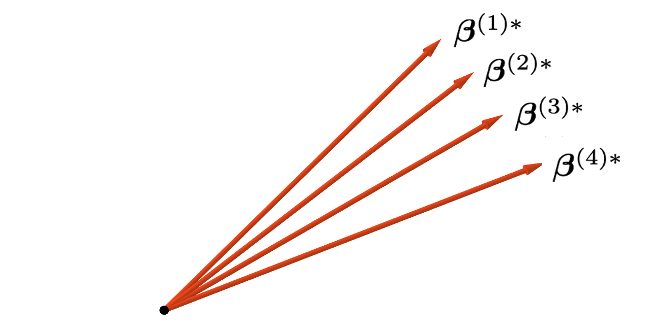
(a) Distance-based similarity (Bastani, 2021; Duan and Wang, 2022; Li et al., 2022b; Tian and Feng, 2022)

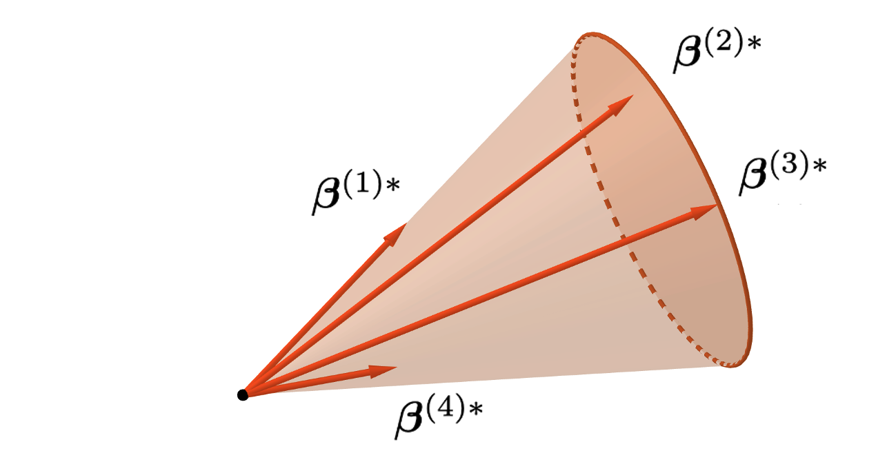
(b) Angle-based similarity (Gu et al., 2022)
                                                                                                                                                 
                                                                                                                                                 

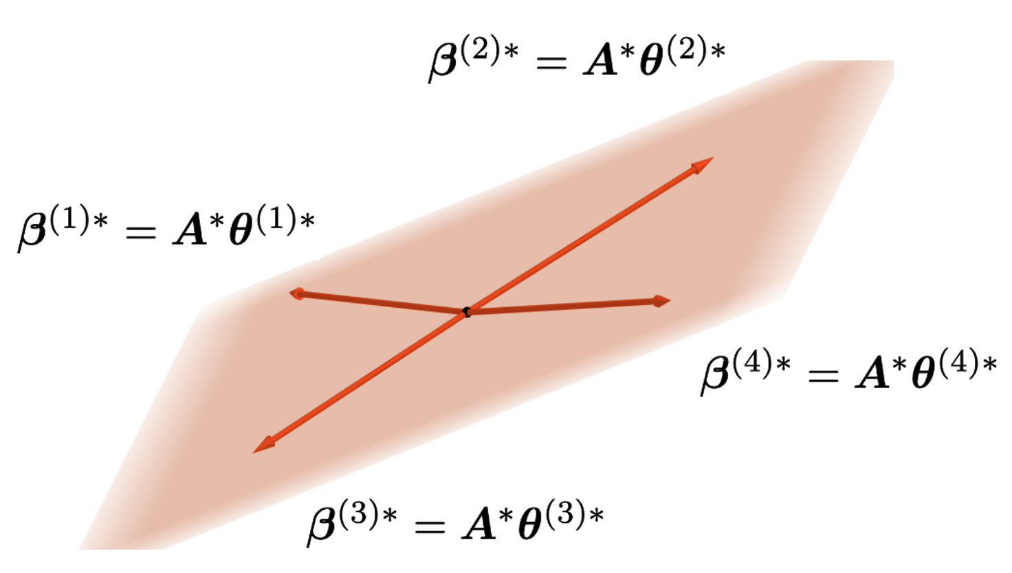
(c) The same representation (Du et al., 2020; Tripuraneni et al., 2021)

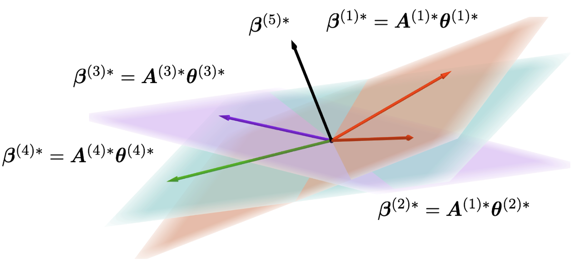
(d) Similar representations with outliers (ours)
                                                                                                                                                 

Figure 1: A simple visualization of four different settings under linear model (1).

1.2 Our Contributions

Our contributions can be summarized below.

1. Compared to most of the literature on representation MTL and TL, we considered a more general framework, where the linear representations can differ across tasks, and there can be a few unknown outlier tasks.

2. We proposed two-step algorithms to learn the regression coefficients and the representations from multiple tasks (MTL problem), and the shared information can be leveraged to learn a new target task (TL problem). Our algorithms were shown to have the following properties:

   • Outperform the single-task and target-only learning when the representations of different tasks are sufficiently similar and the fraction of outlier tasks is small.

   • Always perform no worse than single-task and target-only learning (safe-net guarantee), even when the representations across tasks are dissimilar.

   The upper bounds we obtained are better than the rates presented in Chua et al. (2021) and Duan and Wang (2022). They do not consider the case of outlier tasks.

3. We derived the lower bounds for model (1) for MTL and TL problems. To the best of our knowledge, these are the first lower bound results for regression coefficient estimation under the representation MTL and TL settings. Duchi et al. (2022) and Tripuraneni et al. (2021) provided similar lower bounds for the subspace recovery problem when all representations are the same without outlier tasks. Chua et al. (2021) showed that assuming the same representation can lead to worse performance than target-only learning when source representations differ from each other, but they did not provide a full lower bound which relates to the representation difference. Comparing the upper and lower bounds, we showed that our algorithms are nearly minimax optimal in a large regime.

4. We extended our analysis from linear model (1) to generalized linear models (GLMs) and non-linear regression models, and obtained similar theoretical guarantees in these settings.

5. We proposed an algorithm based on SVD to make it adaptive to an unknown intrinsic dimension $r$. In almost all prior works, $r$ is assumed to be known as a priori, which is usually not the case in practice.

1.3 Notations and Organization

Throughout the paper, we use bold capitalized and lower-case letters to denote matrices and vectors, respectively. For a vector $\bm{u}$, $\|\bm{u}\|_{2}$ stands for its Euclidean norm. For a matrix $\bm{A}$, $\|\bm{A}\|_{2}$ and $\|\bm{A}\|_{\textup{F}}$ represent its spectral and Frobenius norm, respectively. $\bm{A}^{T}$ denotes its transpose, where the operator $T$ should not be confused with the number of tasks $T$. For a real number $a$, $|a|$ stands for its absolute value. $\sigma_{j}(\bm{A})$, $\sigma_{\max}(\bm{A})$, $\sigma_{\min}(\bm{A})$ are its $j$-th largest singular value, maximum singular value, and minimum singular value, respectively. When $\bm{A}$ is a square matrix, we denote its maximum and minimum eigenvalues as $\lambda_{\max}(\bm{A})$ and $\lambda_{\min}(\bm{A})$, respectively. For a function $\psi:\mathcal{X}\rightarrow\mathbb{R}$, $\|\psi\|_{\infty}$ is defined to be $\max_{x\in\mathcal{X}}|\psi(x)|$. For two real numbers $a$ and $b$, we denote their minimum by $\min\{a,b\}$ or $a\wedge b$ and their maximum by $\max\{a,b\}$ or $a\vee b$, respectively. For two positive real sequences $\{a_{n}\}_{n=1}^{\infty}$ and $\{b_{n}\}_{n=1}^{\infty}$, $a_{n}\lesssim b_{n}$ or $b_{n}\gtrsim a_{n}$ means there exists a universal constant $C>0$ such that $a_{n}\leq Cb_{n}$ for all $n$, and $a_{n}\ll b_{n}$ or $b_{n}\gg a_{n}$ means that $a_{n}/b_{n}\rightarrow 0$ as $n\rightarrow\infty$. $a_{n}\asymp b_{n}$ means $a_{n}\lesssim b_{n}$ and $a_{n}\gtrsim b_{n}$ hold simultaneously. Sometimes we abbreviate “with probability” as “w.p.” and “with respect to” as “w.r.t.”. For any $N\in\mathbb{N}_{+}$, $[N]$ and $1:N$ are defined to be $\{1,\ldots,N\}$. $\mathbb{P}$ and $\mathbb{E}$ are the probability measure and expectation taken over all randomness. We use $C,C^{\prime},C^{\prime\prime},C_{1},C_{2},C_{3},c,c^{\prime}$ to represent universal constants that could change from place to place.

The rest of this paper is organized as follows. In Section 2, we proposed a two-step learning algorithm for linear model (1) under the MTL setting, and established the corresponding upper and lower bounds. In Section 3, we studied how to transfer the knowledge to an unknown task, i.e., under the setting of TL or learning-to-learn. We proposed another two-step algorithm that takes the MTL algorithm’s output as input and adapts it to the new target task. The corresponding upper and lower bounds were presented. Moreover, we extended the linear model (1) to generalized linear models (GLMs) and non-linear regression models in Section 4. In Section 5, we proposed an extension to make the MTL and TL algorithms adaptive to the case where the intrinsic dimension $r$ is unknown. Finally, we summarized our contributions and discussed a few future research avenues in Section 7. All the proofs can be found in Appendix.

2 Multi-task Learning with Similar Representations

2.1 Problem Set-up

We describe the model introduced in Section 1 in more detail. Suppose there are $T$ tasks, and we have collected sample $\{\bm{x}^{(t)}_{i},y^{(t)}_{i}\}_{i=1}^{n}$ from the $t$-th task, where $\bm{x}^{(t)}_{i}\in\mathbb{R}^{p}$, $y^{(t)}_{i}\in\mathbb{R}$, and $t\in[T]$. There exists an unknown subset $S\subseteq[T]$, such that for all $t\in S$,

$$y^{(t)}_{i}=(\bm{x}^{(t)}_{i})^{T}\bm{\beta}^{(t)*}+\epsilon^{(t)}_{i},\quad i=1:n,$$ (2)

where $\bm{\beta}^{(t)*}=\bm{A}^{(t)*}\bm{\theta}^{(t)*}$, $\bm{A}^{(t)*}\in\mathcal{O}^{p\times r}=\{\bm{A}\in\mathbb{R}^{p\times r}:\bm{A}^{T}\bm{A}=\bm{I}_{r}\}$, low-dimensional parameter $\bm{\theta}^{(t)*}\in\mathbb{R}^{r}$, $r\leq p$, and $\{\epsilon^{(t)}_{i}\}_{i=1}^{n}$ are i.i.d. zero-mean sub-Gaussian variables independent of $\{\bm{x}^{(t)}_{i}\}_{i=1}^{n}$ . Throughout this section, we assume the intrinsic dimension $r$ is known. The case that $r$ is unknown will be dealt with in Section 5.

Here $T$ tasks are divided into two parts, $S$ and $S^{c}$. The tasks in $S$ have “similar” representations (similarity to be defined in the following), while the tasks in $S^{c}$ can be understood as outlier tasks or contaminated tasks, which can be arbitrarily distributed. Our goal is two folds:

1. Improve the learning performance simultaneously on the tasks in $S$, when they share “similar” representations and the number of outlier tasks in $S^{c}$ is small;

2. Maintain the single-task learning performance when the “similarity” between tasks in $S$ is low.

It should be emphasized that if we allow the outlier tasks in $S^{c}$ to be arbitrarily distributed, no guarantee can be obtained for these tasks in the worst case. However, as we will see, if these tasks still follow linear models (2) (without a low-dimensional representation), then we can achieve the single-task linear regression estimation rate on $\{\bm{\beta}^{(t)*}\}_{t\in S^{c}}$.

We also want to point out that the set $S$ is unknown. We will show that our learning algorithms can perform well in all the cases of $S\subseteq[T]$ under certain conditions. This can be understood from two different perspectives. From the perspective of outlier tasks, we expect an algorithm to succeed for all possible outlier task index sets $S^{c}$ as long as $|S^{c}|$ is small. In other words, the algorithm should not only work for a specific $S^{c}$ and it should not rely on the indices of tasks (Otherwise, we can always drop the data from tasks in $S^{c}$ to avoid the impact of outliers). Another perspective is from the adversarial attacks. The attacker can choose to corrupt the data from any task, which usually happens after the release of the machine learning system. Therefore, a robust learner should achieve ideal performance for all cases of $S$. See Figure 2 for an illustration of these two points of view.

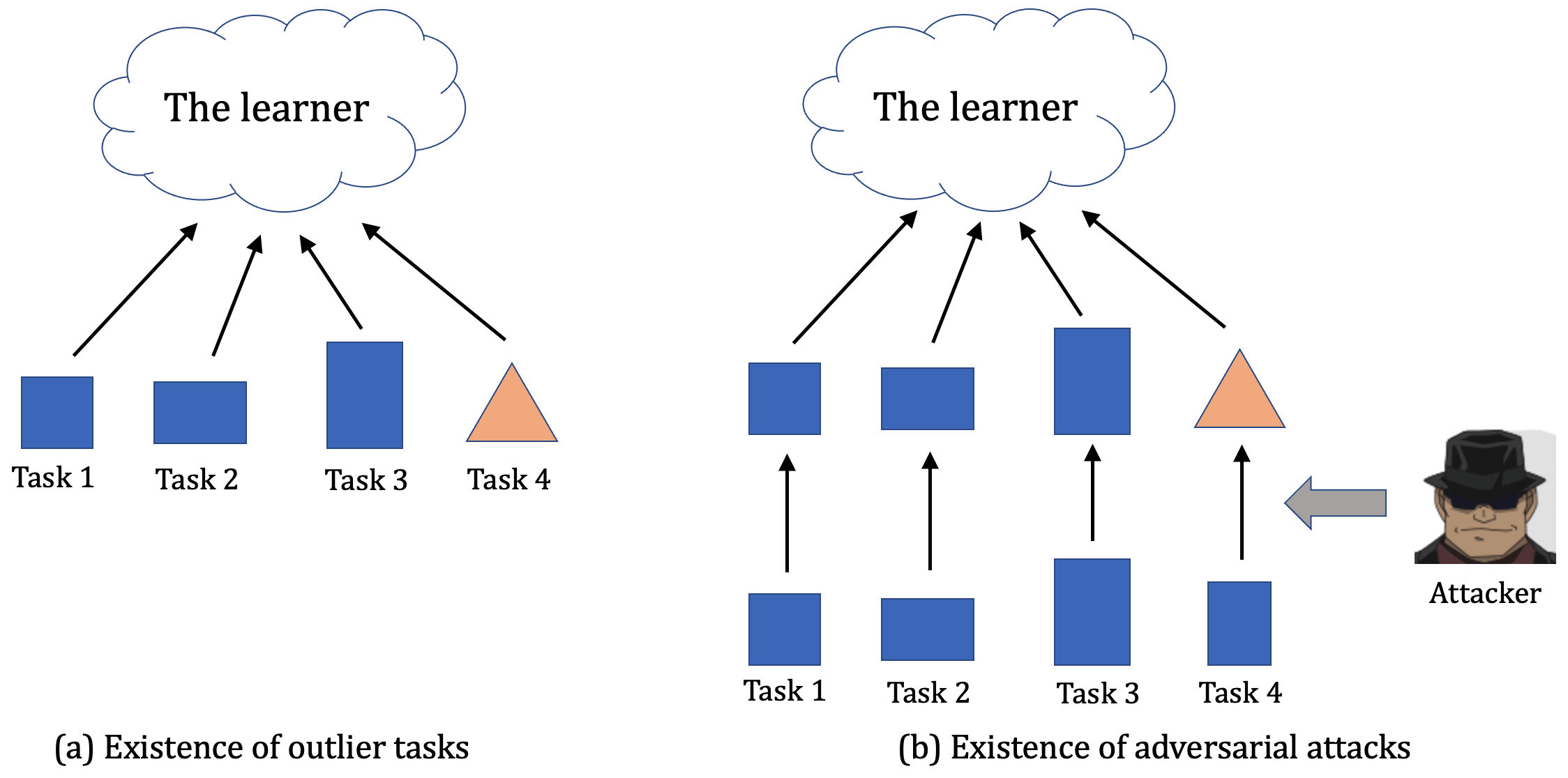
Figure 2: An illustration for two perspectives of viewing model (2). In both cases, $S^{c}=\{4\}$.

The same setting when $\bm{A}^{(t)*}$’s are the same and $S=[T]$ (i.e. no outlier tasks) has been studied in Du et al. (2020), where they argued that when $r$ is much smaller than $p$, a better estimation error rate of $\bm{\beta}^{(t)*}$ can be achieved compared to the single-task learning. Our framework is more general and closer to the practical situation because it is difficult for all tasks to be embedded in precisely the same subspace as the number of tasks $T$ grows (Rostami et al., 2022), and the issue of outlier tasks is also very common (Zhang and Yang, 2018).

To mathematically describe the similarity between representations $\{\bm{A}^{(t)*}\}_{t\in S}$, we consider the maximum principal angle between subspaces spanned by the columns of these representation matrices. More specifically, we assume that there exists $h\in[0,1]$ , such that

$$\min_{\macc@depth\char 1\relax\frozen@everymath{\macc@group}\macc@set@skewchar\macc@nested@a 111{}\in\mathcal{O}^{p\times r}}\max_{t\in S}\|\bm{A}^{(t)*}(\bm{A}^{(t)*})^{T}-\macc@depth\char 1\relax\frozen@everymath{\macc@group}\macc@set@skewchar\macc@nested@a 111{}(\macc@depth\char 1\relax\frozen@everymath{\macc@group}\macc@set@skewchar\macc@nested@a 111{})^{T}\|_{2}\leq h.$$ (3)

A small $h$ means the representations are more similar. The case when $h=0$ reduces to the setting of the same representations in literature (Du et al., 2020; Tripuraneni et al., 2021). The case when $r=1$ (where all representations are $p\times 1$ vectors and $\bm{\theta}^{(t)*}$’s are scalars) reduces to the setting of Gu et al. (2022). In this case, the principle angle between subspaces becomes the angle between regression cofficient vectors.

We now make some assumptions. Without loss of generality, suppose $\bm{x}^{(t)}$ is mean-zero. Denote the covariance matrix $\bm{\Sigma}^{(t)}=\mathbb{E}[\bm{x}^{(t)}(\bm{x}^{(t)})^{T}]$ and the joint distribution of $\{\{\bm{x}^{(t)}_{i},y^{(t)}_{i}\}_{i=1}^{n}\}_{t\in S^{c}}$ as $\mathbb{Q}_{S^{c}}$. For the convenience of description, define a coefficient matrix $\bm{B}_{S}^{*}\in\mathbb{R}^{p\times|S|}$, each column of which is a coefficient vector in $\{\bm{\beta}^{(t)*}\}_{t\in S}$.

Assumption 1

For any $t\in S$, $\bm{x}^{(t)}$ is sub-Gaussian in the sense that for any $\bm{u}\in\mathbb{R}^{p}$ and $\lambda\in\mathbb{R}$, $\mathbb{E}[e^{\lambda\bm{u}^{T}\bm{x}^{(t)}}]\leq e^{C\lambda^{2}\|\bm{u}\|_{2}^{2}}$ with some constant $C>0$. And there exist constants $c,C$ such that $0<c\leq\lambda_{\min}(\bm{\Sigma}^{(t)})\leq\lambda_{\max}(\bm{\Sigma}^{(t)})\leq C<\infty$, for all $t\in S$.

Assumption 2

There exist constants $c,C$ such that $\max_{t\in S}\|\bm{\theta}^{(t)*}\|_{2}\leq C<\infty$ and $\sigma_{r}(\bm{B}_{S}^{*}/\allowbreak\sqrt{|S|})\geq\frac{c}{\sqrt{r}}$, where each column of $\bm{B}_{S}^{*}$ is a coefficient vector in $\{\bm{\beta}^{(t)*}\}_{t\in S}$.

Assumption 3

$n\geq C(p+\log T)$ with a sufficiently large constant $C>0$.

Assumptions 1 and 3 are standard conditions in literature (Du et al., 2020; Duan and Wang, 2022). The second part of Assumption 2 related to $\sigma_{r}(\bm{B}_{S}^{*}/\sqrt{|S|})$ is often called the task diversity condition. When $\bm{A}^{(t)*}$’s are the same, $\sigma_{r}(\bm{B}_{S}^{*}/\sqrt{|S|})=\sigma_{r}(\bm{\Theta}^{*}_{S}/\sqrt{|S|})$, where each column of $\bm{\Theta}^{*}_{S}$ is a coefficient vector in $\{\bm{\theta}^{(t)}\}_{t\in S}$, which means that the low-dimensional task-specific parameters $\bm{\theta}^{(t)*}$’s are diverse. Such a task diversity condition has been adopted in other related literature (Chua et al., 2021; Du et al., 2020; Duchi et al., 2022; Tripuraneni et al., 2021) , to obtain a parametric rate which is faster than the rate without this condition (Maurer et al., 2016). The benefit of this condition is intuitive to understand, because a full exploration of all directions in the subspace is necessary to learn representations well, which is the key in representation MTL and TL.

It is important to note that the presented assumptions are imposed on both the set of outlier tasks $S^{c}$ and the model parameters. These assumptions are made from the perspective of outlier tasks. However, when considering adversarial attacks, we can replace $S$ with the set of all tasks $[T]$ and assume that each task follows the linear model (2). An attacker can then adversarially select a subset $S^{c}\subseteq[T]$ and distort the data distribution for these tasks. For simplicity, we do not distinguish between these two perspectives in the following parts of this paper.

In the following subsection, we will present an algorithm to achieve our proposed two goals and provide the associated upper bounds of the estimation error.

2.2 Upper Bounds

In a special case of our setting, when $\bm{A}^{(t)*}$’s are the same and $S=[T]$, Du et al. (2020) proposed an algorithm by combining the objective functions of all tasks and solving the optimization problem. A more general version of it for general loss functions has been explored in Tripuraneni et al. (2020). Under our setting, where the representations are similar but not exactly the same and with potential outlier tasks, the objective function needs to be properly adjusted. When $h$ is large, learning $\{\bm{\beta}^{(t)*}\}_{t\in S}$ by presuming similar representations may lead to a negative transfer effect. Considering these differences, we proposed a two-step learning approach in Algorithm 1 that addresses these issues. Note that we will apply the same algorithm to some extended models in Section 4, so for description convenience, we introduce the algorithm with generic loss functions $f^{(t)}$ for the $t$-th task. For linear model (2), we set $f^{(t)}(\bm{\beta})=\frac{1}{n}\|\bm{Y}^{(t)}-\bm{X}^{(t)}\bm{\beta}\|_{2}=\frac{1}{n}\sum_{i=1}^{n}[y^{(t)}_{i}-(\bm{x}^{(t)}_{i})^{T}\bm{\beta}]^{2}$ for $\bm{\beta}\in\mathbb{R}^{p}$, where $\bm{X}^{(t)}\in\mathbb{R}^{n\times p}$ and $\bm{Y}^{(t)}\in\mathbb{R}^{n}$ are corresponding matrix representations of the data from the $t$-th task.

Input: Data $\{\bm{X}^{(t)},\bm{Y}^{(t)}\}_{t=1}^{T}=\{\{\bm{x}^{(t)}_{i},y^{(t)}_{i}\}_{i=1}^{n}\}_{t=1}^{T}$, penalty parameters $\lambda$ and $\gamma$

Output: Estimators $\{\widehat{\bm{\beta}}^{(t)}\}_{t=1}^{T},\widehat{\macc@depth\char 1\relax\frozen@everymath{\macc@group}\macc@set@skewchar\macc@nested@a 111{}}$

1 Step 1: $\{\widehat{\bm{A}}^{(t)}\}_{t=1}^{T}$, $\{\widehat{\bm{\theta}}^{(t)}\}_{t=1}^{T}$, $\widehat{\macc@depth\char 1\relax\frozen@everymath{\macc@group}\macc@set@skewchar\macc@nested@a 111{}}\in$ $\operatorname*{arg\,min}_{\{\bm{A}^{(t)}\}_{t=1}^{T},\{\bm{\theta}^{(t)}\}_{t=1}^{T},\macc@depth\char 1\relax\frozen@everymath{\macc@group}\macc@set@skewchar\macc@nested@a 111{}}\big{\{}\frac{1}{T}\big{[}\sum_{t=1}^{T}f^{(t)}(\bm{A}^{(t)}\bm{\theta}^{(t)})+\frac{\lambda}{\sqrt{n}}\|\bm{A}^{(t)}(\bm{A}^{(t)})^{T}-\macc@depth\char 1\relax\frozen@everymath{\macc@group}\macc@set@skewchar\macc@nested@a 111{}(\macc@depth\char 1\relax\frozen@everymath{\macc@group}\macc@set@skewchar\macc@nested@a 111{})^{T}\|_{2}\big{]}\big{\}}$

Step 2: $\widehat{\bm{\beta}}^{(t)}=\operatorname*{arg\,min}_{\bm{\beta}\in\mathbb{R}^{p}}\big{\{}f^{(t)}(\bm{\beta})+\frac{\gamma}{\sqrt{n}}\|\bm{\beta}-\widehat{\bm{A}}^{(t)}\widehat{\bm{\theta}}^{(t)}\|_{2}\big{\}}$ for $t\in[T]$

Algorithm 1 Representation multi-task learning (RL-MTL)

In Algorithm 1, Step 1 aims to learn all tasks by aggregating the data, where the penalty $\|\bm{A}^{(t)}(\bm{A}^{(t)})^{T}-\macc@depth\char 1\relax\frozen@everymath{\macc@group}\macc@set@skewchar\macc@nested@a 111{}(\macc@depth\char 1\relax\frozen@everymath{\macc@group}\macc@set@skewchar\macc@nested@a 111{})^{T}\|_{2}$ is added to force the subspaces represented by $\{\widehat{\bm{A}}^{(t)}\}_{t=1}^{T}$ to be similar. This penalty form is motivated by Duan and Wang (2022), where a similar penalty is applied on regression coefficient vectors. Note that when $\|\bm{A}^{(t)}(\bm{A}^{(t)})^{T}-\macc@depth\char 1\relax\frozen@everymath{\macc@group}\macc@set@skewchar\macc@nested@a 111{}(\macc@depth\char 1\relax\frozen@everymath{\macc@group}\macc@set@skewchar\macc@nested@a 111{})^{T}\|_{2}=0$, it can be shown that $\bm{A}^{(t)}$ and $\macc@depth\char 1\relax\frozen@everymath{\macc@group}\macc@set@skewchar\macc@nested@a 111{}$ are identical up to a rotation. And this distance is equivalent to other subspace distances like $\sin$-$\Theta$ distance or the distance between two matrices up to a rotation (Chen et al., 2021b). Step 2 uses data from each task to make potential corrections to prevent negative transfer. Such two-step methods are commonly used in the distance-based MTL and TL literature to reduce the impact of negative transfer (Bastani, 2021; Li et al., 2022b; Lin and Reimherr, 2022; Tian and Feng, 2022). It is important to point out that $\bm{A}^{(t)*}$’s and $\bm{\theta}^{(t)*}$’s are not uniquely identifiable in model (2), which is not a problem because our focus is the estimation of $\bm{\beta}^{(t)*}$’s.

Next, we present the upper bound of estimation errors of $\{\bm{\beta}^{(t)*}\}_{t\in S}$ incurred by Algorithm 1.

Theorem 1 (Upper bound for MTL)

Suppose Assumptions 1-3 hold. By setting $\lambda=C\sqrt{r(p+\log T)}$ and $\gamma=C^{\prime}\sqrt{p+\log T}$ with sufficiently large positive constants $C$ and $C^{\prime}$, w.p. at least $1-e^{-C^{\prime\prime}(r+\log T)}$, for all $S\subseteq[T]$ satisfying $\frac{|S^{c}|}{T}r^{3/2}\leq$ a small constant $c$ and an arbitrary distribution $\mathbb{Q}_{S^{c}}$ of $\{\{\bm{x}^{(t)}_{i},y^{(t)}_{i}\}_{i=1}^{n}\}_{t\in S^{c}}$, we have

$$\max_{t\in S}\|\widehat{\bm{\beta}}^{(t)}-\bm{\beta}^{(t)*}\|_{2}\lesssim\left(r\sqrt{\frac{p}{nT}}+\sqrt{r}h+\sqrt{r}\sqrt{\frac{r+\log T}{n}}+\sqrt{\frac{p}{n}}\cdot\frac{|S^{c}|}{T}r^{3/2}\right)\wedge\sqrt{\frac{p+\log T}{n}}.$$ (4)

Furthermore, if the data from tasks in $S^{c}$ satisfies the linear model (2) (without any latent structure assumption) and Assumption 1, then w.p. at least $1-e^{-C^{\prime}(p+\log T)}$, we also have

$$\max_{t\in[T]}\|\widehat{\bm{\beta}}^{(t)}-\bm{\beta}^{(t)*}\|_{2}\lesssim\sqrt{\frac{p+\log T}{n}}.$$ (5)

Remark 2

The upper bound of $\max_{t\in S}\|\widehat{\bm{\beta}}^{(t)}-\bm{\beta}^{(t)*}\|_{2}$ is the minimum of two terms, where the first term corresponds to the rate obtained through data aggregation and the second term corresponds to the single task rate. It shows that our algorithm is automatically adaptive to the optimal situation, no matter whether learning through data aggregation is beneficial or not. Furthermore, it is robust to a small fraction of outlier tasks, in the sense that representation MTL is still beneficial when the outlier fraction $|S^{c}|/T$ is small.

Remark 3

On the other hand, the upper bound of $\max_{t\in S}\|\widehat{\bm{\beta}}^{(t)}-\bm{\beta}^{(t)*}\|_{2}$ consists of a few components. Rate $r\sqrt{\frac{p}{nT}}+\sqrt{r}h$ is due to learning similar representations, $\sqrt{r}\sqrt{\frac{r+\log T}{n}}$ is due to learning the representations and task-specific parameters, $\sqrt{\frac{p}{n}}\frac{|S^{c}|}{T}r^{3/2}$ is caused by outlier tasks, and $\sqrt{\frac{p+\log T}{n}}$ is the single-task learning rate. When $T\gg r^{2}$ (a large number of tasks), $h\ll\sqrt{\frac{p+\log T}{nr}}$ (similar representations), $p\gg r(r\vee\log T)$ (a low intrinsic dimension), and $\frac{|S^{c}|}{T}r^{3/2}\ll 1$ (a small number of outlier tasks), the rate is faster than the single-task learning rate $\sqrt{\frac{p+\log T}{n}}$.

Remark 4

When $h=0$ and $S=[T]$, our upper bound of $\max_{t\in S}\|\widehat{\bm{\beta}}^{(t)}-\bm{\beta}^{(t)*}\|_{2}$ reduces to $\big{(}r\sqrt{\frac{p}{nT}}+\sqrt{r}\sqrt{\frac{r+\log T}{n}}\big{)}\wedge\sqrt{\frac{p+\log T}{n}}$, which matches the rate in Du et al. (2020). When $S=[T]$, we can adapt our setting to that of Duan and Wang (2022) to compare the results. Duan and Wang (2022) assumes $\bm{\beta}^{(t)*}=\bm{A}^{*}\bm{\theta}^{(t)*}+\bm{\delta}^{(t)*}$ with some $\bm{A}^{*}\in\mathcal{O}^{p\times r}$ and $\|\bm{\delta}^{(t)*}\|_{2}\leq\delta/\sqrt{n}$. It is not hard to show that when $\delta\asymp\sqrt{n}h$, our setting and theirs are in the same regime. Then the upper bound in Theorem 1 is strictly better than the upper bound in Theorem 4.6 in their paper, in terms of a better dependence on $r$ and a weaker condition on $n$ (They require $n\gtrsim r(p+\log T)\log n\log T$).

As we pointed out in Section 1.1, our setting reduces to the setting in Gu et al. (2022) when $r=1$, where they considered a ridge regression by penalizing the angle between different regression coefficients. The main idea of our Algorithm 1 resembles their approach, but they only considered the case when the angles between different regression coefficients are in $[0,\pi/2]$. Our result shows that multi-task learning helps as long as the subspaces spanned by each coefficient (i.e., the straight line) are similar, where the angles can be either close to $0$ or $\pi$. Moreover, surprisingly, it turns out that when $r=1$, the estimators obtained from Step 1 of Algorithm 1 already achieve the desired rate, which means we can drop Step 2. The detailed results are as follows.

Theorem 5 (No need for Step 2 when $r=1$)

Consider the case that $r=1$. Under the same assumptions imposed in Theorem 1, w.p. at least $1-e^{-C^{\prime}(1+\log T)}$, for all $S\subseteq[T]$ satisfying $\frac{|S^{c}|}{T}\leq$ a small constant $c$ and an arbitrary distribution $\mathbb{Q}_{S^{c}}$ of $\{\{\bm{x}^{(t)}_{i},y^{(t)}_{i}\}_{i=1}^{n}\}_{t\in S^{c}}$, we have

$$\max_{t\in S}\|\widehat{\bm{A}}^{(t)}\widehat{\bm{\theta}}^{(t)}-\bm{\beta}^{(t)*}\|_{2}\lesssim\left(\sqrt{\frac{p}{nT}}+h+\sqrt{\frac{1+\log T}{n}}+\sqrt{\frac{p}{n}}\cdot\frac{|S^{c}|}{T}\right)\wedge\sqrt{\frac{p+\log T}{n}}.$$ (6)

Furthermore, if we assume the data from tasks in $S^{c}$ satisfies the linear model (2) (without any latent structure assumption) and Assumption 1, then w.p. at least $1-e^{-C^{\prime}(p+\log T)}$, we also have

$$\max_{t\in[T]}\|\widehat{\bm{A}}^{(t)}\widehat{\bm{\theta}}^{(t)}-\bm{\beta}^{(t)*}\|_{2}\lesssim\sqrt{\frac{p+\log T}{n}}.$$ (7)

Remark 6

Note that when $r=1$, the task diversity condition in Assumption 2, i.e. $\sigma_{1}(\bm{B}^{*}_{S}/\sqrt{|S|})\geq c$, holds automatically when $\min_{t\in S}\|\bm{\theta}^{(t)*}\|_{2}\geq c>0$.

2.3 Lower Bounds

In this subsection, we construct the lower bounds to explore the information-theoretic hardness of the representation MTL problem. Consider the space for all subsets $S\subseteq[T]$ as

$$\mathcal{S}=\{S\subseteq[T]:|S^{c}|/T\leq\epsilon\}.$$ (8)

Given the subset $S$, define a coefficient matrix $\bm{B}_{S}\in\mathbb{R}^{p\times|S|}$, each column of which corresponds to a coefficient vector in $\{\bm{\beta}^{(t)}\}_{t\in S}$. Consider the parameter spaces for the coefficient vectors $\{\bm{\beta}^{(t)}\}_{t\in S}$ as

$$\mathscr{B}(S,h)= \bigg{\{}\{\bm{\beta}^{(t)}\}_{t\in S}:\bm{\beta}^{(t)}=\bm{A}^{(t)}\bm{\theta}^{(t)}\text{ for all }t\in S,\{\bm{A}^{(t)}\}_{t\in S}\subseteq\mathcal{O}^{p\times r},\max_{t\in S}\|\bm{\theta}^{(t)}\|_{2}\leq C,$$ (9)

$$\min_{\macc@depth\char 1\relax\frozen@everymath{\macc@group}\macc@set@skewchar\macc@nested@a 111{}\in\mathcal{O}^{p\times r}}\max_{t\in S}\|\bm{A}^{(t)}(\bm{A}^{(t)})^{T}-\macc@depth\char 1\relax\frozen@everymath{\macc@group}\macc@set@skewchar\macc@nested@a 111{}{\macc@depth\char 1\relax\frozen@everymath{\macc@group}\macc@set@skewchar\macc@nested@a 111{}}^{T}\|_{2}\leq h,\sigma_{r}\Big{(}|S|^{-1/2}\bm{B}_{S}\Big{)}\geq\frac{c}{\sqrt{r}}\bigg{\}}$$ (10)

where $C$ and $c$ can be any fixed positive constants such that $\mathscr{B}(S,h)\neq\emptyset$. We have the following lower bound.

Theorem 7 (Lower bound for MTL)

Suppose $p\geq 2r$ and $\epsilon\leq c/r$ where $c$ is a small constant. We have the following lower bound hold:

$$\inf_{\{\widehat{\bm{\beta}}^{(t)}\}_{t=1}^{T}}\sup_{S\subseteq\mathcal{S}}\sup_{\begin{subarray}{c}\{\bm{\beta}^{(t)}\}_{t\in S}\in\mathscr{B}(S,h)\\ \mathbb{Q}_{S^{c}}\end{subarray}}\mathbb{P}\bigg{(}\max_{t\in S}\|\widehat{\bm{\beta}}^{(t)}-\bm{\beta}^{(t)*}\|_{2}\gtrsim\sqrt{\frac{pr}{nT}}+\sqrt{\frac{r+\log T}{n}}+h\wedge\sqrt{\frac{p+\log T}{n}}+\frac{\epsilon r}{\sqrt{n}}\bigg{)}\geq\frac{1}{10},$$ (11)

where for any given $S\subseteq\mathcal{S}$, $\mathbb{P}=\mathbb{P}_{S}\otimes\mathbb{Q}_{S^{c}}$, and $\mathbb{P}_{S}$, $\mathbb{Q}_{S^{c}}$ are the probability measures on sample space of tasks in $S$, $S^{c}$, respectively. Furthermore, if tasks in $S^{c}$ also follow the linear model (2), then we have the following lower bound, where $\mathbb{P}$ is the probability measure on sample space of all tasks:

$$\inf_{\{\widehat{\bm{\beta}}^{(t)}\}_{t=1}^{T}}\sup_{S\subseteq\mathcal{S}}\sup_{\begin{subarray}{c}\{\bm{\beta}^{(t)}\}_{t\in S}\in\mathscr{B}(S,h)\\ \{\bm{\beta}^{(t)}\}_{t\in S^{c}}\end{subarray}}\mathbb{P}\bigg{(}\max_{t\in[T]}\|\widehat{\bm{\beta}}^{(t)}-\bm{\beta}^{(t)*}\|_{2}\gtrsim\sqrt{\frac{p+\log T}{n}}\bigg{)}\geq\frac{1}{10}.$$ (12)

Remark 8

Similar to the upper bound in Theorem 1, the lower bound of $\max_{t\in S}\|\widehat{\bm{\beta}}^{(t)}-\bm{\beta}^{(t)*}\|_{2}$ contains a few terms which reflect the hardness of learning different components. For example, $\sqrt{\frac{pr}{nT}}+h\wedge\sqrt{\frac{p+\log T}{n}}$ is due to learning the similar representations in $S$, $\sqrt{\frac{r+\log T}{n}}$ is due to learning the task-specific parameters, and $\frac{\epsilon r}{\sqrt{n}}$ is due to outlier tasks.

To our knowledge, this is the first lower bound for learning regression parameters in the context of multi-task representation learning. Tripuraneni et al. (2021) and Duchi et al. (2022) gave lower bounds for the subspace recovery under a similar setting, where there are no outlier tasks and all tasks share the same representations. Comparing the upper and lower bounds, we can see that the dependence on $r$ in the upper bound is not optimal. A similar phenomenon has been noticed in Tripuraneni et al. (2021), where they proposed an empirical risk minimization estimator and a method-of-moment estimator. The upper bounds of estimation errors for both estimators have sub-optimal dependence on $r$ under our Assumption 2. They correlated this to a similar phenomenon observed in other works on linear regression models (Raskutti et al., 2011), where the upper bounds of estimation errors have sub-optimal dependence on eigenvalues of design matrices. In addition, the last term in our lower bound $\frac{\epsilon r}{\sqrt{n}}$ does not depend on the dimension $p$, while the counterpart in the upper bound does. A similar phenomenon has been noted in multiple papers (Duan and Wang, 2022; Tian et al., 2022). As pointed out in Tian et al. (2022), estimators based on techniques in robust statistics like Tukey’s depth function have been shown to achieve minimax rate under Huber’s contamination model for location and covariance estimation (Chen et al., 2018), which might be helpful to improve the upper bound in our setting as well.

When $r$ is bounded and $\epsilon=0$, the upper and lower bounds match. Note that it is often reasonable for $r$ to be bounded since it captures the intrinsic dimension of the problem. And $\epsilon=0$ implies no outlier tasks. An adaptation of techniques in robust statistics to improve our estimation algorithm will be an interesting future research direction.

3 Transferring to New Tasks (Learning-to-learn)

3.1 Problem Set-up

In this section, in addition to data from the $T$ tasks, suppose we also observe data $\{(\bm{x}^{(0)}_{i},y^{(0)}_{i})\}_{i=1}^{n_{0}}$ from a new task

$$y^{(0)}_{i}=(\bm{x}^{(0)}_{i})^{T}\bm{\beta}^{(0)*}+\epsilon^{(0)}_{i},\quad i=1:n_{0},$$ (13)

where $\bm{\beta}^{(0)*}=\bm{A}^{(0)*}\bm{\theta}^{(0)*}$, $\bm{A}^{(0)*}\in\mathcal{O}^{p\times r}=\{\bm{A}\in\mathbb{R}^{p\times r}:\bm{A}^{T}\bm{A}=\bm{I}_{r}\}$, $\bm{\theta}^{(0)*}\in\mathbb{R}^{r}$, and $\{\epsilon^{(0)}_{i}\}_{i=1}^{n_{0}}$ are i.i.d. zero-mean sub-Gaussian variables independent of $\{\bm{x}^{(0)}_{i}\}_{i=1}^{n_{0}}$. Similar to Section 2, the intrinsic dimension $r$ is assumed to be known, and we leave the case of unknown $r$ to Section 5. Under such a transfer learning (TL) or learning-to-learn setting, the new task is often called the target task, and the $T$ tasks are called source tasks. Our goal is two-fold:

1. Transfer knowledge from source tasks to improve the learning performance on the target task, when the source and target share “similar” representations and the number of outlier source tasks is small;

2. Ensure the learning performance is no worse than the target-only learning performance to avoid the negative transfer.

To describe the similarity between target and source representations, we assume

$$\max_{t\in S}\|\bm{A}^{(t)*}(\bm{A}^{(t)*})^{T}-\bm{A}^{(0)*}(\bm{A}^{(0)*})^{T}\|_{2}\leq h,$$ (14)

where $S$ is a subset of $[T]$. Similar to the setting in the last section, the joint distribution $\mathbb{Q}_{S^{c}}$ of data from source tasks in $S^{c}$, i.e., $\{\{\bm{x}^{(t)}_{i},y^{(t)}_{i}\}_{i=1}^{n}\}_{t\in S^{c}}$, is allowed to be arbitrary. Denote $\bm{\Sigma}^{(0)}=\mathbb{E}[\bm{x}^{(0)}(\bm{x}^{(0)})^{T}]$. We impose the following assumptions on the target task.

Assumption 4

For $\bm{u}\in\mathbb{R}^{p}$, $\bm{u}^{T}\bm{x}^{(0)}$ is sub-Gaussian in the sense that $\mathbb{E}[e^{\lambda\bm{u}^{T}\bm{x}^{(0)}}]\leq e^{C\lambda^{2}\|\bm{u}\|_{2}^{2}}$ for any $\lambda\in\mathbb{R}$ with some constant $C>0$. And there exist constants $c,C$ such that $0<c\leq\lambda_{\min}(\bm{\Sigma}^{(0)})\leq\lambda_{\max}(\bm{\Sigma}^{(0)})\leq C<\infty$.

Assumption 5

There exists a constant $C>0$ such that $\|\bm{\theta}^{(0)*}\|_{2}\leq C<\infty$.

Assumption 6

$n_{0}\geq Cp$ with a sufficiently large constant $C>0$.

Remark 9

Assumption 6 is imposed to guarantee the target-only rate $\sqrt{p/n_{0}}$. If we do not care about this safe-net guarantee, then it suffices to require $n_{0}\geq Cr$, the same as the condition imposed in literature (Du et al., 2020; Tripuraneni et al., 2021). The RHS of the following Theorem 10 shall be replaced by $r\sqrt{\frac{p}{nT}}+\sqrt{r}h+\sqrt{r}\sqrt{\frac{r+\log T}{n}}+\sqrt{\frac{p}{n}}\cdot\frac{|S^{c}|}{T}r^{3/2}+\sqrt{\frac{r}{n_{0}}}$, which allows us for a few-shot learning when both $h$ and $|S^{c}|/T$ are sufficiently small. See more details in the proof of Theorem 10 in Appendix.

3.2 Upper Bounds

Similar to the MTL Algorithm 1, a two-step transfer learning method is proposed in Algorithm 2. We introduce the algorithm with a general loss function $f^{(0)}$ for the target since the same algorithm with different losses will be extended to other models later. For linear model (13), define $f^{(0)}(\bm{\beta})=\frac{1}{n_{0}}\|\bm{Y}^{(0)}-\bm{X}^{(0)}\bm{\beta}\|_{2}=\frac{1}{n_{0}}\sum_{i=1}^{n_{0}}[y^{(0)}_{i}-(\bm{x}^{(0)}_{i})^{T}\bm{\beta}]^{2}$ for $\bm{\beta}\in\mathbb{R}^{p}$, where $\bm{X}^{(0)}\in\mathbb{R}^{n_{0}\times p}$ and $\bm{Y}^{(0)}\in\mathbb{R}^{n_{0}}$ are corresponding matrix/vector representations of target data.

Input: Data from a new task $(\bm{X}^{(0)},\bm{Y}^{(0)})=\{\bm{x}^{(0)}_{i},y^{(0)}_{i}\}_{i=1}^{n_{0}}$, estimator $\widehat{\macc@depth\char 1\relax\frozen@everymath{\macc@group}\macc@set@skewchar\macc@nested@a 111{}}$ from Algorithm 1, penalty parameter $\gamma$

Output: Estimator $\widehat{\bm{\beta}}^{(0)}$

1 Step 1: $\widehat{\bm{\theta}}^{(0)}=\operatorname*{arg\,min}_{\bm{\theta}\in\mathbb{R}^{r}}\big{\{}f^{(0)}(\widehat{\macc@depth\char 1\relax\frozen@everymath{\macc@group}\macc@set@skewchar\macc@nested@a 111{}}\bm{\theta})\big{\}}$

Step 2: $\widehat{\bm{\beta}}^{(0)}=\operatorname*{arg\,min}_{\bm{\beta}\in\mathbb{R}^{p}}\big{\{}f^{(0)}(\bm{\beta})+\frac{\gamma}{\sqrt{n_{0}}}\|\bm{\beta}-\widehat{\macc@depth\char 1\relax\frozen@everymath{\macc@group}\macc@set@skewchar\macc@nested@a 111{}}\widehat{\bm{\theta}}^{(0)}\|_{2}\big{\}}$

Algorithm 2 Transferring to new tasks (RL-TL)

In Algorithm 2, the “center” representation $\widehat{\macc@depth\char 1\relax\frozen@everymath{\macc@group}\macc@set@skewchar\macc@nested@a 111{}}$ learned by Algorithm 1 is passed to Step 1 to obtain the estimator $\widehat{\bm{\theta}}^{(0)}$ of the target-specific low-dimensional parameter. The same step has appeared in literature when there are no outliers, and the target and source share the same representations (Du et al., 2020; Tripuraneni et al., 2021). Step 2 is similar to Step 2 of Algorithm 1, which guarantees the target-only rate even when the representations of the target and sources are dissimilar.

We have the following upper bound holds.

Theorem 10 (Upper bound for TL)

Suppose Assumptions 1-6 hold. By setting $\lambda=C\sqrt{r(p+\log T)}$ and $\gamma=C^{\prime}\sqrt{p+\log T}$ with sufficiently large constants $C,C^{\prime}>0$, w.p. at least $1-e^{-C^{\prime\prime}(r+\log T)}$, for all $S\subseteq[T]$ satisfying $\frac{|S^{c}|}{T}r^{3/2}\leq$ a small constant $c$ and an arbitrary distribution $\mathbb{Q}_{S^{c}}$ of $\{\{\bm{x}^{(t)}_{i},y^{(t)}_{i}\}_{i=1}^{n}\}_{t\in S^{c}}$, we have

$$\|\widehat{\bm{\beta}}^{(0)}-\bm{\beta}^{(0)*}\|_{2}\lesssim\left(r\sqrt{\frac{p}{nT}}+\sqrt{r}h+\sqrt{r}\sqrt{\frac{r+\log T}{n}}+\sqrt{\frac{p}{n}}\cdot\frac{|S^{c}|}{T}r^{3/2}\right)\wedge\sqrt{\frac{p}{n_{0}}}+\sqrt{\frac{r}{n_{0}}}.$$ (15)

Remark 11

The upper bound can be seen as the minimum of two terms, $r\sqrt{\frac{p}{nT}}+\sqrt{r}h+\sqrt{r}\sqrt{\frac{r+\log T}{n}}+\sqrt{\frac{p}{n}}\cdot\frac{|S^{c}|}{T}r^{3/2}+\sqrt{\frac{r}{n_{0}}}$ and $\sqrt{\frac{p}{n_{0}}}$, which represents the rate of learning target model via data aggregation and the target-only rate, respectively. This rate entails that our algorithm is adaptive to the optimal situation regardless of whether transferring from source to target is beneficial. Moreover, it is robust to a small fraction of outlier source tasks, in the sense that TL is still helpful when the outlier fraction $|S^{c}|/T$ is sufficiently small.

Remark 12

When $nT\gg r^{2}n_{0}$ (more source data), $h\ll\sqrt{\frac{p}{n_{0}r}}$ (similar representations), $n\gg n_{0}\frac{r(r+\log T)}{p}$ (more source data, a low intrinsic dimension), and $\frac{|S^{c}|}{T}r^{3/2}\sqrt{\frac{n_{0}}{n}}\ll 1$ (a small number of outlier tasks), the rate is faster than the target-only rate $\sqrt{\frac{p}{n_{0}}}$.

Remark 13

When $h=0$ and $S=[T]$, our upper bound reduces to $\big{(}r\sqrt{\frac{p}{nT}}+\sqrt{r}\sqrt{\frac{r+\log T}{n}}\big{)}\wedge\sqrt{\frac{p}{n_{0}}}+\sqrt{\frac{r}{n_{0}}}$, which matches the rate in Du et al. (2020) and the rate of ERM estimator in Tripuraneni et al. (2021) without the safe-net $\sqrt{p/n_{0}}$ up to a $\log T$ factor. When $S=[T]$, we can adapt our setting to the settings of Chua et al. (2021) to compare the results. Chua et al. (2021) assumes $\bm{A}^{(k)*}=\bm{A}^{*}+\bm{\Delta}^{(t)*}$ with some $\bm{A}^{*}\in\mathbb{R}^{p\times r}$ and $\|\bm{\Delta}^{(t)*}\|_{\textup{F}}\leq\delta_{0}$. It is not hard to show that when $\delta_{0}\asymp\sqrt{r}h$, our setting and theirs are in the same regime. Then the upper bound in Theorem 10 is strictly better than the upper bound in Theorem 3.1 in their paper, in terms of a better dependence on $r$ and $h$. Also, our algorithms are automatically adaptive to the unknown similarity level $h$, while their algorithms require tuning parameters depending on $\delta_{0}$.

3.3 Lower Bounds

In this subsection, we explore the lower bound of the TL problem. Consider the space for all subsets $S\subseteq[T]$ as

$$\mathcal{S}=\{S\subseteq[T]:|S^{c}|/T\leq\epsilon\}.$$ (16)

Given the subset $S$, consider the parameter spaces for the coefficient vectors $\{\bm{\beta}^{(t)}\}_{t\in\{0\}\cup S}$ as

$$\mathscr{B}_{0}(S,h)= \bigg{\{}\{\bm{\beta}^{(t)}\}_{t\in\{0\}\cup S}:\bm{\beta}^{(t)}=\bm{A}^{(t)}\bm{\theta}^{(t)}\text{ for all }t\in\{0\}\cup S,\{\bm{A}^{(t)}\}_{t\in\{0\}\cup S}\subseteq\mathcal{O}^{p\times r},$$ (17)

$$\max_{t\in\{0\}\cup S}\|\bm{\theta}^{(t)}\|_{2}\leq C,\max_{t\in S}\|\bm{A}^{(t)}(\bm{A}^{(t)})^{T}-\bm{A}^{(0)}(\bm{A}^{(0)})^{T}\|_{2}\leq h,\sigma_{r}\Big{(}|S|^{-1/2}\bm{B}^{*}_{S}\Big{)}\geq\frac{c}{\sqrt{r}}\bigg{\}}$$ (18)

where $C$ and $c$ can be any fixed positive constants such that $\mathscr{B}_{0}(S,h)\neq\emptyset$.

Theorem 14 (Lower bound for TL)

Suppose $p\geq 2r$ and $\epsilon\leq c/r$ where $c$ is a small constant. We have the following lower bound:

$$\inf_{\widehat{\bm{\beta}}^{(0)}}\sup_{S\subseteq\mathcal{S}}\sup_{\{\bm{\beta}^{(t)}\}_{t\in\{0\}\cup S}\in\mathscr{B}_{0}(S,h)}\mathbb{P}\bigg{(}\|\widehat{\bm{\beta}}^{(0)}-\bm{\beta}^{(0)*}\|_{2}\gtrsim\bigg{(}\sqrt{\frac{pr}{nT}}+h\bigg{)}\wedge\sqrt{\frac{p}{n_{0}}}+\sqrt{\frac{r}{n_{0}}}+\frac{\epsilon r}{\sqrt{n}}\wedge\sqrt{\frac{1}{n_{0}}}\bigg{)}\geq\frac{1}{10}.$$ (19)

Remark 15

Similar to the MTL case, comparing the upper and lower bounds for TL, the dependence on $r$ in the upper bound is also sub-optimal, and an additional term $\sqrt{r}\sqrt{\frac{r+\log T}{n}}\wedge\sqrt{\frac{p}{n_{0}}}$ in the upper bound does not appear in the lower bound. For the subspace recovery problem, the empirical risk minimization estimator proposed in Tripuraneni et al. (2020) suffers from a similar term $r\sqrt{\frac{1}{n}}$ in the upper bound, and they constructed a method-of-moment estimator whose upper bound does not include this term. However, the method-of-moment estimator they constructed only works when the predictor $\bm{x}^{(t)}_{i}\sim N(\bm{0},\bm{I}_{p})$ for all $i$ and $t$. A similar term for Lipschitz function classes in a similar context also appears in Chen et al. (2021a). How to construct a method-of-moment estimator with a better rate under our setting is an interesting open question. The last term in our lower bound $\frac{\epsilon r}{\sqrt{n}}\wedge\sqrt{\frac{1}{n_{0}}}$ is actually dominated by $\sqrt{\frac{r}{n_{0}}}$. We write it here to emphasize that outlier source tasks do have an impact on the lower bound, although the impact is shadowed by other terms.

To our knowledge, this is the first lower bound for learning regression parameters under representation transfer learning. And when $r$ is bounded, $\epsilon=0$, and $n\gtrsim n_{0}\log T$, the upper and lower bounds for TL match each other.

4 Extensions to More General Models

In this section, we consider two extensions to the linear models (2) and (13).

4.1 Generalized Linear Models

A generalization to generalized linear models (GLMs) from the linear models (2) and (13) is as follows. Suppose that the conditional distribution of $y|\bm{x}$ has density

$$p(y^{(t)}_{i}=y|\bm{x}^{(t)}_{i}=\bm{x})=\rho(y)\exp\big{\{}y\cdot\bm{x}^{T}\bm{\beta}^{(t)*}-\psi(\bm{x}^{T}\bm{\beta}^{(t)*})\big{\}},\quad i=1:n,$$ (20)

for $t\in S$ (or $\{0\}\cup S$ with sample size $n_{0}$ for target task, in a TL problem), w.r.t. some measure $\mu$ on a subset of $\mathbb{R}$, where $\psi$ is second-order continuously differentiable on $\mathbb{R}$, and $\psi^{\prime}$ is often called the inverse link function. More discussions on GLMs can be found in McCullagh and Nelder (1989).

Example 1

Some canonical examples of GLMs:

1. Linear models: $\psi(u)=\frac{1}{2}u^{2}$, $\psi^{\prime}(u)=u$, and $\mu$ is Lebesgue measure;

2. Logistic regression models: $\psi(u)=u+\log(1+e^{-u})$, $\psi^{\prime}(u)=\frac{1}{1+e^{-u}}$, and $\mu$ is the counting measure on $\{0,1\}$.

We replace the linear models (2) and (13) with the GLM (20) and keep all the other settings the same as in Sections 2 and 3. Moreover, we impose the following extra conditions for GLMs.

Assumption 7

$\psi$ is convex and $\|\psi^{\prime\prime}\|_{\infty}\leq C$ with a constant $C>0$.

Assumption 8

$n\geq Cr(p+\log T)$ with a sufficiently large constant $C>0$.

Remark 16

The sample size requirement is stronger than linear regression, and it is a technical condition needed for our proof. More specifically, the Hessian matrices of GLMs may not have good spectral controls when the evaluation point is far from the true parameter value. To ensure that our estimators do not fall into these regions, we require the penalty in Step 1 of Algorithm 1 (which is upper bounded by $\lambda/\sqrt{n}$) to be not very large. For more details, see the proof of Lemma 60 in Appendix.

Remark 17

Note that the function $\psi$ in (20) is allowed to be different across tasks. Here we assume $\psi$ is the same for different tasks for simplicity.

For GLM (20), we apply Algorithms 1 and 2 with $f^{(t)}(\bm{\beta})=\frac{1}{n}\sum_{i=1}^{n}[-y^{(t)}_{i}\cdot(\bm{x}^{(t)}_{i})^{T}\bm{\beta}+\psi((\bm{x}^{(t)}_{i})^{T}\bm{\beta})]$ for $\bm{\beta}\in\mathbb{R}^{p}$. With these GLM assumptions in place, we have the same upper bounds for Algorithms 1 and 2 as in linear regression models.

Theorem 18 (Upper bound for MTL under GLMs)

Suppose Assumptions 7, 8 and other conditions imposed in Theorem 1 hold, the same high-probability upper bounds in Theorem 1 hold for GLMs.

Theorem 19 (Upper bound for TL under GLMs)

Suppose Assumptions 7, 8 and other conditions imposed in Theorem 10 hold, then the same high-probability upper bound in Theorem 10 holds for GLMs.

4.2 Non-linear Regression

In addition to GLMs, we can extend the linear models (2) and (13) to a non-linear regression model as follows. Suppose

$$y^{(t)}_{i}=g\big{(}(\bm{x}^{(t)}_{i})^{T}\bm{\beta}^{(t)*}\big{)}+\epsilon^{(t)}_{i},\quad i=1:n,$$ (21)

for $t\in S$ (or $\{0\}\cup S$ with sample size $n_{0}$ for target task, in a TL problem), where $g$ is a monotone function with a continuous second-order derivative on $\mathbb{R}$ and $\{\epsilon^{(t)}_{i}\}_{i=1}^{n}$ are i.i.d. zero-mean sub-Gaussian variables independent of $\{\bm{x}^{(t)}_{i}\}_{i=1}^{n}$. In literature, $g$ is often referred to as the link function. More discussions for this model under a single-task learning setting can be found in Yang et al. (2015). Note that Yang et al. (2015) considered the case of a fixed design while we considered the random design case, which is more challenging. Hence, stronger conditions are necessary to guarantee the desired rate.

We replace the linear models (2) and (13) with the non-linear regression model (21), and keep all the other settings the same as in Sections 2 and 3. Furthermore, we impose the following assumptions for non-linear regression models. Recall the notation $\bm{\Sigma}^{(t)}=\mathbb{E}[\bm{x}^{(t)}(\bm{x}^{(t)})^{T}]$ and denote $\bm{\Sigma}^{(t)}_{\epsilon}=\mathbb{E}[\bm{\epsilon}^{(t)}(\bm{\epsilon}^{(t)})^{T}]$.

Assumption 9

$0<C_{1}\leq[g^{\prime}(u)]^{2}\leq C_{2}<\infty$, for all $u\in\mathbb{R}$, and $\|g^{\prime\prime}\|_{\infty}\leq C_{3}<\infty$, where $C_{3}\leq cC_{1}^{2}\cdot\min_{t\in S}\{\lambda_{\min}(\bm{\Sigma}^{(t)})/\lambda_{\max}(\bm{\Sigma}^{(t)})\}\min_{t\in S}\{\lambda_{\max}^{-1/2}(\bm{\Sigma}^{(t)}_{\epsilon})\}$ with a small constant $c$.

Assumption 10

$n\geq C[(p+\log T)^{3/2}]\vee[r(p+\log T)]$ with a sufficiently large constant $C$.

Remark 20

The sample size requirement is stronger than that for linear regression for case (i). The first term $(p+\log T)^{3/2}$ is due to the heavy-tailed distributions appearing in the analysis. A similar requirement for the high-dimensional sparse non-linear regression can be found in Yang et al. (2015). The reason for the term $r(p+\log T)$ is the same as in Remark 16. More details can be found in the proof of Lemma 68 in Appendix.

Remark 21

Similar to the case of GLMs, the link function $g$ in (21) is also allowed to be different across tasks. Here we assume $g$ is the same for different tasks for simplicity.

We apply Algorithms 1 and 2 for non-linear regression model (21), by setting $f^{(t)}(\bm{\beta})=\frac{1}{n}\sum_{i=1}^{n}[y^{(t)}_{i}-g((\bm{x}^{(t)}_{i})^{T}\bm{\beta})]^{2}$ for $\bm{\beta}\in\mathbb{R}^{p}$. We have the same upper bounds for Algorithms 1 and 2 as in linear regression models.

Theorem 22 (Upper bound for MTL under non-linear regression models)

Suppose Assumptions 9, 10 and other conditions imposed in Theorem 1 hold, then the same high-probability upper bounds in Theorem 1 hold for non-linear regression models.

Theorem 23 (Upper bound for TL under non-linear regression models)

Suppose Assumptions 9, 10, and other conditions imposed in Theorem 10 hold. Let $n_{0}\geq Cp^{3/2}$ with $C>0$ a sufficiently large constant. The same high-probability upper bound in Theorem 10 holds for non-linear regression models.

5 Adaptation to Unknown Intrinsic Dimension $r$

In Sections 2, 3, and 4, the intrinsic dimension $r$ is assumed to be known as a priori. To our knowledge, the same setting is used in almost all related theoretical literature on representation MTL and TL (Ando et al., 2005; Maurer et al., 2016; Du et al., 2020; Tripuraneni et al., 2021; Chua et al., 2021; Collins et al., 2021; Deng et al., 2022; Duan and Wang, 2022; Duchi et al., 2022), which may be unrealistic in practice. In this section, we propose a simple yet effective algorithm to adapt previous MTL and TL algorithms to the case of an unknown $r$. The algorithm is based on SVD, and the details are summarized in Algorithm 3. Denote $\prod_{R}$ as the projection operator to an $\ell_{2}$-ball centered at zero of radius $R$ in $\mathbb{R}^{p}$.

Input: Data from tasks $\{\bm{X}^{(t)},\bm{Y}^{(t)}\}_{t=1}^{T}=\{\{\bm{x}^{(t)}_{i},y^{(t)}_{i}\}_{i=1}^{n}\}_{t=1}^{T}$, target sample size $n_{0}$ (for TL), threshold parameters $T_{1},T_{2}>0$, projection radius $R>0$, an upper bound $\bar{r}$ (for $r$)

Output: An estimate $\hat{r}$

1 $\widehat{\bm{\beta}}^{(t)}=\operatorname*{arg\,min}_{\bm{\beta}\in\mathbb{R}^{d}}\big{\{}f^{(t)}(\bm{\beta})\big{\}}$ for $t\in[T]$

2 Create a $p\times T$ matrix $\widehat{\bm{B}}$ of which the $t$-th column is $\prod_{R}(\widehat{\bm{\beta}}^{(t)})$

3 if for MTL then

4      $\hat{r}=\max\Big{\{}r^{\prime}\in[T]:\sigma_{r^{\prime}}(\widehat{\bm{B}}/\sqrt{T})\geq T_{1}\sqrt{\frac{p+\log T}{n}}+T_{2}R\cdot\bar{r}^{-3/4}\Big{\}}$

5 end if

6if for TL then

7      $\hat{r}=\max\Big{\{}r^{\prime}\in[T]:\sigma_{r^{\prime}}(\widehat{\bm{B}}/\sqrt{T})\geq T_{1}\cdot\sqrt{\frac{p+\log T}{n}}\vee\sqrt{\frac{p}{n_{0}}}+T_{2}R\cdot\bar{r}^{-3/4}\Big{\}}$

8 end if

Algorithm 3 Adaptation to unknown intrinsic dimension $r$

Algorithm 3 leverages Assumption 2 to determine an appropriate value for $r$. The underlying intuition is that when $h$ is small, there is typically a significant gap between the $r$-th largest singular value and the $(r+1)$-th largest singular value of $\sigma_{r}(\bm{B}^{*}_{S}/\sqrt{T})$. For example, when $h=0$, $\bm{B}^{*}_{S}$ is a rank-$r$ matrix, implying that $\sigma_{r^{\prime}}(\bm{B}^{*}_{S}/\sqrt{T})=0$ for $r^{\prime}\geq r+1$. Therefore, thresholding on singular values of empirical version of $\bm{B}^{*}_{S}$ is an effective strategy. This approach shares a similar spirit to the thresholding method often used to determine the intrinsic dimension in principal component analysis (Onatski, 2010; Fan et al., 2021).

Under almost the same assumption sets imposed in previous sections and a few new mild conditions, with proper choices of tuning parameters, Algorithm 3 is shown to be consistent in estimating the true intrinsic dimension $r$ when the difference between representation matrices is small (i.e., $h$ is small). As we will discuss, this is enough to guarantee the same upper bounds for estimators from Algorithms 1 and 2 when $r$ is unknown.

Theorem 24 (Consistency of the intrinsic dimension estimation)

Suppose we know an $\bar{r}$ such that $r\leq\bar{r}$, and $|S^{c}|/T\leq c\bar{r}^{-3/2}$ with a small constant $c>0$. In the case of MTL and TL, assume $h\leq c^{\prime}\sqrt{\frac{p+\log T}{n}}$ and $h\leq c^{\prime}\sqrt{\frac{p}{n_{0}}}$ with a small constant $c^{\prime}>0$, respectively. Further assume that:

1. For the linear model (2), Assumptions 1, 2, and 8 hold;

2. For the GLM (20), Assumptions 1, 2, 7, and 8 hold;

3. For the non-linear regression model (21), Assumptions 1, 2, 9, 10 hold;

Then when $R\geq$ a sufficiently large constant $C$, there exist constants $T_{1},T_{2}>0$ such that the output of Algorithm 3 satisfies $\hat{r}=r$ w.p. at least $1-e^{-C^{\prime}(p+\log T)}$  with some constant $C^{\prime}>0$.

Remark 25

When $h\gtrsim\sqrt{\frac{p+\log T}{n}}$ in the MTL problem or $h\gtrsim\sqrt{\frac{p}{n_{0}}}$ in the TL problem, there is no need to estimate $r$ since the upper bounds of MTL estimation errors are dominated by the single-task rate $\sqrt{\frac{p+\log T}{n}}$ or the target-only rate $\sqrt{\frac{p}{n_{0}}}$, respectively. In these cases, single-task or target-only learning is sufficient to achieve the minimax rate. In fact, by the proofs of these upper bounds, the single-task or target-only rate is always guaranteed by Step 2 of Algorithms 1 and 2, no matter what performance is achieved in Step 1.

Remark 26

By Theorem 24 and Remark 25, when $r$ is unknown, we can first run Algorithm 3 to get an estimate $\hat{r}$, then run Algorithms 1 and 2 with $\hat{r}$. All the previous results remain to hold. Therefore, the whole learning procedure is adaptive to an unknown $r$.

In Algorithm 3, $\bar{r}$ is a guess of the maximum intrinsic dimension, which can come from the domain knowledge. In practice, $\bar{r}\asymp\sqrt{T}$ and $\bar{r}\asymp\sqrt{Tn/n_{0}}$ can be good choices for MTL and TL problems, respectively. The reason is that when $r\gtrsim\sqrt{T}$ in the MTL problem or $r\gtrsim\sqrt{Tn/n_{0}}$ in the TL problem, the upper bound reduces to the single-task rate or target-only rate, which is always guaranteed. In practice, we can pick a large $R$ and choose tuning parameters $T_{1}$ and $T_{2}$ through cross-validation.

6 Simulations

To verify the theoretical merits of our algorithms, we conducted two simulation studies on MTL and reported the results in this section. The codes to reproduce the results are available at https://github.com/ytstat/RL-MTL-TL.

6.1 No Outlier Tasks

In the first example, we consider the linear model (1) in the case of no outlier tasks (i.e., $S=[T]$). We set $T=6$, $n=100$, $p=20$, and $r=3$. In each replication, we generated $\bm{x}^{(t)}_{i}$ i.i.d. from $N(\bm{0}_{p},\bm{I}_{p\times p})$, $\epsilon^{(t)}_{i}$ i.i.d. from standard normal distribution, and a random $p\times r$ matrix $\bm{C}$ whose entries are i.i.d. standard normal variables. We set $\macc@depth\char 1\relax\frozen@everymath{\macc@group}\macc@set@skewchar\macc@nested@a 111{}$ equal to the first $r$ columns of the right singular matrix of $\bm{C}$ and $\bm{A}^{(t)*}=\macc@depth\char 1\relax\frozen@everymath{\macc@group}\macc@set@skewchar\macc@nested@a 111{}+h\cdot a^{(t)}(\bm{I}_{r\times r},\bm{0}_{r\times(p-r)})^{T}$ for $t\in[T]$, with $a^{(t)}$ i.i.d. Rademacher variables. We set $\bm{\theta}^{(1)*}=(1,0.5,0)^{T}$, $\bm{\theta}^{(2)*}=(1,-1,1)^{T}$, $\bm{\theta}^{(3)*}=(1.5,1.5,0)^{T}$, $\bm{\theta}^{(4)*}=(1,1,0)^{T}$, $\bm{\theta}^{(5)*}=(1,0,1)^{T}$, and $\bm{\theta}^{(6)*}=(-1,-1,-1)^{T}$. We considered $h$ from 0 to 0.8 with an increment of 0.1 and replicated each setting 200 times.

We implemented four algorithms: RL-MTL-oracle (Algorithm 1 with $r=3$), RL-MTL-adaptive (Algorithm 1 with $\hat{r}$ selected from Algorithm 3), RL-MTL-naive (all tasks sharing the same representation, Du et al. (2020)), and single-task linear regression. In Algorithm 1, we set $\lambda=\sqrt{r(p+\log T)}$ and $\gamma=0.5\sqrt{p+\log T}$. In Algorithm 3, we set $R=5$, $\bar{r}=\sqrt{T}$, $T_{1}=1$, and $T_{2}=0.05$.

The simulation results are presented in Figure 3. Notably, RL-MTL-oracle and RL-MTL-adaptive perform almost identically, indicating that Algorithm 3 can accurately estimate $r$. Furthermore, when $h$ is small, RL-MTL-oracle and RL-MTL-adaptive perform similarly to RL-MTL-naive, which outperforms single-task linear regression. However, as $h$ increases, RL-MTL-naive’s performance deteriorates, and it eventually becomes much worse than single-task linear regression due to negative transfer. In contrast, although RL-MTL-oracle and RL-MTL-adaptive perform gradually more similarly to single-task linear regression as $h$ increases, they do not suffer from negative transfer and still outperform single-task linear regression.

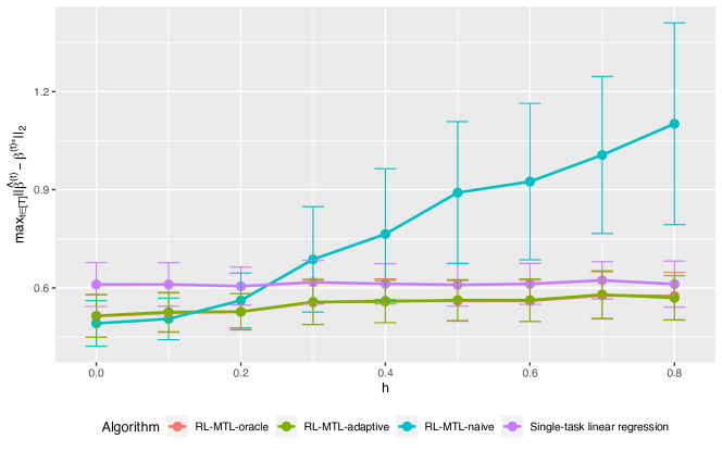
Figure 3: Simulation with no outlier tasks: estimation error $\max_{t\in[T]}\|\widehat{\bm{\beta}}^{(t)}-\bm{\beta}^{(t)*}\|_{2}$ of four algorithms. The point and error bar represent the average error and standard deviation over 200 replications, respectively. Note that curves of RL-MTL-oracle and RL-MTL-adaptive overlap with each other substantially.

6.2 With Outlier Tasks

In the second example, we have a total of $T=7$ tasks, with the first six tasks the same as in the first example and the last task as an outlier. The outlier task is generated from the linear model (2) as the other tasks, but without the low-dimensional structure. Specifically, each entry of $\bm{\beta}^{(7)*}$ is i.i.d. generated from Unif$(-1,1)$ in each replication, and $\epsilon^{(7)}_{i}$ is i.i.d. from $N(0,1)$.

Unlike the case with no outlier tasks, Figures 4 and 5 show that with one outlier task, even when $h=0$, RL-MTL-naive can perform much worse than single-task linear regression. However, our proposed algorithms, RL-MTL-oracle and RL-MTL-adaptive, still outperform single-task linear regression, validating the robustness against outlier tasks as our theory indicates. Moreover, we observe that the performances of RL-MTL-oracle and RL-MTL-adaptive are comparable, which suggests that our adaptation algorithm (Algorithm 3) is effective in estimating the unknown $r$ with outlier tasks.

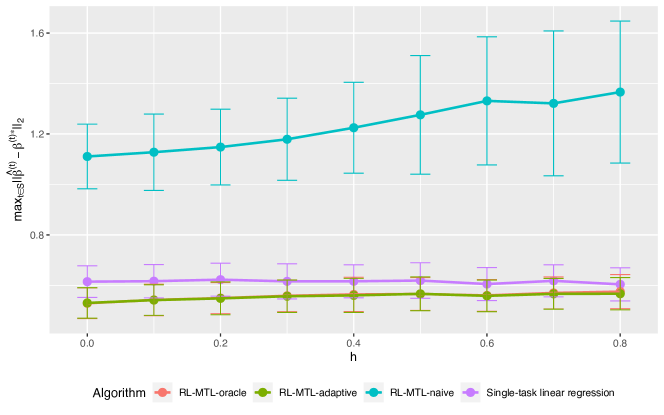
Figure 4: Simulation with one outlier task: estimation error $\max_{t\in S}\|\widehat{\bm{\beta}}^{(t)}-\bm{\beta}^{(t)*}\|_{2}$ of four algorithms. The point and error bar represent the average error and standard deviation over 200 replications, respectively. Note that curves of RL-MTL-oracle and RL-MTL-adaptive overlap with each other substantially.

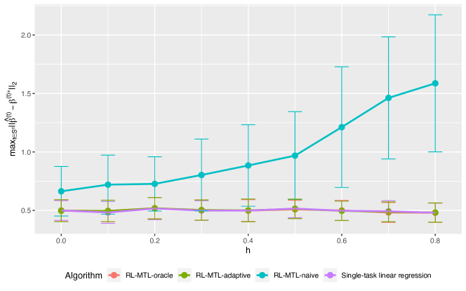
Figure 5: Simulation with one outlier task: estimation error $\max_{t\in S^{c}}\|\widehat{\bm{\beta}}^{(t)}-\bm{\beta}^{(t)*}\|_{2}$ of four algorithms. The point and error bar represent the average error and standard deviation over 200 replications, respectively. Note that curves of RL-MTL-oracle and RL-MTL-adaptive overlap with each other substantially.

7 Discussions

In this work, we investigated the representation multi-task and transfer learning problem, where most tasks share similar linear representations and a small fraction of tasks can be arbitrarily contaminated. To address this problem, we proposed two-step algorithms under MTL and TL settings, and derived upper bounds for the estimation error. Our results demonstrated that the algorithms are adaptive to the problem structure and robust to a small fraction of outlier tasks. Moreover, we presented the first lower bound results for estimating regression coefficients in the context of representation MTL and TL. In a large regime, our algorithms are nearly minimax optimal. We extended the algorithms and theory to GLMs and non-linear regression models. Finally, we proposed a simple yet effective algorithm to adapt our MTL and TL algorithms to the case of an unknown intrinsic dimension $r$.

Acknowledgments

Ye Tian is grateful to Gan Yuan (Columbia) and Yasaman Mahdaviyeh (Columbia) for a lot of valuable discussions which greatly improved the quality of this paper. Ye Tian also wants to thank Prof. Linjun Zhang (Rutgers) whose insightful discussions initially inspired this work. All the simulations were conducted on Ginsburg HPC cluster of Columbia University. Yuqi Gu acknowledges the support of the NSF Grant DMS-2210796. Yang Feng’s research is partially supported by by NIH grant 1R21AG074205-01, NYU University Research Challenge Fund, and a grant from NYU School of Global Public Health.

A General Lemmas

A.1 Lemmas

Lemma 27 (Theorem 6.5 in [57])

Suppose that Assumptions 1 and 3 hold. Then for any $\delta>0$ and any $t\in[T]$, w.p. at least $1-C_{1}e^{-nC_{2}(\delta\wedge\delta^{2})}$,

$$\|\widehat{\bm{\Sigma}}^{(t)}-\bm{\Sigma}^{(t)}\|_{2}\leq C_{3}\sqrt{\frac{p}{n}}+\delta,$$ (22)

with some constants $C_{1},C_{2},C_{3}>0$. Note that $C_{1},C_{2},C_{3}$ are universal in the sense that they do not depend on $t$ or $\delta$. As a consequence, we have

$$\max_{t\in[T]}\|\widehat{\bm{\Sigma}}^{(t)}-\bm{\Sigma}^{(t)}\|_{2}\lesssim\sqrt{\frac{p+\log T}{n}},$$ (23)

w.p. at least $1-e^{-C(p+\log T)}$.

Lemma 28 (A variant of Theorem 6.5 in [57])

Suppose that Assumptions 4 and 6 hold. Then for any $\delta>0$, for any fixed $\bm{A},\bm{B}\in\mathcal{O}^{p\times r}$, w.p. at least $1-C_{1}e^{-n_{0}C_{2}(\delta\wedge\delta)}$,

$$\|\bm{A}^{T}\widehat{\bm{\Sigma}}^{(t)}\bm{B}-\bm{A}^{T}\bm{\Sigma}^{(t)}\bm{B}\|_{2}\leq C_{3}\sqrt{\frac{r}{n_{0}}}+\delta,$$ (24)

with some constants $C_{1},C_{2},C_{3}>0$. Note that $C_{1},C_{2},C_{3}$ are universal in the sense that they do not depend on $\delta$ or $t$. As a consequence, for any fixed $\bm{A},\bm{B}\in\mathcal{O}^{p\times r}$, we have

$$\|\bm{A}^{T}\widehat{\bm{\Sigma}}^{(0)}\bm{B}-\bm{A}^{T}\bm{\Sigma}^{(0)}\bm{B}\|_{2}\lesssim\sqrt{\frac{r}{n_{0}}},$$ (25)

w.p. at least $1-e^{-C(r+\log T)}$.

Lemma 29 (Lemmas 2.5 and 2.6 in [12])

Suppose $p\geq r$. Consider two matrics $\bm{A},\widetilde{\bm{A}}\in\mathcal{O}^{p\times r}$. Suppose that $(\bm{A},\bm{A}^{\perp}),(\widetilde{\bm{A}},\widetilde{\bm{A}}^{\perp})\in\mathbb{R}^{p\times p}$ are both orthonormal matrices, which means that $\bm{A}^{\perp}$ and $\widetilde{\bm{A}}^{\perp}$ are orthonormal complements of $\bm{A}$ and $\widetilde{\bm{A}}$, respectively. Then

$$\|\bm{A}\bm{A}^{T}-\widetilde{\bm{A}}(\widetilde{\bm{A}})^{T}\|_{2} =\|\bm{A}^{T}(\widetilde{\bm{A}}^{\perp})\|_{2}=\|(\widetilde{\bm{A}})^{T}\bm{A}^{\perp}\|_{2},$$ (26)

$$\frac{1}{\sqrt{2}}\|\bm{A}\bm{A}^{T}-\widetilde{\bm{A}}(\widetilde{\bm{A}})^{T}\|_{\textup{F}} =\|\bm{A}^{T}(\widetilde{\bm{A}}^{\perp})\|_{\textup{F}}=\|(\widetilde{\bm{A}})^{T}\bm{A}^{\perp}\|_{\textup{F}},$$ (27)

$$\|\bm{A}\bm{A}^{T}-\widetilde{\bm{A}}(\widetilde{\bm{A}})^{T}\|_{2} \leq\min_{\bm{R}\in\mathcal{O}^{r\times r}}\|\bm{A}-\widetilde{\bm{A}}\bm{R}\|_{2}\leq\sqrt{2}\|\bm{A}\bm{A}^{T}-\widetilde{\bm{A}}(\widetilde{\bm{A}})^{T}\|_{2},$$ (28)

$$\frac{1}{\sqrt{2}}\|\bm{A}\bm{A}^{T}-\widetilde{\bm{A}}(\widetilde{\bm{A}})^{T}\|_{\textup{F}} \leq\min_{\bm{R}\in\mathcal{O}^{r\times r}}\|\bm{A}-\widetilde{\bm{A}}\bm{R}\|_{\textup{F}}\leq\|\bm{A}\bm{A}^{T}-\widetilde{\bm{A}}(\widetilde{\bm{A}})^{T}\|_{\textup{F}}.$$ (29)

Lemma 30 (Proposition 8 in [44])

When $p\geq 2r$, for any $\delta>0$, we have

1. $C_{1}(\frac{\sqrt{r}}{8})^{r(p-r)}\leq N(\mathcal{O}^{p\times r},\textup{dist}_{\textup{F}},\delta)\leq C_{2}(\frac{\sqrt{r}}{8})^{r(p-r)}$;

2. $C_{1}(\frac{1}{8})^{r(p-r)}\leq N(\mathcal{O}^{p\times r},\textup{dist}_{2},\delta)\leq C_{2}(\frac{1}{8})^{r(p-r)}$;

3. (Consequence of (i)) $M(\mathcal{O}^{p\times r},\textup{dist}_{\textup{F}},\delta)\geq C(\frac{\sqrt{r}}{8})^{r(p-r)}$.

Lemma 31

When $p\geq 2r$, for any $\delta>0$ and $\alpha\in(0,1)$, $\exists\macc@depth\char 1\relax\frozen@everymath{\macc@group}\macc@set@skewchar\macc@nested@a 111{}\in\mathcal{O}^{p\times r}$, such that

$$M(\mathcal{B}_{\delta}(\macc@depth\char 1\relax\frozen@everymath{\macc@group}\macc@set@skewchar\macc@nested@a 111{},\mathcal{O}^{p\times r},\textup{dist}_{2}),\textup{dist}_{\textup{F}},\alpha\delta)\geq\left(\frac{C\sqrt{r}}{\alpha}\right)^{r(p-r)}.$$ (30)

Lemma 32 (Fano’s lemma, see [54] and [57])

Suppose $(\Theta,d)$ is a metric space and each $\theta$ in this space is associated with a probability measure $\mathbb{P}_{\theta}$. If $\{\theta_{j}\}_{j=1}^{N}$ is an $s$-separated set (i.e. $d(\theta_{j},\theta_{k})\geq s$ for any $j\neq k$), and $\textup{KL}(\mathbb{P}_{\theta_{j}},\mathbb{P}_{\theta_{k}})\leq\alpha\log N$, then

$$\inf_{\widehat{\theta}}\sup_{\theta\in\Theta}\mathbb{P}_{\theta}(d(\widehat{\theta},\theta)\geq s/2)\geq 1-\alpha-\frac{\log 2}{\log N}.$$ (31)

Lemma 33

Consider the following generative model:

$$y|\bm{x}\sim\mathbb{P}_{y|\bm{x},\bm{\beta}}=N(\bm{x}^{T}\bm{\beta},1),\quad\bm{x}\sim\mathbb{P}_{\bm{x}},$$ (32)

where $\mathbb{P}_{\bm{x}}$ is sub-Gaussian with $\bm{\Sigma}=\mathbb{E}(\bm{x}\bm{x}^{T})$. Suppose there exist constants $c$ and $C$ such that $0<c\leq\lambda_{\min}(\bm{\Sigma})\leq\lambda_{\max}(\bm{\Sigma})\leq C<\infty$. Define two distributions $\mathbb{P}$ and $\widetilde{\mathbb{P}}$ of $(\bm{x},y)$ as $\mathbb{P}_{\bm{x},y}=\mathbb{P}_{y|\bm{x};\bm{\beta}}\cdot\mathbb{P}_{\bm{x}}$ and $\widetilde{\mathbb{P}}_{\bm{x},y}=\mathbb{P}_{y|\bm{x};\widetilde{\bm{\beta}}}\cdot\mathbb{P}_{\bm{x}}$. Then, the KL divergence between $\mathbb{P}_{\bm{x},y}$ and $\widetilde{\mathbb{P}}_{\bm{x},y}$ can be bounded as

$$\textup{KL}(\mathbb{P}_{\bm{x},y}\|\widetilde{\mathbb{P}}_{\bm{x},y})\leq C\|\bm{\beta}-\widetilde{\bm{\beta}}\|_{2}^{2}.$$ (33)

Lemma 34 (Theorem 5.1 in [9])

Given a family of distributions $\{\mathbb{P}_{\theta}:\theta\in\Theta\}$, which is indexed by a parameter $\theta\in\Theta$. Consider $\bm{x}^{(t)}\sim(1-\epsilon^{\prime})\mathbb{P}_{\theta}+\epsilon^{\prime}\mathbb{Q}$ independently for $t\in[T]$, and $\widetilde{\bm{x}}\sim\mathbb{P}_{\widetilde{\bm{x}}}$. Denote the joint distribution of $\{\bm{x}^{(t)}\}_{t=1}^{T}$ and $\widetilde{x}$ as $\mathbb{P}_{(\epsilon^{\prime},\theta,\mathbb{Q})}\cdot\mathbb{P}_{\widetilde{\bm{x}}}$. Then

$$\inf_{\widehat{\theta}}\sup_{\begin{subarray}{c}\theta\in\Theta\\ \mathbb{Q}\end{subarray}}(\mathbb{P}_{(\epsilon^{\prime},\theta,\mathbb{Q})}\cdot\mathbb{P}_{\widetilde{\bm{x}}})\left(\|\widehat{\theta}-\theta\|\geq C\varpi(\epsilon^{\prime},\Theta)\right)\geq\frac{1}{2},$$ (34)

where $\varpi(\epsilon^{\prime},\Theta)\coloneqq\sup\{\|\theta_{1}-\theta_{2}\|:\textup{TV}\big{(}\mathbb{P}_{\theta_{1}},\mathbb{P}_{\theta_{2}}\big{)}\leq\epsilon^{\prime}/(1-\epsilon^{\prime}),\theta_{1},\theta_{2}\in\Theta\}$.

Lemma 35 (Lemma 22 in [51])

Consider two data generating mechanisms:

1. $\bm{x}^{(t)}\sim(1-\epsilon^{\prime})\mathbb{P}_{\theta}+\epsilon^{\prime}\mathbb{Q}$ independently for $t\in[T]$, where $\epsilon^{\prime}=\frac{|S^{c}|}{T}$, and $\widetilde{x}\sim\mathbb{P}_{\widetilde{\bm{x}}}$;

2. With a preserved set $S\subseteq[T]$, generate $\{\bm{x}^{(t)}\}_{t\in S^{c}}\sim\mathbb{Q}_{S^{c}}$ and $\bm{x}^{(t)}\sim\mathbb{P}_{\theta}$ independently for $t\in S$, and $\widetilde{x}\sim\mathbb{P}_{\widetilde{\bm{x}}}$.

Denote the joint distributions of $\{\bm{x}^{(t)}\}_{t=1}^{T}$ and $\widetilde{x}$ in (i) and (ii) as $\mathbb{P}_{(\epsilon,\theta,\mathbb{Q})}\cdot\mathbb{P}_{\widetilde{\bm{x}}}$ and $\mathbb{P}_{(S,\theta,\mathbb{Q}_{S^{c}})}\cdot\mathbb{P}_{\widetilde{\bm{x}}}$, respectively. We claim that if

$$\inf_{\widehat{\theta}}\sup_{\begin{subarray}{c}\theta\in\Theta\\ \mathbb{Q}\end{subarray}}(\mathbb{P}_{(\epsilon^{\prime}/50,\theta,\mathbb{Q})}\cdot\mathbb{P}_{\widetilde{\bm{x}}})\left(\|\widehat{\theta}-\theta\|\geq C\varpi(\epsilon^{\prime}/50,\Theta)\right)\geq\frac{1}{2}$$ (35)

then

$$\inf_{\widehat{\theta}}\sup_{S:|S|\geq T(1-\epsilon^{\prime})}\sup_{\begin{subarray}{c}\theta\in\Theta\\ \mathbb{Q}_{S^{c}}\end{subarray}}(\mathbb{P}_{(S,\theta,\mathbb{Q}_{S^{c}})}\cdot\mathbb{P}_{\widetilde{\bm{x}}})\left(\|\widehat{\theta}-\theta\|\geq C\varpi\left(\epsilon^{\prime}/50,\Theta\right)\right)\geq\frac{1}{10},$$ (36)

where $\varpi(\epsilon^{\prime},\Theta)\coloneqq\sup\{\|\theta_{1}-\theta_{2}\|:\textup{TV}\big{(}\mathbb{P}_{\theta_{1}},\mathbb{P}_{\theta_{2}}\big{)}\leq\epsilon^{\prime}/(1-\epsilon^{\prime}),\theta_{1},\theta_{2}\in\Theta\}$.

Lemma 36 (Lemma 33 in [51])

Given a family of distributions $\{\mathbb{P}_{\theta}:\theta\in\Theta\}$, which is indexed by a parameter $\theta\in\Theta$. Consider $\bm{x}^{(t)}\sim(1-\epsilon^{\prime})\mathbb{P}_{\theta}+\epsilon^{\prime}\mathbb{Q}$ independently for $t\in[T]$, and $\widetilde{x}\sim\mathbb{P}_{\widetilde{\bm{x}}}$. Consider another family of distributions $\{\mathbb{P}_{\theta}^{(0)}:\theta\in\Theta\}$ indexed by the same parameter set, and $\bm{x}^{(0)}\sim\mathbb{P}_{\theta}^{(0)}$. Denote the joint distribution of $\{\bm{x}^{(t)}\}_{t=0}^{T}$ and $\widetilde{x}$ as $\mathbb{P}_{(\epsilon^{\prime},\theta,\mathbb{Q})}\cdot\mathbb{P}_{\widetilde{\bm{x}}}$. Then

$$\inf_{\widehat{\theta}}\sup_{\begin{subarray}{c}\theta\in\Theta\\ \mathbb{Q}\end{subarray}}(\mathbb{P}_{(\epsilon^{\prime},\theta,\mathbb{Q})}\cdot\mathbb{P}_{\widetilde{\bm{x}}})\left(\|\widehat{\theta}-\theta\|\geq C\varpi(\epsilon^{\prime},\Theta)\right)\geq\frac{9}{20},$$ (37)

where $\varpi(\epsilon^{\prime},\Theta)\coloneqq\sup\big{\{}\|\theta_{1}-\theta_{2}\|:\textup{TV}\big{(}\mathbb{P}_{\theta_{1}},\mathbb{P}_{\theta_{2}}\big{)}\leq\epsilon^{\prime}/(1-\epsilon^{\prime}),\textup{TV}\big{(}\mathbb{P}^{(0)}_{\theta_{1}},\mathbb{P}^{(0)}_{\theta_{2}}\big{)}\leq 1/20,\theta_{1},\theta_{2}\in\Theta\big{\}}$.

Lemma 37 (Lemma 34 in [51])

Consider two data generating mechanisms:

1. $\bm{x}^{(t)}\sim(1-\epsilon^{\prime})\mathbb{P}_{\theta}+\epsilon^{\prime}\mathbb{Q}$ independently for $t\in[T]$, $\bm{x}^{(0)}\sim\mathbb{P}^{(0)}_{\theta}$, and $\widetilde{x}\sim\mathbb{P}_{\widetilde{\bm{x}}}$, where $\epsilon^{\prime}=\frac{|S^{c}|}{T}$;

2. With a preserved set $S\subseteq[T]$, generate $\{\bm{x}^{(t)}\}_{t\in S^{c}}\sim\mathbb{Q}_{S^{c}}$ and $\bm{x}^{(t)}\sim\mathbb{P}_{\theta}$ independently for $t\in S$, $\bm{x}^{(0)}\sim\mathbb{P}^{(0)}_{\theta}$, and $\widetilde{x}\sim\mathbb{P}_{\widetilde{\bm{x}}}$.

Denote the joint distributions of $\{\bm{x}^{(t)}\}_{t=0}^{T}$ and $\widetilde{x}$ in (i) and (ii) as $\mathbb{P}_{(\epsilon,\theta,\mathbb{Q})}\cdot\mathbb{P}_{\widetilde{\bm{x}}}$ and $\mathbb{P}_{(S,\theta,\mathbb{Q}_{S^{c}})}\cdot\mathbb{P}_{\widetilde{\bm{x}}}$, respectively. We claim that if

$$\inf_{\widehat{\theta}}\sup_{\begin{subarray}{c}\theta\in\Theta\\ \mathbb{Q}\end{subarray}}(\mathbb{P}_{(\epsilon^{\prime}/50,\theta,\mathbb{Q})}\cdot\mathbb{P}_{\widetilde{\bm{x}}})\left(\|\widehat{\theta}-\theta\|\geq C\varpi^{\prime}\left(\epsilon^{\prime}/50,\Theta\right)\right)\geq\frac{9}{20},$$ (38)

then

$$\inf_{\widehat{\theta}}\sup_{S:|S|\geq T(1-\epsilon^{\prime})}\sup_{\begin{subarray}{c}\theta\in\Theta\\ \mathbb{Q}_{S}\end{subarray}}(\mathbb{P}_{(S,\theta,\mathbb{Q}_{S})}\cdot\mathbb{P}_{\widetilde{\bm{x}}})\left(\|\widehat{\theta}-\theta\|\geq C\varpi^{\prime}\left(\epsilon^{\prime}/50,\Theta\right)\right)\geq\frac{1}{10},$$ (39)

where $\varpi(\epsilon^{\prime},\Theta)\coloneqq\sup\big{\{}\|\theta_{1}-\theta_{2}\|:\textup{TV}\big{(}\mathbb{P}_{\theta_{1}}\|\mathbb{P}_{\theta_{2}}\big{)}\leq\epsilon^{\prime}/(1-\epsilon^{\prime}),\textup{TV}\big{(}\mathbb{P}^{(0)}_{\theta_{1}}\|\mathbb{P}^{(0)}_{\theta_{2}}\big{)}\leq 1/20,\theta_{1},\theta_{2}\in\Theta\big{\}}$.

A.2 Proofs of Lemmas

Denote $\widehat{\bm{\Sigma}}^{(t)}=\sum_{i=1}^{n}\frac{1}{n}\bm{x}^{(t)}_{i}(\bm{x}^{(t)}_{i})^{T}$.

A.2.1 Proof of Lemma 28

Note that for any fixed $\bm{A},\bm{B}\in\mathcal{O}^{p\times r}$,

$$\|\bm{A}^{T}(\widehat{\bm{\Sigma}}^{(0)}-\bm{\Sigma}^{(0)})\bm{B}\|_{2}=\sup_{\|\bm{u}\|_{2},\|\bm{v}\|_{2}\leq 1}(\bm{A}\bm{u})^{T}(\widehat{\bm{\Sigma}}^{(0)}-\bm{\Sigma}^{(0)})(\bm{B}\bm{v}),$$ (40)

where $\bm{A}\bm{u},\bm{B}\bm{v}\in\mathbb{R}^{p}$ and $\|\bm{A}\bm{u}\|_{2}=\|\bm{B}\bm{v}\|_{2}=1$. Note that both $\bm{A}\bm{u}$ and $\bm{B}\bm{v}$ live in $r$-dimensional space (isomorphic to the unit ball in $\mathbb{R}^{r}$). Therefore, by Example 5.8 in [57], there exist two $1/8$-covers (whose components are inside the set to be covered) of $\{\bm{\beta}\in\mathbb{R}:\bm{\beta}=\bm{A}\bm{u},\|\bm{u}\|_{2}\leq 1\}$ and $\{\bm{\beta}\in\mathbb{R}:\bm{\beta}=\bm{B}\bm{u},\|\bm{u}\|_{2}\leq 1\}$ under Euclidean norm, denoted as $\{\bm{\beta}_{j}^{\bm{u}}\}_{j=1}^{N_{1}}$ and $\{\bm{\beta}_{j}^{\bm{u}}\}_{j=1}^{N_{2}}$, respectively, such that $|N_{1}|=|N_{2}|\leq 17^{r}$. Then we can proceed in the same steps as in the proof of Theorem 6.5 in [57] to finish the proof.

A.2.2 Proof of Lemma 31

We apply the same trick as in the proof of Proposition 3 in [8]. Suppose the minimum cover of $\mathcal{O}^{p\times r}$ under $\textup{dist}_{2}(\cdot)$ corresponding to $N(\mathcal{O}^{p\times r},\textup{dist}_{2},\delta)$ is $\mathcal{N}$. By pigeonhole theorem, for any $\alpha\in(0,1)$,

$$N(\mathcal{O}^{p\times r},\textup{dist}_{2},\alpha\delta) \leq N(\cup_{\bm{A}\in\mathcal{N}}\mathcal{B}_{\delta}(\bm{A},\mathcal{O}^{p\times r},\textup{dist}_{2}),\textup{dist}_{\textup{F}},\alpha\delta)$$ (41)

$$\leq|\mathcal{N}|\max_{\bm{A}\in\mathcal{N}}N(\mathcal{B}_{\delta}(\bm{A},\mathcal{O}^{p\times r},\textup{dist}_{2}),\textup{dist}_{\textup{F}},\alpha\delta).$$ (42)

Then applying Lemma 30 leads to

$$\max_{\bm{A}\in\mathcal{N}}N(\mathcal{B}_{\delta}(\bm{A},\mathcal{O}^{p\times r},\textup{dist}_{2}),\textup{dist}_{\textup{F}},\alpha\delta)\geq\frac{N(\mathcal{O}^{p\times r},\textup{dist}_{2},\alpha\delta)}{N(\mathcal{O}^{p\times r},\textup{dist}_{2},\delta)}\geq\left(\frac{C\sqrt{r}}{\alpha}\right)^{r(p-r)}.$$ (43)

Since $\mathcal{N}$ has only finite elements, there must exist one $\bm{A}\in\mathcal{N}$ achieving the maximum of LHS. Because the packing number is always larger than or equal to the covering number, the proof is done.

A.2.3 Proof of Lemma 33

By the form of Gaussian density function, it is straightfoward to see that

$$\textup{KL}(\mathbb{P}_{\bm{x},y}\|\widetilde{\mathbb{P}}_{\bm{x},y}) =\int\log\left(\frac{\mathbb{P}_{y|\bm{x},\bm{\beta}}}{\mathbb{P}_{y|\bm{x},\widetilde{\bm{\beta}}}}\right)\textup{d}\mathbb{P}_{y|\bm{x},\bm{\beta}}\textup{d}\mathbb{P}_{\bm{x}}$$ (44)

$$\leq\underbrace{\int(y-\bm{x}^{T}\bm{\beta})\cdot\bm{x}^{T}(\bm{\beta}-\widetilde{\bm{\beta}})\textup{d}\mathbb{P}_{y|\bm{x},\bm{\beta}}\textup{d}\mathbb{P}_{\bm{x}}}_{=0}+\int[\bm{x}^{T}(\bm{\beta}-\widetilde{\bm{\beta}})]^{2}\textup{d}\mathbb{P}_{\bm{x}}$$ (45)

$$\lesssim\|\bm{\beta}-\widetilde{\bm{\beta}}\|_{2}^{2}.$$ (46)

B Proofs for Linear Regression Models

Denote $\bm{\theta}^{(t)}_{\bm{A}}\in\operatorname*{arg\,min}_{\bm{\theta}\in\mathbb{R}^{r}}f^{(t)}(\bm{A}\bm{\theta})$ and $f^{(t)}(\bm{\beta})=\frac{1}{n}\|\bm{Y}^{(t)}-\bm{X}^{(t)}\bm{\beta}\|_{2}^{2}$. For $\bm{A},\widetilde{\bm{A}}\in\mathcal{O}^{p\times r}$, define metrics $\textup{dist}_{2}(\bm{A},\widetilde{\bm{A}})=\|\bm{A}\bm{A}^{T}-\widetilde{\bm{A}}(\widetilde{\bm{A}})^{T}\|_{2}$, $\textup{dist}_{\textup{F}}(\bm{A},\widetilde{\bm{A}})=\|\bm{A}\bm{A}^{T}-\widetilde{\bm{A}}(\widetilde{\bm{A}})^{T}\|_{\textup{F}}$. In any metric space $(\mathcal{X},\rho)$, denote the ball of radius $\delta$ with center $x$ under metric $\rho$ as $\mathcal{B}_{\delta}(x,\mathcal{X},\rho)$.

B.1 Lemmas

Lemma 38

Suppose Assumptions 1-3 hold. Then w.p. at least $1-e^{-C(r+\log T)}$, for all $t\in[T]$ and $\bm{A}\in\mathcal{O}^{p\times r}$,

$$\|\bm{A}\bm{\theta}^{(t)}_{\bm{A}}-\bm{A}^{(t)*}\bm{\theta}^{(t)*}\|_{2}\lesssim\|\bm{A}\bm{A}^{T}-\bm{A}^{(t)*}(\bm{A}^{(t)*})^{T}\|_{2}+\sqrt{\frac{r+\log T}{n}}.$$ (47)

Lemma 39

Suppose Assumptions 1-3 hold. Then w.p. at least $1-e^{-C(r+\log T)}$, for all $t\in S$ and $\bm{A}\in\mathcal{O}^{p\times r}$, there exists a universal constant $C^{\prime}>0$ (which does not depend on $t$ or $\bm{A}$), such that $\|\bm{A}\bm{\theta}^{(t)}_{\bm{A}}\|_{2}=\|\bm{\theta}^{(t)}_{\bm{A}}\|_{2}\leq C^{\prime}$.

Lemma 40

Suppose Assumptions 1-3 hold. Then w.p. at least $1-e^{-C(r+\log T)}$, for all $t\in[T]$ and $\bm{A},\widetilde{\bm{A}}\in\mathcal{O}^{p\times r}$,

$$\|\bm{A}\bm{\theta}^{(t)}_{\bm{A}}-\widetilde{\bm{A}}\bm{\theta}^{(t)}_{\widetilde{\bm{A}}}\|_{2}\lesssim\|\bm{A}\bm{A}^{T}-\widetilde{\bm{A}}\widetilde{\bm{A}}^{T}\|_{2}(1+\|\nabla f^{(t)}(\widetilde{\bm{A}}\bm{\theta}^{(t)}_{\widetilde{\bm{A}}})\|_{2}).$$ (48)

Lemma 41

Suppose Assumptions 1-3 hold. For any $\macc@depth\char 1\relax\frozen@everymath{\macc@group}\macc@set@skewchar\macc@nested@a 111{}\in\operatorname*{arg\,min}_{\macc@depth\char 1\relax\frozen@everymath{\macc@group}\macc@set@skewchar\macc@nested@a 111{}\in\mathcal{O}^{p\times r}}\max_{t\in S}\{\|\bm{A}^{(t)}(\bm{A}^{(t)})^{T}-\macc@depth\char 1\relax\frozen@everymath{\macc@group}\macc@set@skewchar\macc@nested@a 111{}{\macc@depth\char 1\relax\frozen@everymath{\macc@group}\macc@set@skewchar\macc@nested@a 111{}}^{T}\|_{2}\}$, denote $\macc@depth\char 1\relax\frozen@everymath{\macc@group}\macc@set@skewchar\macc@nested@a 111{}=\big{\{}\nabla f^{(t)}(\macc@depth\char 1\relax\frozen@everymath{\macc@group}\macc@set@skewchar\macc@nested@a 111{}\bm{\theta}^{(t)}_{\macc@depth\char 1\relax\frozen@everymath{\macc@group}\macc@set@skewchar\macc@nested@a 111{}})\big{\}}_{t\in S}$, then w.p. at least $1-e^{-C(p+\log T)}$,

$$\|\macc@depth\char 1\relax\frozen@everymath{\macc@group}\macc@set@skewchar\macc@nested@a 111{}\|_{2}\lesssim\sqrt{\frac{p}{n}}+\sqrt{T}\left(h+\sqrt{\frac{r+\log T}{n}}\right).$$ (49)

Lemma 42

Suppose $\bm{G}=\{\bm{g}_{j}\}_{j=1}^{d}\in\mathbb{R}^{p\times d}$ and $\macc@depth\char 1\relax\frozen@everymath{\macc@group}\macc@set@skewchar\macc@nested@a 111{}=\{\macc@depth\char 1\relax\frozen@everymath{\macc@group}\macc@set@skewchar\macc@nested@a 111{}_{j}\}_{j=1}^{d}\in\mathbb{R}^{p\times d}$ with each $\bm{g}_{j},\macc@depth\char 1\relax\frozen@everymath{\macc@group}\macc@set@skewchar\macc@nested@a 111{}_{j}\in\mathbb{R}^{p}$ and $\max_{j\in[d]}\|\bm{g}_{j}-\macc@depth\char 1\relax\frozen@everymath{\macc@group}\macc@set@skewchar\macc@nested@a 111{}_{j}\|_{2}\leq\Delta$. Then

$$\|\macc@depth\char 1\relax\frozen@everymath{\macc@group}\macc@set@skewchar\macc@nested@a 111{}-\bm{G}\|_{2}\leq\sqrt{d}\Delta.$$ (50)

Lemma 43

Suppose Assumptions 1-3 hold. Consider any $\widehat{\macc@depth\char 1\relax\frozen@everymath{\macc@group}\macc@set@skewchar\macc@nested@a 111{}}\in\mathcal{O}^{p\times r}$. When $\frac{\lambda}{\sqrt{n}}\geq C\|\widehat{\macc@depth\char 1\relax\frozen@everymath{\macc@group}\macc@set@skewchar\macc@nested@a 111{}}\bm{\theta}^{(t)}_{\widehat{\macc@depth\char 1\relax\frozen@everymath{\macc@group}\macc@set@skewchar\macc@nested@a 111{}}}-\bm{A}^{(t)*}\bm{\theta}^{(t)*}\|_{2}+\|\nabla f^{(t)}(\bm{A}^{(t)*}\bm{\theta}^{(t)*})\|_{2}$ with a sufficiently large $C$, for any $t\in S$ and the minimizer $(\bm{A}^{(t)},\bm{\theta}^{(t)})=\operatorname*{arg\,min}_{\bm{A}\in\mathcal{O}^{p\times r},\bm{\theta}\in\mathbb{R}^{r}}\{\frac{1}{T}f^{(t)}(\bm{A}\bm{\theta})+\frac{\sqrt{n}}{nT}\lambda\|\bm{A}\bm{A}^{T}-\widehat{\macc@depth\char 1\relax\frozen@everymath{\macc@group}\macc@set@skewchar\macc@nested@a 111{}}(\widehat{\macc@depth\char 1\relax\frozen@everymath{\macc@group}\macc@set@skewchar\macc@nested@a 111{}})^{T}\|_{2}\}$, we must have $\bm{A}^{(t)}(\bm{A}^{(t)})^{T}=\widehat{\macc@depth\char 1\relax\frozen@everymath{\macc@group}\macc@set@skewchar\macc@nested@a 111{}}(\widehat{\macc@depth\char 1\relax\frozen@everymath{\macc@group}\macc@set@skewchar\macc@nested@a 111{}})^{T}$. As a consequence, by Lemma 38, when $\lambda\geq C\sqrt{p+\log T}$ and $\|\widehat{\macc@depth\char 1\relax\frozen@everymath{\macc@group}\macc@set@skewchar\macc@nested@a 111{}}(\widehat{\macc@depth\char 1\relax\frozen@everymath{\macc@group}\macc@set@skewchar\macc@nested@a 111{}})^{T}-\bm{A}^{(t)*}(\bm{A}^{(t)*})^{T}\|_{2}\lesssim\sqrt{\frac{p+\log T}{n}}$, w.p. at least $1-e^{-C(r+\log T)}$, we have $\bm{A}^{(t)}(\bm{A}^{(t)})^{T}=\widehat{\macc@depth\char 1\relax\frozen@everymath{\macc@group}\macc@set@skewchar\macc@nested@a 111{}}(\widehat{\macc@depth\char 1\relax\frozen@everymath{\macc@group}\macc@set@skewchar\macc@nested@a 111{}})^{T}$ for all $t\in S$.

Lemma 44

Under Assumption 2, for any subset $S^{\prime}\subset S$ with $|S^{\prime}|\geq(1-\alpha)|S|$ and $\alpha\leq c/r$ ($c$ is a sufficiently small positive constant), we have

$$\frac{1}{|S^{\prime}|}\sum_{t\in S^{\prime}}\bm{\theta}^{(t)*}(\bm{\theta}^{(t)*})^{T}\succeq\frac{c^{\prime}}{r}\bm{I}_{r},$$ (51)

with some constant $c^{\prime}>0$.

Lemma 45

Under Assumptions 1-3, w.p. at least $1-e^{-C(p+\log T)}$, for all $t\in S$,

$$\|\widehat{\bm{A}}^{(t)}\widehat{\bm{\theta}}^{(t)}-\bm{A}^{(t)*}\bm{\theta}^{(t)*}\|_{2}\lesssim\left(\frac{\lambda}{\sqrt{n}}\right)^{1/2}+\sqrt{\frac{p+\log T}{n}}.$$ (52)

Lemma 46

Consider the case that $r=1$. Suppose that $\min_{t\in S}|\bm{\theta}^{(t)*}|\geq c>0$ with some constant $c>0$. Under Assumptions 1-3, w.p. at least $1-e^{-C^{\prime}(1+\log T)}$, for all $\bm{A}\in\mathcal{O}^{p\times r}$ and $t\in S$,

$$\|\bm{A}\bm{\theta}^{(t)}_{\bm{A}}-\bm{A}^{(t)*}\bm{\theta}^{(t)*}\|_{2}\geq c\|\bm{A}\bm{A}^{T}-\bm{A}^{(t)*}(\bm{A}^{(t)*})^{T}\|_{2}-C\sqrt{\frac{p+\log T}{n}}.$$ (53)

Lemma 47 (For MTL)

Under Assumptions 1-3, we have:

1. For all $t\in S$, when $\frac{\gamma}{\sqrt{n}}\geq\|\nabla f^{(t)}(\bm{A}^{(t)*}\bm{\theta}^{(t)*})\|_{2}+C\|\widehat{\bm{A}}^{(t)}\widehat{\bm{\theta}}^{(t)}-\bm{A}^{(t)*}\bm{\theta}^{(t)*}\|_{2}$, it holds that $\widehat{\bm{\beta}}^{(t)}=\widehat{\bm{A}}^{(t)}\widehat{\bm{\theta}}^{(t)}$ w.p. at least $1-e^{-C(p+\log T)}$;

2. $\max_{t\in S}\|\widehat{\bm{\beta}}^{(t)}-\bm{\beta}^{(t)*}\|_{2}\leq C\frac{\gamma}{\sqrt{n}}+\max_{t\in S}\|\widetilde{\bm{\beta}}^{(t)}-\bm{\beta}^{(t)*}\|_{2}$ w.p. at least $1-e^{-C(p+\log T)}$, where $\widetilde{\bm{\beta}}^{(t)}\in\operatorname*{arg\,min}_{\bm{\beta}\in\mathbb{R}^{p}}f^{(t)}(\bm{\beta})$;

3. If the data from tasks in $S^{c}$ satisfies the linear model (2) (without any latent structure assumption) and Assumption 1, then w.p. at least $1-e^{-C(p+\log T)}$, $\max_{t\in S^{c}}\|\widehat{\bm{\beta}}^{(t)}-\bm{\beta}^{(t)*}\|_{2}\leq C\frac{\gamma}{\sqrt{n}}+\max_{t\in S^{c}}\|\widetilde{\bm{\beta}}^{(t)}-\bm{\beta}^{(t)*}\|_{2}$, where $\widetilde{\bm{\beta}}^{(t)}\in\operatorname*{arg\,min}_{\bm{\beta}\in\mathbb{R}^{p}}f^{(t)}(\bm{\beta})$.

Lemma 48

Suppose Assumptions 4 and 5 hold and $n\geq Cr$. Then for any fixed $\bm{A}\in\mathcal{O}^{p\times r}$, w.p. at least $1-e^{-C(r+\log T)}$,

$$\|\bm{A}\bm{\theta}^{(0)}_{\bm{A}}-\bm{A}^{(0)*}\bm{\theta}^{(0)*}\|_{2}\lesssim\|\bm{A}\bm{A}^{T}-\bm{A}^{(0)*}(\bm{A}^{(0)*})^{T}\|_{2}+\sqrt{\frac{r}{n}}.$$ (54)

Lemma 49

Suppose Assumptions 4-6 hold. Then w.p. at least $1-e^{-C(r+\log T)}$, for all $\bm{A}\in\mathcal{O}^{p\times r}$,

$$\|\bm{A}\bm{\theta}^{(0)}_{\bm{A}}-\bm{A}^{(0)*}\bm{\theta}^{(0)*}\|_{2}\lesssim\|\bm{A}\bm{A}^{T}-\bm{A}^{(0)*}(\bm{A}^{(0)*})^{T}\|_{2}+\sqrt{\frac{r}{n}}.$$ (55)

Lemma 50 (For TL)

Under Assumptions 4-6, we have:

1. When $\frac{\gamma}{\sqrt{n_{0}}}\geq\|\nabla f^{(t)}(\bm{A}^{(0)*}\bm{\theta}^{(0)*})\|_{2}+C\|\widehat{\bm{\Sigma}}^{(0)}\|_{2}\cdot\|\widehat{\macc@depth\char 1\relax\frozen@everymath{\macc@group}\macc@set@skewchar\macc@nested@a 111{}}\bm{\theta}^{(0)}_{\widehat{\macc@depth\char 1\relax\frozen@everymath{\macc@group}\macc@set@skewchar\macc@nested@a 111{}}}-\bm{A}^{(0)*}\bm{\theta}^{(0)*}\|_{2}$, it holds that $\widehat{\bm{\beta}}^{(0)}=\widehat{\macc@depth\char 1\relax\frozen@everymath{\macc@group}\macc@set@skewchar\macc@nested@a 111{}}\bm{\theta}^{(0)}_{\widehat{\macc@depth\char 1\relax\frozen@everymath{\macc@group}\macc@set@skewchar\macc@nested@a 111{}}}$ w.p. at least $1-e^{-C(p+\log T)}$;

2. $\|\widehat{\bm{\beta}}^{(0)}-\bm{\beta}^{(0)*}\|_{2}\leq C\frac{\gamma}{\sqrt{n_{0}}}+\|\widetilde{\bm{\beta}}^{(0)}-\bm{\beta}^{(0)*}\|_{2}$ w.p. at least $1-e^{-C(p+\log T)}$, where $\widetilde{\bm{\beta}}^{(0)}\in\operatorname*{arg\,min}_{\bm{\beta}\in\mathbb{R}^{p}}f^{(0)}(\bm{\beta})$.

B.2 Proof of Theorem 1

First, we have the following proposition holds.

Proposition 51

Suppose Assumptions 1-3 hold. Further assume

1. $\sqrt{r}h\lesssim\sqrt{\frac{p+\log T}{n}}$;

2. $\sqrt{r}\sqrt{\frac{r+\log T}{n}}\lesssim\sqrt{\frac{p+\log T}{n}}$;

3. $\frac{|S|^{c}}{T}r^{3/2}\leq$ a small constant $c$;

4. $r\sqrt{\frac{p}{nT}}\lesssim\sqrt{\frac{p+\log T}{n}}$.

Let $\lambda\geq C\sqrt{r(p+\log T)}$ with a sufficiently large constant $C$. Then w.p. at least $1-e^{-C^{\prime}(r+\log T)}$,

$$\|\widehat{\macc@depth\char 1\relax\frozen@everymath{\macc@group}\macc@set@skewchar\macc@nested@a 111{}}(\widehat{\macc@depth\char 1\relax\frozen@everymath{\macc@group}\macc@set@skewchar\macc@nested@a 111{}})^{T}-\macc@depth\char 1\relax\frozen@everymath{\macc@group}\macc@set@skewchar\macc@nested@a 111{}{\macc@depth\char 1\relax\frozen@everymath{\macc@group}\macc@set@skewchar\macc@nested@a 111{}}^{T}\|_{2}\vee\max_{t\in S}\|\widehat{\bm{A}}^{(t)}\widehat{\bm{\theta}}^{(t)}-\bm{A}^{(t)*}\bm{\theta}^{(t)*}\|_{2}\lesssim r\sqrt{\frac{p}{nT}}+\sqrt{r}h+\sqrt{r}\sqrt{\frac{r+\log T}{n}}+\frac{|S^{c}|}{T}\cdot r\cdot\frac{\lambda}{\sqrt{n}}.$$ (56)

Proposition 51 provides the bound when the first term is faster than the second term in the upper bound of Theorem 1. In the other case, a direct application of Lemma 47 leads to the second term in the upper bound. Combining two situations gives us the disired result for tasks in $S$.

Denote $\eta=r\sqrt{\frac{p}{nT}}+\sqrt{r}h+\sqrt{r}\sqrt{\frac{r+\log T}{n}}+\frac{|S^{c}|}{T}\cdot r\cdot\frac{\lambda}{\sqrt{n}}$.

(i) When $\eta\leq C\sqrt{\frac{p+\log T}{n}}$: we have $\sqrt{r}h\lesssim\sqrt{\frac{p+\log T}{n}}$. Then, by Proposition 51, w.p. at least $1-e^{-C^{\prime}(r+\log T)}$,

$$\|\nabla f^{(t)}(\bm{A}^{(t)*}\bm{\theta}^{(t)*})\|_{2}+C\|\widehat{\bm{A}}^{(t)}\widehat{\bm{\theta}}^{(t)}-\bm{A}^{(t)*}\bm{\theta}^{(t)*}\|_{2}\lesssim\frac{\gamma}{\sqrt{n}}.$$ (57)

Then by Lemma 47.(i) and Proposition 51, w.p. at least $1-e^{-C^{\prime}(r+\log T)}$, $\max_{t\in S}\|\widehat{\bm{\beta}}^{(t)}-\bm{\beta}^{(t)*}\|_{2}\lesssim\eta$.

(ii) When $\eta>C\sqrt{\frac{p+\log T}{n}}$: by Lemma 47.(ii), w.p. at least $1-e^{-C^{\prime}(p+\log T)}$, $\max_{t\in S}\|\widehat{\bm{\beta}}^{(t)}-\bm{\beta}^{(t)*}\|_{2}\lesssim\frac{\gamma}{\sqrt{n}}+\max_{t\in S}\|\widetilde{\bm{\beta}}^{(t)}-\bm{\beta}^{(t)*}\|_{2}\lesssim\sqrt{\frac{p+\log T}{n}}$, where $\widetilde{\bm{\beta}}^{(t)}\in\operatorname*{arg\,min}_{\bm{\beta}\in\mathbb{R}^{p}}f^{(t)}(\bm{\beta})$. The fact that $\max_{t\in S}\|\widetilde{\bm{\beta}}^{(t)}-\bm{\beta}^{(t)*}\|_{2}\lesssim\sqrt{\frac{p+\log T}{n}}$ w.p. at least $1-e^{-C^{\prime}(p+\log T)}$  is the standard linear regression result.

(iii) When data from tasks in $S^{c}$ also satisfies the linear model (2), the result comes from the same argument as in (ii).

B.3 Proof of Theorem 5

The proof essentially depends on Lemmas 45 and 46. The conclusion of Lemma 45 is pretty weak, which only provides a slow rate of $\|\widehat{\bm{A}}^{(t)}\widehat{\bm{\theta}}^{(t)}-\bm{A}^{(t)*}\bm{\theta}^{(t)*}\|_{2}$. However, the proof of Lemma 45 contains one important oracle inequality between $\|\bm{A}^{(t)*}(\bm{A}^{(t)*})^{T}-\widehat{\bm{A}}^{(t)}(\widehat{\bm{A}}^{(t)})^{T}\|_{2}$ and $\|\widehat{\bm{A}}^{(t)}\widehat{\bm{\theta}}^{(t)}-\bm{A}^{(t)*}\bm{\theta}^{(t)*}\|_{2}$. When $r=1$, Lemma 46 provides another direction of that inequality. Combining two inequalities implies a desired upper bound. We present the details in the following.

By the proof of Lemma 45, w.p. at least $1-e^{-C^{\prime}(p+\log T)}$, for all $t\in S$,

$$\frac{\lambda}{\sqrt{n}}\|\bm{A}^{(t)*}(\bm{A}^{(t)*})^{T}-\widehat{\bm{A}}^{(t)}(\widehat{\bm{A}}^{(t)})^{T}\|_{2}\geq c\|\widehat{\bm{A}}^{(t)}\widehat{\bm{\theta}}^{(t)}-\bm{A}^{(t)*}\bm{\theta}^{(t)*}\|_{2}^{2}-C\sqrt{\frac{p+\log T}{n}}\|\widehat{\bm{A}}^{(t)}\widehat{\bm{\theta}}^{(t)}-\bm{A}^{(t)*}\bm{\theta}^{(t)*}\|_{2}.$$ (58)

Then by Lemma 46, w.p. at least $1-e^{-C^{\prime}(1+\log T)}$, for all $t\in S$,

$$\|\widehat{\bm{A}}^{(t)}\bm{\theta}^{(t)}_{\widehat{\bm{A}}^{(t)}}-\bm{A}^{(t)*}\bm{\theta}^{(t)*}\|_{2}\geq c\|\widehat{\bm{A}}^{(t)}(\widehat{\bm{A}}^{(t)})^{T}-\bm{A}^{(t)*}(\bm{A}^{(t)*})^{T}\|_{2}-C\sqrt{\frac{p+\log T}{n}}.$$ (59)

Combining these two inequalities, we obtain

$$\max_{t\in S}\|\widehat{\bm{A}}^{(t)}\bm{\theta}^{(t)}_{\widehat{\bm{A}}^{(t)}}-\bm{A}^{(t)*}\bm{\theta}^{(t)*}\|_{2}\lesssim\sqrt{\frac{p+\log T}{n}}+\frac{\lambda^{1/2}}{n^{1/4}}\cdot\left(\frac{p+\log T}{n}\right)^{1/4}\lesssim\sqrt{\frac{p+\log T}{n}},$$ (60)

w.p. at least $1-e^{-C(p+\log T)}$. The last inequality holds because $\frac{\lambda^{1/2}}{n^{1/4}}=C(\sqrt{\frac{p}{nT}}+\sqrt{\frac{p}{n}}+\sqrt{\frac{1}{n}}+\sqrt{\frac{\log T}{n}})\lesssim\sqrt{\frac{p+\log T}{n}}$. Combining this result with Proposition 51, we get the desired bound for $\max_{t\in S}\|\widehat{\bm{A}}^{(t)}\bm{\theta}^{(t)}_{\widehat{\bm{A}}^{(t)}}-\bm{A}^{(t)*}\bm{\theta}^{(t)*}\|_{2}$. When the tasks in $S^{c}$ also follow the linear model (2), exactly the same arguments can be made for all $t\in S^{c}$, which completes our proof.

B.4 Proof of Theorem 7

First, when tasks in $S^{c}$ come from linear models, the term $\sqrt{p/n}$ in the lower bound of $\max_{t\in[T]}\|\widehat{\bm{\beta}}^{(t)}-\bm{\beta}^{(t)*}\|_{2}$ is the standard result in linear regression. The other part $\sqrt{\log T/n}$ can be shown using the same arguments as in [19] and [51]. See the proof of Theorem 4.3 in [19] and the proof of Theorem 2 in [51]. We omit the proof of lower bound for $\max_{t\in[T]}\|\widehat{\bm{\beta}}^{(t)}-\bm{\beta}^{(t)*}\|_{2}$ when tasks in $S^{c}$ come from linear models, and only show the lower bound of $\max_{t\in S}\|\widehat{\bm{\beta}}^{(t)}-\bm{\beta}^{(t)*}\|_{2}$ when tasks in $S^{c}$ can be arbitrarily distributed.

Throughout this subsection, we assume the following generative model for tasks in $S$:

$$y|\bm{x}\sim\mathbb{P}_{y|\bm{x},\bm{\beta}}=N(\bm{x}^{T}\bm{\beta},1),\quad\bm{x}\sim\mathbb{P}_{\bm{x}},$$ (61)

where $\mathbb{P}_{\bm{x}}$ is sub-Gaussian with $\bm{\Sigma}=\mathbb{E}(\bm{x}\bm{x}^{T})$. Suppose there exist constants $c,C$ such that $0<c\leq\lambda_{\min}(\bm{\Sigma})\leq\lambda_{\max}(\bm{\Sigma})\leq C<\infty$. Then any joint distribution $\mathbb{P}$ of $(\bm{x},y)$ can be written as $\mathbb{P}_{\bm{x},y}=\mathbb{P}_{y|\bm{x};\bm{\beta}}\cdot\mathbb{P}_{\bm{x}}$.

Given $S\subseteq[T]$, define

$$\mathcal{A}(S,h) =\Big{\{}\{\bm{A}^{(t)}\}_{t\in S}\subseteq\mathcal{O}^{p\times r}:\min_{\macc@depth\char 1\relax\frozen@everymath{\macc@group}\macc@set@skewchar\macc@nested@a 111{}\in\mathcal{O}^{p\times r}}\max_{t\in S}\|\bm{A}^{(t)}(\bm{A}^{(t)})^{T}-\macc@depth\char 1\relax\frozen@everymath{\macc@group}\macc@set@skewchar\macc@nested@a 111{}{\macc@depth\char 1\relax\frozen@everymath{\macc@group}\macc@set@skewchar\macc@nested@a 111{}}^{T}\|_{2}\leq h\Big{\}},$$ (62)

$$\Theta(S) =\bigg{\{}\{\bm{\theta}^{(t)}\}_{t\in S}\subseteq\mathbb{R}^{r}:\max_{t\in S}\|\bm{\theta}^{(t)}\|_{2}\leq C,\frac{1}{|S|}\sum_{t\in S}\bm{\theta}^{(t)}(\bm{\theta}^{(t)})^{T}\succeq\frac{c}{r}\bm{I}_{r}\bigg{\}}.$$ (63)

The proof proceeds as follows. We consider different cases separately, where in each case, one specific term dominates the lower bound. We construct a special family of distributions in each case and apply Fano’s lemma accordingly. Finally we combine all the situations to get the full lower bound.

(i) Consider the case that $S=[T]$ and $h=0$. Consider an $\macc@depth\char 1\relax\frozen@everymath{\macc@group}\macc@set@skewchar\macc@nested@a 111{}\in\mathcal{O}^{p\times r}$ which satisfies $M(\mathcal{B}_{\delta}(\macc@depth\char 1\relax\frozen@everymath{\macc@group}\macc@set@skewchar\macc@nested@a 111{},\mathcal{O}^{p\times r},\textup{dist}_{2}),\textup{dist}_{\textup{F}},\alpha\delta)\geq(\frac{C\sqrt{r}}{\alpha})^{r(p-r)}$ in Lemma 31 with $\delta=\sqrt{\frac{pr}{nT}}$. Let $\mathcal{M}=\{\bm{A}_{j}\}_{j=1}^{|\mathcal{M}|}$ be the maximum packing of $\mathcal{B}_{\delta}(\macc@depth\char 1\relax\frozen@everymath{\macc@group}\macc@set@skewchar\macc@nested@a 111{},\mathcal{O}^{p\times r},\textup{dist}_{2})$ corresponding to $M(\mathcal{B}_{\delta}(\macc@depth\char 1\relax\frozen@everymath{\macc@group}\macc@set@skewchar\macc@nested@a 111{},\mathcal{O}^{p\times r},\textup{dist}_{2}),\allowbreak\textup{dist}_{\textup{F}},c\sqrt{r}\delta)$ with a very small constant $c>0$.

This leads to a $c^{\prime}\delta$-packing $\mathscr{M}=\{\{\bm{\beta}^{(t)}\}_{t=1}^{T}:\bm{\beta}^{(t)}=\bm{A}_{j}\bm{\theta}^{(k)^{\prime}}\coloneqq\bm{A}_{j}\bm{R}_{j}\bm{\theta}^{(t)},j\in[|\mathcal{M}|]\text{ for all }k,\bm{R}^{(t)}=\operatorname*{arg\,min}_{\bm{R}\in\mathcal{O}^{r\times r}}\|\macc@depth\char 1\relax\frozen@everymath{\macc@group}\macc@set@skewchar\macc@nested@a 111{}-\bm{A}_{j}\bm{R}\|_{2}\}$ of the space $\mathscr{B}([T],0)$ w.r.t. distance $\max_{t\in[T]}\|\bm{\beta}^{(t)}-\widetilde{\bm{\beta}}^{(t)}\|_{2}$. To verify this, notice that for any $j_{1}\neq j_{2}\in[|\mathcal{M}|]$, $\bm{\beta}^{(t)}=\bm{A}_{j_{1}}\bm{R}_{j_{1}}\bm{\theta}^{(t)}$, $\widetilde{\bm{\beta}}^{(t)}=\bm{A}_{j_{2}}\bm{R}_{j_{2}}\bm{\theta}^{(t)}$, with $\bm{R}_{j_{1}}=\operatorname*{arg\,min}_{\bm{R}\in\mathcal{O}^{r\times r}}\|\macc@depth\char 1\relax\frozen@everymath{\macc@group}\macc@set@skewchar\macc@nested@a 111{}-\bm{A}_{j_{1}}\bm{R}\|_{2}$, $\bm{R}_{j_{2}}=\operatorname*{arg\,min}_{\bm{R}\in\mathcal{O}^{r\times r}}\|\macc@depth\char 1\relax\frozen@everymath{\macc@group}\macc@set@skewchar\macc@nested@a 111{}-\bm{A}_{j_{2}}\bm{R}\|_{2}$, by Wedin’s $\sin\Theta$-Theorem and Assumption 2,

$$\max_{t\in[T]}\|\bm{\beta}^{(t)}-\widetilde{\bm{\beta}}^{(t)}\|_{2}^{2}\geq\frac{1}{T}\sum_{t=1}^{T}\|\bm{\beta}^{(t)}-\widetilde{\bm{\beta}}^{(t)}\|_{2}^{2}\geq\frac{1}{T}\|\bm{A}_{j_{1}}\bm{\Theta}_{j_{1}}-\bm{A}_{j_{2}}\bm{\Theta}_{j_{2}}\|_{\textup{F}}^{2}\geq\frac{c}{r}\|\bm{A}_{j_{1}}\bm{A}_{j_{1}}^{T}-\bm{A}_{j_{2}}\bm{A}_{j_{2}}^{T}\|_{\textup{F}}^{2}\geq c^{\prime}\delta^{2},$$ (64)

where $c^{\prime}$ is a small constant, $\bm{\Theta}_{j_{1}}=\{\bm{R}_{j_{1}}\bm{\theta}^{(t)}\}_{t\in[T]}$, and $\bm{\Theta}_{j_{2}}=\{\bm{R}_{j_{2}}\bm{\theta}^{(t)}\}_{t\in[T]}$. On the other hand, notice that for any $j\in[|\mathcal{M}|]$, $\bm{\beta}^{(t)}=\bm{A}_{j}\bm{R}_{j}\bm{\theta}^{(t)}$ with $\bm{R}_{j}=\operatorname*{arg\,min}_{\bm{R}\in\mathcal{O}^{r\times r}}\|\macc@depth\char 1\relax\frozen@everymath{\macc@group}\macc@set@skewchar\macc@nested@a 111{}-\bm{A}_{j}\bm{R}\|_{2}$, by Lemma 29, we have

$$\max_{t\in[T]}\|\bm{\beta}^{(t)}-\macc@depth\char 1\relax\frozen@everymath{\macc@group}\macc@set@skewchar\macc@nested@a 111{}\bm{\theta}^{(t)}\|_{2}\leq\|\bm{A}_{j}\bm{R}_{j}-\macc@depth\char 1\relax\frozen@everymath{\macc@group}\macc@set@skewchar\macc@nested@a 111{}\|_{2}=\min_{\bm{R}\in\mathcal{O}^{r\times r}}\|\bm{A}_{j}\bm{R}-\macc@depth\char 1\relax\frozen@everymath{\macc@group}\macc@set@skewchar\macc@nested@a 111{}\|_{2}\leq\|\bm{A}_{j}\bm{A}_{j}^{T}-\macc@depth\char 1\relax\frozen@everymath{\macc@group}\macc@set@skewchar\macc@nested@a 111{}(\macc@depth\char 1\relax\frozen@everymath{\macc@group}\macc@set@skewchar\macc@nested@a 111{})^{T}\|_{2}\leq\delta,$$ (65)

which by triangle inequality leads to

$$\max_{t\in[T]}\|\bm{\beta}^{(t)}-\widetilde{\bm{\beta}}^{(t)}\|_{2}\leq\sqrt{2}\delta,$$ (66)

for any $\{\bm{\beta}^{(t)}\}_{t=1}^{T}$ and $\{\widetilde{\bm{\beta}}^{(t)}\}_{t=1}^{T}\in\mathscr{M}$.

We want to show

$$\inf_{\{\widehat{\bm{\beta}}^{(t)}\}_{t=1}^{T}}\sup_{\{\bm{\beta}^{(t)}\}_{t=1}^{T}\in\mathscr{B}([T],0)}\mathbb{P}\left(\max_{t\in[T]}\|\widehat{\bm{\beta}}^{(t)}-\bm{\beta}^{(t)}\|_{2}\geq c\sqrt{\frac{pr}{nT}}\right)\geq\frac{1}{10}.$$ (67)

Note that by Lemma 30, $|\mathscr{M}|=|\mathcal{M}|\gtrsim C^{r(p-r)}\geq C^{rp/2}$. Denote the distribution of $\{y^{(t)}_{i}\}_{i=1}^{n}$ given $\{\bm{x}^{(t)}_{i}\}_{i=1}^{n}$ as $\mathbb{P}_{y|\bm{x};\bm{\beta}}^{(t)\otimes n}$ and the distribution of $\{\bm{x}^{(t)}_{i}\}_{i=1}^{n}$ as $\mathbb{P}_{\bm{x}}^{(t)\otimes n}$. Then for any $\{\bm{\beta}^{(t)}\}_{t=1}^{T},\{\widetilde{\bm{\beta}}^{(t)}\}_{t=1}^{T}\in\mathscr{M}$, by Lemma 33 and equation (66),

$$\textup{KL}\left(\prod_{t=1}^{T}\mathbb{P}_{y|\bm{x};\bm{\beta}^{(t)}}^{(t)\otimes n}\cdot\mathbb{P}_{\bm{x}}^{(t)\otimes n}\bigg{\|}\prod_{t=1}^{T}\mathbb{P}_{y|\bm{x};\widetilde{\bm{\beta}}^{(t)}}^{(t)\otimes n}\cdot\mathbb{P}_{\bm{x}}^{(t)\otimes n}\right) \lesssim n\sum_{t=1}^{T}\|\bm{\beta}^{(t)}-\widetilde{\bm{\beta}}^{(t)}\|_{2}^{2}$$ (68)

$$\lesssim nT\delta^{2}$$ (69)

$$\leq c\log|\mathscr{M}|,$$ (70)

where $c$ is a small constant. Finally, applying Fano’s Lemma (Lemma 32), we have

$$\inf_{\{\widehat{\bm{\beta}}^{(t)}\}_{t=1}^{T}}\sup_{\{\bm{\beta}^{(t)}\}_{t=1}^{T}\in\mathscr{B}([T],0)}\mathbb{P}\left(\max_{t\in[T]}\|\widehat{\bm{\beta}}^{(t)}-\bm{\beta}^{(t)}\|_{2}\geq c\delta\right)\geq 1-\frac{\log 2}{\log|\mathscr{B}|}-c\geq\frac{1}{10}.$$ (71)

(ii) Consider the case that $S=[T]$ and $h=0$. Fix all $\bm{A}^{(t)}=$ some $\bm{A}\in\mathcal{O}^{p\times r}$. Fixing $\bm{\Theta}=\{\bm{\theta}^{(t)}\}_{t=2}^{T}$ such that $\frac{1}{T}\sum_{t=2}^{T}\bm{\theta}^{(t)}(\bm{\theta}^{(t)})^{T}\succeq\frac{c}{r}\bm{I}_{r}$ (Hence for any $\bm{\theta}^{(1)}$ with $\|\bm{\theta}^{(1)}\|_{2}\leq C$ and $C>0$, we must have $\frac{1}{T}\sum_{t=1}^{T}\bm{\theta}^{(t)}(\bm{\theta}^{(t)})^{T}\succeq\frac{c}{r}\bm{I}_{r}$). We want to show

$$\inf_{\{\widehat{\bm{\beta}}^{(t)}\}_{t=1}^{T}}\sup_{\|\bm{\theta}^{(1)}\|_{2}\leq C}\mathbb{P}\left(\|\widehat{\bm{\beta}}^{(1)}-\bm{A}\bm{\theta}^{(1)}\|_{2}\geq c\sqrt{\frac{r}{n}}\right)\geq\frac{1}{10}.$$ (72)

Denote $\delta=\sqrt{\frac{r}{n}}$. Consider a $c\delta$-packing of $\mathcal{B}_{\delta}(\bm{0},\mathbb{R}^{r},\|\cdot\|_{2})$ (denoted as $\mathscr{T}$). By Example 5.8 in [57], we know that $\log|\mathscr{T}|\gtrsim r$. Note that this also defines a $c\delta$-packing of the space of $\bm{\beta}^{(1)}$ as $\mathscr{M}=\{\bm{\beta}^{(1)}\in\mathbb{R}^{p}:\bm{\beta}^{(1)}=\bm{A}\bm{\theta},\bm{\theta}\in\mathscr{T}\}$, because for any $\bm{\theta}^{(1)}\neq\widetilde{\bm{\theta}}^{(1)}\in\mathscr{T}$ we have $\|\bm{A}(\bm{\theta}^{(1)}-\widetilde{\bm{\theta}}^{(1)})\|_{2}=\|\bm{\theta}^{(1)}-\widetilde{\bm{\theta}}^{(1)}\|_{2}\geq c\delta$.

Denote the distribution of $\{y^{(t)}_{i}\}_{i=1}^{n}$ given $\{\bm{x}^{(t)}_{i}\}_{i=1}^{n}$ and $\{\bm{\beta}^{(t)}\}_{t=1}^{T}$ as $\mathbb{P}_{y|\bm{x};\bm{\beta}^{(t)}}^{(t)\otimes n}$ and the distribution of $\{\bm{x}^{(t)}_{i}\}_{i=1}^{n}$ as $\mathbb{P}_{\bm{x}}^{(t)\otimes n}$. For any $\bm{\beta}^{(1)}\neq\widetilde{\bm{\beta}}^{(1)}\in\mathscr{M}$:

$$\textup{KL}\left(\mathbb{P}_{y|\bm{x};\bm{\beta}^{(1)}}^{(1)\otimes n}\cdot\mathbb{P}_{\bm{x}}^{(1)\otimes n}\bigg{\|}\mathbb{P}_{y|\bm{x};\bm{A}\widetilde{\bm{\beta}}^{(1)}}^{(1)\otimes n}\cdot\mathbb{P}_{\bm{x}}^{(1)\otimes n}\right) \lesssim n\|\bm{\beta}^{(1)}-\widetilde{\bm{\beta}}^{(1)}\|_{2}^{2}$$ (73)

$$\lesssim n\delta^{2}$$ (74)

$$\lesssim r$$ (75)

$$\leq c\log|\mathscr{M}|,$$ (76)

where $c$ is a small constant. Finally, applying Fano’s Lemma (Lemma 32), we have

$$\inf_{\{\widehat{\bm{\beta}}^{(t)}\}_{t=1}^{T}}\sup_{\|\bm{\theta}^{(1)}\|_{2}\leq\delta}\mathbb{P}\left(\|\widehat{\bm{\beta}}^{(1)}-\bm{A}\bm{\theta}^{(1)}\|_{2}\geq c\delta\right)\geq 1-\frac{\log 2}{\log|\mathscr{M}|}-c\geq\frac{1}{10}.$$ (77)

(iii) Consider the case that $S=[T]$ and $h=0$. Fix all $\bm{A}^{(t)}=$ some $\bm{A}\in\mathcal{O}^{p\times r}$. Fix $\{\bm{\theta}^{(t)}\}_{t=1}^{T}\subseteq\{\sqrt{c}\bm{e}_{j}\}_{j=1}^{r}$ satisfying $\frac{1}{T}\sum_{t=1}^{T}\bm{\theta}^{(t)}(\bm{\theta}^{(t)})^{T}\succeq\frac{c}{r}\bm{I}_{r}$. We want to show

$$\inf_{\{\widehat{\bm{\beta}}^{(t)}\}_{t=1}^{T}}\sup_{\{\bm{\theta}^{(t)}\}_{t=1}^{T}\in\Theta([T])}\mathbb{P}\left(\max_{t\in[T]}\|\widehat{\bm{\beta}}^{(t)}-\bm{A}\bm{\theta}^{(t)}\|_{2}\geq c\sqrt{\frac{\log T}{n}}\right)\geq\frac{1}{10},$$ (78)

where

$$\Theta([T])=\bigg{\{}\{\bm{\theta}^{(t)}\}_{t\in[T]}\subseteq\mathbb{R}^{r}:\max_{t\in[T]}\|\bm{\theta}^{(t)}\|_{2}\leq C,\frac{1}{T}\sum_{t=1}^{T}\bm{\theta}^{(t)}(\bm{\theta}^{(t)})^{T}\succeq\frac{c}{r}\bm{I}_{r}\bigg{\}}.$$ (79)

Denote $\delta=\sqrt{\frac{\log T}{n}}$. Then $\mathscr{T}=\{\{\widetilde{\bm{\theta}}^{(t)}\}_{t=1}^{T}:\exists t_{0}\text{ s.t. }\widetilde{\bm{\theta}}^{(t_{0})}=\bm{\theta}^{(t_{0})}(1+\delta/\sqrt{c}),\widetilde{\bm{\theta}}^{(t)}=\bm{\theta}^{(t)}\text{ for }t\neq t_{0}\}$ is a $\sqrt{2}\delta$-packing of $\Theta(S)$ w.r.t. distance $\max_{t\in[T]}\|\bar{\bm{\theta}}^{(t)}-\widetilde{\bm{\theta}}^{(t)}\|_{2}$ with $\{\bar{\bm{\theta}}^{(t)}\}_{t=1}^{T}$ and $\{\widetilde{\bm{\theta}}^{(t)}\}_{t=1}^{T}\in\mathscr{T}$. Hence $\mathscr{B}=\{\{\bm{A}\widetilde{\bm{\theta}}^{(t)}\}_{t=1}^{T}:\exists t_{0}\text{ s.t. }\widetilde{\bm{\theta}}^{(t_{0})}=\bm{\theta}^{(t_{0})}(1+\delta/\sqrt{c}),\widetilde{\bm{\theta}}^{(t)}=\bm{\theta}^{(t)}\text{ for }t\neq t_{0}\}$ is a $\sqrt{2}\delta$-packing in $\mathbb{R}^{p}$ w.r.t. distance $\max_{t\in[T]}\|\bm{\beta}^{(t)}-\widetilde{\bm{\beta}}^{(t)}\|_{2}$ with $\{\bm{\beta}^{(t)}\}_{t=1}^{T}$ and $\{\widetilde{\bm{\beta}}^{(t)}\}_{t=1}^{T}\in\mathscr{T}$. Apparently $|\mathscr{T}|=|\mathscr{B}|=T$. And for any $\{\bm{\beta}^{(t)}\}_{t=1}^{T}$ and $\{\widetilde{\bm{\beta}}^{(t)}\}_{t=1}^{T}\in\mathscr{T}$, they only differ by two components. WLOG, suppose the indices of different components are $t_{1}$ and $t_{2}$. Then we have

$$\textup{KL}\left(\prod_{t=1}^{T}\mathbb{P}_{y|\bm{x};\bm{\beta}^{(t)}}^{(t)\otimes n}\cdot\mathbb{P}_{\bm{x}}^{(t)\otimes n}\bigg{\|}\prod_{t=1}^{T}\mathbb{P}_{y|\bm{x};\widetilde{\bm{\beta}}^{(t)}}^{(t)\otimes n}\cdot\mathbb{P}_{\bm{x}}^{(t)\otimes n}\right)$$ (80)

$$=\textup{KL}\left(\mathbb{P}_{y|\bm{x};\bm{A}\bm{\theta}^{(t_{1})}(1+\delta/\sqrt{c})}^{(t_{1})\otimes n}\cdot\mathbb{P}_{\bm{x}}^{(t_{1})\otimes n}\cdot\mathbb{P}_{y|\bm{x};\bm{A}\bm{\theta}^{(t_{2})}}^{(t_{2})\otimes n}\cdot\mathbb{P}_{\bm{x}}^{(t_{2})\otimes n}\bigg{\|}\mathbb{P}_{y|\bm{x};\bm{A}\widetilde{\bm{\theta}}^{(t_{1})}}^{(t_{1})\otimes n}\cdot\mathbb{P}_{\bm{x}}^{(t_{1})\otimes n}\cdot\mathbb{P}_{y|\bm{x};\bm{A}\bm{\theta}^{(t_{2})}(1+\delta/\sqrt{c})}^{(t_{2})\otimes n}\cdot\mathbb{P}_{\bm{x}}^{(t_{2})\otimes n}\right)$$ (81)

$$\lesssim n\|\bm{A}\bm{\theta}^{(t_{1})}(1+\delta/\sqrt{c})-\bm{A}\bm{\theta}^{(t_{1})}\|_{2}^{2}+n\|\bm{A}\bm{\theta}^{(t_{2})}-\bm{A}\bm{\theta}^{(t_{2})}(1+\delta/\sqrt{c})\|_{2}^{2}$$ (82)

$$\lesssim n\delta^{2}$$ (83)

$$\leq c^{\prime}\log|\mathscr{T}|,$$ (84)

where $c$ is a small constant. By Fano’s Lemma (Lemma 32), we have

$$\inf_{\{\widehat{\bm{\beta}}^{(t)}\}_{t=1}^{T}}\sup_{\{\bm{\theta}^{(t)}\}_{t=1}^{T}\in\Theta([T])}\mathbb{P}\left(\max_{t\in[T]}\|\widehat{\bm{\beta}}^{(t)}-\bm{A}\bm{\theta}^{(t)}\|_{2}\geq c\sqrt{\frac{\log T}{n}}\right)\geq 1-\frac{\log 2}{\log|\mathscr{T}|}-c^{\prime}\geq\frac{1}{10}.$$ (85)

(iv) Consider the case $S=[T]$. For all $t\in[T]$, fix $\bm{A}^{(t)}=$ an arbitrary $\macc@depth\char 1\relax\frozen@everymath{\macc@group}\macc@set@skewchar\macc@nested@a 111{}\in\mathcal{O}^{p\times r}$, and fix $\{\bm{\theta}^{(t)}\}_{t=2}^{T}\subseteq\{\bm{e}_{j}\}_{j=1}^{r}$ s.t. $\{\bm{\theta}^{(t)}\}_{t=2}^{T}\in\Theta([T-1])$. Let $\bm{\theta}^{(1)}=\frac{1}{\sqrt{r}}\bm{1}_{r}$. Set $\delta=\frac{h}{12}\wedge\sqrt{\frac{p}{n}}$. Consider a $\delta/2$-packing of the ball $\mathcal{B}_{\delta}(\bm{0},\mathbb{R}^{p},\|\cdot\|_{2})$ (denoted as $\mathcal{M}$). By Example 5.8 in [57], $|\mathcal{M}|\geq 5^{p}$. Consider

$$\bm{A}=\macc@depth\char 1\relax\frozen@everymath{\macc@group}\macc@set@skewchar\macc@nested@a 111{}+\frac{c^{\prime}}{\sqrt{r}}\cdot\bm{u}\bm{1}_{r}^{T},\quad\widetilde{\bm{A}}=\macc@depth\char 1\relax\frozen@everymath{\macc@group}\macc@set@skewchar\macc@nested@a 111{}+\frac{c^{\prime}}{\sqrt{r}}\cdot\widetilde{\bm{u}}\bm{1}_{r}^{T},$$ (86)

where $\bm{u}\neq\widetilde{\bm{u}}\in\mathcal{M}$ and $c^{\prime}$ is a small constant, then

$$\|(\bm{A}-\widetilde{\bm{A}})\bm{\theta}^{(1)}\|_{2} =\frac{1}{r}\|(\bm{u}-\widetilde{\bm{u}})\bm{1}_{r}^{T}\bm{1}_{r}\|_{2}=\|\bm{u}-\widetilde{\bm{u}}\|_{2}\in\left[\frac{c^{\prime}}{2}\delta,2c^{\prime}\delta\right],$$ (87)

$$\|(\bm{A}-\widetilde{\bm{A}})\bm{\theta}^{(t)}\|_{2} =\|(\bm{A}-\widetilde{\bm{A}})\bm{e}_{j_{k}}\|_{2}=\frac{1}{\sqrt{r}}\|\bm{u}-\widetilde{\bm{u}}\|_{2}\leq\frac{\delta}{\sqrt{r}},$$ (88)

where $\bm{\theta}^{(t)}=\bm{e}_{j_{k}}$. Hence $\mathscr{B}=\{\bm{\beta}\in\mathbb{R}^{p}:\bm{\beta}=\bm{A}\bm{\theta}^{(1)},\bm{A}=\macc@depth\char 1\relax\frozen@everymath{\macc@group}\macc@set@skewchar\macc@nested@a 111{}+\frac{c^{\prime}}{\sqrt{r}}\cdot\bm{u}\bm{1}_{r}^{T},\bm{u}\in\mathcal{M}\}$ is a $c^{\prime}\delta/2$-packing in $\mathbb{R}^{p}$ with $|\mathscr{B}|=|\mathcal{M}|\geq 5^{p}$. On the other hand, for any $\bm{A}\in\mathbb{R}^{p\times r}$ with $1+2c^{\prime}\delta\geq\sigma_{1}(\bm{A})\geq\sigma_{2}(\bm{A})\geq\cdots\geq\sigma_{r}(\bm{A})\geq 1-2c^{\prime}\delta>0$ and $\|\bm{A}-\macc@depth\char 1\relax\frozen@everymath{\macc@group}\macc@set@skewchar\macc@nested@a 111{}\|_{2}\leq\delta$, consider its SVD where $\bm{A}=\bm{Q}\bm{\Lambda}\bm{V}$ where $\bm{Q}\in\mathcal{O}^{p\times r}$ and $\bm{V}\in\mathcal{O}^{r\times r}$. Denote $\bm{R}=\bm{\Lambda}\bm{V}$. Then $0<1-2c^{\prime}\delta\leq\sigma_{\min}(\bm{R})\leq\sigma_{\max}(\bm{R})\leq 1+2c^{\prime}\delta<\infty$, and $\bm{A}\bm{\theta}^{(1)}=\bm{QR}\bm{\theta}^{(1)}=\bm{Q}\widetilde{\bm{\theta}}^{(1)}$. Note that $\bm{Q}\in\mathcal{O}^{p\times r}$ and $\widetilde{\bm{\theta}}^{(1)}=\bm{R}\bm{\theta}^{(1)}$ with $\|\widetilde{\bm{\theta}}^{(1)}\|_{2}\leq\|\bm{R}\|_{2}\|\bm{\theta}^{(1)}\|_{2}\leq C[1+2c^{\prime}]$. And $\|\bm{Q}\bm{Q}^{T}-\macc@depth\char 1\relax\frozen@everymath{\macc@group}\macc@set@skewchar\macc@nested@a 111{}(\macc@depth\char 1\relax\frozen@everymath{\macc@group}\macc@set@skewchar\macc@nested@a 111{})^{T}\|_{2}\leq\|(\bm{QR})(\bm{QR})^{T}-\macc@depth\char 1\relax\frozen@everymath{\macc@group}\macc@set@skewchar\macc@nested@a 111{}(\macc@depth\char 1\relax\frozen@everymath{\macc@group}\macc@set@skewchar\macc@nested@a 111{})^{T}\|_{2}+\|\bm{Q}(\bm{I}_{r}-\bm{R}\bm{R}^{T})\bm{Q}^{T}\|_{2}\leq 4\|\bm{A}-\macc@depth\char 1\relax\frozen@everymath{\macc@group}\macc@set@skewchar\macc@nested@a 111{}\|_{2}+4\|\bm{I}_{r}-\bm{R}\|_{2}\leq 4\delta+8c^{\prime}\delta\leq 12\delta\leq h$. Therefore,

$$\inf_{\widehat{\bm{\beta}}^{(1)}}\sup_{\begin{subarray}{c}\{\bm{\beta}^{(t)}\}_{t\in\{0\}\cup S}\in\mathscr{B}([T],h)\end{subarray}}\mathbb{P}\bigg{(}\|\widehat{\bm{\beta}}^{(1)}-\bm{\beta}^{(1)}\|_{2}\gtrsim h\wedge\sqrt{\frac{p}{n_{0}}}\bigg{)}$$ (89)

$$\geq\inf_{\widehat{\bm{\beta}}^{(1)}}\sup_{\begin{subarray}{c}0<c\leq\sigma_{\max}(\bm{A})\leq\sigma_{\max}(\bm{A})\leq C\\ \|\bm{\theta}^{(1)}\|_{2}\leq C^{\prime}\end{subarray}}\mathbb{P}\bigg{(}\|\widehat{\bm{\beta}}^{(1)}-\bm{A}\bm{\theta}^{(1)}\|_{2}\gtrsim h\wedge\sqrt{\frac{p}{n_{0}}}\bigg{)}$$ (90)

$$\coloneqq(*),$$ (91)

where all $\bm{A}^{(t)}=$ an arbitrary $\macc@depth\char 1\relax\frozen@everymath{\macc@group}\macc@set@skewchar\macc@nested@a 111{}\in\mathcal{O}^{p\times r}$, and $\{\bm{\theta}^{(t)}\}_{t=1}^{T}\subseteq\{\bm{e}_{j}\}_{j=1}^{r}$ are fixed.

For any $\bm{\beta}=\bm{A}\bm{\theta}^{(1)}$ and $\widetilde{\bm{\beta}}=\widetilde{\bm{A}}\bm{\theta}^{(1)}\in\mathscr{B}$ with $\bm{A}\neq\widetilde{\bm{A}}$, by Lemma 33 and equation (87),

$$\textup{KL}\left(\prod_{t=2}^{T}\mathbb{P}_{y|\bm{x};\macc@depth\char 1\relax\frozen@everymath{\macc@group}\macc@set@skewchar\macc@nested@a 111{}\bm{\theta}^{(t)}}^{(t)\otimes n}\cdot\mathbb{P}_{\bm{x}}^{(t)\otimes n}\cdot\mathbb{P}_{y|\bm{x};\bm{A}\bm{\theta}^{(1)}}^{(1)\otimes n}\cdot\mathbb{P}_{\bm{x}}^{(1)\otimes n}\bigg{\|}\prod_{t=2}^{T}\mathbb{P}_{y|\bm{x};\macc@depth\char 1\relax\frozen@everymath{\macc@group}\macc@set@skewchar\macc@nested@a 111{}\bm{\theta}^{(t)}}^{(t)\otimes n}\cdot\mathbb{P}_{\bm{x}}^{(t)\otimes n}\cdot\mathbb{P}_{y|\bm{x};\widetilde{\bm{A}}\bm{\theta}^{(1)}}^{(1)\otimes n}\cdot\mathbb{P}_{\bm{x}}^{(1)\otimes n}\right)$$ (92)

$$=\textup{KL}\left(\mathbb{P}_{y|\bm{x};\bm{A}\bm{\theta}^{(1)}}^{(1)\otimes n}\cdot\mathbb{P}_{\bm{x}}^{(1)\otimes n}\Big{\|}\mathbb{P}_{y|\bm{x};\widetilde{\bm{A}}\bm{\theta}^{(1)}}^{(1)\otimes n}\cdot\mathbb{P}_{\bm{x}}^{(1)\otimes n}\right)$$ (93)

$$\lesssim n\|(\bm{A}-\widetilde{\bm{A}})\bm{\theta}^{(1)}\|_{2}^{2}$$ (94)

$$\lesssim n\delta^{2}$$ (95)

$$\leq c\log|\mathscr{B}|.$$ (96)

Then by Fano’s lemma (Lemma 32), $(*)\geq 1-\frac{\log 2}{\log|\mathscr{B}|}-c\geq 1/10$.

(v) Consider the case $h=0$. Fix all $\bm{A}^{(t)}=$ some $\bm{A}\in\mathcal{O}^{p\times r}$ and $\{\bm{\theta}^{(t)}\}_{t=1}^{T}\subseteq\{\bm{e}_{j}\}_{j=1}^{r}\subseteq\mathbb{R}^{r}$ s.t. $\sigma_{r}(T^{-1/2}\{\bm{\theta}^{(t)}\}_{t=1}^{T})\geq\frac{c}{\sqrt{r}}$ with $\#\{t:\bm{\theta}^{(t)}=\bm{e}_{1}\}=\lfloor T/r\rfloor$. Without loss of generality, suppose $\bm{\theta}^{(t)}=\bm{e}_{1}$ when $t=[\lfloor T/r\rfloor]$. Denote $\widetilde{\bm{\beta}}=\bm{A}\bm{e}_{1}$, and $\bm{\beta}^{(t)}=\bm{A}\bm{\theta}^{(t)}$ for $t\geq\lfloor T/r\rfloor+1$. Consider two data generating mechanisms in Lemma 35:

1. $\{(\bm{x}^{(t)}_{i},y^{(t)}_{i})\}_{i=1}^{n}\sim(1-\epsilon^{\prime})(\mathbb{P}_{y|\bm{x};\widetilde{\bm{\beta}}}^{\otimes n}\cdot\mathbb{P}_{\bm{x}}^{\otimes n})+\epsilon^{\prime}\mathbb{Q}$ independently for $t\in[\lfloor T/r\rfloor]$, where $\epsilon^{\prime}=\frac{T\epsilon}{50\lfloor T/r\rfloor}$, and $\{\{\bm{x}^{(t)}_{i}\}_{i=1}^{n}\}_{t=\lfloor T/r\rfloor+1}^{T}\sim\mathbb{D}=\prod_{t=\lfloor T/r\rfloor+1}^{T}(\mathbb{P}_{y|\bm{x};\bm{\beta}^{(t)}}^{\otimes n}\cdot\mathbb{P}_{\bm{x}}^{\otimes n})$;

2. With a preserved set $S^{c}\subseteq[\lfloor T/r\rfloor]$, generate $\{\bm{x}^{(t)}\}_{t\in S^{c}}\sim\mathbb{Q}_{S^{c}}$ and $\{(\bm{x}^{(t)}_{i},y^{(t)}_{i})\}_{i=1}^{n}\sim\mathbb{P}_{y|\bm{x};\widetilde{\bm{\beta}}}^{\otimes n}\cdot\mathbb{P}_{\bm{x}}^{\otimes n}$ independently for $t\in S\cap[\lfloor T/r\rfloor]$, and $\{\{\bm{x}^{(t)}_{i}\}_{i=1}^{n}\}_{t=\lfloor T/r\rfloor+1}^{T}\sim\mathbb{D}=\prod_{t=\lfloor T/r\rfloor+1}^{T}(\mathbb{P}_{y|\bm{x};\bm{\beta}^{(t)}}^{\otimes n}\cdot\mathbb{P}_{\bm{x}}^{\otimes n})$.

Denote the joint distributions of $\{\bm{x}^{(t)}_{i}\}_{t\in[\lfloor T/r\rfloor]}$ in (i@) and (ii@) as $\mathbb{P}_{(\epsilon,\theta,\mathbb{Q})}$ and $\mathbb{P}_{(S,\theta,\mathbb{Q}_{S^{c}})}$, respectively.

Note that by Lemma 33,

$$\varpi(\epsilon^{\prime},\Theta) \coloneqq\sup\{\|\bm{\beta}_{1}-\bm{\beta}_{2}\|_{2}:\textup{TV}\big{(}\mathbb{P}_{y|\bm{x};\bm{\beta}_{1}}^{\otimes n}\cdot\mathbb{P}_{\bm{x}}^{\otimes n},\mathbb{P}_{y|\bm{x};\bm{\beta}_{2}}^{\otimes n}\cdot\mathbb{P}_{\bm{x}}^{\otimes n}\big{)}\leq\epsilon^{\prime}/(1-\epsilon^{\prime})\}$$ (97)

$$\geq\sup\{\|\bm{\beta}_{1}-\bm{\beta}_{2}\|_{2}:\textup{KL}\big{(}\mathbb{P}_{y|\bm{x};\bm{\beta}_{1}}^{\otimes n}\cdot\mathbb{P}_{\bm{x}}^{\otimes n},\mathbb{P}_{y|\bm{x};\bm{\beta}_{2}}^{\otimes n}\cdot\mathbb{P}_{\bm{x}}^{\otimes n}\big{)}\leq 2[\epsilon^{\prime}/(1-\epsilon^{\prime})]^{2}\}$$ (98)

$$\geq\sup\{\|\bm{\beta}_{1}-\bm{\beta}_{2}\|_{2}:n\|\bm{\beta}_{1}-\bm{\beta}_{2}\|_{2}^{2}\leq c[\epsilon^{\prime}/(1-\epsilon^{\prime})]^{2}\}$$ (99)

$$=c^{\prime}\frac{\epsilon^{\prime}}{\sqrt{n}}$$ (100)

$$\asymp\frac{r\epsilon}{\sqrt{n}}.$$ (101)

Then by Lemma 34,

$$\inf_{\widehat{\bm{\beta}}^{(1)}}\sup_{\begin{subarray}{c}\widetilde{\bm{\beta}},\mathbb{Q}\end{subarray}}(\mathbb{P}_{(\epsilon,\theta,\mathbb{Q})}\cdot\mathbb{D})\bigg{(}\|\widehat{\bm{\beta}}^{(1)}-\bm{\beta}^{(1)*}\|_{2}\geq\varpi(\epsilon^{\prime},\Theta)\bigg{)}\geq\frac{1}{2}.$$ (102)

Therefore, by Lemma 35, it follows that

$$\inf_{\{\widehat{\bm{\beta}}^{(t)}\}_{t=1}^{T}}\sup_{S\subseteq\mathcal{S}}\sup_{\begin{subarray}{c}\{\bm{\beta}^{(t)}\}_{t\in S}\in\mathscr{B}(S,0)\\ \mathbb{Q}_{S^{c}}\end{subarray}}\mathbb{P}\bigg{(}\max_{t\in S}\|\widehat{\bm{\beta}}^{(t)}-\bm{\beta}^{(t)*}\|_{2}\geq c\frac{\epsilon r}{\sqrt{n}}\bigg{)}$$ (103)

$$\geq\inf_{\widehat{\bm{\beta}}^{(1)}}\sup_{S:|S|\geq T(1-\epsilon)}\sup_{\begin{subarray}{c}\{\bm{\beta}^{(t)}\}_{t\in S}\in\mathscr{B}(S,0)\\ \mathbb{Q}_{S^{c}}\end{subarray}}(\mathbb{P}_{(S,\theta,\mathbb{Q}_{S^{c}})}\cdot\mathbb{D})\bigg{(}\|\widehat{\bm{\beta}}^{(1)}-\bm{\beta}^{(1)*}\|_{2}\geq\varpi(\epsilon/50,\Theta)\bigg{)}$$ (104)

$$\geq\frac{1}{10}.$$ (105)

B.5 Proof of Theorem 10

The proof idea is very similar to the proof of Theorem 1. When the representation learning helps, an argument based on Lemma 48, Proposition 51, and Lemma 50.(i) lead to the corresponding term. In the other case, Lemma 50.(ii) guarantees that the single-task rate holds all the time. A combination of these two situations entails the final TL upper bound. The details are as follows.

Denote $\eta=r\sqrt{\frac{p}{nT}}+\sqrt{r}h+\sqrt{r}\sqrt{\frac{r+\log T}{n}}+\frac{|S^{c}|}{T}\cdot r\cdot\frac{\lambda}{\sqrt{n}}$.

(i) When $\eta\leq C\sqrt{\frac{p}{n_{0}}}$: note that $\widehat{\macc@depth\char 1\relax\frozen@everymath{\macc@group}\macc@set@skewchar\macc@nested@a 111{}}$ is independent of $\{\bm{x}^{(0)}_{i},y^{(0)}_{i}\}_{i=1}^{n_{0}}$, which is the key for part (i) to be correct by only requiring $n\geq Cr$ (see Remark 9). Hence by Lemma 48 and an argument by first conditioning on $\widehat{\macc@depth\char 1\relax\frozen@everymath{\macc@group}\macc@set@skewchar\macc@nested@a 111{}}$ then taking the expectation,

$$\|\widehat{\macc@depth\char 1\relax\frozen@everymath{\macc@group}\macc@set@skewchar\macc@nested@a 111{}}\bm{\theta}^{(0)}_{\widehat{\macc@depth\char 1\relax\frozen@everymath{\macc@group}\macc@set@skewchar\macc@nested@a 111{}}}-\bm{A}^{(0)*}\bm{\theta}^{(0)*}\|_{2} \lesssim\|\widehat{\macc@depth\char 1\relax\frozen@everymath{\macc@group}\macc@set@skewchar\macc@nested@a 111{}}(\widehat{\macc@depth\char 1\relax\frozen@everymath{\macc@group}\macc@set@skewchar\macc@nested@a 111{}})^{T}-\bm{A}^{(0)*}(\bm{A}^{(0)*})^{T}\|_{2}+\sqrt{\frac{r}{n_{0}}}$$ (106)

$$\leq\|\widehat{\macc@depth\char 1\relax\frozen@everymath{\macc@group}\macc@set@skewchar\macc@nested@a 111{}}(\widehat{\macc@depth\char 1\relax\frozen@everymath{\macc@group}\macc@set@skewchar\macc@nested@a 111{}})^{T}-\macc@depth\char 1\relax\frozen@everymath{\macc@group}\macc@set@skewchar\macc@nested@a 111{}(\macc@depth\char 1\relax\frozen@everymath{\macc@group}\macc@set@skewchar\macc@nested@a 111{})^{T}\|_{2}+\|\macc@depth\char 1\relax\frozen@everymath{\macc@group}\macc@set@skewchar\macc@nested@a 111{}(\macc@depth\char 1\relax\frozen@everymath{\macc@group}\macc@set@skewchar\macc@nested@a 111{})^{T}-\bm{A}^{(0)*}(\bm{A}^{(0)*})^{T}\|_{2}+\sqrt{\frac{r}{n_{0}}}$$ (107)

$$\lesssim\eta+\sqrt{\frac{r}{n_{0}}}$$ (108)

w.p. at least $1-e^{-C(r+\log T)}$, where we used Proposision 51 in the last step. Then by Lemma 50.(i), $\frac{\gamma}{\sqrt{n_{0}}}\gtrsim\sqrt{\frac{p}{n_{0}}}\geq\|\nabla f^{(t)}(\bm{A}^{(0)*}\bm{\theta}^{(0)*})\|_{2}+C\|\widehat{\macc@depth\char 1\relax\frozen@everymath{\macc@group}\macc@set@skewchar\macc@nested@a 111{}}\bm{\theta}^{(0)}_{\widehat{\macc@depth\char 1\relax\frozen@everymath{\macc@group}\macc@set@skewchar\macc@nested@a 111{}}}-\bm{A}^{(0)*}\bm{\theta}^{(0)*}\|_{2}$, which implies that

$$\|\widehat{\bm{\beta}}^{(0)}-\bm{\beta}^{(0)*}\|_{2}=\|\widehat{\macc@depth\char 1\relax\frozen@everymath{\macc@group}\macc@set@skewchar\macc@nested@a 111{}}\bm{\theta}^{(0)}_{\widehat{\macc@depth\char 1\relax\frozen@everymath{\macc@group}\macc@set@skewchar\macc@nested@a 111{}}}-\bm{A}^{(0)*}\bm{\theta}^{(0)*}\|_{2}\leq\eta,$$ (109)

w.p. at least $1-e^{-C(r+\log T)}$.

(ii) By Lemma 50.(ii), we always have $\|\widehat{\bm{\beta}}^{(0)}-\bm{\beta}^{(0)*}\|_{2}\lesssim\sqrt{p/n_{0}}$ w.p. at least $1-e^{-C(p+\log T)}$.

B.6 Proof of Theorem 14

Similar to the proof of Theorem 7, we prove the following parts one by one. Combining them together entials the lower bound. Throughout this subsection, we assume the following generative model for tasks in $\{0\}\cup S$:

$$y|\bm{x}\sim\mathbb{P}_{y|\bm{x},\bm{\beta}}=N(\bm{x}^{T}\bm{\beta},1),\quad\bm{x}\sim\mathbb{P}_{\bm{x}},$$ (110)

where $\mathbb{P}_{\bm{x}}$ is sub-Gaussian with $\bm{\Sigma}=\mathbb{E}(\bm{x}\bm{x}^{T})$. Suppose there exist constants $c,C$ such that $0<c\leq\lambda_{\min}(\bm{\Sigma})\leq\lambda_{\max}(\bm{\Sigma})\leq C<\infty$. Then any joint distribution $\mathbb{P}$ of $(\bm{x},y)$ can be written as $\mathbb{P}_{\bm{x},y}=\mathbb{P}_{y|\bm{x};\bm{\beta}}\cdot\mathbb{P}_{\bm{x}}$.

Denote

$$\mathcal{A}_{0}(S,h) =\Big{\{}\{\bm{A}^{(t)}\}_{t\in\{0\}\cup S}\subseteq\mathcal{O}^{p\times r}:\max_{t\in S}\|\bm{A}^{(t)}(\bm{A}^{(t)})^{T}-\bm{A}^{(0)}(\bm{A}^{(0)})^{T}\|_{2}\leq h\Big{\}},$$ (111)

$$\Theta_{0}(S) =\bigg{\{}\{\bm{\theta}^{(t)}\}_{t\in\{0\}\cup S}\subseteq\mathbb{R}^{r}:\max_{t\in\{0\}\cup S}\|\bm{\theta}^{(t)}\|_{2}\leq C,\frac{1}{|S|}\sum_{t\in S}\bm{\theta}^{(t)}(\bm{\theta}^{(t)})^{T}\succeq\frac{c}{r}\bm{I}_{r}\bigg{\}}.$$ (112)

(i) Consider the case $S=[T]$ and $h=0$. For any $\bm{A}\in\mathbb{R}^{p\times r}$ with $C\geq\sigma_{1}(\bm{A})\geq\sigma_{2}(\bm{A})\geq\cdots\geq\sigma_{r}(\bm{A})\geq c>0$, consider its SVD where $\bm{A}=\bm{Q}\bm{\Lambda}\bm{V}$ where $\bm{Q}\in\mathcal{O}^{p\times r}$ and $\bm{V}\in\mathcal{O}^{r\times r}$. Denote $\bm{R}=\bm{\Lambda}\bm{V}$. Then $0<c\leq\sigma_{\min}(\bm{R})\leq\sigma_{\max}(\bm{R})\leq C<\infty$, and $\bm{A}\bm{\theta}^{(t)}=\bm{QR}\bm{\theta}^{(t)}=\bm{Q}\widetilde{\bm{\theta}}^{(t)}$. Note that $\bm{Q}\in\mathcal{O}^{p\times r}$ and $\widetilde{\bm{\theta}}^{(t)}=\bm{R}\bm{\theta}^{(t)}$ with $\|\widetilde{\bm{\theta}}^{(t)}\|_{2}\leq\|\bm{R}\|_{2}\|\bm{\theta}^{(t)}\|_{2}\leq C^{\prime}$ and $\frac{1}{T}\sum_{t=1}^{T}\widetilde{\bm{\theta}}^{(t)}(\widetilde{\bm{\theta}}^{(t)})^{T}=\bm{R}\big{[}\frac{1}{T}\sum_{t=1}^{T}\bm{\theta}^{(t)}(\bm{\theta}^{(t)})^{T}\big{]}\bm{R}^{T}\succeq\frac{cc^{\prime}}{r}\bm{I}_{r}$ if $\frac{1}{T}\sum_{t=1}^{T}\bm{\theta}^{(t)}(\bm{\theta}^{(t)})^{T}\succeq\frac{c^{\prime}}{r}\bm{I}_{r}$. Therefore, fixing $\bm{\theta}^{(t)}\in\{\bm{e}_{j}\}_{j=1}^{r}$ and $\bm{\theta}^{(0)}=\frac{1}{\sqrt{r}}\bm{1}_{r}$ s.t. $\{\bm{\theta}^{(t)}\}_{t=0}^{T}\in\Theta_{0}([T])$, we know that

$$\inf_{\widehat{\bm{\beta}}^{(0)}}\sup_{\begin{subarray}{c}\{\bm{\beta}^{(t)}\}_{t=1}^{T}\in\mathscr{B}_{0}([T],0)\end{subarray}}\mathbb{P}\bigg{(}\|\widehat{\bm{\beta}}^{(0)}-\bm{A}^{(0)}\bm{\theta}^{(0)}\|_{2}\gtrsim\sqrt{\frac{pr}{nT}}\wedge\sqrt{\frac{p}{n_{0}}}\bigg{)}$$ (113)

$$\geq\inf_{\widehat{\bm{\beta}}^{(0)}}\sup_{\begin{subarray}{c}0<c\leq\sigma_{\max}(\bm{A})\leq\sigma_{\max}(\bm{A})\leq C\\ \|\bm{\theta}^{(0)}\|_{2}\leq C^{\prime}\end{subarray}}\mathbb{P}\bigg{(}\|\widehat{\bm{\beta}}^{(0)}-\bm{A}\bm{\theta}^{(0)}\|_{2}\gtrsim\sqrt{\frac{pr}{nT}}\wedge\sqrt{\frac{p}{n_{0}}}\bigg{)}$$ (114)

$$\coloneqq(*),$$ (115)

where $\bm{A}^{(t)}=\bm{A}$ for all $t\in\{0\}\cup[T]$. Let $\delta=\sqrt{\frac{pr}{nT}}\wedge\sqrt{\frac{p}{n_{0}}}$. Consider a $\delta/2$-packing of the ball $\mathcal{B}_{\delta}(\bm{0},\mathbb{R}^{p},\|\cdot\|_{2})$ (denoted as $\mathcal{M}$). By Example 5.8 in [57], $|\mathcal{M}|\geq 5^{p}$. Consider

$$\bm{A}=\macc@depth\char 1\relax\frozen@everymath{\macc@group}\macc@set@skewchar\macc@nested@a 111{}+\frac{c^{\prime}}{\sqrt{r}}\cdot\bm{u}\bm{1}_{r}^{T},\quad\widetilde{\bm{A}}=\macc@depth\char 1\relax\frozen@everymath{\macc@group}\macc@set@skewchar\macc@nested@a 111{}+\frac{c^{\prime}}{\sqrt{r}}\cdot\widetilde{\bm{u}}\bm{1}_{r}^{T},$$ (116)

where $\bm{u}\neq\widetilde{\bm{u}}\in\mathcal{M}$, $c^{\prime}>0$ is a small constant such that $\sigma_{\min}(\bm{A}),\sigma_{\min}(\widetilde{\bm{A}})\geq 1-c^{\prime}\geq c$ and $\sigma_{\max}(\bm{A}),\sigma_{\max}(\widetilde{\bm{A}})\leq 1+c^{\prime}\leq C$. Then

$$\|(\bm{A}-\widetilde{\bm{A}})\bm{\theta}^{(0)}\|_{2} =\frac{1}{r}\|(\bm{u}-\widetilde{\bm{u}})\bm{1}_{r}^{T}\bm{1}_{r}\|_{2}=\|\bm{u}-\widetilde{\bm{u}}\|_{2}\in\left[\frac{1}{2}\delta,2\delta\right],$$ (117)

$$\|(\bm{A}-\widetilde{\bm{A}})\bm{\theta}^{(t)}\|_{2} =\|(\bm{A}-\widetilde{\bm{A}})\bm{e}_{j_{k}}\|_{2}=\frac{1}{\sqrt{r}}\|\bm{u}-\widetilde{\bm{u}}\|_{2}\leq\frac{\delta}{\sqrt{r}}.$$ (118)

where $\bm{\theta}^{(t)}=\bm{e}_{j_{k}}$ with $j_{t}\in[r]$. Therefore $\mathscr{B}=\{\bm{\beta}\in\mathbb{R}^{p}:\bm{\beta}=\bm{A}\bm{\theta}^{(0)},\bm{A}=\macc@depth\char 1\relax\frozen@everymath{\macc@group}\macc@set@skewchar\macc@nested@a 111{}+\frac{1}{\sqrt{r}}\cdot\bm{u}\bm{1}_{r}^{T},\bm{u}\in\mathcal{M}\}$ becomes a $\delta/2$-packing in $\mathbb{R}^{p}$ with $|\mathscr{B}|=|\mathcal{M}|\geq 5^{p}$. Furthermore, for any $\bm{\beta}=\bm{A}\bm{\theta}^{(0)}$ and $\widetilde{\bm{\beta}}=\widetilde{\bm{A}}\bm{\theta}^{(0)}\in\mathscr{B}$ with $\bm{A}\neq\widetilde{\bm{A}}$, by Lemma 33 and equations (117) and (118),

$$\textup{KL}\left(\prod_{t=1}^{T}\mathbb{P}_{y|\bm{x};\bm{A}\bm{\theta}^{(t)}}^{(t)\otimes n}\cdot\mathbb{P}_{\bm{x}}^{(t)\otimes n}\cdot\mathbb{P}_{y|\bm{x};\bm{A}\bm{\theta}^{(0)}}^{(0)\otimes n_{0}}\cdot\mathbb{P}_{\bm{x}}^{(0)\otimes n_{0}}\bigg{\|}\prod_{t=1}^{T}\mathbb{P}_{y|\bm{x};\widetilde{\bm{A}}\bm{\theta}^{(t)}}^{(t)\otimes n}\cdot\mathbb{P}_{\bm{x}}^{(t)\otimes n}\cdot\mathbb{P}_{y|\bm{x};\widetilde{\bm{A}}\bm{\theta}^{(0)}}^{(0)\otimes n_{0}}\cdot\mathbb{P}_{\bm{x}}^{(0)\otimes n_{0}}\right)$$ (119)

$$\lesssim n\sum_{t=1}^{T}\|(\bm{A}-\widetilde{\bm{A}})\bm{\theta}^{(t)}\|_{2}^{2}+n_{0}\|(\bm{A}-\widetilde{\bm{A}})\bm{\theta}^{(0)}\|_{2}^{2}$$ (120)

$$\lesssim nT\cdot\frac{\delta^{2}}{r}+n_{0}\delta^{2}$$ (121)

$$\leq c\log|\mathscr{B}|.$$ (122)

Then by Fano’s lemma (Lemma 32), $(*)\geq 1-\frac{\log 2}{\log|\mathscr{B}|}-c\geq 1/10$.

(ii) Consider the case $S=[T]$. For all $t\in[T]$, fix $\bm{A}^{(t)}=$ an arbitrary $\macc@depth\char 1\relax\frozen@everymath{\macc@group}\macc@set@skewchar\macc@nested@a 111{}\in\mathcal{O}^{p\times r}$. Fix $\{\bm{\theta}^{(t)}\}_{t=1}^{T}\subseteq\{\bm{e}_{j}\}_{j=1}^{r}$ and $\bm{\theta}^{(0)}=\frac{1}{\sqrt{r}}\bm{1}_{r}$ s.t. $\{\bm{\theta}^{(t)}\}_{t=0}^{T}\in\Theta_{0}([T])$. Set $\delta=\frac{h}{12}\wedge\sqrt{\frac{p}{n_{0}}}$. Consider a $\delta/2$-packing of the ball $\mathcal{B}_{\delta}(\bm{0},\mathbb{R}^{p},\|\cdot\|_{2})$ (denoted as $\mathcal{M}$). By Example 5.8 in [57], $|\mathcal{M}|\geq 5^{p}$. Consider

$$\bm{A}=\macc@depth\char 1\relax\frozen@everymath{\macc@group}\macc@set@skewchar\macc@nested@a 111{}+\frac{c^{\prime}}{\sqrt{r}}\cdot\bm{u}\bm{1}_{r}^{T},\quad\widetilde{\bm{A}}=\macc@depth\char 1\relax\frozen@everymath{\macc@group}\macc@set@skewchar\macc@nested@a 111{}+\frac{c^{\prime}}{\sqrt{r}}\cdot\widetilde{\bm{u}}\bm{1}_{r}^{T},$$ (123)

where $\bm{u}\neq\widetilde{\bm{u}}\in\mathcal{M}$ and $c^{\prime}$ is a small constant, then

$$\|(\bm{A}-\widetilde{\bm{A}})\bm{\theta}^{(0)}\|_{2}=\frac{1}{r}\|(\bm{u}-\widetilde{\bm{u}})\bm{1}_{r}^{T}\bm{1}_{r}\|_{2}=\|\bm{u}-\widetilde{\bm{u}}\|_{2}\in\left[\frac{c^{\prime}}{2}\delta,2c^{\prime}\delta\right],$$ (124)

hence $\mathscr{B}=\{\bm{\beta}\in\mathbb{R}^{p}:\bm{\beta}=\bm{A}\bm{\theta}^{(0)},\bm{A}=\macc@depth\char 1\relax\frozen@everymath{\macc@group}\macc@set@skewchar\macc@nested@a 111{}+\frac{c^{\prime}}{\sqrt{r}}\cdot\bm{u}\bm{1}_{r}^{T},\bm{u}\in\mathcal{M}\}$ is a $c^{\prime}\delta/2$-packing in $\mathbb{R}^{p}$ with $|\mathscr{B}|=|\mathcal{M}|\geq 5^{p}$. On the other hand, for any $\bm{A}\in\mathbb{R}^{p\times r}$ with $1+2c^{\prime}\delta\geq\sigma_{1}(\bm{A})\geq\sigma_{2}(\bm{A})\geq\cdots\geq\sigma_{r}(\bm{A})\geq 1-2c^{\prime}\delta>0$ and $\|\bm{A}-\macc@depth\char 1\relax\frozen@everymath{\macc@group}\macc@set@skewchar\macc@nested@a 111{}\|_{2}\leq\delta$, consider its SVD where $\bm{A}=\bm{Q}\bm{\Lambda}\bm{V}$ where $\bm{Q}\in\mathcal{O}^{p\times r}$ and $\bm{V}\in\mathcal{O}^{r\times r}$. Denote $\bm{R}=\bm{\Lambda}\bm{V}$. Then $0<1-2c^{\prime}\delta\leq\sigma_{\min}(\bm{R})\leq\sigma_{\max}(\bm{R})\leq 1+2c^{\prime}\delta<\infty$, and $\bm{A}\bm{\theta}^{(0)}=\bm{QR}\bm{\theta}^{(0)}=\bm{Q}\widetilde{\bm{\theta}}^{(0)}$. Note that $\bm{Q}\in\mathcal{O}^{p\times r}$ and $\widetilde{\bm{\theta}}^{(0)}=\bm{R}\bm{\theta}^{(0)}$ with $\|\widetilde{\bm{\theta}}^{(0)}\|_{2}\leq\|\bm{R}\|_{2}\|\bm{\theta}^{(0)}\|_{2}\leq C[1+2c^{\prime}]$. And $\|\bm{Q}\bm{Q}^{T}-\macc@depth\char 1\relax\frozen@everymath{\macc@group}\macc@set@skewchar\macc@nested@a 111{}(\macc@depth\char 1\relax\frozen@everymath{\macc@group}\macc@set@skewchar\macc@nested@a 111{})^{T}\|_{2}\leq\|(\bm{QR})(\bm{QR})^{T}-\macc@depth\char 1\relax\frozen@everymath{\macc@group}\macc@set@skewchar\macc@nested@a 111{}(\macc@depth\char 1\relax\frozen@everymath{\macc@group}\macc@set@skewchar\macc@nested@a 111{})^{T}\|_{2}+\|\bm{Q}(\bm{I}_{r}-\bm{R}\bm{R}^{T})\bm{Q}^{T}\|_{2}\leq 4\|\bm{A}-\macc@depth\char 1\relax\frozen@everymath{\macc@group}\macc@set@skewchar\macc@nested@a 111{}\|_{2}+4\|\bm{I}_{r}-\bm{R}\|_{2}\leq 4\delta+8c^{\prime}\delta\leq 12\delta\leq h$. Therefore,

$$\inf_{\widehat{\bm{\beta}}^{(0)}}\sup_{\begin{subarray}{c}\{\bm{A}^{(t)}\}_{t\in\{0\}\cup S}\in\mathcal{A}_{0}([T],h)\\ \{\bm{\theta}^{(t)}\}_{t\in\{0\}\cup S}\in\Theta_{0}([T])\end{subarray}}\mathbb{P}\bigg{(}\|\widehat{\bm{\beta}}^{(0)}-\bm{A}^{(0)}\bm{\theta}^{(0)}\|_{2}\gtrsim h\wedge\sqrt{\frac{p}{n_{0}}}\bigg{)}$$ (125)

$$\geq\inf_{\widehat{\bm{\beta}}^{(0)}}\sup_{\begin{subarray}{c}0<c\leq\sigma_{\max}(\bm{A})\leq\sigma_{\max}(\bm{A})\leq C\\ \|\bm{\theta}^{(0)}\|_{2}\leq C^{\prime}\end{subarray}}\mathbb{P}\bigg{(}\|\widehat{\bm{\beta}}^{(0)}-\bm{A}\bm{\theta}^{(0)}\|_{2}\gtrsim h\wedge\sqrt{\frac{p}{n_{0}}}\bigg{)}$$ (126)

$$\coloneqq(*),$$ (127)

where all $\bm{A}^{(t)}=$ an arbitrary $\macc@depth\char 1\relax\frozen@everymath{\macc@group}\macc@set@skewchar\macc@nested@a 111{}\in\mathcal{O}^{p\times r}$, and $\{\bm{\theta}^{(t)}\}_{t=1}^{T}\subseteq\{\bm{e}_{j}\}_{j=1}^{r}$ are fixed.

For any $\bm{\beta}=\bm{A}\bm{\theta}^{(0)}$ and $\widetilde{\bm{\beta}}=\widetilde{\bm{A}}\bm{\theta}^{(0)}\in\mathscr{B}$ with $\bm{A}\neq\widetilde{\bm{A}}$, by Lemma 33 and equation (124),

$$\textup{KL}\left(\prod_{t=1}^{T}\mathbb{P}_{y|\bm{x};\macc@depth\char 1\relax\frozen@everymath{\macc@group}\macc@set@skewchar\macc@nested@a 111{}\bm{\theta}^{(t)}}^{(t)\otimes n}\cdot\mathbb{P}_{\bm{x}}^{(t)\otimes n}\cdot\mathbb{P}_{y|\bm{x};\bm{A}\bm{\theta}^{(0)}}^{(0)\otimes n_{0}}\cdot\mathbb{P}_{\bm{x}}^{(0)\otimes n_{0}}\bigg{\|}\prod_{t=1}^{T}\mathbb{P}_{y|\bm{x};\macc@depth\char 1\relax\frozen@everymath{\macc@group}\macc@set@skewchar\macc@nested@a 111{}\bm{\theta}^{(t)}}^{(t)\otimes n}\cdot\mathbb{P}_{\bm{x}}^{(t)\otimes n}\cdot\mathbb{P}_{y|\bm{x};\widetilde{\bm{A}}\bm{\theta}^{(0)}}^{(0)\otimes n_{0}}\cdot\mathbb{P}_{\bm{x}}^{(0)\otimes n_{0}}\right)$$ (128)

$$=\textup{KL}\left(\mathbb{P}_{y|\bm{x};\bm{A}\bm{\theta}^{(0)}}^{(0)\otimes n_{0}}\cdot\mathbb{P}_{\bm{x}}^{(0)\otimes n_{0}}\Big{\|}\mathbb{P}_{y|\bm{x};\widetilde{\bm{A}}\bm{\theta}^{(0)}}^{(0)\otimes n_{0}}\cdot\mathbb{P}_{\bm{x}}^{(0)\otimes n_{0}}\right)$$ (129)

$$\lesssim n_{0}\|(\bm{A}-\widetilde{\bm{A}})\bm{\theta}^{(0)}\|_{2}^{2}$$ (130)

$$\lesssim n_{0}\delta^{2}$$ (131)

$$\leq c\log|\mathscr{B}|.$$ (132)

Then by Fano’s lemma (Lemma 32), $(*)\geq 1-\frac{\log 2}{\log|\mathscr{B}|}-c\geq 1/10$.

(iii) Consider the case that $S=[T]$ and $h=0$. Fix all $\bm{A}^{(t)}=$ some $\bm{A}\in\mathcal{O}^{p\times r}$. Fixing $\{\bm{\theta}^{(t)}\}_{t=1}^{T}$ such that $\frac{1}{T}\sum_{t=1}^{T}\bm{\theta}^{(t)}(\bm{\theta}^{(t)})^{T}\succeq\frac{c}{r}\bm{I}_{r}$. We want to show

$$\inf_{\widehat{\bm{\beta}}^{(0)}}\sup_{\|\bm{\theta}^{(0)}\|_{2}\leq C}\mathbb{P}\left(\|\widehat{\bm{\beta}}^{(0)}-\bm{A}\bm{\theta}^{(0)}\|_{2}\geq c\sqrt{\frac{r}{n_{0}}}\right)\geq\frac{1}{10}.$$ (133)

Denote $\delta=\sqrt{\frac{r}{n_{0}}}$. Consider a $c\delta$-packing of $\mathcal{B}_{\delta}(\bm{0},\mathbb{R}^{r},\|\cdot\|_{2})$ (denoted as $\mathscr{T}$). By Example 5.8 in [57], we know that $\log|\mathscr{T}|\gtrsim r$. Denote the distribution of $\{y^{(0)}_{i}\}_{i=1}^{n_{0}}$ given $\{\bm{x}^{(0)}_{i}\}_{i=1}^{n_{0}}$ as $\mathbb{P}_{y|\bm{x};\bm{\beta}}^{(0)\otimes n_{0}}$ and the distribution of $\{\bm{x}^{(0)}_{i}\}_{i=1}^{n_{0}}$ as $\mathbb{P}_{\bm{x}}^{(0)\otimes n_{0}}$. For any $\bm{\theta}^{(0)}\neq\widetilde{\bm{\theta}}^{(0)}\in\mathscr{T}$:

$$\textup{KL}\left(\prod_{t=1}^{T}\mathbb{P}_{y|\bm{x};\bm{A}\bm{\theta}^{(t)}}^{(t)\otimes n}\cdot\mathbb{P}_{\bm{x}}^{(t)\otimes n}\cdot\mathbb{P}_{y|\bm{x};\bm{A}\bm{\theta}^{(0)}}^{(0)\otimes n_{0}}\cdot\mathbb{P}_{\bm{x}}^{(0)\otimes n_{0}}\bigg{\|}\prod_{t=1}^{T}\mathbb{P}_{y|\bm{x};\bm{A}\bm{\theta}^{(t)}}^{(t)\otimes n}\cdot\mathbb{P}_{\bm{x}}^{(t)\otimes n}\cdot\mathbb{P}_{y|\bm{x};\bm{A}\widetilde{\bm{\theta}}^{(0)}}^{(0)\otimes n_{0}}\cdot\mathbb{P}_{\bm{x}}^{(0)\otimes n_{0}}\right)$$ (134)

$$\textup{KL}\left(\mathbb{P}_{y|\bm{x};\bm{A}\bm{\theta}^{(0)}}^{(0)\otimes n_{0}}\cdot\mathbb{P}_{\bm{x}}^{(0)\otimes n_{0}}\bigg{\|}\mathbb{P}_{y|\bm{x};\bm{A}\widetilde{\bm{\theta}}^{(0)}}^{(0)\otimes n_{0}}\cdot\mathbb{P}_{\bm{x}}^{(0)\otimes n_{0}}\right)$$ (135)

$$\lesssim n_{0}\|\bm{A}\bm{\theta}^{(0)}-\bm{A}\widetilde{\bm{\theta}}^{(0)}\|_{2}^{2}$$ (136)

$$\lesssim r$$ (137)

$$\leq c\log|\mathscr{T}|,$$ (138)

where $c$ is a small constant. Finally, applying Fano’s Lemma (Lemma 32), we have

$$\inf_{\widehat{\bm{\beta}}^{(0)}}\sup_{\|\bm{\theta}^{(0)}\|_{2}\leq\delta}\mathbb{P}\left(\|\widehat{\bm{\beta}}^{(0)}-\bm{A}\bm{\theta}^{(0)}\|_{2}\geq c\delta\right)\geq 1-\frac{\log 2}{\log|\mathscr{T}|}-c\geq\frac{1}{10}.$$ (139)

(iv) We follow a similar analysis in part (v) of the proof of Theorem 7. Consider the case $h=0$. Fix all $\bm{A}^{(t)}=$ some $\bm{A}\in\mathcal{O}^{p\times r}$ and $\{\bm{\theta}^{(t)}\}_{t=1}^{T}\subseteq\{\bm{e}_{j}\}_{j=1}^{r}\subseteq\mathbb{R}^{r}$ s.t. $\sigma_{r}(T^{-1/2}\{\bm{\theta}^{(t)}\}_{t=1}^{T})\geq\frac{c}{\sqrt{r}}$ with $\#\{t:\bm{\theta}^{(t)}=\bm{e}_{1}\}=\lfloor T/r\rfloor$. Without loss of generality, suppose $\bm{\theta}^{(t)}=\bm{e}_{1}$ when $t\in\{0\}\cup[\lfloor T/r\rfloor]$. Denote $\widetilde{\bm{\beta}}=\bm{A}\bm{e}_{1}$, and $\bm{\beta}^{(t)}=\bm{A}\bm{\theta}^{(t)}$ for $t\geq\lfloor T/r\rfloor+1$. Consider two data generating mechanisms in Lemma 35:

1. $\{(\bm{x}^{(t)}_{i},y^{(t)}_{i})\}_{i=1}^{n}\sim(1-\epsilon^{\prime})(\mathbb{P}_{y|\bm{x};\widetilde{\bm{\beta}}}^{\otimes n}\cdot\mathbb{P}_{\bm{x}}^{\otimes n})+\epsilon^{\prime}\mathbb{Q}$ independently for $t\in[\lfloor T/r\rfloor]$, where $\epsilon^{\prime}=\frac{T\epsilon}{50\lfloor T/r\rfloor}$, $\{(\bm{x}^{(0)}_{i},y^{(0)}_{i})\}_{i=1}^{n_{0}}$, and $\{\{\bm{x}^{(t)}_{i}\}_{i=1}^{n}\}_{t=\lfloor T/r\rfloor+1}^{T}\sim\mathbb{D}=\prod_{t=\lfloor T/r\rfloor+1}^{T}(\mathbb{P}_{y|\bm{x};\bm{\beta}^{(t)}}^{\otimes n}\cdot\mathbb{P}_{\bm{x}}^{\otimes n})$;

2. With a preserved set $S^{c}\subseteq[\lfloor T/r\rfloor]$, generate $\{\bm{x}^{(t)}\}_{t\in S^{c}}\sim\mathbb{Q}_{S^{c}}$ and $\{(\bm{x}^{(t)}_{i},y^{(t)}_{i})\}_{i=1}^{n}\sim\mathbb{P}_{y|\bm{x};\widetilde{\bm{\beta}}}^{\otimes n}\cdot\mathbb{P}_{\bm{x}}^{\otimes n}$ independently for $t\in\{0\}\cup(S\cap[\lfloor T/r\rfloor])$, and $\{\{\bm{x}^{(t)}_{i}\}_{i=1}^{n}\}_{t=\lfloor T/r\rfloor+1}^{T}\sim\mathbb{D}$$\{\{\bm{x}^{(t)}_{i}\}_{i=1}^{n}\}_{t=\lfloor T/r\rfloor+1}^{T}\sim\mathbb{D}=\prod_{t=\lfloor T/r\rfloor+1}^{T}(\mathbb{P}_{y|\bm{x};\bm{\beta}^{(t)}}^{\otimes n}\cdot\mathbb{P}_{\bm{x}}^{\otimes n})$.

Denote the joint distributions of $\{\bm{x}^{(t)}_{i}\}_{t\in\{0\}\cup[\lfloor T/r\rfloor]}$ in (i@) and (ii@) as $\mathbb{P}_{(\epsilon,\theta,\mathbb{Q})}$ and $\mathbb{P}_{(S,\theta,\mathbb{Q}_{S^{c}})}$, respectively.

Note that by Lemma 33,

$$\varpi(\epsilon^{\prime},\Theta)$$ (140)

$$\coloneqq\sup\{\|\bm{\beta}_{1}-\bm{\beta}_{2}\|_{2}:\textup{TV}\big{(}\mathbb{P}_{y|\bm{x};\bm{\beta}_{1}}^{\otimes n}\cdot\mathbb{P}_{\bm{x}}^{\otimes n},\mathbb{P}_{y|\bm{x};\bm{\beta}_{2}}^{\otimes n}\cdot\mathbb{P}_{\bm{x}}^{\otimes n}\big{)}\leq\epsilon^{\prime}/(1-\epsilon^{\prime}),$$ (141)

$$\quad\quad\quad\quad\textup{TV}\big{(}\mathbb{P}_{y|\bm{x};\bm{\beta}_{1}}^{\otimes n_{0}}\cdot\mathbb{P}_{\bm{x}}^{\otimes n},\mathbb{P}_{y|\bm{x};\bm{\beta}_{2}}^{\otimes n_{0}}\cdot\mathbb{P}_{\bm{x}}^{\otimes n_{0}}\big{)}\leq 1/20\}$$ (142)

$$\geq\sup\{\|\bm{\beta}_{1}-\bm{\beta}_{2}\|_{2}:\textup{KL}\big{(}\mathbb{P}_{y|\bm{x};\bm{\beta}_{1}}^{\otimes n}\cdot\mathbb{P}_{\bm{x}}^{\otimes n},\mathbb{P}_{y|\bm{x};\bm{\beta}_{2}}^{\otimes n}\cdot\mathbb{P}_{\bm{x}}^{\otimes n}\big{)}\leq 2[\epsilon^{\prime}/(1-\epsilon^{\prime})]^{2},$$ (143)

$$\quad\quad\quad\quad\textup{KL}\big{(}\mathbb{P}_{y|\bm{x};\bm{\beta}_{1}}^{\otimes n_{0}}\cdot\mathbb{P}_{\bm{x}}^{\otimes n},\mathbb{P}_{y|\bm{x};\bm{\beta}_{2}}^{\otimes n_{0}}\cdot\mathbb{P}_{\bm{x}}^{\otimes n_{0}}\big{)}\leq 1/200\}$$ (144)

$$\geq\sup\{\|\bm{\beta}_{1}-\bm{\beta}_{2}\|_{2}:n\|\bm{\beta}_{1}-\bm{\beta}_{2}\|_{2}^{2}\leq c[\epsilon^{\prime}/(1-\epsilon^{\prime})]^{2},n_{0}\|\bm{\beta}_{1}-\bm{\beta}_{2}\|_{2}^{2}\leq c\}$$ (145)

$$=c^{\prime}\frac{\epsilon^{\prime}}{\sqrt{n}}\wedge\frac{1}{\sqrt{n_{0}}}$$ (146)

$$\asymp\frac{r\epsilon}{\sqrt{n}}\wedge\frac{1}{\sqrt{n_{0}}}.$$ (147)

Then by Lemma 36,

$$\inf_{\widehat{\bm{\beta}}^{(0)}}\sup_{\begin{subarray}{c}\widetilde{\bm{\beta}},\mathbb{Q}\end{subarray}}(\mathbb{P}_{(\epsilon,\theta,\mathbb{Q})}\cdot\mathbb{D})\bigg{(}\|\widehat{\bm{\beta}}^{(0)}-\bm{\beta}^{(0)*}\|_{2}\geq\varpi(\epsilon^{\prime},\Theta)\bigg{)}\geq\frac{1}{2}.$$ (148)

Therefore, by Lemma 37, it follows that

$$\inf_{\widehat{\bm{\beta}}^{(0)}}\sup_{S\subseteq\mathcal{S}}\sup_{\begin{subarray}{c}\{\bm{\beta}^{(t)}\}_{t\in\{0\}\cup S}\in\mathscr{B}(S,0)\\ \mathbb{Q}_{S^{c}}\end{subarray}}\mathbb{P}\bigg{(}\|\widehat{\bm{\beta}}^{(0)}-\bm{\beta}^{(0)*}\|_{2}\geq c\frac{\epsilon r}{\sqrt{n}}\wedge\frac{1}{\sqrt{n_{0}}}\bigg{)}$$ (149)

$$\geq\inf_{\widehat{\bm{\beta}}^{(0)}}\sup_{S:|S|\geq T(1-\epsilon)}\sup_{\begin{subarray}{c}\{\bm{\beta}^{(t)}\}_{t\in\{0\}\cup S}\in\mathscr{B}(S,0)\\ \mathbb{Q}_{S^{c}}\end{subarray}}(\mathbb{P}_{(S,\theta,\mathbb{Q}_{S^{c}})}\cdot\mathbb{D})\bigg{(}\|\widehat{\bm{\beta}}^{(0)}-\bm{\beta}^{(0)*}\|_{2}\geq\varpi(\epsilon/50,\Theta)\bigg{)}$$ (150)

$$\geq\frac{1}{10}.$$ (151)

B.7 Proofs of Lemmas and Propositions

Denote $\widehat{\bm{\Sigma}}^{(t)}=\sum_{i=1}^{n}\frac{1}{n}\bm{x}^{(t)}_{i}(\bm{x}^{(t)}_{i})^{T}$.

B.7.1 Proof of Lemma 38

By optimality of $\bm{\theta}^{(t)}_{\bm{A}}$ and $\bm{\theta}^{(t)}_{\bm{A}^{(t)*}}$,

$$\bm{A}^{T}\nabla f^{(t)}(\bm{A}\bm{\theta}^{(t)}_{\bm{A}})=(\bm{A}^{(t)*})^{T}\nabla f^{(t)}(\bm{A}^{(t)*}\bm{\theta}^{(t)}_{\bm{A}^{(t)*}})=\bm{0}_{r},$$ (152)

which entails

$$\bm{A}^{T} \left[\nabla f^{(t)}(\bm{A}^{(t)*}\bm{\theta}^{(t)*})+\widehat{\bm{\Sigma}}^{(t)}(\bm{A}\bm{\theta}^{(t)}_{\bm{A}}-\bm{A}^{(t)*}\bm{\theta}^{(t)*})\right]=\bm{0},$$ (153)

$$\bm{\theta}^{(t)}_{\bm{A}} =(\bm{A}^{T}\widehat{\bm{\Sigma}}^{(t)}\bm{A})^{-1}\bm{A}^{T}\widehat{\bm{\Sigma}}^{(t)}\bm{A}^{(t)*}\bm{\theta}^{(t)*}-(\bm{A}^{T}\widehat{\bm{\Sigma}}^{(t)}\bm{A})^{-1}\bm{A}^{T}\nabla f^{(t)}(\bm{A}^{(t)*}\bm{\theta}^{(t)*}).$$ (154)

Therefore,

$$\|\bm{A}\bm{\theta}^{(t)}_{\bm{A}}-\bm{A}^{(t)*}\bm{\theta}^{(t)*}\|_{2} \leq\underbrace{\|[\bm{I}-\bm{A}(\bm{A}^{T}\widehat{\bm{\Sigma}}^{(t)}\bm{A})^{-1}\bm{A}^{T}\widehat{\bm{\Sigma}}^{(t)}]\bm{A}^{(t)*}\bm{\theta}^{(t)*}\|_{2}}_{[1]}$$ (155)

$$\quad+\underbrace{\|\bm{A}(\bm{A}^{T}\widehat{\bm{\Sigma}}^{(t)}\bm{A})^{-1}\bm{A}^{T}\nabla f^{(t)}(\bm{A}^{(t)*}\bm{\theta}^{(t)*})\|_{2}}_{[2]}.$$ (156)

Note that

$$[1] \lesssim\|[\bm{I}-\bm{A}(\bm{A}^{T}\widehat{\bm{\Sigma}}^{(t)}\bm{A})^{-1}\bm{A}^{T}\widehat{\bm{\Sigma}}^{(t)}]\bm{A}^{(t)*}\|_{2}$$ (157)

$$\lesssim\|(\widehat{\bm{\Sigma}}^{(t)})^{-1/2}\|_{2}\cdot\|(\widehat{\bm{\Sigma}}^{(t)})^{1/2}\bm{A}^{(t)*}-(\widehat{\bm{\Sigma}}^{(t)})^{1/2}\bm{A}(\bm{A}^{T}\widehat{\bm{\Sigma}}^{(t)}\bm{A})^{-1}\bm{A}^{T}(\widehat{\bm{\Sigma}}^{(t)})^{1/2}(\widehat{\bm{\Sigma}}^{(t)})^{1/2}\bm{A}^{(t)*}\|_{2}\quad$$ (158)

$$\lesssim\|[\bm{I}-\bm{B}(\bm{B}^{T}\bm{B})\bm{B}^{T}]\bm{B}^{(t)*}\|_{2}$$ (159)

$$\lesssim\|P_{\bm{B}^{\perp}}\bm{B}^{(t)*}\|_{2},$$ (160)

w.p. at least $1-e^{-Cp}$, where $\bm{B}=(\widehat{\bm{\Sigma}}^{(t)})^{1/2}\bm{A}$, $\bm{B}^{(t)*}=(\widehat{\bm{\Sigma}}^{(t)})^{1/2}\bm{A}^{(t)*}$, $\bm{A}^{\perp}\in\{\tilde{\bm{A}}\in\mathcal{O}^{p\times(p-r)}\}:\tilde{\bm{A}}\tilde{\bm{A}}^{T}+\bm{A}\bm{A}^{T}=\bm{I}_{p}\}$, $\bm{B}^{\perp}=(\widehat{\bm{\Sigma}}^{(t)})^{-1/2}\bm{A}^{\perp}$, $P_{\bm{B}^{\perp}}=\bm{B}^{\perp}((\bm{B}^{\perp})^{T}\bm{B}^{\perp})^{-1}(\bm{B}^{\perp})^{T}=\bm{I}-P_{\bm{B}}$. Further, notice that

$$\|P_{\bm{B}^{\perp}}\bm{B}^{(t)*}\|_{2} =\|(\widehat{\bm{\Sigma}}^{(t)})^{-1/2}\bm{A}^{\perp}[(\bm{A}^{\perp})^{T}(\widehat{\bm{\Sigma}}^{(t)})^{-1}\bm{A}^{\perp}]^{-1}(\bm{A}^{\perp})^{T}\bm{A}^{(t)*}\|_{2}$$ (161)

$$\leq\|(\widehat{\bm{\Sigma}}^{(t)})^{-1/2}\|_{2}\cdot\lambda_{\min}^{-1}((\bm{A}^{\perp})^{T}(\widehat{\bm{\Sigma}}^{(t)})^{-1}\bm{A}^{\perp})\cdot\|(\bm{A}^{\perp})^{T}\bm{A}^{(t)*}\|_{2}$$ (162)

$$\lesssim\|(\bm{A}^{\perp})^{T}\bm{A}^{(t)*}\|_{2}$$ (163)

$$\lesssim\|\bm{A}\bm{A}^{T}-\bm{A}^{(t)*}(\bm{A}^{(t)*})^{T}\|_{2},$$ (164)

w.p. at least $1-e^{-C(p+\log T)}$. And

$$[2] \leq\|\bm{A}(\bm{A}^{T}\widehat{\bm{\Sigma}}^{(t)}\bm{A})^{-1}\bm{A}^{T}\nabla f^{(t)}(\bm{A}^{(t)*}\bm{\theta}^{(t)}_{\bm{A}^{(t)*}})\|_{2}$$ (165)

$$\quad+\|\bm{A}(\bm{A}^{T}\widehat{\bm{\Sigma}}^{(t)}\bm{A})^{-1}\bm{A}^{T}[\nabla f^{(t)}(\bm{A}^{(t)*}\bm{\theta}^{(t)*})-\nabla f^{(t)}(\bm{A}^{(t)*}\bm{\theta}^{(t)}_{\bm{A}^{(t)*}})]\|_{2}$$ (166)

$$\lesssim\|\bm{A}^{T}(\bm{A}^{(t)*})^{\perp}\|_{2}\cdot\|\nabla f^{(t)}(\bm{A}^{(t)*}\bm{\theta}^{(t)}_{\bm{A}^{(t)*}})\|_{2}+\|\bm{\theta}^{(t)*}-\bm{\theta}^{(t)}_{\bm{A}^{(t)*}}\|_{2}$$ (167)

$$\lesssim\|\bm{A}\bm{A}^{T}-\bm{A}^{(t)*}(\bm{A}^{(t)*})^{T}\|_{2}(\|\nabla f^{(t)}(\bm{A}^{(t)*}\bm{\theta}^{(t)*})\|_{2}+C\|\bm{\theta}^{(t)*}-\bm{\theta}^{(t)}_{\bm{A}^{(t)*}}\|_{2})+\|\bm{\theta}^{(t)*}-\bm{\theta}^{(t)}_{\bm{A}^{(t)*}}\|_{2}$$ (168)

$$\lesssim\|\bm{A}\bm{A}^{T}-\bm{A}^{(t)*}(\bm{A}^{(t)*})^{T}\|_{2}\sqrt{\frac{p+\log T}{n}}+\sqrt{\frac{r+\log T}{n}},$$ (169)

w.p. at least $1-e^{-C(r+\log T)}$, where we used the fact that $\|\bm{\theta}^{(t)*}-\bm{\theta}^{(t)}_{\bm{A}^{(t)*}}\|_{2}\lesssim\sqrt{\frac{r+\log T}{n}}$ for all $t\in S$ w.p. at least $1-e^{-C(r+\log T)}$ (which is the standard rate of $r$-dimensional linear regression). Putting (160), (164), and (169) together, we complete the proof.

B.7.2 Proof of Lemma 39

By Lemma 38, w.p. at least $1-e^{-C(r+\log T)}$,

$$\|\bm{A}\bm{\theta}^{(t)}_{\bm{A}}\|_{2}-\|\bm{A}^{(t)*}\bm{\theta}^{(t)*}\|_{2} \leq\|\bm{A}\bm{\theta}^{(t)}_{\bm{A}}-\bm{A}^{(t)*}\bm{\theta}^{(t)*}\|_{2}$$ (170)

$$\lesssim\|\bm{A}\bm{A}^{T}-\bm{A}^{(t)*}(\bm{A}^{(t)*})^{T}\|_{2}+\sqrt{\frac{r+\log T}{n}}$$ (171)

$$\leq C^{\prime}.$$ (172)

Note that $\|\bm{A}\bm{\theta}^{(t)}_{\bm{A}}\|_{2}=\|\bm{\theta}^{(t)}_{\bm{A}}\|_{2}$ and $\|\bm{A}^{(t)*}\bm{\theta}^{(t)*}\|_{2}=\|\bm{\theta}^{(t)*}\|_{2}\leq C^{\prime\prime}<\infty$.

B.7.3 Proof of Lemma 40

The proof is almost the same as the proof of Lemma 38, thus omitted.

B.7.4 Proof of Lemma 41

Denote $\bm{G}=\big{\{}\nabla f^{(t)}(\bm{A}^{(t)*}\bm{\theta}^{(t)*})\big{\}}_{t\in S}$ and $\Delta^{(t)}=\macc@depth\char 1\relax\frozen@everymath{\macc@group}\macc@set@skewchar\macc@nested@a 111{}\bm{\theta}^{(t)}_{\macc@depth\char 1\relax\frozen@everymath{\macc@group}\macc@set@skewchar\macc@nested@a 111{}}-\bm{A}^{(t)*}\bm{\theta}^{(t)*}$. By Lemma 38, w.p. at least $1-e^{-C(r+\log T)}$, for all $t\in S$,

$$\|\Delta^{(t)}\|_{2}\lesssim h+\sqrt{\frac{r+\log T}{n}},$$ (173)

leading to

$$\|\{\bm{\Delta}^{(t)}\}_{t\in S}\|_{2} =\sup_{\|\bm{u}\|_{2}=\|\bm{v}\|_{2}=1}\left|\sum_{t\in S}u_{t}(\bm{\Delta}^{(t)})^{T}\bm{v}\right|$$ (174)

$$\leq\sup_{\|\bm{u}\|_{2}=\|\bm{v}\|_{2}=1}\|\bm{u}\|_{2}\cdot\sqrt{\sum_{t\in S}((\bm{\Delta}^{(t)})^{T}\bm{v})^{2}}$$ (175)

$$\lesssim\sqrt{T}\left(h+\sqrt{\frac{r+\log T}{n}}\right).$$ (176)

By Lemma D.3 in [19] or Theorem 5.39 in [55], w.p. at least $1-e^{-C(p+\log T)}$,

$$\|\bm{G}\|_{2}\lesssim\sqrt{\frac{p+T}{n}}.$$ (177)

Combining (176), (177), and the fact that $\|\macc@depth\char 1\relax\frozen@everymath{\macc@group}\macc@set@skewchar\macc@nested@a 111{}\|_{2}\leq\|\bm{G}\|_{2}+\|\{\bm{\Delta}^{(t)}\}_{t\in S}\|_{2}$ implies the desired result.

B.7.5 Proof of Lemma 42

Note that

$$\|\macc@depth\char 1\relax\frozen@everymath{\macc@group}\macc@set@skewchar\macc@nested@a 111{}-\bm{G}\|_{2} =\sup_{\|\bm{u}\|_{2}=\|\bm{v}\|_{2}=1}\left|\sum_{j=1}^{d}u_{j}(\macc@depth\char 1\relax\frozen@everymath{\macc@group}\macc@set@skewchar\macc@nested@a 111{}_{j}-\bm{g}_{j})^{T}\bm{v}\right|$$ (178)

$$\leq\sup_{\|\bm{u}\|_{2}=\|\bm{v}\|_{2}=1}\|\bm{u}\|_{2}\cdot\sqrt{\sum_{j=1}^{d}[(\macc@depth\char 1\relax\frozen@everymath{\macc@group}\macc@set@skewchar\macc@nested@a 111{}_{j}-\bm{g}_{j})^{T}\bm{v}]^{2}}$$ (179)

$$\leq\sqrt{d}\Delta,$$ (180)

which completes the proof.

B.7.6 Proof of Lemma 43

By convexity of $f^{(t)}$,

$$f^{(t)}(\bm{A}^{(t)}\bm{\theta}^{(t)}_{\bm{A}^{(t)}})-f^{(t)}(\widehat{\macc@depth\char 1\relax\frozen@everymath{\macc@group}\macc@set@skewchar\macc@nested@a 111{}}\bm{\theta}^{(t)}_{\widehat{\macc@depth\char 1\relax\frozen@everymath{\macc@group}\macc@set@skewchar\macc@nested@a 111{}}})+\lambda\|\bm{A}^{(t)}(\bm{A}^{(t)})^{T}-\widehat{\macc@depth\char 1\relax\frozen@everymath{\macc@group}\macc@set@skewchar\macc@nested@a 111{}}(\widehat{\macc@depth\char 1\relax\frozen@everymath{\macc@group}\macc@set@skewchar\macc@nested@a 111{}})^{T}\|_{2}$$ (181)

$$\geq\lambda\|\bm{A}^{(t)}(\bm{A}^{(t)})^{T}-\widehat{\macc@depth\char 1\relax\frozen@everymath{\macc@group}\macc@set@skewchar\macc@nested@a 111{}}(\widehat{\macc@depth\char 1\relax\frozen@everymath{\macc@group}\macc@set@skewchar\macc@nested@a 111{}})^{T}\|_{2}+\nabla f^{(t)}(\widehat{\macc@depth\char 1\relax\frozen@everymath{\macc@group}\macc@set@skewchar\macc@nested@a 111{}}\bm{\theta}^{(t)}_{\widehat{\macc@depth\char 1\relax\frozen@everymath{\macc@group}\macc@set@skewchar\macc@nested@a 111{}}})^{T}(\bm{A}^{(t)}\bm{\theta}^{(t)}_{\bm{A}^{(t)}}-\widehat{\macc@depth\char 1\relax\frozen@everymath{\macc@group}\macc@set@skewchar\macc@nested@a 111{}}\bm{\theta}^{(t)}_{\widehat{\macc@depth\char 1\relax\frozen@everymath{\macc@group}\macc@set@skewchar\macc@nested@a 111{}}})$$ (182)

$$\geq\lambda\|\bm{A}^{(t)}(\bm{A}^{(t)})^{T}-\widehat{\macc@depth\char 1\relax\frozen@everymath{\macc@group}\macc@set@skewchar\macc@nested@a 111{}}(\widehat{\macc@depth\char 1\relax\frozen@everymath{\macc@group}\macc@set@skewchar\macc@nested@a 111{}})^{T}\|_{2}-\|\nabla f^{(t)}(\widehat{\macc@depth\char 1\relax\frozen@everymath{\macc@group}\macc@set@skewchar\macc@nested@a 111{}}\bm{\theta}^{(t)}_{\widehat{\macc@depth\char 1\relax\frozen@everymath{\macc@group}\macc@set@skewchar\macc@nested@a 111{}}})^{T}\bm{A}^{(t)}\bm{\theta}^{(t)}_{\bm{A}^{(t)}}\|_{2}$$ (183)

$$\geq\lambda\|\bm{A}^{(t)}(\bm{A}^{(t)})^{T}-\widehat{\macc@depth\char 1\relax\frozen@everymath{\macc@group}\macc@set@skewchar\macc@nested@a 111{}}(\widehat{\macc@depth\char 1\relax\frozen@everymath{\macc@group}\macc@set@skewchar\macc@nested@a 111{}})^{T}\|_{2}-\|\nabla f^{(t)}(\widehat{\macc@depth\char 1\relax\frozen@everymath{\macc@group}\macc@set@skewchar\macc@nested@a 111{}}\bm{\theta}^{(t)}_{\widehat{\macc@depth\char 1\relax\frozen@everymath{\macc@group}\macc@set@skewchar\macc@nested@a 111{}}})\|_{2}\cdot\|((\widehat{\macc@depth\char 1\relax\frozen@everymath{\macc@group}\macc@set@skewchar\macc@nested@a 111{}})^{\perp})^{T}\bm{A}^{(t)}\|_{2}\cdot\|\bm{\theta}^{(t)}_{\bm{A}^{(t)}}\|_{2}$$ (184)

$$\geq(\lambda-C\|\nabla f^{(t)}(\widehat{\macc@depth\char 1\relax\frozen@everymath{\macc@group}\macc@set@skewchar\macc@nested@a 111{}}\bm{\theta}^{(t)}_{\widehat{\macc@depth\char 1\relax\frozen@everymath{\macc@group}\macc@set@skewchar\macc@nested@a 111{}}})\|_{2})\cdot\|\bm{A}^{(t)}(\bm{A}^{(t)})^{T}-\widehat{\macc@depth\char 1\relax\frozen@everymath{\macc@group}\macc@set@skewchar\macc@nested@a 111{}}(\widehat{\macc@depth\char 1\relax\frozen@everymath{\macc@group}\macc@set@skewchar\macc@nested@a 111{}})^{T}\|_{2}$$ (185)

$$>0,$$ (186)

when $\bm{A}^{(t)}(\bm{A}^{(t)})^{T}\neq\widehat{\macc@depth\char 1\relax\frozen@everymath{\macc@group}\macc@set@skewchar\macc@nested@a 111{}}(\widehat{\macc@depth\char 1\relax\frozen@everymath{\macc@group}\macc@set@skewchar\macc@nested@a 111{}})^{T}$, where (183) and (184) are due to the definition of $\bm{\theta}^{(t)}_{\widehat{\macc@depth\char 1\relax\frozen@everymath{\macc@group}\macc@set@skewchar\macc@nested@a 111{}}}$ (which leads to $\nabla f^{(t)}(\widehat{\macc@depth\char 1\relax\frozen@everymath{\macc@group}\macc@set@skewchar\macc@nested@a 111{}}\bm{\theta}^{(t)}_{\widehat{\macc@depth\char 1\relax\frozen@everymath{\macc@group}\macc@set@skewchar\macc@nested@a 111{}}})^{T}\widehat{\macc@depth\char 1\relax\frozen@everymath{\macc@group}\macc@set@skewchar\macc@nested@a 111{}}=\bm{0}$ and $\nabla f^{(t)}(\widehat{\macc@depth\char 1\relax\frozen@everymath{\macc@group}\macc@set@skewchar\macc@nested@a 111{}}\bm{\theta}^{(t)}_{\widehat{\macc@depth\char 1\relax\frozen@everymath{\macc@group}\macc@set@skewchar\macc@nested@a 111{}}})=(\widehat{\macc@depth\char 1\relax\frozen@everymath{\macc@group}\macc@set@skewchar\macc@nested@a 111{}})^{\perp}\bm{u}$ with $\|\bm{u}\|_{2}=\|f^{(t)}(\widehat{\macc@depth\char 1\relax\frozen@everymath{\macc@group}\macc@set@skewchar\macc@nested@a 111{}}\bm{\theta}^{(t)}_{\widehat{\macc@depth\char 1\relax\frozen@everymath{\macc@group}\macc@set@skewchar\macc@nested@a 111{}}})\|_{2}$), and (185) is due to Lemma 29. Note that the above strict inequality leads to a contradiction with the fact that $(\bm{A}^{(t)},\bm{\theta}^{(t)})$ is a minimizer, therefore we must have $\bm{A}^{(t)}(\bm{A}^{(t)})^{T}\neq\widehat{\macc@depth\char 1\relax\frozen@everymath{\macc@group}\macc@set@skewchar\macc@nested@a 111{}}(\widehat{\macc@depth\char 1\relax\frozen@everymath{\macc@group}\macc@set@skewchar\macc@nested@a 111{}})^{T}$ for all $t\in S$.

B.7.7 Proof of Lemma 44

It is straightforward to see that

$$\frac{1}{|S^{\prime}|}\sum_{t\in S^{\prime}}\bm{\theta}^{(t)*}(\bm{\theta}^{(t)*})^{T} =\frac{|S|}{|S^{\prime}|}\left(\frac{1}{|S|}\sum_{t\in S}\bm{\theta}^{(t)*}(\bm{\theta}^{(t)*})^{T}-\frac{1}{|S|}\sum_{t\in S\backslash S^{\prime}}\bm{\theta}^{(t)*}(\bm{\theta}^{(t)*})^{T}\right)$$ (187)

$$\succeq\frac{|S|}{|S^{\prime}|}\left(\frac{c}{r}-C\alpha\right)\bm{I}_{r}$$ (188)

$$\succeq\frac{c^{\prime}}{r},$$ (189)

because $|S|/|S^{\prime}|\geq 1$ and $\alpha\leq c^{\prime\prime}/r$ with a very small $c^{\prime\prime}>0$.

B.7.8 Proof of Lemma 45

By definition, we have

$$0\leq f^{(t)}(\bm{A}^{(t)*}\bm{\theta}^{(t)*})-f^{(t)}(\widehat{\bm{A}}^{(t)}\widehat{\bm{\theta}}^{(t)})+\frac{\lambda}{\sqrt{n}}\|\bm{A}^{(t)*}(\bm{A}^{(t)*})^{T}-\widehat{\macc@depth\char 1\relax\frozen@everymath{\macc@group}\macc@set@skewchar\macc@nested@a 111{}}(\widehat{\macc@depth\char 1\relax\frozen@everymath{\macc@group}\macc@set@skewchar\macc@nested@a 111{}})^{T}\|_{2}-\frac{\lambda}{\sqrt{n}}\|\widehat{\bm{A}}^{(t)}(\widehat{\bm{A}}^{(t)})^{T}-\widehat{\macc@depth\char 1\relax\frozen@everymath{\macc@group}\macc@set@skewchar\macc@nested@a 111{}}(\widehat{\macc@depth\char 1\relax\frozen@everymath{\macc@group}\macc@set@skewchar\macc@nested@a 111{}})^{T}\|_{2},$$ (190)

which implies

$$\frac{\lambda}{\sqrt{n}}\|\bm{A}^{(t)*}(\bm{A}^{(t)*})^{T}-\widehat{\bm{A}}^{(t)}(\widehat{\bm{A}}^{(t)})^{T}\|_{2} \geq f^{(t)}(\widehat{\bm{A}}^{(t)}\widehat{\bm{\theta}}^{(t)})-f^{(t)}(\bm{A}^{(t)*}\bm{\theta}^{(t)*})$$ (191)

$$\geq\frac{1}{2}(\widehat{\bm{A}}^{(t)}\widehat{\bm{\theta}}^{(t)}-\bm{A}^{(t)*}\bm{\theta}^{(t)*})^{T}\widehat{\bm{\Sigma}}^{(t)}(\widehat{\bm{A}}^{(t)}\widehat{\bm{\theta}}^{(t)}-\bm{A}^{(t)*}\bm{\theta}^{(t)*})$$ (192)

$$\quad-\|\nabla f^{(t)}(\bm{A}^{(t)*}\bm{\theta}^{(t)*})\|_{2}\cdot\|\widehat{\bm{A}}^{(t)}\widehat{\bm{\theta}}^{(t)}-\bm{A}^{(t)*}\bm{\theta}^{(t)*}\|_{2}$$ (193)

$$\geq c\|\widehat{\bm{A}}^{(t)}\widehat{\bm{\theta}}^{(t)}-\bm{A}^{(t)*}\bm{\theta}^{(t)*}\|_{2}^{2}-C\sqrt{\frac{p+\log T}{n}}\|\widehat{\bm{A}}^{(t)}\widehat{\bm{\theta}}^{(t)}-\bm{A}^{(t)*}\bm{\theta}^{(t)*}\|_{2},$$ (194)

w.p. at least $1-e^{-C^{\prime}(p+\log T)}$. Note that $\|\bm{A}^{(t)*}(\bm{A}^{(t)*})^{T}-\widehat{\bm{A}}^{(t)}(\widehat{\bm{A}}^{(t)})^{T}\|_{2}\leq 1$. Then a simplification of above inequality entails the desired result.

B.7.9 Proof of Lemma 46

The proof idea is very similar to the proof of Lemma 38. By the optimality condition, $\bm{A}^{T}\nabla f^{(t)}(\bm{A}\bm{\theta}^{(t)}_{\bm{A}})=0$, implying that

$$\bm{A}^{T} \left[\nabla f^{(t)}(\bm{A}^{(t)*}\bm{\theta}^{(t)*})+\widehat{\bm{\Sigma}}^{(t)}(\bm{A}\bm{\theta}^{(t)}_{\bm{A}}-\bm{A}^{(t)*}\bm{\theta}^{(t)*})\right]=\bm{0},$$ (195)

$$\bm{\theta}^{(t)}_{\bm{A}} =(\bm{A}^{T}\widehat{\bm{\Sigma}}^{(t)}\bm{A})^{-1}\bm{A}^{T}\widehat{\bm{\Sigma}}^{(t)}\bm{A}^{(t)*}\bm{\theta}^{(t)*}-(\bm{A}^{T}\widehat{\bm{\Sigma}}^{(t)}\bm{A})^{-1}\bm{A}^{T}\nabla f^{(t)}(\bm{A}^{(t)*}\bm{\theta}^{(t)*}).$$ (196)

Note that $\bm{\theta}^{(t)*}\in\mathbb{R}$ and $\bm{A}^{(t)*}\in\mathbb{R}^{p}$ when $r=1$. Hence, w.p. at least $1-e^{-C^{\prime}(p+\log T)}$, we have

$$\|\bm{A}\bm{\theta}^{(A)}_{\bm{A}}-\bm{A}^{(t)}\bm{\theta}^{(t)*}\|_{2}$$ (197)

$$\geq\|[\bm{I}-\bm{A}(\bm{A}^{T}\widehat{\bm{\Sigma}}^{(t)}\bm{A})^{-1}\bm{A}^{T}\widehat{\bm{\Sigma}}^{(t)}]\bm{A}^{(t)*}\bm{\theta}^{(t)*}\|_{2}-\|\bm{A}(\bm{A}^{T}\widehat{\bm{\Sigma}}^{(t)}\bm{A})^{-1}\bm{A}^{T}\nabla f^{(t)}(\bm{A}^{(t)*}\bm{\theta}^{(t)*})\|_{2}$$ (198)

$$\geq\|[\bm{I}-\bm{A}(\bm{A}^{T}\widehat{\bm{\Sigma}}^{(t)}\bm{A})^{-1}\bm{A}^{T}\widehat{\bm{\Sigma}}^{(t)}]\bm{A}^{(t)*}\|_{2}-\|\bm{A}\|_{2}\cdot\|\bm{A}(\bm{A}^{T}\widehat{\bm{\Sigma}}^{(t)}\bm{A})^{-1}\|_{2}\cdot\|\bm{A}\|_{2}\cdot\|\nabla f^{(t)}(\bm{A}^{(t)*}\bm{\theta}^{(t)*})\|_{2}$$ (199)

$$\geq\lambda_{\min}((\widehat{\bm{\Sigma}}^{(t)})^{-1/2})\cdot\|(\widehat{\bm{\Sigma}}^{(t)})^{1/2}\bm{A}^{(t)*}-(\widehat{\bm{\Sigma}}^{(t)})^{1/2}\bm{A}(\bm{A}^{T}\widehat{\bm{\Sigma}}^{(t)}\bm{A})^{-1}\bm{A}^{T}\widehat{\bm{\Sigma}}^{(t)}\bm{A}^{(t)*}\|_{2}-C\sqrt{\frac{p+\log T}{n}}$$ (200)

$$\geq c\|[\bm{I}-\bm{B}(\bm{B}^{T}\bm{B})^{-1})\bm{B}^{T}]\bm{B}^{(t)*}\|_{2}-C\sqrt{\frac{p+\log T}{n}},$$ (201)

where $\bm{B}=(\widehat{\bm{\Sigma}}^{(t)})^{1/2}\bm{A}$, $\bm{B}^{(t)*}=(\widehat{\bm{\Sigma}}^{(t)})^{1/2}\bm{A}^{(t)*}$, $\bm{A}^{\perp}\in\{\tilde{\bm{A}}\in\mathcal{O}^{p\times(p-1)}\}:\tilde{\bm{A}}\tilde{\bm{A}}^{T}+\bm{A}\bm{A}^{T}=\bm{I}_{p}\}$, $\bm{B}^{\perp}=(\widehat{\bm{\Sigma}}^{(t)})^{-1/2}\bm{A}^{\perp}$, $P_{\bm{B}^{\perp}}=\bm{B}^{\perp}((\bm{B}^{\perp})^{T}\bm{B}^{\perp})^{-1}(\bm{B}^{\perp})^{T}=\bm{I}-P_{\bm{B}}$. Further, notice that

$$\|P_{\bm{B}^{\perp}}\bm{B}^{(t)*}\|_{2} =\|(\widehat{\bm{\Sigma}}^{(t)})^{-1/2}\bm{A}^{\perp}[(\bm{A}^{\perp})^{T}(\widehat{\bm{\Sigma}}^{(t)})^{-1}\bm{A}^{\perp}]^{-1}(\bm{A}^{\perp})^{T}\bm{A}^{(t)*}\|_{2}$$ (202)

$$\geq\lambda_{\min}^{1/2}([(\bm{A}^{\perp})^{T}(\widehat{\bm{\Sigma}}^{(t)})^{-1}\bm{A}^{\perp}]^{-1})\cdot\|(\bm{A}^{\perp})^{T}\bm{A}^{(t)*}\|_{2}$$ (203)

$$=\|(\bm{A}^{\perp})^{T}(\widehat{\bm{\Sigma}}^{(t)})^{-1}\bm{A}^{\perp}\|_{2}^{-1/2}\cdot\|(\bm{A}^{\perp})^{T}\bm{A}^{(t)*}\|_{2}$$ (204)

$$\gtrsim\|\bm{A}\bm{A}^{T}-\bm{A}^{(t)*}(\bm{A}^{(t)*})^{T}\|_{2},$$ (205)

w.p. at least $1-e^{-C(p+\log T)}$. Combining (201) and (205) completes the proof.

B.7.10 Proof of Lemma 47

First, by Lemma 27, $0<c\leq\min_{t\in S}\lambda_{\min}(\widehat{\bm{\Sigma}}^{(t)})\leq\max_{t\in S}\lambda_{\max}(\widehat{\bm{\Sigma}}^{(t)})\leq C<\infty$ w.p. at least $1-e^{-C^{\prime}(p+\log T)}$. Then (i) is the direct consequence of Lemmas E.3 in [19]. (ii) and (iii) come from Lemma E.2 in [19].

B.7.11 Proof of Lemma 48

We modify a few steps in the proof of Lemma 38. The key point here is that $\bm{A}\in\mathcal{O}^{p\times r}$ is fixed.

By optimality of $\bm{\theta}^{(t)}_{\bm{A}}$ and $\bm{\theta}^{(t)}_{\bm{A}^{(t)*}}$,

$$\bm{A}^{T}\nabla f^{(t)}(\bm{A}\bm{\theta}^{(t)}_{\bm{A}})=(\bm{A}^{(t)*})^{T}\nabla f^{(t)}(\bm{A}^{(t)*}\bm{\theta}^{(t)}_{\bm{A}^{(t)*}})=\bm{0}_{r},$$ (206)

which entails

$$\bm{A}^{T} \left[\nabla f^{(t)}(\bm{A}^{(t)*}\bm{\theta}^{(t)*})+\widehat{\bm{\Sigma}}^{(t)}(\bm{A}\bm{\theta}^{(t)}_{\bm{A}}-\bm{A}^{(t)*}\bm{\theta}^{(t)*})\right]=\bm{0},$$ (207)

$$\bm{\theta}^{(t)}_{\bm{A}} =(\bm{A}^{T}\widehat{\bm{\Sigma}}^{(t)}\bm{A})^{-1}\bm{A}^{T}\widehat{\bm{\Sigma}}^{(t)}\bm{A}^{(t)*}\bm{\theta}^{(t)*}-(\bm{A}^{T}\widehat{\bm{\Sigma}}^{(t)}\bm{A})^{-1}\bm{A}^{T}\nabla f^{(t)}(\bm{A}^{(t)*}\bm{\theta}^{(t)*}).$$ (208)

Therefore,

$$\|\bm{A}\bm{\theta}^{(t)}_{\bm{A}}-\bm{A}^{(t)*}\bm{\theta}^{(t)*}\|_{2} \leq\underbrace{\|[\bm{I}-\bm{A}(\bm{A}^{T}\widehat{\bm{\Sigma}}^{(t)}\bm{A})^{-1}\bm{A}^{T}\widehat{\bm{\Sigma}}^{(t)}]\bm{A}^{(t)*}\bm{\theta}^{(t)*}\|_{2}}_{[1]}$$ (209)

$$\quad+\underbrace{\|\bm{A}(\bm{A}^{T}\widehat{\bm{\Sigma}}^{(t)}\bm{A})^{-1}\bm{A}^{T}\nabla f^{(t)}(\bm{A}^{(t)*}\bm{\theta}^{(t)*})\|_{2}}_{[2]}.$$ (210)

Note that

$$[1] \lesssim\|\bm{A}^{(t)*}-\bm{A}(\bm{A}^{T}\widehat{\bm{\Sigma}}^{(t)}\bm{A})^{-1}\bm{A}^{T}\widehat{\bm{\Sigma}}^{(t)}\bm{A}^{(t)*}\|_{2}$$ (211)

$$=\|\bm{A}^{(t)*}-\bm{A}(\bm{A}^{T}\widehat{\bm{\Sigma}}^{(t)}\bm{A})^{-1}\bm{A}^{T}\widehat{\bm{\Sigma}}^{(t)}(\bm{A}\bm{A}^{T}+\bm{A}^{\perp}(\bm{A}^{\perp})^{T})\bm{A}^{(t)*}\|_{2}$$ (212)

$$\leq\|(\bm{I}-\bm{A}\bm{A}^{T})\bm{A}^{(t)*}\|_{2}+\|\bm{A}(\bm{A}^{T}\widehat{\bm{\Sigma}}^{(t)}\bm{A})^{-1}\bm{A}^{T}\widehat{\bm{\Sigma}}^{(t)}\bm{A}^{\perp}(\bm{A}^{\perp})^{T}\bm{A}^{(t)*}\|_{2}$$ (213)

$$\lesssim\|(\bm{A}^{\perp})^{T}\bm{A}^{(t)*}\|_{2}+\|(\bm{A}^{T}\widehat{\bm{\Sigma}}^{(t)}\bm{A})^{-1}\|_{2}\cdot\|\bm{A}^{T}\widehat{\bm{\Sigma}}^{(t)}\bm{A}^{\perp}\|_{2}\cdot\|(\bm{A}^{\perp})^{T}\bm{A}^{(t)*}\|_{2}$$ (214)

By Lemma 28 and the condition $n_{0}\geq Cr$,

$$\|(\bm{A}^{T}\widehat{\bm{\Sigma}}^{(t)}\bm{A})^{-1}\|_{2} =\lambda_{\min}^{-1}(\bm{A}^{T}\widehat{\bm{\Sigma}}^{(t)}\bm{A})$$ (215)

$$\leq[\lambda_{\min}(\bm{A}^{T}\bm{\Sigma}^{(t)}\bm{A})-\|\bm{A}^{T}\widehat{\bm{\Sigma}}^{(t)}\bm{A}-\bm{A}^{T}\bm{\Sigma}^{(t)}\bm{A}\|_{2}]^{-1}$$ (216)

$$\leq\big{[}\lambda_{\min}(\bm{A}^{T}\bm{\Sigma}^{(t)}\bm{A})-C\sqrt{r/n_{0}}\big{]}^{-1}$$ (217)

$$\lesssim C^{\prime\prime},$$ (218)

w.p. at least $1-e^{-C^{\prime}(r+\log T)}$. And similarly

$$\|\bm{A}^{T}\widehat{\bm{\Sigma}}^{(t)}\bm{A}^{\perp}\|_{2}\lesssim\|\bm{A}^{T}\bm{\Sigma}^{(t)}\bm{A}^{\perp}\|_{2}+\|\bm{A}^{T}(\widehat{\bm{\Sigma}}^{(t)}-\bm{\Sigma}^{(t)})\bm{A}^{\perp}\|_{2}\lesssim C,$$ (219)

w.p. at least $1-e^{-C^{\prime}(r+\log T)}$. Therefore by Lemma 29, w.p. at least $1-e^{-C(r+\log T)}$,

$$[1]\lesssim\|\bm{A}\bm{A}^{T}-\bm{A}^{(t)*}(\bm{A}^{(t)*})^{T}\|_{2}.$$ (220)

And w.p. at least $1-e^{-C(r+\log T)}$,

$$[2]\lesssim\|(\bm{A}^{T}\widehat{\bm{\Sigma}}^{(t)}\bm{A})^{-1}\|_{2}\cdot\|\bm{A}^{T}\nabla f^{(t)}(\bm{A}^{(t)*}\bm{\theta}^{(t)*})\|_{2}\lesssim\sqrt{\frac{r}{n_{0}}},$$ (221)

Denote $\{\bm{\beta}_{j}\}_{j=1}^{N}$ as a $1/2$-cover (whose components are inside the set to be covered) of $\mathscr{B}=\{\bm{\beta}\in\mathbb{R}^{p}:\bm{\beta}=\bm{A}\bm{u},\|\bm{u}\|_{2}\leq 1\}$ (which is isomorphic to the unit ball in $\mathbb{R}^{r}$), with $N\leq 5^{r}$ (by Example 5.8 in [57]). The second inequality in (221) holds because

$$\|\bm{A}^{T}\nabla f^{(t)}(\bm{A}^{(t)*}\bm{\theta}^{(t)*})\|_{2} =\sup_{\|\bm{u}\|_{2}\leq 1}(\bm{A}\bm{u})^{T}\left[\frac{2}{n_{0}}(\bm{X}^{(0)})^{T}\bm{\epsilon}^{(0)}\right]$$ (222)

$$=\sup_{\bm{\beta}\in\mathscr{B}}\bm{\beta}^{T}\left[\frac{2}{n_{0}}(\bm{X}^{(0)})^{T}\bm{\epsilon}^{(0)}\right]$$ (223)

$$\leq\sup_{\bm{\beta}\in\mathscr{B}}(\bm{\beta}-\bm{\beta}^{T}_{j_{0}})^{T}\left[\frac{2}{n_{0}}(\bm{X}^{(0)})^{T}\bm{\epsilon}^{(0)}\right]+\max_{j\in[N]}\bm{\beta}^{T}_{j}\left[\frac{2}{n_{0}}(\bm{X}^{(0)})^{T}\bm{\epsilon}^{(0)}\right]$$ (224)

$$\leq\sup_{\bm{\beta}=\bm{A}\bm{u}\in\mathscr{B}}(\bm{u}-\bm{u}_{j_{0}})^{T}\bm{A}\nabla f^{(t)}(\bm{A}^{(t)*}\bm{\theta}^{(t)*})+\max_{j\in[N]}\bm{\beta}^{T}_{j}\left[\frac{2}{n_{0}}(\bm{X}^{(0)})^{T}\bm{\epsilon}^{(0)}\right]$$ (225)

$$\leq\frac{1}{2}\|\bm{A}\nabla f^{(t)}(\bm{A}^{(t)*}\bm{\theta}^{(t)*})\|_{2}+\max_{j\in[N]}\bm{\beta}^{T}_{j}\left[\frac{2}{n_{0}}(\bm{X}^{(0)})^{T}\bm{\epsilon}^{(0)}\right],$$ (226)

leading to

$$\|\bm{A}^{T}\nabla f^{(t)}(\bm{A}^{(t)*}\bm{\theta}^{(t)*})\|_{2}\leq 2\max_{j\in[N]}\bm{\beta}^{T}_{j}\left[\frac{2}{n_{0}}(\bm{X}^{(0)})^{T}\bm{\epsilon}^{(0)}\right],$$ (227)

where $\bm{\beta}_{j_{0}}=\bm{A}\bm{u}_{j_{0}}$ with some $\|\bm{u}_{j_{0}}\|_{2}\leq 1$ is the one which is closest to $\bm{\beta}=\bm{A}\bm{u}$ in the cover (depending on $\bm{\beta}$). Hence, $\|\bm{u}_{j_{0}}-\bm{u}\|_{2}=\|\bm{\beta}_{j_{0}}-\bm{\beta}\|_{2}\leq 1/2$. Showing $\max_{j\in[N]}\bm{\beta}^{T}_{j}\big{[}\frac{2}{n_{0}}(\bm{X}^{(0)})^{T}\bm{\epsilon}^{(0)}\big{]}\lesssim\sqrt{r/n_{0}}$ w.p. at least $1-e^{-C(r+\log T)}$  is standard.

Finally, combining (220) and (221), we complete the proof.

B.7.12 Proof of Lemma 49

The proof is exactly the same as the proof of Lemma 38, so omitted.

B.7.13 Proof of Lemma 50

The proof is the same as the proof of Lemma 47, so we omit it here.

B.7.14 Proof of Proposition 51

The proof for the bound of $\|\widehat{\macc@depth\char 1\relax\frozen@everymath{\macc@group}\macc@set@skewchar\macc@nested@a 111{}}(\widehat{\macc@depth\char 1\relax\frozen@everymath{\macc@group}\macc@set@skewchar\macc@nested@a 111{}})^{T}-\macc@depth\char 1\relax\frozen@everymath{\macc@group}\macc@set@skewchar\macc@nested@a 111{}(\macc@depth\char 1\relax\frozen@everymath{\macc@group}\macc@set@skewchar\macc@nested@a 111{})^{T}\|_{2}$ is almost the same as the proof for $\|\widehat{\macc@depth\char 1\relax\frozen@everymath{\macc@group}\macc@set@skewchar\macc@nested@a 111{}}\bm{\theta}^{(t)}_{\widehat{\macc@depth\char 1\relax\frozen@everymath{\macc@group}\macc@set@skewchar\macc@nested@a 111{}}}-\macc@depth\char 1\relax\frozen@everymath{\macc@group}\macc@set@skewchar\macc@nested@a 111{}\bm{\theta}^{(t)}_{\macc@depth\char 1\relax\frozen@everymath{\macc@group}\macc@set@skewchar\macc@nested@a 111{}}\|_{2}$. Hence we describe the proof for the bound of $\max_{t\in S}\|\widehat{\bm{A}}^{(t)}\widehat{\bm{\theta}}^{(t)}-\bm{A}^{(t)*}\bm{\theta}^{(t)*}\|_{2}$ step by step, and briefly point out the differences in the proof for the bound of $\|\widehat{\macc@depth\char 1\relax\frozen@everymath{\macc@group}\macc@set@skewchar\macc@nested@a 111{}}(\widehat{\macc@depth\char 1\relax\frozen@everymath{\macc@group}\macc@set@skewchar\macc@nested@a 111{}})^{T}-\macc@depth\char 1\relax\frozen@everymath{\macc@group}\macc@set@skewchar\macc@nested@a 111{}(\macc@depth\char 1\relax\frozen@everymath{\macc@group}\macc@set@skewchar\macc@nested@a 111{})^{T}\|_{2}$.

Part 1: The bound for $\max_{t\in S}\|\widehat{\bm{A}}^{(t)}\widehat{\bm{\theta}}^{(t)}-\bm{A}^{(t)*}\bm{\theta}^{(t)*}\|_{2}$ The proof of part 1 goes as follows. We first prove the same bound for $\max_{t\in S}\|\widehat{\macc@depth\char 1\relax\frozen@everymath{\macc@group}\macc@set@skewchar\macc@nested@a 111{}}\bm{\theta}^{(t)}_{\widehat{\macc@depth\char 1\relax\frozen@everymath{\macc@group}\macc@set@skewchar\macc@nested@a 111{}}}-\macc@depth\char 1\relax\frozen@everymath{\macc@group}\macc@set@skewchar\macc@nested@a 111{}\bm{\theta}^{(t)}_{\macc@depth\char 1\relax\frozen@everymath{\macc@group}\macc@set@skewchar\macc@nested@a 111{}}\|_{2}$. Then by Lemma 43, under the condition of Proposition 51, with high probability, we will have $\widehat{\bm{A}}^{(t)}(\widehat{\bm{A}}^{(t)})^{T}=\widehat{\macc@depth\char 1\relax\frozen@everymath{\macc@group}\macc@set@skewchar\macc@nested@a 111{}}(\widehat{\macc@depth\char 1\relax\frozen@everymath{\macc@group}\macc@set@skewchar\macc@nested@a 111{}})^{T}$ for all $t\in S$. This connects $\max_{t\in S}\|\widehat{\bm{A}}^{(t)}\widehat{\bm{\theta}}^{(t)}-\bm{A}^{(t)*}\bm{\theta}^{(t)*}\|_{2}$ to $\max_{t\in S}\|\widehat{\macc@depth\char 1\relax\frozen@everymath{\macc@group}\macc@set@skewchar\macc@nested@a 111{}}\bm{\theta}^{(t)}_{\widehat{\macc@depth\char 1\relax\frozen@everymath{\macc@group}\macc@set@skewchar\macc@nested@a 111{}}}-\macc@depth\char 1\relax\frozen@everymath{\macc@group}\macc@set@skewchar\macc@nested@a 111{}\bm{\theta}^{(t)}_{\macc@depth\char 1\relax\frozen@everymath{\macc@group}\macc@set@skewchar\macc@nested@a 111{}}\|_{2}$, which completes our proof of part 1. The details are as follows.

Define

$$G(\bm{A}) =\sum_{t=1}^{T}\min_{\bm{A}^{(t)}\in\mathcal{O}^{p\times r},\bm{\theta}^{(t)}\in\mathbb{R}^{r}}\left\{\frac{1}{T}f^{(t)}(\bm{A}^{(t)}\bm{\theta}^{(t)})+\frac{\sqrt{n}}{nT}\lambda\|\bm{A}^{(t)}(\bm{A}^{(t)})^{T}-\bm{A}\bm{A}^{T}\|_{2}\right\},$$ (228)

$$G_{S}(\bm{A}) =\sum_{t\in S}\min_{\bm{A}^{(t)}\in\mathcal{O}^{p\times r},\bm{\theta}^{(t)}\in\mathbb{R}^{r}}\left\{\frac{1}{T}f^{(t)}(\bm{A}^{(t)}\bm{\theta}^{(t)})+\frac{\sqrt{n}}{nT}\lambda\|\bm{A}^{(t)}(\bm{A}^{(t)})^{T}-\bm{A}\bm{A}^{T}\|_{2}\right\},$$ (229)

$$G_{S^{c}}(\bm{A}) =\sum_{t\in S^{c}}\min_{\bm{A}^{(t)}\in\mathcal{O}^{p\times r},\bm{\theta}^{(t)}\in\mathbb{R}^{r}}\left\{\frac{1}{T}f^{(t)}(\bm{A}^{(t)}\bm{\theta}^{(t)})+\frac{\sqrt{n}}{nT}\lambda\|\bm{A}^{(t)}(\bm{A}^{(t)})^{T}-\bm{A}\bm{A}^{T}\|_{2}\right\},$$ (230)

$$\widehat{\macc@depth\char 1\relax\frozen@everymath{\macc@group}\macc@set@skewchar\macc@nested@a 111{}} \in\operatorname*{arg\,min}_{\bm{A}\in\mathcal{O}^{p\times r}}G(\bm{A}).$$ (231)

Our first step is to prove the same bound for $\|\widehat{\macc@depth\char 1\relax\frozen@everymath{\macc@group}\macc@set@skewchar\macc@nested@a 111{}}\bm{\theta}^{(t)}_{\widehat{\macc@depth\char 1\relax\frozen@everymath{\macc@group}\macc@set@skewchar\macc@nested@a 111{}}}-\macc@depth\char 1\relax\frozen@everymath{\macc@group}\macc@set@skewchar\macc@nested@a 111{}\bm{\theta}^{(t)}_{\macc@depth\char 1\relax\frozen@everymath{\macc@group}\macc@set@skewchar\macc@nested@a 111{}}\|_{2}$. Let’s prove it by contradiction. Denote the RHS of the inequality as $\eta$. Suppose $\exists$ a set $\mathcal{A}\subseteq S$ s.t. $\|\widehat{\macc@depth\char 1\relax\frozen@everymath{\macc@group}\macc@set@skewchar\macc@nested@a 111{}}\bm{\theta}^{(t)}_{\widehat{\macc@depth\char 1\relax\frozen@everymath{\macc@group}\macc@set@skewchar\macc@nested@a 111{}}}-\macc@depth\char 1\relax\frozen@everymath{\macc@group}\macc@set@skewchar\macc@nested@a 111{}\bm{\theta}^{(t)}_{\macc@depth\char 1\relax\frozen@everymath{\macc@group}\macc@set@skewchar\macc@nested@a 111{}}\|_{2}>C\eta$ with some constant $C>0$ for all $t\in\mathcal{A}$, while $\|\widehat{\macc@depth\char 1\relax\frozen@everymath{\macc@group}\macc@set@skewchar\macc@nested@a 111{}}\bm{\theta}^{(t)}_{\widehat{\macc@depth\char 1\relax\frozen@everymath{\macc@group}\macc@set@skewchar\macc@nested@a 111{}}}-\macc@depth\char 1\relax\frozen@everymath{\macc@group}\macc@set@skewchar\macc@nested@a 111{}\bm{\theta}^{(t)}_{\macc@depth\char 1\relax\frozen@everymath{\macc@group}\macc@set@skewchar\macc@nested@a 111{}}\|_{2}\leq C\eta$ for all $t\in\mathcal{A}^{c}\coloneqq S\backslash\mathcal{A}$, w.p. at least $1-e^{-C^{\prime}(r+\log T)}$. By Lemma 40, w.p. at least $1-e^{-C(r+\log T)}$,

$$\|\widehat{\macc@depth\char 1\relax\frozen@everymath{\macc@group}\macc@set@skewchar\macc@nested@a 111{}}\bm{\theta}^{(t)}_{\widehat{\macc@depth\char 1\relax\frozen@everymath{\macc@group}\macc@set@skewchar\macc@nested@a 111{}}}-\macc@depth\char 1\relax\frozen@everymath{\macc@group}\macc@set@skewchar\macc@nested@a 111{}\bm{\theta}^{(t)}_{\macc@depth\char 1\relax\frozen@everymath{\macc@group}\macc@set@skewchar\macc@nested@a 111{}}\|_{2}\lesssim\|\widehat{\macc@depth\char 1\relax\frozen@everymath{\macc@group}\macc@set@skewchar\macc@nested@a 111{}}(\widehat{\macc@depth\char 1\relax\frozen@everymath{\macc@group}\macc@set@skewchar\macc@nested@a 111{}})^{T}-\macc@depth\char 1\relax\frozen@everymath{\macc@group}\macc@set@skewchar\macc@nested@a 111{}{\macc@depth\char 1\relax\frozen@everymath{\macc@group}\macc@set@skewchar\macc@nested@a 111{}}^{T}\|_{2}\cdot(1+\|\nabla f^{(t)}(\macc@depth\char 1\relax\frozen@everymath{\macc@group}\macc@set@skewchar\macc@nested@a 111{}\bm{\theta}^{(t)}_{\macc@depth\char 1\relax\frozen@everymath{\macc@group}\macc@set@skewchar\macc@nested@a 111{}})\|_{2}).$$ (232)

Note that $\|\nabla f^{(t)}(\macc@depth\char 1\relax\frozen@everymath{\macc@group}\macc@set@skewchar\macc@nested@a 111{}\bm{\theta}^{(t)}_{\macc@depth\char 1\relax\frozen@everymath{\macc@group}\macc@set@skewchar\macc@nested@a 111{}})\|_{2}\leq\|\nabla f^{(t)}(\bm{A}^{(t)*}\bm{\theta}^{(t)*})\|_{2}+\frac{1}{2}\|\widehat{\bm{\Sigma}}^{(t)}\|_{2}\|\macc@depth\char 1\relax\frozen@everymath{\macc@group}\macc@set@skewchar\macc@nested@a 111{}\bm{\theta}^{(t)}_{\macc@depth\char 1\relax\frozen@everymath{\macc@group}\macc@set@skewchar\macc@nested@a 111{}}-\bm{A}^{(t)*}\bm{\theta}^{(t)*}\|_{2}^{2}\leq C$, w.p. at least $1-e^{-C^{\prime}(r+\log T)}$, by Lemmas 27 and 38. Therefore, w.p. at least $1-e^{-C^{\prime}(r+\log T)}$, $\|\widehat{\macc@depth\char 1\relax\frozen@everymath{\macc@group}\macc@set@skewchar\macc@nested@a 111{}}(\widehat{\macc@depth\char 1\relax\frozen@everymath{\macc@group}\macc@set@skewchar\macc@nested@a 111{}})^{T}-\macc@depth\char 1\relax\frozen@everymath{\macc@group}\macc@set@skewchar\macc@nested@a 111{}{\macc@depth\char 1\relax\frozen@everymath{\macc@group}\macc@set@skewchar\macc@nested@a 111{}}^{T}\|_{2}\geq C\eta$ with some constant $C>0$.

Consider any minimizer $(\bm{A}^{(t)},\bm{\theta}^{(t)})=\operatorname*{arg\,min}_{\bm{A}\in\mathcal{O}^{p\times r},\bm{\theta}\in\mathbb{R}^{r}}\{\frac{1}{T}f^{(t)}(\bm{A}\bm{\theta})+\frac{\sqrt{n}}{nT}\lambda\|\bm{A}\bm{A}^{T}-\widehat{\macc@depth\char 1\relax\frozen@everymath{\macc@group}\macc@set@skewchar\macc@nested@a 111{}}(\widehat{\macc@depth\char 1\relax\frozen@everymath{\macc@group}\macc@set@skewchar\macc@nested@a 111{}})^{T}\|_{2}\}$. Define

$$\mathcal{A}_{1} =\left\{t\in\mathcal{A}:\|\bm{A}^{(t)}(\bm{A}^{(t)})^{T}-\widehat{\macc@depth\char 1\relax\frozen@everymath{\macc@group}\macc@set@skewchar\macc@nested@a 111{}}(\widehat{\macc@depth\char 1\relax\frozen@everymath{\macc@group}\macc@set@skewchar\macc@nested@a 111{}})^{T}\|_{2}\geq c\|\widehat{\macc@depth\char 1\relax\frozen@everymath{\macc@group}\macc@set@skewchar\macc@nested@a 111{}}(\widehat{\macc@depth\char 1\relax\frozen@everymath{\macc@group}\macc@set@skewchar\macc@nested@a 111{}})^{T}-\macc@depth\char 1\relax\frozen@everymath{\macc@group}\macc@set@skewchar\macc@nested@a 111{}{\macc@depth\char 1\relax\frozen@everymath{\macc@group}\macc@set@skewchar\macc@nested@a 111{}}^{T}\|_{2}\cdot\frac{1}{\sqrt{r}}\right\},$$ (233)

$$\mathcal{A}_{2} =\left\{t\in\mathcal{A}:\|\bm{A}^{(t)}(\bm{A}^{(t)})^{T}-\widehat{\macc@depth\char 1\relax\frozen@everymath{\macc@group}\macc@set@skewchar\macc@nested@a 111{}}(\widehat{\macc@depth\char 1\relax\frozen@everymath{\macc@group}\macc@set@skewchar\macc@nested@a 111{}})^{T}\|_{2}<c\|\widehat{\macc@depth\char 1\relax\frozen@everymath{\macc@group}\macc@set@skewchar\macc@nested@a 111{}}(\widehat{\macc@depth\char 1\relax\frozen@everymath{\macc@group}\macc@set@skewchar\macc@nested@a 111{}})^{T}-\macc@depth\char 1\relax\frozen@everymath{\macc@group}\macc@set@skewchar\macc@nested@a 111{}{\macc@depth\char 1\relax\frozen@everymath{\macc@group}\macc@set@skewchar\macc@nested@a 111{}}^{T}\|_{2}\cdot\frac{1}{\sqrt{r}}\right\},$$ (234)

where $c>0$ is a small constant. Then w.p. at least $1-e^{-C^{\prime}(p+\log T)}$,

$$\sum_{t\in\mathcal{A}_{1}}\frac{1}{T}[f^{(t)}(\bm{A}^{(t)}\bm{\theta}^{(t)})-f^{(t)}(\macc@depth\char 1\relax\frozen@everymath{\macc@group}\macc@set@skewchar\macc@nested@a 111{}\bm{\theta}^{(t)}_{\macc@depth\char 1\relax\frozen@everymath{\macc@group}\macc@set@skewchar\macc@nested@a 111{}})]+\sum_{t\in\mathcal{A}_{1}}\frac{\sqrt{n}}{nT}\|\bm{A}^{(t)}(\bm{A}^{(t)})^{T}-\widehat{\macc@depth\char 1\relax\frozen@everymath{\macc@group}\macc@set@skewchar\macc@nested@a 111{}}(\widehat{\macc@depth\char 1\relax\frozen@everymath{\macc@group}\macc@set@skewchar\macc@nested@a 111{}})^{T}\|_{2}$$ (235)

$$\geq-\frac{1}{T}\left|\left\langle\{\nabla f^{(t)}(\macc@depth\char 1\relax\frozen@everymath{\macc@group}\macc@set@skewchar\macc@nested@a 111{}\bm{\theta}^{(t)}_{\macc@depth\char 1\relax\frozen@everymath{\macc@group}\macc@set@skewchar\macc@nested@a 111{}})\}_{t\in\mathcal{A}_{1}},\{\bm{A}^{(t)}\bm{\theta}^{(t)}-\macc@depth\char 1\relax\frozen@everymath{\macc@group}\macc@set@skewchar\macc@nested@a 111{}\bm{\theta}^{(t)}_{\macc@depth\char 1\relax\frozen@everymath{\macc@group}\macc@set@skewchar\macc@nested@a 111{}}\}_{t\in\mathcal{A}_{1}}\right\rangle\right|$$ (236)

$$\quad+\frac{1}{2}\frac{1}{T}\|\{\bm{A}^{(t)}\bm{\theta}^{(t)}-\macc@depth\char 1\relax\frozen@everymath{\macc@group}\macc@set@skewchar\macc@nested@a 111{}\bm{\theta}^{(t)}_{\macc@depth\char 1\relax\frozen@everymath{\macc@group}\macc@set@skewchar\macc@nested@a 111{}}\}_{t\in\mathcal{A}_{1}}\|_{\textup{F}}^{2}+\sum_{t\in\mathcal{A}_{1}}\frac{1}{\sqrt{n}T}\lambda\|\bm{A}^{(t)}(\bm{A}^{(t)})^{T}-\widehat{\macc@depth\char 1\relax\frozen@everymath{\macc@group}\macc@set@skewchar\macc@nested@a 111{}}(\widehat{\macc@depth\char 1\relax\frozen@everymath{\macc@group}\macc@set@skewchar\macc@nested@a 111{}})^{T}\|_{2}$$ (237)

$$\geq-\frac{1}{T}(\|\{\nabla f^{(t)}(\bm{A}^{(t)*}\bm{\theta}^{(t)*})\}_{t\in\mathcal{A}_{1}}\|_{2}\sqrt{2r}$$ (238)

$$\quad+\|\{\nabla f^{(t)}(\macc@depth\char 1\relax\frozen@everymath{\macc@group}\macc@set@skewchar\macc@nested@a 111{}\bm{\theta}^{(t)}_{\macc@depth\char 1\relax\frozen@everymath{\macc@group}\macc@set@skewchar\macc@nested@a 111{}})-\nabla f^{(t)}(\bm{A}^{(t)*}\bm{\theta}^{(t)*})\}\|_{\textup{F}})\|\{\bm{A}^{(t)}\bm{\theta}^{(t)}-\macc@depth\char 1\relax\frozen@everymath{\macc@group}\macc@set@skewchar\macc@nested@a 111{}\bm{\theta}^{(t)}_{\macc@depth\char 1\relax\frozen@everymath{\macc@group}\macc@set@skewchar\macc@nested@a 111{}}\}_{t\in\mathcal{A}_{1}}\|_{\textup{F}}$$ (239)

$$\quad+\frac{1}{2}\frac{1}{T}\|\{\bm{A}^{(t)}\bm{\theta}^{(t)}-\macc@depth\char 1\relax\frozen@everymath{\macc@group}\macc@set@skewchar\macc@nested@a 111{}\bm{\theta}^{(t)}_{\macc@depth\char 1\relax\frozen@everymath{\macc@group}\macc@set@skewchar\macc@nested@a 111{}}\}_{t\in\mathcal{A}_{1}}\|_{\textup{F}}^{2}+\sum_{t\in\mathcal{A}_{1}}\frac{1}{\sqrt{n}T}\lambda\|\bm{A}^{(t)}(\bm{A}^{(t)})^{T}-\widehat{\macc@depth\char 1\relax\frozen@everymath{\macc@group}\macc@set@skewchar\macc@nested@a 111{}}(\widehat{\macc@depth\char 1\relax\frozen@everymath{\macc@group}\macc@set@skewchar\macc@nested@a 111{}})^{T}\|_{2}$$ (240)

$$\geq-\frac{1}{T}C\left[\sqrt{\frac{pr}{n}}+\sqrt{T}\left(\sqrt{h^{2}+\frac{r+\log T}{n}}\right)\right]\cdot\|\{\bm{A}^{(t)}\bm{\theta}^{(t)}-\macc@depth\char 1\relax\frozen@everymath{\macc@group}\macc@set@skewchar\macc@nested@a 111{}\bm{\theta}^{(t)}_{\macc@depth\char 1\relax\frozen@everymath{\macc@group}\macc@set@skewchar\macc@nested@a 111{}}\}_{t\in\mathcal{A}_{1}}\|_{\textup{F}}$$ (241)

$$\quad+\frac{1}{2}\frac{1}{T}\|\{\bm{A}^{(t)}\bm{\theta}^{(t)}-\macc@depth\char 1\relax\frozen@everymath{\macc@group}\macc@set@skewchar\macc@nested@a 111{}\bm{\theta}^{(t)}_{\macc@depth\char 1\relax\frozen@everymath{\macc@group}\macc@set@skewchar\macc@nested@a 111{}}\}_{t\in\mathcal{A}_{1}}\|_{\textup{F}}^{2}+\sum_{t\in\mathcal{A}_{1}}\frac{1}{\sqrt{n}T}\lambda\|\bm{A}^{(t)}(\bm{A}^{(t)})^{T}-\widehat{\macc@depth\char 1\relax\frozen@everymath{\macc@group}\macc@set@skewchar\macc@nested@a 111{}}(\widehat{\macc@depth\char 1\relax\frozen@everymath{\macc@group}\macc@set@skewchar\macc@nested@a 111{}})^{T}\|_{2}$$ (242)

$$\geq-C\left(\frac{pr}{nT}+h^{2}+\frac{r+\log T}{n}\right)+\frac{|\mathcal{A}_{1}|}{\sqrt{n}T}\lambda\cdot\frac{1}{\sqrt{r}}\|\widehat{\macc@depth\char 1\relax\frozen@everymath{\macc@group}\macc@set@skewchar\macc@nested@a 111{}}(\widehat{\macc@depth\char 1\relax\frozen@everymath{\macc@group}\macc@set@skewchar\macc@nested@a 111{}})^{T}-\macc@depth\char 1\relax\frozen@everymath{\macc@group}\macc@set@skewchar\macc@nested@a 111{}{\macc@depth\char 1\relax\frozen@everymath{\macc@group}\macc@set@skewchar\macc@nested@a 111{}}^{T}\|_{2},$$ (243)

where (242) holds because $\|\{\nabla f^{(t)}(\bm{A}^{(t)*}\bm{\theta}^{(t)*})\}_{t\in\mathcal{A}_{1}}\|_{2}\leq\sqrt{\frac{p}{n}}+\sqrt{T}\Big{(}h+\sqrt{\frac{r+\log T}{n}}\Big{)}$ w.p. at least $1-e^{-C(r+\log T)}$  (Lemma 41) and $\|\{\nabla f^{(t)}(\macc@depth\char 1\relax\frozen@everymath{\macc@group}\macc@set@skewchar\macc@nested@a 111{}\bm{\theta}^{(t)}_{\macc@depth\char 1\relax\frozen@everymath{\macc@group}\macc@set@skewchar\macc@nested@a 111{}})-\nabla f^{(t)}(\bm{A}^{(t)*}\bm{\theta}^{(t)*})\}\|_{\textup{F}}=\\ \sqrt{\sum_{t\in\mathcal{A}_{1}}\|\widehat{\bm{\Sigma}}^{(t)}(\macc@depth\char 1\relax\frozen@everymath{\macc@group}\macc@set@skewchar\macc@nested@a 111{}\bm{\theta}^{(t)}_{\macc@depth\char 1\relax\frozen@everymath{\macc@group}\macc@set@skewchar\macc@nested@a 111{}}-\bm{A}^{(t)*}\bm{\theta}^{(t)*})\|_{2}^{2}}\lesssim\sqrt{\sum_{t\in\mathcal{A}_{1}}\|\macc@depth\char 1\relax\frozen@everymath{\macc@group}\macc@set@skewchar\macc@nested@a 111{}\bm{\theta}^{(t)}_{\macc@depth\char 1\relax\frozen@everymath{\macc@group}\macc@set@skewchar\macc@nested@a 111{}}-\bm{A}^{(t)*}\bm{\theta}^{(t)*}\|_{2}^{2}}\lesssim\sqrt{T}\sqrt{h^{2}+\frac{r+\log T}{n}}$ w.p. at least $1-e^{-C(r+\log T)}$  (Lemma 38). For any $t\in\mathcal{A}_{2}$, since $\|\bm{A}^{(t)}\bm{\theta}^{(t)}_{\bm{A}^{(t)}}-\widehat{\macc@depth\char 1\relax\frozen@everymath{\macc@group}\macc@set@skewchar\macc@nested@a 111{}}\bm{\theta}^{(t)}_{\widehat{\macc@depth\char 1\relax\frozen@everymath{\macc@group}\macc@set@skewchar\macc@nested@a 111{}}}\|_{2}\leq\|\bm{A}^{(t)}(\bm{A}^{(t)})^{T}-\widehat{\macc@depth\char 1\relax\frozen@everymath{\macc@group}\macc@set@skewchar\macc@nested@a 111{}}(\widehat{\macc@depth\char 1\relax\frozen@everymath{\macc@group}\macc@set@skewchar\macc@nested@a 111{}})^{T}\|_{2}(1+\|\nabla f^{(t)}(\widehat{\macc@depth\char 1\relax\frozen@everymath{\macc@group}\macc@set@skewchar\macc@nested@a 111{}}\bm{\theta}^{(t)}_{\widehat{\macc@depth\char 1\relax\frozen@everymath{\macc@group}\macc@set@skewchar\macc@nested@a 111{}}})\|_{2})\leq c\|\widehat{\macc@depth\char 1\relax\frozen@everymath{\macc@group}\macc@set@skewchar\macc@nested@a 111{}}(\widehat{\macc@depth\char 1\relax\frozen@everymath{\macc@group}\macc@set@skewchar\macc@nested@a 111{}})^{T}-\macc@depth\char 1\relax\frozen@everymath{\macc@group}\macc@set@skewchar\macc@nested@a 111{}{\macc@depth\char 1\relax\frozen@everymath{\macc@group}\macc@set@skewchar\macc@nested@a 111{}}^{T}\|_{2}\frac{1}{\sqrt{r}}$ w.p. at least $1-e^{-C^{\prime}(r+\log T)}$, by triangle inequality, we have

$$\|\bm{A}^{(t)}\bm{\theta}^{(t)}_{\bm{A}^{(t)}}-\macc@depth\char 1\relax\frozen@everymath{\macc@group}\macc@set@skewchar\macc@nested@a 111{}\bm{\theta}^{(t)}_{\macc@depth\char 1\relax\frozen@everymath{\macc@group}\macc@set@skewchar\macc@nested@a 111{}}\|_{2}\geq\|\widehat{\macc@depth\char 1\relax\frozen@everymath{\macc@group}\macc@set@skewchar\macc@nested@a 111{}}\bm{\theta}^{(t)}_{\widehat{\macc@depth\char 1\relax\frozen@everymath{\macc@group}\macc@set@skewchar\macc@nested@a 111{}}}-\macc@depth\char 1\relax\frozen@everymath{\macc@group}\macc@set@skewchar\macc@nested@a 111{}\bm{\theta}^{(t)}_{\macc@depth\char 1\relax\frozen@everymath{\macc@group}\macc@set@skewchar\macc@nested@a 111{}}\|_{2}-\frac{C}{\sqrt{r}}\|\widehat{\macc@depth\char 1\relax\frozen@everymath{\macc@group}\macc@set@skewchar\macc@nested@a 111{}}(\widehat{\macc@depth\char 1\relax\frozen@everymath{\macc@group}\macc@set@skewchar\macc@nested@a 111{}})^{T}-\macc@depth\char 1\relax\frozen@everymath{\macc@group}\macc@set@skewchar\macc@nested@a 111{}{\macc@depth\char 1\relax\frozen@everymath{\macc@group}\macc@set@skewchar\macc@nested@a 111{}}^{T}\|_{2}.$$ (244)

With the same arguments to obtain (243), here we have

$$\sum_{t\in\mathcal{A}_{2}}\frac{1}{T}[f^{(t)}(\bm{A}^{(t)}\bm{\theta}^{(t)})-f^{(t)}(\macc@depth\char 1\relax\frozen@everymath{\macc@group}\macc@set@skewchar\macc@nested@a 111{}\bm{\theta}^{(t)}_{\macc@depth\char 1\relax\frozen@everymath{\macc@group}\macc@set@skewchar\macc@nested@a 111{}})]+\sum_{t\in\mathcal{A}_{2}}\frac{\sqrt{n}}{nT}\|\bm{A}^{(t)}(\bm{A}^{(t)})^{T}-\widehat{\macc@depth\char 1\relax\frozen@everymath{\macc@group}\macc@set@skewchar\macc@nested@a 111{}}(\widehat{\macc@depth\char 1\relax\frozen@everymath{\macc@group}\macc@set@skewchar\macc@nested@a 111{}})^{T}\|_{2}$$ (245)

$$\geq\frac{C}{T}\left[\|\{\bm{A}^{(t)}\bm{\theta}^{(t)}-\macc@depth\char 1\relax\frozen@everymath{\macc@group}\macc@set@skewchar\macc@nested@a 111{}\bm{\theta}^{(t)}_{\macc@depth\char 1\relax\frozen@everymath{\macc@group}\macc@set@skewchar\macc@nested@a 111{}}\}_{t\in\mathcal{A}_{2}}\|_{\textup{F}}^{2}-C^{\prime}\bigg{[}\sqrt{\frac{pr}{n}}+\sqrt{T}\bigg{(}h+\sqrt{\frac{r+\log T}{n}}\bigg{)}\bigg{]}\cdot\|\{\bm{A}^{(t)}\bm{\theta}^{(t)}-\macc@depth\char 1\relax\frozen@everymath{\macc@group}\macc@set@skewchar\macc@nested@a 111{}\bm{\theta}^{(t)}_{\macc@depth\char 1\relax\frozen@everymath{\macc@group}\macc@set@skewchar\macc@nested@a 111{}}\}_{t\in\mathcal{A}_{2}}\|_{\textup{F}}\right]$$ (246)

$$\geq-C\left(\frac{pr}{nT}+h^{2}+\frac{r+\log T}{n}\right)+\frac{C}{T}\|\{\bm{A}^{(t)}\bm{\theta}^{(t)}-\macc@depth\char 1\relax\frozen@everymath{\macc@group}\macc@set@skewchar\macc@nested@a 111{}\bm{\theta}^{(t)}_{\macc@depth\char 1\relax\frozen@everymath{\macc@group}\macc@set@skewchar\macc@nested@a 111{}}\}_{t\in\mathcal{A}_{2}}\|_{\textup{F}}^{2}$$ (247)

$$=-C\left(\frac{pr}{nT}+h^{2}+\frac{r+\log T}{n}\right)+\frac{C}{T}\sum_{t\in\mathcal{A}_{2}}\|\bm{A}^{(t)}\bm{\theta}^{(t)}-\macc@depth\char 1\relax\frozen@everymath{\macc@group}\macc@set@skewchar\macc@nested@a 111{}\bm{\theta}^{(t)}_{\macc@depth\char 1\relax\frozen@everymath{\macc@group}\macc@set@skewchar\macc@nested@a 111{}}\|_{2}^{2}$$ (248)

$$\geq-C\left(\frac{pr}{nT}+h^{2}+\frac{r+\log T}{n}\right)+\frac{C^{\prime}}{T}\sum_{t\in\mathcal{A}_{2}}\|\widehat{\macc@depth\char 1\relax\frozen@everymath{\macc@group}\macc@set@skewchar\macc@nested@a 111{}}\bm{\theta}^{(t)}_{\widehat{\macc@depth\char 1\relax\frozen@everymath{\macc@group}\macc@set@skewchar\macc@nested@a 111{}}}-\macc@depth\char 1\relax\frozen@everymath{\macc@group}\macc@set@skewchar\macc@nested@a 111{}\bm{\theta}^{(t)}_{\macc@depth\char 1\relax\frozen@everymath{\macc@group}\macc@set@skewchar\macc@nested@a 111{}}\|_{2}^{2}-\frac{c|\mathcal{A}_{2}|}{Tr}\|\widehat{\macc@depth\char 1\relax\frozen@everymath{\macc@group}\macc@set@skewchar\macc@nested@a 111{}}(\widehat{\macc@depth\char 1\relax\frozen@everymath{\macc@group}\macc@set@skewchar\macc@nested@a 111{}})^{T}-\macc@depth\char 1\relax\frozen@everymath{\macc@group}\macc@set@skewchar\macc@nested@a 111{}{\macc@depth\char 1\relax\frozen@everymath{\macc@group}\macc@set@skewchar\macc@nested@a 111{}}^{T}\|_{2}^{2}.$$ (249)

Moreover, with similar arguments, we have

$$\sum_{t\in\mathcal{A}^{c}}\frac{1}{T}[f^{(t)}(\widehat{\macc@depth\char 1\relax\frozen@everymath{\macc@group}\macc@set@skewchar\macc@nested@a 111{}}\bm{\theta}^{(t)}_{\widehat{\macc@depth\char 1\relax\frozen@everymath{\macc@group}\macc@set@skewchar\macc@nested@a 111{}}})-f^{(t)}(\macc@depth\char 1\relax\frozen@everymath{\macc@group}\macc@set@skewchar\macc@nested@a 111{}\bm{\theta}^{(t)}_{\macc@depth\char 1\relax\frozen@everymath{\macc@group}\macc@set@skewchar\macc@nested@a 111{}})]$$ (250)

$$\geq\frac{C}{T}\left[\|\{\widehat{\macc@depth\char 1\relax\frozen@everymath{\macc@group}\macc@set@skewchar\macc@nested@a 111{}}\bm{\theta}^{(t)}_{\widehat{\macc@depth\char 1\relax\frozen@everymath{\macc@group}\macc@set@skewchar\macc@nested@a 111{}}}-\macc@depth\char 1\relax\frozen@everymath{\macc@group}\macc@set@skewchar\macc@nested@a 111{}\bm{\theta}^{(t)}_{\macc@depth\char 1\relax\frozen@everymath{\macc@group}\macc@set@skewchar\macc@nested@a 111{}}\}_{t\in\mathcal{A}^{c}}\|_{\textup{F}}^{2}-C^{\prime}\bigg{[}\sqrt{\frac{pr}{n}}+\sqrt{T}\bigg{(}h+\sqrt{\frac{r+\log T}{n}}\bigg{)}\bigg{]}\cdot\|\{\widehat{\macc@depth\char 1\relax\frozen@everymath{\macc@group}\macc@set@skewchar\macc@nested@a 111{}}\bm{\theta}^{(t)}_{\widehat{\macc@depth\char 1\relax\frozen@everymath{\macc@group}\macc@set@skewchar\macc@nested@a 111{}}}-\macc@depth\char 1\relax\frozen@everymath{\macc@group}\macc@set@skewchar\macc@nested@a 111{}\bm{\theta}^{(t)}_{\macc@depth\char 1\relax\frozen@everymath{\macc@group}\macc@set@skewchar\macc@nested@a 111{}}\}_{t\in\mathcal{A}^{c}}\|_{\textup{F}}\right]$$ (251)

$$\geq\frac{C}{T}\|\{\widehat{\macc@depth\char 1\relax\frozen@everymath{\macc@group}\macc@set@skewchar\macc@nested@a 111{}}\bm{\theta}^{(t)}_{\widehat{\macc@depth\char 1\relax\frozen@everymath{\macc@group}\macc@set@skewchar\macc@nested@a 111{}}}-\macc@depth\char 1\relax\frozen@everymath{\macc@group}\macc@set@skewchar\macc@nested@a 111{}\bm{\theta}^{(t)}_{\macc@depth\char 1\relax\frozen@everymath{\macc@group}\macc@set@skewchar\macc@nested@a 111{}}\}_{t\in\mathcal{A}^{c}}\|_{\textup{F}}^{2}-C\left(\frac{pr}{nT}+h^{2}+\frac{r+\log T}{n}\right)$$ (252)

$$=\frac{C}{T}\sum_{t\in\mathcal{A}^{c}}\|\widehat{\macc@depth\char 1\relax\frozen@everymath{\macc@group}\macc@set@skewchar\macc@nested@a 111{}}\bm{\theta}^{(t)}_{\widehat{\macc@depth\char 1\relax\frozen@everymath{\macc@group}\macc@set@skewchar\macc@nested@a 111{}}}-\macc@depth\char 1\relax\frozen@everymath{\macc@group}\macc@set@skewchar\macc@nested@a 111{}\bm{\theta}^{(t)}_{\macc@depth\char 1\relax\frozen@everymath{\macc@group}\macc@set@skewchar\macc@nested@a 111{}}\|_{2}^{2}-C\left(\frac{pr}{nT}+h^{2}+\frac{r+\log T}{n}\right),$$ (253)

w.p. at least $1-e^{-C^{\prime}(r+\log T)}$.

Note that by the choices of $\lambda$ and Lemma 43, w.p. at least $1-e^{-C(r+\log T)}$,

$$G_{S}(\macc@depth\char 1\relax\frozen@everymath{\macc@group}\macc@set@skewchar\macc@nested@a 111{})=\frac{1}{T}\sum_{t\in S}f^{(t)}(\macc@depth\char 1\relax\frozen@everymath{\macc@group}\macc@set@skewchar\macc@nested@a 111{}\bm{\theta}^{(t)}_{\macc@depth\char 1\relax\frozen@everymath{\macc@group}\macc@set@skewchar\macc@nested@a 111{}})$$ (254)

In addition, for $t\in\mathcal{A}^{c}$, by Lemma 38, w.p. at least $1-e^{-C^{\prime}(r+\log T)}$,

$$\|\widehat{\macc@depth\char 1\relax\frozen@everymath{\macc@group}\macc@set@skewchar\macc@nested@a 111{}}\bm{\theta}^{(t)}_{\widehat{\macc@depth\char 1\relax\frozen@everymath{\macc@group}\macc@set@skewchar\macc@nested@a 111{}}}-\bm{A}^{(t)*}\bm{\theta}^{(t)*}\|_{2} \leq\|\widehat{\macc@depth\char 1\relax\frozen@everymath{\macc@group}\macc@set@skewchar\macc@nested@a 111{}}\bm{\theta}^{(t)}_{\widehat{\macc@depth\char 1\relax\frozen@everymath{\macc@group}\macc@set@skewchar\macc@nested@a 111{}}}-\macc@depth\char 1\relax\frozen@everymath{\macc@group}\macc@set@skewchar\macc@nested@a 111{}\bm{\theta}^{(t)}_{\macc@depth\char 1\relax\frozen@everymath{\macc@group}\macc@set@skewchar\macc@nested@a 111{}}\|_{2}+\|\macc@depth\char 1\relax\frozen@everymath{\macc@group}\macc@set@skewchar\macc@nested@a 111{}\bm{\theta}^{(t)}_{\macc@depth\char 1\relax\frozen@everymath{\macc@group}\macc@set@skewchar\macc@nested@a 111{}}-\bm{A}^{(t)*}\bm{\theta}^{(t)*}\|_{2}$$ (255)

$$\leq c\eta+Ch+C\sqrt{\frac{r+\log T}{n}}$$ (256)

$$\leq\frac{\lambda}{\sqrt{n}}.$$ (257)

Then by Lemma 43, w.p. at least $1-e^{-C(r+\log T)}$, we have $\bm{A}^{(t)}(\bm{A}^{(t)})^{T}=\widehat{\macc@depth\char 1\relax\frozen@everymath{\macc@group}\macc@set@skewchar\macc@nested@a 111{}}(\widehat{\macc@depth\char 1\relax\frozen@everymath{\macc@group}\macc@set@skewchar\macc@nested@a 111{}})^{T}$. By Lemma 43, this entials that

$$G_{S}(\widehat{\macc@depth\char 1\relax\frozen@everymath{\macc@group}\macc@set@skewchar\macc@nested@a 111{}})=\frac{1}{T}\sum_{t\in S}f^{(t)}(\widehat{\macc@depth\char 1\relax\frozen@everymath{\macc@group}\macc@set@skewchar\macc@nested@a 111{}}\bm{\theta}^{(t)}_{\widehat{\macc@depth\char 1\relax\frozen@everymath{\macc@group}\macc@set@skewchar\macc@nested@a 111{}}}).$$ (258)

Finally, notice that by triangle inequality,

$$G_{S^{c}}(\widehat{\macc@depth\char 1\relax\frozen@everymath{\macc@group}\macc@set@skewchar\macc@nested@a 111{}})-G_{S^{c}}(\macc@depth\char 1\relax\frozen@everymath{\macc@group}\macc@set@skewchar\macc@nested@a 111{}) \geq\sum_{t\in S^{c}}\min_{\bm{A}^{(t)}\in\mathcal{O}^{p\times r},\bm{\theta}^{(t)}\in\mathbb{R}^{r}}\left\{\frac{\sqrt{n}}{nT}\lambda(\|\bm{A}^{(t)}(\bm{A}^{(t)})^{T}-\widehat{\macc@depth\char 1\relax\frozen@everymath{\macc@group}\macc@set@skewchar\macc@nested@a 111{}}(\widehat{\macc@depth\char 1\relax\frozen@everymath{\macc@group}\macc@set@skewchar\macc@nested@a 111{}})^{T}\|_{2}-\|\bm{A}^{(t)}(\bm{A}^{(t)})^{T}-\macc@depth\char 1\relax\frozen@everymath{\macc@group}\macc@set@skewchar\macc@nested@a 111{}(\macc@depth\char 1\relax\frozen@everymath{\macc@group}\macc@set@skewchar\macc@nested@a 111{})^{T}\|_{2})\right\}$$ (259)

$$\geq-\frac{\sqrt{n}}{nT}\lambda|S^{c}|\cdot\|\widehat{\macc@depth\char 1\relax\frozen@everymath{\macc@group}\macc@set@skewchar\macc@nested@a 111{}}(\widehat{\macc@depth\char 1\relax\frozen@everymath{\macc@group}\macc@set@skewchar\macc@nested@a 111{}})^{T}-\macc@depth\char 1\relax\frozen@everymath{\macc@group}\macc@set@skewchar\macc@nested@a 111{}(\macc@depth\char 1\relax\frozen@everymath{\macc@group}\macc@set@skewchar\macc@nested@a 111{})^{T}\|_{2}.$$ (260)

Case 1: $|\mathcal{A}_{2}\cup\mathcal{A}^{c}|\geq(1-c/r)|S|$ with some small constant $c>0$:

Then by (249), (253), (254), (258), and (260),

$$G(\widehat{\macc@depth\char 1\relax\frozen@everymath{\macc@group}\macc@set@skewchar\macc@nested@a 111{}})-G(\macc@depth\char 1\relax\frozen@everymath{\macc@group}\macc@set@skewchar\macc@nested@a 111{}) =G_{S}(\widehat{\macc@depth\char 1\relax\frozen@everymath{\macc@group}\macc@set@skewchar\macc@nested@a 111{}})-G_{S}(\macc@depth\char 1\relax\frozen@everymath{\macc@group}\macc@set@skewchar\macc@nested@a 111{})+G_{S^{c}}(\widehat{\macc@depth\char 1\relax\frozen@everymath{\macc@group}\macc@set@skewchar\macc@nested@a 111{}})-G_{S^{c}}(\macc@depth\char 1\relax\frozen@everymath{\macc@group}\macc@set@skewchar\macc@nested@a 111{})$$ (261)

$$\geq-C\left(\frac{pr}{nT}+h^{2}+\frac{r+\log T}{n}\right)+\frac{C^{\prime}}{T}\sum_{t\in\mathcal{A}_{2}\cup\mathcal{A}^{c}}\|\widehat{\macc@depth\char 1\relax\frozen@everymath{\macc@group}\macc@set@skewchar\macc@nested@a 111{}}\bm{\theta}^{(t)}_{\widehat{\macc@depth\char 1\relax\frozen@everymath{\macc@group}\macc@set@skewchar\macc@nested@a 111{}}}-\macc@depth\char 1\relax\frozen@everymath{\macc@group}\macc@set@skewchar\macc@nested@a 111{}\bm{\theta}^{(t)}_{\macc@depth\char 1\relax\frozen@everymath{\macc@group}\macc@set@skewchar\macc@nested@a 111{}}\|_{2}^{2}$$ (262)

$$\quad-\frac{c|\mathcal{A}_{2}|}{Tr}\|\widehat{\macc@depth\char 1\relax\frozen@everymath{\macc@group}\macc@set@skewchar\macc@nested@a 111{}}(\widehat{\macc@depth\char 1\relax\frozen@everymath{\macc@group}\macc@set@skewchar\macc@nested@a 111{}})^{T}-\macc@depth\char 1\relax\frozen@everymath{\macc@group}\macc@set@skewchar\macc@nested@a 111{}{\macc@depth\char 1\relax\frozen@everymath{\macc@group}\macc@set@skewchar\macc@nested@a 111{}}^{T}\|_{2}^{2}-\frac{\sqrt{n}}{nT}\lambda|S^{c}|\cdot\|\widehat{\macc@depth\char 1\relax\frozen@everymath{\macc@group}\macc@set@skewchar\macc@nested@a 111{}}(\widehat{\macc@depth\char 1\relax\frozen@everymath{\macc@group}\macc@set@skewchar\macc@nested@a 111{}})^{T}-\macc@depth\char 1\relax\frozen@everymath{\macc@group}\macc@set@skewchar\macc@nested@a 111{}(\macc@depth\char 1\relax\frozen@everymath{\macc@group}\macc@set@skewchar\macc@nested@a 111{})^{T}\|_{2}.$$ (263)

By Assumption 2, Wedin’s $\sin\Theta$-Theorem, and Lemma 44, w.p. at least $1-e^{-C(r+\log T)}$,

$$\|\widehat{\macc@depth\char 1\relax\frozen@everymath{\macc@group}\macc@set@skewchar\macc@nested@a 111{}}(\widehat{\macc@depth\char 1\relax\frozen@everymath{\macc@group}\macc@set@skewchar\macc@nested@a 111{}})^{T}-\macc@depth\char 1\relax\frozen@everymath{\macc@group}\macc@set@skewchar\macc@nested@a 111{}(\macc@depth\char 1\relax\frozen@everymath{\macc@group}\macc@set@skewchar\macc@nested@a 111{})^{T}\|_{2}\leq\|\widehat{\macc@depth\char 1\relax\frozen@everymath{\macc@group}\macc@set@skewchar\macc@nested@a 111{}}(\widehat{\macc@depth\char 1\relax\frozen@everymath{\macc@group}\macc@set@skewchar\macc@nested@a 111{}})^{T}-\macc@depth\char 1\relax\frozen@everymath{\macc@group}\macc@set@skewchar\macc@nested@a 111{}(\macc@depth\char 1\relax\frozen@everymath{\macc@group}\macc@set@skewchar\macc@nested@a 111{})^{T}\|_{\textup{F}}\lesssim\sqrt{\frac{r}{|S|}}\cdot\|\{\widehat{\macc@depth\char 1\relax\frozen@everymath{\macc@group}\macc@set@skewchar\macc@nested@a 111{}}\bm{\theta}^{(t)}_{\widehat{\macc@depth\char 1\relax\frozen@everymath{\macc@group}\macc@set@skewchar\macc@nested@a 111{}}}-\macc@depth\char 1\relax\frozen@everymath{\macc@group}\macc@set@skewchar\macc@nested@a 111{}\bm{\theta}^{(t)}_{\macc@depth\char 1\relax\frozen@everymath{\macc@group}\macc@set@skewchar\macc@nested@a 111{}}\}_{t\in\mathcal{A}_{2}\cup\mathcal{A}^{c}}\|_{\textup{F}}.$$ (264)

Here we used the fact that $\frac{1}{|S|}\sum_{t\in S}\bm{\theta}^{(t)}_{\macc@depth\char 1\relax\frozen@everymath{\macc@group}\macc@set@skewchar\macc@nested@a 111{}}(\bm{\theta}^{(t)}_{\macc@depth\char 1\relax\frozen@everymath{\macc@group}\macc@set@skewchar\macc@nested@a 111{}})^{T}\succeq\frac{c}{r}$ w.p. at least $1-e^{-C(r+\log T)}$. To see this, notice that w.p. at least $1-e^{-C^{\prime}(r+\log T)}$

$$\sigma_{r}\left(\frac{1}{\sqrt{|S|}}\{\macc@depth\char 1\relax\frozen@everymath{\macc@group}\macc@set@skewchar\macc@nested@a 111{}\bm{\theta}^{(t)}_{\macc@depth\char 1\relax\frozen@everymath{\macc@group}\macc@set@skewchar\macc@nested@a 111{}}\}_{t\in S}\right) =\sigma_{r}\left(\frac{1}{\sqrt{|S|}}(\{\bm{\beta}^{(t)*}\}_{t\in S}\right)-\frac{1}{\sqrt{|S|}}\|\{\macc@depth\char 1\relax\frozen@everymath{\macc@group}\macc@set@skewchar\macc@nested@a 111{}\bm{\theta}^{(t)}_{\macc@depth\char 1\relax\frozen@everymath{\macc@group}\macc@set@skewchar\macc@nested@a 111{}}\}_{t\in S}-\{\bm{\beta}^{(t)*}\}_{t\in S}\|_{2}$$ (265)

$$\geq\frac{c}{\sqrt{r}}-\left(h+\frac{r+\log T}{n}\right)$$ (266)

$$\geq\frac{c^{\prime}}{\sqrt{r}},$$ (267)

where by Lemmas 38 and 42, w.p. at least $1-e^{-C(r+\log T)}$,

$$\frac{1}{\sqrt{|S|}}\|\{\macc@depth\char 1\relax\frozen@everymath{\macc@group}\macc@set@skewchar\macc@nested@a 111{}\bm{\theta}^{(t)}_{\macc@depth\char 1\relax\frozen@everymath{\macc@group}\macc@set@skewchar\macc@nested@a 111{}}\}_{t\in S}-\{\bm{\beta}^{(t)*}\}_{t\in S}\|_{2}\leq\max_{t\in S}\|\macc@depth\char 1\relax\frozen@everymath{\macc@group}\macc@set@skewchar\macc@nested@a 111{}\bm{\theta}^{(t)}_{\macc@depth\char 1\relax\frozen@everymath{\macc@group}\macc@set@skewchar\macc@nested@a 111{}}-\bm{\beta}^{(t)}\|_{2}\lesssim h+\sqrt{\frac{r+\log T}{n}},$$ (268)

and the last step comes from conditions (i) and (ii). This leads to

$$\lambda_{r}\left(\frac{1}{|S|}\sum_{t\in S}\bm{\theta}^{(t)}_{\macc@depth\char 1\relax\frozen@everymath{\macc@group}\macc@set@skewchar\macc@nested@a 111{}}(\bm{\theta}^{(t)}_{\macc@depth\char 1\relax\frozen@everymath{\macc@group}\macc@set@skewchar\macc@nested@a 111{}})^{T}\right)=\lambda_{r}\left(\frac{1}{|S|}\sum_{t\in S}\bm{\theta}^{(t)}_{\macc@depth\char 1\relax\frozen@everymath{\macc@group}\macc@set@skewchar\macc@nested@a 111{}}(\macc@depth\char 1\relax\frozen@everymath{\macc@group}\macc@set@skewchar\macc@nested@a 111{})^{T}\macc@depth\char 1\relax\frozen@everymath{\macc@group}\macc@set@skewchar\macc@nested@a 111{}(\bm{\theta}^{(t)}_{\macc@depth\char 1\relax\frozen@everymath{\macc@group}\macc@set@skewchar\macc@nested@a 111{}})^{T}\right)\geq\frac{c^{\prime}}{\sqrt{r}}$$ (269)

w.p. at least $1-e^{-C(r+\log T)}$.

Plugging (264) into (263), w.p. at least $1-e^{-C^{\prime}(r+\log T)}$, we have

$$G(\widehat{\macc@depth\char 1\relax\frozen@everymath{\macc@group}\macc@set@skewchar\macc@nested@a 111{}})-G(\macc@depth\char 1\relax\frozen@everymath{\macc@group}\macc@set@skewchar\macc@nested@a 111{}) \geq-C\left(\frac{pr}{nT}+h^{2}+\frac{r+\log T}{n}\right)+\frac{C^{\prime}}{T}\cdot\frac{|S|}{r}\cdot\|\widehat{\macc@depth\char 1\relax\frozen@everymath{\macc@group}\macc@set@skewchar\macc@nested@a 111{}}(\widehat{\macc@depth\char 1\relax\frozen@everymath{\macc@group}\macc@set@skewchar\macc@nested@a 111{}})^{T}-\macc@depth\char 1\relax\frozen@everymath{\macc@group}\macc@set@skewchar\macc@nested@a 111{}(\macc@depth\char 1\relax\frozen@everymath{\macc@group}\macc@set@skewchar\macc@nested@a 111{})^{T}\|_{2}^{2}$$ (270)

$$\quad-\frac{c|\mathcal{A}_{2}|}{Tr}\|\widehat{\macc@depth\char 1\relax\frozen@everymath{\macc@group}\macc@set@skewchar\macc@nested@a 111{}}(\widehat{\macc@depth\char 1\relax\frozen@everymath{\macc@group}\macc@set@skewchar\macc@nested@a 111{}})^{T}-\macc@depth\char 1\relax\frozen@everymath{\macc@group}\macc@set@skewchar\macc@nested@a 111{}{\macc@depth\char 1\relax\frozen@everymath{\macc@group}\macc@set@skewchar\macc@nested@a 111{}}^{T}\|_{2}^{2}-\frac{\sqrt{n}}{nT}\lambda|S^{c}|\cdot\|\widehat{\macc@depth\char 1\relax\frozen@everymath{\macc@group}\macc@set@skewchar\macc@nested@a 111{}}(\widehat{\macc@depth\char 1\relax\frozen@everymath{\macc@group}\macc@set@skewchar\macc@nested@a 111{}})^{T}-\macc@depth\char 1\relax\frozen@everymath{\macc@group}\macc@set@skewchar\macc@nested@a 111{}(\macc@depth\char 1\relax\frozen@everymath{\macc@group}\macc@set@skewchar\macc@nested@a 111{})^{T}\|_{2}$$ (271)

$$\geq\frac{C}{T}\cdot\frac{|S|}{r}\cdot\|\widehat{\macc@depth\char 1\relax\frozen@everymath{\macc@group}\macc@set@skewchar\macc@nested@a 111{}}(\widehat{\macc@depth\char 1\relax\frozen@everymath{\macc@group}\macc@set@skewchar\macc@nested@a 111{}})^{T}-\macc@depth\char 1\relax\frozen@everymath{\macc@group}\macc@set@skewchar\macc@nested@a 111{}(\macc@depth\char 1\relax\frozen@everymath{\macc@group}\macc@set@skewchar\macc@nested@a 111{})^{T}\|_{2}^{2}-\frac{\sqrt{n}}{nT}\lambda|S^{c}|\cdot\|\widehat{\macc@depth\char 1\relax\frozen@everymath{\macc@group}\macc@set@skewchar\macc@nested@a 111{}}(\widehat{\macc@depth\char 1\relax\frozen@everymath{\macc@group}\macc@set@skewchar\macc@nested@a 111{}})^{T}-\macc@depth\char 1\relax\frozen@everymath{\macc@group}\macc@set@skewchar\macc@nested@a 111{}(\macc@depth\char 1\relax\frozen@everymath{\macc@group}\macc@set@skewchar\macc@nested@a 111{})^{T}\|_{2}$$ (272)

$$\quad-C\left(\frac{pr}{nT}+h^{2}+\frac{r+\log T}{n}\right)$$ (273)

$$>0,$$ (274)

because w.p. at least $1-e^{-C^{\prime}(r+\log T)}$, $\|\widehat{\macc@depth\char 1\relax\frozen@everymath{\macc@group}\macc@set@skewchar\macc@nested@a 111{}}(\widehat{\macc@depth\char 1\relax\frozen@everymath{\macc@group}\macc@set@skewchar\macc@nested@a 111{}})^{T}-\macc@depth\char 1\relax\frozen@everymath{\macc@group}\macc@set@skewchar\macc@nested@a 111{}{\macc@depth\char 1\relax\frozen@everymath{\macc@group}\macc@set@skewchar\macc@nested@a 111{}}^{T}\|_{2}\geq C\eta$ with some constant $C>0$.

Case 2: $|\mathcal{A}_{1}|\geq c/r\cdot|S|$ with some small constant $c>0$:

Equations (249) and (253) can be modified as follows, respectively:

$$\sum_{t\in\mathcal{A}_{2}}\frac{1}{T}[f^{(t)}(\bm{A}^{(t)}\bm{\theta}^{(t)})-f^{(t)}(\macc@depth\char 1\relax\frozen@everymath{\macc@group}\macc@set@skewchar\macc@nested@a 111{}\bm{\theta}^{(t)}_{\macc@depth\char 1\relax\frozen@everymath{\macc@group}\macc@set@skewchar\macc@nested@a 111{}})]+\sum_{t\in\mathcal{A}_{2}}\frac{\sqrt{n}}{nT}\|\bm{A}^{(t)}(\bm{A}^{(t)})^{T}-\widehat{\macc@depth\char 1\relax\frozen@everymath{\macc@group}\macc@set@skewchar\macc@nested@a 111{}}(\widehat{\macc@depth\char 1\relax\frozen@everymath{\macc@group}\macc@set@skewchar\macc@nested@a 111{}})^{T}\|_{2}$$ (275)

$$\geq-C\left(\frac{pr}{nT}+h^{2}+\frac{r+\log T}{n}\right),$$ (276)

and

$$\sum_{t\in\mathcal{A}^{c}}\frac{1}{T}[f^{(t)}(\widehat{\macc@depth\char 1\relax\frozen@everymath{\macc@group}\macc@set@skewchar\macc@nested@a 111{}}\bm{\theta}^{(t)}_{\widehat{\macc@depth\char 1\relax\frozen@everymath{\macc@group}\macc@set@skewchar\macc@nested@a 111{}}})-f^{(t)}(\macc@depth\char 1\relax\frozen@everymath{\macc@group}\macc@set@skewchar\macc@nested@a 111{}\bm{\theta}^{(t)}_{\macc@depth\char 1\relax\frozen@everymath{\macc@group}\macc@set@skewchar\macc@nested@a 111{}})]\geq-C\left(\frac{pr}{nT}+h^{2}+\frac{r+\log T}{n}\right).$$ (277)

By (254), (258), (260), (276), and (277),

$$G(\widehat{\macc@depth\char 1\relax\frozen@everymath{\macc@group}\macc@set@skewchar\macc@nested@a 111{}})-G(\macc@depth\char 1\relax\frozen@everymath{\macc@group}\macc@set@skewchar\macc@nested@a 111{}) \geq\frac{|\mathcal{A}_{1}|}{\sqrt{n}T}\lambda\cdot\frac{C}{\sqrt{r}}\|\widehat{\macc@depth\char 1\relax\frozen@everymath{\macc@group}\macc@set@skewchar\macc@nested@a 111{}}(\widehat{\macc@depth\char 1\relax\frozen@everymath{\macc@group}\macc@set@skewchar\macc@nested@a 111{}})^{T}-\macc@depth\char 1\relax\frozen@everymath{\macc@group}\macc@set@skewchar\macc@nested@a 111{}{\macc@depth\char 1\relax\frozen@everymath{\macc@group}\macc@set@skewchar\macc@nested@a 111{}}^{T}\|_{2}-\frac{\sqrt{n}}{nT}\lambda|S^{c}|\cdot\|\widehat{\macc@depth\char 1\relax\frozen@everymath{\macc@group}\macc@set@skewchar\macc@nested@a 111{}}(\widehat{\macc@depth\char 1\relax\frozen@everymath{\macc@group}\macc@set@skewchar\macc@nested@a 111{}})^{T}-\macc@depth\char 1\relax\frozen@everymath{\macc@group}\macc@set@skewchar\macc@nested@a 111{}(\macc@depth\char 1\relax\frozen@everymath{\macc@group}\macc@set@skewchar\macc@nested@a 111{})^{T}\|_{2}$$ (278)

$$\quad-C\left(\frac{pr}{nT}+h^{2}+\frac{r+\log T}{n}\right)$$ (279)

$$=\frac{C\lambda}{\sqrt{n}T}\left(\frac{|\mathcal{A}_{1}|}{\sqrt{r}}-|S^{c}|\right)\cdot\|\widehat{\macc@depth\char 1\relax\frozen@everymath{\macc@group}\macc@set@skewchar\macc@nested@a 111{}}(\widehat{\macc@depth\char 1\relax\frozen@everymath{\macc@group}\macc@set@skewchar\macc@nested@a 111{}})^{T}-\macc@depth\char 1\relax\frozen@everymath{\macc@group}\macc@set@skewchar\macc@nested@a 111{}{\macc@depth\char 1\relax\frozen@everymath{\macc@group}\macc@set@skewchar\macc@nested@a 111{}}^{T}\|_{2}-C\left(\frac{pr}{nT}+h^{2}+\frac{r+\log T}{n}\right)$$ (280)

$$\geq\frac{C\lambda}{\sqrt{n}T}\left(\frac{|S|}{r^{3/2}}-|S^{c}|\right)\cdot\|\widehat{\macc@depth\char 1\relax\frozen@everymath{\macc@group}\macc@set@skewchar\macc@nested@a 111{}}(\widehat{\macc@depth\char 1\relax\frozen@everymath{\macc@group}\macc@set@skewchar\macc@nested@a 111{}})^{T}-\macc@depth\char 1\relax\frozen@everymath{\macc@group}\macc@set@skewchar\macc@nested@a 111{}{\macc@depth\char 1\relax\frozen@everymath{\macc@group}\macc@set@skewchar\macc@nested@a 111{}}^{T}\|_{2}-C\left(\frac{pr}{nT}+h^{2}+\frac{r+\log T}{n}\right)$$ (281)

$$\geq\frac{C\lambda}{\sqrt{n}}r^{-3/2}\cdot\|\widehat{\macc@depth\char 1\relax\frozen@everymath{\macc@group}\macc@set@skewchar\macc@nested@a 111{}}(\widehat{\macc@depth\char 1\relax\frozen@everymath{\macc@group}\macc@set@skewchar\macc@nested@a 111{}})^{T}-\macc@depth\char 1\relax\frozen@everymath{\macc@group}\macc@set@skewchar\macc@nested@a 111{}{\macc@depth\char 1\relax\frozen@everymath{\macc@group}\macc@set@skewchar\macc@nested@a 111{}}^{T}\|_{2}-C\left(\frac{pr}{nT}+h^{2}+\frac{r+\log T}{n}\right)$$ (282)

$$>0,$$ (283)

due to condition (iii) and the fact that w.p. at least $1-e^{-C^{\prime}(r+\log T)}$, $\|\widehat{\macc@depth\char 1\relax\frozen@everymath{\macc@group}\macc@set@skewchar\macc@nested@a 111{}}(\widehat{\macc@depth\char 1\relax\frozen@everymath{\macc@group}\macc@set@skewchar\macc@nested@a 111{}})^{T}-\macc@depth\char 1\relax\frozen@everymath{\macc@group}\macc@set@skewchar\macc@nested@a 111{}{\macc@depth\char 1\relax\frozen@everymath{\macc@group}\macc@set@skewchar\macc@nested@a 111{}}^{T}\|_{2}\geq C\eta$ with some constant $C>0$.

This is a contradiction because in either case, w.p. at least $1-e^{-C^{\prime}(r+\log T)}$, $\widehat{\macc@depth\char 1\relax\frozen@everymath{\macc@group}\macc@set@skewchar\macc@nested@a 111{}}$ is not a minimizer of $G$. Therefore, we must have $\|\widehat{\macc@depth\char 1\relax\frozen@everymath{\macc@group}\macc@set@skewchar\macc@nested@a 111{}}\bm{\theta}^{(t)}_{\widehat{\macc@depth\char 1\relax\frozen@everymath{\macc@group}\macc@set@skewchar\macc@nested@a 111{}}}-\macc@depth\char 1\relax\frozen@everymath{\macc@group}\macc@set@skewchar\macc@nested@a 111{}\bm{\theta}^{(t)}_{\macc@depth\char 1\relax\frozen@everymath{\macc@group}\macc@set@skewchar\macc@nested@a 111{}}\|_{2}\leq C\eta$ with some constant $C>0$ for all $t\in S$, which shows the desired bound for $\|\widehat{\macc@depth\char 1\relax\frozen@everymath{\macc@group}\macc@set@skewchar\macc@nested@a 111{}}\bm{\theta}^{(t)}_{\widehat{\macc@depth\char 1\relax\frozen@everymath{\macc@group}\macc@set@skewchar\macc@nested@a 111{}}}-\macc@depth\char 1\relax\frozen@everymath{\macc@group}\macc@set@skewchar\macc@nested@a 111{}\bm{\theta}^{(t)}_{\macc@depth\char 1\relax\frozen@everymath{\macc@group}\macc@set@skewchar\macc@nested@a 111{}}\|_{2}$. By Lemma 43, under the conditions of Proposition 51, we have $\widehat{\bm{A}}^{(t)}(\widehat{\bm{A}}^{(t)})^{T}=\widehat{\macc@depth\char 1\relax\frozen@everymath{\macc@group}\macc@set@skewchar\macc@nested@a 111{}}(\widehat{\macc@depth\char 1\relax\frozen@everymath{\macc@group}\macc@set@skewchar\macc@nested@a 111{}})^{T}$ for all $t\in S$, which by Lemma 38 entails that $\max_{t\in S}\|\widehat{\bm{A}}^{(t)}\widehat{\bm{\theta}}^{(t)}-\bm{A}^{(t)*}\bm{\theta}^{(t)*}\|_{2}=\max_{t\in S}\big{[}\|\widehat{\macc@depth\char 1\relax\frozen@everymath{\macc@group}\macc@set@skewchar\macc@nested@a 111{}}\bm{\theta}^{(t)}_{\widehat{\macc@depth\char 1\relax\frozen@everymath{\macc@group}\macc@set@skewchar\macc@nested@a 111{}}}-\macc@depth\char 1\relax\frozen@everymath{\macc@group}\macc@set@skewchar\macc@nested@a 111{}\bm{\theta}^{(t)}_{\macc@depth\char 1\relax\frozen@everymath{\macc@group}\macc@set@skewchar\macc@nested@a 111{}}\|_{2}+\|\macc@depth\char 1\relax\frozen@everymath{\macc@group}\macc@set@skewchar\macc@nested@a 111{}\bm{\theta}^{(t)}_{\macc@depth\char 1\relax\frozen@everymath{\macc@group}\macc@set@skewchar\macc@nested@a 111{}}-\bm{A}^{(t)*}\bm{\theta}^{(t)*}\|_{2}\big{]}\lesssim\max_{t\in S}\|\widehat{\macc@depth\char 1\relax\frozen@everymath{\macc@group}\macc@set@skewchar\macc@nested@a 111{}}\bm{\theta}^{(t)}_{\widehat{\macc@depth\char 1\relax\frozen@everymath{\macc@group}\macc@set@skewchar\macc@nested@a 111{}}}-\macc@depth\char 1\relax\frozen@everymath{\macc@group}\macc@set@skewchar\macc@nested@a 111{}\bm{\theta}^{(t)}_{\macc@depth\char 1\relax\frozen@everymath{\macc@group}\macc@set@skewchar\macc@nested@a 111{}}\|_{2}+h+\sqrt{\frac{r+\log T}{n}}$. This completes the first part of our proof.

Part 2: The bound for $\|\widehat{\macc@depth\char 1\relax\frozen@everymath{\macc@group}\macc@set@skewchar\macc@nested@a 111{}}(\widehat{\macc@depth\char 1\relax\frozen@everymath{\macc@group}\macc@set@skewchar\macc@nested@a 111{}})^{T}-\macc@depth\char 1\relax\frozen@everymath{\macc@group}\macc@set@skewchar\macc@nested@a 111{}(\macc@depth\char 1\relax\frozen@everymath{\macc@group}\macc@set@skewchar\macc@nested@a 111{})^{T}\|_{2}$ The proof for the bound of $\|\widehat{\macc@depth\char 1\relax\frozen@everymath{\macc@group}\macc@set@skewchar\macc@nested@a 111{}}(\widehat{\macc@depth\char 1\relax\frozen@everymath{\macc@group}\macc@set@skewchar\macc@nested@a 111{}})^{T}-\macc@depth\char 1\relax\frozen@everymath{\macc@group}\macc@set@skewchar\macc@nested@a 111{}(\macc@depth\char 1\relax\frozen@everymath{\macc@group}\macc@set@skewchar\macc@nested@a 111{})^{T}\|_{2}$ is almost the same as the proof for $\|\widehat{\macc@depth\char 1\relax\frozen@everymath{\macc@group}\macc@set@skewchar\macc@nested@a 111{}}\bm{\theta}^{(t)}_{\widehat{\macc@depth\char 1\relax\frozen@everymath{\macc@group}\macc@set@skewchar\macc@nested@a 111{}}}-\macc@depth\char 1\relax\frozen@everymath{\macc@group}\macc@set@skewchar\macc@nested@a 111{}\bm{\theta}^{(t)}_{\macc@depth\char 1\relax\frozen@everymath{\macc@group}\macc@set@skewchar\macc@nested@a 111{}}\|_{2}$. It suffices to suppose w.p. at least $1-e^{-C^{\prime}(r+\log T)}$, $\|\widehat{\macc@depth\char 1\relax\frozen@everymath{\macc@group}\macc@set@skewchar\macc@nested@a 111{}}(\widehat{\macc@depth\char 1\relax\frozen@everymath{\macc@group}\macc@set@skewchar\macc@nested@a 111{}})^{T}-\macc@depth\char 1\relax\frozen@everymath{\macc@group}\macc@set@skewchar\macc@nested@a 111{}{\macc@depth\char 1\relax\frozen@everymath{\macc@group}\macc@set@skewchar\macc@nested@a 111{}}^{T}\|_{2}\geq C\eta$ with some constant $C>0$, and proceed with the same arguments by defining $\mathcal{A}=S$.

C Proofs for GLMs

C.1 Lemmas

Lemma 52

Suppose Assumptions 1 and 7 hold, and $n\geq C(p+\log T)$ with a sufficiently large $C$. Then when $\delta\leq$ some constant $C$,

$$\|\nabla f^{(t)}(\bm{\beta}^{(t)*})\|_{2}\lesssim\delta,$$ (284)

w.p. at least $1-\exp\{-Cn\delta^{2}+C^{\prime}p\}$. By taking $\delta\asymp\sqrt{\frac{p+\log T}{n}}$, this implies that:

1. $\max_{t\in S}\|\nabla f^{(t)}(\bm{\beta}^{(t)*})\|_{2}\lesssim\sqrt{\frac{p+\log T}{n}}$, w.p. at least $1-e^{-C(p+\log T)}$;

2. $\|\nabla f^{(0)}(\bm{\beta}^{(0)*})\|_{2}\lesssim\sqrt{\frac{p}{n_{0}}}$, w.p. at least $1-e^{-C(p+\log T)}$.

Lemma 53

Suppose Assumptions 1 and 7 hold, and $n\geq C(p+\log T)$ with a sufficiently large $C$. Then when $t\leq$ some constant $C$, for any $S\subseteq[T]$,

$$\|\{\nabla f^{(t)}(\bm{\beta}^{(t)*})\}_{t\in S}\|_{2}\lesssim\sqrt{\frac{p+|S|+\delta}{n}},$$ (285)

w.p. at least $1-e^{-C^{\prime}\delta}$.

Lemma 54 (A revised version of Proposition 1 in [37])

Suppose Assumptions 1 and 7 hold, and $n\geq C(p+\log T)$ with a sufficiently large $C$. Then there exist constants $C_{1},C_{2}$, such that w.p. at least $1-e^{-C^{\prime}(p+\log T)}$, for all $\bm{\beta}\in\mathbb{R}^{p}$, $t\in[T]$, and $\|\bm{\beta}_{2}-\bm{\beta}^{(t)}\|_{2}\leq$ a small constant $c$,

$$f^{(t)}(\bm{\beta})-f^{(t)}(\bm{\beta}^{(t)*})-\nabla f^{(t)}(\bm{\beta}^{(t)*})^{T}(\bm{\beta}-\bm{\beta}^{(t)*})\geq\begin{cases}C_{1}\|\bm{\beta}-\bm{\beta}^{(t)*}\|_{2}^{2},\text{ when }\|\bm{\beta}-\bm{\beta}^{(t)*}\|_{2}\leq 1;\\ C_{2}\|\bm{\beta}-\bm{\beta}^{(t)*}\|_{2},\text{ when }\|\bm{\beta}-\bm{\beta}^{(t)*}\|_{2}>1.\end{cases}$$ (286)

Lemma 55

Suppose Assumptions 1 and 7 hold, and $n\geq C(p+\log T)$ with a sufficiently large $C$. Then there exist constants $C_{1},C_{2},C_{3},C_{4}$, such that for all $\bm{\beta},\widetilde{\bm{\beta}}\in\mathbb{R}^{p}$, $t\in[T]$, w.p. at least $1-e^{-C(p+\log T)}$,

$$f^{(t)}(\bm{\beta})-f^{(t)}(\widetilde{\bm{\beta}})-\nabla f^{(t)}(\bm{\beta}^{(t)*})^{T}(\bm{\beta}-\widetilde{\bm{\beta}})\geq\begin{cases}C_{1}\|\bm{\beta}-\widetilde{\bm{\beta}}\|_{2}^{2}-C_{2}\|\widetilde{\bm{\beta}}-\bm{\beta}^{(t)*}\|_{2}^{2},&\text{if }\|\bm{\beta}-\bm{\beta}^{(t)*}\|_{2}\leq 1;\\ C_{3}\|\bm{\beta}-\widetilde{\bm{\beta}}\|_{2}-C_{4}\|\widetilde{\bm{\beta}}-\bm{\beta}^{(t)*}\|_{2}^{2},&\text{if }\|\bm{\beta}-\bm{\beta}^{(t)*}\|_{2}>1.\end{cases}$$ (287)

Lemma 56

Suppose Assumptions 1 and 7 hold, and $n\geq C(p+\log T)$ with a sufficiently large $C$. Then w.p. at least $1-e^{-C^{\prime}(p+\log T)}$, for all $t\in S$, for all $\bm{A}\in\mathcal{O}^{p\times r}$ with $\|\bm{A}\bm{A}^{T}-\bm{A}^{(t)*}(\bm{A}^{(t)*})^{T}\|_{2}\leq$ a small constant $c$, we have

1. $\|\bm{\theta}^{(t)}_{\bm{A}}\|_{2}\leq C^{\prime\prime}$;

2. $\|\bm{A}\bm{\theta}^{(t)}_{\bm{A}}-\bm{A}^{(t)*}\bm{\theta}^{(t)*}\|_{2}\leq$ a small constant $c^{\prime}$.

Lemma 57

Suppose Assumptions 1 and 7 hold, and $n\geq C(p+\log T)$ with a sufficiently large $C$. Assume there exists $\widetilde{\bm{A}}\in\mathcal{O}^{p\times r}$ such that $\|\widetilde{\bm{A}}\bm{\theta}^{(t)}_{\widetilde{\bm{A}}}-\bm{A}^{(t)*}\bm{\theta}^{(t)*}\|_{2}\leq$ a small constant $c$. Then w.p. at least $1-e^{-C^{\prime}(p+\log T)}$, for all $t\in S$, for all $\bm{A}\in\mathcal{O}^{p\times r}$ with $\|\bm{A}\bm{A}^{T}-\widetilde{\bm{A}}(\widetilde{\bm{A}})^{T}\|_{2}\leq$ a small constant $c^{\prime}$, we have

1. $\|\bm{\theta}^{(t)}_{\bm{A}}\|_{2}\leq C^{\prime\prime}$;

2. $\|\bm{A}\bm{\theta}^{(t)}_{\bm{A}}-\bm{A}^{(t)*}\bm{\theta}^{(t)*}\|_{2}\leq$ a small constant $c^{\prime\prime}$.

Lemma 58

Suppose Assumptions 1 and 7 hold, and $n\geq C(p+\log T)$ with a sufficiently large $C$. Then w.p. at least $1-e^{-C^{\prime}(p+\log T)}$, for all $t\in S$, for all $\bm{A},\widetilde{\bm{A}}\in\mathcal{O}^{p\times r}$ with $\|\bm{A}\bm{\theta}^{(t)}_{\bm{A}}-\bm{A}^{(t)*}\bm{\theta}^{(t)*}\|_{2},\|\widetilde{\bm{A}}\bm{\theta}^{(t)}_{\widetilde{\bm{A}}}-\bm{A}^{(t)*}\bm{\theta}^{(t)*}\|_{2}\leq$ a small constant $c^{\prime}$, we have

$$\|\bm{A}\bm{\theta}^{(t)}_{\bm{A}}-\widetilde{\bm{A}}\bm{\theta}^{(t)}_{\widetilde{\bm{A}}}\|_{2}\lesssim\|\bm{A}\bm{A}^{T}-\widetilde{\bm{A}}(\widetilde{\bm{A}})^{T}\|_{2}(1+\|\nabla f^{(t)}(\widetilde{\bm{A}}\bm{\theta}^{(t)}_{\widetilde{\bm{A}}})\|_{2}).$$ (288)

Lemma 59

Suppose Assumptions 1 and 7 hold, and $n\geq C(p+\log T)$ with a sufficiently large $C$. Then w.p. at least $1-e^{-C^{\prime}(p+\log T)}$, for all $t\in S$, for all $\bm{A},\widetilde{\bm{A}}\in\mathcal{O}^{p\times r}$ with $\|\bm{A}\bm{\theta}^{(t)}_{\bm{A}}-\bm{A}^{(t)*}\bm{\theta}^{(t)*}\|_{2}\leq$ a small constant $c^{\prime}$, we have

$$\|\bm{A}\bm{\theta}^{(t)}_{\bm{A}}-\bm{A}^{(t)*}\bm{\theta}^{(t)*}\|_{2}\lesssim\|\bm{A}\bm{A}^{T}-\bm{A}^{(t)*}(\bm{A}^{(t)*})^{T}\|_{2}+\sqrt{\frac{r+\log T}{n}}.$$ (289)

Lemma 60

Suppose Assumptions 1 and 7 hold, and $n\geq C[(p+\log T)\vee\lambda^{2}]$ with a sufficiently large $C$. Given $\widetilde{\bm{A}}\in\mathcal{O}^{p\times r}$, denote $(\bm{A}^{(t)},\bm{\theta}^{(t)})=\operatorname*{arg\,min}_{\bm{A}\in\mathcal{O}^{p\times r},\bm{\theta}\in\mathbb{R}^{r}}\{f^{(t)}(\bm{A}\bm{\theta})+\frac{\lambda}{\sqrt{n}}\|\bm{A}\bm{A}^{T}-\widetilde{\bm{A}}(\widetilde{\bm{A}})^{T}\|_{2}\}$. Then w.p. at least $1-e^{-C(p+\log T)}$, for any $\widetilde{\bm{A}}\in\mathcal{O}^{p\times r}$, we have $\|\bm{A}^{(t)}\bm{\theta}^{(t)}-\bm{\beta}^{(t)*}\|_{2}\leq$ a small constant $c$.

C.2 Proof of Theorem 18

The proof logic is almost the same as the logic underlying the proofs of Proposition 51 and Theorem 1. We only point out the difference and skip the details here. We need to bound $\|\widehat{\macc@depth\char 1\relax\frozen@everymath{\macc@group}\macc@set@skewchar\macc@nested@a 111{}}(\widehat{\macc@depth\char 1\relax\frozen@everymath{\macc@group}\macc@set@skewchar\macc@nested@a 111{}})^{T}-\macc@depth\char 1\relax\frozen@everymath{\macc@group}\macc@set@skewchar\macc@nested@a 111{}(\macc@depth\char 1\relax\frozen@everymath{\macc@group}\macc@set@skewchar\macc@nested@a 111{})^{T}\|_{2}$ first. Then we know that $\|\widehat{\macc@depth\char 1\relax\frozen@everymath{\macc@group}\macc@set@skewchar\macc@nested@a 111{}}(\widehat{\macc@depth\char 1\relax\frozen@everymath{\macc@group}\macc@set@skewchar\macc@nested@a 111{}})^{T}-\macc@depth\char 1\relax\frozen@everymath{\macc@group}\macc@set@skewchar\macc@nested@a 111{}(\macc@depth\char 1\relax\frozen@everymath{\macc@group}\macc@set@skewchar\macc@nested@a 111{})^{T}\|_{2}$ and $\|\widehat{\macc@depth\char 1\relax\frozen@everymath{\macc@group}\macc@set@skewchar\macc@nested@a 111{}}\bm{\theta}^{(t)}_{\widehat{\macc@depth\char 1\relax\frozen@everymath{\macc@group}\macc@set@skewchar\macc@nested@a 111{}}}-\bm{A}^{(t)*}\bm{\theta}^{(t)*}\|_{2}$ are small w.h.p. Then a direct application of Lemma 57 implies that $\|\widehat{\macc@depth\char 1\relax\frozen@everymath{\macc@group}\macc@set@skewchar\macc@nested@a 111{}}\bm{\theta}^{(t)*}_{\widehat{\macc@depth\char 1\relax\frozen@everymath{\macc@group}\macc@set@skewchar\macc@nested@a 111{}}}-\bm{A}^{(t)*}\bm{\theta}^{(t)*}\|_{2}$ is small w.h.p. Finally, applying Lemma 58, we have $\|\widehat{\macc@depth\char 1\relax\frozen@everymath{\macc@group}\macc@set@skewchar\macc@nested@a 111{}}\bm{\theta}^{(t)*}_{\widehat{\macc@depth\char 1\relax\frozen@everymath{\macc@group}\macc@set@skewchar\macc@nested@a 111{}}}-\macc@depth\char 1\relax\frozen@everymath{\macc@group}\macc@set@skewchar\macc@nested@a 111{}\bm{\theta}^{(t)}_{\macc@depth\char 1\relax\frozen@everymath{\macc@group}\macc@set@skewchar\macc@nested@a 111{}}\|_{2}\lesssim\|\widehat{\macc@depth\char 1\relax\frozen@everymath{\macc@group}\macc@set@skewchar\macc@nested@a 111{}}(\widehat{\macc@depth\char 1\relax\frozen@everymath{\macc@group}\macc@set@skewchar\macc@nested@a 111{}})^{T}-\macc@depth\char 1\relax\frozen@everymath{\macc@group}\macc@set@skewchar\macc@nested@a 111{}(\macc@depth\char 1\relax\frozen@everymath{\macc@group}\macc@set@skewchar\macc@nested@a 111{})^{T}\|_{2}(1+\|\nabla f^{(t)}(\macc@depth\char 1\relax\frozen@everymath{\macc@group}\macc@set@skewchar\macc@nested@a 111{}\bm{\theta}^{(t)}_{\macc@depth\char 1\relax\frozen@everymath{\macc@group}\macc@set@skewchar\macc@nested@a 111{}})\|_{2})\lesssim\|\widehat{\macc@depth\char 1\relax\frozen@everymath{\macc@group}\macc@set@skewchar\macc@nested@a 111{}}(\widehat{\macc@depth\char 1\relax\frozen@everymath{\macc@group}\macc@set@skewchar\macc@nested@a 111{}})^{T}-\macc@depth\char 1\relax\frozen@everymath{\macc@group}\macc@set@skewchar\macc@nested@a 111{}(\macc@depth\char 1\relax\frozen@everymath{\macc@group}\macc@set@skewchar\macc@nested@a 111{})^{T}\|_{2}$ w.h.p. which gives us the ideal bound for $\|\widehat{\macc@depth\char 1\relax\frozen@everymath{\macc@group}\macc@set@skewchar\macc@nested@a 111{}}\bm{\theta}^{(t)*}_{\widehat{\macc@depth\char 1\relax\frozen@everymath{\macc@group}\macc@set@skewchar\macc@nested@a 111{}}}-\macc@depth\char 1\relax\frozen@everymath{\macc@group}\macc@set@skewchar\macc@nested@a 111{}\bm{\theta}^{(t)}_{\macc@depth\char 1\relax\frozen@everymath{\macc@group}\macc@set@skewchar\macc@nested@a 111{}}\|_{2}$ for all $t\in S$.

(i) In the proof of Proposition 51, for $t\in\mathcal{A}_{1}$, we know $\|\bm{A}^{(t)}\bm{\theta}^{(t)}-\bm{A}^{(t)*}\bm{\theta}^{(t)*}\|_{2}\leq$ a small constant $c$ w.h.p. by Lemma 60. Then by Lemmas 53, 55, and 59, w.p. at least $1-e^{-C^{\prime}(r+\log T)}$,

$$\frac{1}{T}\sum_{t\in\mathcal{A}_{1}}\left[f^{(t)}(\bm{A}^{(t)}\bm{\theta}^{(t)})-f^{(t)}(\macc@depth\char 1\relax\frozen@everymath{\macc@group}\macc@set@skewchar\macc@nested@a 111{}\bm{\theta}^{(t)}_{\macc@depth\char 1\relax\frozen@everymath{\macc@group}\macc@set@skewchar\macc@nested@a 111{}})\right] \geq-\frac{1}{T}\langle\{\nabla f^{(t)}(\bm{A}^{(t)}\bm{\theta}^{(t)})\}_{t\in\mathcal{A}_{1}},\{\bm{A}^{(t)}\bm{\theta}^{(t)}-\macc@depth\char 1\relax\frozen@everymath{\macc@group}\macc@set@skewchar\macc@nested@a 111{}\bm{\theta}^{(t)}_{\macc@depth\char 1\relax\frozen@everymath{\macc@group}\macc@set@skewchar\macc@nested@a 111{}}\}_{t\in\mathcal{A}_{1}}\rangle$$ (290)

$$\quad+\frac{1}{T}\sum_{t\in\mathcal{A}_{1}}\|\bm{A}^{(t)}\bm{\theta}^{(t)}-\macc@depth\char 1\relax\frozen@everymath{\macc@group}\macc@set@skewchar\macc@nested@a 111{}\bm{\theta}^{(t)}_{\macc@depth\char 1\relax\frozen@everymath{\macc@group}\macc@set@skewchar\macc@nested@a 111{}}\|_{2}^{2}-\frac{1}{T}\sum_{t\in\mathcal{A}_{1}}\|\macc@depth\char 1\relax\frozen@everymath{\macc@group}\macc@set@skewchar\macc@nested@a 111{}\bm{\theta}^{(t)}_{\macc@depth\char 1\relax\frozen@everymath{\macc@group}\macc@set@skewchar\macc@nested@a 111{}}-\bm{A}^{(t)*}\bm{\theta}^{(t)*}\|_{2}^{2}$$ (291)

$$\geq-\frac{C}{T}\sqrt{2r}\sqrt{\frac{p+T}{n}}\cdot\|\{\bm{A}^{(t)}\bm{\theta}^{(t)}-\macc@depth\char 1\relax\frozen@everymath{\macc@group}\macc@set@skewchar\macc@nested@a 111{}\bm{\theta}^{(t)}_{\macc@depth\char 1\relax\frozen@everymath{\macc@group}\macc@set@skewchar\macc@nested@a 111{}}\}_{t\in\mathcal{A}_{1}}\|_{\textup{F}}$$ (292)

$$\quad+\frac{1}{T}\sum_{t\in\mathcal{A}_{1}}\|\bm{A}^{(t)}\bm{\theta}^{(t)}-\macc@depth\char 1\relax\frozen@everymath{\macc@group}\macc@set@skewchar\macc@nested@a 111{}\bm{\theta}^{(t)}_{\macc@depth\char 1\relax\frozen@everymath{\macc@group}\macc@set@skewchar\macc@nested@a 111{}}\|_{2}^{2}-\left(h^{2}+\frac{r+\log T}{n}\right)$$ (293)

$$\geq-C\left(\frac{pr}{nT}+h^{2}+\frac{r+\log T}{n}\right).$$ (294)

Therefore the calculations in (243) are still correct under GLMs.

(ii) In the proof of Proposition 51, for $t\in\mathcal{A}_{2}$, we used the fact that w.p. at least $1-e^{-C(r+\log T)}$,

$$\|\bm{A}^{(t)}\bm{\theta}^{(t)}_{\bm{A}^{(t)}}-\widehat{\macc@depth\char 1\relax\frozen@everymath{\macc@group}\macc@set@skewchar\macc@nested@a 111{}}\bm{\theta}^{(t)}_{\widehat{\macc@depth\char 1\relax\frozen@everymath{\macc@group}\macc@set@skewchar\macc@nested@a 111{}}}\|_{2}\lesssim\|\bm{A}^{(t)}(\bm{A}^{(t)})^{T}-\widehat{\macc@depth\char 1\relax\frozen@everymath{\macc@group}\macc@set@skewchar\macc@nested@a 111{}}(\widehat{\macc@depth\char 1\relax\frozen@everymath{\macc@group}\macc@set@skewchar\macc@nested@a 111{}})^{T}\|_{2}(1+\|\nabla f^{(t)}(\widehat{\macc@depth\char 1\relax\frozen@everymath{\macc@group}\macc@set@skewchar\macc@nested@a 111{}}\bm{\theta}^{(t)}_{\widehat{\macc@depth\char 1\relax\frozen@everymath{\macc@group}\macc@set@skewchar\macc@nested@a 111{}}})\|_{2}).$$ (295)

Here this still holds because

• $\|\bm{A}^{(t)}\bm{\theta}^{(t)}_{\bm{A}^{(t)}}-\bm{A}^{(t)*}\bm{\theta}^{(t)*}\|_{2}\leq$ a small constant $c$ by Lemma 60;

• For $t\in\mathcal{A}_{2}$, we know that $\|\bm{A}^{(t)}(\bm{A}^{(t)})^{T}-\widehat{\macc@depth\char 1\relax\frozen@everymath{\macc@group}\macc@set@skewchar\macc@nested@a 111{}}(\widehat{\macc@depth\char 1\relax\frozen@everymath{\macc@group}\macc@set@skewchar\macc@nested@a 111{}})^{T}\|_{2}\leq\frac{C}{\sqrt{r}}\leq$ a small constant $c$. Then by Lemma 57, $\|\bm{\theta}^{(t)}_{\widehat{\macc@depth\char 1\relax\frozen@everymath{\macc@group}\macc@set@skewchar\macc@nested@a 111{}}}\|_{2}\leq C$ and $\|\widehat{\macc@depth\char 1\relax\frozen@everymath{\macc@group}\macc@set@skewchar\macc@nested@a 111{}}\bm{\theta}^{(t)}_{\widehat{\macc@depth\char 1\relax\frozen@everymath{\macc@group}\macc@set@skewchar\macc@nested@a 111{}}}-\bm{A}^{(t)*}\bm{\theta}^{(t)*}\|_{2}\leq$ a small constant $c$.

Then (295) holds by Lemma 58.

Finally, Lemma 47 still holds for the case of GLMs. Note that in Lemma 47, (i) only requires the maximum eigenvalue of Hessian to be upper bounded (see Lemma E.3 in [19]), which is true by Assumptions 1 and 7. By Lemma E.2 in [19], (ii) and (iii) require the minimum eigenvalue of Hessian to be lower bounded when $\|\bm{\beta}^{(t)}-\bm{\beta}^{(t)*}\|_{2}\leq$ some constant $C$ w.h.p. and $\gamma/\sqrt{n_{0}}\leq C$, both of which are true.

C.3 Proof of Theorem 19

Denote $\eta=r\sqrt{\frac{p}{nT}}+\sqrt{r}h+\sqrt{r}\sqrt{\frac{r+\log T}{n}}+\frac{|S^{c}|}{T}\cdot r\cdot\frac{\lambda}{\sqrt{n}}$.

(i) When $\eta\leq C\sqrt{\frac{p}{n_{0}}}$: since $\|\widehat{\macc@depth\char 1\relax\frozen@everymath{\macc@group}\macc@set@skewchar\macc@nested@a 111{}}(\widehat{\macc@depth\char 1\relax\frozen@everymath{\macc@group}\macc@set@skewchar\macc@nested@a 111{}})^{T}-\bm{A}^{(0)*}(\bm{A}^{(0)*})^{T}\|_{2}\leq$ a small constant $c$, by Lemma 60, w.p. at least $1-e^{-C(p+\log T)}$, $\|\widehat{\macc@depth\char 1\relax\frozen@everymath{\macc@group}\macc@set@skewchar\macc@nested@a 111{}}\bm{\theta}^{(t)}_{\widehat{\macc@depth\char 1\relax\frozen@everymath{\macc@group}\macc@set@skewchar\macc@nested@a 111{}}}-\bm{A}^{(0)*}\bm{\theta}^{(0)*}\|_{2}\leq$ a small constant $c^{\prime}$. Then by Lemma 59 and Theorem 18, w.p. at least $1-e^{-C(r+\log T)}$, $\|\widehat{\macc@depth\char 1\relax\frozen@everymath{\macc@group}\macc@set@skewchar\macc@nested@a 111{}}\bm{\theta}^{(t)}_{\widehat{\macc@depth\char 1\relax\frozen@everymath{\macc@group}\macc@set@skewchar\macc@nested@a 111{}}}-\bm{A}^{(0)*}\bm{\theta}^{(0)*}\|_{2}\lesssim\|\widehat{\macc@depth\char 1\relax\frozen@everymath{\macc@group}\macc@set@skewchar\macc@nested@a 111{}}(\widehat{\macc@depth\char 1\relax\frozen@everymath{\macc@group}\macc@set@skewchar\macc@nested@a 111{}})^{T}-\bm{A}^{(0)*}(\bm{A}^{(0)*})^{T}\|_{2}\lesssim\eta$. As we commented in the proof of Theorem 18, Lemma 50.(i) still holds for GLMs because the maximum eigenvalue of Hessian is upper bounded w.h.p.

(ii) When $\eta>C\sqrt{\frac{p}{n_{0}}}$: the result comes from Lemma 50.(ii), which still holds when $\gamma/\sqrt{n_{0}}\lesssim$ some constant $C$ because of Lemma E.2 in [19].

C.4 Proofs of Lemmas

C.4.1 Proof of Lemma 52

First, note that $\nabla f^{(t)}(\bm{\beta}^{(t)*})=\frac{2}{n}\sum_{i=1}^{n}\bm{x}^{(t)}_{i}[y^{(t)}_{i}-\psi^{\prime}((\bm{x}^{(t)}_{i})^{T}\bm{\beta}^{(t)*})]$. Consider a $1/2$-cover of the unit ball in $\mathbb{R}^{p}$ w.r.t Euclidean norm $\{\bm{u}_{j}\}_{j=1}^{N}$ with $N\leq 5^{p}$ (Example 5.8 in [57]). By a standard argument (see the proof of Theorem 6.5 in [57]), we have

$$\|\nabla f^{(t)}(\bm{\beta}^{(t)*})\|_{2}\leq 2\max_{j\in[N]}\left\{\frac{2}{n}\sum_{i=1}^{n}\bm{u}_{j}^{T}\bm{x}^{(t)}_{i}[y^{(t)}_{i}-\psi^{\prime}((\bm{x}^{(t)}_{i})^{T}\bm{\beta}^{(t)*})]\right\}.$$ (296)

By union bound,

$$\mathbb{E}\exp\{\lambda\|\nabla f^{(t)}(\bm{\beta}^{(t)*})\|_{2}\}\leq N\max_{j\in[N]}\mathbb{E}\exp\left\{\frac{4\lambda}{n}\sum_{i=1}^{n}\bm{u}_{j}^{T}\bm{x}^{(t)}_{i}[y^{(t)}_{i}-\psi^{\prime}((\bm{x}^{(t)}_{i})^{T}\bm{\beta}^{(t)*})]\right\}=(*).$$ (297)

Note that by the GLM density function, for any $a\in\mathbb{R}$,

$$\mathbb{E}\exp\left\{a[y^{(t)}_{i}-\psi^{\prime}((\bm{x}^{(t)}_{i})^{T}\bm{\beta}^{(t)*})]\right\} \leq\int\rho(y)\exp\left\{[a+(\bm{x}^{(t)}_{i})^{T}\bm{\beta}^{(t)*}]y^{(t)}_{i}-\psi(a+(\bm{x}^{(t)}_{i})^{T}\bm{\beta}^{(t)*})\right\}\textup{d}\mu(y)$$ (298)

$$\quad\cdot\exp\left\{\psi(a+(\bm{x}^{(t)}_{i})^{T}\bm{\beta}^{(t)*})-\psi((\bm{x}^{(t)}_{i})^{T}\bm{\beta}^{(t)*})-\psi^{\prime}((\bm{x}^{(t)}_{i})^{T}\bm{\beta}^{(t)*})\right\}$$ (299)

$$\leq\exp\left\{\frac{1}{2}a^{2}\psi^{\prime\prime}\big{(}\delta[a+(\bm{x}^{(t)}_{i})^{T}\bm{\beta}^{(t)*}]+(1-\delta)(\bm{x}^{(t)}_{i})^{T}\bm{\beta}^{(t)*}\big{)}\right\}$$ (300)

$$\leq\exp\left\{Ca^{2}\right\},$$ (301)

where $\delta\in[0,1]$. Therefore, for any positive $\lambda\leq Cn$ with some $C>0$,

$$(*)\leq N\max_{j\in[N]}\mathbb{E}\exp\left\{C^{\prime}\frac{\lambda^{2}}{n^{2}}\sum_{i=1}^{n}(\bm{u}_{j}^{T}\bm{x}^{(t)}_{i})^{2}\right\}\leq\exp\left\{\frac{C^{\prime\prime}\lambda^{2}}{n}+C^{\prime\prime\prime}p\right\},$$ (302)

where the second inequality comes from the property of sub-exponential variables (see property 3 in Proposition 2.7.1 of [56]). Finally, for any $\delta>0$, by Chernoff’s bound,

$$\mathbb{P}(\|\nabla f^{(t)}(\bm{\beta}^{(t)*})\|_{2}>\delta)\leq e^{-\lambda t}\mathbb{E}\exp\{\lambda\|\nabla f^{(t)}(\bm{\beta}^{(t)*})\|_{2}\}\leq\exp\left\{\frac{C^{\prime\prime}\lambda^{2}}{n}+C^{\prime\prime\prime}p-\lambda\delta\right\}.$$ (303)

Let $\lambda=C^{\prime\prime}n\delta/2$ ($\delta<$ some constant $C$), leading to

$$\mathbb{P}(\|\nabla f^{(t)}(\bm{\beta}^{(t)*})\|_{2}>\delta)\leq\exp\left\{-Cn\delta^{2}+C^{\prime}p\right\},$$ (304)

for all $t\in S$.

C.4.2 Proof of Lemma 53

Note that $\nabla f^{(t)}(\bm{\beta}^{(t)*})=\frac{2}{n}\sum_{i=1}^{n}\bm{x}^{(t)}_{i}[y^{(t)}_{i}-\psi^{\prime}((\bm{x}^{(t)}_{i})^{T}\bm{\beta}^{(t)*})]\coloneqq\bm{g}^{(t)}\in\mathbb{R}^{p}$. Denote $\{\bm{g}^{(t)}\}_{t\in S}$ as $\bm{G}\in\mathbb{R}^{p\times|S|}$. Consider two $1/4$-covers of the unit ball in $\mathbb{R}^{p}$ and $\mathbb{R}^{|S|}$ w.r.t Euclidean norm, as $\{\bm{u}^{(j_{1})}\}_{j_{1}=1}^{N_{1}}$ and $\{\bm{v}^{(j_{2})}\}_{j_{2}=1}^{N_{2}}$ respectively, with $N_{1}\leq 9^{p}$ and $N_{2}\leq 9^{|S|}$ (Example 5.8 in [57]). By a standard argument (see the proof of Theorem 6.5 in [57]) , we have

$$\|\bm{G}\|_{2}\lesssim\max_{\begin{subarray}{c}j_{1}\in[N_{1}]\\ j_{2}\in[N_{2}]\end{subarray}}|(\bm{u}^{(j_{1})})^{T}\bm{G}\bm{v}^{(j_{2})}|=\max_{\begin{subarray}{c}j_{1}\in[N_{1}]\\ j_{2}\in[N_{2}]\end{subarray}}\left|\sum_{t\in S}(\bm{u}^{(j_{1})})^{T}\bm{g}^{(t)}v^{j_{2}}_{k}\right|.$$ (305)

It follows that for any $\lambda\in\mathbb{R}$,

$$\mathbb{E}e^{\lambda\|\bm{G}\|_{2}} \lesssim\sum_{j_{1}=1}^{N_{1}}\sum_{j_{2}=1}^{N_{2}}\prod_{t=1}^{|S|}\mathbb{E}\exp\{\lambda|(\bm{u}^{(j_{1})})^{T}\bm{g}^{(t)}v^{j_{2}}_{k}|\}$$ (306)

$$\leq\sum_{j_{1}=1}^{N_{1}}\sum_{j_{2}=1}^{N_{2}}\prod_{t=1}^{|S|}\big{[}\mathbb{E}\exp\{\lambda(\bm{u}^{(j_{1})})^{T}\bm{g}^{(t)}v^{j_{2}}_{k}\}+\mathbb{E}\exp\{-\lambda(\bm{u}^{(j_{1})})^{T}\bm{g}^{(t)}v^{j_{2}}_{k}\}\big{]}.$$ (307)

Similar to the calculations in (301), we can obtain that

$$\mathbb{E}\exp\{\lambda(\bm{u}^{(j_{1})})^{T}\bm{g}^{(t)}v^{(j_{2})}_{k}\},\mathbb{E}\exp\{-\lambda(\bm{u}^{(j_{1})})^{T}\bm{g}^{(t)}v^{(j_{2})}_{k}\}\lesssim\exp\left\{\frac{C}{n}\lambda^{2}\cdot|v^{(j_{2})}_{k}|^{2}\right\},$$ (308)

hence

$$\mathbb{E}e^{\lambda\|\bm{G}\|_{2}}\lesssim\sum_{j_{1}=1}^{N_{1}}\sum_{j_{2}=1}^{N_{2}}2^{|S|}\cdot\exp\left\{\frac{C}{n}\lambda^{2}\right\}\lesssim\exp\left\{\frac{C}{n}\lambda^{2}+C^{\prime}p+C^{\prime}|S|\right\}.$$ (309)

Then similar to the proof of Lemma 52, the proof can be finished by Chernoff’s bound.

C.4.3 Proof of Lemma 54

The proof of part (i) follows the idea in the proof of Theorem 9.36 in [57], and the proof of part (ii) is the same as the proof of equation (39b) in Proposition 1 of [37].

(i) If $\|\bm{\beta}-\bm{\beta}^{(t)*}\|_{2}\leq 1$: Denote $\bm{\Delta}=\bm{\beta}-\bm{\beta}^{(t)*}$, $\varphi_{\tau}(u)=u^{2}\mathds{1}(|u|\leq\tau)$ with any $\tau>0$. By Taylor expansion, with some $\delta\in[0,1]$ and any constant $T>0$,

$$\text{LHS of }\eqref{eq: lem 23 eq 1} =\frac{1}{n}\sum_{i=1}^{n}\psi^{\prime\prime}((\bm{\beta}^{(t)*})^{T}\bm{x}^{(t)}_{i}+\delta\bm{\Delta}^{T}\bm{x}^{(t)}_{i})\cdot(\bm{\Delta}^{T}\bm{x}^{(t)}_{i})^{2}$$ (310)

$$\geq\frac{1}{n}\sum_{i=1}^{n}\psi^{\prime\prime}((\bm{\beta}^{(t)*})^{T}\bm{x}^{(t)}_{i}+\delta\bm{\Delta}^{T}\bm{x}^{(t)}_{i})\varphi_{\tau}(\bm{\Delta}^{T}\bm{x}^{(t)}_{i})\mathds{1}(|(\bm{\beta}^{(t)*})^{T}\bm{x}^{(t)}_{i}|\leq T)$$ (311)

$$\geq\min_{|u|\leq\tau+T}\psi^{\prime\prime}(u)\cdot\underbrace{\frac{1}{n}\sum_{i=1}^{n}\varphi_{\tau}(\bm{\Delta}^{T}\bm{x}^{(t)}_{i})\mathds{1}(|(\bm{\beta}^{(t)*})^{T}\bm{x}^{(t)}_{i}|\leq T)}_{(*)}$$ (312)

It suffices to show that by fixing some $\tau,T>0$, $(*)\geq C\|\bm{\Delta}\|_{2}^{2}$ w.p. at least $1-e^{-C^{\prime}n}$. In fact, we only need to consider the case $\|\bm{\Delta}\|_{2}=1$. If the results hold when $\|\bm{\Delta}\|_{2}=1$, then when $\|\bm{\Delta}\|_{2}\in(0,1)$, since $\varphi_{\tau}$ is non-decreasing on $\tau$, plugging in $\bm{\Delta}/\|\bm{\Delta}\|_{2}$ implies $(*)\geq C\|\bm{\Delta}\|_{2}^{2}$. So in the following analysis, we consider $\|\bm{\Delta}\|_{2}=1$.

Define

$$Z_{n}=\sup_{\|\bm{\Delta}\|_{2}=1}\left\{\frac{1}{n}\sum_{i=1}^{n}\varphi_{\tau}(\bm{\Delta}^{T}\bm{x}^{(t)}_{i})\mathds{1}(|(\bm{\beta}^{(t)*})^{T}\bm{x}^{(t)}_{i}|\leq T)-\mathbb{E}[\varphi_{\tau}(\bm{\Delta}^{T}\bm{x}^{(t)}_{i})\mathds{1}(|(\bm{\beta}^{(t)*})^{T}\bm{x}^{(t)}_{i}|\leq T)]\right\}.$$ (313)

By bounded difference inequality (Corollary 2.21 in [57]) or functional Hoeffding inequality (Theorem 3.26 in [57]),

$$\mathbb{P}(Z_{n}\geq\mathbb{E}Z_{n}+\delta)\leq\exp\{-Cn\delta^{2}/\tau^{4}\}.$$ (314)

Denote $\{\epsilon_{i}\}_{i=1}^{n}$ as independent Rademacher variables. By symmetrization,

$$\mathbb{E}Z_{n} \lesssim\mathbb{E}_{\bm{x}^{(t)},\epsilon}\left[\sup_{\|\bm{\Delta}\|_{2}=1}\left|\frac{1}{n}\sum_{i=1}^{n}\varphi_{\tau}(\bm{\Delta}^{T}\bm{x}^{(t)}_{i})\mathds{1}(|(\bm{\beta}^{(t)*})^{T}\bm{x}^{(t)}_{i}|\leq T)\cdot\epsilon_{i}\right|\right]$$ (315)

$$\lesssim\tau\mathbb{E}_{\bm{x}^{(t)},\epsilon}\left[\sup_{\|\bm{\Delta}\|_{2}=1}\left|\frac{1}{n}\sum_{i=1}^{n}(\bm{\Delta}^{T}\bm{x}^{(t)}_{i})\epsilon_{i}\right|\right]$$ (316)

$$\lesssim\tau\cdot\frac{1}{n}\mathbb{E}_{\bm{x}^{(t)},\epsilon}\sqrt{\sup_{\|\bm{\Delta}\|_{2}=1}\sum_{i=1}^{n}(\bm{\Delta}^{T}\bm{x}^{(t)}_{i})^{2}\epsilon_{i}^{2}}$$ (317)

$$\lesssim\tau\cdot\frac{1}{n}\sqrt{n\mathbb{E}\|\bm{x}^{(t)}_{i}\|_{2}^{2}}$$ (318)

$$\lesssim\tau\sqrt{\frac{p}{n}},$$ (319)

where (316) and (318) are due to Rademacher contraction inequality (equation (5.61) in [57], because the function $\varphi_{\tau}(\cdot)\mathds{1}(|(\bm{\beta}^{(t)*})^{T}\bm{x}^{(t)}_{i}|\leq T)$ is $2\tau$-Lipschitz) and Jensen’s inequality. On the other hand,

$$\sup_{\|\bm{\Delta}\|_{2}=1}\mathbb{E}[\varphi_{\tau}(\bm{\Delta}^{T}\bm{x}^{(t)}_{i})\mathds{1}(|(\bm{\beta}^{(t)*})^{T}\bm{x}^{(t)}_{i}|]\leq T)]$$ (320)

$$\geq\sup_{\|\bm{\Delta}\|_{2}=1}\left\{\mathbb{E}[(\bm{\Delta}^{T}\bm{x}^{(t)}_{i})^{2}\cdot\mathds{1}(|(\bm{\beta}^{(t)*})^{T}\bm{x}^{(t)}_{i}|]\leq T)]-\mathbb{E}[(\bm{\Delta}^{T}\bm{x}^{(t)}_{i})^{2}\cdot\mathds{1}(|\bm{\Delta}^{T}\bm{x}^{(t)}_{i}|>\tau)\cdot\mathds{1}(|(\bm{\beta}^{(t)*})^{T}\bm{x}^{(t)}_{i}|\leq T)]\right\}$$ (321)

$$\geq\sup_{\|\bm{\Delta}\|_{2}=1}\mathbb{E}(\bm{\Delta}^{T}\bm{x}^{(t)}_{i})^{2}-\mathbb{P}(|(\bm{\beta}^{(t)*})^{T}\bm{x}^{(t)}_{i}|>T)-\sup_{\|\bm{\Delta}\|_{2}=1}\sqrt{\mathbb{E}(\bm{\Delta}^{T}\bm{x}^{(t)}_{i})^{4}}\cdot\sqrt{\mathbb{P}(|\bm{\Delta}^{T}\bm{x}^{(t)}_{i}|>\tau)}$$ (322)

$$\geq C-e^{-C^{\prime}T^{2}}-e^{-C^{\prime\prime}\tau^{2}}$$ (323)

$$\geq C/2,$$ (324)

when $T$ and $\tau$ are large.

Putting (314), (319), and (324) together, and setting $\delta=$ a small constant $c$, w.p. at least $1-e^{-C^{\prime\prime}n}$, we have

$$(*) \geq\sup_{\|\bm{\Delta}\|_{2}=1}\mathbb{E}[\varphi_{\tau}(\bm{\Delta}^{T}\bm{x}^{(t)}_{i})\mathds{1}(|(\bm{\beta}^{(t)*})^{T}\bm{x}^{(t)}_{i}|]\leq T)]-Z_{n}$$ (325)

$$\geq C/2-C^{\prime}\sqrt{\frac{p}{n}}-\delta$$ (326)

$$\geq C/4,$$ (327)

when $n\gtrsim p+\log T$.

(ii) If $\|\bm{\beta}-\bm{\beta}^{(t)*}\|_{2}>1$: Denote $\bm{\Delta}=\bm{\beta}-\bm{\beta}^{(t)*}$, $\delta=\frac{1}{\|\bm{\Delta}\|_{2}}$. By convexity of $f^{(t)}$,

$$f^{(t)}(\delta\bm{\beta}+(1-\delta)\bm{\beta}^{(t)*})\leq\delta f^{(t)}(\bm{\beta})+(1-\delta)f^{(t)}(\bm{\beta}^{(t)*}),$$ (328)

which combining with part (i) implies that w.p. at least $1-e^{-C^{\prime\prime}n}$,

$$f^{(t)}(\bm{\beta})-f^{(t)}(\bm{\beta}^{(t)*})-\nabla f^{(t)}(\bm{\beta}^{(t)*})^{T}(\bm{\beta}-\bm{\beta}^{(t)*}) \geq\frac{f^{(t)}(\bm{\beta}^{(t)*}+\delta\bm{\Delta})-f^{(t)}(\bm{\beta}^{(t)*})-\delta\nabla f^{(t)}(\bm{\beta}^{(t)*})^{T}\bm{\Delta}}{\delta}$$ (329)

$$\geq\delta C\|\bm{\Delta}\|_{2}^{2}$$ (330)

$$=C\|\bm{\Delta}\|_{2},$$ (331)

because $\|\delta\bm{\Delta}\|_{2}=1$.

C.4.4 Proof of Lemma 55

It is easy to see that

$$f^{(t)}(\bm{\beta})-f^{(t)}(\widetilde{\bm{\beta}})-\nabla f^{(t)}(\bm{\beta}^{(t)*})^{T}(\bm{\beta}-\widetilde{\bm{\beta}}) =\underbrace{f^{(t)}(\bm{\beta})-f^{(t)}(\bm{\beta}^{(t)*})-\nabla f^{(t)}(\bm{\beta}^{(t)*})^{T}(\bm{\beta}-\bm{\beta}^{(t)*})}_{[1]}$$ (332)

$$\quad+\underbrace{f^{(t)}(\bm{\beta}^{(t)*})-f^{(t)}(\widetilde{\bm{\beta}})+\nabla f^{(t)}(\bm{\beta}^{(t)*})^{T}(\widetilde{\bm{\beta}}-\bm{\beta}^{(t)*})}_{[2]}.$$ (333)

By Lemma 54, w.p. at least $1-e^{-C^{\prime\prime}n}$,

$$[1]\geq C\|\bm{\beta}-\bm{\beta}^{(t)*}\|_{2}^{2}.$$ (334)

And with some $\delta,\delta^{\prime}\in[0,1]$, by Assumption 7, w.p. at least $1-e^{-C(p+\log T)}$,

$$[2] \leq\nabla f^{(t)}(\delta\bm{\beta}^{(t)*}+(1-\delta)\widetilde{\bm{\beta}})^{T}(\bm{\beta}^{(t)*}-\widetilde{\bm{\beta}})+\nabla f^{(t)}(\bm{\beta}^{(t)*})^{T}(\widetilde{\bm{\beta}}-\bm{\beta}^{(t)*})$$ (335)

$$=(\widetilde{\bm{\beta}}-\bm{\beta}^{(t)*})^{T}\nabla^{2}f^{(t)}(\delta^{\prime}[\delta\bm{\beta}^{(t)*}+(1-\delta)\widetilde{\bm{\beta}}]+(1-\delta^{\prime})\bm{\beta}^{(t)*})^{T}(\widetilde{\bm{\beta}}-\bm{\beta}^{(t)*})$$ (336)

$$\lesssim\frac{1}{n}\sum_{i=1}^{n}[(\widetilde{\bm{\beta}}-\bm{\beta}^{(t)*})^{T}\bm{x}^{(t)}_{i}]^{2}$$ (337)

$$\lesssim\|\widetilde{\bm{\beta}}-\bm{\beta}^{(t)*}\|_{2}^{2},$$ (338)

where the last inequality comes from the fact that $\|\widehat{\bm{\Sigma}}^{(t)}\|_{2}\leq C$ w.p. at least $1-e^{-C^{\prime}(p+\log T)}$(by Lemma 27). Putting all pieces together leads to the desired conclusion.

C.4.5 Proof of Lemma 56

Define $\widetilde{\bm{\theta}}^{(t)}_{\bm{A}}=\bm{A}^{T}\bm{A}^{(t)*}\bm{\theta}^{(t)*}$. It is easy to see that

$$\|\bm{A}\widetilde{\bm{\theta}}^{(t)}_{\bm{A}}-\bm{A}^{(t)*}\bm{\theta}^{(t)*}\|_{2}\leq\|(\bm{A}\bm{A}^{T}-\bm{I})\bm{A}^{(t)*}\bm{\theta}^{(t)*}\|_{2}\lesssim\|(\bm{A}^{\perp})^{T}\bm{A}^{(t)*}\|_{2}\leq c.$$ (339)

If $\|\bm{A}\bm{\theta}^{(t)}_{\bm{A}}-\bm{A}^{(t)*}\bm{\theta}^{(t)*}\|_{2}>1$, then by Lemma 55, w.p. at least $1-e^{-C(p+\log T)}$,

$$f^{(t)}(\bm{A}\bm{\theta}^{(t)}_{\bm{A}})-f^{(t)}(\bm{A}\widetilde{\bm{\theta}}^{(t)}_{\bm{A}}) \geq-\|\nabla f^{(t)}(\bm{A}^{(t)*}\bm{\theta}^{(t)*})\|_{2}\cdot\|\bm{A}\bm{\theta}^{(t)}_{\bm{A}}-\bm{A}\widetilde{\bm{\theta}}^{(t)}_{\bm{A}}\|_{2}+C\|\bm{A}\bm{\theta}^{(t)}_{\bm{A}}-\bm{A}^{(t)*}\bm{\theta}^{(t)*}\|_{2}$$ (340)

$$\quad-C^{\prime}\|\bm{A}\widetilde{\bm{\theta}}^{(t)}_{\bm{A}}-\bm{A}^{(t)*}\bm{\theta}^{(t)*}\|_{2}^{2}$$ (341)

$$\geq(C-\|\nabla f^{(t)}(\bm{A}^{(t)*}\bm{\theta}^{(t)*})\|_{2})\cdot\|\bm{A}\bm{\theta}^{(t)}_{\bm{A}}-\bm{A}\widetilde{\bm{\theta}}^{(t)}_{\bm{A}}\|_{2}$$ (342)

$$\quad-C\|\bm{A}\widetilde{\bm{\theta}}^{(t)}_{\bm{A}}-\bm{A}^{(t)*}\bm{\theta}^{(t)*}\|_{2}-C^{\prime}\|\bm{A}\widetilde{\bm{\theta}}^{(t)}_{\bm{A}}-\bm{A}^{(t)*}\bm{\theta}^{(t)*}\|_{2}^{2}$$ (343)

$$\geq\frac{1}{2}C\|\bm{A}\bm{\theta}^{(t)}_{\bm{A}}-\bm{A}\widetilde{\bm{\theta}}^{(t)}_{\bm{A}}\|_{2}-Cc-C^{\prime}c^{2}$$ (344)

$$\geq\frac{1}{2}C\|\bm{A}\bm{\theta}^{(t)}_{\bm{A}}-\bm{A}^{(t)*}\bm{\theta}^{(t)*}\|_{2}-\frac{1}{2}Cc-Cc-C^{\prime}c^{2}$$ (345)

$$>0,$$ (346)

which is contradicted with the definition of $\bm{\theta}^{(t)}_{\bm{A}}$. Therefore, we must have $\|\bm{A}\bm{\theta}^{(t)}_{\bm{A}}-\bm{A}^{(t)*}\bm{\theta}^{(t)*}\|_{2}\leq 1$. By Lemma 55, w.p. at least $1-e^{-C(p+\log T)}$,

$$f^{(t)}(\bm{A}\bm{\theta}^{(t)}_{\bm{A}})-f^{(t)}(\bm{A}\widetilde{\bm{\theta}}^{(t)}_{\bm{A}}) \geq-\|\nabla f^{(t)}(\bm{A}^{(t)*}\bm{\theta}^{(t)*})\|_{2}\cdot\|\bm{A}\bm{\theta}^{(t)}_{\bm{A}}-\bm{A}\widetilde{\bm{\theta}}^{(t)}_{\bm{A}}\|_{2}+C\|\bm{A}\bm{\theta}^{(t)}_{\bm{A}}-\bm{A}\widetilde{\bm{\theta}}^{(t)}_{\bm{A}}\|_{2}^{2}$$ (347)

$$\quad-C^{\prime}\|\bm{A}\widetilde{\bm{\theta}}^{(t)}_{\bm{A}}-\bm{A}^{(t)*}\bm{\theta}^{(t)*}\|_{2}^{2}$$ (348)

$$\geq-C^{\prime\prime}\sqrt{\frac{p+\log T}{n}}+C\|\bm{A}\bm{\theta}^{(t)}_{\bm{A}}-\bm{A}\widetilde{\bm{\theta}}^{(t)}_{\bm{A}}\|_{2}^{2}-C^{\prime}c^{2}.$$ (349)

We know that $f^{(t)}(\bm{A}\bm{\theta}^{(t)}_{\bm{A}})-f^{(t)}(\bm{A}\widetilde{\bm{\theta}}^{(t)}_{\bm{A}})\geq 0$ by optimality, so we must have

$$-C^{\prime\prime}\sqrt{\frac{p+\log T}{n}}+C\|\bm{A}\bm{\theta}^{(t)}_{\bm{A}}-\bm{A}\widetilde{\bm{\theta}}^{(t)}_{\bm{A}}\|_{2}^{2}-C^{\prime}c^{2}\leq 0,$$ (350)

i.e., $\|\bm{A}\bm{\theta}^{(t)}_{\bm{A}}-\bm{A}\widetilde{\bm{\theta}}^{(t)}_{\bm{A}}\|_{2}\leq\sqrt{\frac{C^{\prime}}{C}}c+(C^{\prime\prime})^{1/2}(\frac{p+\log T}{n})^{1/4}\leq$ a small constant $c^{\prime}$, w.p. at least $1-e^{-C(p+\log T)}$. This implies that $\|\bm{\theta}^{(t)}_{\bm{A}}\|_{2}=\|\bm{A}\bm{\theta}^{(t)}_{\bm{A}}\|_{2}\leq\|\bm{A}\bm{\theta}^{(t)}_{\bm{A}}-\bm{A}\widetilde{\bm{\theta}}^{(t)}_{\bm{A}}\|_{2}+\|\bm{A}\widetilde{\bm{\theta}}^{(t)}_{\bm{A}}-\bm{A}^{(t)*}\bm{\theta}^{(t)*}\|_{2}+\|\bm{A}^{(t)*}\bm{\theta}^{(t)*}\|_{2}\leq C$, w.p. at least $1-e^{-C(p+\log T)}$, which completes the proof.

C.4.6 Proof of Lemma 57

Define $\widetilde{\bm{\theta}}^{(t)}_{\bm{A}}=\bm{A}^{T}\widetilde{\bm{A}}\bm{\theta}^{(t)}_{\widetilde{\bm{A}}}$. It is easy to see that

$$\|\bm{A}\widetilde{\bm{\theta}}^{(t)}_{\bm{A}}-\widetilde{\bm{A}}\bm{\theta}^{(t)}_{\widetilde{\bm{A}}}\|_{2}\leq\|(\bm{A}\bm{A}^{T}-\bm{I})\widetilde{\bm{A}}\bm{\theta}^{(t)}_{\widetilde{\bm{A}}}\|_{2}\lesssim\|(\bm{A}^{\perp})^{T}\widetilde{\bm{A}}\|_{2}\leq c.$$ (351)

If $\|\bm{A}\bm{\theta}^{(t)}_{\bm{A}}-\bm{A}^{(t)*}\bm{\theta}^{(t)*}\|_{2}>1$, then by Lemma 55, w.p. at least $1-e^{-C(p+\log T)}$,

$$f^{(t)}(\bm{A}\bm{\theta}^{(t)}_{\bm{A}})-f^{(t)}(\bm{A}\widetilde{\bm{\theta}}^{(t)}_{\bm{A}}) \geq-\|\nabla f^{(t)}(\bm{A}^{(t)*}\bm{\theta}^{(t)*})\|_{2}\cdot\|\bm{A}\bm{\theta}^{(t)}_{\bm{A}}-\bm{A}\widetilde{\bm{\theta}}^{(t)}_{\bm{A}}\|_{2}+C\|\bm{A}\bm{\theta}^{(t)}_{\bm{A}}-\bm{A}^{(t)*}\bm{\theta}^{(t)*}\|_{2}$$ (352)

$$\quad-C^{\prime}\|\bm{A}\widetilde{\bm{\theta}}^{(t)}_{\bm{A}}-\bm{A}^{(t)*}\bm{\theta}^{(t)*}\|_{2}^{2}$$ (353)

$$\geq(C-\|\nabla f^{(t)}(\bm{A}^{(t)*}\bm{\theta}^{(t)*})\|_{2})\cdot\|\bm{A}\bm{\theta}^{(t)}_{\bm{A}}-\bm{A}\widetilde{\bm{\theta}}^{(t)}_{\bm{A}}\|_{2}$$ (354)

$$\quad-C\|\bm{A}\widetilde{\bm{\theta}}^{(t)}_{\bm{A}}-\bm{A}^{(t)*}\bm{\theta}^{(t)*}\|_{2}-C^{\prime}\|\bm{A}\widetilde{\bm{\theta}}^{(t)}_{\bm{A}}-\bm{A}^{(t)*}\bm{\theta}^{(t)*}\|_{2}^{2}$$ (355)

$$\geq\frac{1}{2}C\|\bm{A}\bm{\theta}^{(t)}_{\bm{A}}-\bm{A}\widetilde{\bm{\theta}}^{(t)}_{\bm{A}}\|_{2}-C\|\bm{A}\widetilde{\bm{\theta}}^{(t)}_{\bm{A}}-\widetilde{\bm{A}}\bm{\theta}^{(t)}_{\widetilde{\bm{A}}}\|_{2}-C\|\widetilde{\bm{A}}\bm{\theta}^{(t)}_{\widetilde{\bm{A}}}-\bm{A}^{(t)*}\bm{\theta}^{(t)*}\|_{2}$$ (356)

$$\quad-C^{\prime}\|\bm{A}\widetilde{\bm{\theta}}^{(t)}_{\bm{A}}-\widetilde{\bm{A}}\bm{\theta}^{(t)}_{\widetilde{\bm{A}}}\|_{2}^{2}-C^{\prime}\|\widetilde{\bm{A}}\bm{\theta}^{(t)}_{\widetilde{\bm{A}}}-\bm{A}^{(t)*}\bm{\theta}^{(t)*}\|_{2}^{2}$$ (357)

$$\geq\frac{1}{2}C\|\bm{A}\bm{\theta}^{(t)}_{\bm{A}}-\bm{A}\widetilde{\bm{\theta}}^{(t)}_{\bm{A}}\|_{2}-Cc-C^{\prime}c^{2}$$ (358)

$$\geq\frac{1}{2}C\|\bm{A}\bm{\theta}^{(t)}_{\bm{A}}-\bm{A}^{(t)*}\bm{\theta}^{(t)*}\|_{2}-\frac{1}{2}Cc-Cc-C^{\prime}c^{2}$$ (359)

$$>0,$$ (360)

which is contradicted with the definition of $\bm{\theta}^{(t)}_{\bm{A}}$. Therefore, we must have $\|\bm{A}\bm{\theta}^{(t)}_{\bm{A}}-\bm{A}^{(t)*}\bm{\theta}^{(t)*}\|_{2}\leq 1$. By Lemma 55, w.p. at least $1-e^{-C(p+\log T)}$,

$$f^{(t)}(\bm{A}\bm{\theta}^{(t)}_{\bm{A}})-f^{(t)}(\bm{A}\widetilde{\bm{\theta}}^{(t)}_{\bm{A}}) \geq-\|\nabla f^{(t)}(\bm{A}^{(t)*}\bm{\theta}^{(t)*})\|_{2}\cdot\|\bm{A}\bm{\theta}^{(t)}_{\bm{A}}-\bm{A}\widetilde{\bm{\theta}}^{(t)}_{\bm{A}}\|_{2}+C\|\bm{A}\bm{\theta}^{(t)}_{\bm{A}}-\bm{A}\widetilde{\bm{\theta}}^{(t)}_{\bm{A}}\|_{2}^{2}$$ (361)

$$\quad-C^{\prime}\|\bm{A}\widetilde{\bm{\theta}}^{(t)}_{\bm{A}}-\bm{A}^{(t)*}\bm{\theta}^{(t)*}\|_{2}^{2}$$ (362)

$$\geq-\|\nabla f^{(t)}(\bm{A}^{(t)*}\bm{\theta}^{(t)*})\|_{2}\cdot\|\bm{A}\bm{\theta}^{(t)}_{\bm{A}}-\bm{A}\widetilde{\bm{\theta}}^{(t)}_{\bm{A}}\|_{2}+C\|\bm{A}\bm{\theta}^{(t)}_{\bm{A}}-\bm{A}\widetilde{\bm{\theta}}^{(t)}_{\bm{A}}\|_{2}^{2}$$ (363)

$$\quad-\frac{1}{2}C\|\bm{A}\widetilde{\bm{\theta}}^{(t)}_{\bm{A}}-\widetilde{\bm{A}}\bm{\theta}^{(t)}_{\widetilde{\bm{A}}}\|_{2}^{2}-C^{\prime\prime}\|\widetilde{\bm{A}}\bm{\theta}^{(t)}_{\widetilde{\bm{A}}}-\bm{A}^{(t)*}\bm{\theta}^{(t)*}\|_{2}^{2}$$ (364)

$$\geq-C^{\prime\prime}\sqrt{\frac{p+\log T}{n}}+\frac{1}{2}C\|\bm{A}\bm{\theta}^{(t)}_{\bm{A}}-\bm{A}\widetilde{\bm{\theta}}^{(t)}_{\bm{A}}\|_{2}^{2}-4Cc^{2}.$$ (365)

We know that $f^{(t)}(\bm{A}\bm{\theta}^{(t)}_{\bm{A}})-f^{(t)}(\bm{A}\widetilde{\bm{\theta}}^{(t)}_{\bm{A}})\geq 0$ by optimality, so we must have

$$-C^{\prime\prime}\sqrt{\frac{p+\log T}{n}}+C\|\bm{A}\bm{\theta}^{(t)}_{\bm{A}}-\bm{A}\widetilde{\bm{\theta}}^{(t)}_{\bm{A}}\|_{2}^{2}-C^{\prime}c^{2}\leq 0,$$ (366)

i.e., $\|\bm{A}\bm{\theta}^{(t)}_{\bm{A}}-\bm{A}\widetilde{\bm{\theta}}^{(t)}_{\bm{A}}\|_{2}\leq\sqrt{\frac{C^{\prime}}{C}}c+(C^{\prime\prime})^{1/2}(\frac{p+\log T}{n})^{1/4}\leq$ a small constant $c^{\prime}$, w.p. at least $1-e^{-C(p+\log T)}$. This implies that $\|\bm{\theta}^{(t)}_{\bm{A}}\|_{2}=\|\bm{A}\bm{\theta}^{(t)}_{\bm{A}}\|_{2}\leq\|\bm{A}\bm{\theta}^{(t)}_{\bm{A}}-\bm{A}\widetilde{\bm{\theta}}^{(t)}_{\bm{A}}\|_{2}+\|\bm{A}\widetilde{\bm{\theta}}^{(t)}_{\bm{A}}-\bm{A}^{(t)*}\bm{\theta}^{(t)*}\|_{2}+\|\bm{A}^{(t)*}\bm{\theta}^{(t)*}\|_{2}\leq C$, w.p. at least $1-e^{-C(p+\log T)}$, which completes the proof.

C.4.7 Proof of Lemma 58

Similar to the proof of Lemma 40, by the optimality of $\bm{\theta}^{(t)}_{\bm{A}}$,

$$\bm{A}^{T}(\nabla f^{(t)}(\widetilde{\bm{A}}\bm{\theta}^{(t)}_{\widetilde{\bm{A}}})+\widetilde{\bm{\Sigma}}^{(t)}(\bm{A}\bm{\theta}^{(t)}_{\bm{A}}-\widetilde{\bm{A}}\bm{\theta}^{(t)}_{\widetilde{\bm{A}}}))=\bm{0},$$ (367)

where $\widetilde{\bm{\Sigma}}^{(t)}=\frac{1}{n}\sum_{i=1}^{n}\bm{x}^{(t)}_{i}(\bm{x}^{(t)}_{i})^{T}\psi^{\prime\prime}\big{(}(\bm{x}^{(t)}_{i})^{T}\widetilde{\bm{A}}\bm{\theta}^{(t)}_{\widetilde{\bm{A}}}+\delta(\bm{x}^{(t)}_{i})^{T}(\bm{A}\bm{\theta}^{(t)}_{\bm{A}}-\widetilde{\bm{A}}\bm{\theta}^{(t)}_{\widetilde{\bm{A}}})\big{)}$, $\delta\in[0,1]$. With similar arguments used in the proof of Lemma 54, it can be shown that $\lambda_{\min}(\widetilde{\bm{\Sigma}}^{(t)})>0$ w.p. at least $1-e^{-C(p+\log T)}$. The remaining steps are the same as the steps in the proof of Lemma 40.

C.4.8 Proof of Lemma 59

The proof is almost the same as the proof of Lemma 58, so we omit it here.

C.4.9 Proof of Lemma 60

If $\|\bm{A}^{(t)}\bm{\theta}^{(t)}-\bm{A}^{(t)*}\bm{\theta}^{(t)*}\|_{2}>1$, by Lemmas 52 and 54, w.p. at least $1-e^{-C^{\prime}(p+\log T)}$, for any $\widetilde{\bm{A}}\in\mathcal{O}^{p\times r}$,

$$f^{(t)}(\bm{A}^{(t)}\bm{\theta}^{(t)})+\frac{\lambda}{\sqrt{n}}\|\bm{A}^{(t)}(\bm{A}^{(t)})^{T}-\widetilde{\bm{A}}(\widetilde{\bm{A}})^{T}\|_{2}-f^{(t)}(\bm{A}^{(t)*}\bm{\theta}^{(t)*})-\frac{\lambda}{\sqrt{n}}\|\bm{A}^{(t)*}(\bm{A}^{(t)*})^{T}-\widetilde{\bm{A}}(\widetilde{\bm{A}})^{T}\|_{2}$$ (368)

$$\geq\nabla f^{(t)}(\bm{A}^{(t)*}\bm{\theta}^{(t)*})^{T}(\bm{A}^{(t)}\bm{\theta}^{(t)}-\bm{A}^{(t)*}\bm{\theta}^{(t)*})-2\frac{\lambda}{\sqrt{n}}+C\|\bm{A}^{(t)}\bm{\theta}^{(t)}-\bm{A}^{(t)*}\bm{\theta}^{(t)*}\|_{2}$$ (369)

$$\geq\left(C-C^{\prime}\sqrt{\frac{p+\log T}{n}}\right)\|\bm{A}^{(t)}\bm{\theta}^{(t)}-\bm{A}^{(t)*}\bm{\theta}^{(t)*}\|_{2}-2\frac{\lambda}{\sqrt{n}}$$ (370)

$$\geq\frac{1}{2}C-\frac{1}{4}C$$ (371)

$$>0,$$ (372)

which contradicts to the definitions of $\bm{A}^{(t)}$ and $\bm{\theta}^{(t)}$. Hence $\|\bm{A}^{(t)}\bm{\theta}^{(t)}-\bm{A}^{(t)*}\bm{\theta}^{(t)*}\|_{2}\leq 1$, w.p. at least $1-e^{-C^{\prime}(p+\log T)}$. Then by Lemmas 52 and 54 again, w.p. at least $1-e^{-C^{\prime}(p+\log T)}$, for any $\widetilde{\bm{A}}\in\mathcal{O}^{p\times r}$,

$$f^{(t)}(\bm{A}^{(t)}\bm{\theta}^{(t)})+\frac{\lambda}{\sqrt{n}}\|\bm{A}^{(t)}(\bm{A}^{(t)})^{T}-\widetilde{\bm{A}}(\widetilde{\bm{A}})^{T}\|_{2}-f^{(t)}(\bm{A}^{(t)*}\bm{\theta}^{(t)*})-\frac{\lambda}{\sqrt{n}}\|\bm{A}^{(t)*}(\bm{A}^{(t)*})^{T}-\widetilde{\bm{A}}(\widetilde{\bm{A}})^{T}\|_{2}$$ (373)

$$\geq\nabla f^{(t)}(\bm{A}^{(t)*}\bm{\theta}^{(t)*})^{T}(\bm{A}^{(t)}\bm{\theta}^{(t)}-\bm{A}^{(t)*}\bm{\theta}^{(t)*})-2\frac{\lambda}{\sqrt{n}}+C\|\bm{A}^{(t)}\bm{\theta}^{(t)}-\bm{A}^{(t)*}\bm{\theta}^{(t)*}\|_{2}^{2}$$ (374)

$$\geq C\|\bm{A}^{(t)}\bm{\theta}^{(t)}-\bm{A}^{(t)*}\bm{\theta}^{(t)*}\|_{2}^{2}-C^{\prime}\sqrt{\frac{p+\log T}{n}}\|\bm{A}^{(t)}\bm{\theta}^{(t)}-\bm{A}^{(t)*}\bm{\theta}^{(t)*}\|_{2}-2\frac{\lambda}{\sqrt{n}}.$$ (375)

By the optimality of $\bm{A}^{(t)}\bm{\theta}^{(t)}$, we must have the RHS of above $\leq 0$ w.p. at least $1-e^{-C^{\prime}(p+\log T)}$, which entails that $\|\bm{A}^{(t)}\bm{\theta}^{(t)}-\bm{A}^{(t)*}\bm{\theta}^{(t)*}\|_{2}\lesssim\sqrt{\frac{p+\log T}{n}}+\lambda^{1/2}n^{-1/4}\leq$ a small constant $c$, which completes the proof.

D Proofs for Non-linear Regression Models

D.1 Lemmas

Lemma 61

Suppose Assumptions 1, 9, and 10 hold. Then w.p. at least $1-e^{-C(p+\log T)}$, for any $\bm{\beta}$, $\widetilde{\bm{\beta}}\in\mathbb{R}^{p}$, for any $t\in S$,

$$f^{(t)}(\bm{\beta})-f^{(t)}(\widetilde{\bm{\beta}})-\nabla f^{(t)}(\bm{\beta}^{(t)*})^{T}(\bm{\beta}-\widetilde{\bm{\beta}})\geq C^{\prime}\|\bm{\beta}-\widetilde{\bm{\beta}}\|_{2}^{2}-C^{\prime\prime}\|\widetilde{\bm{\beta}}-\bm{\beta}^{(t)*}\|_{2}^{2}.$$ (376)

Lemma 62

Suppose Assumptions 1, 9, and 10 hold. Then when $\delta\leq$ some constant $C$,

$$\|\nabla f^{(t)}(\bm{\beta}^{(t)*})\|_{2}\lesssim\delta,$$ (377)

w.p. at least $1-\exp\{-Cn\delta^{2}+C^{\prime}p\}$. By taking $t\asymp\sqrt{\frac{p+\log T}{n}}$, this implies that:

1. $\max_{t\in S}\|\nabla f^{(t)}(\bm{\beta}^{(t)*})\|_{2}\lesssim\sqrt{\frac{p+\log T}{n}}$, w.p. at least $1-e^{-C(p+\log T)}$;

2. $\|\nabla f^{(0)}(\bm{\beta}^{(0)*})\|_{2}\lesssim\sqrt{\frac{p}{n_{0}}}$, w.p. at least $1-e^{-C(p+\log T)}$.

Lemma 63

Suppose Assumptions 1, 9, and 10 hold. Then when $t\leq$ some constant $C$, for any $S\subseteq[T]$,

$$\|\{\nabla f^{(t)}(\bm{\beta}^{(t)*})\}_{t\in S}\|_{2}\lesssim\sqrt{\frac{p+|S|+\delta}{n}},$$ (378)

w.p. at least $1-e^{-C^{\prime}\delta}$.

Lemma 64

Suppose Assumptions 1, 9, and 10 hold. Then w.p. at least $1-e^{-C^{\prime}(p+\log T)}$, for all $t\in S$, for all $\bm{A},\widetilde{\bm{A}}\in\mathcal{O}^{p\times r}$ with $\|\bm{A}\bm{\theta}^{(t)}_{\bm{A}}-\bm{A}^{(t)*}\bm{\theta}^{(t)*}\|_{2},\|\widetilde{\bm{A}}\bm{\theta}^{(t)}_{\widetilde{\bm{A}}}-\bm{A}^{(t)*}\bm{\theta}^{(t)*}\|_{2}\leq$ a small constant $c^{\prime}$, we have

$$\|\bm{A}\bm{\theta}^{(t)}_{\bm{A}}-\widetilde{\bm{A}}\bm{\theta}^{(t)}_{\widetilde{\bm{A}}}\|_{2}\lesssim\|\bm{A}\bm{A}^{T}-\widetilde{\bm{A}}(\widetilde{\bm{A}})^{T}\|_{2}(1+\|\nabla f^{(t)}(\widetilde{\bm{A}}\bm{\theta}^{(t)}_{\widetilde{\bm{A}}})\|_{2}).$$ (379)

Lemma 65

Suppose Assumptions 1, 9, and 10 hold. Then w.p. at least $1-e^{-C^{\prime}(p+\log T)}$, for all $t\in S$, for all $\bm{A},\widetilde{\bm{A}}\in\mathcal{O}^{p\times r}$ with $\|\bm{A}\bm{\theta}^{(t)}_{\bm{A}}-\bm{A}^{(t)*}\bm{\theta}^{(t)*}\|_{2}\leq$ a small constant $c^{\prime}$, we have

$$\|\bm{A}\bm{\theta}^{(t)}_{\bm{A}}-\bm{A}^{(t)*}\bm{\theta}^{(t)*}\|_{2}\lesssim\|\bm{A}\bm{A}^{T}-\bm{A}^{(t)*}(\bm{A}^{(t)*})^{T}\|_{2}+\sqrt{\frac{r+\log T}{n}}.$$ (380)

Lemma 66

Suppose Assumptions 1, 9, and 10 hold. Then w.p. at least $1-e^{-C^{\prime}(p+\log T)}$, for all $t\in S$, for all $\bm{A}\in\mathcal{O}^{p\times r}$ with $\|\bm{A}\bm{A}^{T}-\bm{A}^{(t)*}(\bm{A}^{(t)*})^{T}\|_{2}\leq$ a small constant $c$, we have

1. $\|\bm{\theta}^{(t)}_{\bm{A}}\|_{2}\leq C^{\prime\prime}$;

2. $\|\bm{A}\bm{\theta}^{(t)}_{\bm{A}}-\bm{A}^{(t)*}\bm{\theta}^{(t)*}\|_{2}\leq$ a small constant $c^{\prime}$.

Lemma 67

Suppose Assumptions 1, 9, and 10 hold. Assume there exists $\widetilde{\bm{A}}\in\mathcal{O}^{p\times r}$ such that $\|\widetilde{\bm{A}}\bm{\theta}^{(t)}_{\widetilde{\bm{A}}}-\bm{A}^{(t)*}\bm{\theta}^{(t)*}\|_{2}\leq$ a small constant $c$. Then w.p. at least $1-e^{-C^{\prime}(p+\log T)}$, for all $t\in S$, for all $\bm{A}\in\mathcal{O}^{p\times r}$ with $\|\bm{A}\bm{A}^{T}-\widetilde{\bm{A}}(\widetilde{\bm{A}})^{T}\|_{2}\leq$ a small constant $c^{\prime}$, we have

1. $\|\bm{\theta}^{(t)}_{\bm{A}}\|_{2}\leq C^{\prime\prime}$;

2. $\|\bm{A}\bm{\theta}^{(t)}_{\bm{A}}-\bm{A}^{(t)*}\bm{\theta}^{(t)*}\|_{2}\leq$ a small constant $c^{\prime\prime}$.

Lemma 68

Suppose Assumptions 1, 9, and 10 hold. Let $n\geq C\lambda^{2}$ with a sufficiently large $C$. Given $\widetilde{\bm{A}}\in\mathcal{O}^{p\times r}$, denote $(\bm{A}^{(t)},\bm{\theta}^{(t)})=\operatorname*{arg\,min}_{\bm{A}\in\mathcal{O}^{p\times r},\bm{\theta}\in\mathbb{R}^{r}}\{f^{(t)}(\bm{A}\bm{\theta})+\frac{\lambda}{\sqrt{n}}\|\bm{A}\bm{A}^{T}-\widetilde{\bm{A}}(\widetilde{\bm{A}})^{T}\|_{2}\}$. Then w.p. at least $1-e^{-C(p+\log T)}$, for any $\widetilde{\bm{A}}\in\mathcal{O}^{p\times r}$, we have $\|\bm{A}^{(t)}\bm{\theta}^{(t)}-\bm{\beta}^{(t)*}\|_{2}\leq$ a small constant $c$.

D.2 Proof of Theorem 22

The proof logic is almost the same as the logic underlying the proofs of Proposition 51 and Theorem 1. Similar to the proof of Theorem 18, we only point out the differences and skip the details. We need to bound $\|\widehat{\macc@depth\char 1\relax\frozen@everymath{\macc@group}\macc@set@skewchar\macc@nested@a 111{}}(\widehat{\macc@depth\char 1\relax\frozen@everymath{\macc@group}\macc@set@skewchar\macc@nested@a 111{}})^{T}-\macc@depth\char 1\relax\frozen@everymath{\macc@group}\macc@set@skewchar\macc@nested@a 111{}(\macc@depth\char 1\relax\frozen@everymath{\macc@group}\macc@set@skewchar\macc@nested@a 111{})^{T}\|_{2}$ first. Then we know that $\|\widehat{\macc@depth\char 1\relax\frozen@everymath{\macc@group}\macc@set@skewchar\macc@nested@a 111{}}(\widehat{\macc@depth\char 1\relax\frozen@everymath{\macc@group}\macc@set@skewchar\macc@nested@a 111{}})^{T}-\macc@depth\char 1\relax\frozen@everymath{\macc@group}\macc@set@skewchar\macc@nested@a 111{}(\macc@depth\char 1\relax\frozen@everymath{\macc@group}\macc@set@skewchar\macc@nested@a 111{})^{T}\|_{2}$ and $\|\widehat{\macc@depth\char 1\relax\frozen@everymath{\macc@group}\macc@set@skewchar\macc@nested@a 111{}}\bm{\theta}^{(t)}_{\widehat{\macc@depth\char 1\relax\frozen@everymath{\macc@group}\macc@set@skewchar\macc@nested@a 111{}}}-\bm{A}^{(t)*}\bm{\theta}^{(t)*}\|_{2}$ are small w.h.p. Then a direct application of Lemma 67 implies that $\|\widehat{\macc@depth\char 1\relax\frozen@everymath{\macc@group}\macc@set@skewchar\macc@nested@a 111{}}\bm{\theta}^{(t)*}_{\widehat{\macc@depth\char 1\relax\frozen@everymath{\macc@group}\macc@set@skewchar\macc@nested@a 111{}}}-\bm{A}^{(t)*}\bm{\theta}^{(t)*}\|_{2}$ is small w.h.p. Finally, applying Lemma 64, we have $\|\widehat{\macc@depth\char 1\relax\frozen@everymath{\macc@group}\macc@set@skewchar\macc@nested@a 111{}}\bm{\theta}^{(t)*}_{\widehat{\macc@depth\char 1\relax\frozen@everymath{\macc@group}\macc@set@skewchar\macc@nested@a 111{}}}-\macc@depth\char 1\relax\frozen@everymath{\macc@group}\macc@set@skewchar\macc@nested@a 111{}\bm{\theta}^{(t)}_{\macc@depth\char 1\relax\frozen@everymath{\macc@group}\macc@set@skewchar\macc@nested@a 111{}}\|_{2}\lesssim\|\widehat{\macc@depth\char 1\relax\frozen@everymath{\macc@group}\macc@set@skewchar\macc@nested@a 111{}}(\widehat{\macc@depth\char 1\relax\frozen@everymath{\macc@group}\macc@set@skewchar\macc@nested@a 111{}})^{T}-\macc@depth\char 1\relax\frozen@everymath{\macc@group}\macc@set@skewchar\macc@nested@a 111{}(\macc@depth\char 1\relax\frozen@everymath{\macc@group}\macc@set@skewchar\macc@nested@a 111{})^{T}\|_{2}(1+\|\nabla f^{(t)}(\macc@depth\char 1\relax\frozen@everymath{\macc@group}\macc@set@skewchar\macc@nested@a 111{}\bm{\theta}^{(t)}_{\macc@depth\char 1\relax\frozen@everymath{\macc@group}\macc@set@skewchar\macc@nested@a 111{}})\|_{2})\lesssim\|\widehat{\macc@depth\char 1\relax\frozen@everymath{\macc@group}\macc@set@skewchar\macc@nested@a 111{}}(\widehat{\macc@depth\char 1\relax\frozen@everymath{\macc@group}\macc@set@skewchar\macc@nested@a 111{}})^{T}-\macc@depth\char 1\relax\frozen@everymath{\macc@group}\macc@set@skewchar\macc@nested@a 111{}(\macc@depth\char 1\relax\frozen@everymath{\macc@group}\macc@set@skewchar\macc@nested@a 111{})^{T}\|_{2}$ w.h.p. which gives us the ideal bound for $\|\widehat{\macc@depth\char 1\relax\frozen@everymath{\macc@group}\macc@set@skewchar\macc@nested@a 111{}}\bm{\theta}^{(t)*}_{\widehat{\macc@depth\char 1\relax\frozen@everymath{\macc@group}\macc@set@skewchar\macc@nested@a 111{}}}-\macc@depth\char 1\relax\frozen@everymath{\macc@group}\macc@set@skewchar\macc@nested@a 111{}\bm{\theta}^{(t)}_{\macc@depth\char 1\relax\frozen@everymath{\macc@group}\macc@set@skewchar\macc@nested@a 111{}}\|_{2}$ for all $t\in S$.

(i) In the proof of Proposition 51, for $t\in\mathcal{A}_{1}$, we know $\|\bm{A}^{(t)}\bm{\theta}^{(t)}-\bm{A}^{(t)*}\bm{\theta}^{(t)*}\|_{2}\leq$ a small constant $c$ w.h.p. by Lemma 68. Then by Lemmas 61, 63, and 65, w.p. at least $1-e^{-C^{\prime}(r+\log T)}$,

$$\frac{1}{T}\sum_{t\in\mathcal{A}_{1}}\left[f^{(t)}(\bm{A}^{(t)}\bm{\theta}^{(t)})-f^{(t)}(\macc@depth\char 1\relax\frozen@everymath{\macc@group}\macc@set@skewchar\macc@nested@a 111{}\bm{\theta}^{(t)}_{\macc@depth\char 1\relax\frozen@everymath{\macc@group}\macc@set@skewchar\macc@nested@a 111{}})\right] \geq-\frac{1}{T}\langle\{\nabla f^{(t)}(\bm{A}^{(t)}\bm{\theta}^{(t)})\}_{t\in\mathcal{A}_{1}},\{\bm{A}^{(t)}\bm{\theta}^{(t)}-\macc@depth\char 1\relax\frozen@everymath{\macc@group}\macc@set@skewchar\macc@nested@a 111{}\bm{\theta}^{(t)}_{\macc@depth\char 1\relax\frozen@everymath{\macc@group}\macc@set@skewchar\macc@nested@a 111{}}\}_{t\in\mathcal{A}_{1}}\rangle$$ (381)

$$\quad+\frac{1}{T}\sum_{t\in\mathcal{A}_{1}}\|\bm{A}^{(t)}\bm{\theta}^{(t)}-\macc@depth\char 1\relax\frozen@everymath{\macc@group}\macc@set@skewchar\macc@nested@a 111{}\bm{\theta}^{(t)}_{\macc@depth\char 1\relax\frozen@everymath{\macc@group}\macc@set@skewchar\macc@nested@a 111{}}\|_{2}^{2}-\frac{1}{T}\sum_{t\in\mathcal{A}_{1}}\|\macc@depth\char 1\relax\frozen@everymath{\macc@group}\macc@set@skewchar\macc@nested@a 111{}\bm{\theta}^{(t)}_{\macc@depth\char 1\relax\frozen@everymath{\macc@group}\macc@set@skewchar\macc@nested@a 111{}}-\bm{A}^{(t)*}\bm{\theta}^{(t)*}\|_{2}^{2}$$ (382)

$$\geq-\frac{C}{T}\sqrt{2r}\sqrt{\frac{p+T}{n}}\cdot\|\{\bm{A}^{(t)}\bm{\theta}^{(t)}-\macc@depth\char 1\relax\frozen@everymath{\macc@group}\macc@set@skewchar\macc@nested@a 111{}\bm{\theta}^{(t)}_{\macc@depth\char 1\relax\frozen@everymath{\macc@group}\macc@set@skewchar\macc@nested@a 111{}}\}_{t\in\mathcal{A}_{1}}\|_{\textup{F}}$$ (383)

$$\quad+\frac{1}{T}\sum_{t\in\mathcal{A}_{1}}\|\bm{A}^{(t)}\bm{\theta}^{(t)}-\macc@depth\char 1\relax\frozen@everymath{\macc@group}\macc@set@skewchar\macc@nested@a 111{}\bm{\theta}^{(t)}_{\macc@depth\char 1\relax\frozen@everymath{\macc@group}\macc@set@skewchar\macc@nested@a 111{}}\|_{2}^{2}-\left(h^{2}+\frac{r+\log T}{n}\right)$$ (384)

$$\geq-C\left(\frac{pr}{nT}+h^{2}+\frac{r+\log T}{n}\right).$$ (385)

Therefore the calculations in (243) are still correct under non-linear regression model (21).

(ii) In the proof of Proposition 51, for $t\in\mathcal{A}_{2}$, we used the fact that w.p. at least $1-e^{-C(r+\log T)}$,

$$\|\bm{A}^{(t)}\bm{\theta}^{(t)}_{\bm{A}^{(t)}}-\widehat{\macc@depth\char 1\relax\frozen@everymath{\macc@group}\macc@set@skewchar\macc@nested@a 111{}}\bm{\theta}^{(t)}_{\widehat{\macc@depth\char 1\relax\frozen@everymath{\macc@group}\macc@set@skewchar\macc@nested@a 111{}}}\|_{2}\lesssim\|\bm{A}^{(t)}(\bm{A}^{(t)})^{T}-\widehat{\macc@depth\char 1\relax\frozen@everymath{\macc@group}\macc@set@skewchar\macc@nested@a 111{}}(\widehat{\macc@depth\char 1\relax\frozen@everymath{\macc@group}\macc@set@skewchar\macc@nested@a 111{}})^{T}\|_{2}(1+\|\nabla f^{(t)}(\widehat{\macc@depth\char 1\relax\frozen@everymath{\macc@group}\macc@set@skewchar\macc@nested@a 111{}}\bm{\theta}^{(t)}_{\widehat{\macc@depth\char 1\relax\frozen@everymath{\macc@group}\macc@set@skewchar\macc@nested@a 111{}}})\|_{2}).$$ (386)

Here this still holds because

• $\|\bm{A}^{(t)}\bm{\theta}^{(t)}_{\bm{A}^{(t)}}-\bm{A}^{(t)*}\bm{\theta}^{(t)*}\|_{2}\leq$ a small constant $c$ by Lemma 68;

• For $t\in\mathcal{A}_{2}$, we know that $\|\bm{A}^{(t)}(\bm{A}^{(t)})^{T}-\widehat{\macc@depth\char 1\relax\frozen@everymath{\macc@group}\macc@set@skewchar\macc@nested@a 111{}}(\widehat{\macc@depth\char 1\relax\frozen@everymath{\macc@group}\macc@set@skewchar\macc@nested@a 111{}})^{T}\|_{2}\leq\frac{C}{\sqrt{r}}\leq$ a small constant $c$. Then by Lemma 67, $\|\bm{\theta}^{(t)}_{\widehat{\macc@depth\char 1\relax\frozen@everymath{\macc@group}\macc@set@skewchar\macc@nested@a 111{}}}\|_{2}\leq C$ and $\|\widehat{\macc@depth\char 1\relax\frozen@everymath{\macc@group}\macc@set@skewchar\macc@nested@a 111{}}\bm{\theta}^{(t)}_{\widehat{\macc@depth\char 1\relax\frozen@everymath{\macc@group}\macc@set@skewchar\macc@nested@a 111{}}}-\bm{A}^{(t)*}\bm{\theta}^{(t)*}\|_{2}\leq$ a small constant $c$.

Then (386) holds by Lemma 64.

Finally, Lemma 47 still holds for non-linear regression model (21). Note that in Lemma 47, (i) only requires the maximum eigenvalue of Hessian to be upper bounded when the evaluation point is close to the true $\bm{\beta}^{(t)*}$ (see Lemma E.3 in [19]), which is true by Assumptions 1 and 9 (see our analysis in the proof of Lemma 64). By Lemma E.2 in [19], (ii) and (iii) require the minimum eigenvalue of Hessian to be lower bounded when $\|\bm{\beta}^{(t)}-\bm{\beta}^{(t)*}\|_{2}\leq$ some constant $C$ w.h.p. and $\gamma/\sqrt{n_{0}}\leq C$, both of which are true.

D.3 Proof of Theorem 23

Denote $\eta=r\sqrt{\frac{p}{nT}}+\sqrt{r}h+\sqrt{r}\sqrt{\frac{r+\log T}{n}}+\frac{|S^{c}|}{T}\cdot r\cdot\frac{\lambda}{\sqrt{n}}$.

(i) When $\eta\leq C\sqrt{\frac{p}{n_{0}}}$: since $\|\widehat{\macc@depth\char 1\relax\frozen@everymath{\macc@group}\macc@set@skewchar\macc@nested@a 111{}}(\widehat{\macc@depth\char 1\relax\frozen@everymath{\macc@group}\macc@set@skewchar\macc@nested@a 111{}})^{T}-\bm{A}^{(0)*}(\bm{A}^{(0)*})^{T}\|_{2}\leq$ a small constant $c$, by Lemma 68, w.p. at least $1-e^{-C(p+\log T)}$, $\|\widehat{\macc@depth\char 1\relax\frozen@everymath{\macc@group}\macc@set@skewchar\macc@nested@a 111{}}\bm{\theta}^{(t)}_{\widehat{\macc@depth\char 1\relax\frozen@everymath{\macc@group}\macc@set@skewchar\macc@nested@a 111{}}}-\bm{A}^{(0)*}\bm{\theta}^{(0)*}\|_{2}\leq$ a small constant $c^{\prime}$. Then by Lemma 65 and Theorem 22, w.p. at least $1-e^{-C(r+\log T)}$, $\|\widehat{\macc@depth\char 1\relax\frozen@everymath{\macc@group}\macc@set@skewchar\macc@nested@a 111{}}\bm{\theta}^{(t)}_{\widehat{\macc@depth\char 1\relax\frozen@everymath{\macc@group}\macc@set@skewchar\macc@nested@a 111{}}}-\bm{A}^{(0)*}\bm{\theta}^{(0)*}\|_{2}\lesssim\|\widehat{\macc@depth\char 1\relax\frozen@everymath{\macc@group}\macc@set@skewchar\macc@nested@a 111{}}(\widehat{\macc@depth\char 1\relax\frozen@everymath{\macc@group}\macc@set@skewchar\macc@nested@a 111{}})^{T}-\bm{A}^{(0)*}(\bm{A}^{(0)*})^{T}\|_{2}\lesssim\eta$. As we commented in the proof of Theorem 22, Lemma 50.(i) still holds for non-linear regression model (21) because the maximum eigenvalue of Hessian is upper bounded w.h.p. when the evaluation point is close to the true $\bm{\beta}^{(t)*}$

(ii) When $\eta>C\sqrt{\frac{p}{n_{0}}}$: the result comes from Lemma 50.(ii), which still holds when $\gamma/\sqrt{n_{0}}\lesssim$ some constant $C$ because of Lemma E.2 in [19].

D.4 Proofs of Lemmas

D.4.1 Proof of Lemma 61

First,

$$f^{(t)}(\bm{\beta})-f^{(t)}(\widetilde{\bm{\beta}})-\nabla f^{(t)}(\widetilde{\bm{\beta}})^{T}(\bm{\beta}-\widetilde{\bm{\beta}}) \geq\underbrace{f^{(t)}(\bm{\beta})-f^{(t)}(\bm{\beta}^{(t)*})-\nabla f^{(t)}(\bm{\beta}^{(t)*})^{T}(\bm{\beta}-\bm{\beta}^{(t)*})}_{[1]}$$ (387)

$$\quad+\underbrace{f^{(t)}(\bm{\beta}^{(t)*})-f^{(t)}(\widetilde{\bm{\beta}})-\nabla f^{(t)}(\bm{\beta}^{(t)*})^{T}(\bm{\beta}^{(t)*}-\widetilde{\bm{\beta}})}_{[2]}.$$ (388)

By Taylor expansion,

$$[1] =\left\langle\int_{0}^{1}\nabla f^{(t)}(\delta\bm{\beta}+(1-\delta)\bm{\beta}^{(t)*})\textup{d}t-\nabla f^{(t)}(\bm{\beta}^{(t)*}),\bm{\beta}-\bm{\beta}^{(t)*}\right\rangle$$ (389)

$$=\frac{2}{n}\sum_{i=1}^{n}\int_{0}^{1}[g(\delta(\bm{x}^{(t)}_{i})^{T}\bm{\beta}+(1-\delta)(\bm{x}^{(t)}_{i})^{T}\bm{\beta}^{(t)*})-g((\bm{x}^{(t)}_{i})^{T}\bm{\beta}^{(t)*})]g^{\prime}((\bm{x}^{(t)}_{i})^{T}\delta\bm{\beta}+(1-\delta)\bm{\beta}^{(t)*})\textup{d}\delta$$ (390)

$$\quad\cdot[(\bm{x}^{(t)}_{i})^{T}(\bm{\beta}-\bm{\beta}^{(t)*})]-\frac{2}{n}\sum_{i=1}^{n}\epsilon^{(t)}_{i}\cdot\int_{0}^{1}[g^{\prime}(\delta(\bm{x}^{(t)}_{i})^{T}\bm{\beta}+(1-\delta)(\bm{x}^{(t)}_{i})^{T}\bm{\beta}^{(t)*})-g^{\prime}((\bm{x}^{(t)}_{i})^{T}\bm{\beta}^{(t)*})]\textup{d}\delta$$ (391)

$$\quad\cdot[(\bm{x}^{(t)}_{i})^{T}(\bm{\beta}-\bm{\beta}^{(t)*})]$$ (392)

$$=\frac{2}{n}\sum_{i=1}^{n}\int_{0}^{1}\underbrace{g^{\prime}((\bm{x}^{(t)}_{i})^{T}\bm{\beta}_{i})}_{\geq C}\cdot\underbrace{g^{\prime}(\delta(\bm{x}^{(t)}_{i})^{T}\bm{\beta}+(1-\delta)(\bm{x}^{(t)}_{i})^{T}\bm{\beta}^{(t)*})}_{\geq C}\delta\textup{d}\delta\cdot[(\bm{x}^{(t)}_{i})^{T}(\bm{\beta}-\bm{\beta}^{(t)*})]^{2}$$ (393)

$$\quad-\frac{2}{n}\sum_{i=1}^{n}\epsilon^{(t)}_{i}\cdot\int_{0}^{1}\int_{0}^{1}g^{\prime\prime}(w(\delta(\bm{x}^{(t)}_{i})^{T}\bm{\beta}+(1-\delta)(\bm{x}^{(t)}_{i})^{T}\bm{\beta}^{(t)*})+(1-w)(\bm{x}^{(t)}_{i})^{T}\bm{\beta}^{(t)*})\delta\textup{d}\delta\textup{d}w$$ (394)

$$\quad\cdot[(\bm{x}^{(t)}_{i})^{T}(\bm{\beta}-\bm{\beta}^{(t)*})]^{2}$$ (395)

$$\geq C(\bm{\beta}-\bm{\beta}^{(t)*})^{T}\widehat{\bm{\Sigma}}^{(t)}(\bm{\beta}-\bm{\beta}^{(t)*})-\frac{2}{n}\sum_{i=1}^{n}\epsilon^{(t)}_{i}b_{i}^{(t)}[(\bm{x}^{(t)}_{i})^{T}(\bm{\beta}-\bm{\beta}^{(t)*})]^{2},$$ (396)

where $b_{i}^{(t)}=\int_{0}^{1}\int_{0}^{1}g^{\prime\prime}(w(\delta(\bm{x}^{(t)}_{i})^{T}\bm{\beta}+(1-\delta)(\bm{x}^{(t)}_{i})^{T}\bm{\beta}^{(t)*})+(1-w)(\bm{x}^{(t)}_{i})^{T}\bm{\beta}^{(t)*})\delta\textup{d}\delta\textup{d}w$ and $|b_{i}^{(t)}|\leq C^{\prime}$. Therefore, by Hölder’s inequality,

$$\left|\frac{2}{n}\sum_{i=1}^{n}\epsilon^{(t)}_{i}b_{i}^{(t)}[(\bm{x}^{(t)}_{i})^{T}(\bm{\beta}-\bm{\beta}^{(t)*})]^{2}\right| \leq\frac{2C^{\prime}}{n}\sum_{i=1}^{n}|\epsilon^{(t)}_{i}|[(\bm{x}^{(t)}_{i})^{T}(\bm{\beta}-\bm{\beta}^{(t)*})]^{2}$$ (397)

$$\leq\frac{2C^{\prime}}{n}\sup_{\|\bm{u}\|_{2}\leq 1}\left\|\sum_{i=1}^{n}|\epsilon^{(t)}_{i}|\cdot[(\bm{x}^{(t)}_{i})^{T}\bm{u}]^{2}\right\|_{2}\cdot\|\bm{\beta}-\bm{\beta}^{(t)*}\|_{2}^{2}.$$ (398)

Suppose $\{\bm{u}_{j}\}_{j=1}^{N}$ is a $1/64$-packing of the unit ball in $\mathbb{R}^{p}$, with $N\lesssim 129^{p}$. By standard arguments,

$$\frac{1}{n}\sup_{\|\bm{u}\|_{2}\leq 1}\left\|\sum_{i=1}^{n}|\epsilon^{(t)}_{i}|\cdot[(\bm{x}^{(t)}_{i})^{T}\bm{u}]^{2}\right\|_{2}\lesssim\frac{1}{n}\max_{j\in[N]}\left\{\sum_{i=1}^{n}|\epsilon^{(t)}_{i}|\cdot[(\bm{x}^{(t)}_{i})^{T}\bm{u}_{j}]^{2}\right\}.$$ (399)

It is easy to see that for any $\delta>0$,

$$\mathbb{P}\left(|\epsilon^{(t)}_{i}|\cdot[(\bm{x}^{(t)}_{i})^{T}\bm{u}_{j}]^{2}-\mathbb{E}\{|\epsilon^{(t)}_{i}|\cdot[(\bm{x}^{(t)}_{i})^{T}\bm{u}_{j}]^{2}\}>\delta\right) \leq\mathbb{P}\left(|\epsilon^{(t)}_{i}|\cdot[(\bm{x}^{(t)}_{i})^{T}\bm{u}_{j}]^{2}>\delta\right)$$ (400)

$$\leq\mathbb{P}(|\epsilon^{(t)}_{i}|>\delta^{1/3})+\mathbb{P}(|(\bm{x}^{(t)}_{i})^{T}\bm{u}_{j}|>\delta^{1/3})$$ (401)

$$\lesssim\exp\{-C\delta^{2/3}\},$$ (402)

and $\mathbb{E}\left\{\{|\epsilon^{(t)}_{i}|[(\bm{x}^{(t)}_{i})^{T}\bm{u}_{j}]^{2}-\mathbb{E}[|\epsilon^{(t)}_{i}|[(\bm{x}^{(t)}_{i})^{T}\bm{u}_{j}]^{2}]\}^{2}\cdot\mathds{1}\big{(}|\epsilon^{(t)}_{i}|[(\bm{x}^{(t)}_{i})^{T}\bm{u}_{j}]^{2}-\mathbb{E}[|\epsilon^{(t)}_{i}|[(\bm{x}^{(t)}_{i})^{T}\bm{u}_{j}]^{2}]<0\big{)}\right\}\leq\sqrt{\mathbb{E}\big{\{}|\epsilon^{(t)}_{i}|^{2}[(\bm{x}^{(t)}_{i})^{T}\bm{u}_{j}]^{4}\big{\}}}\leq C<\infty$. By Corollary 2 in [2],

$$\mathbb{P}\left(|\epsilon^{(t)}_{i}|\cdot[(\bm{x}^{(t)}_{i})^{T}\bm{u}_{j}]^{2}-\mathbb{E}\{|\epsilon^{(t)}_{i}|\cdot[(\bm{x}^{(t)}_{i})^{T}\bm{u}_{j}]^{2}\}>\delta\right)\leq\exp\{-Cn\delta\}+\exp\{-C(n\delta)^{2/3}\},$$ (403)

which entails that w.p. at least $1-e^{-C^{\prime}(p+\log T)}$,

$$\frac{1}{n}\max_{j\in[N]}\left\{\sum_{i=1}^{n}|\epsilon^{(t)}_{i}|\cdot[(\bm{x}^{(t)}_{i})^{T}\bm{u}_{j}]^{2}\right\} \lesssim\max_{j\in[N]}\mathbb{E}\{|\epsilon^{(t)}_{i}|\cdot[(\bm{x}^{(t)}_{i})^{T}\bm{u}_{j}]^{2}\}+\sqrt{\frac{p+\log T}{n}}\vee\frac{(p+\log T)^{3/2}}{n}$$ (404)

$$\leq C^{\prime\prime}.$$ (405)

Hence by Lemma 27 and the assumption on $g^{\prime\prime}$, w.p. at least $1-e^{-C^{\prime}(p+\log T)}$,

$$[1]\geq C\|\bm{\beta}-\bm{\beta}^{(t)*}\|_{2}^{2}\geq\frac{C}{2}\|\bm{\beta}-\widetilde{\bm{\beta}}\|_{2}^{2}-C\|\widetilde{\bm{\beta}}-\bm{\beta}^{(t)*}\|_{2}^{2}.$$ (406)

On the other hand, similarly, we can show that w.p. at least $1-e^{-C^{\prime}(p+\log T)}$,

$$[2]\lesssim\|\widetilde{\bm{\beta}}-\bm{\beta}^{(t)*}\|_{2}^{2}.$$ (407)

Combining (406) and (407) completes the proof.

D.4.2 Proof of Lemma 62

Note that $\nabla f^{(t)}(\bm{\beta}^{(t)*})=-\frac{2}{n}\sum_{i=1}^{n}\epsilon^{(t)}_{i}g^{\prime}((\bm{x}^{(t)}_{i})^{T}\bm{\beta}^{(t)*})\bm{x}^{(t)}_{i}$, where $\epsilon^{(t)}_{i}g^{\prime}((\bm{x}^{(t)}_{i})^{T}\bm{\beta}^{(t)*})\bm{x}^{(t)}_{i}$ is sub-exponential in the sense that $\mathbb{E}\exp\{\lambda\epsilon^{(t)}_{i}g^{\prime}((\bm{x}^{(t)}_{i})^{T}\bm{\beta}^{(t)*})(\bm{x}^{(t)}_{i})^{T}\bm{u}\}\leq\exp\{C^{2}\lambda^{2}\|\bm{u}\|_{2}^{2}\}$ for any $\bm{u}\in\mathbb{R}^{p}$ and $\lambda\in\mathbb{R}$ with $|\lambda|\|\bm{u}\|_{2}\leq C^{\prime}$. Then the proof is very similar to the proof of Lemma 52, so we omit the details.

D.4.3 Proof of Lemma 63

The proof is very similar to the proof of Lemma 53, so omitted.

D.4.4 Proof of Lemma 64

Denote $\bm{\beta}_{\delta}=\delta\bm{\beta}+(1-\delta)\widetilde{\bm{\beta}}$ with some $t\in[0,1]$. It suffices to show that w.h.p, for all $t\in[0,1]$ and all $t\in S$, the minimum and maximum eigenvalues of $\nabla^{2}f^{(t)}(\bm{\beta}_{\delta})$ are bounded away from zero and infinity.

Note that

$$\nabla^{2}f^{(t)}(\bm{\beta}_{\delta}) =\frac{1}{n}\sum_{i=1}^{n}[g^{\prime}((\bm{x}^{(t)}_{i})^{T}\bm{\beta}_{\delta})]^{2}\cdot\bm{x}^{(t)}_{i}(\bm{x}^{(t)}_{i})^{T}$$ (408)

$$\quad+\frac{1}{n}\sum_{i=1}^{n}[g((\bm{x}^{(t)}_{i})^{T}\bm{\beta}_{\delta})-y^{(t)}_{i}]\cdot g^{\prime\prime}((\bm{x}^{(t)}_{i})^{T}\bm{\beta}_{\delta})\cdot\bm{x}^{(t)}_{i}(\bm{x}^{(t)}_{i})^{T}$$ (409)

$$=\underbrace{\frac{1}{n}\sum_{i=1}^{n}[g^{\prime}((\bm{x}^{(t)}_{i})^{T}\bm{\beta}_{\delta})]^{2}\cdot\bm{x}^{(t)}_{i}(\bm{x}^{(t)}_{i})^{T}}_{[1]}$$ (410)

$$\quad+\underbrace{\frac{1}{n}\sum_{i=1}^{n}[g((\bm{x}^{(t)}_{i})^{T}\bm{\beta}_{\delta})-g((\bm{x}^{(t)}_{i})^{T}\bm{\beta}^{(t)*})]\cdot g^{\prime\prime}((\bm{x}^{(t)}_{i})^{T}\bm{\beta}_{\delta})\cdot\bm{x}^{(t)}_{i}(\bm{x}^{(t)}_{i})^{T}}_{[2]}$$ (411)

$$\quad-\underbrace{\frac{1}{n}\sum_{i=1}^{n}\epsilon^{(t)}_{i}\cdot g^{\prime\prime}((\bm{x}^{(t)}_{i})^{T}\bm{\beta}_{\delta})\cdot\bm{x}^{(t)}_{i}(\bm{x}^{(t)}_{i})^{T}}_{[3]}.$$ (412)

It is straightforward to see that w.p. at least $1-e^{-C^{\prime}(p+\log T)}$,

$$0<C\leq\min_{t\in S}\lambda_{\min}([1])\leq\max_{t\in S}\lambda_{\max}([1])\leq C^{\prime}<\infty,$$ (413)

by the condition on $g^{\prime}$ and Lemma 27. And similar to the analysis in the proof of Lemma 61, w.p. at least $1-e^{-C^{\prime}(p+\log T)}$,

$$\lambda_{\max}([3])\leq c,$$ (414)

where $c$ is small. Similarly, it can be shown that

$$[2]=\frac{1}{n}\sum_{i=1}^{n}\int_{0}^{1}g^{\prime}(w(\bm{x}^{(t)}_{i})^{T}\bm{\beta}_{\delta}+(1-w)(\bm{x}^{(t)}_{i})^{T}\bm{\beta}^{(t)*})\textup{d}w\cdot g^{\prime\prime}((\bm{x}^{(t)}_{i})^{T}\bm{\beta}_{\delta})\cdot\bm{x}^{(t)}_{i}(\bm{x}^{(t)}_{i})^{T}\cdot(\bm{x}^{(t)}_{i})^{T}(\bm{\beta}_{\delta}-\bm{\beta}^{(t)*}),$$ (415)

$$\lambda_{\max}([2])\leq C\|\bm{\beta}_{\delta}-\bm{\beta}^{(t)*}\|_{2}\lesssim\|\bm{\beta}-\bm{\beta}^{(t)*}\|_{2}+\|\widetilde{\bm{\beta}}-\bm{\beta}^{(t)*}\|_{2}\leq c,$$ (416)

w.p. at least $1-e^{-C^{\prime}(p+\log T)}$, where $c$ is small. Putting all the pieces together, we have

$$0<C\leq\min_{t\in S}\lambda_{\min}(\nabla^{2}f^{(t)}(\bm{\beta}_{\delta}))\leq\max_{t\in S}\lambda_{\max}(\nabla^{2}f^{(t)}(\bm{\beta}_{\delta}))\leq C^{\prime}<\infty,$$ (417)

w.p. at least $1-e^{-C(p+\log T)}$. The remaining steps are the same as in the proof of Lemma 40.

D.4.5 Proof of Lemma 65

The proof is similar to the proofs of Lemmas 64 and 38, so omitted.

D.4.6 Proof of Lemma 66

Define $\widetilde{\bm{\theta}}^{(t)}_{\bm{A}}=\bm{A}^{T}\bm{A}^{(t)*}\bm{\theta}^{(t)*}$. It is easy to see that

$$\|\bm{A}\widetilde{\bm{\theta}}^{(t)}_{\bm{A}}-\bm{A}^{(t)*}\bm{\theta}^{(t)*}\|_{2}\leq\|(\bm{A}\bm{A}^{T}-\bm{I})\bm{A}^{(t)*}\bm{\theta}^{(t)*}\|_{2}\lesssim\|(\bm{A}^{\perp})^{T}\bm{A}^{(t)*}\|_{2}\leq c.$$ (418)

Then by Lemma 61, w.p. at least $1-e^{-C(p+\log T)}$,

$$f^{(t)}(\bm{A}\bm{\theta}^{(t)}_{\bm{A}})-f^{(t)}(\bm{A}\widetilde{\bm{\theta}}^{(t)}_{\bm{A}})\geq C\|\bm{A}\bm{\theta}^{(t)}_{\bm{A}}-\bm{A}\widetilde{\bm{\theta}}^{(t)}_{\bm{A}}\|_{2}^{2}-C^{\prime}\|\bm{A}\widetilde{\bm{\theta}}^{(t)}_{\bm{A}}-\bm{\beta}^{(t)*}\|_{2}^{2}-C^{\prime}\|\nabla f^{(t)}(\bm{\beta}^{(t)*})\|_{2}\cdot\|\bm{A}\bm{\theta}^{(t)}_{\bm{A}}-\bm{A}\widetilde{\bm{\theta}}^{(t)}_{\bm{A}}\|_{2},$$ (419)

where the RHS must be non-positive, otherwise it is contradicted with the definition of $\bm{\theta}^{(t)}_{\bm{A}}$. Therefore, $\|\bm{A}\bm{\theta}^{(t)}_{\bm{A}}-\bm{A}\widetilde{\bm{\theta}}^{(t)}_{\bm{A}}\|_{2}\lesssim\|\bm{A}\bm{\theta}^{(t)}_{\bm{A}}-\bm{A}\widetilde{\bm{\theta}}^{(t)}_{\bm{A}}\|_{2}+\|\nabla f^{(t)}(\bm{\beta}^{(t)*})\|_{2}^{1/2}\leq$ a small constant $c$ w.p. at least $1-e^{-C(p+\log T)}$. This also implies that $\|\bm{\theta}^{(t)}_{\bm{A}}\|_{2}\leq C$ w.p. at least $1-e^{-C^{\prime}(p+\log T)}$.

D.4.7 Proof of Lemma 67

Define $\widetilde{\bm{\theta}}^{(t)}_{\bm{A}}=\bm{A}^{T}\widetilde{\bm{A}}\bm{\theta}^{(t)}_{\widetilde{\bm{A}}}$. It is easy to see that

$$\|\bm{A}\widetilde{\bm{\theta}}^{(t)}_{\bm{A}}-\widetilde{\bm{A}}\bm{\theta}^{(t)}_{\widetilde{\bm{A}}}\|_{2}\leq\|(\bm{A}\bm{A}^{T}-\bm{I})\widetilde{\bm{A}}\bm{\theta}^{(t)}_{\widetilde{\bm{A}}}\|_{2}\lesssim\|(\bm{A}^{\perp})^{T}\widetilde{\bm{A}}\|_{2}\leq c.$$ (420)

Then by Lemma 61, w.p. at least $1-e^{-C(p+\log T)}$,

$$f^{(t)}(\bm{A}\bm{\theta}^{(t)}_{\bm{A}})-f^{(t)}(\bm{A}\widetilde{\bm{\theta}}^{(t)}_{\bm{A}})\geq C\|\bm{A}\bm{\theta}^{(t)}_{\bm{A}}-\bm{A}\widetilde{\bm{\theta}}^{(t)}_{\bm{A}}\|_{2}^{2}-C^{\prime}\|\bm{A}\widetilde{\bm{\theta}}^{(t)}_{\bm{A}}-\bm{\beta}^{(t)*}\|_{2}^{2}-C^{\prime}\|\nabla f^{(t)}(\bm{\beta}^{(t)*})\|_{2}\cdot\|\bm{A}\bm{\theta}^{(t)}_{\bm{A}}-\bm{A}\widetilde{\bm{\theta}}^{(t)}_{\bm{A}}\|_{2},$$ (421)

where the RHS must be non-positive, otherwise it is contradicted with the denition of $\bm{\theta}^{(t)}_{\bm{A}}$. Therefore, $\|\bm{A}\bm{\theta}^{(t)}_{\bm{A}}-\bm{A}\widetilde{\bm{\theta}}^{(t)}_{\bm{A}}\|_{2}\lesssim\|\bm{A}\bm{\theta}^{(t)}_{\bm{A}}-\bm{A}\widetilde{\bm{\theta}}^{(t)}_{\bm{A}}\|_{2}+\|\nabla f^{(t)}(\bm{\beta}^{(t)*})\|_{2}^{1/2}\leq$ a small constant $c$ w.p. at least $1-e^{-C(p+\log T)}$. This also implies that $\|\bm{A}\bm{\theta}^{(t)}_{\bm{A}}-\bm{\beta}^{(t)*}\|_{2}\leq\|\bm{A}\bm{\theta}^{(t)}_{\bm{A}}-\bm{A}\widetilde{\bm{\theta}}^{(t)}_{\bm{A}}\|_{2}+\|\bm{A}\widetilde{\bm{\theta}}^{(t)}_{\bm{A}}-\widetilde{\bm{A}}\bm{\theta}^{(t)}_{\widetilde{\bm{A}}}\|_{2}+\|\widetilde{\bm{A}}\bm{\theta}^{(t)}_{\widetilde{\bm{A}}}-\bm{\beta}^{(t)*}\|_{2}\leq$ a small constant $c$ and $\|\bm{\theta}^{(t)}_{\bm{A}}\|_{2}\leq C$ w.p. at least $1-e^{-C^{\prime}(p+\log T)}$, which completes the proof.

D.4.8 Proof of Lemma 68

By Lemmas 61 and 63, w.p. at least $1-e^{-C(p+\log T)}$, for any $\widetilde{\bm{A}}\in\mathcal{O}^{p\times r}$,

$$f^{(t)}(\bm{A}^{(t)}\bm{\theta}^{(t)})+\frac{\lambda}{\sqrt{n}}\|\bm{A}^{(t)}(\bm{A}^{(t)})^{T}-\widetilde{\bm{A}}(\widetilde{\bm{A}})^{T}\|_{2}-f^{(t)}(\bm{A}^{(t)*}\bm{\theta}^{(t)*})-\frac{\lambda}{\sqrt{n}}\|\bm{A}^{(t)*}(\bm{A}^{(t)*})^{T}-\widetilde{\bm{A}}(\widetilde{\bm{A}})^{T}\|_{2}$$ (422)

$$\geq\nabla f^{(t)}(\bm{A}^{(t)*}\bm{\theta}^{(t)*})^{T}(\bm{A}^{(t)}\bm{\theta}^{(t)}-\bm{A}^{(t)*}\bm{\theta}^{(t)*})-2\frac{\lambda}{\sqrt{n}}+C\|\bm{A}^{(t)}\bm{\theta}^{(t)}-\bm{A}^{(t)*}\bm{\theta}^{(t)*}\|_{2}^{2}$$ (423)

$$\geq C\|\bm{A}^{(t)}\bm{\theta}^{(t)}-\bm{A}^{(t)*}\bm{\theta}^{(t)*}\|_{2}^{2}-C^{\prime}\sqrt{\frac{p+\log T}{n}}\|\bm{A}^{(t)}\bm{\theta}^{(t)}-\bm{A}^{(t)*}\bm{\theta}^{(t)*}\|_{2}-2\frac{\lambda}{\sqrt{n}}.$$ (424)

By definition of $\bm{A}^{(t)}\bm{\theta}^{(t)}$, the RHS must be non-positive, which gives us

$$\|\bm{A}^{(t)}\bm{\theta}^{(t)}-\bm{A}^{(t)*}\bm{\theta}^{(t)*}\|_{2}\lesssim\sqrt{\frac{p+\log T}{n}}+\frac{\lambda^{1/2}}{n^{1/4}}\leq\text{a small constant }c,$$ (425)

w.p. at least $1-e^{-C^{\prime}(p+\log T)}$.

E Proofs for Estimation of Intrinsic Dimension $r$

E.1 Lemmas

Lemma 69

Denote $\bm{\theta}^{(t)*}_{\bm{A}}\in\operatorname*{arg\,min}_{\bm{\theta}\in\mathbb{R}^{r}}\mathbb{E}f^{(t)}(\bm{A}\bm{\theta})$. Under the same conditions imposed in Theorem 24, we have $\bm{\theta}^{(t)*}\in\operatorname*{arg\,min}_{\bm{\theta}\in\mathbb{R}^{r}}\mathbb{E}f^{(t)}(\bm{A}^{(t)*}\bm{\theta})$, and $\|\macc@depth\char 1\relax\frozen@everymath{\macc@group}\macc@set@skewchar\macc@nested@a 111{}\bm{\theta}^{(t)*}_{\macc@depth\char 1\relax\frozen@everymath{\macc@group}\macc@set@skewchar\macc@nested@a 111{}}-\bm{A}^{(t)*}\bm{\theta}^{(t)*}\|_{2}\lesssim h$ for all $\bm{\theta}^{(t)*}_{\macc@depth\char 1\relax\frozen@everymath{\macc@group}\macc@set@skewchar\macc@nested@a 111{}}$.

E.2 Proof of Theorem 24

We already mentioned the motivation of the thresholding strategy briefly in Section 5. Intuitively, there is a gap between $\sigma_{r}(\bm{B}_{S}^{*})$ and $\sigma_{r+1}(\bm{B}_{S}^{*})$ when $h$ and $|S^{c}|$ are small. But in practice, we do not have access to the singular values of $\bm{B}_{S}^{*}$. We have to estimate $\bm{B}_{S}^{*}$ first then use the singular value of this estimate. As long as the singular values of the estimate is not far from the singular values of $\bm{B}_{S}^{*}$, thresholding can work well. We give a rigorous proof in the following.

Part 1: For MTL Denote $\macc@depth\char 1\relax\frozen@everymath{\macc@group}\macc@set@skewchar\macc@nested@a 111{}_{S}=\{\bm{\theta}^{(t)*}_{\macc@depth\char 1\relax\frozen@everymath{\macc@group}\macc@set@skewchar\macc@nested@a 111{}}\}_{t\in S}$, $\macc@depth\char 1\relax\frozen@everymath{\macc@group}\macc@set@skewchar\macc@nested@a 111{}=(\macc@depth\char 1\relax\frozen@everymath{\macc@group}\macc@set@skewchar\macc@nested@a 111{}_{S}\quad\bm{0}_{r\times|S^{c}|})$, $\macc@depth\char 1\relax\frozen@everymath{\macc@group}\macc@set@skewchar\macc@nested@a 111{}_{S}=\macc@depth\char 1\relax\frozen@everymath{\macc@group}\macc@set@skewchar\macc@nested@a 111{}\macc@depth\char 1\relax\frozen@everymath{\macc@group}\macc@set@skewchar\macc@nested@a 111{}_{S}$, $\macc@depth\char 1\relax\frozen@everymath{\macc@group}\macc@set@skewchar\macc@nested@a 111{}=\macc@depth\char 1\relax\frozen@everymath{\macc@group}\macc@set@skewchar\macc@nested@a 111{}\macc@depth\char 1\relax\frozen@everymath{\macc@group}\macc@set@skewchar\macc@nested@a 111{}=(\macc@depth\char 1\relax\frozen@everymath{\macc@group}\macc@set@skewchar\macc@nested@a 111{}_{S}\quad\bm{0}_{p\times|S^{c}|})$, $\bm{B}^{*}_{S}=\{\bm{\beta}^{(t)*}\}_{t\in S}$, $\widehat{\bm{B}}_{S}=\{\widehat{\bm{\beta}}^{(t)}\}_{t\in S}$, and $\widehat{\bm{B}}=\{\widehat{\bm{\beta}}^{(t)}\}_{t=1}^{T}$, where $\bm{\theta}^{(t)}_{\macc@depth\char 1\relax\frozen@everymath{\macc@group}\macc@set@skewchar\macc@nested@a 111{}}\in\operatorname*{arg\,min}_{\bm{\theta}\in\mathbb{R}^{r}}\mathbb{E}f^{(t)}(\macc@depth\char 1\relax\frozen@everymath{\macc@group}\macc@set@skewchar\macc@nested@a 111{}\bm{\theta})$. By Lemma 69, $\|\bm{\beta}^{(t)*}-\macc@depth\char 1\relax\frozen@everymath{\macc@group}\macc@set@skewchar\macc@nested@a 111{}\bm{\theta}^{(t)*}_{\macc@depth\char 1\relax\frozen@everymath{\macc@group}\macc@set@skewchar\macc@nested@a 111{}}\|_{2}=\|\bm{A}^{(t)*}\bm{\theta}^{(t)*}-\macc@depth\char 1\relax\frozen@everymath{\macc@group}\macc@set@skewchar\macc@nested@a 111{}\bm{\theta}^{(t)*}_{\macc@depth\char 1\relax\frozen@everymath{\macc@group}\macc@set@skewchar\macc@nested@a 111{}}\|_{2}\leq Ch$. Then, by Lemma 42,

$$\|\macc@depth\char 1\relax\frozen@everymath{\macc@group}\macc@set@skewchar\macc@nested@a 111{}_{S}/\sqrt{T}-\bm{B}^{*}_{S}/\sqrt{T}\|_{2}\leq Ch\leq\widetilde{C}\sqrt{\frac{p+\log T}{n}}.$$ (426)

And note that when $R$ is large, due to the fact that $\max_{t\in S}\|\widehat{\bm{\beta}}^{(t)}-\bm{\beta}^{(t)*}\|_{2}\lesssim\sqrt{\frac{p+\log T}{n}}$ w.p. at least $1-e^{-C^{\prime}(p+\log T)}$,

$$\max_{t\in S}\|\widehat{\bm{\beta}}^{(t)}\|_{2}\leq\max_{t\in S}\|\bm{\beta}^{(t)*}\|_{2}+\max_{t\in S}\|\widehat{\bm{\beta}}^{(t)}-\bm{\beta}^{(t)*}\|_{2}\leq R,$$ (427)

w.p. at least $1-e^{-C^{\prime}(p+\log T)}$, hence $\prod_{R}(\widehat{\bm{\beta}}^{(t)})=\widehat{\bm{\beta}}^{(t)}$ for all $t\in S$ with the same probability. By Lemma 42, equation (426), and the single-task rate, w.p. at least $1-e^{-C^{\prime}(p+\log T)}$,

$$\|\widehat{\bm{B}}_{S}/\sqrt{T}-\bm{B}^{*}_{S}/\sqrt{T}\|_{2} \leq\|\widehat{\bm{B}}_{S}/\sqrt{T}-\macc@depth\char 1\relax\frozen@everymath{\macc@group}\macc@set@skewchar\macc@nested@a 111{}_{S}/\sqrt{T}\|_{2}+\|\macc@depth\char 1\relax\frozen@everymath{\macc@group}\macc@set@skewchar\macc@nested@a 111{}_{S}/\sqrt{T}-\bm{B}^{*}_{S}/\sqrt{T}\|_{2}$$ (428)

$$\leq C\sqrt{\frac{p+\log T}{n}}.$$ (429)

Similarly by Lemma 42 and the projection, $\|\widehat{\bm{B}}_{S^{c}}/\sqrt{T}\|_{2}\leq\sqrt{\frac{|S^{c}|}{T}}\cdot R\leq\widetilde{c}\bar{r}^{-3/4}R$. Hence w.p. at least $1-e^{-C^{\prime}(p+\log T)}$,

$$\|\widehat{\bm{B}}/\sqrt{T}-\macc@depth\char 1\relax\frozen@everymath{\macc@group}\macc@set@skewchar\macc@nested@a 111{}/\sqrt{T}\|_{2} \leq\|\widehat{\bm{B}}_{S}/\sqrt{T}-\macc@depth\char 1\relax\frozen@everymath{\macc@group}\macc@set@skewchar\macc@nested@a 111{}_{S}/\sqrt{T}\|_{2}+\|\widehat{\bm{B}}_{S^{c}}/\sqrt{T}\|_{2}$$ (430)

$$\leq\|\widehat{\bm{B}}_{S}/\sqrt{T}-\bm{B}^{*}_{S}/\sqrt{T}\|_{2}+\|\bm{B}^{*}_{S}/\sqrt{T}-\macc@depth\char 1\relax\frozen@everymath{\macc@group}\macc@set@skewchar\macc@nested@a 111{}_{S}/\sqrt{T}\|_{2}+\|\widehat{\bm{B}}_{S^{c}}/\sqrt{T}\|_{2}$$ (431)

$$\leq\widetilde{C}\sqrt{\frac{p+\log T}{n}}+\widetilde{c}R\bar{r}^{-3/4}.$$ (432)

Then by Weyl’s inequality, for all $r^{\prime}\leq r$,

$$\sigma_{r^{\prime}}(\widehat{\bm{B}}/\sqrt{T}) \geq\sigma_{r^{\prime}}(\macc@depth\char 1\relax\frozen@everymath{\macc@group}\macc@set@skewchar\macc@nested@a 111{}/\sqrt{T})-\widetilde{C}\sqrt{\frac{p+\log T}{n}}-\widetilde{c}R\bar{r}^{-3/4}$$ (433)

$$\geq\sigma_{r^{\prime}}(\bm{B}^{*}_{S}/\sqrt{T})-2\widetilde{C}\sqrt{\frac{p+\log T}{n}}-\widetilde{c}R\bar{r}^{-3/4}$$ (434)

$$\geq\frac{c^{\prime}}{\sqrt{r}}-2\widetilde{C}\sqrt{\frac{p+\log T}{n}}-\widetilde{c}R\bar{r}^{-3/4}$$ (435)

$$\geq 2\widetilde{C}\sqrt{\frac{p+\log T}{n}}+2\widetilde{c}R\bar{r}^{-3/4},$$ (437)

when $n\geq\frac{64\widetilde{C}^{2}}{(c^{\prime})^{2}}r(p+\log T)$ and $c^{\prime}/\sqrt{r}\geq c^{\prime}r^{-3/4}\geq\widetilde{c}R\bar{r}^{-3/4}$.

On the other hand, by Weyl’s inequality, for all $r^{\prime}>r$, w.p. at least $1-e^{-C^{\prime}(p+\log T)}$,

$$\sigma_{r^{\prime}}(\widehat{\bm{B}}/\sqrt{T})\leq\sigma_{r^{\prime}}(\macc@depth\char 1\relax\frozen@everymath{\macc@group}\macc@set@skewchar\macc@nested@a 111{}/\sqrt{T})+\widetilde{C}\sqrt{\frac{p+\log T}{n}}+\widetilde{c}R\bar{r}^{-3/4}=\widetilde{C}\sqrt{\frac{p+\log T}{n}}+\widetilde{c}R\bar{r}^{-3/4}$$ (438)

because $\sigma_{r^{\prime}}(\macc@depth\char 1\relax\frozen@everymath{\macc@group}\macc@set@skewchar\macc@nested@a 111{}/\sqrt{T})$ when $r^{\prime}>r$. Finally, by setting $T_{1}\in(\widetilde{C},2\widetilde{C}]$ and $T_{2}\in(\widetilde{c},2\widetilde{c}]$, we complete the proof.

Part 2: For TL The proof for TL is almost the same, by replacing all $\sqrt{\frac{p+\log T}{n}}$ with $\sqrt{\frac{p+\log T}{n}}\vee\sqrt{\frac{p}{n_{0}}}$.

E.3 Proofs of Lemmas

E.3.1 Proof of Lemma 69

Part 1:   Linear models First, we notice that $\mathbb{E}f^{(t)}(\bm{A}^{(t)*}\bm{\theta})=\mathbb{E}[(\bm{x}^{(t)})^{T}\bm{A}^{(t)*}(\bm{\theta}-\bm{\theta}^{(t)*})]^{2}=(\bm{\theta}-\bm{\theta}^{(t)*})^{T}(\bm{A}^{(t)*})^{T}\bm{\Sigma}^{(t)}\bm{A}^{(t)*}(\bm{\theta}-\bm{\theta}^{(t)*})$, which implies that $\bm{\theta}^{(t)*}_{\bm{A}^{(t)*}}=\bm{\theta}^{(t)*}$ because $(\bm{A}^{(t)*})^{T}\bm{\Sigma}^{(t)}\bm{A}^{(t)*}\succ\bm{0}$.

Then by the optimality of $\bm{\theta}^{(t)*}_{\macc@depth\char 1\relax\frozen@everymath{\macc@group}\macc@set@skewchar\macc@nested@a 111{}}$ and $\bm{\theta}^{(t)*}_{\bm{A}^{(t)*}}$,

$$(\macc@depth\char 1\relax\frozen@everymath{\macc@group}\macc@set@skewchar\macc@nested@a 111{})^{T}\nabla\mathbb{E}f^{(t)}(\macc@depth\char 1\relax\frozen@everymath{\macc@group}\macc@set@skewchar\macc@nested@a 111{}\bm{\theta}^{(t)*}_{\macc@depth\char 1\relax\frozen@everymath{\macc@group}\macc@set@skewchar\macc@nested@a 111{}})=(\bm{A}^{(t)*})^{T}\nabla\mathbb{E}f^{(t)}(\bm{A}^{(t)*}\bm{\theta}^{(t)*}_{\bm{A}^{(t)*}})=\bm{0},$$ (439)

leading to

$$(\macc@depth\char 1\relax\frozen@everymath{\macc@group}\macc@set@skewchar\macc@nested@a 111{})^{T}[\nabla\mathbb{E}f^{(t)}(\bm{A}^{(t)*}\bm{\theta}^{(t)*}_{\bm{A}^{(t)*}})+\bm{\Sigma}^{(t)}(\macc@depth\char 1\relax\frozen@everymath{\macc@group}\macc@set@skewchar\macc@nested@a 111{}\bm{\theta}^{(t)*}_{\macc@depth\char 1\relax\frozen@everymath{\macc@group}\macc@set@skewchar\macc@nested@a 111{}}-\bm{A}^{(t)*}\bm{\theta}^{(t)*}_{\bm{A}^{(t)*}})]=\bm{0}.$$ (440)

Rewriting the equation above, we obtain

$$\bm{\theta}^{(t)*}_{\macc@depth\char 1\relax\frozen@everymath{\macc@group}\macc@set@skewchar\macc@nested@a 111{}}=((\macc@depth\char 1\relax\frozen@everymath{\macc@group}\macc@set@skewchar\macc@nested@a 111{})^{T}\bm{\Sigma}^{(t)}\macc@depth\char 1\relax\frozen@everymath{\macc@group}\macc@set@skewchar\macc@nested@a 111{})^{-1}(\macc@depth\char 1\relax\frozen@everymath{\macc@group}\macc@set@skewchar\macc@nested@a 111{})\bm{\Sigma}^{(t)}\bm{A}^{(t)*}\bm{\theta}^{(t)*}.$$ (441)

The remaining steps to argue that $\|\macc@depth\char 1\relax\frozen@everymath{\macc@group}\macc@set@skewchar\macc@nested@a 111{}\bm{\theta}^{(t)*}_{\macc@depth\char 1\relax\frozen@everymath{\macc@group}\macc@set@skewchar\macc@nested@a 111{}}-\bm{A}^{(t)*}\bm{\theta}^{(t)*}\|_{2}\lesssim h$ are similar to the steps in the proof of Lemma 38, so we do not repeat them here.

Part 2: GLMs Note that

$$\mathbb{E}f^{(t)}(\bm{A}^{(t)*}\bm{\theta}) =\mathbb{E}[-y^{(t)}\cdot(\bm{x}^{(t)})^{T}\bm{A}^{(t)*}\bm{\theta}+\psi((\bm{x}^{(t)})^{T}\bm{A}^{(t)*}\bm{\theta})]$$ (442)

$$=\mathbb{E}[\psi((\bm{x}^{(t)})^{T}\bm{A}^{(t)*}\bm{\theta})-\psi^{\prime}((\bm{x}^{(t)})^{T}\bm{A}^{(t)*}\bm{\theta}^{(t)*})\cdot(\bm{x}^{(t)})^{T}\bm{A}^{(t)*}\bm{\theta}]$$ (443)

$$=\mathbb{E}\big{\{}\psi^{\prime\prime}((\bm{x}^{(t)})^{T}\bm{A}^{(t)*}(\delta\bm{\theta}^{(t)*}+(1-\delta)\bm{\theta}))\cdot[(\bm{x}^{(t)})^{T}\bm{A}^{(t)*}(\bm{\theta}^{(t)*}-\bm{\theta})]^{2}\big{\}}$$ (444)

$$\quad+\mathbb{E}[\psi((\bm{x}^{(t)})^{T}\bm{A}^{(t)*}\bm{\theta}^{(t)*})]+\mathbb{E}[\psi^{\prime}((\bm{x}^{(t)})^{T}\bm{A}^{(t)*}\bm{\theta}^{(t)*})\cdot(\bm{x}^{(t)})^{T}\bm{A}^{(t)*}\bm{\theta}^{(t)*}],$$ (445)

where $\delta\in[0,1]$, and it entails that $\bm{\theta}^{(t)*}\in\operatorname*{arg\,min}_{\bm{\theta}\in\mathbb{R}^{r}}\mathbb{E}f^{(t)}(\bm{A}^{(t)*}\bm{\theta})$.

Denote $L^{(t)}(\bm{\beta})=\mathbb{E}f^{(t)}(\bm{\beta})$, $\widetilde{\bm{\theta}}^{(k)}=(\macc@depth\char 1\relax\frozen@everymath{\macc@group}\macc@set@skewchar\macc@nested@a 111{})^{T}\bm{A}^{(t)*}\bm{\theta}^{(t)*}$, $\bm{\Delta}=\macc@depth\char 1\relax\frozen@everymath{\macc@group}\macc@set@skewchar\macc@nested@a 111{}(\bm{\theta}^{(t)*}_{\macc@depth\char 1\relax\frozen@everymath{\macc@group}\macc@set@skewchar\macc@nested@a 111{}}-\widetilde{\bm{\theta}}^{(k)})$, and $Q(R,R^{\prime})=\min_{|u|\leq R+R^{\prime}}\psi^{\prime\prime}(u)$. Note that by Taylor explansion, when $\|\bm{\Delta}\|_{2}\leq 1$,

$$L^{(t)}(\macc@depth\char 1\relax\frozen@everymath{\macc@group}\macc@set@skewchar\macc@nested@a 111{}\bm{\theta}^{(t)*}_{\macc@depth\char 1\relax\frozen@everymath{\macc@group}\macc@set@skewchar\macc@nested@a 111{}})-L^{(t)}(\macc@depth\char 1\relax\frozen@everymath{\macc@group}\macc@set@skewchar\macc@nested@a 111{}\widetilde{\bm{\theta}}^{(t)})-\nabla L^{(t)}(\macc@depth\char 1\relax\frozen@everymath{\macc@group}\macc@set@skewchar\macc@nested@a 111{}\widetilde{\bm{\theta}}^{(t)})^{T}\bm{\Delta}$$ (446)

$$\geq\frac{1}{2}\mathbb{E}[((\bm{x}^{(t)})^{T}\bm{\Delta})^{2}\cdot\psi^{\prime\prime}((\macc@depth\char 1\relax\frozen@everymath{\macc@group}\macc@set@skewchar\macc@nested@a 111{}\widetilde{\bm{\theta}}^{(t)}+\delta\bm{\Delta})^{T}\bm{x}^{(t)})]$$ (447)

$$\geq\frac{1}{2}Q(R,R^{\prime})\cdot\mathbb{E}\big{[}((\bm{x}^{(k)})^{T}\bm{\Delta})^{2}\cdot\mathds{1}(|\bm{\Delta}^{T}\bm{x}^{(t)}|\leq R)\cdot\mathds{1}(|(\macc@depth\char 1\relax\frozen@everymath{\macc@group}\macc@set@skewchar\macc@nested@a 111{}\widetilde{\bm{\theta}}^{(t)})^{T}\bm{x}^{(t)}|\leq R^{\prime})\big{]}$$ (448)

$$\geq\frac{1}{2}Q(R,R^{\prime})\cdot\Big{\{}\mathbb{E}\big{[}((\bm{x}^{(t)})^{T}\bm{\Delta})^{2}]-\mathbb{E}\big{[}((\bm{x}^{(t)})^{T}\bm{\Delta})^{2}\cdot\mathds{1}(|\bm{\Delta}^{T}\bm{x}^{(t)}|>R)]$$ (449)

$$\hskip 71.13188pt-\mathbb{E}\big{[}((\bm{x}^{(t)})^{T}\bm{\Delta})^{2}\cdot\mathds{1}(|(\macc@depth\char 1\relax\frozen@everymath{\macc@group}\macc@set@skewchar\macc@nested@a 111{}\widetilde{\bm{\theta}}^{(t)})^{T}\bm{x}^{(t)}|>R^{\prime})]\Big{\}}$$ (450)

$$\geq\frac{1}{2}Q(R,R^{\prime})\cdot\Big{\{}\lambda_{\min}(\bm{\Sigma}^{(t)})\|\bm{\Delta}\|_{2}^{2}-\sqrt{\mathbb{E}[((\bm{x}^{(t)})^{T}\bm{\Delta})^{4}]}\cdot\sqrt{\mathbb{P}(|(\bm{x}^{(t)})^{T}\bm{\Delta}|>R)]}$$ (451)

$$\hskip 71.13188pt-\sqrt{\mathbb{E}[((\bm{x}^{(t)})^{T}\bm{\Delta})^{4}]}\cdot\sqrt{\mathbb{P}(|(\bm{x}^{(t)})^{T}\macc@depth\char 1\relax\frozen@everymath{\macc@group}\macc@set@skewchar\macc@nested@a 111{}\widetilde{\bm{\theta}}^{(t)}|>R^{\prime})]}\Big{\}}$$ (452)

$$\geq\frac{1}{2}Q(R,R^{\prime})\|\bm{\Delta}\|_{2}^{2}\cdot\Big{[}C-C^{\prime}\exp\{-C^{\prime\prime}R^{2}/\|\bm{\Delta}\|_{2}^{2}\}-C^{\prime}\exp\{-C^{\prime\prime}R^{\prime 2}\}\Big{]}$$ (453)

$$\geq\frac{1}{2}Q(R,R^{\prime})\|\bm{\Delta}\|_{2}^{2}\cdot\Big{[}C-C^{\prime}\exp\{-C^{\prime\prime}R^{2}\}-C^{\prime}\exp\{-C^{\prime\prime}R^{\prime 2}\}\Big{]}$$ (454)

By picking suffciently large $R$ and $R^{\prime}$ , we have LHS $\geq C\|\bm{\Delta}\|_{2}^{2}$ with some $C>0$. When $\|\bm{\Delta}\|_{2}>1$, by an argument similar to part (ii) of the proof of Lemma 54 based on the convexity of $L^{(t)}$, we can show that

$$L^{(t)}(\macc@depth\char 1\relax\frozen@everymath{\macc@group}\macc@set@skewchar\macc@nested@a 111{}\bm{\theta}^{(t)*}_{\macc@depth\char 1\relax\frozen@everymath{\macc@group}\macc@set@skewchar\macc@nested@a 111{}})-L^{(t)}(\macc@depth\char 1\relax\frozen@everymath{\macc@group}\macc@set@skewchar\macc@nested@a 111{}\widetilde{\bm{\theta}}^{(t)})-\nabla L^{(t)}(\macc@depth\char 1\relax\frozen@everymath{\macc@group}\macc@set@skewchar\macc@nested@a 111{}\widetilde{\bm{\theta}}^{(t)})^{T}\bm{\Delta}\geq C^{\prime}\|\bm{\Delta}\|_{2},$$ (455)

with some $C^{\prime}>0$. Therefore, if $\|\bm{\Delta}\|_{2}\geq 1$, then

$$L^{(t)}(\macc@depth\char 1\relax\frozen@everymath{\macc@group}\macc@set@skewchar\macc@nested@a 111{}\bm{\theta}^{(t)*}_{\macc@depth\char 1\relax\frozen@everymath{\macc@group}\macc@set@skewchar\macc@nested@a 111{}})-L^{(t)}(\macc@depth\char 1\relax\frozen@everymath{\macc@group}\macc@set@skewchar\macc@nested@a 111{}\widetilde{\bm{\theta}}^{(t)})\geq[C^{\prime}-\|\nabla L^{(t)}(\macc@depth\char 1\relax\frozen@everymath{\macc@group}\macc@set@skewchar\macc@nested@a 111{}\widetilde{\bm{\theta}}^{(t)})\|_{2}]\|\bm{\Delta}\|_{2}>0,$$ (456)

where the second inequality holds because $\|\nabla L^{(t)}(\macc@depth\char 1\relax\frozen@everymath{\macc@group}\macc@set@skewchar\macc@nested@a 111{}\widetilde{\bm{\theta}}^{(t)})\|_{2}\lesssim\|\macc@depth\char 1\relax\frozen@everymath{\macc@group}\macc@set@skewchar\macc@nested@a 111{}\widetilde{\bm{\theta}}^{(t)}-\bm{A}^{(t)*}\bm{\theta}^{(t)*}\|_{2}=\|(\macc@depth\char 1\relax\frozen@everymath{\macc@group}\macc@set@skewchar\macc@nested@a 111{}(\macc@depth\char 1\relax\frozen@everymath{\macc@group}\macc@set@skewchar\macc@nested@a 111{})^{T}-\bm{I}_{p})\bm{A}^{(t)*}\bm{\theta}^{(t)*}\|_{2}\lesssim\|({\macc@depth\char 1\relax\frozen@everymath{\macc@group}\macc@set@skewchar\macc@nested@a 111{}}^{\perp})^{T}\bm{A}^{(t)*}\|_{2}\leq h\leq C^{\prime}/2$. This contradicts with the definition of $\bm{\theta}^{(t)*}_{\macc@depth\char 1\relax\frozen@everymath{\macc@group}\macc@set@skewchar\macc@nested@a 111{}}$. Therefore, we must have $\|\bm{\Delta}\|_{2}\leq 1$. Then we have

$$L^{(t)}(\macc@depth\char 1\relax\frozen@everymath{\macc@group}\macc@set@skewchar\macc@nested@a 111{}\bm{\theta}^{(t)*}_{\macc@depth\char 1\relax\frozen@everymath{\macc@group}\macc@set@skewchar\macc@nested@a 111{}})-L^{(t)}(\macc@depth\char 1\relax\frozen@everymath{\macc@group}\macc@set@skewchar\macc@nested@a 111{}\widetilde{\bm{\theta}}^{(t)})\geq C\|\bm{\Delta}\|_{2}^{2}-\|\nabla L^{(t)}(\macc@depth\char 1\relax\frozen@everymath{\macc@group}\macc@set@skewchar\macc@nested@a 111{}\widetilde{\bm{\theta}}^{(t)})\|_{2}\|\bm{\Delta}\|_{2}.$$ (457)

Since we must have the RHS $\leq 0$ (otherwise it is contradicted with the definition of $\bm{\theta}^{(t)*}_{\macc@depth\char 1\relax\frozen@everymath{\macc@group}\macc@set@skewchar\macc@nested@a 111{}}$ again), it holds that $\|\bm{\Delta}\|_{2}\lesssim\|\nabla L^{(t)}(\macc@depth\char 1\relax\frozen@everymath{\macc@group}\macc@set@skewchar\macc@nested@a 111{}\widetilde{\bm{\theta}}^{(t)})\|_{2}\lesssim h$. Then $\|\macc@depth\char 1\relax\frozen@everymath{\macc@group}\macc@set@skewchar\macc@nested@a 111{}\bm{\theta}^{(t)*}_{\macc@depth\char 1\relax\frozen@everymath{\macc@group}\macc@set@skewchar\macc@nested@a 111{}}-\bm{A}^{(t)*}\bm{\theta}^{(t)*})\|_{2}\leq\|\bm{\Delta}\|_{2}+\|\macc@depth\char 1\relax\frozen@everymath{\macc@group}\macc@set@skewchar\macc@nested@a 111{}\widetilde{\bm{\theta}}^{(t)}-\bm{A}^{(t)*}\bm{\theta}^{(t)*}\|_{2}\lesssim h$.

Part 3: Non-linear models First, notice that

$$\mathbb{E}f^{(t)}(\bm{A}^{(t)*}\bm{\theta}) =\mathbb{E}[y^{(t)}-g((\bm{x}^{(t)})^{T}\bm{A}^{(t)*}\bm{\theta})]^{2}$$ (458)

$$=\mathbb{E}[\epsilon^{(t)}]^{2}+\mathbb{E}[g((\bm{x}^{(t)})^{T}\bm{A}^{(t)*}\bm{\theta})-g((\bm{x}^{(t)})^{T}\bm{A}^{(t)*}\bm{\theta}^{(t)*})]^{2}$$ (459)

$$=\mathbb{E}[\epsilon^{(t)}]^{2}+\mathbb{E}[g^{\prime}((1-\delta)(\bm{x}^{(t)})^{T}\bm{A}^{(t)*}\bm{\theta}+\delta(\bm{x}^{(t)})^{T}\bm{A}^{(t)*}\bm{\theta}^{(t)*})\bm{x}^{(t)})^{T}\bm{A}^{(t)*}(\bm{\theta}-\bm{\theta}^{(t)*})]^{2},$$ (460)

where $\delta\in[0,1]$, and it implies that $\bm{\theta}^{(t)*}\in\operatorname*{arg\,min}_{\bm{\theta}\in\mathbb{R}^{r}}\mathbb{E}f^{(t)}(\bm{A}^{(t)*}\bm{\theta})$. Denote $L^{(t)}(\bm{\beta})=\mathbb{E}f^{(t)}(\bm{\beta})$, $\widetilde{\bm{\theta}}^{(k)}=(\macc@depth\char 1\relax\frozen@everymath{\macc@group}\macc@set@skewchar\macc@nested@a 111{})^{T}\bm{A}^{(t)*}\bm{\theta}^{(t)*}$, and $\bm{\Delta}=\macc@depth\char 1\relax\frozen@everymath{\macc@group}\macc@set@skewchar\macc@nested@a 111{}(\bm{\theta}^{(t)*}_{\macc@depth\char 1\relax\frozen@everymath{\macc@group}\macc@set@skewchar\macc@nested@a 111{}}-\widetilde{\bm{\theta}}^{(k)})$. A similar argument to the proof of Lemma 61 leads to

$$L^{(t)}(\macc@depth\char 1\relax\frozen@everymath{\macc@group}\macc@set@skewchar\macc@nested@a 111{}\bm{\theta}^{(t)*}_{\macc@depth\char 1\relax\frozen@everymath{\macc@group}\macc@set@skewchar\macc@nested@a 111{}})-L^{(t)}(\macc@depth\char 1\relax\frozen@everymath{\macc@group}\macc@set@skewchar\macc@nested@a 111{}\widetilde{\bm{\theta}}^{(t)})-\nabla L^{(t)}(\macc@depth\char 1\relax\frozen@everymath{\macc@group}\macc@set@skewchar\macc@nested@a 111{}\widetilde{\bm{\theta}}^{(t)})^{T}\bm{\Delta}\geq C\|\bm{\Delta}\|_{2}^{2}.$$ (461)

Then following the same analysis above for GLMs, we can get $\|\bm{\Delta}\|_{2}\lesssim\|\nabla L^{(t)}(\macc@depth\char 1\relax\frozen@everymath{\macc@group}\macc@set@skewchar\macc@nested@a 111{}\widetilde{\bm{\theta}}^{(t)})\|_{2}\lesssim h$. Then $\|\macc@depth\char 1\relax\frozen@everymath{\macc@group}\macc@set@skewchar\macc@nested@a 111{}\bm{\theta}^{(t)*}_{\macc@depth\char 1\relax\frozen@everymath{\macc@group}\macc@set@skewchar\macc@nested@a 111{}}-\bm{A}^{(t)*}\bm{\theta}^{(t)*})\|_{2}\leq\|\bm{\Delta}\|_{2}+\|\macc@depth\char 1\relax\frozen@everymath{\macc@group}\macc@set@skewchar\macc@nested@a 111{}\widetilde{\bm{\theta}}^{(t)}-\bm{A}^{(t)*}\bm{\theta}^{(t)*}\|_{2}\lesssim h$.

References

- Ando et al. [2005] R. K. Ando, T. Zhang, and P. Bartlett. A framework for learning predictive structures from multiple tasks and unlabeled data. Journal of Machine Learning Research, 6(11), 2005.
- Bakhshizadeh et al. [2020] M. Bakhshizadeh, A. Maleki, and V. H. de la Pena. Sharp concentration results for heavy-tailed distributions. arXiv preprint arXiv:2003.13819, 2020.
- Bastani [2021] H. Bastani. Predicting with proxies: Transfer learning in high dimension. Management Science, 67(5):2964–2984, 2021.
- Baxter [2000] J. Baxter. A model of inductive bias learning. Journal of artificial intelligence research, 12:149–198, 2000.
- Ben-David and Borbely [2008] S. Ben-David and R. S. Borbely. A notion of task relatedness yielding provable multiple-task learning guarantees. Machine learning, 73:273–287, 2008.
- Ben-David et al. [2010] S. Ben-David, J. Blitzer, K. Crammer, A. Kulesza, F. Pereira, and J. W. Vaughan. A theory of learning from different domains. Machine learning, 79:151–175, 2010.
- Cai and Wei [2021] T. T. Cai and H. Wei. Transfer learning for nonparametric classification: Minimax rate and adaptive classifier. The Annals of Statistics, 49(1), 2021.
- Cai et al. [2013] T. T. Cai, Z. Ma, and Y. Wu. Sparse pca: Optimal rates and adaptive estimation. Annals of Statistics, 41(6):3074–3110, 2013.
- Chen et al. [2018] M. Chen, C. Gao, and Z. Ren. Robust covariance and scatter matrix estimation under huber’s contamination model. The Annals of Statistics, 46(5):1932–1960, 2018.
- Chen et al. [2021a] S. Chen, K. Crammer, H. He, D. Roth, and W. J. Su. Weighted training for cross-task learning. arXiv preprint arXiv:2105.14095, 2021a.
- Chen et al. [2020] X. Chen, M. Chen, C. Fan, A. Uppunda, Y. Sun, and C. Zaniolo. Multilingual knowledge graph completion via ensemble knowledge transfer. In Findings of the Association for Computational Linguistics: EMNLP 2020, pages 3227–3238, 2020.
- Chen et al. [2021b] Y. Chen, Y. Chi, J. Fan, C. Ma, et al. Spectral methods for data science: A statistical perspective. Foundations and Trends® in Machine Learning, 14(5):566–806, 2021b.
- Chua et al. [2021] K. Chua, Q. Lei, and J. D. Lee. How fine-tuning allows for effective meta-learning. Advances in Neural Information Processing Systems, 34:8871–8884, 2021.
- Collins et al. [2021] L. Collins, H. Hassani, A. Mokhtari, and S. Shakkottai. Exploiting shared representations for personalized federated learning. In International Conference on Machine Learning, pages 2089–2099. PMLR, 2021.
- Denevi et al. [2020] G. Denevi, M. Pontil, and C. Ciliberto. The advantage of conditional meta-learning for biased regularization and fine tuning. Advances in Neural Information Processing Systems, 33:964–974, 2020.
- Deng et al. [2022] S. Deng, Y. Guo, D. Hsu, and D. Mandal. Learning tensor representations for meta-learning. In International Conference on Artificial Intelligence and Statistics, pages 11550–11580. PMLR, 2022.
- Donahue et al. [2014] J. Donahue, Y. Jia, O. Vinyals, J. Hoffman, N. Zhang, E. Tzeng, and T. Darrell. Decaf: A deep convolutional activation feature for generic visual recognition. In International conference on machine learning, pages 647–655. PMLR, 2014.
- Du et al. [2020] S. S. Du, W. Hu, S. M. Kakade, J. D. Lee, and Q. Lei. Few-shot learning via learning the representation, provably. arXiv preprint arXiv:2002.09434, 2020.
- Duan and Wang [2022] Y. Duan and K. Wang. Adaptive and robust multi-task learning. arXiv preprint arXiv:2202.05250, 2022.
- Duchi et al. [2022] J. Duchi, V. Feldman, L. Hu, and K. Talwar. Subspace recovery from heterogeneous data with non-isotropic noise. arXiv preprint arXiv:2210.13497, 2022.
- Fan et al. [2021] J. Fan, K. Wang, Y. Zhong, and Z. Zhu. Robust high dimensional factor models with applications to statistical machine learning. Statistical science: a review journal of the Institute of Mathematical Statistics, 36(2):303, 2021.
- Finn et al. [2017] C. Finn, P. Abbeel, and S. Levine. Model-agnostic meta-learning for fast adaptation of deep networks. In International conference on machine learning, pages 1126–1135. PMLR, 2017.
- Finn et al. [2019] C. Finn, A. Rajeswaran, S. Kakade, and S. Levine. Online meta-learning. In International Conference on Machine Learning, pages 1920–1930. PMLR, 2019.
- Goyal et al. [2019] P. Goyal, D. Mahajan, A. Gupta, and I. Misra. Scaling and benchmarking self-supervised visual representation learning. In Proceedings of the ieee/cvf International Conference on computer vision, pages 6391–6400, 2019.
- Gu et al. [2022] T. Gu, Y. Han, and R. Duan. Robust angle-based transfer learning in high dimensions. arXiv preprint arXiv:2210.12759, 2022.
- Gu et al. [2023] T. Gu, P. H. Lee, and R. Duan. Commute: Communication-efficient transfer learning for multi-site risk prediction. Journal of Biomedical Informatics, 137:104243, 2023.
- Gupta et al. [2017] A. Gupta, C. Devin, Y. Liu, P. Abbeel, and S. Levine. Learning invariant feature spaces to transfer skills with reinforcement learning. arXiv preprint arXiv:1703.02949, 2017.
- Hanneke and Kpotufe [2019] S. Hanneke and S. Kpotufe. On the value of target data in transfer learning. Advances in Neural Information Processing Systems, 32, 2019.
- Hanneke and Kpotufe [2022] S. Hanneke and S. Kpotufe. A no-free-lunch theorem for multitask learning. The Annals of Statistics, 50(6):3119–3143, 2022.
- Hospedales et al. [2021] T. Hospedales, A. Antoniou, P. Micaelli, and A. Storkey. Meta-learning in neural networks: A survey. IEEE transactions on pattern analysis and machine intelligence, 44(9):5149–5169, 2021.
- Jalali et al. [2010] A. Jalali, S. Sanghavi, C. Ruan, and P. Ravikumar. A dirty model for multi-task learning. Advances in neural information processing systems, 23, 2010.
- Konstantinov et al. [2020] N. Konstantinov, E. Frantar, D. Alistarh, and C. Lampert. On the sample complexity of adversarial multi-source pac learning. In International Conference on Machine Learning, pages 5416–5425. PMLR, 2020.
- Li et al. [2021] S. Li, T. Cai, and R. Duan. Targeting underrepresented populations in precision medicine: A federated transfer learning approach. arXiv preprint arXiv:2108.12112, 2021.
- Li et al. [2022a] S. Li, T. T. Cai, and H. Li. Transfer learning in large-scale gaussian graphical models with false discovery rate control. Journal of the American Statistical Association, pages 1–13, 2022a.
- Li et al. [2022b] S. Li, T. T. Cai, H. Li, et al. Transfer learning for high-dimensional linear regression: Prediction, estimation and minimax optimality. Journal of the Royal Statistical Society Series B, 84(1):149–173, 2022b.
- Lin and Reimherr [2022] H. Lin and M. Reimherr. On transfer learning in functional linear regression. arXiv preprint arXiv:2206.04277, 2022.
- Loh and Wainwright [2015] P.-L. Loh and M. J. Wainwright. Regularized m-estimators with nonconvexity: Statistical and algorithmic theory for local optima. Journal of Machine Learning Research, 16(19):559–616, 2015.
- Lounici et al. [2009] K. Lounici, M. Pontil, A. Tsybakov, and S. Van De Geer. Taking advantage of sparsity in multi-task learning. In COLT 2009-The 22nd Conference on Learning Theory, 2009.
- Lounici et al. [2011] K. Lounici, M. Pontil, S. van de Geer, and A. B. Tsybakov. Oracle inequalities and optimal inference under group sparsity. The Annals of Statistics, 39(4):2164–2204, 2011.
- Maurer et al. [2016] A. Maurer, M. Pontil, and B. Romera-Paredes. The benefit of multitask representation learning. Journal of Machine Learning Research, 17(81):1–32, 2016.
- McCullagh and Nelder [1989] P. McCullagh and J. A. Nelder. Generalized Linear Models, volume 37. CRC Press, 1989.
- Nichol et al. [2018] A. Nichol, J. Achiam, and J. Schulman. On first-order meta-learning algorithms. arXiv preprint arXiv:1803.02999, 2018.
- Onatski [2010] A. Onatski. Determining the number of factors from empirical distribution of eigenvalues. The Review of Economics and Statistics, 92(4):1004–1016, 2010.
- Pajor [1998] A. Pajor. Metric entropy of the grassmann manifold. Convex Geometric Analysis, 34:181–188, 1998.
- Qiao [2018] M. Qiao. Do outliers ruin collaboration? In International Conference on Machine Learning, pages 4180–4187. PMLR, 2018.
- Qiao and Valiant [2018] M. Qiao and G. Valiant. Learning discrete distributions from untrusted batches. In 9th Innovations in Theoretical Computer Science Conference (ITCS 2018). Schloss Dagstuhl-Leibniz-Zentrum fuer Informatik, 2018.
- Raghu et al. [2019] M. Raghu, C. Zhang, J. Kleinberg, and S. Bengio. Transfusion: Understanding transfer learning for medical imaging. Advances in neural information processing systems, 32, 2019.
- Raskutti et al. [2011] G. Raskutti, M. J. Wainwright, and B. Yu. Minimax rates of estimation for high-dimensional linear regression over -balls. IEEE transactions on information theory, 57(10):6976–6994, 2011.
- Rostami et al. [2022] M. Rostami, H. He, M. Chen, and D. Roth. Transfer learning via representation learning. In Federated and Transfer Learning, pages 233–257. Springer International Publishing Cham, 2022.
- Tian and Feng [2022] Y. Tian and Y. Feng. Transfer learning under high-dimensional generalized linear models. Journal of the American Statistical Association, pages 1–14, 2022.
- Tian et al. [2022] Y. Tian, H. Weng, and Y. Feng. Unsupervised multi-task and transfer learning on gaussian mixture models. arXiv preprint arXiv:2209.15224, 2022.
- Tripuraneni et al. [2020] N. Tripuraneni, M. Jordan, and C. Jin. On the theory of transfer learning: The importance of task diversity. Advances in neural information processing systems, 33:7852–7862, 2020.
- Tripuraneni et al. [2021] N. Tripuraneni, C. Jin, and M. Jordan. Provable meta-learning of linear representations. In International Conference on Machine Learning, pages 10434–10443. PMLR, 2021.
- Tsybakov [2009] A. B. Tsybakov. Introduction to nonparametric estimation. Springer, New York, 2009.
- Vershynin [2010] R. Vershynin. Introduction to the non-asymptotic analysis of random matrices. arXiv preprint arXiv:1011.3027, 2010.
- Vershynin [2018] R. Vershynin. High-dimensional probability: An introduction with applications in data science, volume 47. Cambridge university press, 2018.
- Wainwright [2019] M. J. Wainwright. High-dimensional statistics: A non-asymptotic viewpoint, volume 48. Cambridge university press, 2019.
- Wang et al. [2019] A. Wang, J. Hula, P. Xia, R. Pappagari, R. T. McCoy, R. Patel, N. Kim, I. Tenney, Y. Huang, K. Yu, et al. Can you tell me how to get past sesame street? sentence-level pretraining beyond language modeling. In Proceedings of the 57th Annual Meeting of the Association for Computational Linguistics, pages 4465–4476, 2019.
- Weiss et al. [2016] K. Weiss, T. M. Khoshgoftaar, and D. Wang. A survey of transfer learning. Journal of Big data, 3(1):1–40, 2016.
- Xu and Bastani [2021] K. Xu and H. Bastani. Learning across bandits in high dimension via robust statistics. arXiv preprint arXiv:2112.14233, 2021.
- Yang et al. [2015] Z. Yang, Z. Wang, H. Liu, Y. C. Eldar, and T. Zhang. Sparse nonlinear regression: Parameter estimation and asymptotic inference. arXiv preprint arXiv:1511.04514, 2015.
- Zhang and Yang [2018] Y. Zhang and Q. Yang. An overview of multi-task learning. National Science Review, 5(1):30–43, 2018.
- Zhang and Yang [2021] Y. Zhang and Q. Yang. A survey on multi-task learning. IEEE Transactions on Knowledge and Data Engineering, 34(12):5586–5609, 2021.
- Zhou et al. [2021] D. Zhou, T. Cai, and J. Lu. Multi-source learning via completion of block-wise overlapping noisy matrices. arXiv preprint arXiv:2105.10360, 2021.
- Zhou et al. [2022] D. Zhou, M. Liu, M. Li, and T. Cai. Doubly robust augmented model accuracy transfer inference with high dimensional features. arXiv preprint arXiv:2208.05134, 2022.