Two-component model description of Bose-Einstein correlations in pp collisions at 13 TeV measured by the CMS Collaboration at the LHC

Abstract

Using the two-component model, we analyze Bose-Einstein correlations in pp collisions at the center-of-mass energy of 13 TeV, measured by the CMS Collaboration at the LHC, and compare results with the $\tau$-model. We utilize data described by the double ratios with an average pair transverse momentum $0\leq k_{T}\leq 1.0$ GeV and six intervals described by the reconstructed charged particle multiplicity as $N_{\rm trk}^{\rm offline}$. The estimated ranges are 1-4 fm for the magnitude of extension of emitting source expressed by the exponential function $\exp(-RQ)$ and 0.4-0.5 fm for that by the Gaussian distribution $\exp(-(RQ)^{2}))$, respectively. Moreover, we estimate the upper limits of the 3-pion BEC to test the two-component model and investigate the role of the long-range correlation.

1 Introduction

This article investigates the Bose-Einstein correlations (BEC) described by double ratios (DRs) in pp collisions at the center-of-mass energy 13 TeV, obtained by the CMS Collaboration at the LHC [1]. The DR is defined by two single rations (SR’s), i.e., ${\rm C_{2}^{data}}=N^{(2+:2-)}/N^{\rm(+-)}$ and ${\rm C_{2}^{MC}}=N_{\rm MC}^{(2+;2-)}/N_{\rm MC}^{(+-)}$, where $N$’s mean the number of events in data and the Monte Carlo simulation. The suffixes ${\rm(2+:2-)}$ and ${\rm(+-)}$ mean the charge combinations. Therein, CMS Collaboration only reports $\chi^{2}/$ndf (number of degrees of freedom) values obtained using the $\tau$-model. Here, we analyze the DRs at an average pair transverse momentum $0\leq k_{T}\leq 1.0$ GeV ($k_{T}=|{\bf p}_{T,1}+{\bf p}_{T,2}|/2$), and six intervals expressed by means of constraint $a\leq N_{\rm trk}^{\rm offline}\leq b$ as illustrated in Fig. 1. The formula used in the CMS analysis [2] is

$$F_{\tau}=C[1+\lambda\cos((r_{0}Q)^{2}+\tan(\alpha_{\tau}\pi/4)(Qr)^{\alpha_{\tau}})e^{-(Qr)^{\alpha_{\tau}}}]\cdot(1+\delta Q)$$ (1)

where $\lambda$, $r_{0}$, $r$, and $\alpha_{\tau}$ are parameters introduced in the stable distribution based on stochastic theory, namely the degree of coherence, two interaction ranges, and the characteristic index, respectively (see, also Refs. [3, 4]). $Q=\sqrt{-(p_{1}-p_{2})^{2}}$ is the magnitude of the 4-momentum transfer between two pions. The last term $(1+\delta Q)$ is named the long range correlation with the index (linear) (LRC_(linear)). Our estimated values are presented in Table 1.

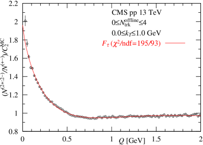
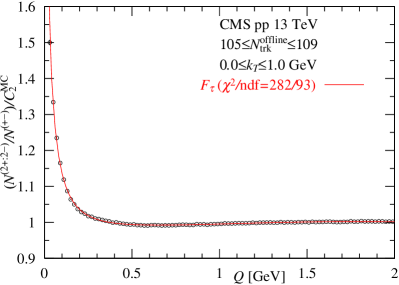
Figure 1: Fit to the BEC measurements by CMS in pp collisions at 13 TeV by Eq. (1). $C_{2}^{MC}\equiv N_{\rm MC}^{(2+:2-)}/N_{\rm MC}^{(+-)}$, where $N_{\rm MC}$’s mean the numbers of the same charged and opposite charged pairs recorded in MC simulations.

Table 1: Fit parameters to the CMS BEC measurements in pp collisions at 13 TeV at $0.0\leq k_{T}\leq 1.0$ GeV by Eq. (1). $\delta$ values are estimated (top to bottom): $-0.016\pm 0.004$, $0.03\pm 0.01$, $0.005\pm 0.005$, $(-1.2\pm 0.1)\times 10^{-3}$, $(1.3\pm 0.2)\times 10^{-3}$, and $0.002\pm 0.001$.

$N_{\rm trk}^{\rm offline}$	$r_{0}$ (fm)	$r$ (fm)	$\lambda$	$\alpha_{\tau}$	$\chi^{2}$/ndf	$\chi^{2}$(CMS)
$0-4$	$0.139\pm 0.021$	$0.93\pm 0.06$	$0.96\pm 0.05$	$0.781\pm 0.026$	195/93	195
$10-12$	$0.244\pm 0.004$	$9.08\pm 1.40$	$2.43\pm 0.23$	$0.420\pm 0.013$	140/93	140
$31-33$	$0.232\pm 0.005$	$21.8\pm 4.0$	$3.36\pm 0.37$	$0.377\pm 0.011$	135/93	135
$80-84$	$0.224\pm 0.001$	$43.7\pm 2.5$	$4.48\pm 0.15$	$0.351\pm 0.003$	899/93	902
$105-109$	$0.216\pm 0.003$	$47.0\pm 5.2$	$4.71\pm 0.31$	$0.352\pm 0.005$	282/93	281
$130-250$	$0.228\pm 0.013$	$53.3\pm 19.9$	$5.32\pm 1.27$	$0.353\pm 0.020$	84.5/93	84

Because estimated values of all parameters by $\tau$-model, i.e., Eq. (1), have not been presented in Ref. [1], it is difficult to draw physical picture through the analyses of BEC in pp collisions at 13 TeV. Thus for this aim, we present them in Table 1. Table 1 shows that the $\chi^{2}/$ndf values obtained from our analysis are consistent with those reported by the CMS Collaboration [1]. In other words, through concrete figures in Table 1, we are able to consider physical picture based on the $\tau$-model.

As indicated in Table 1, the interaction ranges of the Levy-type form ($e^{-(Qr)^{\alpha}}$) increase as the interval containing $N_{\rm trk}^{\rm offline}$ increases. The estimated values $r=20\sim 50$ fm appear large for pp collisions at 13 TeV.

This paper also investigates this issue from a different perspective, focusing on the collision mechanism. Three processes occur in collisions at the LHC [5, 6, 7]: the non-diffractive dissociation, the single-diffractive dissociation, and the double-diffractive dissociation (DD). BEC are related to the chaotic components of particle production. Since the contribution from the DD is Poissonian [7], there is no effect to the BEC. Thus we calculated the following two-component model correlation function [7, 8] (see also empirical Refs. [9, 10, 11]),

$${\rm CF_{II}}=1+\lambda_{1}E_{\rm BE_{1}}+\lambda_{2}E_{\rm BE_{2}}.$$ (2)

The exchange function is the Fourier transform of the space-time region emitting bosons (mainly pion) with overlapping wave functions. For the exchange functions $E_{\rm BE_{1}}$ and $E_{\rm BE_{2}}$, we assign the following two functions [12],

$$\exp(-R_{1}Q)\quad{\rm and}\quad\exp\left(-(R_{2}Q)^{2}\right)$$ (3)

characterizing the exponential and Gaussian type of BEC. Thus $R_{1}$ and $R_{2}$ mean the extensions of the sources [12]. Concerning with two kinds of exchange functions, see also the different approach[13].

Moreover, we discuss the LRC’s below. Three decades ago, the OPAL Collaboration [14] adopted LRC${}_{(\rm OPAL)}=c(1+\delta Q+\varepsilon Q^{2})$ to improve the linear form LRC${}_{(\rm linear)}=C(1+\delta Q)$. Recently we proposed the inverse power series form LRC${}_{(\rm p.s.)}=C/[1-\alpha Q\exp(\beta Q)]$ [15], because the number of parameters ($\alpha$ and $\beta$) is the same as the LRC_(OPAL)’s, and it converges to $C$ as $Q$ is large. Taking into account of those investigations and mathematical descriptions shown in Ref. [1], i.e., the distribution of opposite charged pion pair $N^{(+-)}=C[1+a\exp{(-bQ^{2})}]$ and so on, we propose the following form:

$${\rm LRC_{(Gauss)}}=\frac{C}{1.0+\alpha\exp(-\beta Q^{2})}.$$ (4)

This function converges to $C$ as $Q$ is large and behaves as $C[1-\alpha(1-\beta Q^{2})+\cdots]$, $Q$ being small. In Table 2, we compare our approach with formulas shown in Ref. [1].

Table 2: Comparison of our approach with formulas utilized by CMS Collaboration [1].

	formulas	cf.
	${\rm CF_{II}\times LRC}$	1) ${\rm CF_{II}}$ is reflecting to three kinds of multiplicity
Our	where	distributions of the ND, SD, and DD in pp collisions.
approach	${\rm LRC_{(Exp)}}=\dfrac{1}{1+\alpha e^{-\beta Q}}$,	2) Through the generalization of ${\rm LRC_{(OPAL)}}$
	or	$=1+\delta Q+\varepsilon Q^{2}$ in e+e- annihilation at Z0-pole [14],
	${\rm LRC_{(Gauss)}}=\dfrac{1}{1+\alpha e^{-\beta Q^{2}}}$.	we obtained ${\rm LRC_{(Exp)}}$ [15].
		3) Referring to mathematical descriptions on $F_{2N}$ and
		$F_{2D}$ in Ref [1], ${\rm LRC_{(Gauss)}}$ is proposed for pp collisions.
	1) Distributions $N^{(2+:2-)}$, $N^{(+-)}$,	1) ${\rm CF_{I}}=1+\lambda E_{\rm BE}$, where $E_{\rm BE}=\exp(-RQ)$ [1].
CMS	$N_{\rm MC}^{(2+:2-)}$ and $N_{\rm MC}^{(+-)}$ are assumed	2) Provided that $N_{\rm MC}^{(+-)}\cong N^{(+-)}$ and the cross term
	as follows: ${\rm CF_{I}}\cdot C(1+ae^{-bQ^{2}})$,	($\lambda aE_{\rm BE}\cdot e^{-bQ^{2}}$) is small, we obtain
	$C^{\prime}(1+a^{\prime}e^{-b^{\prime}Q^{2}})$, $C_{M}(1+a_{M}e^{-b_{M}Q^{2}})$	$\dfrac{F_{2N}}{F_{2D}}\cong\dfrac{{\rm CF_{I}}\times(1+ae^{-bQ^{2}})}{1+a_{M}e^{-b_{M}Q^{2}}}\cong{\rm CF_{II}\times LRC_{(Gauss)}}$.
	and $C_{M}^{\prime}(1+a_{M}^{\prime}e^{-b_{M}^{\prime}Q^{2}})$, respectively.	Thus, $\alpha$ and $\beta$ in Eq. (4) are approximately identified
	2) SR’s $F_{2N}=N^{(2+:2-)}/N^{(+-)}$ and	with $a_{M}$ and $b_{M}$ describing the Monte Carlo events
	$F_{2D}=N_{\rm MC}^{(2+:2-)}/N_{\rm MC}^{(+-)}$ are used for	in $F_{2D}$, respectively.
	analysis of data of DR by the ratio	3) Their Monte Carlo events are calculated by
	$F_{2N}/F_{2D}$.	PYTHIA6. See Fig. 3 in Ref. [2].
	3) $\tau$-model is also used for data of DR.

In the second section, we analyze the BEC at 13 TeV using Eqs. (2)–(4). In the third section, we present our predictions for 3-pion BEC using the two-component model. In the final section, we provide concluding remarks. Appendix A presents an analysis of BEC at 13 TeV using the $\tau$-model with Eq. (4). In Appendix B, we reanalyze the CMS BEC at 0.9 and 7 TeV utilizing Eq. (4), because in previous works [7, 8], we used LRC${}_{(\rm linear)}=C(1+\delta Q)$.

2 Analysis of BEC at 13 TeV using Eqs. (2)–(4).

Considering the results of the CMS BEC at 7 TeV in Ref. [7], we assume a combination of exponential function and Gaussian distribution, as this combination has shown the valuable role. Moreover, it is worthwhile to mention that Shimoda et al. in Ref. [12] investigated several possible distributions for $E_{\rm BE}$’s. Our results are presented in Fig. 2 and Table 3. We observe extraordinary behaviors in the two intervals, $0\leq N_{\rm trk}^{\rm offline}\leq 4$ and $10\leq N_{\rm trk}^{\rm offline}\leq 12$, of the LRC shown in Fig. 3.

As indicated by Fig. 2 and Table 3, the two-component model with Eqs. (2)–(4) effectively characterizes three intervals: $31\leq N_{\rm trk}^{\rm offline}\leq 33$, $80\leq N_{\rm trk}^{\rm offline}\leq 84$, and $105\leq N_{\rm trk}^{\rm offline}\leq 109$.

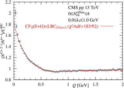
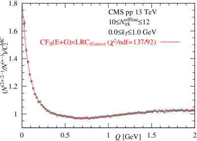
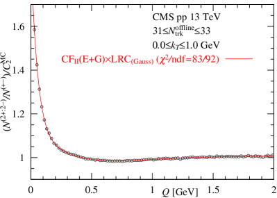
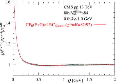
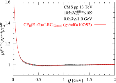
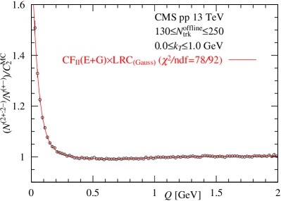
Figure 2: Fit to the BEC measurements by CMS in pp collisions at 13 TeV by Eqs. (2)–(4).

Table 3: Fit parameters of the CMS measurements of BEC in pp collisions at 13 TeV ($0.0\leq k_{T}\leq 1.0$ GeV) by Eqs. (2)–(4). Three constraints are used: $\lambda_{1}\leq 1.0$, $\lambda_{2}\leq 1.0$, and $\lambda_{1}+\lambda_{2}\leq 1.0$. The $p$-values for the three intervals $31\leq N_{\rm trk}^{\rm offline}\leq 33$, $80\leq N_{\rm trk}^{\rm offline}\leq 84$, and $130\leq N_{\rm trk}^{\rm offline}\leq 250$ are 73.0 %, 77.3 % and 85.3 %, respectively. $C$ (top to bottom): $0.980\pm 0.004$, $1.031\pm 0.001$, $1.007\pm 0.001$, $1.001\pm 1\times 10^{-4}$, $1.003\pm 2\times 10^{-4}$, $1.003\pm 0.001$, $0.972\pm 0.002$, $1.028\pm 0.002$, and $1.007\pm 0.001$.

$N_{\rm trk}^{\rm offline}$	$R_{1}$ (fm)	$R_{2}$ (fm)	$\lambda_{1}$	$\lambda_{2}$	$\alpha$	$\beta$ (GeV-2)	$\chi^{2}$/ndf
$0-4$	$1.57\pm 0.15$	$0.51\pm 0.01$	$0.680\pm 0.034$	$0.320\pm 0.034$	$0.062\pm 0.006$	$0.79\pm 0.18$	185.4/92
$10-12$	$2.40\pm 0.07$	$0.39\pm 0.02$	$0.865\pm 0.007$	$0.135\pm 0.007$	$0.136\pm 0.009$	$0.99\pm 0.07$	137.1/92
$31-33$	$3.37\pm 0.07$	$0.48\pm 0.02$	$0.910\pm 0.004$	$0.090\pm 0.004$	$0.048\pm 0.004$	$1.06\pm 0.12$	83.3/92
$80-84$	$3.76\pm 0.03$	$0.49\pm 0.01$	$0.866\pm 0.007$	$0.061\pm 0.001$	$0.026\pm 0.001$	$1.53\pm 0.06$	81.6/92
$105-109$	$4.02\pm 0.06$	$0.57\pm 0.01$	$0.867\pm 0.149$	$0.050\pm 0.002$	$0.020\pm 0.001$	$1.06\pm 0.07$	107.0/92
$130-250$	$3.79\pm 0.22$	$0.46\pm 0.09$	$0.857\pm 0.051$	$0.040\pm 0.011$	$0.030\pm 0.014$	$1.54\pm 0.51$	77.6/92
Note: When no constraint is applied for $\lambda_{1}$ and $\lambda_{2}$, we obtain the following figures:
$0-4$	$2.76\pm 0.30$	$0.49\pm 0.02$	$1.085\pm 0.083$	$0.477\pm 0.052$	$0.112\pm 0.051$	$1.78\pm 0.57$	126.6/92
$10-12$	$2.50\pm 0.09$	$0.37\pm 0.02$	$0.947\pm 0.033$	$0.168\pm 0.025$	$0.165\pm 0.028$	$1.17\pm 0.13$	128.8/92
$31-33$	$3.43\pm 0.11$	$0.48\pm 0.02$	$0.928\pm 0.029$	$0.092\pm 0.004$	$0.048\pm 0.004$	$1.06\pm 0.12$	83.0/92

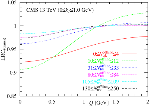
Figure 3: The long-range correlations (LRCs), see Eq. (4) for six intervals.

Among the six intervals shown in Fig. 3, the red (solid) line and green (dashed) line appear to be exceptional. They are probably related to the normalization factors ($0.980\pm 0.004$ and $1.031\pm 0.001$). In other words, in those regions there is very small freedom or noise which cannot be described by Eqs. (2)–(4).

3 Test of the two-component model for 3-pion BEC

Here, we investigate the 3-pion BEC using the two-component model. Since there is currently no information from CMS on the multiplicity distribution $P(n)$ at 13 TeV, it is challenging to determine the ratio between the contributions of the first and the second components. We use the diagrams in Fig. 4.

Figure 4: Diagrams for the third-order BEC. The matrix indicates the exchange of identical pions.

The formula that corresponds to the diagrams in Fig. 4 [16, 17, 18] is expressed as

$$F_{i}^{(3)}=1.0+3\lambda_{i}E_{\rm BE_{i}}+2(\lambda_{i}E_{\rm BE_{i}})^{3/2}$$ (5)

By assuming an equal weight for the first and the second components, $F_{1}^{(3)}$ and $F_{2}^{(3)}$, we obtain the following normalized expression

$$F^{(3+:3-)}=1.0+\frac{1}{2}\left(3\lambda_{1}E_{\rm BE_{1}}+2(\lambda_{1}E_{\rm BE_{1}})^{3/2}\right)+\frac{1}{2}\left(3\lambda_{2}E_{\rm BE_{2}}+2(\lambda_{2}E_{\rm BE_{2}})^{3/2}\right),$$ (6)

where $\lambda_{1}$, $\lambda_{2}$, $R_{1}$, and $R_{2}$ are fixed by using the numerical values in Table3. Typical figures are presented in Fig. 5. We could calculate the ratio if the CMS Collaboration reports the multiplicity distributions $P(n)$ [2], as this would allow us to understand the ensemble property of the BEC through the multiplicity distribution. It is worth noting that the ATLAS Collaboration has already observed the multiplicity distributions $P(n)$ [19] and BEC [20] to be considered in [21].

Figure 5: Prediction of upper limit of the 3$\pi$ BEC in pp collisions at 13 TeV by means of Eq. (6) with Eqs. (2)-(4). $N^{\rm(BG)}$ means $N_{\rm MC}^{(3+:3-)}$, because of no-BEC in the Monte Carlo events.

In the near future, we may be able to further test the two-component model when the CMS Collaboration analyzes the 3-$\pi$ BEC. If we observe the same extensions as in Fig. 2, we could conclude that the two-component model is a viable approach.

4 Concluding remarks

C1)

Our analysis of CMS BEC at 13 TeV using the $\tau$-model with Eq. (1) confirms the applicability of this model. This is evidenced by the values of $\chi^{2}$ in Table 1.

C2)

As portrayed in Table 1, the interaction ranges $r$ in the Lévy-type expression $e^{-(Qr)^{\alpha_{\tau}}}$ increase as the range of the interval $N_{\rm trk}^{\rm offline}$ increases. However, it appears that the interaction ranges from 30 to 50 fm are large in $pp$ collisions at 13 TeV.

C3)

To gain a better understanding of the results obtained from the $\tau$-model, we have analyzed the BEC using the $\tau$-model with Eq. (4). This has led to improved estimations, as shown in Appendix A.

C4)

We look forward to future analyses by the CMS Collaboration of the multiplicity distributions and the third-order BEC at 13 TeV

Hereafter, we summarize the results of the two-component model using Eqs. (2)–(4).

C5)

In Table 2, we mentioned how to propose LRC_(Gauss), i.e., Eq. (4). To investigate the remarks mentioned in C2) above using the two-component model, we utilized Eqs. (2)–(4). Our results are presented in Table 3. The large extensions are approximately 4 fm, and they appear to be reasonable.

C6)

Furthermore, to test the availability of the two-component model, we calculated the 3-pion BEC by making use of the estimated values and diagrams presented in Fig. 4. Interestingly, as $N_{\rm trk}^{\rm offline}$ increases, the 3-pion BEC rapidly decreases, due to the changes in the extension $R_{1}$ (1 fm to 4 fm). Moreover, the intercepts at $Q=0.0$ GeV are about 3.0, providing the equal weight.

C7)

To investigate the role of the LRC_(Gauss), i.e., Eq. (4), we reanalyzed the BEC at 0.9 and 7 TeV, with the results presented in Appendix B. The estimated $\chi^{2}$ values became smaller than that of LRC_(linear) [7]. We also analyzed the data with the constraint, $0.1\leq k_{T}\leq 0.3$ GeV and $2\leq N_{\rm ch}\leq 9$. We observe that $R_{1}$’s increase and $R_{2}$’s are almost constant.

C8)

As portrayed in Table 3, the BEC in the intervals $0\leq N_{\rm trk}^{\rm offline}\leq 4$ and $10\leq N_{\rm trk}^{\rm offline}\leq 12$ cannot be analyzed with better $\chi^{2}$ values. A more complicated model may be necessary.

C9)

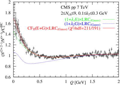
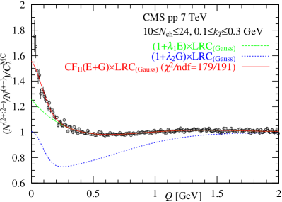
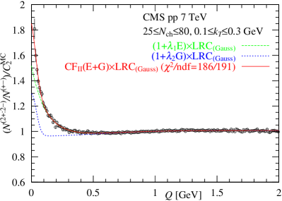
Figure 11: Fit to the BEC measurements by CMS in pp collisions at 7 TeV with $0.1\leq k_{T}\leq 0.3$ GeV by Eqs. (2)–(4).

From Table 3, we can observe behaviors of $R_{1}$ and $R_{2}$’s in Fig. 6. The larger extension $R_{1}$’s seem to be saturated at larger $N_{\rm trk}^{\rm offline}$. To confirm that, of course, more data are needed. Compare Fig. 11 and Table 6 in Appendix B, where data at 7 TeV with the constraints $0.1\leq k_{T}\leq 0.3$ GeV and and $2\leq N_{\rm ch}\leq 9$ are analyzed. See also discussions on two kinds of extensions mentioned in Ref. [13].

Figure 6: Behaviors of $R_{1}$ and $R_{2}$’s estimated in Table 3. The smaller extension $R_{2}$’s are almost the constant.

Acknowledgments. One of the authors (M.B.) would like to thank his colleagues at the Department of Physics, Shinshu University.

Appendix A Analysis of BEC at 13 TeV using the $\tau$-model with Eq. (4)

We are interested in the influence of Eq. (4) on the $\tau$-model. To investigate this, we reanalyzed the BEC using the following formula

$$F_{\tau\mathchar 45\relax{\rm Gauss}}=[1+\lambda\cos((r_{0}Q)^{2}+\tan(\alpha_{\tau}\pi/4)(Qr)^{\alpha_{\tau}})e^{-(Qr)^{\alpha_{\tau}}}]\cdot{\rm LRC_{(Gauss)}}$$ (7)

Our findings are presented in Fig. 7 and Table 4. It can be seen that the interaction range $r$ values are smaller than 10 fm.

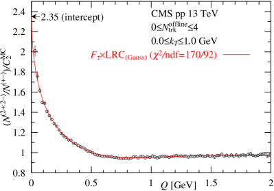
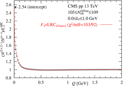
Figure 7: Fit to the BEC measurements by CMS in pp collisions at 13 TeV by Eq. (7) with Eq. (4).

Table 4: Fit parameters of the CMS measurements of BEC in pp collisions at 13 TeV ($0.0\leq k_{T}\leq 1.0$ GeV) using the $\tau$-model with Eq. (4).

$N_{\rm trk}^{\rm offline}$	$r_{0}$ (fm)	$r$ (fm)	$\lambda$	$\alpha_{\tau}$	$\alpha$	$\beta$	$\chi^{2}$/ndf
$0-4$	$0.22\pm 0.02$	$2.12\pm 0.52$	$1.02\pm 0.12$	$0.595\pm 0.047$	$\!\!\!\!-0.169\pm 0.017$	$5.60\pm 0.49$	169.6/92
$10-12$	$0.25\pm 0.01$	$9.89\pm 1.69$	$2.49\pm 0.25$	$0.417\pm 0.014$	$0.099\pm 0.060$	$0.17\pm 0.13$	138.7/92
$31-33$	$0.16\pm 0.01$	$3.27\pm 0.45$	$1.76\pm 0.10$	$0.566\pm 0.022$	$0.177\pm 0.024$	$19.86\pm 1.02$	85.9/92
$80-84$	$0.00$	$3.76\pm 0.06$	$1.65\pm 0.02$	$0.566\pm 0.002$	$0.159\pm 0.003$	$23.83\pm 0.31$	166.2/92
$105-109$	$0.13\pm 0.01$	$5.61\pm 0.54$	$1.84\pm 0.08$	$0.517\pm 0.012$	$0.119\pm 0.010$	$25.48\pm 0.73$	103.1/92
$130-250$	$0.18\pm 0.02$	$9.02\pm 3.43$	$2.18\pm 0.42$	$0.468\pm 0.037$	$0.076\pm 0.024$	$21.63\pm 3.39$	78.5/92

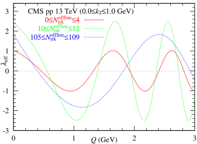
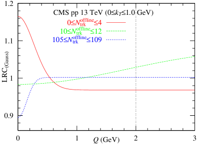
Figure 8: $\lambda_{\rm eff}$’s and LRCs of BEC measurements by CMS in pp collisions at 13 TeV by Eq. (7). The vertical line at $Q=2.0$ GeV represents the effective range of the LRC ($0\leq Q\leq 2$ GeV).

As illustrated in Fig. 8, three LRC’s appear to be various. Therein the behavior of LRC for $0\leq N_{\rm trk}^{\rm offline}\leq 4$ is related to the negative $\alpha$. For the sake of reference, we demonstrate the effective degree of coherence in the $\tau$-model,

$$\lambda_{\rm eff}=\lambda\cos((r_{0}Q)^{2}+\tan(\alpha_{\tau}\pi/4)(Qr)^{\alpha_{\tau}})$$

in Fig. 8. By making use of $\lambda_{\rm eff}$’s and LRCs, we can estimate the intercepts at $Q=0.0$ GeV, which are shown in Fig. 7.

Appendix B Reanalysis of CMS BEC at 0.9 and 7 TeV [2] by LRC, expressed by Eq. (4)

We examined the changes in the values of $\chi^{2}$ when LRC_(linear) was replaced with Eq. (4) in the reanalysis of BEC at 0.9 and 7 TeV [2]. Our new results obtained using Eq. (4) are presented in Fig. 9 and Table 5 and compared with those obtained elsewhere [7], where the linear form for the ${\rm LRC}=C(1+\delta Q)$ was used. These results are also shown in Table 5. We show the LRCs in Fig. 10.

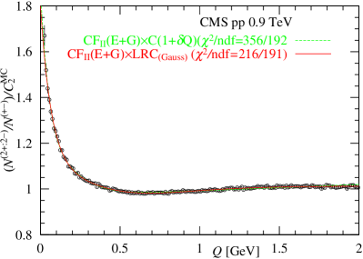
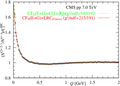
Figure 9: Fit to the CMS BEC measurements in pp collisions at 0.9 and 7.0 TeV by Eqs. (2)–(4).

Table 5: Fit parameters of the CMS BEC measurements in pp collisions at 0.9 and 7.0 TeV by Eqs. (2)–(4).

	$R_{1}$ (fm)	$R_{2}$ (fm)	$\lambda_{1}$	$\lambda_{2}$	$\!\!\!\delta\,({\rm GeV}^{-1})$ or $(\alpha,\ \beta\,({\rm GeV}^{-2}))\!\!\!$	$\chi^{2}$/ndf
$\sqrt{s}=0.9$ TeV
LRC(linear) [7]	$1.42\pm 0.03$	$3.37\pm 0.42$	$0.53\pm 0.02$	$0.23\pm 0.04$	$0.030\pm 0.001$	417/192
Eq. (4)	$0.82\pm 0.10$	$2.27\pm 0.13$	$0.41\pm 0.01$	$0.30\pm 0.02$	$(0.10\pm 0.02,\ 1.38\pm 0.10)$	234/191
$\sqrt{s}=7$ TeV
LRC(linear) [7]	$3.88\pm 0.18$	$0.71\pm 0.01$	$0.84\pm 0.03$	$0.12\pm 0.01$	$0.023\pm 0.001$	540/192
Eq. (4)	$3.13\pm 0.13$	$0.51\pm 0.02$	$0.80\pm 0.03$	$0.10\pm 0.01$	$(0.06\pm 0.01,\ 1.46\pm 0.11)$	217/191

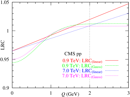
Figure 10: LRCs by LRC_(linear) [7] and LRC_(Gauss) (Eq. (4)) of CMS BEC measurements in pp collisions at 0.9 and 7.0 TeV are presented. The vertical line at $Q=2.0$ GeV represents the effective range of the LRC ($0\leq Q\leq 2$ GeV).

It can be said that the Gaussian distribution of the LRC in the two-component model is better than that of the linear form, because the LRC_(Gauss) converges to 1.0 in the region $Q\geq 2.0$ GeV. The reason is as follows: The emitting source functions and/or the LRC’s in the Euclidean space ($Q^{\prime}=\sqrt{({\bf p}_{1}-{\bf p}_{2})^{2}+(E_{1}-E_{2})^{2}}$ and $\xi^{\prime}=\sqrt{({\bf r}_{1}-{\bf r}_{2})^{2}+(t_{1}-t_{2})^{2}}$) are calculated as

$$F_{\rm source}(\xi^{\prime},\,R)=\frac{1}{(2\pi)^{2}\xi^{\prime}}\int_{0}^{\infty}Q^{\prime 2}\,E_{\rm BE}(Q^{\prime},\,R)\,J_{1}(Q^{\prime}\xi^{\prime})dQ^{\prime}$$ (8)

where $J_{1}(Q\xi)$ is the Bessel function. For the LRC, we should replace $E_{\rm BE}$ with (LRC$-1.0$) and $R$ with $\beta$ in Eq. (8), respectively. In other words, the $({\rm LRC_{(Gauss)}-1.0})=\sum_{k=1}^{\infty}(-\alpha e^{-\beta Q^{2}})^{k}$ is preferable to the $({\rm LRC_{(linear)}-1.0)}=\delta Q$, because the former converges, as $Q$ is large. Finally, we should adopt the inverse Wick rotation for $\xi^{\prime}$ [12, 15]; $\xi=\sqrt{({\bf r}_{1}-{\bf r}_{2})^{2}-(t_{1}-t_{2})^{2}}$.

Finally we analyzed data on BEC at 7 TeV with $0.1\leq k_{T}\leq 0.3$ GeV and $2\leq N_{\rm ch}\leq 9$ in Ref. [2] by means of Eqs. (2)-(4). The smaller extensions are almost constant. This fact is similar to Fig. 6. From estimated parameters with the constraint $2\leq N_{\rm ch}\leq 9$ (fixed), we know that both $R_{1}$ and $R_{2}$’s are approximately constant.

Table 6: Fit parameters of the CMS BEC measurements in pp collisions at 7.0 TeV with $0.1\leq k_{T}\leq 0.3$ GeV and $2\leq N_{\rm ch}\leq 9$ by Eqs. (2)–(4) with $0\leq\lambda_{1}\leq 1$ and $\lambda_{2}=1-\lambda_{1}$. $N_{\rm ch}$ means the charged particle multiplicity. $C$ (top to bottom): $1.037\pm 0.011$, $1.013\pm 0.001$, $1.008\pm 0.001$, $1.010\pm 0.008$, and $1.037\pm 0.011$.

	$R_{1}$(fm)	$R_{2}$(fm)	$\lambda_{1}$	$\lambda_{2}$	$\alpha$	$\beta$ (GeV-2)	$\chi^{2}$/ndf
$0.1\leq k_{T}\leq 0.3$ (fixed)
$2\leq N_{\rm ch}\leq 9$	$1.16\pm 0.31$	$0.36\pm 0.19$	$0.95\pm 0.10$	$0.05\pm 0.10$	$0.14\pm 0.04$	$0.80\pm 0.28$	212/192
$10\leq N_{\rm ch}\leq 24$	$2.05\pm 0.25$	$0.46\pm 0.04$	$0.95\pm 0.10$	$0.05\pm 0.10$	$0.14\pm 0.03$	$2.42\pm 0.24$	188/192
$25\leq N_{\rm ch}\leq 80$	$2.77\pm 0.14$	$0.47\pm 0.04$	$0.91\pm 0.02$	$0.09\pm 0.02$	$0.08\pm 0.02$	$2.47\pm 0.26$	176/192
$2\leq N_{\rm ch}\leq 9$ (fixed)
$0.1\leq k_{T}\leq 0.3$	$1.16\pm 0.31$	$0.36\pm 0.19$	$0.95\pm 0.10$	$0.05\pm 0.10$	$0.14\pm 0.04$	$0.80\pm 0.28$	212/192
$0.3\leq k_{T}\leq 0.5$	$1.47\pm 0.20$	$0.29\pm 0.05$	$0.86\pm 0.03$	$0.14\pm 0.03$	$0.15\pm 0.04$	$0.99\pm 0.23$	198/192
$0.5\leq k_{T}\leq 1.0$	$0.97\pm 0.41$	$0.25\pm 0.07$	$0.71\pm 0.10$	$0.29\pm 0.10$	$0.43\pm 0.08$	$1.16\pm 0.32$	177/192

References

• [1] A. M. Sirunyan et al. [CMS], JHEP 03 (2020), 014.
• [2] V. Khachatryan et al. [CMS], JHEP 05 (2011), 029.
• [3] H. Takayasu, “Fractals in the Physical Sciences,” Manchester University Press, 1990.
• [4] K. Itô, “Kakuritsu Katei” (Translation from the English language edition, “Stochastic Processes”), Springer-Verlag, Berlin Heidelberg, 2004.
• [5] S. Navin, “Diffraction in ALICE and trigger efficiencies,” CERN-THESIS-2011-378.
• [6] I. Zborovský, J. Phys. G 40 (2013), 055005.
• [7] M. Biyajima and T. Mizoguchi, Int. J. Mod. Phys. A 34 (2019) no.31, 1950203.
• [8] T. Mizoguchi and M. Biyajima, JPS Conf. Proc. 26 (2019), 031032.
• [9] T. Åkesson et al. [Axial Field Spectrometer], Z. Phys. C 36 (1987), 517.
• [10] N. M. Agababyan et al. [EHS/NA22], Z. Phys. C 59 (1993), 195-210.
• [11] B. Lorstad, Int. J. Mod. Phys. A 4 (1989), 2861-2896.
• [12] R. Shimoda, M. Biyajima and N. Suzuki, Prog. Theor. Phys. 89 (1993), 697-708.
• [13] V. A. Khoze, A. D. Martin, M. G. Ryskin and V. A. Schegelsky, Eur. Phys. J. C 76 (2016) no.4, 193.
• [14] P. D. Acton et al. [OPAL Collaboration], Phys. Lett. B 267 (1991) 143.
• [15] T. Mizoguchi, S. Matsumoto and M. Biyajima, Int. J. Mod. Phys. A 37 (2022) no.25, 2250148.
• [16] M. Biyajima, A. Bartl, T. Mizoguchi, O. Terazawa and N. Suzuki, Prog. Theor. Phys. 84 (1990), 931-940; See also ibid 88 (1992), 157.
• [17] N. Suzuki and M. Biyajima, Phys. Rev. C 60 (1999), 034903.
• [18] G. A. Kozlov, O. V. Utyuzh, G. Wilk and Z. Wlodarczyk, Phys. Atom. Nucl. 71 (2008), 1502-1504.
• [19] M. Aaboud et al. [ATLAS], Eur. Phys. J. C 76 (2016) no.9, 502.
• [20] G. Aad et al. [ATLAS], Eur. Phys. J. C 82 (2022) no.7, 608.
• [21] M. Biyajima, T. Mizoguchi, and S. Matsumoto in preparation.