Change Point Detection on A Separable Model
for Dynamic Networks

Abstract

This paper studies change point detection in time series of networks, with the Separable Temporal Exponential-family Random Graph Model (STERGM). Dynamic network patterns can be inherently complex due to dyadic and temporal dependence. Detection of the change points can identify the discrepancies in the underlying data generating processes and facilitate downstream analysis. The STERGM that utilizes network statistics to represent the structural patterns is a flexible model to fit dynamic networks. We propose a new estimator derived from the Alternating Direction Method of Multipliers (ADMM) and Group Fused Lasso to simultaneously detect multiple time points, where the parameters of a time-heterogeneous STERGM have changed. We also provide a Bayesian information criterion for model selection and an R package CPDstergm to implement the proposed method. Experiments on simulated and real data show good performance of the proposed framework.

Keywords: Change Point Detection, Dynamic Networks, Alternating Direction Method of Multipliers, Group Fused Lasso, Temporal Exponential-family Random Graph Model

1 Introduction

Networks are often used to describe relational phenomena that cannot be limited merely to the attributes of individuals. In an investigation of the transmission of COVID-19, Fritz et al. (2021) used networks to represent human mobility and forecast disease incidents. The study of physical connections, beyond the health status of individuals, permits policymakers to implement preventive measures effectively and allocate healthcare resources efficiently. Yet relations can change over time, and dynamic relational phenomena are often aggregated into a static network for analysis. To this end, a temporal model for dynamic networks is in high demand.

In recent decades, a plethora of models has been proposed for dynamic networks analysis. Snijders (2001), Snijders (2005), and Snijders et al. (2010) developed a Stochastic Actor-Oriented Model, which is driven by the actor’s perspective to make or withdraw ties to other actors in a network. Kolar et al. (2010) focused on recovering the latent time-varying graph structures of Markov Random Fields, from serial observations of nodal attributes. Sarkar and Moore (2005), Sewell and Chen (2015), and Sewell and Chen (2016) presented a Latent Space Model, by assuming the edges between actors are more likely when they are closer in the latent Euclidean space. Matias and Miele (2017), Ludkin et al. (2018), and Pensky (2019) investigated the dynamic Stochastic Block Model (SBM), and Jiang et al. (2020) developed an Autoregressive SBM to characterize the communities. Furthermore, the Exponential-family Random Graph Model (ERGM) that uses local forces to shape global structures (Hunter et al., 2008b) is a promising model for networks with dependent ties. Hanneke et al. (2010) defined a Temporal ERGM (TERGM), by conditioning on previous networks in the network statistics of an ERGM. Desmarais and Cranmer (2012b) proposed a bootstrap approach to maximize the pseudo-likelihood of the TERGM and assess uncertainty. In general, network evolution concerns the rate at which edges form and dissolve. Demonstrated in Krivitsky and Handcock (2014), these two factors can be mutually interfering, making the dynamic models used in the literature difficult to interpret. Posing that the underlying reasons that result in dyad formation are different from those that result in dyad dissolution, Krivitsky and Handcock (2014) proposed a Separable TERGM (STERGM) to dissect the entanglement with two conditionally independent models.

In time series analysis, change point detection plays a central role in identifying the discrepancies in the underlying data generating processes. Without taking the structural changes across dynamic networks into consideration, learning from the time series may not be meaningful. As relational phenomena are studied in numerous domains, it is practical for researcher to first localize the change points, and then analyze the dynamic networks, rather than overlooking where the network patterns have substantially changed.

There has also been an increasing interest in studying the change point detection problem for dynamic networks. Wang et al. (2013) focused on the Stochastic Block Model time series, and Wang et al. (2021) studied a sequence of inhomogeneous Bernoulli networks. Larroca et al. (2021), Marenco et al. (2022), and Padilla et al. (2022) considered a sequence of Random Dot Product Graphs that are both dyadic and temporal dependent. Methodologically, Chen and Zhang (2015), and Chu and Chen (2019) developed a graph-based approach to delineate the distributional differences before and after a change point, and Chen (2019) utilized the nearest neighbor information to detect the changes in an online framework. Zhao et al. (2019) proposed a two-step approach that consists of an initial graphon estimation followed by a screening algorithm, Song and Chen (2022b) exploited the features in high dimensions via a kernel-based method, and Chen et al. (2020a) employed embedding methods to detect both anomalous graphs and anomalous vertices. Moreover, Liu et al. (2018) introduced an eigenvector-based method to reveal the change and persistence in the gene communities for a developing brain. Bybee and Atchadé (2018) focused on a Gaussian Graphical Model to detect the change points in the covariance structure of the Standard and Poor’s 500. Ondrus et al. (2021) proposed a factorized binary search method to understand brain connectivity from the functional Magnetic Resonance Imaging time series data.

Allowing for user-specified network statistics to determine the structural changes for the detection, we make the following contributions in the proposed framework:

• To simultaneously detect multiple change points from a sequence of networks, we learn a time-heterogeneous STERGM, while penalizing the sum of Euclidean norms of the sequential parameter differences. We formulate the augmented Lagrangian as a Group Fused Lasso problem, and we derive an Alternating Direction Method of Multipliers (ADMM) to solve the optimization problem.

• We exploit the practicality of STERGM, which manages dyad formation and dissolution separately, to capture the structural changes in network evolution. The flexibility of STERGM, which considers both dyadic and temporal dependence, and the extensive selection of network statistics also boost the power of the proposed method. Moreover, we provide a Bayesian information criterion for model selection, and we develop an R package CPDstergm to implement the proposed method.

• We simulate dynamic networks to imitate realistic social interactions, and our method can achieve greater accuracy on the networks that are both dyadic and temporal dependent. Furthermore, we punctually detect the winter and spring vacations with the MIT cellphone data (Eagle and Pentland, 2006). We also detect three major change points from the stock market data analyzed in James and Matteson (2015), and the detected change points align with three significant events during the 2008 worldwide economic crisis.

The rest of the paper is organized as follows. In Section 2, we review the STERGM for dynamic networks. In Section 3, we present the likelihood-based objective function with Group Fused Lasso regularization, and we derive an ADMM to solve the optimization problem. In Section 4, we discuss change points localization after parameter learning, along with model selection and post-processing. In Section 5, we implement our method on simulated and real data. In Section 6, we conclude our work with a discussion and potential future developments.

2 STERGM Change Point Model

2.1 Notation

For a matrix $\bm{X}\in\mathbb{R}^{\tau\times p}$, denote $\bm{X}_{i,\bm{\cdot}}\in\mathbb{R}^{1\times p}$ and $\bm{X}_{\bm{\cdot},i}\in\mathbb{R}^{\tau\times 1}$ as the respective $i$th row and $i$th column of the matrix $\bm{X}$. Moreover, denote $\bm{X}_{-i,\bm{\cdot}}\in\mathbb{R}^{\tau\times p}$ as the matrix obtained by replacing the $i$th row of the matrix $\bm{X}$ with a zero vector, and $\bm{X}_{\bm{\cdot},-i}\in\mathbb{R}^{\tau\times p}$ is denoted similarly.

For a matrix $\bm{\theta}\in\mathbb{R}^{\tau\times p}$, define the transformation from a matrix to a vector as $\vv{\bm{\theta}}=\text{vec}_{\tau p}(\bm{\theta})\in\mathbb{R}^{\tau p\times 1}$, by sequentially concatenating each row of $\bm{\theta}$ to construct the vector $\vv{\bm{\theta}}$. Reversely, for a vector $\vv{\bm{\theta}}\in\mathbb{R}^{\tau p\times 1}$, define the transformation from a vector to a matrix as $\bm{\theta}=\text{vec}_{\tau,p}^{-1}(\vv{\bm{\theta}})\in\mathbb{R}^{\tau\times p}$, by sequentially folding the vector $\vv{\bm{\theta}}$ for every $p$ elements into a row to construct the matrix $\bm{\theta}$.

2.2 ERGM

For a node set $N=\{1,2,\cdots,n\}$, we can use a network $\bm{y}\in\mathcal{Y}$ to represent the potential relations for all pairs $(i,j)\in\mathbb{Y}\subseteq N\times N$. The network $\bm{y}$ has dyad $\bm{y}_{ij}\in\{0,1\}$ to indicate the absence or presence of a relation between node $i$ and node $j$, and $\mathcal{Y}\subseteq 2^{\mathbb{Y}}$. Moreover, we prohibit a network to have self-edge, so the diagonal elements of the network $\bm{y}$ are zeros. The relations in a network can be either directed or undirected, where an undirected network has $\bm{y}_{ij}=\bm{y}_{ji}$ for all $(i,j)$.

The probabilistic formulation of an ERGM is

$$P(\bm{y};\bm{\theta})=\exp[\bm{\theta}^{\top}\bm{g}(\bm{y})-\psi(\bm{\theta})]$$ (1)

where $\bm{g}(\bm{y})$, with $\bm{g}:\mathcal{Y}\rightarrow\mathbb{R}^{p}$, is a vector of network statistics; $\bm{\theta}\in\mathbb{R}^{p}$ is a vector of parameters; $\exp[\psi(\bm{\theta})]=\sum_{\bm{y}\in\mathcal{Y}}\exp[\bm{\theta}^{\top}\bm{g}(\bm{y})]$ is the normalizing constant. The network statistics $\bm{g}(\bm{y})$ may depend on nodal attributes $\bm{x}$. For notational simplicity, we omit the dependence of $\bm{g}(\bm{y})$ on $\bm{x}$.

With a surrogate as in Besag (1974); Strauss and Ikeda (1990); Van Duijn et al. (2009); Desmarais and Cranmer (2012b); Hummel et al. (2012), the log-likelihood of an ERGM in (1) can be approximated as

$$l(\bm{\theta})=\sum_{(i,j)\in\mathbb{Y}}\bm{y}_{ij}[\bm{\theta}\cdot\Delta\bm{g}_{ij}(\bm{y})]-\log\big{\{}1+\exp[\bm{\theta}\cdot\Delta\bm{g}_{ij}(\bm{y})]\big{\}}$$

where the change statistics $\Delta\bm{g}_{ij}(\bm{y})\in\mathbb{R}^{p}$ denote the change in $\bm{g}(\bm{y})$ when $\bm{y}_{ij}$ changes from $0$ to $1$, while rest of the network remains the same. This formulation is called the logarithm of the pseudo-likelihood, and it is helpful in ERGM parameter estimation. Next we introduce the Separable Temporal ERGM (STERGM) used in our change point model.

2.3 STERGM

For a sequence of networks, network evolution concerns (1) incidence: how often new ties are formed, and (2) duration: how long old ties last since they were formed. Donnat and Holmes (2018), Goyal and De Gruttola (2020), and Jiang et al. (2020) pointed out that modeling snapshots of networks may give limited information about the transitions. To address this issue, Krivitsky and Handcock (2014) designed two intermediate networks, formation and dissolution networks, to reflect the incidence and duration. In particular, the incidence can be measured by dyad formation, and the duration can be traced by dyad dissolution.

Let $\bm{y}^{t}\in\mathcal{Y}^{t}\subseteq 2^{\mathbb{Y}}$ be a network observed at a discrete time point $t$. The formation network $\bm{y}^{+,t}\in\mathcal{Y}^{+,t}$ is obtained by attaching the edges that formed at time $t$ to $\bm{y}^{t-1}$, and $\mathcal{Y}^{+,t}\subseteq\{\bm{y}\in 2^{\mathbb{Y}}:\bm{y}\supseteq\bm{y}^{t-1}\}$. The dissolution network $\bm{y}^{-,t}\in\mathcal{Y}^{-,t}$ is obtained by deleting the edges that dissolved at time $t$ from $\bm{y}^{t-1}$, and $\mathcal{Y}^{-,t}\subseteq\{\bm{y}\in 2^{\mathbb{Y}}:\bm{y}\subseteq\bm{y}^{t-1}\}$. We also use the notation from Kei et al. (2023) to specify the respective formation and dissolution networks between time $t-1$ and time $t$ for a dyad $(i,j)$ as $\bm{y}_{ij}^{+,t}=\max(\bm{y}_{ij}^{t-1},\bm{y}_{ij}^{t})$ and $\bm{y}_{ij}^{-,t}=\min(\bm{y}_{ij}^{t-1},\bm{y}_{ij}^{t}).$ In summary, $\bm{y}^{+,t}$ and $\bm{y}^{-,t}$ incorporate the dependence on $\bm{y}^{t-1}$ through construction, and they can be considered as two latent networks recovered from both $\bm{y}^{t-1}$ and $\bm{y}^{t}$ to emphasize the transition from time $t-1$ to time $t$.

Posing that the underlying factors that result in edge formation are different from those that result in edge dissolution, Krivitsky and Handcock (2014) proposed the STERGM to dissect the evolution between consecutive networks. Assuming $\bm{y}^{+,t}$ is conditionally independent of $\bm{y}^{-,t}$ given $\bm{y}^{t-1}$, the STERGM for $\bm{y}^{t}$ conditional on $\bm{y}^{t-1}$ is

$$P(\bm{y}^{t}|\bm{y}^{t-1};\bm{\theta}^{t})=P(\bm{y}^{+,t}|\bm{y}^{t-1};\bm{\theta}^{+,t})\times P(\bm{y}^{-,t}|\bm{y}^{t-1};\bm{\theta}^{-,t})$$ (2)

with the respective formation and dissolution models:

$\begin{aligned} P(\bm{y}^{+,t}|\bm{y}^{t-1};\bm{\theta}^{+,t})&=\exp[\bm{\theta}^{+,t}\cdot\bm{g}^{+}(\bm{y}^{+,t},\bm{y}^{t-1})-\psi(\bm{\theta}^{+,t},\bm{y}^{t-1})],\\ P(\bm{y}^{-,t}|\bm{y}^{t-1};\bm{\theta}^{-,t})&=\exp[\bm{\theta}^{-,t}\cdot\bm{g}^{-}(\bm{y}^{-,t},\bm{y}^{t-1})-\psi(\bm{\theta}^{-,t},\bm{y}^{t-1})].\end{aligned}$

The parameter $\bm{\theta}^{t}=(\bm{\theta}^{+,t},\bm{\theta}^{-,t})\in\mathbb{R}^{p}$ is a concatenation of $\bm{\theta}^{+,t}\in\mathbb{R}^{p_{1}}$ and $\bm{\theta}^{-,t}\in\mathbb{R}^{p_{2}}$ with $p_{1}+p_{2}=p$.

Notably, the normalizing constant in the formation model at a time point $t$:

$$\exp[\psi(\bm{\theta}^{+,t},\bm{y}^{t-1})]=\sum_{\bm{y}^{+,t}\in\mathcal{Y}^{+,t}}\exp[\bm{\theta}^{+,t}\cdot\bm{g}^{+}(\bm{y}^{+,t},\bm{y}^{t-1})]$$

is a sum over all possible networks in $\mathcal{Y}^{+,t}$, and that in the dissolution model is similar except for notational difference. Measuring these normalizing constants can be computationally intractable when the number of nodes $n$ is large (Hunter and Handcock, 2006). Thus, for the change point detection problem described in Section 3, we adopt the pseudo-likelihood of an ERGM to estimate the parameters. For a network modeling problem, other parameter estimation methods exploit MCMC sampling (Geyer and Thompson, 1992; Krivitsky, 2017) or Bayesian inference (Caimo and Friel, 2011; Thiemichen et al., 2016) to circumvent the intractability of the normalizing constants.

In particular, we formulate the logarithm of the pseudo-likelihood of a time-heterogeneous STERGM $P(\bm{y}^{T},\bm{y}^{T-1},\dots,\bm{y}^{2}|\bm{y}^{1};\bm{\theta})=\prod_{t=2}^{T}P(\bm{y}^{t}|\bm{y}^{t-1};\bm{\theta}^{t})$ as

$$l(\bm{\theta})=\sum_{t=2}^{T}\sum_{(i,j)\in\mathbb{Y}}\Big{\{} \bm{y}_{ij}^{+,t}[\bm{\theta}^{+,t}\cdot\Delta\bm{g}_{ij}^{+}(\bm{y}^{+,t})]-\log\big{\{}1+\exp[\bm{\theta}^{+,t}\cdot\Delta\bm{g}_{ij}^{+}(\bm{y}^{+,t})]\big{\}}\Big{\}}+$$ (3)

$$\sum_{t=2}^{T}\sum_{(i,j)\in\mathbb{Y}}\Big{\{} \bm{y}_{ij}^{-,t}[\bm{\theta}^{-,t}\cdot\Delta\bm{g}_{ij}^{-}(\bm{y}^{-,t})]-\log\big{\{}1+\exp[\bm{\theta}^{-,t}\cdot\Delta\bm{g}_{ij}^{-}(\bm{y}^{-,t})]\big{\}}\Big{\}}$$

where $\bm{\theta}=(\bm{\theta}^{2},\dots,\bm{\theta}^{T})\in\mathbb{R}^{\tau\times p}$ with $\tau=T-1$. The change statistics $\Delta\bm{g}_{ij}^{+}(\bm{y}^{+,t})$ denote the change in $\bm{g}^{+}(\bm{y}^{+,t})$ when $\bm{y}_{ij}^{+,t}$ changes from $0$ to $1$, while rest of the $\bm{y}^{+,t}$ remains the same. The $\Delta\bm{g}_{ij}^{-}(\bm{y}^{-,t})$ is defined similarly. Since $\bm{y}^{+,t}$ and $\bm{y}^{-,t}$ inherit the dependence on $\bm{y}^{t-1}$ by construction, we use the implicit dynamic terms, $\bm{g}^{+}(\bm{y}^{+,t})$ with $\bm{g}^{+}:\mathcal{Y}^{+,t}\rightarrow\mathbb{R}^{p_{1}}$ and $\bm{g}^{-}(\bm{y}^{-,t})$ with $\bm{g}^{-}:\mathcal{Y}^{-,t}\rightarrow\mathbb{R}^{p_{2}}$, as discussed in Krivitsky and Handcock (2014).

The $l(\bm{\theta})$ in (3) is an approximation to the log-likelihood of (2) for $t=2,\dots,T$. We use the pseudo-likelihood for the optimization problem defined in Section 3 because it is computationally feasible comparing to using MCMC sampling or Bayesian inference. Furthermore, the number of rows in $\bm{\theta}$ is $\tau=T-1$ instead of $T$ due to the transition probability $P(\bm{y}^{t}|\bm{y}^{t-1};\bm{\theta}^{t})$ that is conditional on the previous network. Though $\bm{y}^{t}$ can be conditioned on more previous networks, we only discuss STERGM under the first-order Markov assumption in this article.

We now define the change points to be detected in terms of the parameters in STERGM. Let $\{B_{k}\}_{k=0}^{K+1}\subset\{1,2,\dots,T\}$ be a collection of ordered change points with $1=B_{0}<B_{1}<\cdots<B_{K}<B_{K+1}=T$ such that

$$\bm{\theta}^{B_{k}}=\bm{\theta}^{B_{k}+1}=\cdots=\bm{\theta}^{B_{k+1}-1},\,\,\,\ k=0,\dots,K,$$

$$\bm{\theta}^{B_{k}}\neq\bm{\theta}^{B_{k+1}},\,\,\,\ k=0,\dots,K-1,\,\,\,\,\text{and}\,\,\,\,\bm{\theta}^{B_{K+1}}=\bm{\theta}^{B_{K}}.$$

Our goal is to recover the collection $\{B_{k}\}_{k=1}^{K}$ from a sequence of observed networks $\{\bm{y}^{t}\}_{t=1}^{T}$ with the number of change points $K$ also unknown. Note that one or more components in $\bm{\theta}^{B_{k+1}}\in\mathbb{R}^{p}$ can be different from the parameter at the previous change point $\bm{\theta}^{B_{k}}\in\mathbb{R}^{p}$. For this setting, we present our method in the next section.

3 Group Fused Lasso for STERGM

3.1 Optimization Problem

Inspired by Vert and Bleakley (2010) and Bleakley and Vert (2011), we propose the following estimator for our change point detection problem:

$$\hat{\bm{\theta}}=\operatorname*{arg\,min}_{\bm{\theta}}\ -l(\bm{\theta})+\lambda\sum_{i=1}^{\tau-1}\frac{\lVert\bm{\theta}_{i+1,\bm{\cdot}}-\bm{\theta}_{i,\bm{\cdot}}\rVert_{2}}{\bm{d}_{i}}$$ (4)

where $l(\bm{\theta})$ is formulated by (3). The Group Fused Lasso penalty expressed as the sum of Euclidean norms encourages sparsity of the parameter differences, while enforcing multiple components in $\bm{\theta}_{i+1,j}-\bm{\theta}_{i,j}$ across $j=1,\dots,p$ to change at the same group $i$. This is an effect that cannot be achieved with the $\ell_{1}$ penalty of the differences. Along with the user-specified network statistics in the STERGM, the sequential parameter differences learned from the observed networks with (4) can reflect the magnitude of structural changes over time.

Furthermore, the term $\lambda>0$ is a tuning parameter for the Group Fused Lasso penalty, and the term $\bm{d}\in\mathbb{R}^{\tau-1}$ is a position dependant weight (Bleakley and Vert, 2011) such that $\bm{d}_{i}=\sqrt{\tau/[i(\tau-i)]}$ for $i\in[1,\tau-1]$. Intuitively, the inverse of $\bm{d}_{i}$ assigns a greater weight to the time point that is far from the beginning and the end of a time span.

Figure 1 gives an overview of the proposed framework. The shaded circles on the top denote the sequence of observed networks as time passes from left to right. The dashed circles in the middle denote the sequences of formation networks $\bm{y}^{+,t}$ and dissolution networks $\bm{y}^{-,t}$ recovered from the observed networks. Note that each observed network is utilized multiple times to extract useful information that emphasizes the transition between consecutive time steps. We learn the parameters denoted by the dotted circles at the bottom, while monitoring the sequential parameter differences.

Figure 1: An illustration of change point model with STERGM.

To solve the problem in (4), we first introduce a slack variable $\bm{z}\in\mathbb{R}^{\tau\times p}$ and rewrite the objective function as

$$\begin{split}\hat{\bm{\theta}}=&\operatorname*{arg\,min}_{\bm{\theta}}-l(\bm{\theta})+\lambda\sum_{i=1}^{\tau-1}\frac{\lVert\bm{z}_{i+1,\bm{\cdot}}-\bm{z}_{i,\bm{\cdot}}\rVert_{2}}{\bm{d}_{i}}\\ &\text{subject to}\ \bm{\theta}=\bm{z}.\end{split}$$ (5)

We then formulate the augmented Lagrangian as

$$\mathcal{L}_{\alpha}(\bm{\theta},\bm{z},\bm{\rho})= -l(\bm{\theta})+\lambda\sum_{i=1}^{\tau-1}\frac{\lVert\bm{z}_{i+1,\bm{\cdot}}-\bm{z}_{i,\bm{\cdot}}\rVert_{2}}{\bm{d}_{i}}+\text{tr}[\bm{\rho}^{\top}(\bm{\theta}-\bm{z})]+\frac{\alpha}{2}\lVert\bm{\theta}-\bm{z}\rVert_{F}^{2}$$

where $\bm{\rho}\in\mathbb{R}^{\tau\times p}$ is the Lagrange multipliers and $\alpha\in\mathbb{R}$ is another penalty parameter for the augmentation term. Let $\bm{u}=\alpha^{-1}\bm{\rho}$ be the scaled dual variable, then

$$\begin{split}\mathcal{L}_{\alpha}(\bm{\theta},\bm{z},\bm{u})=-l(\bm{\theta})+\lambda\sum_{i=1}^{\tau-1}\frac{\lVert\bm{z}_{i+1,\bm{\cdot}}-\bm{z}_{i,\bm{\cdot}}\rVert_{2}}{\bm{d}_{i}}+\frac{\alpha}{2}\lVert\bm{\theta}-\bm{z}+\bm{u}\rVert_{F}^{2}-\frac{\alpha}{2}\lVert\bm{u}\rVert_{F}^{2}.\end{split}$$ (6)

Levy-leduc and Harchaoui (2007) formulated a one-dimensional change point detection problem as a Lasso regression problem. Following Bleakley and Vert (2011), we make the change of variables $(\bm{\gamma},\bm{\beta})\in\mathbb{R}^{1\times p}\times\mathbb{R}^{(\tau-1)\times p}$ to formulate the augmented Lagrangian in (6) as a Group Lasso regression problem (Yuan and Lin, 2006; Alaíz et al., 2013), where

$$\bm{\gamma}=\bm{z}_{1,\bm{\cdot}}\,\,\,\,\text{and}\,\,\,\,\bm{\beta}_{i,\bm{\cdot}}=\frac{\bm{z}_{i+1,\bm{\cdot}}-\bm{z}_{i,\bm{\cdot}}}{\bm{d}_{i}}\,\,\,\,\ \forall i\in[1,\tau-1].$$ (7)

Reversely, the matrix $\bm{z}\in\mathbb{R}^{\tau\times p}$ can also be collected by

$$\bm{z}=\bm{1}_{\tau,1}\bm{\gamma}+\bm{X}\bm{\beta}$$

where $\bm{X}\in\mathbb{R}^{\tau\times(\tau-1)}$ is a designed matrix with $\bm{X}_{i,j}=\bm{d}_{j}$ for $i>j$ and $0$ otherwise. Plugging $\bm{\gamma}$ and $\bm{\beta}$ into (6), we have

$$\mathcal{L}_{\alpha}(\bm{\theta},\bm{\gamma},\bm{\beta},\bm{u})=-l(\bm{\theta})+\lambda\sum_{i=1}^{\tau-1}\lVert\bm{\beta}_{i,\bm{\cdot}}\rVert_{2}+\frac{\alpha}{2}\lVert\bm{\theta}-\bm{1}_{\tau,1}\bm{\gamma}-\bm{X}\bm{\beta}+\bm{u}\rVert_{F}^{2}-\frac{\alpha}{2}\lVert\bm{u}\rVert_{F}^{2}.$$

Thus we derive an Alternating Direction Method of Multipliers (ADMM) to solve (5). The resulting ADMM is given as:

$$\begin{split}\bm{\theta}^{(a+1)}&=\operatorname*{arg\,min}_{\bm{\theta}}-l(\bm{\theta})+\frac{\alpha}{2}\lVert\bm{\theta}-\bm{z}^{(a)}+\bm{u}^{(a)}\rVert_{F}^{2},\end{split}$$ (8)

$$\begin{split}\bm{\gamma}^{(a+1)},\bm{\beta}^{(a+1)}&=\operatorname*{arg\,min}_{\bm{\gamma},\bm{\beta}}\lambda\sum_{i=1}^{\tau-1}\lVert\bm{\beta}_{i,\bm{\cdot}}\rVert_{2}+\frac{\alpha}{2}\lVert\bm{\theta}^{(a+1)}-\bm{1}_{\tau,1}\bm{\gamma}-\bm{X}\bm{\beta}+\bm{u}^{(a)}\rVert_{F}^{2},\end{split}$$ (9)

$$\bm{u}^{(a+1)} =\bm{\theta}^{(a+1)}-\bm{z}^{(a+1)}+\bm{u}^{(a)},$$ (10)

where $a$ denotes the current ADMM iteration. Note that only in update (9) do we decompose $\bm{z}$ to work with $\bm{\gamma}$ and $\bm{\beta}$ instead. Once the update (9) is completed within an ADMM iteration, we collect $\bm{z}^{(a+1)}=\bm{1}_{\tau,1}\bm{\gamma}^{(a+1)}+\bm{X}\bm{\beta}^{(a+1)}$ until the next decomposition of $\bm{z}$. We recursively implement the three updates until a convergence criterion is satisfied.

As in Boyd et al. (2011), we also update the penalty parameter $\alpha$ to improve convergence and to reduce reliance on its initial choice. After the completion of an ADMM iteration, we calculate the respective primal and dual residuals:

$$r_{\text{primal}}^{(a)}=\sqrt{\frac{1}{\tau\times p}\sum_{i=1}^{\tau}\sum_{j=1}^{p}(\bm{\theta}_{ij}^{(a)}-\bm{z}_{ij}^{(a)})^{2}}\,\,\,\text{and}\,\,\,r_{\text{dual}}^{(a)}=\sqrt{\frac{1}{\tau\times p}\sum_{i=1}^{\tau}\sum_{j=1}^{p}(\bm{z}_{ij}^{(a)}-\bm{z}_{ij}^{(a-1)})^{2}}$$

at the $a$th ADMM iteration. We update the penalty parameter $\alpha$ and the scaled dual variable $\bm{u}$ with the following schedule:

$\begin{aligned} \alpha^{(a+1)}=2\alpha^{(a)},\bm{u}^{(a+1)}=\frac{1}{2}\bm{u}^{(a)}&\ \ \text{if}\ \ r_{\text{primal}}^{(a)}>10\times r_{\text{dual}}^{(a)},\\ \alpha^{(a+1)}=\frac{1}{2}\alpha^{(a)},\bm{u}^{(a+1)}=2\bm{u}^{(a)}&\ \ \text{if}\ \ r_{\text{dual}}^{(a)}>10\times r_{\text{primal}}^{(a)}.\end{aligned}$

Since STERGM is a probability distribution for the dynamic networks, in this work we stop ADMM learning until

$$\bigg{|}\frac{l(\bm{\theta}^{(a+1)})-l(\bm{\theta}^{(a)})}{l(\bm{\theta}^{(a)})}\bigg{|}\leq\epsilon_{\text{tol}}$$ (11)

where $\epsilon_{\text{tol}}$ is a tolerance for the stopping criteria. Next, we discuss the updates (8) and (9) in detail.

3.2 Updating $\bm{\theta}$

In this section, we derive the Newton-Raphson method for learning $\bm{\theta}$ in the update (8). When the number of nodes $n$ and the time steps $T$ are large, updating $\bm{\theta}$ can be computationally expensive. To update $\bm{\theta}$ in a compact form, we first vectorize it as $\vv{\bm{\theta}}=\text{vec}_{\tau p}(\bm{\theta})$, and we construct

$$\bm{\Delta}^{t}=\begin{pmatrix}\bm{\Delta}^{+,t}&\\ &\bm{\Delta}^{-,t}\\ \end{pmatrix}\,\,\text{and}\,\,\,\bm{H}=\begin{pmatrix}\bm{\Delta}^{2}&&\\ &\ddots&\\ &&\bm{\Delta}^{T}\end{pmatrix}.$$

The matrices $\bm{\Delta}^{+,t}\in\mathbb{R}^{E\times p_{1}}$ and $\bm{\Delta}^{-,t}\in\mathbb{R}^{E\times p_{2}}$ abbreviate the respective change statistics $\Delta\bm{g}_{ij}^{+}(\bm{y}^{+,t})$ and $\Delta\bm{g}_{ij}^{-}(\bm{y}^{-,t})$ that are ordered by the dyads. The matrix $\bm{H}\in\mathbb{R}^{2\tau E\times\tau p}$ that consists of the change statistics for $t=2,\dots,T$ is calculated before the implementation of ADMM.

We also calculate $\vv{\bm{\mu}}=h(\bm{H}\cdot\vv{\bm{\theta}})\in\mathbb{R}^{2\tau E\times 1}$ where $h(x)=1/(1+\exp(-x))$ is the element-wise sigmoid function. To calculate the Hessian, we need to construct

$$\bm{W}^{t}=\begin{pmatrix}\bm{W}^{+,t}&\\ &\bm{W}^{-,t}\\ \end{pmatrix}\,\,\text{and}\,\,\,\bm{W}=\begin{pmatrix}\bm{W}^{2}&&\\ &\ddots&\\ &&\bm{W}^{T}\end{pmatrix}$$

where $\bm{W}^{+,t}=\text{diag}(\bm{\mu}_{ij}^{+,t}(1-\bm{\mu}_{ij}^{+,t}))\in\mathbb{R}^{E\times E}$ with $\bm{\mu}_{ij}^{+,t}=h(\bm{\theta}^{+,t}\cdot\Delta\bm{g}_{ij}^{+}(\bm{y}^{+,t}))$. The matrix $\bm{W}^{-,t}\in\mathbb{R}^{E\times E}$ is defined similarly except for notational difference.

Using the Newton-Raphson method, the $\vv{\bm{\theta}}$ can be updated iteratively by applying the following:

$$\begin{split}\vv{\bm{\theta}}_{c+1}=\vv{\bm{\theta}}_{c}-\big{(}\bm{H}^{\top}\bm{W}\bm{H}+\alpha\bm{I}_{\tau p}\big{)}^{-1}\cdot\big{(}-\bm{H}^{\top}(\vv{\bm{y}}-\vv{\bm{\mu}})+\alpha(\vv{\bm{\theta}}_{c}-\vv{\bm{z}}^{(a)}+\vv{\bm{u}}^{(a)})\big{)}\end{split}$$ (12)

where $c$ denotes the current Newton-Raphson iteration. Both $\bm{W}$ and $\vv{\bm{\mu}}$ are also calculated based on $\vv{\bm{\theta}}_{c}$. The network data $\{\bm{y}^{+,t},\bm{y}^{-,t}\}_{t=2}^{T}$ is vectorized in the form of $\vv{\bm{y}}\in\{0,1\}^{2\tau E\times 1}$ to align with the dyad order of the matrix $\bm{H}\in\mathbb{R}^{2\tau E\times\tau p}$. The derivations are provided in Supplemental Materials. Once the Newton-Raphson method is concluded within an ADMM iteration, we fold the updated vector $\vv{\bm{\theta}}$ back into a matrix as $\bm{\theta}^{(a+1)}=\text{vec}_{\tau,p}^{-1}(\vv{\bm{\theta}})$ before implementing the update in (9), which is discussed next.

3.3 Updating $\bm{\gamma}$ and $\bm{\beta}$

In this section, we derive the update in (9), which is equivalent to solving a Group Lasso problem. We decompose the matrix $\bm{z}$ to work with $\bm{\gamma}$ and $\bm{\beta}$ instead. With ADMM, the updates on $\bm{\gamma}$ and $\bm{\beta}$ do not require the network data and the change statistics, but the updates primarily rely on the $\bm{\theta}$ learned from the update (8).

By adapting the derivation from Vert and Bleakley (2010) and Bleakley and Vert (2011), the matrix $\bm{\beta}\in\mathbb{R}^{(\tau-1)\times p}$ can be updated in a block coordinate descent manner. Specifically, we iteratively apply the following equation to update $\bm{\beta}_{i,\bm{\cdot}}$ for each block $i=1,\dots,\tau-1$:

$$\bm{\beta}_{i,\bm{\cdot}}\leftarrow\frac{1}{\alpha\bm{X}_{\bm{\cdot},i}^{\top}\bm{X}_{\bm{\cdot},i}}\Big{(}1-\frac{\lambda}{\lVert\bm{s}_{i}\rVert_{2}}\Big{)}_{+}\bm{s}_{i}$$ (13)

where $(\cdot)_{+}=\max(\cdot,0)$ and

$$\bm{s}_{i}=\alpha\bm{X}_{\bm{\cdot},i}^{\top}(\bm{\theta}^{(a+1)}+\bm{u}^{(a)}-\bm{1}_{\tau,1}\bm{\gamma}-\bm{X}_{\bm{\cdot},-i}\bm{\beta}_{-i,\bm{\cdot}}).$$

The derivations are provided in Supplemental Materials, and the convergence of the procedure is monitored by the Karush-Kuhn-Tucker (KKT) conditions: for all $\bm{\beta}_{i,\bm{\cdot}}\neq\bm{0}$,

$$\lambda\frac{\bm{\beta}_{i,\bm{\cdot}}}{\lVert\bm{\beta}_{i,\bm{\cdot}}\rVert_{2}}-\alpha\bm{X}_{\bm{\cdot},i}^{\top}(\bm{\theta}^{(a+1)}+\bm{u}^{(a)}-\bm{1}_{\tau,1}\bm{\gamma}-\bm{X}\bm{\beta})=\bm{0},$$

and for all $\bm{\beta}_{i,\bm{\cdot}}=\bm{0}$,

$$\lVert-\alpha\bm{X}_{\bm{\cdot},i}^{\top}(\bm{\theta}^{(a+1)}+\bm{u}^{(a)}-\bm{1}_{\tau,1}\bm{\gamma}-\bm{X}\bm{\beta})\rVert_{2}\leq\lambda.$$

Subsequently, for any $\bm{\beta}\in\mathbb{R}^{(\tau-1)\times p}$, the minimum in $\bm{\gamma}\in\mathbb{R}^{1\times p}$ is achieved at

$$\bm{\gamma}=(1/\tau)\bm{1}_{1,\tau}\cdot(\bm{\theta}^{(a+1)}+\bm{u}^{(a)}-\bm{X}\bm{\beta}).$$

Once the update (9) is concluded within an ADMM iteration, we collect $\bm{z}=\bm{1}_{\tau,1}\bm{\gamma}+\bm{X}\bm{\beta}$ and proceed to (10) to update the scaled dual variable $\bm{u}\in\mathbb{R}^{\tau\times p}$.

Algorithm 1 Group Fused Lasso STERGM

1:  Input: initialized parameters $\bm{\theta}^{(1)}$, $\bm{\gamma}^{(1)}$, $\bm{\beta}^{(1)}$, $\bm{u}^{(1)}$, tuning parameter $\lambda$, penalty parameter $\alpha$, number of iterations for ADMM, Newton-Raphson, and Group Lasso $A,C,D$, vectorized network data $\vv{\bm{y}}$, network change statistics $\bm{H}$

2:  for $a=1,\cdots,A$ do

3:     $\vv{\bm{\theta}}=\text{vec}_{\tau p}(\bm{\theta}^{(a)})$, $\vv{\bm{z}}^{(a)}=\text{vec}_{\tau p}(\bm{1}_{\tau,1}\bm{\gamma}^{(a)}+X\bm{\beta}^{(a)})$, $\vv{\bm{u}}^{(a)}=\text{vec}_{\tau p}(\bm{u}^{(a)})$

4:     for $c=1,\cdots,C$ do

5:         Let $\vv{\bm{\theta}}_{c+1}$ be updated according to (12)

6:     end for

7:     $\bm{\theta}^{(a+1)}=\text{vec}_{\tau,p}^{-1}(\vv{\bm{\theta}}_{c+1})$

8:     Set $\tilde{\bm{\gamma}}=\bm{\gamma}^{(a)}$ and $\tilde{\bm{\beta}}=\bm{\beta}^{(a)}$

9:     for $d=1,\cdots,D$ do

10:         for $i=1,\cdots,\tau-1$ do

11:            Let $\tilde{\bm{\beta}}_{i,\bm{\cdot}}^{d+1}$ be updated according to (13)

12:         end for

13:         $\tilde{\bm{\gamma}}^{d+1}=(1/\tau)\bm{1}_{1,\tau}\cdot(\bm{\theta}^{(a+1)}+\bm{u}^{(a)}-\bm{X}\tilde{\bm{\beta}}^{d+1})$

14:     end for

15:     $\bm{\gamma}^{(a+1)}=\tilde{\bm{\gamma}}^{d+1}$, $\bm{\beta}^{(a+1)}=\tilde{\bm{\beta}}^{d+1}$

16:     $\bm{z}^{(a+1)}=\bm{1}_{\tau,1}\bm{\gamma}^{(a+1)}+\bm{X}\bm{\beta}^{(a+1)}$

17:     $\bm{u}^{(a+1)}=\bm{\theta}^{(a+1)}-\bm{z}^{(a+1)}+\bm{u}^{(a)}$

18:  end for

19:  $\hat{\bm{\theta}}\leftarrow\bm{\theta}^{(a+1)}$

20:  Output: learned parameters $\hat{\bm{\theta}}$

The algorithm to solve (5) via ADMM is presented in Algorithm 1. The complexity of an iteration for the Newton-Raphson method is $O(\tau^{2}p^{2})$ and that for the block coordinate descent method is $O(\tau(\tau-1)p)$. In general, the complexity of Algorithm 1 is at least of order $O(A[C\tau^{2}p^{2}+D\tau(\tau-1)p])$, where $A$, $C$, and $D$ are the respective numbers of iterations for ADMM, Newton-Raphson, and Group Lasso. Next, we provide practical guidelines for our proposed method.

4 Change Point Localization and Model Selection

In this section, we discuss the choices of network statistics for change point detection with STERGM, followed by change point localization and model selection.

4.1 Network Statistics

As a distribution over dynamic networks, STERGM allows us to generate different networks that share similar structural patterns with the observed networks, by using a carefully designed MCMC sampling algorithm (Snijders, 2002). Hence, in a dynamic network modeling problem with STERGM, network statistics are often chosen to signify the underlying process producing the observed networks or to capture important network effects interpreting for a research question.

In our change point detection problem with STERGM, network statistics are chosen to determine the types of structural changes that are searched for by the researchers. The R library ergm (Handcock et al., 2022) provides an extensive list of network statistics that boost the power of the proposed method. Since the underlying reasons that result in edge formation are usually different from those that result in edge dissolution, the choices of network statistics in the formation model can be different from those in the dissolution model. For an in-depth discussion of network statistics in an ERGM framework, see Handcock et al. (2003), Hunter and Handcock (2006), Snijders et al. (2006), Hunter et al. (2008a), Morris et al. (2008), Robins et al. (2009), and Blackburn and Handcock (2022).

4.2 Data-driven Threshold

Intuitively, the location of a change point is the time step where the parameter of STERGM at time $t$ differs from that at time $t-1$. To this end, we can calculate the parameter difference between consecutive time points in $\hat{\bm{\theta}}\in\mathbb{R}^{\tau\times p}$ as

$$\Delta\hat{\bm{\theta}}_{i}=\lVert\hat{\bm{\theta}}_{i+1,\bm{\cdot}}-\hat{\bm{\theta}}_{i,\bm{\cdot}}\rVert_{2}\,\,\,\,\ \forall i\in[1,\tau-1]$$

and declare a change point when a parameter difference is greater than a threshold.

Though researchers can choose an arbitrary threshold for $\Delta\hat{\bm{\theta}}$ based on the sensitivity of the detection, in this work we provide a data-driven threshold with the following procedures. First we standardize the parameter differences $\Delta\hat{\bm{\theta}}$ as

$$\Delta\hat{\bm{\zeta}}_{i}=\frac{\Delta\hat{\bm{\theta}}_{i}-\text{median}(\Delta\hat{\bm{\theta}})}{\text{sd}(\Delta\hat{\bm{\theta}})}\,\,\,\,\ \forall i\in[1,\tau-1].$$ (14)

Then the threshold based on the parameters learned from the data is constructed as

$$\epsilon_{\text{thr}}=\text{mean}(\Delta\hat{\bm{\zeta}})+\mathcal{Z}_{1-\alpha}\times\text{sd}(\Delta\hat{\bm{\zeta}})$$ (15)

where $\mathcal{Z}_{1-\alpha}$ is the $(1-\alpha)\%$ quantile of the standard Normal distribution. We declare a change point $B_{k}$ when $\Delta\hat{\bm{\zeta}}_{B_{k}}>\epsilon_{\text{thr}}$. The data-driven threshold in (15) is intuitive, as the values $\Delta\hat{\bm{\zeta}}$ at the change points are greater than those in between the change points, derived from the Group Fused Lasso penalty. When tracing in a plot over time, the values $\Delta\hat{\bm{\zeta}}$ can exhibit the magnitude of structural changes, in terms of the network statistics specified in the STERGM.

By convention, we also implement two post-processing steps to finalize the detected change points $\{\hat{B}_{k}\}_{k=1}^{K}$. When the spacing between consecutive change points is less than a threshold or $\hat{B}_{k}-\hat{B}_{k-1}<\delta_{\text{spc}}$, we keep the detected change point with greater $\Delta\hat{\bm{\zeta}}$ value to avoid clusters of nearby change points. Furthermore, as the endpoints of a time span are usually not of interest, we discard the change point $\hat{B}_{k}$ less than a threshold $\delta_{\text{end}}$ and greater than $T-\delta_{\text{end}}$. In Section 5, we set $\delta_{\text{spc}}=5$, and we set $\delta_{\text{end}}=5$ and $\delta_{\text{end}}=10$ for the simulated and real data experiments, respectively.

4.3 Model Selection

Determining the optimal set of change points over multiple STERGMs learned with different tuning parameter $\lambda$, we can use Bayesian information criterion (BIC) to perform model selection. Considering an STERGM with learned $\hat{\bm{\theta}}$ and fixed $\lambda$, we have

$$\text{BIC}(\hat{\bm{\theta}},\lambda)=-2l(\hat{\bm{\theta}})+\log(TN_{\text{net}})\times p\times\text{Seg}(\hat{\bm{\theta}},\lambda).$$ (16)

For a list of $\lambda$, we choose the set of change points obtained from the STERGM with the lowest BIC value.

Different from the number of nodes $n$, the network size $N_{\text{net}}$ is $\binom{n}{2}$ for an undirected network and $2\times\binom{n}{2}$ for a directed network. In general, for a dyadic dependent network, the effective network size is often smaller than $N_{\text{net}}$ and it may be difficult to quantify the effective size (Hunter et al., 2008a). In this work, we use $N_{\text{net}}=\binom{n}{2}$ and $N_{\text{net}}=2\times\binom{n}{2}$ for the respective undirected and directed networks to consider the greater network size, since the procedure is to select a model with the smallest BIC value. In a node clustering problem for a static network, Handcock et al. (2007) also used the number of observed edges as $N_{\text{net}}$ to quantify the effective network size. Furthermore, the term $\text{Seg}(\hat{\bm{\theta}},\lambda)$ gives the number of segments between change points $\{\hat{B}_{k}\}_{k=0}^{K+1}$ that are learned with the $\lambda$. In other words, $\text{Seg}(\hat{\bm{\theta}},\lambda)=K+1$, where $K$ is the number of detected change points.

5 Simulated and Real Data Experiments

In this section, we evaluate the proposed method on both simulated and real data. For simulated data, we use the following three metrics to compare the performance of the proposed and competing methods. The first metric is the absolute error $|\hat{K}-K|$ where $\hat{K}$ and $K$ are the numbers of detected and true change points, respectively. The second metric is the one-sided Hausdorff distance defined as

$$d(\hat{\mathcal{C}}|\mathcal{C})=\max_{c\in\mathcal{C}}\min_{\hat{c}\in\hat{\mathcal{C}}}|\hat{c}-c|,$$

where $\hat{\mathcal{C}}$ and $\mathcal{C}$ are the respective sets of detected and true change points. We also report the metric $d(\mathcal{C}|\hat{\mathcal{C}})$. When $\hat{\mathcal{C}}=\emptyset$, we define $d(\hat{\mathcal{C}}|\mathcal{C})=\infty$ and $d(\mathcal{C}|\hat{\mathcal{C}})=-\infty$. The third metric described in van den Burg and Williams (2020) is the coverage of a partition $\mathcal{G}$ by another partition $\mathcal{G^{\prime}}$, defined as

$$C(\mathcal{G},\mathcal{G^{\prime}})=\frac{1}{T}\sum_{\mathcal{A}\in\mathcal{G}}|\mathcal{A}|\cdot\max_{\mathcal{A^{\prime}}\in\mathcal{G^{\prime}}}\frac{|\mathcal{A}\cap\mathcal{A^{\prime}}|}{|\mathcal{A}\cup\mathcal{A^{\prime}}|}$$

with $\mathcal{A},\mathcal{A^{\prime}}\subseteq[1,T]$. The $\mathcal{G}$ and $\mathcal{G^{\prime}}$ are collections of intervals between consecutive change points for the respective true and detected change points. Throughout, the network statistics are calculated directly from the R library ergm (Handcock et al., 2022) and the formulations are provided in Supplemental Materials.

5.1 Simulations

We simulate dynamic networks from two particular models to imitate realistic social patterns. We use the Stochastic Block Model to attain that participants with similar attributes tend to form communities, and we impose a time-dependent mechanism in the generation process. Also, we simulate dynamic networks from STERGM, which separately takes into account how relations form and dissolve over time, as their underlying social reasons are usually different.

For each specification, we provide $10$ Monte Carlo simulations of dynamic networks. We let the time span $T=100$ and the number of nodes $n=50,100,500$. The true change points are located at $t=26,51,76$, so $K=3$. The $K+1=4$ intervals in the partition $\mathcal{G}$ are $\mathcal{A}_{1}=[1,\dots,25]$, $\mathcal{A}_{2}=[26,\dots,50]$, $\mathcal{A}_{3}=[51,\dots,75]$, and $\mathcal{A}_{4}=[76,\dots,100]$. In each specification, we report the means over $10$ Monte Carlo trials for different evaluation metrics.

To detect the change points with our method, we initialize the penalty parameter $\alpha=10$. We let the tuning parameter $\lambda=10^{b}$ with $b\in\{-2,-1,\dots,6,7\}$. For each $\lambda$, we run $A=200$ iterations of ADMM and the stopping criterion in (11) uses $\epsilon_{\text{tol}}=10^{-7}$. Within each ADMM iteration, we run $C=20$ iterations of the Newton-Raphson method, and $D=20$ iterations for Group Lasso. The stopping criteria for the Newton-Raphson method is $\lVert\vv{\bm{\theta}}_{c+1}-\vv{\bm{\theta}}_{c}\rVert_{2}<10^{-3}$. To construct the data-driven threshold in (15), we use the $90\%$ quantile of the standard Normal distribution.

Two competitor methods, gSeg (Chen and Zhang, 2015) and kerSeg (Song and Chen, 2022b) that are available in the respective R libraries gSeg (Chen et al., 2020b) and kerSeg (Song and Chen, 2022a), are provided for comparison. We use networks (nets.) and network statistics (stats.) as two types of input data to the competing methods. For gSeg, we use the minimum spanning tree to construct the similarity graph, and we use the approximated p-value of the original edge-count scan statistic. The significance level is set to $\alpha=0.05$. For kerSeg, we use the approximated p-value of the fGKCP₁ (Song and Chen, 2022b) and we set the significance level $\alpha=0.001$. Throughout, we remain on these settings, since they produce good performance on average for the competitors. Changing the above settings can improve their performance on some specifications, while severely jeopardizing their performance on other specifications.

Scenario 1: Stochastic Block Model (SBM)

As in Padilla et al. (2022), we construct two probability matrices $\bm{P},\bm{Q}\in[0,1]^{n\times n}$ and they are defined as

$$\bm{P}_{ij}=\begin{cases}0.5,&i,j\in\mathcal{B}_{l},\ l\in[3],\\ 0.3,&\text{otherwise,}\\ \end{cases}\,\,\,\,\text{and}\,\,\,\,\bm{Q}_{ij}=\begin{cases}0.45,&i,j\in\mathcal{B}_{l},\ l\in[3],\\ 0.2,&\text{otherwise,}\\ \end{cases}$$

where $\mathcal{B}_{1},\mathcal{B}_{2},\mathcal{B}_{3}$ are evenly sized clusters that form a partition of $\{1,\dots,n\}$. We then construct a sequence of matrices $\bm{E}^{t}$ for $t=1,\dots,T$ such that

$$\bm{E}_{ij}^{t}=\begin{cases}\bm{P}_{ij},&t\in\mathcal{A}_{1}\cup\mathcal{A}_{3},\\ \bm{Q}_{ij},&t\in\mathcal{A}_{2}\cup\mathcal{A}_{4}.\\ \end{cases}$$

Lastly, the networks are generated with $\rho\in\{0.0,0.5,0.9\}$ as a time-dependent mechanism. For any $\rho$ and $t=1,\dots,T-1$, we let $\bm{y}_{ij}^{1}\sim\text{Bernoulli}(\bm{E}_{ij}^{1})$ and

$$\bm{y}_{ij}^{t+1}\sim\begin{cases}\text{Bernoulli}\big{(}\rho(1-\bm{E}_{ij}^{t+1})+\bm{E}_{ij}^{t+1}\big{)},&\bm{y}_{ij}^{t}=1,\\ \text{Bernoulli}\big{(}(1-\rho)\bm{E}_{ij}^{t+1}\big{)},&\bm{y}_{ij}^{t}=0.\\ \end{cases}$$

When $\rho=0$, the probability to draw an edge for dyad $(i,j)$ at time $t+1$ remains the same. This imposes a time-independent condition for a sequence of generated networks. On the contrary, when $\rho>0$, the probability to draw an edge for dyad $(i,j)$ becomes greater at time $t+1$ when there exists an edge at time $t$, and the probability becomes smaller when there does not exist an edge at time $t$.

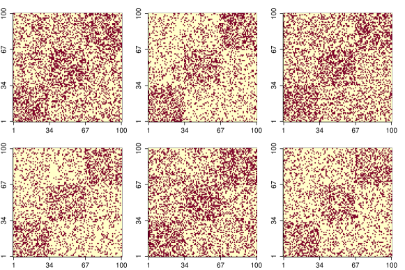
Figure 2: Examples of adjacency matrices generated from SBM with $\rho=0.5$ and $n=100$. In the first row, from left to right, each plot corresponds to the network at $t=25,50,75$ respectively. In the second row, from left to right, each plot corresponds to the network at $t=26,51,76$ respectively (the change points). In each display, a red dot indicates one and zero otherwise.

Figure 2 exhibits examples of generated networks at particular time points. Visually, Scenario 1 produces adjacency matrices with block structures, and mutuality is an important pattern in these networks. To detect the change points with our method, we use two network statistics, edge count and mutuality, in both formation and dissolution models. In the competitor methods, besides the dynamic networks $\{\bm{y}^{t}\}_{t=1}^{T}$, we also use the edge count and mutuality in $\{\bm{g}(\bm{y}^{t})\}_{t=1}^{T}$ as another specification. Tables 1, 2, and 3 display the means of evaluation metrics for different specifications.

Table 1: Means of evaluation metrics for dynamic networks simulated from the Stochastic Block Model with $\rho=0.0$.

$\rho$	$n$	Method	$|\hat{K}-K|$	$d(\hat{\mathcal{C}}|\mathcal{C})$	$d(\mathcal{C}|\hat{\mathcal{C}})$	$C(\mathcal{G},\mathcal{G^{\prime}})$
$0.0$	$50$	CPDstergm	$0.3$	$0.8$	$2.2$	$95.35\%$
		gSeg (nets.)	$2.9$	inf	$-\text{inf}$	$4.55\%$
		kerSeg (nets.)	$\bm{0}$	$\bm{0}$	$\bm{0}$	$\bm{100\%}$
		gSeg (stats.)	$2.1$	inf	$-\text{inf}$	$43.68\%$
		kerSeg (stats.)	$0.1$	$\bm{0}$	$0.3$	$99.70\%$
$0.0$	$100$	CPDstergm	$1$	$0.8$	$5.8$	$89.07\%$
		gSeg (nets.)	$2.9$	inf	$-\text{inf}$	$4.79\%$
		kerSeg (nets.)	$\bm{0}$	$\bm{0}$	$\bm{0}$	$\bm{100\%}$
		gSeg (stats.)	$1.9$	inf	$-\text{inf}$	$44.38\%$
		kerSeg (stats.)	$\bm{0}$	$\bm{0}$	$\bm{0}$	$\bm{100\%}$
$0.0$	$500$	CPDstergm	$\bm{0}$	$1$	$1$	$97.07\%$
		gSeg (nets.)	$3$	inf	$-\text{inf}$	$0\%$
		kerSeg (nets.)	$\bm{0}$	$\bm{0}$	$\bm{0}$	$\bm{100\%}$
		gSeg (stats.)	$2.1$	inf	$-\text{inf}$	$40.12\%$
		kerSeg (stats.)	$\bm{0}$	$\bm{0}$	$\bm{0}$	$\bm{100\%}$

Table 2: Means of evaluation metrics for dynamic networks simulated from the Stochastic Block Model with $\rho=0.5$.

$\rho$	$n$	Method	$|\hat{K}-K|$	$d(\hat{\mathcal{C}}|\mathcal{C})$	$d(\mathcal{C}|\hat{\mathcal{C}})$	$C(\mathcal{G},\mathcal{G^{\prime}})$
$0.5$	$50$	CPDstergm	$\bm{0.1}$	$1$	$\bm{2.4}$	$\bm{97.04\%}$
		gSeg (nets.)	$12.9$	$\bm{0}$	$19.4$	$27.20\%$
		kerSeg (nets.)	$6.4$	$\bm{0}$	$16.6$	$45.50\%$
		gSeg (stats.)	$1.8$	$36.6$	$5.8$	$56.04\%$
		kerSeg (stats.)	$0.7$	$\bm{0}$	$4.4$	$94.60\%$
$0.5$	$100$	CPDstergm	$\bm{0}$	$1$	$\bm{1}$	$\bm{98.04\%}$
		gSeg (nets.)	$12.3$	$\bm{0}$	$19$	$27.80\%$
		kerSeg (nets.)	$6$	$\bm{0}$	$15.2$	$47.00\%$
		gSeg (stats.)	$1.6$	inf	$-\text{inf}$	$53.50\%$
		kerSeg (stats.)	$0.9$	$\bm{0}$	$10$	$92.70\%$
$0.5$	$500$	CPDstergm	$\bm{0}$	$1$	$\bm{1}$	$\bm{98.04\%}$
		gSeg (nets.)	$12.3$	$\bm{0}$	$19.2$	$27.80\%$
		kerSeg (nets.)	$4$	$\bm{0}$	$12.7$	$52.20\%$
		gSeg (stats.)	$1.7$	$36.6$	$3.9$	$58.59\%$
		kerSeg (stats.)	$1.3$	$\bm{0}$	$7.4$	$91.40\%$

Table 3: Means of evaluation metrics for dynamic networks simulated from the Stochastic Block Model with $\rho=0.9$.

$\rho$	$n$	Method	$|\hat{K}-K|$	$d(\hat{\mathcal{C}}|\mathcal{C})$	$d(\mathcal{C}|\hat{\mathcal{C}})$	$C(\mathcal{G},\mathcal{G^{\prime}})$
$0.9$	$50$	CPDstergm	$\bm{0}$	$1$	$\bm{1}$	$\bm{98.04\%}$
		gSeg (nets.)	$12.6$	$\bm{0}$	$19.2$	$27.50\%$
		kerSeg (nets.)	$11$	$\bm{0}$	$18.7$	$32.00\%$
		gSeg (stats.)	$6.7$	$5.4$	$16.9$	$58.45\%$
		kerSeg (stats.)	$4.4$	$\bm{0}$	$14$	$70.80\%$
$0.9$	$100$	CPDstergm	$\bm{0}$	$1$	$\bm{1}$	$\bm{98.04\%}$
		gSeg (nets.)	$12.6$	$\bm{0}$	$19$	$27.50\%$
		kerSeg (nets.)	$12$	$\bm{0}$	$19$	$28.00\%$
		gSeg (stats.)	$5.6$	$1.6$	$18.8$	$62.66\%$
		kerSeg (stats.)	$4$	$\bm{0}$	$17.3$	$71.50\%$
$0.9$	$500$	CPDstergm	$\bm{0}$	$1$	$\bm{1}$	$\bm{98.04\%}$
		gSeg (nets.)	$12.2$	$\bm{0}$	$19$	$27.80\%$
		kerSeg (nets.)	$12$	$\bm{0}$	$19$	$28.00\%$
		gSeg (stats.)	$7.4$	$0.2$	$19.1$	$58.96\%$
		kerSeg (stats.)	$5.2$	$\bm{0}$	$19$	$66.90\%$

As expected, the kerSeg method can achieve a good performance on the covering metric $C(\mathcal{G},\mathcal{G^{\prime}})$ when $\rho=0$, since the time-independent setting aligns with the kerSeg’s assumption. However, the performances of gSeg and kerSeg are worsened when $\rho>0$. In particular, when the networks in the sequence are time-dependent, both gSeg and kerSeg methods can effectively detect the true change points, as the one-sided Hausdorff distance $d(\hat{\mathcal{C}}|\mathcal{C})$ are close to zeros. Yet the reversed one-sided Hausdorff distance $d(\mathcal{C}|\hat{\mathcal{C}})$ and the absolute error $|\hat{K}-K|$ show that both gSeg and kerSeg tend to detect excessive number of change points as the sequences of networks become noisier under the time-dependent condition. Our CPDstergm method, on average, achieves smaller absolute error, smaller one-sided Hausdorff distances, and greater coverage of interval partitions, regardless of the temporal dependence.

Another aspect worth mentioning is the usage of the network statistics in the competitor methods. The performance of gSeg and kerSeg, in terms of the covering metric $C(\mathcal{G},\mathcal{G^{\prime}})$, improves significantly when we change the input data from networks to network statistics, which demonstrates the potential of using network level summary statistics to represent the enormous amount of individual relations.

Scenario 2: Separable Temporal ERGM

In this scenario, we employ time-homogeneous STERGMs (Krivitsky and Handcock, 2014) between change points to generate sequences of dynamic networks, using the R package tergm (Krivitsky and Handcock, 2022). For the following three specifications, we gradually increase the complexity of the network patterns, by adding more network statistics in the data generating process. First we use two network statistics, edge count and mutuality, in both formation and dissolution models to let $p_{\text{sim}}=4$. The parameters are

$$\bm{\theta}^{+,t},\bm{\theta}^{-,t}=\begin{cases}-1,\ -2,\ -1,\ -2,&t\in\mathcal{A}_{1}\cup\mathcal{A}_{3},\\ -1,\ 1,\ -1,\ -1,&t\in\mathcal{A}_{2}\cup\mathcal{A}_{4}.\\ \end{cases}$$

Next, we include the number of triangles in both formation and dissolution models to let $p_{\text{sim}}=6$. The parameters are

$$\bm{\theta}^{+,t},\bm{\theta}^{-,t}=\begin{cases}-2,\ 2,\ -2,\ -1,\ 2,\ 1,&t\in\mathcal{A}_{1}\cup\mathcal{A}_{3},\\ -1.5,\ 1,\ -1,\ 2,\ 1,\ 1.5,&t\in\mathcal{A}_{2}\cup\mathcal{A}_{4}.\\ \end{cases}$$

Finally, we include the homophily for gender, an attribute assigned to each node, in both formation and dissolution models to let $p_{\text{sim}}=8$. The parameters are

$$\bm{\theta}^{+,t},\bm{\theta}^{-,t}=\begin{cases}-2,\ 2,\ -2,\ -1,\ -1,\ 2,\ 1,\ 1,&t\in\mathcal{A}_{1}\cup\mathcal{A}_{3},\\ -1.5,\ 1,\ -1,\ 1,\ 2,\ 1,\ 1.5,\ 2,&t\in\mathcal{A}_{2}\cup\mathcal{A}_{4}.\\ \end{cases}$$

The nodal attributes, $\bm{x}_{i}\in\{\text{Female},\text{Male}\}$ for $i\in[n]$, are fixed across time $t$ in the generation process.

Figure 3 exhibits examples of generated networks at particular time points. Specifically, Scenario 2 produces adjacency matrices that are sparse, which is often the case in reality. For comparison, to detect the change points with our method, we use the network statistics that generate the networks in both formation and dissolution models. In the competitor methods, besides the dynamic networks, we also use the same network statistics that generate the networks as another specification. Tables 4, 5, and 6 display the means of evaluation metrics for different specifications.

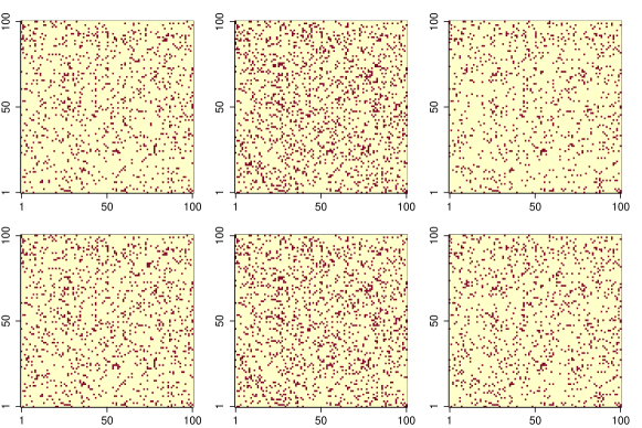
Figure 3: Examples of adjacency matrices generated from STERGM with $p_{\text{sim}}=6$ and $n=100$. In the first row, from left to right, each plot corresponds to the network at $t=25,50,75$ respectively. In the second row, from left to right, each plot corresponds to the network at $t=26,51,76$ respectively (the change points). In each display, a red dot indicates one and zero otherwise.

Table 4: Means of evaluation metrics for dynamic networks simulated from the STERGM with $p_{\text{sim}}=4$.

$p_{\text{sim}}$	$n$	Method	$|\hat{K}-K|$	$d(\hat{\mathcal{C}}|\mathcal{C})$	$d(\mathcal{C}|\hat{\mathcal{C}})$	$C(\mathcal{G},\mathcal{G^{\prime}})$
$4$	$50$	CPDstergm	$\bm{0}$	$0.1$	$0.1$	$99.80\%$
		gSeg (nets.)	$1.9$	$21.7$	$12$	$48.83\%$
		kerSeg (nets.)	$2.8$	$\bm{0}$	$15.8$	$78.30\%$
		gSeg (stats.)	$2.1$	inf	$-\text{inf}$	$43.61\%$
		kerSeg (stats.)	$\bm{0}$	$\bm{0}$	$\bm{0}$	$\bm{100\%}$
$4$	$100$	CPDstergm	$\bm{0}$	$\bm{0}$	$\bm{0}$	$\bm{100\%}$
		gSeg (nets.)	$1.8$	$18.2$	$17.1$	$44.20\%$
		kerSeg (nets.)	$2.6$	$\bm{0}$	$15.6$	$77.40\%$
		gSeg (stats.)	$2.1$	inf	$-\text{inf}$	$30.37\%$
		kerSeg (stats.)	$0.1$	$\bm{0}$	$0.2$	$99.80\%$
$4$	$500$	CPDstergm	$\bm{0}$	$1$	$\bm{1}$	$\bm{94.96\%}$
		gSeg (nets.)	$12$	$\bm{0}$	$19$	$28.00\%$
		kerSeg (nets.)	$4.6$	$1.7$	$14.4$	$51.65\%$
		gSeg (stats.)	$1.9$	$24.9$	$19.8$	$48.41\%$
		kerSeg (stats.)	$4.3$	$1.4$	$19.4$	$74.02\%$

For $p_{\text{sim}}=4$, the performance of the kerSeg method in terms of the covering metric $C(\mathcal{G},\mathcal{G^{\prime}})$ improves significantly when we change the input data from networks to network statistics. However, for $p_{\text{sim}}=6$, both gSeg and kerSeg methods tend to detect excessive number of change points when the networks are highly dyadic dependent due to the inclusion of the triangle term. Using network statistics as input can no longer improve their performance. Our CPDstergm method, which dissects the network evolution using formation and dissolution models, can achieve a good result when the networks are both temporal and dyadic dependent. Lastly, for $p_{\text{sim}}=8$, our method permits the inclusion of nodal attributes to facilitate the change detection, besides edge information. On average, our method produces smaller absolute error, smaller one-sided Hausdorff distances, and greater coverage of interval partitions.

Table 5: Means of evaluation metrics for dynamic networks simulated from the STERGM with $p_{\text{sim}}=6$.

$p_{\text{sim}}$	$n$	Method	$|\hat{K}-K|$	$d(\hat{\mathcal{C}}|\mathcal{C})$	$d(\mathcal{C}|\hat{\mathcal{C}})$	$C(\mathcal{G},\mathcal{G^{\prime}})$
$6$	$50$	CPDstergm	$\bm{0.2}$	$1.6$	$\bm{3}$	$\bm{91.54\%}$
		gSeg (nets.)	$12.3$	$\bm{0}$	$19$	$27.90\%$
		kerSeg (nets.)	$9.7$	$1.4$	$17.9$	$37.62\%$
		gSeg (stats.)	$15.8$	$1.5$	$20.1$	$24.55\%$
		kerSeg (stats.)	$9.4$	$3.9$	$18$	$35.86\%$
$6$	$100$	CPDstergm	$\bm{0}$	$1$	$\bm{1}$	$\bm{94.19\%}$
		gSeg (nets.)	$12$	$\bm{0}$	$19$	$28.00\%$
		kerSeg (nets.)	$9.6$	$1$	$17.5$	$37.66\%$
		gSeg (stats.)	$14.9$	$1.9$	$20.3$	$26.13\%$
		kerSeg (stats.)	$8$	$5.4$	$16.7$	$38.45\%$
$6$	$500$	CPDstergm	$\bm{0}$	$1$	$\bm{1}$	$\bm{98.04\%}$
		gSeg (nets.)	$12$	$\bm{0}$	$19$	$28.00\%$
		kerSeg (nets.)	$8.3$	$0.2$	$16.4$	$42.20\%$
		gSeg (stats.)	$1.7$	$45.1$	$4.6$	$49.27\%$
		kerSeg (stats.)	$6.1$	$3.1$	$15.3$	$55.24\%$

Table 6: Means of evaluation metrics for dynamic networks simulated from the STERGM with $p_{\text{sim}}=8$.

$p_{\text{sim}}$	$n$	Method	$|\hat{K}-K|$	$d(\hat{\mathcal{C}}|\mathcal{C})$	$d(\mathcal{C}|\hat{\mathcal{C}})$	$C(\mathcal{G},\mathcal{G^{\prime}})$
$8$	$50$	CPDstergm	$\bm{0.4}$	$1.7$	$\bm{4.4}$	$\bm{89.56\%}$
		gSeg (nets.)	$13.3$	$\bm{0}$	$19.6$	$27.20\%$
		kerSeg (nets.)	$9.5$	$0.8$	$18.2$	$37.86\%$
		gSeg (stats.)	$13.4$	$2.3$	$19.7$	$28.00\%$
		kerSeg (stats.)	$8.7$	$4.8$	$18.3$	$36.51\%$
$8$	$100$	CPDstergm	$\bm{0}$	$1.6$	$\bm{1.6}$	$\bm{93.11\%}$
		gSeg (nets.)	$12$	$\bm{0}$	$19$	$28.00\%$
		kerSeg (nets.)	$9.3$	$1.7$	$17.6$	$37.12\%$
		gSeg (stats.)	$12.8$	$4.2$	$19.5$	$28.08\%$
		kerSeg (stats.)	$8.2$	$5.8$	$18.6$	$36.55\%$
$8$	$500$	CPDstergm	$\bm{0.4}$	$12.3$	$\bm{2.3}$	$\bm{85.71\%}$
		gSeg (nets.)	$12$	$\bm{0}$	$19$	$28.00\%$
		kerSeg (nets.)	$8.9$	$2$	$14.5$	$43.00\%$
		gSeg (stats.)	$5.1$	$20.2$	$20.7$	$32.08\%$
		kerSeg (stats.)	$9.6$	$2$	$17$	$37.95\%$

5.2 MIT Cellphone Data

The Massachusetts Institute of Technology (MIT) cellphone data (Eagle and Pentland, 2006) consists of human interactions via cellphone activity, among $n=96$ participants for a duration of $T=232$ days. The data were taken from 2004-09-15 to 2005-05-04 inclusive, which covers the winter and spring vacations in the MIT 2004-2005 academic calendar. For participant $i$ and participant $j$, a connected edge $\bm{y}_{ij}^{t}=1$ indicates that they had made at least one phone call on day $t$, and $\bm{y}_{ij}^{t}=0$ indicates that they had made no phone call on day $t$.

As the data portrays human interactions, we use the number of (1) edges, (2) isolates, and (3) triangles to represent the occurrence of connections, the sparsity of social networks, and the transitive association of friendship, respectively. The three network statistics are used in both formation and dissolution models of our method. For the competitors, we use the three network statistics $\bm{g}(\bm{y}^{t})$ as input data, since they provide better results than using the networks $\bm{y}^{t}$. Figure 4 displays $\Delta\hat{\bm{\zeta}}$ of Equation (14) and the detected change points of our method, as well as the results from the competitors. Moreover, Table 7 provides a list of potential nearby events that align with the detected change points of our method.

The two shaded areas in Figure 4 correspond to the winter and spring vacations, and our method can punctually detect the pattern change in the contact behaviors. Both gSeg and kerSeg can also detect the beginning of the winter vacation, but their results on the spring vacation are slightly deviated. Furthermore, we detect a few spikes in the middle of October 2004, which correspond to the annual sponsor meeting that happened on 2004-10-21. About two-thirds of the participants have prepared and attended the annual sponsor meeting, and the majority of their time has contributed to achieve project goals throughout the week (Eagle and Pentland, 2006).

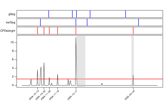
Figure 4: Visualization of $\Delta\hat{\bm{\zeta}}$ and the detected change points from our method for the MIT cellphone data. The detected change points from the competitors are also displayed. The two shaded areas correspond to the winter and spring vacations in the MIT 2004-2005 academic calendar. The data-driven threshold (red horizontal line) is calculated by (15) with $\mathcal{Z}_{0.9}$.

Table 7: Potential nearby events that align with the detected change points (CP) of our method

Detected CP	Potential nearby events
2004-10-13	Preparation for the Sponsor meeting
2004-10-24	2004-10-21 (Sponsor meeting)
2004-11-02	2004-11-02 (Presidential election)
2004-11-16	2004-11-17 (Last day to cancel subjects)
2004-12-17	2004-12-18 to 2005-01-02 (Winter vacation)
2005-03-24	2005-03-21 to 2005-03-25 (Spring vacation)

5.3 Stock Market Data

The stock market data consists of the weekly log returns of $29$ stocks included in the Dow Jones Industrial Average (DJIA) index, and it is available in the R package ecp (James and Matteson, 2015). We consider the data from 2007-01-01 to 2010-01-04, which covers the 2008 worldwide economic crisis. We focus on the negative correlations among stock returns to detect the systematic anomalies in the financial market. Specifically, we first use a sliding window of width $4$ to calculate the correlation matrices of the weekly log returns. We then truncate the correlation matrices by setting those entries which have negative values as $1$, and the remaining as $0$.

In the $T=158$ networks, a connected edge $\bm{y}_{ij}^{t}=1$ indicates the log returns of stock $i$ and stock $j$ are negative correlated over the four-week period that ends at week $t$. Moreover, the number of triangles can signify the volatility of the stock market, as the three stocks are mutually negative correlated. In general, the more triangles in a network, the more opposite movements among the stock returns, suggesting a large fluctuation in the market. On the contrary, when the number of triangles is small, the majority of the stock returns either increase or decrease at the same time, suggesting a stable trend in the market. To this end, we use the number of edges and triangles in both formation and dissolution models of our method. For the competitors, we use the networks $\bm{y}^{t}$ as input data, since they provide better results than using the networks statistics $\bm{g}(\bm{y}^{t})$. Figure 5 displays $\Delta\hat{\bm{\zeta}}$ of Equation (14) and the detected change points of our method, as well as the results from the competitors.

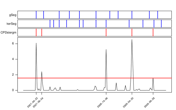
Figure 5: Visualization of $\Delta\hat{\bm{\zeta}}$ and the detected change points from our method for the stock market data. The detected change points from the competitors are also displayed. The data-driven threshold (red horizontal line) is calculated by (15) with $\mathcal{Z}_{0.9}$.

As expected, the stock market is volatile. The competitors have detected excessive number of change points, aligning with the smaller spikes in $\Delta\hat{\bm{\zeta}}$. Those change points can be detected by our method, if we manually lower the threshold to adjust the sensitivity. In this experiment, we focus on the top three spikes for real event interpretation. Table 8 presents the three detected change points and the potential nearby events. Given the networks are constructed using a sliding window, a detected change point indicates the pattern changes occur amid the four-week time span. As supporting evidence, the New Century Financial Corporation (NCFC) was the largest U.S. subprime mortgage lender in 2007, and the Lehman Brothers (LB) was one of the largest investment banks. Their bankruptcies caused by the collapse of the mortgage industry severely fueled the worldwide financial crisis, which also led the DJIA to the bottom.

Table 8: Potential nearby events that align with the top three detected change points (CP) of our method

Detected CP	Potential nearby events
2007-04-23	2007-04-02 (NCFC filed for bankruptcy)
2008-10-06	2008-09-15 (LB filed for bankruptcy)
2009-04-20	2009-03-09 (DJIA bottomed)

6 Discussion

In this work, we study the change point detection problem in time series of graphs, which can serve as a prerequisite for dynamic network analysis. Essentially, we fit a time-heterogeneous STERGM while penalizing the sum of Euclidean norms of the parameter differences between consecutive time steps. The objective function with the Group Fused Lasso penalty is solved via Alternating Direction Method of Multipliers, and we adopt the pseudo-likelihood of STERGM to expedite the parameter estimation.

The STERGM (Krivitsky and Handcock, 2014) used in our method is a flexible model to fit dynamic networks with both dyadic and temporal dependence. It manages dyad formation and dissolution separately, as the underlying reasons that induce the two processes are usually different in reality. Furthermore, the ERGM suite (Handcock et al., 2022) provides an extensive list of network statistics to capture the structural changes, and we develop an R package CPDstergm to implement the proposed method.

Several improvements to our change point detection method are possible. Relational phenomena by nature have degrees of strength, and dichotomizing valued networks into binary networks may introduce biases for analysis (Thomas and Blitzstein, 2011). We can extend the STERGM with a valued ERGM (Krivitsky, 2012; Desmarais and Cranmer, 2012a; Caimo and Gollini, 2020) to facilitate change point detection in dynamic valued networks. Moreover, the number of participants and their attributes are subject to change over time. It is necessary for a change point detection method to adjust the network sizes as in Krivitsky et al. (2011), and to adapt the time-evolving nodal attributes by incorporating the Exponential-family Random Network Model (ERNM) as in Fellows and Handcock (2012) and Fellows and Handcock (2013).

Newton-Raphson Method for Updating $\bm{\theta}$

In this appendix, we derive the gradient and Hessian for the Newton-Raphson method to update $\bm{\theta}$. The first-order derivative of $l(\bm{\theta})$ with respect to $\bm{\theta}^{+,t}$, the parameter in the formation model at a particular time point $t$, is

$$\begin{split}\nabla_{\bm{\theta}^{+,t}}\ l(\bm{\theta})&=\sum_{ij}\Big{\{}\bm{y}_{ij}^{+,t}\Delta g_{ij}^{+}(\bm{y}^{+,t})-\frac{\exp[\bm{\theta}^{+,t}\cdot\Delta g_{ij}^{+}(\bm{y}^{+,t})]}{1+\exp[\bm{\theta}^{+,t}\cdot\Delta g_{ij}^{+}(\bm{y}^{+,t})]}\Delta g_{ij}^{+}(\bm{y}^{+,t})\Big{\}}\end{split}$$

$$=\sum_{ij}(\bm{y}_{ij}^{+,t}-\bm{\mu}_{ij}^{+,t})[\Delta g_{ij}^{+}(\bm{y}^{+,t})]$$

where $\bm{\mu}_{ij}^{+,t}=h(\bm{\theta}^{+,t}\cdot\Delta\bm{g}_{ij}^{+}(\bm{y}^{+,t}))$. The $h(x)=1/(1+\exp(-x))$ is the element-wise sigmoid function. Likewise, the first-order derivative of $l(\bm{\theta})$ with respect to $\bm{\theta}^{-,t}$, the parameter in the dissolution model at a particular time point $t$, is similar except for notational difference.

Denote the objective function in (8) as $\mathcal{L}_{\alpha}(\bm{\theta})$. To update the parameters $\bm{\theta}\in\mathbb{R}^{\tau\times p}$ in a compact form, we first vectorize it as $\vv{\bm{\theta}}=\text{vec}_{\tau p}(\bm{\theta})\in\mathbb{R}^{\tau p\times 1}$. The matrices $\bm{z}\in\mathbb{R}^{\tau\times p}$ and $\bm{u}\in\mathbb{R}^{\tau\times p}$ are also vectorized as $\vv{\bm{z}}=\text{vec}_{\tau p}(\bm{z})\in\mathbb{R}^{\tau p\times 1}$ and $\vv{\bm{u}}=\text{vec}_{\tau p}(\bm{u})\in\mathbb{R}^{\tau p\times 1}$. With the constructed matrices $\bm{H}\in\mathbb{R}^{2\tau E\times\tau p}$ and $\bm{W}\in\mathbb{R}^{2\tau E\times 2\tau E}$, the gradient of $\mathcal{L}_{\alpha}(\bm{\theta})$ with respect to $\vv{\bm{\theta}}$ is

$$\nabla_{\vv{\bm{\theta}}}\ \mathcal{L}_{\alpha}(\bm{\theta})=-\bm{H}^{\top}(\vv{\bm{y}}-\vv{\bm{\mu}})+\alpha\big{(}\vv{\bm{\theta}}-\vv{\bm{z}}^{(a)}+\vv{\bm{u}}^{(a)}\big{)}$$

where $\vv{\bm{\mu}}=h(\bm{H}\cdot\vv{\bm{\theta}})\in\mathbb{R}^{2\tau E\times 1}$.

Furthermore, the second order derivative of $l(\bm{\theta})$ with respect to $\bm{\theta}^{+,t}$ is

$\begin{aligned} \nabla_{\bm{\theta}^{+,t}}^{2}\ l(\bm{\theta})&=\sum_{ij}-\bm{\mu}_{ij}^{+,t}(1-\bm{\mu}_{ij}^{+,t})[\Delta\bm{g}_{ij}^{+}(\bm{y}^{+,t})\Delta\bm{g}_{ij}^{+}(\bm{y}^{+,t})^{\top}]\end{aligned}$

and the second order derivative of $l(\bm{\theta})$ with respect to $\bm{\theta}^{-,t}$ is similar except for notational difference. Thus, the Hessian of $\mathcal{L}_{\alpha}(\bm{\theta})$ with respect to $\vv{\bm{\theta}}\in\mathbb{R}^{\tau p\times 1}$ is

$$\nabla_{\vv{\bm{\theta}}}^{2}\ \mathcal{L}_{\alpha}(\bm{\theta})=\bm{H}^{\top}\bm{W}\bm{H}+\alpha\bm{I}_{\tau p}$$

where $\bm{I}_{\tau p}$ is the identity matrix. For fast implementation, it is possible to use the diagonal Hessian to approximate the above Hessian matrix. By using the Newton-Raphson method, the $\vv{\bm{\theta}}\in\mathbb{R}^{\tau p\times 1}$ is updated as

$$\vv{\bm{\theta}}_{c+1}= \vv{\bm{\theta}}_{c}-\big{(}\bm{H}^{\top}\bm{W}\bm{H}+\alpha\bm{I}_{\tau p}\big{)}^{-1}\cdot\big{(}-\bm{H}^{\top}(\vv{\bm{y}}-\vv{\bm{\mu}})+\alpha(\vv{\bm{\theta}}_{c}-\vv{\bm{z}}^{(a)}+\vv{\bm{u}}^{(a)})\big{)}$$

where $c$ denotes the current Newton-Raphson iteration. Note that both $\bm{W}$ and $\vv{\bm{\mu}}$ are also calculated based on $\vv{\bm{\theta}}_{c}$.

Group Lasso for Updating $\bm{\beta}$

In this appendix, we present the derivation of learning $\bm{\beta}$, which is equivalent to solving a Group Lasso problem. Denote the objective function in (9) as $\mathcal{L}_{\alpha}(\bm{\gamma},\bm{\beta})$. When $\bm{\beta}_{i,\bm{\cdot}}\neq\bm{0}$, the first-order derivative of $\mathcal{L}_{\alpha}(\bm{\gamma},\bm{\beta})$ with respect to $\bm{\beta}_{i,\bm{\cdot}}$ is

$$\frac{\partial}{\partial\bm{\beta}_{i,\bm{\cdot}}} \mathcal{L}_{\alpha}(\bm{\gamma},\bm{\beta})=\lambda\frac{\bm{\beta}_{i,\bm{\cdot}}}{\lVert\bm{\beta}_{i,\bm{\cdot}}\rVert_{2}}-\alpha\bm{X}_{\bm{\cdot},i}^{\top}(\bm{\theta}^{(a+1)}+\bm{u}^{(a)}-\bm{1}_{\tau,1}\bm{\gamma}-\bm{X}_{\bm{\cdot},i}\bm{\beta}_{i,\bm{\cdot}}-\bm{X}_{\bm{\cdot},-i}\bm{\beta}_{-i,\bm{\cdot}})$$

where $\bm{X}_{\bm{\cdot},i}\in\mathbb{R}^{\tau\times 1}$ is the $i$th column of matrix $\bm{X}\in\mathbb{R}^{\tau\times(\tau-1)}$ and $\bm{\beta}_{i,\bm{\cdot}}\in\mathbb{R}^{1\times p}$ is the $i$th row of matrix $\bm{\beta}\in\mathbb{R}^{(\tau-1)\times p}$. Setting the gradient to $\bm{0}$, we have

$$\bm{\beta}_{i,\bm{\cdot}}=(\alpha\bm{X}_{\bm{\cdot},i}^{\top}\bm{X}_{\bm{\cdot},i}+\frac{\lambda}{\lVert\bm{\beta}_{i,\bm{\cdot}}\rVert}_{2})^{-1}\bm{s}_{i}$$ (17)

where

$$\bm{s}_{i}=\alpha\bm{X}_{\bm{\cdot},i}^{\top}(\bm{\theta}^{(a+1)}+\bm{u}^{(a)}-\bm{1}_{\tau,1}\bm{\gamma}-\bm{X}_{\bm{\cdot},-i}\bm{\beta}_{-i,\bm{\cdot}}).$$

Taking the Euclidean norm of (17) on both sides and rearrange the terms, we have

$$\lVert\bm{\beta}_{i,\bm{\cdot}}\rVert_{2}=(\alpha\bm{X}_{\bm{\cdot},i}^{\top}\bm{X}_{\bm{\cdot},i})^{-1}(\lVert\bm{s}_{i}\rVert_{2}-\lambda).$$

Plugging $\lVert\bm{\beta}_{i,\bm{\cdot}}\rVert_{2}$ into (17), the solution of $\bm{\beta}_{i,\bm{\cdot}}$ is

$$\bm{\beta}_{i,\bm{\cdot}}=\frac{1}{\alpha\bm{X}_{\bm{\cdot},i}^{\top}\bm{X}_{\bm{\cdot},i}}(1-\frac{\lambda}{\lVert\bm{s}_{i}\rVert_{2}})\bm{s}_{i}.$$

When $\bm{\beta}_{i,\bm{\cdot}}=\bm{0}$, the subgradient $\bm{v}$ of $\lVert\bm{\beta}_{i,\bm{\cdot}}\rVert_{2}$ needs to satisfy $\lVert\bm{v}\rVert_{2}\leq 1$. Since

$$\bm{0}\in\lambda\bm{v}-\alpha\bm{X}_{\bm{\cdot},i}^{\top}(\bm{\theta}^{(a+1)}+\bm{u}^{(a)}-\bm{1}_{\tau,1}\bm{\gamma}-\bm{X}_{\bm{\cdot},-i}\bm{\beta}_{-i,\bm{\cdot}}),$$

we obtain the condition that $\bm{\beta}_{i,\bm{\cdot}}$ becomes $\bm{0}$ if $\lVert\bm{s}_{i}\rVert_{2}\leq\lambda$. Therefore, we can iteratively apply the following equation to update $\bm{\beta}_{i,\bm{\cdot}}$ for each $i=1,\dots,\tau-1$:

$$\bm{\beta}_{i,\bm{\cdot}}\leftarrow\frac{1}{\alpha\bm{X}_{\bm{\cdot},i}^{\top}\bm{X}_{\bm{\cdot},i}}\Big{(}1-\frac{\lambda}{\lVert\bm{s}_{i}\rVert_{2}}\Big{)}_{+}\bm{s}_{i}$$

where $(\cdot)_{+}=\max(\cdot,0)$. The matrix $\bm{X}\in\mathbb{R}^{\tau\times(\tau-1)}$ is constructed from the position dependent weight $\bm{d}\in\mathbb{R}^{\tau-1}$.

Network Statistics in Experiments

In this section, we provide the formulations of the network statistics used in the simulation and real data experiments. The network statistics of interest are chosen from the extensive list in ergm (Handcock et al., 2022), an R library for network analysis. Tables 9 and 10 display the formulations of network statistics used in the respective formation and dissolution models of our method for $t=2,\dots,T$. Moreover, Table 11 displays the formulations of network statistics used in the competitor methods for $t=1,\dots,T$. The formulations are referred to directed networks, and those for undirected networks are similar.

Table 9: Network statistics used in the formation model

Network Statistics	Formulation of $\bm{g}^{+}(\bm{y}^{+,t})$
Edge Count	$\sum_{ij}\bm{y}_{ij}^{+,t}$
Mutuality	$\sum_{i<j}\bm{y}_{ij}^{+,t}\bm{y}_{ji}^{+,t}$
Triangles	$\sum_{ijk}\bm{y}_{ij}^{+,t}\bm{y}_{jk}^{+,t}\bm{y}_{ik}^{+,t}+\sum_{ij<k}\bm{y}_{ij}^{+,t}\bm{y}_{jk}^{+,t}\bm{y}_{ki}^{+,t}$
Homophily	$\sum_{ij}\bm{y}_{ij}^{+,t}\times\mathbbm{1}(\bm{x}_{i}=\bm{x}_{j})$
Isolates	$\sum_{i}\mathbbm{1}\big{(}\text{deg}_{\text{in}}(\bm{y}^{+,t},i)=0\land\text{deg}_{\text{out}}(\bm{y}^{+,t},i)=0\big{)}$

Table 10: Network statistics used in the dissolution model

Network Statistics	Formulation of $\bm{g}^{-}(\bm{y}^{-,t})$
Edge Count	$\sum_{ij}\bm{y}_{ij}^{-,t}$
Mutuality	$\sum_{i<j}\bm{y}_{ij}^{-,t}\bm{y}_{ji}^{-,t}$
Triangles	$\sum_{ijk}\bm{y}_{ij}^{-,t}\bm{y}_{jk}^{-,t}\bm{y}_{ik}^{-,t}+\sum_{ij<k}\bm{y}_{ij}^{-,t}\bm{y}_{jk}^{-,t}\bm{y}_{ki}^{-,t}$
Homophily	$\sum_{ij}\bm{y}_{ij}^{-,t}\times\mathbbm{1}(\bm{x}_{i}=\bm{x}_{j})$
Isolates	$\sum_{i}\mathbbm{1}\big{(}\text{deg}_{\text{in}}(\bm{y}^{-,t},i)=0\land\text{deg}_{\text{out}}(\bm{y}^{-,t},i)=0\big{)}$

Table 11: Network statistics used in the competitor methods

Network Statistics	Formulation of $\bm{g}(\bm{y}^{t})$
Edge Count	$\sum_{ij}\bm{y}_{ij}^{t}$
Mutuality	$\sum_{i<j}\bm{y}_{ij}^{t}\bm{y}_{ji}^{t}$
Triangles	$\sum_{ijk}\bm{y}_{ij}^{t}\bm{y}_{jk}^{t}\bm{y}_{ik}^{t}+\sum_{ij<k}\bm{y}_{ij}^{t}\bm{y}_{jk}^{t}\bm{y}_{ki}^{t}$
Homophily	$\sum_{ij}\bm{y}_{ij}^{t}\times\mathbbm{1}(\bm{x}_{i}=\bm{x}_{j})$
Isolates	$\sum_{i}\mathbbm{1}\big{(}\text{deg}_{\text{in}}(\bm{y}^{t},i)=0\land\text{deg}_{\text{out}}(\bm{y}^{t},i)=0\big{)}$

References

- Alaíz et al. (2013) Carlos M Alaíz, Alvaro Barbero, and José R Dorronsoro. Group fused lasso. In Artificial Neural Networks and Machine Learning–ICANN 2013: 23rd International Conference on Artificial Neural Networks Sofia, Bulgaria, September 10-13, 2013. Proceedings 23, pages 66–73. Springer, 2013.
- Besag (1974) Julian Besag. Spatial interaction and the statistical analysis of lattice systems. Journal of the Royal Statistical Society: Series B (Methodological), 36(2):192–225, 1974.
- Blackburn and Handcock (2022) Bart Blackburn and Mark S Handcock. Practical network modeling via tapered exponential-family random graph models. Journal of Computational and Graphical Statistics, pages 1–14, 2022.
- Bleakley and Vert (2011) Kevin Bleakley and Jean-Philippe Vert. The group fused lasso for multiple change-point detection. arXiv preprint arXiv:1106.4199, 2011.
- Boyd et al. (2011) Stephen Boyd, Neal Parikh, Eric Chu, Borja Peleato, Jonathan Eckstein, et al. Distributed optimization and statistical learning via the alternating direction method of multipliers. Foundations and Trends® in Machine Learning, 3(1):1–122, 2011.
- Bybee and Atchadé (2018) Leland Bybee and Yves Atchadé. Change-point computation for large graphical models: A scalable algorithm for gaussian graphical models with change-points. Journal of Machine Learning Research, 19(11):1–38, 2018.
- Caimo and Friel (2011) Alberto Caimo and Nial Friel. Bayesian inference for exponential random graph models. Social networks, 33(1):41–55, 2011.
- Caimo and Gollini (2020) Alberto Caimo and Isabella Gollini. A multilayer exponential random graph modelling approach for weighted networks. Computational Statistics & Data Analysis, 142:106825, 2020.
- Chen et al. (2020a) Guodong Chen, Jesús Arroyo, Avanti Athreya, Joshua Cape, Joshua T Vogelstein, Youngser Park, Chris White, Jonathan Larson, Weiwei Yang, and Carey E Priebe. Multiple network embedding for anomaly detection in time series of graphs. arXiv preprint arXiv:2008.10055, 2020a.
- Chen (2019) Hao Chen. Sequential change-point detection based on nearest neighbors. The Annals of Statistics, 47(3):1381–1407, 2019.
- Chen and Zhang (2015) Hao Chen and Nancy Zhang. Graph-based change-point detection. The Annals of Statistics, 43(1):139–176, 2015.
- Chen et al. (2020b) Hao Chen, Nancy R. Zhang, Lynna Chu, and Hoseung Song. gSeg: Graph-Based Change-Point Detection (g-Segmentation), 2020b. URL https://CRAN.R-project.org/package=gSeg. R package version 1.0.
- Chu and Chen (2019) Lynna Chu and Hao Chen. Asymptotic distribution-free change-point detection for multivariate and non-euclidean data. The Annals of Statistics, 47(1):382–414, 2019.
- Desmarais and Cranmer (2012a) Bruce A Desmarais and Skyler J Cranmer. Statistical inference for valued-edge networks: The generalized exponential random graph model. PloS one, 7(1):e30136, 2012a.
- Desmarais and Cranmer (2012b) Bruce A Desmarais and Skyler J Cranmer. Statistical mechanics of networks: Estimation and uncertainty. Physica A: Statistical Mechanics and its Applications, 391(4):1865–1876, 2012b.
- Donnat and Holmes (2018) Claire Donnat and Susan Holmes. Tracking network dynamics: A survey using graph distances. The Annals of Applied Statistics, 12(2):971–1012, 2018.
- Eagle and Pentland (2006) Nathan Eagle and Alex (Sandy) Pentland. Reality mining: sensing complex social systems. Personal and Ubiquitous Computing, 10(4):255–268, 2006.
- Fellows and Handcock (2012) Ian Fellows and Mark S. Handcock. Exponential-family random network models. arXiv preprint arxiv:1208.0121, 2012.
- Fellows and Handcock (2013) Ian E Fellows and Mark S Handcock. Analysis of partially observed networks via exponential-family random network models. arXiv preprint arXiv:1303.1219, 2013.
- Fritz et al. (2021) Cornelius Fritz, Emilio Dorigatti, and David Rügamer. Combining graph neural networks and spatio-temporal disease models to predict covid-19 cases in germany. arXiv preprint arXiv:2101.00661, 2021.
- Geyer and Thompson (1992) Charles J Geyer and Elizabeth A Thompson. Constrained monte carlo maximum likelihood for dependent data. Journal of the Royal Statistical Society: Series B (Methodological), 54(3):657–683, 1992.
- Goyal and De Gruttola (2020) Ravi Goyal and Victor De Gruttola. Dynamic network prediction. Network Science, 8(4):574–595, 2020.
- Handcock et al. (2003) Mark S Handcock, Garry Robins, Tom Snijders, Jim Moody, and Julian Besag. Assessing degeneracy in statistical models of social networks. Technical report, Working paper, 2003.
- Handcock et al. (2007) Mark S Handcock, Adrian E Raftery, and Jeremy M Tantrum. Model-based clustering for social networks. Journal of the Royal Statistical Society: Series A (Statistics in Society), 170(2):301–354, 2007.
- Handcock et al. (2022) Mark S. Handcock, David R. Hunter, Carter T. Butts, Steven M. Goodreau, Pavel N. Krivitsky, and Martina Morris. ergm: Fit, Simulate and Diagnose Exponential-Family Models for Networks. The Statnet Project (https://statnet.org), 2022. URL https://CRAN.R-project.org/package=ergm. R package version 4.3.2.
- Hanneke et al. (2010) Steve Hanneke, Wenjie Fu, and Eric P Xing. Discrete temporal models of social networks. Electronic Journal of Statistics, 4:585–605, 2010.
- Hummel et al. (2012) Ruth M Hummel, David R Hunter, and Mark S Handcock. Improving simulation-based algorithms for fitting ergms. Journal of Computational and Graphical Statistics, 21(4):920–939, 2012.
- Hunter and Handcock (2006) David R Hunter and Mark S Handcock. Inference in curved exponential family models for networks. Journal of Computational and Graphical Statistics, 15(3):565–583, 2006.
- Hunter et al. (2008a) David R Hunter, Steven M Goodreau, and Mark S Handcock. Goodness of fit of social network models. Journal of the American Statistical Association, 103(481):248–258, 2008a.
- Hunter et al. (2008b) David R. Hunter, Mark S. Handcock, Carter T. Butts, Steven M. Goodreau, and Martina Morris. ergm: A package to fit, simulate and diagnose exponential-family models for networks. Journal of Statistical Software, 24(3):1–29, 2008b.
- James and Matteson (2015) Nicholas A. James and David S. Matteson. ecp: An r package for nonparametric multiple change point analysis of multivariate data. Journal of Statistical Software, 62(7):1–25, 2015. doi: 10.18637/jss.v062.i07. URL https://www.jstatsoft.org/index.php/jss/article/view/v062i07.
- Jiang et al. (2020) Binyan Jiang, Jailing Li, and Qiwei Yao. Autoregressive networks. arXiv preprint arXiv:2010.04492, 2020.
- Kei et al. (2023) Yik Lun Kei, Yanzhen Chen, and Oscar Hernan Madrid Padilla. A partially separable model for dynamic valued networks. Computational Statistics & Data Analysis, page 107811, 2023.
- Kolar et al. (2010) Mladen Kolar, Le Song, Amr Ahmed, and Eric P Xing. Estimating time-varying networks. The Annals of Applied Statistics, pages 94–123, 2010.
- Krivitsky (2012) Pavel N Krivitsky. Exponential-family random graph models for valued networks. Electronic Journal of Statistics, 6:1100, 2012.
- Krivitsky (2017) Pavel N Krivitsky. Using contrastive divergence to seed monte carlo mle for exponential-family random graph models. Computational Statistics & Data Analysis, 107:149–161, 2017.
- Krivitsky and Handcock (2014) Pavel N Krivitsky and Mark S Handcock. A separable model for dynamic networks. Journal of the Royal Statistical Society. Series B, Statistical Methodology, 76(1):29, 2014.
- Krivitsky and Handcock (2022) Pavel N. Krivitsky and Mark S. Handcock. tergm: Fit, Simulate and Diagnose Models for Network Evolution Based on Exponential-Family Random Graph Models. The Statnet Project (https://statnet.org), 2022. URL https://CRAN.R-project.org/package=tergm. R package version 4.1.0.
- Krivitsky et al. (2011) Pavel N Krivitsky, Mark S Handcock, and Martina Morris. Adjusting for network size and composition effects in exponential-family random graph models. Statistical Methodology, 8(4):319–339, 2011.
- Larroca et al. (2021) Federico Larroca, Paola Bermolen, Marcelo Fiori, and Gonzalo Mateos. Change point detection in weighted and directed random dot product graphs. In 2021 29th European Signal Processing Conference (EUSIPCO), pages 1810–1814. IEEE, 2021.