$d$-wave Charge-$4e$ Superconductivity From Fluctuating Pair Density Waves

Abstract

In this work we show that in several microscopic models for the pair-density-wave (PDW) state, when the PDW wave vectors connect special parts of the Fermi surface, the predominant instability driven by PDW fluctuations is toward a pairing state of the PDW boson themselves, realizing a long-saught-after charge-$4e$ superconductor. Dual to the scenario for electron pairing, the effective attraction between the bosons is mediated by exchanging low-energy fermions. In particular we show that the pairing interaction for the charge-$4e$ order is repulsive in the $s$-wave channel but attractive in the $d$-wave one. By analyzing the Ginzburg-Landau free energy including the fluctuation effects of PDW, within a large-$M$ extension of the theory, we find that the charge-$4e$ superconductivity emerges as a vestigial order of PDW, and sets in via a first-order transition.

I Introduction

Charge-$4e$ superconductivity ($4e$-SC) is an exotic order in which four fermions are bound together and condense [1, 2, 3, 4, 5]. Compared with the more common charge-$2e$ superconductivity ($2e$-SC), it breaks the global $U(1)$ symmetry to a discrete $\mathbb{Z}_{4}$ symmetry. Moreover, a vortex core in a $4e$-SC supports half flux quanta, which was recently claimed to have been observed in Kagome metal CsV₃Sb₅ [6]. On the theory side, recent progress have been made in understanding the properties of a mean-field $4e$-SC, which is in general an interacting system. It was found [7] that $4e$-SC is indeed a perfect conductor with nonzero superfluid density, but is in general a gapless system that shares many features with the Fermi liquid. However, the mechanism for $4e$-SC from interacting fermions remains a theoretical challenge. Unlike $2e$-SC which follows from an arbitrarily weak attractive interaction, there lacks a logarithmic divergence for the “quadrupling” (as opposed to pairing) susceptibility for $4e$-SC. Therefore, a theoretical understanding of $4e$-SC, even at the mean-field level, requires a non-perturbative description [7, 8].

In recent years, a promising framework for understanding $4e$-SC has emerged from the perspective of intertwined orders [9], in which a plethora of orders breaking distinct symmetries can naturally emerge from the partial melting of certain primary electronic orders. For instance, it has been suggested that from the fluctuations of a charge-$2e$ pair-density-wave (PDW) order [10, 11, 12, 13] or degenerate nematic charge-$2e$ superconducting order [14, 15], the $4e$-SC can appear as a vestigial order in the sense that it restores only partial broken symmetry of the primary orders. However, the starting point of such analyses is typically a Ginzburg-Landau theory for the primary orders, and when the underlying fermionic models are taken into full account, the intrinsic leading instability toward $4e$-SC are in general subleading to those toward non-superconducting states, either nematic or ferromagnetic [14, 16, 17]. It remains a major theoretical challenge to search for microscopic mechanisms for $4e$-SC as a leading instability.

In this work, we directly demonstrate that in a range of two-dimensional (2d) fermionic models with PDW instabilities, a $4e$-SC order naturally emerges as the leading instability once fluctuation effects are taken into account. Furthermore, we show that the resulting $4e$-SC order has a $d$-wave symmetry. As in previous works, the starting point of our theory, the PDW state, is by itself an exotic type of superconductivity with Cooper pairs carrying non-zero momenta [18, 19, 20, 21, 22, 23, 24, 25], which, despite being proposed to exist in many materials, most notably in the underdoped cuprates and in Kagome metals, in general requires unconventional mechanisms [26, 27, 28, 29, 30, 31, 32, 33, 34, 35, 36, 37, 35, 38, 39, 40, 41] to emerge. Encouragingly, it has been revealed recently [27] that PDW instabilities may be the leading pairing tendency as long as i) the repulsion are locally suppressed and ii) the interaction strength exceeds some threshold value. We use this mechanism for PDW as motivation and construct a Ginzburg-Landau (GL) effective theory for the interplay between different components of the PDW order parameter.

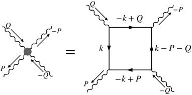
Figure 1: The effective pairing interaction for PDW bosons via exchanging fermions. In particular, $\bm{Q}$ and $\bm{P}$ in our work are related by a $\pi/2$ rotation.

Instead of keeping coefficients in the GL theory as phenomenological parameters, we determine them via integrating out fermionic degrees of freedom. The instability toward $4e$-SC can be understood as the pairing instability due to interactions among PDW bosons. While in unconventional $2e$-SC the effective interaction among fermions stems from exchanging low-energy bosons, here the effective interactions among bosons result from exchanging low-energy fermions; see Fig. 1. Importantly, we note that the form of the effective bosonic interaction is independent of the specific mechanism for PDW, and equally applies for other proposed mechanisms for PDW such as that in Ref. [37, 35]. From the effective theory, we show that $4e$-SC with $d$-wave symmetry is the dominant vestigial order. By integrating out the PDW bosons, we obtain a new effective theory for the $4e$-SC order, similar in spirit to the commonly used method for analyzing composite (vestigial) orders [42, 43, 44, 9, 45, 46, 16].

Notably, the primary PDW order parameter we consider here is multi-directional, with at least a $C_{4}$ rotation symmetry (see Fig. 2), and the PDW momenta are related by rotation. In fact, fluctuations of these PDW can lead to different composite CDW, nematic, and $4e$-SC orders. We first argue that in certain momentum space configurations $4e$-SC order is naturally favored energetically over nematic and CDW orders. Specifically, for a $C_{4}$ symmetric system, the key requirement is

$$\frac{|\bm{Q}|}{\sqrt{2}}=\big{|}\bm{k}_{F}\!\!\!\!\mod(\pi,0)\big{|},$$ (1)

where $\bm{k}_{F}$ corresponds to one of the portions on the Fermi surface that are connected by the PDW order parameters. In the next section we show several models that either automatically satisfy this condition or supports tunable $|\bm{Q}|/k_{F}$. Next we show that exchanging low-energy fermions leads to an effective interactions between PDW bosons, and the special condition (1) allows us to single out a particular interaction process that is attractive for $4e$-SC in the $d$-wave pairing channel, while repulsive in the $s$-wave channel. Furthermore, we find that this phase transition into $4e$-SC is first-order. To obtain an effective theory for the $4e$-SC order, a common approach is to do a “second” Hubbard-Stratonovich (HS) transformation (the first one referring to the process of integrating out fermions and obtaining the effective theory for PDW) to integrate out the PDW order parameters. However, the HS method, which decouples quartic interactions into bilinear terms, is inapplicable due to the higher-order terms in the PDW free energy. To address this issue, we adopt and develop a new method involving a field corresponding to the composite order parameter and an ancillary field that behaves as a Lagrange multiplier. This method bilinearizes the primary order parameters in the free energy for interactions at all orders, which can thus be integrated out, leading to an effective GL free energy for the composite order only.

We find that the first-order phase transition occurs at $T_{c}>T_{\text{PDW}}$, where $T_{\text{PDW}}$ is the onset temperature of the primary PDW order within mean-field theory. An important quantity that determines $T_{c}$ is the effective stiffness, which describes how difficult it is for the primary PDW fields to fluctuate at a given energy scale. We find that smaller stiffness yields a higher $T_{c}$. This can be understood from the fact that the composite orders are from fluctuation effect. Our theoretical treatment for $4e$-SC is based on a large-$M$ extension of the PDW effective theory, which assumes there are $M$ flavors of PDW order parameters at each momentum. This extension justifies a mean-field theory for the $4e$-SC order. Going beyond this extension, in reality we expect the $4e$-SC to occur via a Kosterlitz-Thouless transition in 2d. Despite that the transition has a different nature for $M\gg 1$ and $M=1$, it is driven by precisely the same attractive interaction we identify in this work. Depending on the number of broken symmetries, in 2d the primary PDW order may also develop a quasi-long-ranged order, but at a lower temperature.

This paper is organized as follows. In Sec. II we discuss the the PDW model as the basis for constructing composite $4e$-SC orders, and show that imposing a special condition can enhance the $4e$-SC channel. In Sec. III.1 and III.2 we show how to explicitly expand the GL free energy to higher orders in terms of the PDW fields. In Sec. III.3 we construct the free energy for the $4e$-SC orders and in Sec. III.4 study their phase transitions. Some concluding remarks are left in Sec. IV.

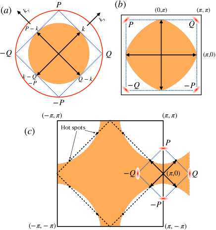
Figure 2: (a) Continuum model for PDW with $O(2)$ symmetry. The orange area is the filled Fermi sea, and the PDW momentum ${\bm{Q}}$ takes values on the Bose surface represented by the red circle. When $|{\bm{Q}}|$ equals $\sqrt{2}k_{F}$, four symmetrically distributed fermions (black arrows) can first form four symmetrically distributed PDW orders with momenta $\pm{\bm{Q}},\pm{\bm{P}}$, which then condense to give rise to $4e$-SC. (b) The PDW model realized on a square lattice when the fermions relevant for pairing are close to the van Hove points $(0,\pi)$ and $(\pi,0)$ and the PDW momentum is close to $(\pi,\pi)$. (c) PDW flucutations in the spin-fermion model. The four hot spots (black dots) near $(\pi,0)$ form a square, and the momenta for the potential PDW orders also form a square.

II Attractive interaction for $d$-wave $4e$-SC from fluctuating PDW

II.1 Microscopic models for PDW

As a starting point, we briefly review several microscopic models that hosts PDW instabilities or enhanced PDW fluctuations. One such model has been recently studied in Ref. [47]. In this model, electrons are subject to repulsive interactions, and it was found that when the local component of the interaction is suppressed and when the overall strength of the interaction exceeds some threshold value, the metallic system is susceptible towards forming PDWs instead of a uniform $2e$-SC, whose ordering vectors ${\bm{Q}}$ form a “Bose surface” in momentum space [red circle in Fig. 2(a)], and the magnitude of ${\bm{Q}}$ is mainly determined by the form of the pairing BCS interaction, and thus the ratio $\bm{q}/k_{F}$ is tunable. Here we consider a special case when,

$$|{\bm{Q}}|\approx\sqrt{2}k_{F}$$ (2)

which turns out to significantly simplify the construction of the GL free energy, as well as showing a prominent attractive interaction toward $4e$-SC.

For the lattice version of the same model, one can consider a square lattice as shown in Fig. 2(b). In this scenario, the leading instability is still toward PDWs, while the PDW ordering vectors no longer form a surface but are discretized near $(\pi,\pi)$. Interestingly, since the Fermi surface plays a more important role in choosing the ordering parameter due to anisotropy of the density of states, the PDW ordering vector and $k_{F}$ are locked such that $|{\bm{Q}}|\approx\sqrt{2}k_{F}$, where $k_{F}$ marks the position of the FS near the van Hove point, is naturally satisfied.

The relation for ${\bm{Q}}/k_{F}=\sqrt{2}$ is not specific to a particular PDW mechanism, and arises quite naturally in square lattices. For example, in the spin-fermion model for cuprates, while it has been long known that the leading instability is toward a $d$-wave $2e$-SC, PDW instabilites have also been found to exist. [37, 35] There the PDW instabilities are driven by low-energy fermions near the hotspots, and the resulting PDW ordering vectors are shown in Fig. 2 (c), and satisfy $|{\bm{Q}}|\approx\sqrt{2}|\bm{k}_{F}-(\pi,0)|$, where $\bm{k}_{F}$ is the location of a hotspot near $(\pi,0)$ . It will be straightforward to see that for our purposes, this condition is equivalent with that in Eq. (2), and for a generic $C_{4}$ symmetric system, the condition can be compactly written as that in Eq. (1).

For the remainder of our work, we take the PDW instabilities and the condition Eq. (1) as input from the microscopic model, without relying on any particular mechanism for PDW flucutations. For what we are going to do, the detailed analyses of a lattice model and a continuum model are slightly different, but the essential physics is the same. For concreteness and relevance to condensed matter systems, we will focus on the lattice version. Up to quadratic order, the Ginzburg-Landau free energy can be written as, [47]

$$F =\int\frac{d^{2}\tilde{\bm{q}}}{4\pi^{2}}\left(\frac{1}{|u(\tilde{\bm{q}})|}-\Pi_{pp}(\tilde{\bm{q}},T)\right)|{\Psi}(\tilde{\bm{q}})|^{2}~{}\text{for}~{}\tilde{\bm{q}}~{}\text{near}~{}{\bm{Q}}_{i}$$ (3)

where $u(\tilde{\bm{q}})$ is the momentum space interaction which should be attractive near the ordering momentum ${\bm{Q}}_{i}=\{\pm{\bm{P}},\pm{\bm{Q}}\}$ and we approximate it by a constant for simplicity. The pairing susceptibility $\Pi_{pp}(\tilde{\bm{q}},T)$ can be expanded near ${\bm{Q}}_{i}$ as: $\Pi_{pp}(\tilde{\bm{q}},T)\approx\nu\alpha_{0}(T)-\nu\alpha_{2}(T){\bm{q}}^{2}/k_{F}^{2}+...$, where ${\bm{q}}=\tilde{\bm{q}}-{\bm{Q}}_{i}$, $\nu$ is the density of states, and $\alpha_{0}(T)$ and $\alpha_{2}(T)$ are two dimensionless but temperature dependent coefficients. For later convenience, we rewrite Eq. (3) as

$$F=\sum_{i=\{\pm{\bm{P}},\pm{\bm{Q}}\}}\int\frac{d^{2}\bm{q}}{4\pi^{2}}\left[\alpha(T)+\kappa\bm{q}^{2}\right]\left|\Psi_{i}(\bm{q})\right|^{2}+\mathcal{O}(\Psi^{4}).$$ (4)

where $\kappa=\nu\alpha_{2}(T)/k_{F}^{2}$ is the effective stiffness for the PDW orders and since we are interested in the temperature near $T_{\text{PDW}}$ we can approximate $\kappa$ as $T$-independent. Below the mean-field transition temperature $T<T_{\rm PDW}$, $\alpha(T)<0$. We assume that $T\sim T_{\rm PDW}\ll E_{F}$ where $E_{F}$ is the Fermi energy. In general, the dispersion of the PDW bosons is anisotropic in $\bm{q}$, but as can be directly checked, for $4e$-SC instabilities the anisotropy factor can be absorbed into a redefinition of $q_{x}$ and $q_{y}$ around each PDW ordering momenta. For PDW fluctuations intrinsically driven by finite-range electronic interactions, $\kappa$ comes from both the particle-particle bubble and from the $\bm{q}$ dependence of the interaction, and for weak interactions we assume that $1/\kappa\ll{E_{F}}$. Further, as will be explained later, for analytical control of the theory, we are interested in the regime $1/\kappa\ll T_{\rm PDW}\ll{E_{F}}$. Indeed, in the microscopic theory of Ref. [47], $\kappa T_{\rm PDW}$ can be freely tuned by the interaction strength.

Below we go beyond mean-field theory for $\Psi$ and analyze the low-temperature phases.

II.2 Attractive interaction for $d$-wave $4e$-SC

The effective interaction between the PDW bosons $\Psi$ arises from exchanging fermionic degrees of freedom. As is usually done for itinerant fermions, the processes involved are described by square diagrams; see Fig. 1 for an example. The key insight here is that, for dominant four-boson interactions, the internal fermions need to come from the vicinity of the Fermi surfaces. This consideration alone singles out three types of interactions

$$\beta_{1}|\Psi_{i}|^{4}+\beta_{2}|\Psi_{\pm{\bm{P}}}|^{2}|\Psi_{\pm{\bm{Q}}}|^{2}+\beta\left(\Psi_{\bm{P}}\Psi_{-{\bm{P}}}\Psi^{*}_{\bm{Q}}\Psi^{*}_{-{\bm{Q}}}+h.c.\right),$$ (5)

where we have used the shorthands, e.g., $|\Psi_{i}|^{4}\equiv\sum_{i}\int_{\bm{q}_{1},\bm{q}_{2},\bm{q}_{3}}\Psi_{i}(\bm{q}_{1})\Psi_{i}^{*}(\bm{q}_{2})\Psi_{i}(\bm{q}_{3})\Psi_{i}^{*}(\bm{q}_{1}-\bm{q}_{2}+\bm{q}_{3})$, and $\int_{\bm{q}}\equiv\int\frac{d^{2}\bm{q}}{4\pi^{2}}$. Importantly, the last interaction with coefficient $\beta$ is of appreciable strength when the condition Eq. (1) is satisfied; otherwise at least two fermion propagators would come from regions far away from the Fermi surface.

The coefficients $\beta_{1,2}$ and $\beta$ can be readily obtained by integrating out low-energy fermions, and for $T\ll E_{F}$, we linearize the fermionic dispersion and obtain [43]

$$\beta_{1} =\frac{T}{4\pi^{2}v_{F}^{2}}\sum_{n}\int_{-E_{F}}^{E_{F}}\frac{dxdy}{(i\omega_{n}-x)^{2}(i\omega_{n}-y)^{2}}$$ (6)

$$\beta_{2} =\frac{T}{4\pi^{2}v_{F}^{2}}\sum_{n}\int_{-E_{F}}^{E_{F}}\frac{-dxdy}{(i\omega_{n}-x)^{2}(\omega_{n}^{2}+y^{2})}$$

$$\beta =\frac{T}{4\pi^{2}v_{F}^{2}}\sum_{n}\int_{-E_{F}}^{E_{F}}\frac{dxdy}{(\omega_{n}^{2}+x^{2})(\omega_{n}^{2}+y^{2})}$$

After the momentum integration and frequency summation we obtain,

$$\beta_{1}\sim\frac{1}{v_{F}^{2}E_{F}}\textrm{, }\beta_{2}\sim\frac{1}{v_{F}^{2}E_{F}}\ln\frac{E_{F}}{T}\textrm{, and }\beta=\frac{1}{16v_{F}^{2}T}.$$ (7)

Observe that $\beta\gg\beta_{1,2}$ for $T\ll E_{F}$; this can be understood from the fact that, when the dispersion is linearized and when one formally takes $E_{F}\to\infty$, both $\beta_{1,2}$ involves integrands having higher-order poles with zero residue.

Since $\beta>0$, The last term in Eq. (5) represents a repulsive for the bosons corresponding to PDW fluctuations. As is familiar from $2e$-SC, repulsive interactions may have attractive components in pairing channels with higher-angular momenta. To this end, we introduce bilinear operators $\Phi_{s}$ and $\Phi_{d}$ (not independent new fields) for $4e$-SC with $s$-wave and $d$-wave components

$$\Phi_{s}(\bm{q})\equiv \int_{\bm{p}}\Psi_{{\bm{Q}}}(\bm{p}+\bm{q})\Psi_{-{\bm{Q}}}(-\bm{p})+\Psi_{{\bm{P}}}(\bm{p}+\bm{q})\Psi_{-{\bm{P}}}(-\bm{p})$$

$$\Phi_{d}(\bm{q})\equiv \int_{\bm{p}}\Psi_{{\bm{Q}}}(\bm{p}+\bm{q})\Psi_{-{\bm{Q}}}(-\bm{p})-\Psi_{{\bm{P}}}(\bm{p}+\bm{q})\Psi_{-{\bm{P}}}(-\bm{p})$$ (8)

such that the $\beta$ interaction can be rewritten as

$$\frac{\beta}{2}\int\frac{d^{2}\bm{q}}{4\pi^{2}}|\Phi_{s}(\bm{q})|^{2}-\frac{\beta}{2}\int\frac{d^{2}\bm{q}}{4\pi^{2}}|\Phi_{d}(\bm{q})|^{2}.$$ (9)

Just like their $2e$-SC counterparts, $\Phi_{s,d}$ are distinguished by their transformation properties under the $C_{4}$ rotation: $\Phi_{s}$ is even and $\Phi_{d}$ is odd. From this decomposition it is obvious that in $d$-wave channel the charge-$4e$ pairing interaction is attractive, which can potentially lead to a $d$-wave $4e$-SC. For the $s$-wave channel, the interaction is repulsive. This is reminiscent of the situation in $2e$-SC, in that repulsive and momentum-dependent interactions can lead to Cooper pairing with higher angular momenta, most notably in the $d$-wave channel.

Before we move on to construct an effective theory for $d$-wave $4e$-SC, we comment on the other interactions and other instabilities. The $\beta_{1}$ term corresponds to a local repulsive interaction between the PDW bosons, which, if it were the only interaction, would stabilize a superfluid phase at zero temperature, i.e., the PDW phase. The $\beta_{2}$ term is repulsive, but it can be written as, up to ${\bm{P}}\to-{\bm{P}}$ and ${\bm{Q}}\to-{\bm{Q}}$,

$$\frac{\beta_{2}}{4}\left(|\Psi_{{\bm{P}}}|^{2}+|\Psi_{{\bm{Q}}}|^{2}\right)^{2}-\frac{\beta_{2}}{4}\left(|\Psi_{{\bm{P}}}|^{2}-|\Psi_{{\bm{Q}}}|^{2}\right)^{2},$$ (10)

revealing its tendency toward a nematic instability with the order parameter $\mathcal{N}\sim|\Psi_{{\bm{P}}}|^{2}-|\Psi_{{\bm{Q}}}|^{2}$. In several recent works [14, 17], it was generally found that the nematic order is more favorable compared with $4e$-SC. However, our microscopic calculation has shown that in our PDW-based model, $4e$-SC is more favored energetically, because its corresponding attraction is parametrically larger.

We also note that the decomposition of the $\beta$-term interaction is not unique. Notably, it can also be decomposed such that there is an equally attractive interaction for a charge-density-wave (CDW) composite order, with e.g., $\rho_{{\bm{P}}-{\bm{Q}}}=\Psi_{\bm{P}}\Psi^{*}_{\bm{Q}}-\Psi_{-{\bm{Q}}}\Psi^{*}_{-{\bm{P}}}$. The interplay between CDW and $4e$-SC has been systematically studied in a phenomenological model [10]. However, in our microscopic model the CDW instabilities are secondary to that of $4e$-SC. Qualitatively, the reason is the similar to the situation in a fermionic theory — in 2d and higher dimensions with weakly-coupled fermions, the CDW instability requires nesting of the Fermi surface, that is, fermionic dispersions at different momenta with a fixed difference need to be the same, while for $2e$-SC instability is guaranteed by time-reversal or inversion symmetries. Here the same reasoning holds for interacting bosons, where the bosonic dispersion for $\Psi_{{\bm{P}}}$ and $\Psi_{\bm{Q}}$ is clearly not nested. For the continuum model in Fig. 2(a), the Bose surface is not nested either. For the lattice models in Fig. 2(b,c), the lack of nesting comes from the anisotropy of the bosonic dispersion at $\pm{\bm{Q}}$ and $\pm{\bm{P}}$ illustrated by the elongated red dots. Therefore, the CDW is suppressed compared with the $d$-wave $4e$-SC, even if attractive interactions for these channels are equal.

With these considerations in mind, below we will focus on $d$-wave $4e$-SC as the sole vestigial order from the PDW fluctuations.

III Mean-field theory for $d$-wave $4e$-SC

In this section, we obtain a mean-field theory description for the transition into a $d$-wave $4e$-SC, conspired by fluctuations of the PDW bosons described by Eq. (4), and the attractive interaction in Eq. (9). In a similar spirit to the HS transformation for fermions, we integrate out the PDW bosons and obtain the free energy for the a $d$-wave $4e$-SC order parameter. Within the mean-field theory, the phase transition is then identified by a nontrivial saddle point of the free energy. Formally, the mean-field theory can be justified by extending $\Phi_{i}(\bm{q})$ at every momentum $\bm{q}$ to an $M$-component field $\Phi_{i}^{\alpha}(\bm{q})$ where $\alpha\in[1,M]$. Of course, for $M=1$, the phase transition in 2d is of Kosterlitz-Thouless nature, and the mean-field transition represents a crossover above the actual transition.

Neglecting parametrically weaker interactions $\beta_{1,2}$, and neglecting fluctuations toward $s$-wave $4e$-SC (due to the repulsive interaction they are subject to), we begin with the following free energy,

$$F= \sum_{i}\int_{\bm{q}}\left[\alpha(T)+\kappa\bm{q}^{2}\right]\left|\Psi_{i}(\bm{q})\right|^{2}-\frac{\beta}{2}\int_{\bm{q}}|\Phi_{d}(\bm{q})|^{2}+\mathcal{O}(\Psi^{6})$$ (11)

where $\Phi_{d}$ is defined in Eq. (8). The negative quartic term indicates that in a mean-field theory for PDW, the transition is first-order. When the fluctuation effects for the PDW are included, it is thus reasonable to expect that a transition into $4e$-SC is also first-order in nature. This is strongly indicated by previous analyses [42, 43], although there the free energy for the primary bosonic fields was positive-definite up to quartic order, and was truncated to quartic order. There, by a HS transformation on the primary bosonic fields, it was found that the transition into the vestigial order is first-order if the corresponding attractive interaction exceeds a threshold value.

While it is tempting to reproduce the previous analyses for quartic free energies to Eq. (11), since $F$ is unbounded at quartic level, and since higher-order terms may strongly modify a first-order transition, one needs to include higher-order interaction terms. However, unlike the quartic interaction, higher-order interaction terms cannot be decoupled using a HS transformation, and a new approaches is needed.

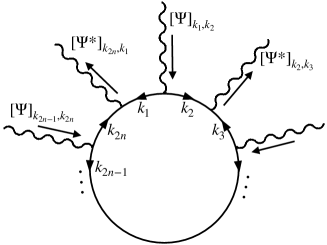
Figure 3: A general diagrammatic representation for higher-order interactions of PDW bosons.

III.1 Higher-order interaction terms

Just like the quartic interactions, higher-order interactions come microscopically from higher-order processes of exchanging low-energy fermions. Making use of the condition in Eq. (1), again only a subset of diagrams need to be included. It is easy to implement an algorithm to numerate all possible terms that satisfy the above conditions. Here we present the results, and leave technical details in Appendix A. From the 6-leg and 8-leg diagrams, the leading contributions in terms of $E_{F}/T$ at each order are

$$\gamma\left[\left(|\Psi_{{\bm{Q}}}|^{2}+|\Psi_{-{\bm{Q}}}|^{2}\right)|\Psi_{{\bm{P}}}|^{2}|\Psi_{-{\bm{P}}}|^{2}+\left(|\Psi_{{\bm{P}}}|^{2}+|\Psi_{-{\bm{P}}}|^{2}\right)|\Psi_{{\bm{Q}}}|^{2}|\Psi_{-{\bm{Q}}}|^{2}+\left(\sum_{i=1}^{4}|\Psi_{{\bm{Q}}_{i}}|^{2}\right)\left(\Psi_{{\bm{P}}}^{*}\Psi_{-{\bm{P}}}^{*}\Psi_{{\bm{Q}}}\Psi_{-{\bm{Q}}}+h.c.~{}\right)\right]$$

$$+ \frac{\zeta}{2}\left[\left(\Psi_{{\bm{P}}}^{*}\Psi_{-{\bm{P}}}^{*}\Psi_{{\bm{Q}}}\Psi_{-{\bm{Q}}}\right)^{2}+h.c.~{}\right]+4\zeta|\Psi_{{\bm{Q}}}\Psi_{-{\bm{Q}}}\Psi_{{\bm{P}}}\Psi_{-{\bm{P}}}|^{2}+\zeta\left(|\Psi_{{\bm{P}}}|^{2}|\Psi_{-{\bm{P}}}|^{2}+|\Psi_{{\bm{Q}}}|^{2}|\Psi_{-{\bm{Q}}}|^{2}\right)\left(\Psi_{{\bm{P}}}^{*}\Psi_{-{\bm{P}}}^{*}\Psi_{{\bm{Q}}}\Psi_{-{\bm{Q}}}+h.c.~{}\right)$$

$$+ \frac{\zeta}{4}\left(\sum_{i=1}^{4}|\Psi_{i}|^{4}\right)\left(\Psi_{{\bm{P}}}^{*}\Psi_{-{\bm{P}}}^{*}\Psi_{{\bm{Q}}}\Psi_{-{\bm{Q}}}+h.c.~{}\right)+\frac{\zeta}{2}\left(|\Psi_{{\bm{Q}}}|^{4}+|\Psi_{-{\bm{Q}}}|^{4}\right)|\Psi_{{\bm{P}}}|^{2}|\Psi_{-{\bm{P}}}|^{2}+\frac{\zeta}{2}\left(|\Psi_{{\bm{P}}}|^{4}+|\Psi_{-{\bm{P}}}|^{4}\right)|\Psi_{{\bm{Q}}}|^{2}|\Psi_{-{\bm{Q}}}|^{2}$$

$$+ \frac{\zeta}{2}\left(|\Psi_{{\bm{P}}}|^{2}+|\Psi_{-{\bm{P}}}|^{2}\right)\left(|\Psi_{{\bm{Q}}}|^{2}+|\Psi_{-{\bm{Q}}}|^{2}|\right)\left[|\Psi_{{\bm{P}}}|^{2}|\Psi_{-{\bm{P}}}|^{2}+|\Psi_{{\bm{Q}}}|^{2}|\Psi_{-{\bm{Q}}}|^{2}+2\left(\Psi_{{\bm{P}}}^{*}\Psi_{-{\bm{P}}}^{*}\Psi_{{\bm{Q}}}\Psi_{-{\bm{Q}}}+h.c.~{}\right)\right],$$ (12)

where the coefficients $\gamma$ and $\zeta$ are given by

$$\gamma=\frac{1}{768v_{F}^{2}}\frac{1}{T^{3}},~{}~{}~{}\zeta=\frac{1}{7680v_{F}^{2}}\frac{1}{T^{5}}.$$ (13)

Like in Eq. (5), for compactness we have suppressed the momenta carried by each fields and the integration over conserved momenta. It is straightforward to check the terms in Eq. (12) have the correct unit of energy.

Eq. (12) can be greatly simplified by using composite fields including those corresponding to $4e$-SC

$$\Psi_{{\bm{P}}}^{*}\Psi_{-{\bm{P}}}^{*}\Psi_{{\bm{Q}}}\Psi_{-{\bm{Q}}}+h.c. =\frac{1}{2}|\Phi_{s}|^{2}-\frac{1}{2}|\Phi_{d}|^{2},$$ (14)

$$|\Psi_{{\bm{P}}}|^{2}|\Psi_{-{\bm{P}}}|^{2} =\frac{1}{4}|\Phi_{s}-\Phi_{d}|^{2},$$

$$|\Psi_{{\bm{Q}}}|^{2}|\Psi_{-{\bm{Q}}}|^{2} =\frac{1}{4}|\Phi_{s}+\Phi_{d}|^{2},$$

$$\Psi_{{\bm{Q}}}\Psi_{-{\bm{Q}}}\Psi_{{\bm{P}}}\Psi_{-{\bm{P}}} =\frac{1}{16}\left(\Phi_{s}^{2}-\Phi_{d}^{2}\right)$$

$$\left(|\Psi_{{\bm{P}}}|^{2}+|\Psi_{-{\bm{P}}}|^{2}\right)\left(|\Psi_{{\bm{Q}}}|^{2}+|\Psi_{-{\bm{Q}}}|^{2}|\right) =\frac{1}{{4}}\left(\phi^{2}-\mathcal{N}^{2}\right),$$

where in the last line $\phi\equiv|\Psi_{{\bm{P}}}|^{2}+|\Psi_{-{\bm{P}}}|^{2}+|\Psi_{{\bm{Q}}}|^{2}+|\Psi_{-{\bm{Q}}}|^{2}$ is the Gaussian fluctuation and $\mathcal{N}\equiv|\Psi_{{\bm{P}}}|^{2}+|\Psi_{-{\bm{P}}}|^{2}-|\Psi_{{\bm{Q}}}|^{2}-|\Psi_{-{\bm{Q}}}|^{2}$ is the nematic order, and on both sides, the momentum dependence of the fields and the momentum integrals have been suppressed for compactness.

It is important to note that this re-expression of quartic combinations of $\Phi$ in terms of bilinear operators is not unique. For example, $|\Psi_{{\bm{P}}}|^{2}|\Psi_{-{\bm{P}}}|^{2}$ can also be rewritten as $\left[(|\Psi_{{\bm{P}}}|^{2}+|\Psi_{-{\bm{P}}}|^{2})^{2}-(|\Psi_{{\bm{P}}}|^{2}-|\Psi_{-{\bm{P}}}|^{2})^{2}\right]/4$, which does not explicitly depends on $4e$-SC flucuations. However, the re-expression can be made unique after extending the $\Psi$ field to an $M$-component $\Psi^{\alpha}$, e.g.,

$$|\Psi_{{\bm{P}}}|^{2}|\Psi_{-{\bm{P}}}|^{2} \to\frac{1}{M}\sum_{\alpha,\beta=1}^{M}\Psi_{{\bm{P}}}^{\alpha}\Psi_{{\bm{P}}}^{*\beta}\Psi_{-{\bm{P}}}^{\alpha}\Psi_{-{\bm{P}}}^{*\beta}$$

$$=\frac{M}{4}|\Phi_{s}-\Phi_{d}|^{2},$$

$$\textrm{where }\Phi_{s,d} =\frac{1}{M}\sum_{\alpha}\left(\Psi_{{\bm{Q}}}^{\alpha}\Psi_{-{\bm{Q}}}^{\alpha}\pm\Psi_{{\bm{P}}}^{\alpha}\Psi_{-{\bm{P}}}^{\alpha}\right).$$ (15)

As we will see, such a large-$M$ extension justifies the mean-field theory for $4e$-SC, and thus different extension schemes correspond to different mean-field ansatze. However, to avoid congestion of notations, we will not explicitly write the large-$M$ version of the free energy.

To arrive at a mean-field theory for $d$-wave $4e$-SC, we first take the mean-field ansatze $\mathcal{N}=\Phi_{s}=0$, that is, we neglect the nematic and $s$-wave $4e$-SC order parameters along with their fluctuations. However, note that the Gaussian fluctuation $\phi$ is always nonzero. We then have up to eighth order in $\Psi$

$${F}= \sum_{i}\int_{\bm{q}}\left[\alpha(T)+\kappa\bm{q}^{2}\right]\left|\Psi_{i}(\bm{q})\right|^{2}-\frac{\beta}{2}\int_{\bm{q}}|\Phi_{d}(\bm{q})|^{2}+$$

$$-\frac{\gamma}{4}\int_{\bm{q},\bm{p}}\Phi_{d}(\bm{q})\Phi_{d}^{*}(\bm{q}+\bm{p})\phi(\bm{p})$$

$$+\frac{\zeta}{16}\int_{\bm{q},\bm{k},\bm{p}}\Phi_{d}(\bm{q})\Phi_{d}^{*}(\bm{q}+\bm{p})\Phi_{d}(\bm{k})\Phi_{d}^{*}(\bm{k}-\bm{p})$$

$$-\frac{\zeta}{{16}}\int_{\bm{q},\bm{k},\bm{p}}\Phi_{d}(\bm{q})\Phi_{d}^{*}(\bm{q}+\bm{p})\phi(\bm{k})\phi^{*}(\bm{k}-\bm{p})+\mathcal{O}(\Psi^{10})$$ (16)

where, we remind,

$$\Phi_{d}(\bm{q})\equiv \int_{\bm{p}}\Psi_{{\bm{Q}}}(\bm{p}+\bm{q})\Psi_{-{\bm{Q}}}(-\bm{p})-\Psi_{{\bm{P}}}(\bm{p}+\bm{q})\Psi_{-{\bm{P}}}(-\bm{p})$$

$$\phi(\bm{q})\equiv \sum_{i=\pm{\bm{P}},\pm{\bm{Q}}}\int_{\bm{p}}\Psi_{i}(\bm{p}+\bm{q})\Psi_{i}^{*}(\bm{p}).$$ (17)

It is convenient at this point to measure all lengths against $n^{-1/2}$, where $n$ is electron density, and all energies against the Fermi energy, which, in lieu of a concrete fermionic model, is defined as $E_{F}\equiv v_{F}\sqrt{n}$ (i.e., we assume $n\sim k_{F}^{2}$ per Luttinger’s theorem). With these units, all parameters are made dimensionless. We have

$$\alpha= a\frac{T-T_{\rm PDW}}{T_{\rm PDW}},~{}~{}~{}\kappa\gg\frac{1}{T_{\rm PDW}}\sim\frac{1}{T}\gg 1,$$

$$\beta= \frac{1}{16T},~{}~{}\gamma=\frac{1}{768T^{3}},~{}~{}\zeta=\frac{1}{7680T^{5}}.$$ (18)

III.2 Decoupling the interaction

Here we show that the decoupling of the interaction terms at any order can be achieved by introducing two ancillary fields, one of which is a Lagrange multiplier field. Using this method, we can replace the bilinear operators $\varphi$ and $\Phi_{d}$ with local fields. For quartic interactions we show in Appendix B that the result is the same as that from the HS transformation.

We insert to the partition function the following $\delta$-function identities 

$$1 \propto\int\mathcal{D}[\lambda_{d},\Delta_{d}^{*}]\exp\left[-\frac{1}{T}\int_{\bm{q}}\lambda_{d}(\bm{q})\left({\Delta}_{d}^{*}(-\bm{q})-\Phi^{*}_{d}(\bm{q})\right)\right]$$

$$1 \propto\int\mathcal{D}[\varphi,\mu]\exp\left[-\frac{1}{T}\int_{\bm{q}}\mu(\bm{q})\left(\varphi(-\bm{q})-\phi(-\bm{q})\right)\right]$$ (19)

and the saddle points for the $\lambda$’s and $\mu$ ensures that one can replace in Eq. (16) the bilinear fluctutations $\Phi_{d}$ and $\phi$ with local fields $\Delta_{d}$ and $\varphi$. The resulting theory is

$${F}[\Psi,\Delta_{d},\varphi,\lambda_{d},\mu]$$

$$=\sum_{i}\int_{\bm{q}}\left[\alpha(T)+\kappa\bm{q}^{2}\right]\left|\Psi_{i}(\bm{q})\right|^{2}-\frac{\beta}{2}\int_{\bm{q}}|\Delta_{d}(\bm{q})|^{2}$$

$$-\frac{\gamma}{4}\int_{\bm{q},\bm{p}}\Delta_{d}(\bm{q})\Delta_{d}^{*}(\bm{q}+\bm{p})\phi(\bm{p})$$

$$+\frac{\zeta}{16}\int_{\bm{q},\bm{k},\bm{p}}\Delta_{d}(\bm{q})\Delta_{d}^{*}(\bm{q}+\bm{p})\Delta_{d}(\bm{k})\Delta_{d}^{*}(\bm{k}-\bm{p})$$

$$-\frac{\zeta}{{16}}\int_{\bm{q},\bm{k},\bm{p}}\Delta_{d}(\bm{q})\Delta_{d}^{*}(\bm{q}+\bm{p})\varphi(\bm{k})\varphi(\bm{p}-\bm{k})$$

$$+\int_{\bm{q}}\lambda_{d}(\bm{q})\left({\Delta}_{d}^{*}(\bm{q})-\Phi^{*}_{d}(\bm{q})\right)+h.c.$$

$$+\int_{\bm{q}}\mu(\bm{q})\left(\varphi(-\bm{q})-\phi(-\bm{q})\right)+\mathcal{O}(\Psi^{10})$$ (20)

where in the third line we deliberately do not replace $\phi(\bm{p})$ with $\varphi(\bm{p})$.

As a mean-field ansatz, we consider saddle-point solutions of the composite fields that are spatially uniform, with $\Delta_{d}(\bm{q})=\Delta_{d}\delta(\bm{q})$, and $\varphi(\bm{q})=\varphi\delta(\bm{q})$. Using the regularization $\delta(\bm{q}=0)=V$ where $V$ is the volume (area) of the system and defining the free energy density $\mathcal{F}\equiv F/V$, Eq. (20) then becomes

$$\mathcal{F}[\Psi,\Delta_{d},\varphi,\lambda_{d},\mu)$$

$$=\sum_{i,\bm{q}}\left[\alpha(T)+\kappa\bm{q}^{2}-\frac{\gamma}{4}|\Delta_{d}|^{2}-\mu\right]\left|\Psi_{i}(\bm{q})\right|^{2}$$

$$-\frac{\beta}{2}|\Delta_{d}|^{2}+\frac{\zeta}{16}|\Delta_{d}|^{4}-\frac{\zeta}{{16}}|\Delta_{d}|^{2}\varphi^{2}$$

$$+\lambda_{d}\left({\Delta}_{d}^{*}-\Phi^{*}_{d}\right)+\lambda_{d}^{*}\left({\Delta}_{d}-\Phi_{d}\right)+\mu\varphi+\mathcal{O}(\Psi^{10}),$$ (21)

where $\lambda_{d}\equiv\lambda_{d}(\bm{q}=0)/V$, $\mu\equiv\mu(\bm{q}=0)/V$, and we have used the fact that ${V}\int_{\bm{q}}\equiv\sum_{\bm{q}}$ in the continuum limit.

III.3 Free energy for $d$-wave $4e$-SC

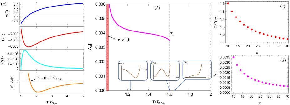
Figure 4: Numerical results for the phase transition of $\Delta_{d}$. (a) The GL coefficients $A(T)$, $B(T)$ and $C(T)$ in Eq.(31) obtained for taking $a=10^{-3},T_{\text{PDW}}=0.1$ and $\kappa=10$. The $\Delta_{d}\neq 0$ phase transition temperature $T_{c}$ is determined by the condition $B^{2}-4AC=0$. (b) The $4e$-SC order parameter as a function of $T$. For clarity we also show the free energy profile at different $T$ as the insets. The pink colored region at $T$ close to $T_{\text{PDW}}$ is where $r<0$ and our perturbative analysis breaks down due to a large $|\Delta_{d}|$. (c) and (d), $T_{c}$ and $|\Delta_{d}|$ at $T_{c}$ as a function of the effective stiffness $\kappa$.

To justify a mean-field theory, we formally extend Eq. (16) to a large-$M$ version using the scheme described in Eq. (15). Together with rescaling $\lambda_{d}\to M\lambda_{d}$ and $\mu\to M\mu$, Eq. (21) becomes

$$\mathcal{F}[\Psi,\Delta_{d},\varphi,\lambda_{d},\mu)$$ (22)

$$=\sum_{j=1}^{M}\sum_{i}\int_{\bm{q}}\left[\alpha(T)+\kappa\bm{q}^{2}-\frac{\gamma}{4}|\Delta_{d}|^{2}-\mu\right]\left|\Psi_{i}^{j}(\bm{q})\right|^{2}$$

$$-\frac{M\beta}{2}|\Delta_{d}|^{2}+\frac{M\zeta}{16}|\Delta_{d}|^{4}-\frac{M\zeta}{{16}}|\Delta_{d}|^{2}\varphi^{2}$$

$$+M\lambda_{d}\left({\Delta}_{d}^{*}-\Phi^{*}_{d}\right)+M\lambda_{d}^{*}\left({\Delta}_{d}-\Phi_{d}\right)+M\mu\varphi+\mathcal{O}(\Psi^{10}).$$

Since $\mathcal{F}$ is quadratic in $\Psi$, we can integrate it out. We get, up to higher-order terms

$$\mathcal{F}(\Delta_{d},\varphi,\lambda_{d},\mu)/M$$

$$= {2}T\int_{\bm{q}}\ln\left[(\alpha(T)+\kappa\bm{q}^{2}-\frac{\gamma}{4}|\Delta_{d}|^{2}-\mu)^{2}-|\lambda_{d}|^{2}\right]$$

$$-\frac{\beta}{2}|\Delta_{d}|^{2}+\frac{\zeta}{16}|\Delta_{d}|^{4}-\frac{\zeta}{{16}}|\Delta_{d}|^{2}\varphi^{2}$$

$$+\lambda_{d}{\Delta}_{d}^{*}+\lambda_{d}^{*}{\Delta}_{d}+\mu\varphi,$$ (23)

where the upper cutoff is a proper combination of high-energy scale $E_{F}$ and short distance scale $n^{-1/2}$, which in our units is 1. We have also used $\frac{1}{V}\sum{\bm{q}}\equiv\int_{\bm{q}}$.

In the $M\to\infty$ limit, the partition function $Z=e^{-\mathcal{F}V/T}$ is completely determined by the saddle points of $\Delta_{d},\varphi,\lambda_{d}$ and $\mu$. One can take the saddle-point equations to eliminate the Lagrange multiplier fields $\lambda_{d}$ and $\mu$. We get from the requirements $\partial\mathcal{F}/\partial\varphi=0$, $\partial\mathcal{F}/\partial\lambda_{d}^{*}=0$ and $\partial\mathcal{F}/\partial\mu=0$ that

$$\mu= \frac{\zeta}{{8}}|\Delta_{d}|^{2}\varphi$$ (24)

$$|\lambda_{d}|= r\tanh\frac{{2}\pi\kappa|\Delta_{d}|}{T}$$ (25)

$$\varphi= \frac{T}{\pi\kappa}\ln\left(\frac{{\kappa}}{r}\cosh\frac{{2}\pi\kappa|\Delta_{d}|}{T}\right),$$ (26)

$$\textrm{where }r\equiv \alpha(T)-\frac{\gamma}{{4}}|\Delta_{d}|^{2}-\frac{\zeta}{{8}}|\Delta_{d}|^{2}\varphi.$$ (27)

Note that in order to legitimize the procedure of integrating out PDW orders, we need to keep $r$ as positive definite. This will be justified in our following calculation for $\Delta_{d}$. Eqs. (24, 25) can be used to eliminate the Lagrange multiplier fields $\lambda$ and $\mu$ in Eq. (23), which yields

$$\frac{\mathcal{F}(\Delta_{d})}{M}=-\frac{\beta}{2}|\Delta_{d}|^{2}+\frac{\zeta}{16}|\Delta_{d}|^{4}+\frac{\zeta}{16}|\Delta_{d}|^{2}\varphi^{2}+r\varphi+\frac{rT}{\pi\kappa}$$

$$=\alpha(T)\varphi-\left(\frac{\beta}{2}+\frac{T\gamma}{4\pi\kappa}\right)|\Delta_{d}|^{2}-\left(\frac{\gamma}{4}+\frac{T\zeta}{8\pi\kappa}\right)|\Delta_{d}|^{2}\varphi$$

$$-\frac{\zeta}{16}|\Delta_{d}|^{2}\varphi^{2}+\frac{\zeta}{16}|\Delta_{d}|^{4}+\rm{const},$$ (28)

where at the second equality we have used Eq. (27) to eliminate $r$.

The $\varphi$ dependence in Eq. (28) can be further eliminated using Eq. (26), which does not admit a closed-form solution but can be expressed in Taylor expansion

$$\varphi=\frac{T}{\pi\kappa}\ln\frac{\kappa}{\alpha}+c_{2}|\Delta_{d}|^{2}+c_{4}|\Delta_{d}|^{4}+c_{6}|\Delta_{d}|^{6}+...$$ (29)

where the first term is the familiar logarithmic divergence of Gaussian fluctuations in 2d, and the rest is the back action from $4e$-SC fluctuations. Substituting this expansion into Eq. (26) and matching the coefficients on both sides, we find, omitting high-order terms in $c_{6}$ due to space,

$$c_{2} =\frac{2\pi\kappa}{T}+\frac{\gamma T}{4\pi\alpha\kappa}+\frac{\zeta T^{2}}{8\pi^{2}\alpha\kappa^{2}}\ln\frac{\kappa}{\alpha},$$ (30)

$$c_{4} =-\frac{4\pi^{3}\kappa^{3}}{3T^{3}}+\frac{\zeta}{4\alpha}+\frac{\gamma^{2}T}{32\pi\alpha^{2}\kappa}+\frac{\gamma\zeta T^{2}}{32\pi^{2}\alpha^{2}\kappa^{2}}\ln\frac{\kappa}{\alpha}$$

$$~{}~{}+\frac{\zeta^{2}T^{3}}{64\pi^{3}\alpha^{2}\kappa^{3}}\ln\frac{\kappa}{\alpha}+\frac{\zeta^{2}T^{3}}{128\pi^{3}\alpha^{2}\kappa^{3}}\ln^{2}\frac{\kappa}{\alpha}$$

$$c_{6} =\frac{64\pi^{5}\kappa^{5}}{45T^{5}}-\frac{\pi^{2}\zeta\kappa^{2}}{6\alpha T^{2}}+\cdots$$

As a result, we have, after dropping the constant terms

$$\frac{\mathcal{F}(\Delta_{d})}{M}=A(T)|\Delta_{d}|^{2}+B(T)|\Delta_{d}|^{4}+C(T)|\Delta_{d}|^{6}+\cdots$$ (31)

where the Ginzburg-Landau coefficients are

$$A(T) =\frac{2\pi\alpha\kappa}{T}-\frac{\beta}{2}-\frac{\gamma T}{4\pi\kappa}\ln\frac{\kappa}{\alpha}-\frac{\zeta T^{2}}{16\pi^{2}\kappa^{2}}\ln^{2}\frac{\kappa}{\alpha},$$ (32)

$$B(T) =-\frac{4\pi^{3}\alpha\kappa^{3}}{3T^{3}}-\frac{\pi\gamma\kappa}{2T}+\frac{\zeta}{16}-\frac{\gamma^{2}T}{32\pi\alpha\kappa}$$

$$-\frac{\zeta}{4}\left(\frac{\gamma T^{2}}{8\pi^{2}\alpha\kappa^{2}}+1\right)\ln\frac{\kappa}{\alpha}-\frac{\zeta^{2}T^{3}}{128\pi^{3}\alpha\kappa^{3}}\ln^{2}\frac{\kappa}{\alpha},$$

$$C(T) =\frac{64\pi^{5}\alpha\kappa^{5}}{45T^{5}}+\frac{\pi^{3}\gamma\kappa^{3}}{3T^{3}}+\frac{\pi^{2}\zeta\kappa^{2}}{6T^{2}}\left(\ln\frac{\kappa}{\alpha}-\frac{3}{2}\right)+\cdots$$

Using Eq. (18), we see that all terms in Eq. (32), are actually organized in increasing powers of $1/\kappa T\ll 1$ or $1/\kappa\alpha$. Assuming $\kappa\alpha\gtrsim 1$ as we will justify below, the coefficients can be greatly simplified. Indeed, we have already omitted many terms in higher powers of $1/\kappa T$ in $C(T)$. More importantly, higher-order terms in the PDW field $\Psi$ in Eq. (16) in fact enter all coefficients $A$, $B$, and $C$, but it is straightforward to see from the pattern that they are further suppressed by $1/\kappa T$. In this sense, the expressions in Eq. (32) only make sense in the $\kappa T\gg 1$ limit. We have

$$A(T)\approx \frac{2\pi\alpha\kappa}{T}-\frac{\beta}{2}$$

$$B(T)\approx -\frac{4\pi^{3}\alpha\kappa^{3}}{3T^{3}}-\frac{\pi\gamma\kappa}{2T}$$

$$C(T)\approx \frac{64\pi^{5}\alpha\kappa^{5}}{45T^{5}}+\frac{\pi^{3}\gamma\kappa^{3}}{3T^{3}}.$$ (33)

In the opposite limit $\kappa T\ll 1$, the effective theory for PDW bosons becomes strongly coupled, and a perturbative expansion in $\Psi$ becomes inadequate.

III.4 Mean-field transition into $d$-wave $4e$-SC

Driven by the temperature dependence of $\alpha(T)$, the quadratic coefficient $A(T)$ becomes negative upon lowering temperature when $\alpha\kappa=\beta T/4\pi\approx 0.005$. As this point, we see that $B(T)<0$, i.e., $\Delta_{d}=0$ is no longer a local minimum of the free energy. Instead, the global minimum of free energy is given by $\Delta_{d}\neq 0$. Therefore, a first-order phase transition must have already occurred at a higher temperature. The transition temperature is determined by the condition $B^{2}\sim AC$, and thus we find by using Eq. (18) that

$$\alpha_{c}\sim 1/\kappa,~{}~{}~{}T_{c}>T_{\rm PDW}.$$ (34)

and that at the onset,

$$|\Delta_{d}|^{2}\sim\frac{T_{c}^{2}}{\kappa^{2}}.$$ (35)

We see that a smaller stiffness term $\kappa$ leads to a higher $T_{c}$ and a larger onset for $\Delta_{d}$. This is the main conclusion of this work.

One important consistency check for our theory is that $r$ defined in Eq. (27) should be positive, at least until the phase transition occurs. Plugging Eq. (35) and Eq. (29) into Eq. (27) we see that at the transition $r\approx\alpha$, which is indeed positive. Taking Eq. (31) at face value, the first-order phase transition occurs when $B^{2}=4AC$. However, we caution that with a truncation at finite order, the free energy (31) is unreliable in quantitatively determining a first-order transition temperature, as higher-order terms are equally important. Nevertheless, the qualitative relations (34, 35) remain valid even in the presence of higher-order terms.

It is important here to note that within the large-$M$ theory, the mean-field temperature $T_{\rm PDW}$ should not be identified as the transition temperature into a PDW state. In fact, with $M$ components, the $\Psi_{i}^{\alpha}$ field can never condense at any finite temperature. Instead, within the large-$M$ framework, a PDW state should be recognized as a state in which both $U(1)$ and translational symmetries are broken, e.g., with both $\langle\Phi_{d}\rangle\neq 0$ and $\langle\rho_{\bm{p}-\bm{q}}\rangle\neq 0$. As we discussed, however, the $4e$-SC order is by far the predominant one, and translational symmetry remains intact well into the $4e$-SC state. Therefore, the PDW order can only develop at much lower temperatures if at all. Similarly for $M=1$, the $4e$-SC state has quasi-long-range order via a Kosterlitz-Thouless transition, and PDW state may only develop via another Kosterlitz-Thouless transition at lower temperatures corresponding to the translation symmetry.

Complementary to the analytical approach, we also solved numerically for saddle points using the full expressions in Eqs. (31, 32). In Fig. 4(a) we show the temperature dependence of the GL coefficients $A,B$ and $C$, together with the quantity $B^{2}-4AC$, for a typical set of parameters $a=10^{-3}$, $T_{\text{PDW}}=0.1$ and $\kappa=10$. We see clearly that above $T_{\text{PDW}}$, $B$ remains negative while $C$ remains positive. $A$ changes sign at some particular $T$, which is consistent with our above analysis and can be also seen from the leading approximation in Eq. (33). The quantity $B^{2}-4AC$ vanishes as $T\to T_{c}$, and thus can be used to obtain $T_{c}$. For this particular set of parameters, we obtain that $T_{c}\approx 1.6T_{\text{PDW}}$. In Fig. 4(b) we show the magnitude of the $d$-wave $4e$-SC order parameter $|\Delta_{d}|$ as a function of $T$, which is calculated via

$$|\Delta_{d}|=\left(\frac{-B+\sqrt{B^{2}-3AC}}{3C}\right)^{1/2}$$ (36)

for $B<0$ and $C>0$ is always satisfied near $T_{c}$. We see that $|\Delta_{d}|$ increases monotonically as $T$ decreases below $T_{c}$. From Eq. (27) we see that once $|\Delta_{d}|$ becomes large enough, $r$ will eventually becomes negative, invalidating our perturbative analysis. In practice, in the region of $r<0$ one needs to keep expanding to higher orders of the PDW order parameters. We also show the free energy profile for $T>T_{c}$, $T=T_{c}$ and $T<T_{c}$, from which the nature of first order phase transition is seen directly. In order to show the impact of the stiffness $\kappa$ on various quantities for the $4e$-SC order, we show in Fig. 4(c) and (d) the plot of $T_{c}$ and $|\Delta_{d}(Tc)|$ as a function of $\kappa$. It is clear that a larger $\kappa$ yields a smaller $T_{c}$ and $|\Delta_{d}(T_{c})|$. This is consistent with Eq. (35), although that is obtained in the limit that $\kappa T\gg 1$.

IV Conclusion and outlook

In this work, we studied the phase transition driven by bidirectional fluctuations of PDWs. We showed that when the ratio of PDW momenta and the Fermi momenta is $\sqrt{2}$, the predominant interaction among PDW bosons is attractive in the $d$-wave pairing channel of the PDW bosons. In contrast to earlier works, such a $4e$-SC state is the leading vestigial instability of $2e$-SC fluctuations. The $d$-wave nature is reminiscent of $d$-wave $2e$-SC in fermionic pairing problems with repulsive interactions. Interestingly, we found that the similar pairing mechanism can be applied to the formation of $4e$-SC.

On the technical level, we developed a new formalism to analyze vestigial orders. Earlier works [42, 43] analyzed the free energy of primary orders that is bounded up to quartic order and used a HS transformation to decouple the four-boson interactions. In this work we have an unbounded free energy of PDW bosons that calls for the inclusion higher-order bosonic interactions. We introduced Langrange multiplier fields which enable us to decouple interactions any other order. As a result, we found that the transition into the $d$-wave $4e$-SC is weakly first-order with a higher transition temperature than the mean-field $T_{\rm PDW}$.

Our theory has interesting implications for unconventional superconductors. There exist strong evidence for PDW in underdoped cuprates, although it is likely unidirectional within each Cu-O plane and alters between $x$ and $y$ ordering direction between neighboring planes [44]. Our work points to a possibility of $4e$-SC with a relative sign change between neighboring Cu-O planes with perpendicular PDW wavevectors, although microscopic details call for a separate analysis. In addition, both PDW and $4e$-SC (and $6e$-SC) have been proposed to exist in the Kagome metal CsV₃Sb₅[49, 50, 51]. It would be interesting to generalize our theory to hexagonal systems, which may be applied to CsV₃Sb₅. Finally, the mean-field theory developed here for $4e$-SC can be directly tested using unbiased numerical methods such as quantum Monte Carlo simulations, which we leave as future work.

Note added: During the preparation of the manuscript, we became aware of a recent work Ref. [17] by Hecker et al., in which $d$-wave $4e$-SC was considered as a vestigial order of a two-component superconductor. Different from our work, the $d$-wave $4e$-SC was found to be a subleading instability.

Appendix A Details of finding leading contributions up to $\mathcal{O}(|\Psi|^{8})$

In obtaining the Ginzburg-Landau theory for the primary PDW orders, we integrate out the fermions and obtain

$$-\text{tr}\ln\mathcal{G}^{-1}$$ (37)

in the action. The matrix $\mathcal{G}$ is defined as $\mathcal{G}^{-1}=G_{0}^{-1}+\hat{\Delta}$ and

$$G_{0}^{-1}=\begin{pmatrix}G_{p}^{-1}&0\\ 0&G_{h}^{-1}\end{pmatrix},~{}~{}~{}\hat{\Delta}=\begin{pmatrix}0&\Psi\\ \Psi^{\dagger}&0\end{pmatrix}$$ (38)

The particle and hole Green’s function $G_{p}$ and $G_{h}$ are diagonal in frequency-momentum space. For instance, $[G_{p}]_{k,k^{\prime}}=G_{p}(k)\delta_{k,k^{\prime}}$. While $\Psi$ and $\Psi^{\dagger}$ is not diagonal in momentum space. In particular, we have $[\Psi]_{k,k^{\prime}}=\sum_{i}\Psi_{{\bm{Q}}_{i}}\delta_{k,{\bm{Q}}_{i}-k^{\prime}}$ and $[\Psi^{\dagger}]_{k,k^{\prime}}=\sum_{i}\Psi^{\dagger}_{{\bm{Q}}_{i}}\delta_{k,-{\bm{Q}}_{i}-k^{\prime}}$ with ${\bm{Q}}_{i}\in\{\pm{\bm{Q}},\pm{\bm{P}}\}$. Expanding Eq. (37) in terms of $\Psi_{{\bm{Q}}_{i}}$, we obtain

$$-\text{tr}\ln\mathcal{G}^{-1} =-\text{tr}\ln G_{0}^{-1}-\text{tr}\ln(1+G_{0}\hat{\Delta})$$ (39)

$$=-\text{tr}\ln G_{0}^{-1}+\sum_{n=1}^{\infty}\frac{1}{2n}\text{tr}(G_{0}\hat{\Delta})^{2n}.$$

Given the matrix structure in Eq. (38), it is easy to see that $G_{0}$ is can be obtained by simply taking the inverse of the diagonal elements of $G_{0}^{-1}$. The $n$-th element in the series is given by

$$\frac{1}{2n}\sum_{\{k_{i}\}} [G_{p}]_{k_{1}}[\Psi]_{k_{1},k_{2}}[G_{h}]_{k_{2}}[\Psi^{*}]_{k_{2},k_{3}}...$$ (40)

$$...[G_{p}]_{k_{2n-1}}[\Psi]_{k_{2n-1},k_{2n}}[G_{h}]_{k_{2n}}[\Psi^{*}]_{k_{2n},k_{1}}$$

In our special situation, all the Green’s functions should be $G_{i},i=1,...,4$, which are

$$G_{1}(k)=\frac{1}{i\omega_{n}-v_{F}k_{x}},G_{2}(k)=\frac{-1}{i\omega_{n}-v_{F}k_{y}},$$ (41)

$$G_{3}(k)=\frac{1}{i\omega_{n}+v_{F}k_{x}},G_{4}(k)=\frac{-1}{i\omega_{n}+v_{F}k_{y}}.$$

Given a set of Green’s functions, the external momentum can be determined by momentum conservation. Therefore, each diagram uniquely corresponds to one permutation of the Green’s function set. We can develop a simple algorithm to numerate all the possible combinations for any $n$ based on Eq. (40). The algorithm processes as follows,

1. For a given $n$, specify all possible set $S$ for $2n$ Green’s functions that satisfy the momentum conservation rule. For instance, for $n=2$, one possible set is $S=\{1,2,3,4\}$, meaning all the leading contributions corresponds to all the permutations of this set.

2. Generate all possible permutations for the set $S$, and keep only those nonequivalent ones.

3. Identify external legs for each nonequivalent permutations based on momentum conservation.

4. collect all the terms from different permutations for a given set, repeat the procedure for all sets.

Below we briefly discuss how to obtain (12). For $n=3$, the internal Green’s functions runs over the set $\{1,2,3,4,1,2\}$, where we denote $G_{i}$ by $i$ for brevity. Note that the set is equivalent to $\{1,2,3,4,2,3\}$, $\{1,2,3,4,3,4\}$ and $\{1,2,3,4,4,1\}$ by $D_{4}$ symmetry. Thus all of these sets should be considered, and they combined to give the $\gamma$ terms in Eq. (12).

The results for $n=4$ contains more terms. First of all, all the fermion Green’s functions can run over the set $\{1,2,3,4,1,2,3,4\}$. The set is invariant under $D_{4}$ group operation so this is a complete class. The momentum integral yields a factor of $\zeta$ for this class, and this is presented in the second line of Eq. (12). The second class comes from the set $\{1,2,3,4,1,1,2,2\}$ and its symmetry related ones $\{1,2,3,4,2,2,3,3\}$, $\{1,2,3,4,3,3,4,4\}$ and $\{1,2,3,4,4,4,1,1\}$. The one-loop integral for these diagrams leads to a factor of $\zeta/4$, and this class corresponds to the third line of Eq. (12). The last class comes from the set $\{1,2,3,4,1,1,2,4\}$, $\{1,2,3,4,2,2,1,3\}$, $\{1,2,3,4,3,3,2,4\}$ and $\{1,2,3,4,4,4,1,3\}$, for which the one-loop integral yields a factor of $\zeta/2$. This corresponds to the last line of Eq. (12). It can be checked that all other sets doest not meet the momentum conservation, i.e. they will lead to some external legs for which the momentum is neither $\pm{\bm{Q}}$ nor $\pm{\bm{P}}$. Therefore, Eq. (12) is all the leading contributions at $\mathcal{O}(|\Psi_{{\bm{Q}}_{i}}|^{8})$.

Appendix B Equivalence between HS transformation and the method of using Lagrangian multiplier

In a special case when $\gamma$ and $\zeta$ terms are absent from the action, one can alternatively perform HS (HS) transformation to analyze the charge-$4e$ order. Below we show that the HS transformation yields exactly the same results as we obtain by using Lagrangian multiplier. The action we consider is

$$\int\frac{d^{2}q}{4\pi^{2}}\left[(\kappa q^{2}+\alpha)\sum_{i=1}^{4}|\Psi_{{\bm{Q}}_{i}}|^{2}\right]-\frac{\beta}{2}|\Phi_{d}|^{2}$$ (42)

with $\beta>0$. After HS transformation, the action becomes

$$\frac{\beta}{2}\left(|\Delta_{d}|^{2}-\Delta_{d}{\Phi_{d}}^{*}-\bar{\Delta}_{d}\Psi_{d}\right)+\int\frac{d^{2}q}{4\pi^{2}}\left[(\kappa q^{2}+\alpha)\sum_{i=1}^{4}|\Psi_{{\bm{Q}}_{i}}|^{2}\right]$$ (43)

Again one can integrate out the PDW order parameters using the basis $\Psi=(\Psi_{{\bm{Q}}},\Psi_{{\bm{P}}},\Psi^{\dagger}_{-{\bm{Q}}},\Psi^{\dagger}_{-{\bm{P}}})^{T}$. This leads to the following effective action for the charge-$4e$ order

$$\frac{\beta}{2}\Delta_{d}^{2}+T\int\frac{d^{2}q}{4\pi^{2}}\text{tr}\ln A(q)$$ (44)

where

$$A(q)=\begin{pmatrix}\kappa q^{2}+\alpha&0&-\frac{\beta}{2}\Delta_{d}&0\\ 0&\kappa q^{2}+\alpha&0&\frac{\beta}{2}\Delta_{d}\\ -\frac{\beta}{2}\bar{\Delta}_{d}&0&\kappa q^{2}+\alpha&0\\ 0&\frac{\beta}{2}\bar{\Delta}_{d}&0&\kappa q^{2}+\alpha\end{pmatrix}.$$ (45)

Performing the tr$\ln$ operation, Eq. (37) becomes

$$\frac{\beta}{2}\Delta_{d}^{2}+T\int\frac{d^{2}q}{2\pi^{2}}\ln\left[(\kappa q^{2}+\alpha)^{2}-\frac{\beta^{2}}{4}\Delta_{d}^{2}\right]$$ (46)

The saddle point of this action reads

$$1 ={\beta}T\int\frac{d^{2}q}{4\pi^{2}}\frac{1}{(\kappa q^{2}+\alpha)^{2}-\frac{\beta^{2}}{4}\Delta_{d}^{2}}$$ (47)

$$=\frac{\beta T}{4\pi\kappa}\frac{1}{\frac{\beta}{2}\Delta_{d}}\text{arccoth}\frac{\alpha}{\frac{\beta}{2}\Delta_{d}},$$

or equivalently,

$$\Delta_{d}=\frac{T}{2\pi\kappa}\text{arccoth}\frac{2\alpha}{\beta\Delta_{d}}~{}~{}\text{or}~{}~{}\tanh(2\pi\kappa\Delta_{d}/T)=\frac{\beta\Delta_{d}}{2\alpha}.$$ (48)

In obtaining the above saddle point equations, we have used the condition that $\alpha>\frac{\beta}{2}\Delta_{d}$, as is required for the convergence of the Gaussian integral in order to integrate out PDW fields. Eq. (48) is the results obtained via HS transformation at quartic level.

To compare Eq. (48) with the one obtained using the method of Lagrangian multiplier, we note from Eq. (26) that in the absence of $\gamma$ and $\zeta$, we have

$$\varphi=\frac{T}{\pi\kappa}\ln\left(\frac{{\kappa}}{\alpha}\cosh\frac{{2}\pi\kappa|\Delta_{d}|}{T}\right).$$ (49)

The free energy for $\Delta_{d}$ then becomes

$$\!\!\!\!\!\!\!\!\!\!\!\!\mathcal{F}[\Delta_{d}]=-\frac{\beta}{2}|\Delta_{d}|^{2}+\frac{\alpha T}{\pi\kappa}\left[1+\ln\left(\frac{{\kappa}}{\alpha}\cosh\frac{{2}\pi\kappa|\Delta_{d}|}{T}\right)\right].$$ (50)

Variation of this free energy with respect to $|\Delta_{d}|$ and set it to zero, we immediately obtain the gap equation

$$-\frac{\beta}{2}\Delta_{d}+\alpha\tanh(2\pi\kappa\Delta_{d}/T)=0$$ (51)

which is exactly the same as Eq. (48). Therefore, we have proved that at the level of $\mathcal{O}(\Psi^{4})$, both the HS transformation and the method of Lagrangian multiplier yield the same result. However, the HS transformation, which is built on Gaussian integral, fails to work once higher order terms of the primary order parameters are included, but the Lagrangian multiplier method is still valid.

References

- Röpke et al. [1998] G. Röpke, A. Schnell, P. Schuck, and P. Nozières, Four-particle condensate in strongly coupled fermion systems, Phys. Rev. Lett. 80, 3177 (1998).
- Wu [2005] C. Wu, Competing orders in one-dimensional spin- fermionic systems, Phys. Rev. Lett. 95, 266404 (2005).
- Aligia et al. [2005] A. A. Aligia, A. P. Kampf, and J. Mannhart, Quartet formation at interfaces of -wave superconductors, Phys. Rev. Lett. 94, 247004 (2005).
- Herland et al. [2010] E. V. Herland, E. Babaev, and A. Sudbø, Phase transitions in a three dimensional lattice london superconductor: Metallic superfluid and charge- superconducting states, Phys. Rev. B 82, 134511 (2010).
- Moon [2012] E.-G. Moon, Skyrmions with quadratic band touching fermions: A way to achieve charge superconductivity, Phys. Rev. B 85, 245123 (2012).
- Ge et al. [2022] J. Ge, P. Wang, Y. Xing, Q. Yin, H. Lei, Z. Wang, and J. Wang, Discovery of charge-4e and charge-6e superconductivity in kagome superconductor csv3sb5 10.48550/ARXIV.2201.10352 (2022).
- Gnezdilov and Wang [2022] N. V. Gnezdilov and Y. Wang, Solvable model for a charge- superconductor, Phys. Rev. B 106, 094508 (2022).
- Jiang et al. [2017] Y.-F. Jiang, Z.-X. Li, S. A. Kivelson, and H. Yao, Charge- superconductors: A majorana quantum monte carlo study, Phys. Rev. B 95, 241103 (2017).
- Fradkin et al. [2015] E. Fradkin, S. A. Kivelson, and J. M. Tranquada, Colloquium: Theory of intertwined orders in high temperature superconductors, Rev. Mod. Phys. 87, 457 (2015).
- Berg et al. [2009a] E. Berg, E. Fradkin, and S. A. Kivelson, Charge-4e superconductivity from pair-density-wave order in certain high-temperature superconductors, Nature Physics 5, 830 (2009a).
- Radzihovsky and Vishwanath [2009] L. Radzihovsky and A. Vishwanath, Quantum liquid crystals in an imbalanced fermi gas: Fluctuations and fractional vortices in larkin-ovchinnikov states, Phys. Rev. Lett. 103, 010404 (2009).
- Agterberg et al. [2011] D. F. Agterberg, M. Geracie, and H. Tsunetsugu, Conventional and charge-six superfluids from melting hexagonal fulde-ferrell-larkin-ovchinnikov phases in two dimensions, Phys. Rev. B 84, 014513 (2011).
- Agterberg and Tsunetsugu [2008] D. F. Agterberg and H. Tsunetsugu, Dislocations and vortices in pair-density-wave superconductors, Nature Physics 4, 639 (2008).
- Fernandes and Fu [2021] R. M. Fernandes and L. Fu, Charge- superconductivity from multicomponent nematic pairing: Application to twisted bilayer graphene, Phys. Rev. Lett. 127, 047001 (2021).
- Jian et al. [2021] S.-K. Jian, Y. Huang, and H. Yao, Charge- superconductivity from nematic superconductors in two and three dimensions, Phys. Rev. Lett. 127, 227001 (2021).
- Poduval and Scheurer [2023] P. P. Poduval and M. S. Scheurer, Vestigial singlet pairing in a fluctuating magnetic triplet superconductor: Applications to graphene moiré systems. arxiv.2301.01344 (2023).
- Hecker et al. [2023] M. Hecker, R. Willa, J. Schmalian, and R. M. Fernandes, Cascade of vestigial orders in two-component superconductors: nematic, ferromagnetic, s-wave charge-4e, and d-wave charge-4e states. arxiv:2303.00653 (2023), arXiv:2303.00653 [cond-mat.supr-con] .
- Agterberg et al. [2020] D. F. Agterberg, J. S. Davis, S. D. Edkins, E. Fradkin, D. J. Van Harlingen, S. A. Kivelson, P. A. Lee, L. Radzihovsky, J. M. Tranquada, and Y. Wang, The physics of pair-density waves: Cuprate superconductors and beyond, Annual Review of Condensed Matter Physics 11, 231 (2020).
- Fulde and Ferrell [1964] P. Fulde and R. A. Ferrell, Superconductivity in a strong spin-exchange field, Phys. Rev. 135, A550 (1964).
- Larkin and Ovchinnikov [1965] A. I. Larkin and Y. N. Ovchinnikov, Nonuniform state of superconductors, Sov. Phys. JETP 20, 762 (1965).
- Agosta [2018] C. C. Agosta, Inhomogeneous superconductivity in organic and related superconductors, Crystals 8, 285 (2018).
- Matsuda and Shimahara [2007] Y. Matsuda and H. Shimahara, Fulde–ferrell–larkin–ovchinnikov state in heavy fermion superconductors, Journal of the Physical Society of Japan 76, 051005 (2007).
- Gurevich [2010] A. Gurevich, Upper critical field and the fulde-ferrel-larkin-ovchinnikov transition in multiband superconductors, Phys. Rev. B 82, 184504 (2010).
- Cho et al. [2017] C.-w. Cho, J. H. Yang, N. F. Q. Yuan, J. Shen, T. Wolf, and R. Lortz, Thermodynamic evidence for the fulde-ferrell-larkin-ovchinnikov state in the superconductor, Phys. Rev. Lett. 119, 217002 (2017).
- Liu et al. [2021] X. Liu, Y. X. Chong, R. Sharma, and J. C. S. Davis, Discovery of a cooper-pair density wave state in a transition-metal dichalcogenide, Science 372, 1447 (2021).
- Wu et al. [2023a] Y.-M. Wu, Z. Wu, and H. Yao, Pair-density-wave and chiral superconductivity in twisted bilayer transition metal dichalcogenides, Phys. Rev. Lett. 130, 126001 (2023a).
- Wu et al. [2023b] Z. Wu, Y.-M. Wu, and F. Wu, Pair density wave and loop current promoted by van hove singularities in moiré systems, Phys. Rev. B 107, 045122 (2023b).
- Cho et al. [2012] G. Y. Cho, J. H. Bardarson, Y.-M. Lu, and J. E. Moore, Superconductivity of doped weyl semimetals: Finite-momentum pairing and electronic analog of the 3he- phase, Phys. Rev. B 86, 214514 (2012).
- Bednik et al. [2015] G. Bednik, A. A. Zyuzin, and A. A. Burkov, Superconductivity in weyl metals, Phys. Rev. B 92, 035153 (2015).
- Shaffer et al. [2022] D. Shaffer, F. J. Burnell, and R. M. Fernandes, Weak-coupling theory of pair density-wave instabilities in transition metal dichalcogenides. arxiv.2209.14469 (2022).
- Shaffer and Santos [2022] D. Shaffer and L. H. Santos, Triplet pair-density wave superconductivity on the -flux square lattice. arxiv.2210.16324 (2022).
- Shaffer et al. [2021] D. Shaffer, J. Wang, and L. H. Santos, Theory of hofstadter superconductors, Phys. Rev. B 104, 184501 (2021).
- Berg et al. [2009b] E. Berg, E. Fradkin, S. A. Kivelson, and J. M. Tranquada, Striped superconductors: how spin, charge and superconducting orders intertwine in the cuprates, New Journal of Physics 11, 115004 (2009b).
- Hücker et al. [2011] M. Hücker, M. v. Zimmermann, G. D. Gu, Z. J. Xu, J. S. Wen, G. Xu, H. J. Kang, A. Zheludev, and J. M. Tranquada, Stripe order in superconducting la2-xbaxcuo4 (), Phys. Rev. B 83, 104506 (2011).
- Wang et al. [2015a] Y. Wang, D. F. Agterberg, and A. Chubukov, Coexistence of charge-density-wave and pair-density-wave orders in underdoped cuprates, Phys. Rev. Lett. 114, 197001 (2015a).
- Berg et al. [2007] E. Berg, E. Fradkin, E.-A. Kim, S. A. Kivelson, V. Oganesyan, J. M. Tranquada, and S. C. Zhang, Dynamical layer decoupling in a stripe-ordered high- superconductor, Phys. Rev. Lett. 99, 127003 (2007).
- Wang et al. [2015b] Y. Wang, D. F. Agterberg, and A. Chubukov, Interplay between pair- and charge-density-wave orders in underdoped cuprates, Phys. Rev. B 91, 115103 (2015b).
- Lee [2014] P. A. Lee, Amperean pairing and the pseudogap phase of cuprate superconductors, Phys. Rev. X 4, 031017 (2014).
- Nie et al. [2014] L. Nie, G. Tarjus, and S. A. Kivelson, Quenched disorder and vestigial nematicity in the pseudogap regime of the cuprates, Proceedings of the National Academy of Sciences 111, 7980 (2014).
- Setty et al. [2021] C. Setty, L. Fanfarillo, and P. J. Hirschfeld, Microscopic mechanism for fluctuating pair density wave (2021), arXiv:2110.13138 [cond-mat.supr-con] .
- Setty et al. [2022] C. Setty, J. Zhao, L. Fanfarillo, E. W. Huang, P. J. Hirschfeld, P. W. Phillips, and K. Yang, Exact solution for finite center-of-mass momentum cooper pairing (2022), arXiv:2209.10568 [cond-mat.supr-con] .
- Fernandes et al. [2012] R. M. Fernandes, A. V. Chubukov, J. Knolle, I. Eremin, and J. Schmalian, Preemptive nematic order, pseudogap, and orbital order in the iron pnictides, Phys. Rev. B 85, 024534 (2012).
- Wang and Chubukov [2014] Y. Wang and A. Chubukov, Charge-density-wave order with momentum and within the spin-fermion model: Continuous and discrete symmetry breaking, preemptive composite order, and relation to pseudogap in hole-doped cuprates, Phys. Rev. B 90, 035149 (2014).
- Fernandes et al. [2019] R. M. Fernandes, P. P. Orth, and J. Schmalian, Intertwined vestigial order in quantum materials: Nematicity and beyond, Annual Review of Condensed Matter Physics 10, 133 (2019).
- Fernandes et al. [2016] R. M. Fernandes, S. A. Kivelson, and E. Berg, Vestigial chiral and charge orders from bidirectional spin-density waves: Application to the iron-based superconductors, Phys. Rev. B 93, 014511 (2016).
- Nie et al. [2017] L. Nie, A. V. Maharaj, E. Fradkin, and S. A. Kivelson, Vestigial nematicity from spin and/or charge order in the cuprates, Phys. Rev. B 96, 085142 (2017).
- Wu et al. [2023c] Y.-M. Wu, P. A. Nosov, A. A. Patel, and S. Raghu, Pair density wave order from electron repulsion, Phys. Rev. Lett. 130, 026001 (2023c).
- Note [1] and , as well as and , are independent fields. The integration domains for , , and are along the imaginary axis, but their saddle points may not be.
- Yu [2023] Y. Yu, Non-degenerate surface pair density wave in the kagome superconductor csv3sb5 – application to vestigial orders (2023), arXiv:2210.00023 [cond-mat.supr-con] .
- Wu et al. [2022] Y.-M. Wu, R. Thomale, and S. Raghu, Sublattice interference promotes pair density wave order in kagome metals. arxiv.2211.01388 (2022).
- Zhou and Wang [2022] S. Zhou and Z. Wang, Chern fermi pocket, topological pair density wave, and charge-4e and charge-6e superconductivity in kagomé superconductors, Nature Communications 13, 7288 (2022).