Volatile-to-sulfur Ratios Can Recover a Gas Giant’s Accretion History

Abstract

The newfound ability to detect SO₂ in exoplanet atmospheres presents an opportunity to measure sulfur abundances and so directly test between competing modes of planet formation. In contrast to carbon and oxygen, whose dominant molecules are frequently observed, sulfur is much less volatile and resides almost exclusively in solid form in protoplanetary disks. This dichotomy leads different models of planet formation to predict different compositions of gas giant planets. Whereas planetesimal-based models predict roughly stellar C/S and O/S ratios, pebble accretion models more often predict superstellar ratios. To explore the detectability of SO₂ in transmission spectra and its ability to diagnose planet formation, we present a grid of atmospheric photochemical models and corresponding synthetic spectra for WASP-39b (where SO₂ has been detected). Our 3D grid contains $11^{3}$ models (spanning 1–100$\times$ the solar abundance ratio of C, O, and S) for thermal profiles corresponding to the morning and evening terminators, as well as mean terminator transmission spectra. Our models show that for a WASP-39b-like O/H and C/H enhancement of $\sim$10$\times$ Solar, SO₂ can only be seen for C/S and O/S $\lesssim$ 1.5$\times$ Solar, and that WASP-39b’s reported SO₂ abundance of 1–10 ppm may be more consistent with planetesimal accretion than with pebble accretion models (although some pebble models also manage to predict similarly low ratios). More extreme C/S and O/S ratios may be detectable in higher-metallicity atmospheres, suggesting that smaller and more metal-rich gas and ice giants may be particularly interesting targets for testing planet formation models. Future studies should explore the dependence of SO₂ on a wider array of planetary and stellar parameters, both for the prototypical SO₂ planet WASP-39b, as well as for other hot Jupiters and smaller gas giants.

1 Introduction

1.1 Elemental Ratios and Planet Formation

Sulfur condenses into FeS at a condensation temperature of $T_{C}$$\sim$660 K, far higher than that of other volatiles commonly observed in exoplanet atmospheres (e.g. C, N, O, which all have $T_{C}$$\lesssim$180 K; Lodders, 2003; Wood et al., 2019). Exoplanetary C, N, and O abundances have therefore been frequently proposed as probes of whether a given planet formed within or beyond the “snow lines” of various C/N/O-bearing molecules (e.g., Öberg et al., 2011; Ohno & Fortney, 2022b).

A longstanding example is a planet’s carbon-to-oxygen ratio (C/O; Seager et al., 2005). These two elements, the most common in the Sun after H and He (Lodders, 2003; Asplund et al., 2009), are expected to form many of the dominant molecular species in gas giant atmospheres. CO, H₂O, CO₂, and CH₄ can all induce prominent spectral features and a planet’s C/O should strongly affect the relative abundances of these different molecules (Seager et al., 2005; Madhusudhan, 2012; Heng et al., 2016). C/O was also the first such ratio proposed to hold clues to a planet’s formation and evolution (e.g., Öberg et al., 2011), based on the idea that a gas giant’s composition should be determined by the location(s) in its natal disk where the planet accretes most of its mass.

However, growing evidence suggests that a planet’s formation history cannot be interpreted simply by reading off its C/O ratio. For example, Mordasini et al. (2016) linked a chain of planet formation, disk, and atmospheric models to find that a planet’s C/O ratio may not uniquely correlate with its initial formation location. Similarly, subsequent studies of planet assembly also indicate that the C/O ratio provides, at best, limited constraints on how and where a planet formed and accreted most of its mass (e.g., Turrini et al., 2021; Schneider & Bitsch, 2021b; Pacetti et al., 2022; Bitsch et al., 2022).

Other axes beyond C/O may therefore be necessary if we hope to determine how and where a given planet may have formed. Although numerous groups have explored the dependence of atmospheric nitrogen abundance (as parameterized by N/O) on a planet’s formation and accretion, (Turrini et al., 2021; Schneider & Bitsch, 2021b; Ohno & Fortney, 2022a, b) measuring a planet’s N abundance is only feasible at temperatures cooler than that of most hot Jupiters (since at $T>$1000 K most N is tied up in N₂).

1.2 SO₂ in Gas Giant Atmospheres

Sulfur’s high $T_{C}$ implies that this species should be entirely in the solid phase beyond $\sim$0.3 AU in protoplanetary disks (e.g., Oka et al., 2011), where giant planet formation is thought to occur. At $T\gtrsim 1000$ K, equilibrium chemistry predicts that most atmospheric sulfur should reside in H₂S (Zahnle et al., 2009a, 2016; Hobbs et al., 2021; Polman et al., 2023; Tsai et al., 2023). However, the interaction of high-energy stellar photons with the planet’s atmosphere results in the H₂S abundance decreasing rapidly at pressures $\lesssim 1$ mbar (Polman et al., 2023; Tsai et al., 2023). Specifically, some H₂S is converted to SO₂  via photolysis of H₂O through the net reaction

$$\mathrm{H}_{2}\mathrm{S}+2\ \mathrm{H}_{2}\mathrm{O}+\mathrm{photon}\rightarrow\mathrm{SO}_{2}+3\ \mathrm{H}_{2}.$$ (1)

This SO₂ resides at pressures of roughly 0.01–10 mbar, where it may be observed via transmission spectroscopy if sufficiently abundant (Polman et al., 2023; Tsai et al., 2023). Because SO₂ contains three heavy atoms, it may also be a useful probe of the average overall level of metal enhancement in a planet’s atmosphere (Polman et al., 2023).

Transmission spectroscopy of hot Jupiter WASP-39b through the JWST Early Release Science program (Program 1366; Batalha et al., 2017) revealed the clear signatures of numerous absorbers, including SO₂ (JTEC Team et al., 2023; Rustamkulov et al., 2023; Alderson et al., 2023; Ahrer et al., 2023; Feinstein et al., 2023). Those observations detected excess absorption from 3.95–4.15 $\mu m$ that was interpreted as roughly 1–10 ppm of SO₂ at mbar pressures (Tsai et al., 2023).

In this paper, we explore how the abundances of S, as well as C and O, determine the atmospheric SO₂ abundance and observable transmission spectra of short-period, irradiated gas giants. Furthermore, we suggest that SO₂ provides a unique opportunity to measure volatile-to-sulfur ratios that could be a key discriminant between competing planet formation theories.

We start by presenting a connection between planetary volatile-to-sulfur ratios and planet formation models in Sec. 2. In Sec. 3 we then present a new grid of photochemical models and associated synthetic transmission spectra which we use to investigate our ability to constrain atmospheric abundances via SO₂. Finally, we conclude in Sec. 4.

2 Sulfur’s Connection to Planet Formation

As we describe below, the abundance ratios of volatiles to sulfur – e.g., C/S and O/S – may provide a powerful opportunity to distinguish between competing models of planet formation. Modern planet formation simulations frequently track the atmospheric elemental abundances of giant planets with a range of formation locations and migration histories, and so provide hypotheses that can be tested via measurements of atmospheric composition. However, these studies have not yet focused specifically on sulfur.

Sulfur is thought to be carried largely in the volatile phase in the ISM and during the earliest stages of protoplanetary disks, but is quickly reprocessed until $\gtrsim$90% of disk sulfur is carried in solid (refractory) species (Kama et al., 2019; Le Gal et al., 2021; Rivière-Marichalar et al., 2022). Its condensation temperature of $\sim$660 K (Lodders, 2003) is high enough that sulfur remains in refractory form throughout most of the disk, in contrast to volatile species such as C, N, and O whose dominant carriers trace “snow lines” in the disk at distances of several AU.

Pebble accretion models of planet formation predict that gas giants may become highly enriched in volatile elements as compared to refractories (Schneider & Bitsch, 2021a, b, 2022). This occurs because giant planets induce pressure extrema in the disk that inhibit the inward migration and accretion of solids. Thus in these models less of the always-refractory S may be accreted when compared to volatiles such as C or O (so long as the accreting planet is exterior to the evaporation line of the dominant sulfur carrier, FeS). Fig. 1 shows the predicted C/S, O/S, and C/O ratios from the pebble accretion models of Schneider & Bitsch (2021b); for ease of display, we present the mean and standard deviation (in log space) of their predicted ratios over all combinations of viscosity parameter $\alpha$ and refractory grain carbon content. Although their models span a range of compositions, the general trend is that when pebble accretion is the dominant mode for accreting solids, gas giants may frequently exhibit roughly Solar C/O ratios but much higher C/S and O/S ratios: from 3–20$\times$ Solar.

Models in which solids are accreted as planetesimals tell a different tale. Fig. 1 shows that the planetesimal-based formation models of Pacetti et al. (2022) predict nearly Solar C/S, O/S, and C/O ratios regardless of initial planet location (again, for clarity we plot only the logarithmic mean and standard deviation of their several models). These models (consistent with and building on the initial models of Turrini et al., 2021) predict higher heavy-element abundances (C/H, etc.) for planets that started to form closer in to the star, similar to the absolute abundance trend predicted by pebble-accretion models (Schneider & Bitsch, 2021b). Thus the absolute abundances of heavy elements in a planet’s atmosphere may also be a useful proxy for planet formation location.

Here we focus on the C/S and O/S ratios: Fig. 1 shows that these ratios could allow a particularly powerful test of which solid accretion mode dominated a planet’s formation history. Whereas both types of models predict that a planet’s final atmospheric C/O ratio should be roughly stellar, pebble and planetesimal accretion models can predict volatile-to-refractory (C/S and O/S) ratios that are starkly different at all initial formation locations. In reality planet formation may involve a combination of both planetesimal and pebble accretion, in which case both these processes would shape the observed composition of giant planets (Biazzo et al., 2022). Nonetheless Fig. 1 still suggests that superstellar volatile-to-sulfur ratios may be a compelling signpost of significant pebble accretion.

Refractory elements less volatile than sulfur have already been detected in some ultra-hot planets (e.g., Lothringer et al., 2021), but these elements will condense in most gas giant atmospheres. Since sulfur only condenses at $\lesssim 660$ K (at 0.1 mbar; Lodders, 2003, though in planetary atmospheres S vapor can exist at lower temperatures) its abundance – and its relation to that of volatile elements – may thus be an especially useful tool for constraining the dominant mechanism of planet formation.

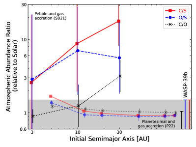
Figure 1: Predicted atmospheric ratios of C/S, O/S, and C/O based on initial planet location, from the planet formation models of Schneider & Bitsch (2021b, SB21; upper, thicker curves) and Pacetti et al. (2022, P22; lower, thinner curves). Although individual models span a range of final compositions (only the log-mean and standard deviation of each model set are plotted here), overall the differences suggest that volatile-to-sulfur ratios could provide a strong test as to whether a planet formed mainly via pebble or planetesimal accretion. The error bars at bottom-right and the shaded region show the abundance ratios inferred for WASP-39b from Fig. 4.

3 Modeling

3.1 Modeling Details

Having shown that volatile-to-sulfur abundances may test planet formation theories, we now explore how atmospheric S — as measured by SO₂ abundances — can reveal different atmospheric compositions. Many factors have a strong impact on a planet’s SO₂ abundance. E.g., SO₂ production is predicted to drop off steeply at $\lesssim$1000 K (Polman et al., 2023) and for FUV irradiation considerably higher than that experienced by WASP-39b (Tsai et al., 2023); and aerosol formation could also deplete elements that would otherwise end up in photochemical SO₂. Nonetheless, in this study we restrict our exploration to chemical composition and leave these other axes to future studies.

We examine a three-dimensional parameter space of atmospheric elemental abundances: $11^{3}$ combinations of a range of elemental enhancements of carbon, oxygen, and sulfur (from solar to 100$\times$ solar), using the VULCAN photochemical kinetics code (Tsai et al., 2017, 2021). For each combination of C, O, and S enhancement we calculate atmospheric abundance profiles using VULCAN’s SNCHO chemical network, which includes 575 chemical and photochemical reactions. We use WASP-39b as our simulated target; based on initial analyses of its spectrum, we hold all abundances other than C, O, and S to 10$\times$ solar (JTEC Team et al., 2023; Rustamkulov et al., 2023; Alderson et al., 2023; Ahrer et al., 2023; Feinstein et al., 2023; Tsai et al., 2023). The star WASP-39’s XUV flux remains largely unknown, so we adopt the same stellar spectrum used by Tsai et al. (2023). We compute our grid using two different, pre-determined temperature profiles, one each for the GCM-derived morning and evening terminator profiles presented by Tsai et al. (2023). These thermal profiles are broadly consistent with the single profile recently retrieved by Constantinou et al. (2023). Their retrieved, constant-with-altitude SO₂ abundances are broadly consistent with (if somewhat lower than) the detailed abundance profiles of Tsai et al. (2023) and of this work; further work is needed to compare abundances retrieved in this way with the predictions of photochemical codes. Finally, we also use the same $K_{zz}$ profile described by Tsai et al. (2023), scaling with pressure as $P^{-1/2}$ (following Lindzen, 1981; Moses et al., 2022). The system parameters and abundance values we used in our analysis are listed in Table 1. All the VULCAN outputs are available as machine-readable supplements to this paper.

Table 1: Model Parameters:

Name	Units	Description	Value	Source
System parameters:
$R_{*}$	$R_{\odot}$	Stellar radius	0.932	Carter & May, et al., in prep.
$R_{P}$	$R_{J}$	Planetary radius	1.279	Carter & May, et al., in prep.
$M_{P}$	$M_{J}$	Planetary mass	0.281	Carter & May, et al., in prep.
$g_{P}$	m s-2	Planetary surface gravity	4.26	Carter & May, et al., in prep.
$a$	AU	Semimajor axis	0.04828	Carter & May, et al., in prep.
Modeling parameters:
He/H	–	Solar volume mixing ratio	$8.38\times 10^{-2}$	Lodders (2020)
C/H	–	Solar volume mixing ratio	$2.95\times 10^{-4}$	Lodders (2020)
O/H	–	Solar volume mixing ratio	$5.37\times 10^{-4}$	Lodders (2020)
S/H	–	Solar volume mixing ratio	$1.41\times 10^{-5}$	Lodders (2020)
$P$	bar	Pressure range	10–10-9
$P_{0}$	bar	Reference pressure	0.01
$z$	deg	Zenith angle	83
C	–	Abundance relative to Solar	1, 1.8, 3, 5.6, 7.5, 10, 13, 18, 30, 56, 100
O	–	Abundance relative to Solar	1, 1.8, 3, 5.6, 7.5, 10, 13, 18, 30, 56, 100
S	–	Abundance relative to Solar	1, 1.8, 3, 5.6, 7.5, 10, 13, 18, 30, 56, 100

We then use the petitRadTrans radiative transfer code (Mollière et al., 2019) to calculate synthetic transmission spectra corresponding to each VULCAN run. We convert VULCAN’s volume mixing ratios (VMRs) to petitRadTrans’ mass mixing ratios. We use petitRadTrans’ medium-resolution, correlated-k opacity sources, giving our synthetic spectra a resolving power of $\sim$1,000 from 1–25 $\mu m$. The molecules and opacity sources we include are H₂O, CO, CO₂, SO₂, CH₄, HCN, H₂S, CH₃, C₂H₂, C₂H₄, CN, CH, OH, and SH (Rothman et al., 2010; Polyansky et al., 2018; Yurchenko et al., 2020; Underwood et al., 2016; Yurchenko & Tennyson, 2014; Harris et al., 2006; Barber et al., 2014; Chubb et al., 2018; Azzam et al., 2016; Adam et al., 2019; Chubb et al., 2020; Brooke et al., 2014; Bernath, 2020; Syme & McKemmish, 2020; Masseron et al., 2014; Brooke et al., 2016; Yousefi et al., 2018; Gorman et al., 2019). We have three sets of synthetic spectra: one each for the morning and evening thermal profiles, plus a set of spectra that are the mean of the morning and evening spectra (corresponding to the transmission spectrum that would be observed during transit). All the petitRadTrans synthetic spectra are also available as machine-readable supplements to this paper.

We note that the abundances of 15 elements (including C and O, but not S) were measured for WASP-39 (Polanski et al., 2022), revealing a composition for which every element is consistent with the solar values at $<1\sigma$. Similarly, the C/O ratio of $0.46\pm 0.09$ is consistent with the solar value of 0.55 (assuming the abundances of Lodders, 2020). Therefore, although generally stellar (not solar) abundances are the appropriate referent for atmospheric modeling, we elect to use abundance levels scaled from Solar values given WASP-39’s chemical similarity to the Sun (Polanski et al., 2022).

Finally, we also note that for a nominal WASP-39b model with an atmosphere enhanced to 10$\times$ Solar abundances, the transmission contribution function in regions of maximal SO₂ absorption span a pressure range of roughly 0.01–30 mbar. Although a weighted average of the SO₂ concentration (e.g., via weighting by atmospheric mass density) may give a somewhat more representative view of the peak of the photochemical SO₂ abundance, for simplicity (and to facilitate direct comparison with the work of Tsai et al., 2023) here we report the average of our modeled SO₂ concentration from 0.01–10 mbar.

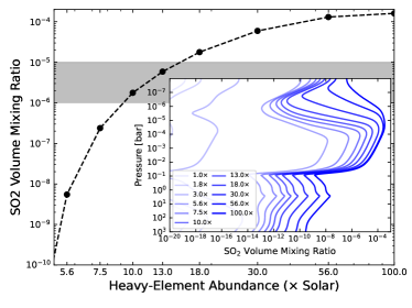
Figure 2: In the main panel, the dashed line shows the SO₂ VMR, averaged from 0.01–10 mbar, as all elemental abundances are increased in lockstep; the gray region shows the approximate SO₂ abundance reported for WASP-39b. The inset shows the full vertical SO₂ profiles.

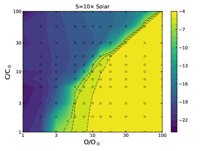
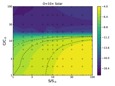
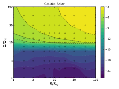
Figure 3: Abundance of SO₂ (averaged from 0.01–10 mbar) as combinations of two elemental abundances are varied: C vs. O (top), C vs. S (middle), and O vs. S (bottom). The points indicate the locations of the model grid points, which we linearly interpolate between. In each panel, all other elements are held fixed at 10$\times$ Solar abundance.

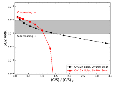
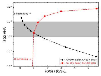
Figure 4: Abundance of SO₂ (averaged from 0.01–10 mbar) as the atmospheric ratios of C/O (top), C/S (middle), and O/S (bottom) are varied. The gray regions show the approximate SO₂ abundance reported for WASP-39b, which correspond here to C/S and O/S $\lesssim$1.5.

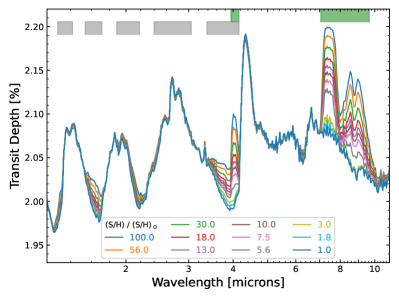
Figure 5: Synthetic spectra showing the effect of varying the S/H ratio from 1–100$\times$ Solar while keeping O/H and C/H at 10$\times$ Solar, as inferred for WASP-39b (equivalent to varying C/S and O/S from 10–0.1$\times$ Solar). At 10$\times$ Solar metallicity SO₂ is detectable up to volatile-to-sulfur ratios of $\lesssim$3$\times$ Solar. The shaded rectangles show where absorption is dominated by SO₂ (green) and by H₂S (grey).

3.2 Differences From Previous Studies

Our modeling effort expands on previous exploration of SO₂ in several ways. The first such study presented a comprehensive examination of SO₂ abundance in hot Jupiter atmospheres (Polman et al., 2023). Their study also used the VULCAN code to cover metallicities of 1–20$\times$ Solar, three values of $K_{zz}$ (constant with altitude, but spanning three orders of magnitude), C/O ratios from 0.25–0.9, several different stellar spectra, and three planetary temperatures (spanning 400 K). More recently, Tsai et al. (2023) demonstrated that SO₂ causes the 4.2 µm absorption feature seen in JWST spectroscopy of WASP-39b (Rustamkulov et al., 2023; Ahrer et al., 2023; Alderson et al., 2023). That investigation used four photochemistry codes (including VULCAN) to span three metallicities (from 5 to 20$\times$ Solar), three $K_{zz}$ profiles (spanning two orders of magnitude), three C/O ratios (from 0.25 to 0.75), three stellar spectra (spanning two orders of magnitude in irradiation), and a range of temperatures (from 600 to 2000 K).

Our analysis builds upon both these works by (i) examining a more densely sampled and fully two-dimensional grid of C and O abundances, (ii) adding a third dimension by exploring a wide range of S abundances, and (iii) extending the analysis up to significantly higher atmospheric metallicities.

3.3 Discussion and Interpretation

Fig. 2 shows how the SO₂ abundance increases as all three elements (C, O, and S) are increased in lockstep. Whereas the abundance of the triatomic CO₂ (produced via equilibrium chemical processes) increases quadratically with metallicity (Zahnle et al., 2009b), the more complicated formation pathways of SO₂ result in a more complicated metallicity dependence: much steeper than CO₂ at low metallicity, and shallower at high metallicity. This suggests that if high-metallicity ($>100\times$ Solar) ice giants also form photochemical SO₂, its VMR is unlikely to be $\gtrsim$200 ppm (as found by Tsai et al., 2021).

Fig. 3 shows three slices through our 3D abundance grid, depicting the SO₂ volume mixing ratio (VMR, averaged from 0.01–10 mbar) versus C, O, and S abundances. Fig. 4 shows 1D slices as plotted against the abundance ratios C/O, C/S, and O/S.

Fig. 4 reveals that the SO₂ abundances decreases as the atmospheric C/O ratio increases (while the S abundance is held constant). Consistent with the results of Polman et al. (2023), the dependence on C/O is similar regardless of whether we increase C or decrease O (though with a slightly steeper dependence when O is varied). In either case, when C/O increases beyond the Solar value the SO₂ abundance rapidly drops below detectable levels. The detection of SO₂ is therefore a strong sign of a C/O ratio $\lesssim$ the Solar value.

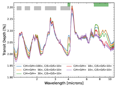
Figure 6: Synthetic spectra showing the effect of varying C/H and O/H from 10–100$\times$ Solar while keeping the C/S and O/S ratios at 10$\times$ Solar, as might be expected from pebble accretion (equivalent to varying S/H from 1–10$\times$ Solar). At 10$\times$ Solar C/S and O/S, SO₂ is detectable down to a volatile enhancement level of $\sim$18$\times$ Solar. The shaded rectangles show where absorption is dominated by SO₂ (green) and by H₂S (grey). Note that for volatile enrichment $\gtrsim$100$\times$ Solar the amplitude of spectral features begins to decrease as the mean molecular weight begins to increase.

More excitingly, Fig. 4 shows how measurements of the SO₂ abundance can distinguish between a variety of volatile-to-sulfur ratios. JWST transit spectroscopy of WASP-39b reveal it to have an atmospheric metallicity $\sim$10$\times$ Solar, a C/O ratio $\lesssim$ the Solar value, and a SO₂ VMR of 1–10 ppm (JTEC Team et al., 2023; Rustamkulov et al., 2023; Alderson et al., 2023; Ahrer et al., 2023; Feinstein et al., 2023; Tsai et al., 2023). Assuming an overall metallicity of 10$\times$ Solar, the bottom two panels of Fig. 4 show that the SO₂ measurement constrains both C/S and O/S to $\lesssim$1.5$\times$ Solar. Reference to Fig. 1 demonstrates that such values are rather more consistent with planetesimal accretion models (Turrini et al., 2021; Pacetti et al., 2022) than with pebble accretion (Schneider & Bitsch, 2021b). The only pebble formation models of Schneider & Bitsch (2021b) that can approximately reproduce these ratios assume an initial formation location of 3 AU and $\alpha\leq 5\times 10^{-4}$.

We also show a few representative examples of our synthetic transmission spectra. In Fig. 5 we see the effect on WASP-39b’s transmission spectra of varying the S/H ratio from 1–100$\times$ Solar, while keeping O/H=C/H=10$\times$ Solar (as inferred for WASP-39b); this is equivalent to varying C/S and O/S from 10$\times$ down to 0.1$\times$ Solar. The figure shows that at WASP-39b-like volatile enrichment levels, SO₂ has a significant impact on a planet’s transmission spectrum for S/H$\gtrsim 3\times$ Solar (C/S or O/S $\lesssim$3$\times$ Solar).

Lest one conclude from Figs. 4 and 5 that high volatile-to-sulfur ratios $\gtrsim$3$\times$ Solar are impossible to detect, Fig. 6 shows that SO₂ is easily discernible at C/S=O/S=10$\times$ Solar — so long as the atmospheric volatile enrichment (i.e., O/H and C/H) is $\gtrsim$18$\times$ Solar. Since smaller, lower-mass planets are thought to form with more metal-rich atmospheres (e.g., Fortney et al., 2013), such planets may therefore be the best targets to look for SO₂ to reveal the extreme volatile-to-sulfur ratios that would be a signpost of formation via pebble accretion.

4 Conclusions

4.1 Summary

In conclusion, we have shown that a planet’s formation and migration history may imprint unique elemental abundance signatures on the planet’s atmosphere: specifically, on the C/S and O/S ratios. In particular, Fig. 1 and Sec. 2 demonstrate how formation models in which solids are predominately accreted as pebbles often predict much higher volatile-to-sulfur ratios (C/S and O/S) than models in which solids are accreted as planetesimals. Although a planet’s N/S ratio has also been proposed as a diagnostic of formation (Turrini et al., 2021; Pacetti et al., 2022), detecting both these species in a gas giant may be challenging: S is mostly only visible as SO₂ at $T\gtrsim 1000$ K (Polman et al., 2023) while N is mostly detectable as NH₃ at $T\lesssim 1000$ K (Ohno & Fortney, 2022b). Thus the C/S and O/S ratios may be more generally useful (and measurable) than N/S.

We then present a grid of photochemical models and synthetic spectra for WASP-39b in which C, O, and S abundances are varied to determine the impact on the observable SO₂ signature (Sec. 3 and Fig. 3). Consistent with previous studies, we find that SO₂ should be most prevalent at high metallicity; we also find that it should be more abundance at higher elemental O and S abundances but lower C abundances. By examining how the SO₂ abundance varies with C/S and O/S in our models, Fig. 4 shows that WASP-39b’s atmospheric SO₂ abundance may constrain C/S and O/S to levels more consistent with planetesimal accretion than pebble accretion – although some pebble accretion models also predict lower volatile-to-sulfur ratios that seem more consistent with WASP-39b.

Additional work is certainly needed to confirm this conclusion. The main planet formation models discussed in Sec. 2 all result in planets more massive than WASP-39b, which suggests the need for caution in linking these models to WASP-39b’s composition. Also, relatively few planet formation studies report the final planetary C, O, and S abundances — additional, independent models tracking these abundances and featuring either planetesimal or pebble accretion would be extremely useful to understand the robustness of the dichotomy in volatile-to-sulfur ratios shown in Fig. 1.

4.2 Future Work

There is also considerable scope for further exploration of the planetary and stellar parameters that impact the observed SO₂ abundance. These include bolometric irradiation, received XUV flux, aerosols, additional T-P profiles, better high-temperature opacity data in the UV, and the observability of SO₂ or other S-bearing species via thermal emission — not to mention the impact of additional species such as nitrogen.

Regarding high-energy stellar flux, Hobbs et al. (2021) reported that increasing UV flux by up to two orders of magnitude merely results in the SO₂ abundance profile being pushed to somewhat deeper pressures, but with the overall abundance relatively unchanged. On the other hand, Tsai et al. (2023) instead find that increasing the NUV flux minimally changes the SO₂ profile, while increasing the FUV flux can decrease the SO₂ abundance by $\sim 10^{4}$. If the influence of UV flux could be pinned down, it would provide strong motivation for measuring the intrinsic spectra of stars with planets expected to exhibit SO₂ (or other) photochemistry.

Also regarding WASP-39’s intrinsic stellar spectrum, we note that [S/H] has still not been measured for this star. Although the star’s generally Solar-like elemental abundances (Polanski et al., 2022) suggest that its sulfur abundance may also be nearly Solar, [S/H] should be measured for WASP-39 as it has been for many other planet-hosting stars (e.g., Costa Silva et al., 2020) to confirm the expected, Solar-like sulfur abundance.

In this work we have not explored planetary nitrogen abundance, but it may also be an important axis. For example, the nitrogen-to-oxygen ratio in gas and solids should vary by several orders of magnitude from 1–100 AU (Ohno & Fortney, 2022a). And if planet formation is dominated by planetesimal accretion, then the sulfur-to-nitrogen ratio may be a useful probe of whether a gas giant accreted most of its mass via solids or gas (Turrini et al., 2021).

Further exploration is also warranted into the effect of different $K_{zz}$ values on the observable SO₂ abundance. Tsai et al. (2023) found that varying their $K_{zz}$ profile (nominally spanning $5\times 10^{7}$ to $10^{11}\mathrm{~{}cm}^{2}\mathrm{\ s}^{-1}$) by $\pm$ an order of magnitude had only a minor impact, consistent with the results of Hobbs et al. (2021) from isothermal models with $K_{zz}$ spanning $10^{6}$–$10^{12}\mathrm{~{}cm}^{2}\mathrm{\ s}^{-1}$. In contrast, other studies report that increasing a constant-with-altitude $K_{zz}$ to $10^{11}\mathrm{~{}cm}^{2}\mathrm{\ s}^{-1}$ sharply decreases the amount of observable SO₂ (Tsai et al., 2021; Polman et al., 2023). Although $K_{zz}$ is a challenging quantity to empirically constrain, it would at least be useful to understand how it quantitatively impacts the measurement of SO₂ in planetary atmospheres.

Future studies might also test the impact of self-consistently modeling the thermal and chemical profiles in the atmospheres, thereby accounting for thermal back-reaction of photochemical species such as SO₂ on the planet’s vertical temperature structure. Similarly, the interplay of global circulation and atmospheric chemistry may reveal that predictions made from 1D models (as in this work) – or even from post-processed chemistry-free global circulation models – may lead to inaccurate interpretations of exoplanet measurements (Lee et al., 2023).

JWST/NIRSpec may be the ideal instrument to best constrain C, O, and S and so begin to test the connection between atmospheric SO₂ and planet formation posited in this paper. Even the G395 modes (let alone the Prism!) cover multiple strong bands of CO₂, CO, CH₄, and H₂O, as well as the SO₂ described by Tsai et al. (2023). The signal of SO₂ may be even stronger in the MIRI/LRS bandpass, but the overall S/N may be lower there – in addition, shorter wavelength coverage may still be needed to provide a complete elemental assay; the feasibility of MIRI for SO₂ measurements is currently under study by multiple groups.

Finally, although SO₂ is not always the dominate sulfur carrier in H₂-dominated exoplanet atmospheres, the H₂S that carries most of the sulfur is much more difficult to detect and quantify (Polman et al., 2023). Furthermore, since the vertical abundance profile of photochemical SO₂ varies significantly with altitude (Fig. 2), retrievals in which the abundance is assumed to be constant with altitude may somewhat underestimate the true SO₂ abundance (which might already affect the retrieval results of Constantinou et al., 2023). For all these reasons, physically-motivated photochemical models of SO₂in H₂-dominated exoplanets should therefore remain a key tool to unraveling the atmospheric properties of such planets.

References

- Adam et al. (2019) Adam, A. Y., Yachmenev, A., Yurchenko, S. N., & Jensen, P. 2019, Journal of Physical Chemistry A, 123, 4755
- Ahrer et al. (2023) Ahrer, E.-M., Stevenson, K. B., Mansfield, M., et al. 2023, Nature, 614, 653
- Alderson et al. (2023) Alderson, L., Wakeford, H. R., Alam, M. K., et al. 2023, Nature, 614, 664
- Asplund et al. (2009) Asplund, M., Grevesse, N., Sauval, A. J., & Scott, P. 2009, ARA&A, 47, 481
- Azzam et al. (2016) Azzam, A. A. A., Tennyson, J., Yurchenko, S. N., & Naumenko, O. V. 2016, MNRAS, 460, 4063
- Barber et al. (2014) Barber, R. J., Strange, J. K., Hill, C., et al. 2014, MNRAS, 437, 1828
- Batalha et al. (2017) Batalha, N., Bean, J. L., Stevenson, K. B., et al. 2017, The Transiting Exoplanet Community Early Release Science Program, JWST Proposal ID 1366. Cycle 0 Early Release Science
- Bernath (2020) Bernath, P. F. 2020, J. Quant. Spec. Radiat. Transf., 240, 106687
- Biazzo et al. (2022) Biazzo, K., D’Orazi, V., Desidera, S., et al. 2022, A&A, 664, A161
- Bitsch et al. (2022) Bitsch, B., Schneider, A. D., & Kreidberg, L. 2022, A&A, 665, A138
- Brooke et al. (2016) Brooke, J. S., Bernath, P. F., Western, C. M., et al. 2016, Journal of Quantitative Spectroscopy and Radiative Transfer, 168, 142
- Brooke et al. (2014) Brooke, J. S. A., Ram, R. S., Western, C. M., et al. 2014, ApJS, 210, 23
- Chubb et al. (2020) Chubb, K. L., Tennyson, J., & Yurchenko, S. N. 2020, MNRAS, 493, 1531
- Chubb et al. (2018) Chubb, K. L., Naumenko, O., Keely, S., et al. 2018, J. Quant. Spec. Radiat. Transf., 218, 178
- Constantinou et al. (2023) Constantinou, S., Madhusudhan, N., & Gandhi, S. 2023, ApJ, 943, L10
- Costa Silva et al. (2020) Costa Silva, A. R., Delgado Mena, E., & Tsantaki, M. 2020, A&A, 634, A136
- Feinstein et al. (2023) Feinstein, A. D., Radica, M., Welbanks, L., et al. 2023, Nature, 614, 670
- Fortney et al. (2013) Fortney, J. J., Mordasini, C., Nettelmann, N., et al. 2013, ApJ, 775, 80
- Gorman et al. (2019) Gorman, M. N., Yurchenko, S. N., & Tennyson, J. 2019, MNRAS, 490, 1652
- Harris et al. (2006) Harris, G. J., Tennyson, J., Kaminsky, B. M., Pavlenko, Y. V., & Jones, H. R. A. 2006, MNRAS, 367, 400
- Heng et al. (2016) Heng, K., Lyons, J. R., & Tsai, S.-M. 2016, ApJ, 816, 96
- Hobbs et al. (2021) Hobbs, R., Rimmer, P. B., Shorttle, O., & Madhusudhan, N. 2021, MNRAS, 506, 3186
- JTEC Team et al. (2023) JTEC Team, Ahrer, E.-M., Alderson, L., et al. 2023, Nature, 614, 649
- Kama et al. (2019) Kama, M., Shorttle, O., Jermyn, A. S., et al. 2019, ApJ, 885, 114
- Le Gal et al. (2021) Le Gal, R., Öberg, K. I., Teague, R., et al. 2021, ApJS, 257, 12
- Lee et al. (2023) Lee, E. K. H., Tsai, S.-M., Hammond, M., & Tan, X. 2023, arXiv e-prints, arXiv:2302.09525
- Lindzen (1981) Lindzen, R. S. 1981, J. Geophys. Res., 86, 9707
- Lodders (2003) Lodders, K. 2003, ApJ, 591, 1220
- Lodders (2020) —. 2020, Oxford Research Enc. of Pl. Sci., arXiv:1912.00844
- Lothringer et al. (2021) Lothringer, J. D., Rustamkulov, Z., Sing, D. K., et al. 2021, ApJ, 914, 12
- Madhusudhan (2012) Madhusudhan, N. 2012, ApJ, 758, 36
- Masseron et al. (2014) Masseron, T., Plez, B., Van Eck, S., et al. 2014, A&A, 571, A47
- Mollière et al. (2019) Mollière, P., Wardenier, J. P., van Boekel, R., et al. 2019, A&A, 627, A67
- Mordasini et al. (2016) Mordasini, C., van Boekel, R., Mollière, P., Henning, T., & Benneke, B. 2016, ApJ, 832, 41
- Moses et al. (2022) Moses, J. I., Tremblin, P., Venot, O., & Miguel, Y. 2022, Experimental Astronomy, 53, 279
- Öberg et al. (2011) Öberg, K. I., Murray-Clay, R., & Bergin, E. A. 2011, ApJ, 743, L16
- Ohno & Fortney (2022a) Ohno, K., & Fortney, J. J. 2022a, arXiv e-prints, arXiv:2211.16876
- Ohno & Fortney (2022b) —. 2022b, arXiv e-prints, arXiv:2211.16877
- Oka et al. (2011) Oka, A., Nakamoto, T., & Ida, S. 2011, ApJ, 738, 141
- Pacetti et al. (2022) Pacetti, E., Turrini, D., Schisano, E., et al. 2022, ApJ, 937, 36
- Polanski et al. (2022) Polanski, A. S., Crossfield, I. J. M., Howard, A. W., Isaacson, H., & Rice, M. 2022, Research Notes of the American Astronomical Society, 6, 155
- Polman et al. (2023) Polman, J., Waters, L. B. F. M., Min, M., Miguel, Y., & Khorshid, N. 2023, A&A, 670, A161
- Polyansky et al. (2018) Polyansky, O. L., Kyuberis, A. A., Zobov, N. F., et al. 2018, MNRAS, 480, 2597
- Rivière-Marichalar et al. (2022) Rivière-Marichalar, P., Fuente, A., Esplugues, G., et al. 2022, A&A, 665, A61
- Rothman et al. (2010) Rothman, L., Gordon, I., Barber, R., et al. 2010, JQSRT, 111, 2139
- Rustamkulov et al. (2023) Rustamkulov, Z., Sing, D. K., Mukherjee, S., et al. 2023, Nature, 614, 659
- Schneider & Bitsch (2021a) Schneider, A. D., & Bitsch, B. 2021a, A&A, 654, A71
- Schneider & Bitsch (2021b) —. 2021b, A&A, 654, A72
- Schneider & Bitsch (2022) —. 2022, How drifting and evaporating pebbles shape giant planets (Corrigendum), Astronomy & Astrophysics, Volume 659, id.C3, 3 pp., doi:10.1051/0004-6361/202141096e
- Seager et al. (2005) Seager, S., Richardson, L. J., Hansen, B. M. S., et al. 2005, ApJ, 632, 1122
- Syme & McKemmish (2020) Syme, A.-M., & McKemmish, L. K. 2020, MNRAS, 499, 25
- Tsai et al. (2017) Tsai, S.-M., Lyons, J. R., Grosheintz, L., et al. 2017, ApJS, 228, 20
- Tsai et al. (2021) Tsai, S.-M., Malik, M., Kitzmann, D., et al. 2021, ApJ, 923, 264
- Tsai et al. (2023) Tsai, S.-M., Lee, E. K. H., Powell, D., et al. 2023, arXiv e-prints, arXiv:2211.10490
- Turrini et al. (2021) Turrini, D., Schisano, E., Fonte, S., et al. 2021, ApJ, 909, 40
- Underwood et al. (2016) Underwood, D. S., Tennyson, J., Yurchenko, S. N., et al. 2016, Monthly Notices of the Royal Astronomical Society, 459, 3890
- Wood et al. (2019) Wood, B. J., Smythe, D. J., & Harrison, T. 2019, American Mineralogist, 104, 844
- Yousefi et al. (2018) Yousefi, M., Bernath, P. F., Hodges, J., & Masseron, T. 2018, Journal of Quantitative Spectroscopy and Radiative Transfer, 217, 416
- Yurchenko et al. (2020) Yurchenko, S. N., Mellor, T. M., Freedman, R. S., & Tennyson, J. 2020, MNRAS, 496, 5282
- Yurchenko & Tennyson (2014) Yurchenko, S. N., & Tennyson, J. 2014, MNRAS, 440, 1649
- Zahnle et al. (2009a) Zahnle, K., Marley, M. S., & Fortney, J. J. 2009a, ArXiv e-prints, arXiv:0911.0728
- Zahnle et al. (2009b) Zahnle, K., Marley, M. S., Freedman, R. S., Lodders, K., & Fortney, J. J. 2009b, ApJ, 701, L20
- Zahnle et al. (2016) Zahnle, K., Marley, M. S., Morley, C. V., & Moses, J. I. 2016, ApJ, 824, 137