Exploring Thousands of Nearby Hierarchical Systems with Gaia and Speckle Interferometry

Abstract

There should be about 10,000 stellar hierarchical systems within 100 pc with primary stars more massive than 0.5 $M_{\odot}$ , and a similar amount of less massive hierarchies. A list of 8000 candidate multiples is derived from wide binaries found in the Gaia Catalog of Nearby Stars where one or both components have excessive astrometric noise or other indicators of inner subsystems. A subset of 1243 southern candidates were observed with high angular resolution at the 4.1 m telescope, and 503 new pairs with separations from 0$\farcs$03 to 1″ were resolved. These data allow estimation of the inner mass ratios and periods and help to quantify the ability of Gaia to detect close pairs. Another 621 hierarchies with known inner periods come from the Gaia catalog of astrometric and spectroscopic orbits. These two non-overlapping groups, combined with existing ground-based data, bring the total number of known nearby hierarchies to 2754, reaching a completeness of $\sim$22% for stars above 0.5 $M_{\odot}$ . Distributions of their periods and mass ratios are briefly discussed, and the prospects of further observations are outlined.

1 Introduction

Stars form in groups. Almost every star has been gravitationally bound to some other star or stars in their infancy (Lee et al., 2019), and a substantial fraction of these systems have survived, as evidenced by the multiplicity statistics of mature field populations (Moe & Di Stefano, 2017; Offner et al., 2022). Statistics of stellar systems helps us to understand their formation and early evolution. Hierarchical systems are particularly informative in this regard. However, owing to the vast range of parameters (separations, mass ratios), the complete view of even the nearest population of stellar hierarchies has been difficult to grasp. The relatively well studied sample of solar-type stars within 25 pc contains only 56 hierarchical systems (Raghavan et al., 2010).

The Gaia astrometric space mission (Gaia Collaboration et al., 2016, 2021a) has dramatically changed the landscape of Galactic astronomy in many ways. The mission continues, and the use of its intermediate data for the study of stellar systems is a rapidly growing field (e.g. El-Badry et al., 2021; Tokovinin, 2022a). The Gaia Catalog of Nearby Stars (GCNS) within 100 pc (Gaia Collaboration et al., 2021b), based on the Gaia Early Data Release 3 (eDR3), gives a complete census of all stars down to the hydrogen burning limit (except for some binaries lacking parallaxes). Owing to its exquisite astrometric precision, Gaia can detect a substantial fraction of binary systems in the 100 pc volume. However, the periods and mass ratios of most candidate close binaries remain essentially unconstrained. The Non-Single Star (NSS) catalog (Gaia Collaboration et al., 2022; Pourbaix et al., 2022), part of the Gaia data release 3 (DR3), contains orbital elements only for a small fraction of astrometric and spectroscopic binaries detected by Gaia.

In this work, I open the treasure trove of Gaia data to get a better view of nearby stellar hierarchies. A candidate list is created by isolating bound pairs of stars found in the GCNS and looking at those that contain signs of inner subsystems according to the Gaia binarity indicators. Naturally, some of these hierarchies are already known from prior work. A subset of the new candidates have been observed systematically by speckle interferometry at the 4.1 m Southern Astrophysical Research Telescope (SOAR) in 2021–2023, and these results are reported here. About half of the candidates were resolved, providing estimates of their mass ratios and likely periods. At the same time, these resolutions allow better understanding of the discovery potential of the Gaia binarity indicators. Complementing the known hierarchies by these new systems and by the systems with inner orbits determined by Gaia leads to a sample of 2758 main-sequence hierarchies within 100 pc with known or estimated inner and outer periods. Their primary stars are generally more massive than $\sim$0.7 $M_{\odot}$ . A glimpse of their statistics (still incomplete but much better than in the pre-Gaia era) is given, and directions of future research are outlined.

2 Gaia Hierarchies within 100 pc

2.1 Number of Hierarchies within 100 pc

The GCNS (Gaia Collaboration et al., 2021b) is a rich source of hierarchical systems in a volume-limited sample, with the potential to make a major contribution to their statistics. It contains 331,312 entries. However, the GCNS misses close binaries with components of comparable brightness that do not have parallaxes in eDR3. The fraction of missing stars was estimated at 7.4% in the GCNS, based on its data for 10 pc volume. The peak of binary separation distribution at $\sim$50 au corresponds to an angular separation of 0$\farcs$5 at 100 pc, so the bias against binaries in the complete GCNS could be larger than in its 10 pc portion. Empirical characterization of the Gaia bias against binaries based on the new SOAR observations is provided below.

Figure 1: Estimated number of hierarchical systems within 100 pc in 0.1 $M_{\odot}$ mass bins.

The distribution of absolute magnitudes in the GCNS peaks at $M_{G}=10.5$ mag, reaching a density of 0.01 star pc^-3 mag^-1, and drops smoothly on both sides of the maximum (see Figure 16 in GCNS). The corresponding median mass is 0.32 $M_{\odot}$ according to the PARSEC isochrone for solar metallicity (Bressan et al., 2012). Let us estimate how many hierarchical (e.g. triple and higher-order) systems are there within 100 pc. It is well known that the fraction of hierarchies increases with mass, while the density of stars declines. I approximated the fraction of hierarchies vs. mass in Figure 1 of Offner et al. (2022) by a parabola $f_{H}\approx 0.146+0.255x+0.414x^{2}$, where $x=\log_{10}M/$$M_{\odot}$ , and multiplied the star counts in GCNS by this fraction (the masses are estimated from the absolute magnitudes $M_{G}$). The result in Figure 1 suggests a total number around 19,000 for masses above 0.2 $M_{\odot}$ (10,400 above 0.5 $M_{\odot}$ and 6,400 above 0.7 $M_{\odot}$ ). Additional 4,400 hierarchies are predicted in the first 0.1–0.2 $M_{\odot}$ bin, although $f_{H}$ for low-mass stars is poorly known. This model yields 4,062 hierarchies with masses from 0.8 to 1.25 $M_{\odot}$ within 100 pc, roughly matching 56 systems found in the 64$\times$ smaller volume by Raghavan et al. (2010).

2.2 Selection of Candidate Hierarchies

The GCNS provides a list of 19,176 pairs of stars, 16,556 of which are estimated to be bound. However, inner subsystems in triples bias Gaia measurements of parallaxes and proper motions (PMs), so many wide pairs with subsystems appear as unbound or even unrelated. To avoid potential bias against triples, I use the weaker criteria for selecting outer pairs, as outlined in Tokovinin (2022a):

• Parallaxes equal within 1 mas.

• Projected separation $s<20$ kau.

• Relative projected speed (in km s^-1 ) $\Delta V<10(10^{3}/s)^{0.5}$, where $s$ is expressed in au. This is a relaxed form of the boundness criterion which rejects optical companions but preserves the hierarchies. A similar approach was adopted by Hwang et al. (2020).

A search over GCNS with these criteria returns 24,604 systems, each containing from 2 to 5 stars (50,243 stars in total). Most systems are just wide binaries, except 944 triples, 42 quadruples, and one quintuple, $\xi$ Sco. The relaxed criteria give a larger sample of wide systems compared to the list of binaries given in the GCNS. The median mass of stars in our wide pairs is 0.44 $M_{\odot}$ (0.60 and 0.31 $M_{\odot}$ for the primary and secondary components, respectively). This is larger than the median mass in GCNS because binaries prefer stars more massive than average (in other words, the binary fraction increases with mass). Other catalogs of wide binaries based on Gaia have been published by Hartman & Lépine (2020); El-Badry et al. (2021); Zavada & Píška (2022), and others using a variety of approaches and selection criteria.

Each Gaia (and GCNS) entry contains two powerful diagnostics of unresolved binaries, namely the reduced unit weight error (RUWE) and the fraction of double transits, FDBL (IPDfmp in the Gaia terminology). I also explored another parameter, IPDgofha (an asymmetry parameter in the Gaia image analysis), but found it to be poorly correlated with RUWE and FDBL; for this reason, probably, the GCNS does not contain this parameter. So, FDBL, RUWE, and the variability of radial velocity (RVERR) are the main indicators of close binaries. Photometric variability caused by eclipses is yet another indicator, used in some studies of hierarchies (e.g. Hwang et al., 2020; Fezenko et al., 2022) but not relevant for this work.

It is generally assumed that RUWE$>$1.4 indicates significant deviations from a single-star astrometric solution, suggesting an unresolved binary (Belokurov et al., 2020; Penoyre et al., 2022). However, a large RUWE can be caused either by the genuine motion of the photocenter (i.e. an astrometric binary) or by the influence of a faint visual companion that spoils the Gaia astrometry by its presence; both situations occur and can be illustrated by concrete examples.

Figure 2: Top: fraction of double transits FDBL in the primary component of resolved Gaia binaries vs. their separation $\rho$ in arcseconds. The line is FDBL=100*(2.5 - $\rho$)/1.5. Bottom: RUWE of the primary component vs. $\rho$.

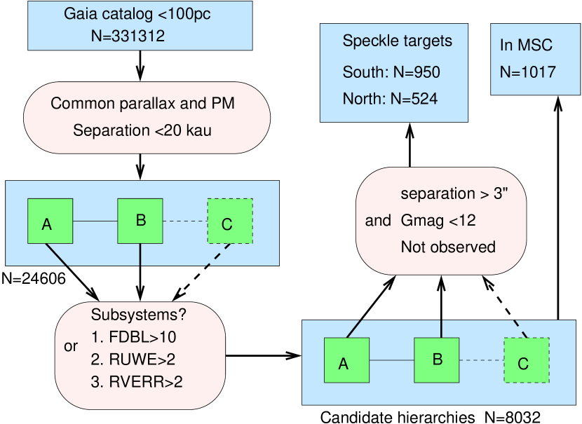
Figure 3: Block diagram showing selection of candidates for speckle observations.

The FDBL parameter, ranging from 0 to 100, is an even more powerful diagnostic of a close companion than RUWE; so far, it has received little attention in the literature. However, double transits do not always pinpoint inner subsystems. In a binary of $\sim$1″ separation, normally resolved by Gaia as two sources, double transits occur when the Gaia scans are nearly parallel to the binary. A plot of FDBL vs. binary separation $\rho$ in Figure 2 clearly shows an elevated FDBL for close pairs. An empirical condition FDBL$>100(2.5-\rho)/1.5$ inferred from this plot separates binaries with genuine subsystems from simple binaries with $\rho<2\farcs 5$. For the secondaries, a more strict criterion FDBL$>100(3.5-\rho)/1.5$ is adopted, based on a similar plot. However, as shown in the lower panel of Figure 2, many binaries closer than 2$\farcs$5 also have an elevated RUWE in their primary components, presumably caused by the disturbing influence of companions on the astrometric measurements. A plot of RUWE vs. the estimated speed of orbital motion, not shown here, reveals no correlation, so the non-linear orbital motion in these binaries is unlikely to be the cause of an elevated RUWE.

Figure 3 illustrates the process of selecting candidate hierarchies from the GCNS. About 1000 systems containing three (or more) related GCNS stars are obvious candidates; their subset has been studied in (Tokovinin, 2022a). Additional candidates are selected among wide binaries where the presence of an inner subsystem is inferred from the Gaia binarity flags: FDBL$>10$ (with a higher threshold for close outer pairs as noted above) or RUWE$>$2 or RVERR$>$2 km s^-1 . Application of these subjective criteria, adopted to maximize the reality of subsystems, leads to a pool of 8032 candidate hierarchies. In most cases, the parameters of the inner subsystems (periods and mass ratios) are unknown, so this sample by itself is not very informative for the statistics. For this reason some candidates were observed at SOAR, as reported below.

The list of 24,606 systems (including 8032 candidate hierarchies) is not provided here because, given the criteria, it can be derived from the original GCNS. The criteria for selecting binaries and subsystems were chosen subjectively, and modified criteria would result in a different list. The raw list has little value, as it serves only as a starting point for follow-up observations and for additional mining of the Gaia data.

The Multiple Star Catalog (MSC; Tokovinin, 2018a), holds a record of known hierarchies based on the literature. This is an eclectic data collection, heavily burdened by selection effects. On the other hand, the Washington Double Star Catalog (WDS; Mason et al., 2001), holds a similarly disparate collection of resolved (traditionally called “visual”) pairs, some of which are mere chance projections (optical pairs). The Gaia candidate hierarchies were matched to the WDS, and cases where the inner pairs in the Gaia candidates were actually resolved according to the WDS were singled out. Most of those triples were already present in the MSC, and 150 new ones where Gaia discovered distant tertiary components to the previously known visual binaries were added. With this increment, the MSC contained 1017 hierarchies within 100 pc. The work reported below has doubled this number. However, the completeness is still very poor in comparison with the expected number of hierarchies in Figure 1.

About 370 hierarchical systems within 100 pc documented in the MSC are not present in our candidate list. The most frequent classes are tight hierarchies with one or zero associated Gaia sources, and hierarchies where one component is a visual binary without Gaia astrometry. In a small number of cases, Gaia parallaxes are available for both components but are strongly biased by the subsystems, so that the two GCNS stars appear unrelated. For example, the primary star in 01579$-$2851 has a parallax of 12.45 mas in DR3, and 11.24 mas after fitting its astrometric orbit in the NSS; the latter coincides with the parallax of the secondary component. Obviously, this pair is missing from the list of candidates, which imposes a maximum parallax difference of 1 mas. A few hierarchies in the MSC have outer separations exceeding the adopted limit of 20 kau.

2.3 Data Organization

Information on binary and multiple stars in various databases is often affected by confusion. Such attributes as position, parallax, photometry, etc. may refer either to the blended light of several stars or to the individual stars. The term component is used here for referring to the data on astrometry and photometry of components of multiple systems, admitting that each component may host several stars and that the term resolved is fuzzy. The notion of component evolves with time as observing techniques improve. Gaia provides, for the first time, resolved photometry and astrometry of the individual components of many visual binaries wider than $\sim$1″. At the same time, the 2MASS photometry and position may still refer to the binary as a whole (a blend) because of the lower 2MASS resolution. For example, HIP 12548 is a single source in Gaia, although it contains four stars (Tokovinin, 2022b). In future Gaia data releases it may be split in two components separated by 0$\farcs$4, each component hosting a close pair.

A consistent identification scheme is implemented in the MSC (Tokovinin, 2018a). Each multiple system has a common 10-character MSC code based on the J2000 coordinates of its primary component. Components are designated by letters, their accurate coordinates for the J2000 epoch and other optional identifiers (e.g. in the HD or 2MASS catalogs) are provided. Subsystems are unions of components joined by a comma. In contrast, the WDS catalog of double stars (Mason et al., 2001) designates systems, rather than components. It uses the WDS codes (10-character strings based on the J2000 positions), but they may differ from the similar MSC codes either because a different star was taken as the primary or because the WDS codes are based on inaccurate positions (e.g. for many Luyten’s wide pairs).

In this work, the components of multiple systems that coincide with individual Gaia sources are designated by capital letters (with a few exceptions). The Gaia own identifiers are not used because they are not stable, changing between data releases. Instead, accurate positions (for J2000 or J2016 epochs) serve to match with Gaia and with other databases. If component B was resolved into a close pair, its members become Ba and Bb, while B refers to the blended Gaia source. Each system has a unique 10-character MSC code. This scheme minimizes confusion and provides a direct link to the MSC.

3 The SOAR Speckle Survey

3.1 Instrument, Observations, and Data Reduction

The high-resolution camera, HRCam, is an optical speckle imager operating at SOAR since 2007 (Tokovinin & Cantarutti, 2008). Over time, the instrument got a better detector, the observing procedure has been optimized, and the pipeline for data processing and calibration has been developed and tuned, converting HRCam into a high-efficiency survey facility with a typical yield of 300 stars per night (Tokovinin, 2018b). A survey of binary M-type dwarfs (Vrijmoet et al., 2022) and imaging of TESS exoplanet candidates (Ziegler et al., 2021) demonstrate the power of HRCam in this respect. The latest series of binary-star measurements and an overview of the ongoing HRCam observing programs are published in Tokovinin et al. (2022).

Observations of candidate hierarchies from the GCNS were conducted since 2021 October as a filler among other observing programs, using also some engineering time. As indicated in Figure 3, speckle targets were selected from the pool of 8032 candidates using additional criteria, namely $G>12$ mag (fainter stars require excellent seeing conditions), and $\rho>3\arcsec$ (to avoid potentially false candidates caused by wide companions). Only the RUWE and FDBL flags were considered, and only previously unobserved stars with a decl. south of $+20\arcdeg$  were placed on the SOAR program, resulting in 950 targets. A complementary list of 524 northern targets was produced. No speckle instruments in the Northern Hemisphere matching HRCam in productivity are available to make the northern extension of this survey a practical undertaking: it would require $\sim$10 nights at a 4 m telescope.

The main survey started in 2022 January. It was preceded by trial observations of candidate hierarchies selected by various criteria. In the last months of 2022, the observing program has been extended by adding candidate pairs with separations from 1″ to 3″. All results are reported here jointly. The $G<12$ mag limit corresponds to $M>0.7$$M_{\odot}$ at 100 pc. The median mass of the observed stars is 0.82 $M_{\odot}$ , and 80% are comprised between 0.60 and 1.23 $M_{\odot}$ . The median mass of the resolved stars (estimated in the same manner from their combined absolute magnitude) is 0.80 $M_{\odot}$ , and 80% are between 0.59 and 1.13 $M_{\odot}$ . Thus, the resolved speckle targets are, on average, slightly fainter than the unresolved ones. The likely explanation of this difference is a better prior coverage of bright stars (previously resolved pairs were not placed on the program).

In each HRCam observation, two image cubes of 200$\times$200 pixels and 400 frames are taken with an exposure time of 25 ms (8 s per cube) and a pixel scale of 15 mas. The observations were made in the $I$ filter (824/170nm) to maximize the flux from red stars and the detectability of faint red companions. The classical resolution limit set by diffraction is 40 mas, but closer pairs of near-equal stars were detected down to 30 mas separation from the asymmetry of the speckle power spectrum; measurements of their positions are inaccurate. Some close pairs were reobserved to confirm the detections and to follow their expected fast orbital motion. The approximate detection limits (resolution and maximum magnitude difference vs. separation) are determined by the speckle pipeline for each observation. They depend on the seeing conditions and on the target brightness. The contrast limit at 0$\farcs$15 separation, $\Delta I_{0.15}$, is increased here by 0.5 mag with respect to the original conservative estimates delivered by the pipeline to reflect better parameters of the resolved pairs. The astrometric calibration is common to all HRCam programs.

Table 1: Results of the SOAR Speckle Survey (fragment)

MSC	Comp.	R.A.	Dec.	Date	$\theta$	$\rho$	$\Delta I$	Flag	$\rho_{\rm min}$	$\Delta I_{0.15}$	$\Delta I_{1}$	NSS	System
(J2000)		(deg)	(deg)	(JY-2000)	(deg)	(′′)	(mag)		(′′)	(mag)	(mag)
00025$+$0440	AC	0.613899	4.668529	21.8909	196.7	1.0596	0.2	*	0.052	2.44	3.98	—	AC
00026$-$2814	A	0.661087	$-$28.236648	22.4418	0.0	0.0000	0.0	…	0.057	2.24	3.37	AORB	UR
00042$-$1008	A	1.051757	$-$10.141044	22.4419	0.0	0.0000	0.0	…	0.044	2.44	4.40	—	UR
00049$-$1811	A	1.237158	$-$18.178732	22.4419	0.0	0.0000	0.0	…	0.043	2.32	4.46	—	UR
00092$-$0408	A	2.306404	$-$4.133919	21.7542	351.5	0.0889	0.3	q	0.051	2.10	3.79	—	KPP2684Aa,Ab
00092$-$0408	A	2.306404	$-$4.133919	22.4446	0.0	0.0000	0.0	…	0.050	2.70	3.71	—	KPP2684Aa,Ab
00092$-$0408	A	2.306404	$-$4.133919	22.6823	0.0	0.0000	0.0	…	0.053	2.74	3.73	—	KPP2684Aa,Ab
00100$-$5358	A	2.491435	$-$53.958769	22.4447	0.0	0.0000	0.0	…	0.046	2.94	4.35	ASB1	UR
00111$-$0008	B	2.725629	$-$0.111976	22.4447	305.8	0.3546	2.5	q	0.051	2.65	3.81	—	Ba,Bb
00119$-$3533	A	2.962362	$-$35.546968	22.8452	125.4	0.0974	1.9	q	0.043	2.72	3.47	—	Aa,Ab
00119$-$3533	A	2.962362	$-$35.546968	23.0062	126.0	0.0963	1.9	q	0.041	3.07	5.76	—	Aa,Ab

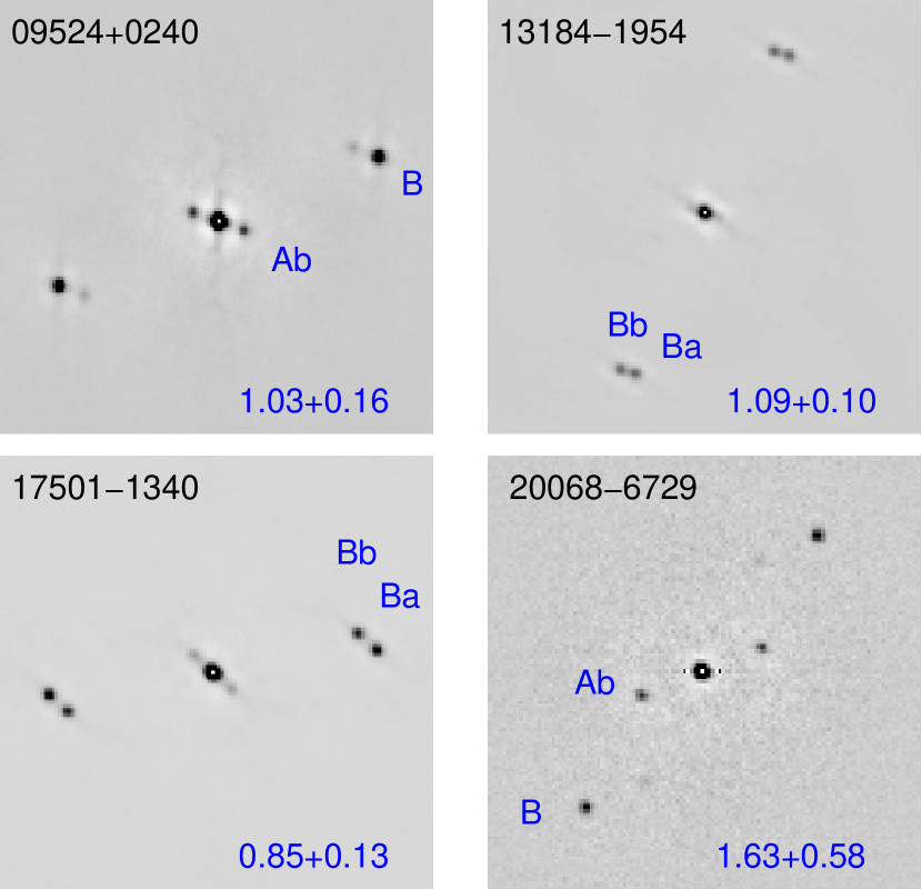
Figure 4: New triple stars where the wide companions are present in Gaia DR3 and the inner subsystems are resolved by SOAR. The speckle ACFs are displayed with an arbitrary negative stretch to highlight the companions. Each panel has an MSC label. The peaks corresponding to the companions are marked, and the outer and inner separations in arcseconds are indicated.

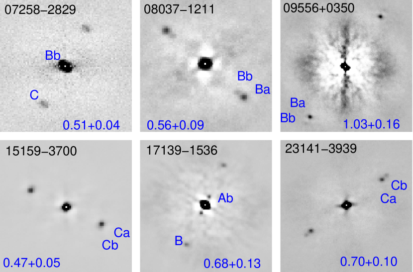
Figure 5: New compact triplets discovered by the SOAR speckle imaging of Gaia candidates. See the caption to Figure 4.

3.2 Results

Table 1, published fully electronically, presents the results of this survey. Its first columns contain the MSC code of the system (similar to the WDS code, but not always coincident), the component’s identifier, and its accurate equatorial coordinates for the J2000 epoch from the GCNS. This information should uniquely identify each observed target. When the measurement involves two Gaia sources, the component identifier has two characters. The following columns contain Julian year of the observation, position angle $\theta$, separation $\rho$, and magnitude difference $\Delta I$; for unresolved targets all these numbers are zero. Note that 00092$-$0408 A has been resolved in 2021.75 at 0$\farcs$089, but unresolved on two occasions in 2022. An optional flag after $\Delta I$ indicates cases where the magnitude difference is determined from the average image of a wide pair (*), when the quadrant is defined without 180° ambiguity (q), the data are noisy or below the diffraction limit (:), and a few observations of close pairs in the Strömgren $y$ band (y). The three following columns contain the detection limits: the minimum separation $\rho_{\rm min}$, and the maximum magnitude differences at 0$\farcs$15 and 1″ separations, $\Delta I_{0.15}$ and $\Delta I_{1}$, respectively. The next column gives a code of the NSS solution, if present (see Section 4) or — otherwise. The last column contains the WDS discoverer codes of the systems where appropriate (e.g. KPP2684Aa,Ab for the resolved primary star of the 3$\farcs$6 Gaia pair named KPP2684 in the WDS), otherwise designations like Ba,Bb for the newly resolved pairs, UR for unresolved sources, AB for Gaia pairs, or Aa,Ab and Aa,B for resolved triples.

Table 1 contains 1384 entries corresponding to 1243 unique targets (either single components or pairs); 1058 of them have single-letter component identifiers, 503 of which (48%) are resolved. There are 47 observed targets fainter than $G=12$ mag, eight of those are fainter than $G=14$ mag, and the faintest one has $G=17.3$ mag. Faint targets with strong indications of subsystems were observed as a complement to the main survey, like pairs closer than 3″.

The standard SOAR speckle pipeline (Tokovinin, 2018b) delivers speckle power spectra and image autocorrelation functions (ACFs). To illustrate the nature of these data and to highlight some discoveries, Figures 4 and 5 show the ACFs of targets with three stars in the HRCam field. The wide components in Figure 4 are actually found in Gaia DR3, but when they are themselves close pairs, Gaia does not have parallaxes, so these components are missed in the GCNS and, consequently, in our list of candidate hierarchies. Nevertheless, these stars have additional, wider companions in the GCNS, so these systems are at least quadruple. In the 20068$-$6729, the outer component C is only at 4$\farcs$15 and 96$\fdg$4 from A, so the whole quadruple (including the newly discovered component Ab) has small ratios between separations and could be dynamically unstable. At a parallax of 11.5 mas, the estimated periods in this system range from 300 yr to 5 kyr. The elevated RUWE of stars A and B (5.6 and 2.4, respectively) is likely caused by light from the new star Ab.

Most inner subsystems resolved by SOAR are binaries, but some, unexpectedly, contain three stars. Six ACFs of such triplets are shown in Figure 5; they have outer separations below 1″ and inner separations near the resolution limit. These compact triplets have only one component in the GCNS, but there are other, more distant Gaia components, making these systems at least quadruple. 07258$-$2829 and 09556+0350 are actually quintuples because their distant components are also resolved at SOAR as close pairs. The inner pair Ba,Bb in 09556+0350 is barely seen because star Bb, 6.7 mag fainter than A, is below the formal contrast detection limit.

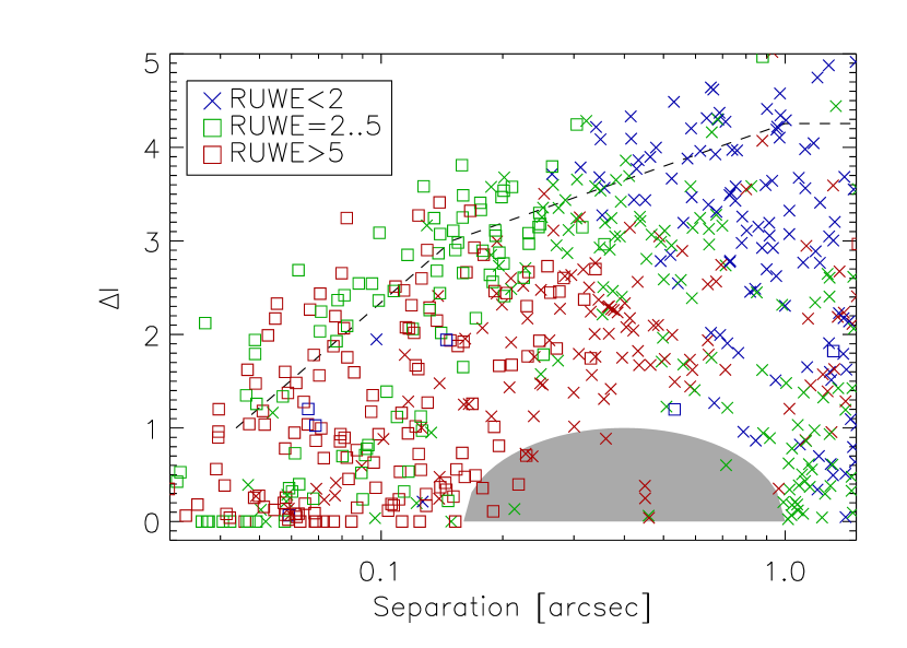
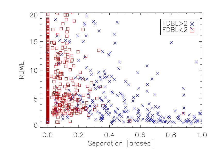
Figure 6: Comparison between SOAR resolutions of candidate subsystems and Gaia binarity flags. Top: magnitude difference $\Delta I$ vs. separation for resolved pairs. Crosses indicate FDBL$>$2 (effectively resolved by Gaia), and the squares mark FDBL$<$2. The colors show RUWE: $<$2 (blue), between 2 and 5 (green), and $>$5 (red). The gray shade indicates the Gaia avoidance of binaries, the dashed line is the median detection limit. Bottom: RUWE vs. angular separation. The blue crosses and red squares distinguish targets by FDBL.

3.3 SOAR Resolutions vs. Gaia Binarity Flags

The top panel of Figure 6 is a separation–contrast plot for the resolved subsystems. At the same time, it compares with the Gaia binarity flags (crosses with FDBL$>$2 are effectively resolved by Gaia, squares have single transits), while colors code the RUWE. Essentially all pairs wider than 0$\farcs$2 (and some closer ones) are resolved by double transits. The widest and dimmest companions have small RUWEs (blue crosses) and are not revealed by this criterion. On the other hand, brighter companions with $\Delta I<2$ mag at separations of $\sim$0$\farcs$5 have red and green symbols, indicating that an elevated RUWE was likely caused by the perturbing light of those companions rather than by the slow orbital motion with estimated periods on the order of centuries. Pairs closer than 0$\farcs$1 are detected only by RUWE. The lower panel of Figure 6 gives a complementary view of the interplay between $\rho$, RUWE, and FDBL. One can note that all subsystems identified by the FDBL flag (blue crosses) are resolved at SOAR. In contrast, a large part of subsystems with elevated RUWEs remained unresolved (zero separation) either because they are too close or because the companions are too faint. Although some correlation between parameters of the resolved pairs $(\rho,\Delta I)$ and the Gaia binarity flags is incontestable, this is not a deterministic relation because additional factors (e.g. the number of Gaia transits) influence the Gaia binarity indicators.

Figure 6 (top) shows a deficit of pairs with magnitude differences below 1 mag and separations above 0$\farcs$2. This “Gaia hole” is caused by missing parallaxes of close binaries, as mentioned above, so these stars are not present in the GCNS. The lower envelope gives approximate limits of the hole in the $(\rho,\Delta I)$ space. It can be described crudely by a semi-circle centered at 0$\farcs$4 with a logarithmic width of 2.5$\times$ and a height of 1 mag:

$$[\log(\rho/0\farcs 4)/\log(2.5)]^{2}+(\Delta I)^{2}<1$$ (1)

(see the gray shading in Figure 6). However, the limits are fuzzy, apparently depending on the Gaia scanning law and source location (some binaries may be lucky in getting parallaxes, while other binaries with similar parameters are not). Note the crosses near $(0\farcs 4,0)$ — binaries where Gaia DR3 measured parallaxes of one or both components with comparable magnitudes. Knowing the shape of the Gaia hole and the binary statistics, one can estimate the number of stars missing from the GCNS.

The resolution of inner subsystems at SOAR enables estimation of masses and mass ratios (from absolute magnitudes, using standard relations for main-sequence stars), as well as periods (assuming that projected separation is statistically representative of the semimajor axis). The methods are explained in the MSC paper (Tokovinin, 2018a). All new hierarchies with resolved subsystems are added to the MSC, which holds additional parameters such as estimated masses, periods, astrometry, etc. This information is not duplicated here, only the new observations are reported in Table 1. The updated MSC is publicly available through Vizier (catalog J/ApJS/235/6) and at http://www.ctio.noirlab.edu/~atokovin/stars/.

4 Hierarchies with Inner Gaia Orbits

Another input to the statistics of nearby hierarchies is derived from the orbital solutions in the NSS catalog (Gaia Collaboration et al., 2022; Pourbaix et al., 2022). The NSS information is presented in 17 tables, separately for each solution type. Here, only the eight most frequent types are used, ignoring the rest (eclipsing binaries, circular orbits, etc.). The data were recovered from the Vizier catalog I/357 (Gaia Collaboration, 2022) and ingested into IDL structures. Note that the SB1 and SB2 tables in the NSS do not contain any astrometric information. The Gaia astrometry of spectroscopic binaries was recovered from the main DR3 catalog, linked to the NSS by the Gaia identifiers.

Table 2: NSS Solutions

Code	Solution	$N_{\rm mult}$	$N_{\rm GCNS}$
AORB	Orbital	251	2355
ASB1	AstroSpectroSB1	144	1400
SB1	SB1	231	1388
SB2	SB2	79	311
A7	Acceleration7	331	2398
A9	Acceleration9	221	1970
RV1	FirstDegreeTrendSB1	53	277
RV2	SecondDegreeTrendSB1	55	289
All	…	1365	10,388

Table 3: Resolved Subsystems with NSS Orbits

MSC	Comp.	Sol.	$\rho$	$\Delta I$	$P$	Comment
			(′′)	(mag)	(d)
01242$-$2157	A	ASB1	0.057	0.2	1734	Blended
04097$-$5256	A	AORB	0.176	3.4	121.9	Suspect
05130$-$8125	A	SB1	0.040	1.1	1192	Blended
05574$-$2458	A	SB1	0.467	3.1	378	Suspect
07058$-$5849	A	SB1	0.052	2.0	1310	OK
07530$-$0201	A	SB1	0.199	2.3	1.5	Wrong
07543+0232	A	SB1	0.364	2.3	36.6	Quintuple?
09336$-$2752	A	SB2	0.139	2.9	37.5	Quadruple?
10356$-$4715	A	ASB1	0.026	0.0	547.4	Blended
12022$-$4844	A	SB1	0.095	3.1	52.0	Quadruple?
15229$-$6242	B	AORB	0.047	0.7	1421	OK, moves
15397$-$4956	A	SB1	0.046	0.8	44.8	Suspect
16412+0349	A	SB1	0.057	1.3	1034	Blended
19221$-$0444	B	AORB	0.086	1.6	2624	OK
19369$-$6949	A	ASB1	0.023	0.0	735	Blended
20147$-$7252	A	SB1	0.253	3.5	305.9	Suspect
21320$-$0129	B	ASB1	0.030	0.7	1056	Blended
21460$-$5233	A	SB1	0.088	2.5	28.6	Suspect
22170+1824	B	SB1	0.366	2.0	11.9	Quadruple?
22377$-$0210	A	SB1	0.049	1.7	7.0	Quadruple

Table 2 gives the short codes adopted here for the NSS solutions, their official self-explanatory names, the number $N_{\rm mult}$ of such solutions found among wide binaries, and their total number $N_{\rm GCNS}$ in the GCNS. The first four types provide orbital elements and thus are relevant for the statistics. Those 705 subsystems were matched to the MSC and added to it, if missing. The other half of the solutions (660) give only accelerations or radial velocity (RV) trends; they do not constrain the inner mass ratios, while the periods likely exceed 1000 days. The total number of NSS solutions for the GCNS objects is 10,388, or 3.1%. The number of solutions for the 50,243 members of wide pairs or triples is 1365, or 2.7%. By construction, the NSS catalog tried to avoid close companions, explaining its slightly lower rate of solutions for stars belonging to wide binaries.

The total numbers of stars with RUWE$>$2 (candidates for astrometric orbits) are 40,336 and 6995 in the full GCNS and in our list of 50,243 stars, respectively. The numbers of astrometric (AORB and ASB1) orbits in Table 2, 395 and 3755, are much smaller, only 9.3% and 5.6% of stars with RUWE$>$2. The speckle survey suggests that half of the RUWE-selected candidates can be resolved, so that their long periods are not yet covered by the NSS. Still, the estimated $\sim$19% completeness of astrometric orbits for the remaining half is quite low.

There are 318 matches between Nthe SS solutions and speckle targets, and 36 of those are resolved by SOAR at separations below 1″. The resolution rate of 11% is substantially lower than for the whole speckle survey (48%). Only 20 resolved subsystems have orbital elements in the NSS. However, the detailed comparison in Table 3 casts doubts on some orbits. Close companions perturb Gaia astrometry and the RVs measured by its slitless spectrograph, leading to suspicious orbits. For example, the orbit of 07530$-$0201 A with $P=1.5$ days and amplitude $K_{1}=1$ km s^-1 , if true, would imply an unlikely substellar companion in the brown dwarf desert regime, so the period seems spurious. Suspicious orbits with periods close to a year or its harmonics could result from the companion-induced effects that vary in a regular way throughout the year, following the Gaia scanning direction. Some spectroscopic orbits with periods on the order of a month or shorter could be real, indicating that the companion resolved by SOAR (with estimated periods of a few years or decades) orbits an inner spectroscopic binary, while the resolved Gaia companion is on a still wider outer orbit (a quadruple of 3+1 hierarchy). However, the possibility that some of those spectroscopic orbits are wrong still remains, and follow-up RV monitoring is needed for their verification.

In eight resolved subsystems the periods estimated from the separations approximately match the NSS orbital periods. However, the amplitude of the RV variation or the astrometric semimajor axis are often reduced by blending of comparable-brightness stars, as follows from the measured magnitude differences. The mass ratios derived from the blended NSS orbits are in fact lower limits. Several speckle measurements of 10356$-$4715 and 19369$-$6949 taken during one year show rapid motion compatible with their 2 yr orbits.

The uniform and impersonal coverage of Gaia orbits offers a definitive advantage for statistical studies. However, the automatic orbit calculation and the cadence imposed by the Gaia scanning law lead to a non-negligible fraction of wrong orbits, despite efforts to remove them by the NSS creators.

5 Discussion

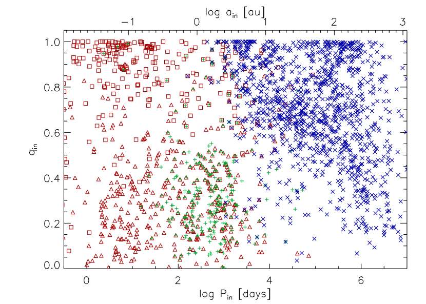
Figure 7: Periods and mass ratios of inner subsystems in known hierarchies within 100 pc. The SB1 and SB2 orbits are plotted by the red squares and triangles, respectively, astrometric orbits by green pluses, and resolved subsystems by blue crosses. The mass ratios of SB1s and astrometric binaries are lower limits. The upper axis gives orbital separations for a mass sum of 2 $M_{\odot}$ .

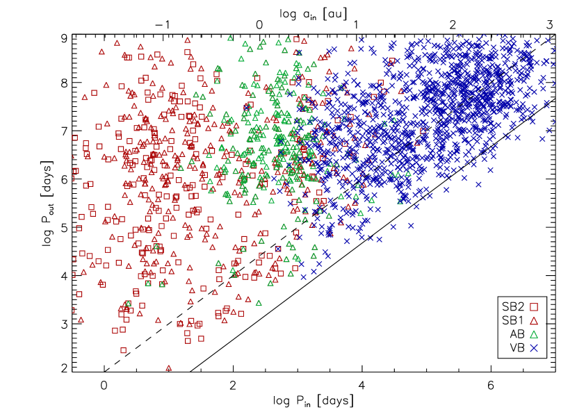
Figure 8: Periods in the inner and outer subsystems at adjacent hierarchical levels. The symbols correspond to the detection methods of inner subsystems, as in Figure 7. The solid and dash lines indicate the period ratios of 4.7 and 100, respectively.

After the addition of the newly resolved subsystems and subsystems with NSS orbits, the MSC contains 2,754 hierarchies within 100 pc with estimated periods. For the following discussion, I select from the MSC 2,208 systems within 100 pc with primary masses from 0.5 to 1.5 $M_{\odot}$ (excluding 77 systems containing known white dwarfs). Most of them are triples, while systems of four or more stars can be decomposed into elementary triples. Figure 7 plots the inner periods and mass ratios for this sample. The symbols distinguish the observing techniques and clearly separate the subsystems into groups. The upper right corner of the plot is occupied by the 1,280 resolved subsystems (blue crosses), including those studied here. Their lowest mass ratios depend on the period (or separation) owing to the limitation of the observing method (speckle and Gaia resolutions). The 243 double-lined spectroscopic binaries (red squares) occupy the upper-left corner, as expected. Most of the 444 single-lined spectroscopic (red triangles) and 273 astrometric (green pluses) binaries have periods shorter than 3 yr (duration of the Gaia DR3 observations), and their mass ratios are lower limits owing to blending. Orbital inclination also reduces the mass ratios of SB1s, but this is a smaller effect compared to the blending. Please, keep in mind that some NSS orbits are false.

The gaps between the three islands of points in Figure 7 are almost certainly caused by the observing techniques, rather than by a real dichotomy of the underlying population. Overlapping symbols correspond to simultaneous detections by several methods, but the number of such overlaps is quite modest. The density of points at short periods of $P_{\rm in}<1000$ days is less than in the area covered by the speckle detections, reflecting the small percentage of NSS orbits mentioned above. The plot gives a rough idea of the coverage of the parameter space and of the remaining incompleteness. For example, many subsystems with $a_{\rm in}\sim 10$ au and $q_{\rm in}<0.6$, below the speckle detection limit, are yet to be resolved by high-contrast imaging. Their orbital periods are longer than the duration of the Gaia mission.

Let us focus on the upper-right corner of Figure 7 ($P_{\rm in}>10^{4}$ days, $q_{\rm in}>0.6$), where the detection of subsystems by imaging is uniform. The observed distribution is thus representative of the real distribution of subsystems, and it has some interesting features worthy of comment. The concentration of points near $q_{\rm in}\approx 1$ is a well-known manifestation of twin binaries (it is even more prominent at shorter periods). A statistically significant excess of wide twin binaries with separations up to $10^{3}$ au has been detected by El-Badry et al. (2019). The recent study by Hwang et al. (2022) shows that wide twins with separations from 400 to $10^{3}$ au have extremely eccentric orbits, suggesting that they were formed as tighter 10–100 au pairs and later ejected to wide and eccentric orbits, presumably by dynamical interactions in unstable triples. In the light of this discovery, the abrupt decrease in the frequency of inner subsystems (including twins) at separations above $\sim$300 au, seen in Figure 7, appears natural (wider subsystems form rarely). This separation corresponds to 3″ at 100 pc distance, beyond the Gaia hole that ends at 1″. So, the paucity of wider inner subsystems is not caused by observational selection.

Detailed examination of these data reveals that most inner pairs with $q_{\rm in}\sim 1$ and separations from 10 to 100 au are missing from our list of candidate hierarchies because they fall in the Gaia hole (there are fewer points in this area of the plot). These hierarchies are known owing to historic ground-based efforts. One can also note a slight deficiency of wide inner subsystems with $q_{\rm in}\approx 0.8$. If the significance of this local minimum in the distribution of $q_{\rm in}$ is confirmed and proven not to result from observational biases, its explanation will present an interesting challenge to the theory of multiple-star formation.

Figure 8 is a standard plot comparing inner and outer periods in nearby hierarchies, with symbols coding the detection techniques of inner subsystems in the same way as above. The Gaia resolution limit of $\sim$1″ corresponds to 100 au or a period of $10^{5.5}$ days. The outer periods of the Gaia candidates studied here are located above this line, and one notes a reduced density of points below it, at shorter outer periods. This region of the parameter space where Gaia does not discover new hierarchies suffers from a larger incompleteness. Systematic discovery and characterization of compact hierarchies with outer separations below 100 au remains an outstanding observational challenge.

Some points in Figure 8 for resolved triples (blue crosses) fall below the dynamical stability limit $P_{\rm out}/P_{\rm in}>4.7$, depicted by the solid line. The periods are estimated only crudely from projected separations, explaining this apparent contradiction. Nevertheless, there is a substantial number of marginally stable or even unstable hierarchies. Marginally stable hierarchies with short periods $P_{\rm in}<100$ days are especially interesting because their non-Keplerian motion can be directly observed (see an example in Borkovits et al., 2019). Unfortunately, Gaia is of little help for the study of these fascinating objects because it was not designed for such work.

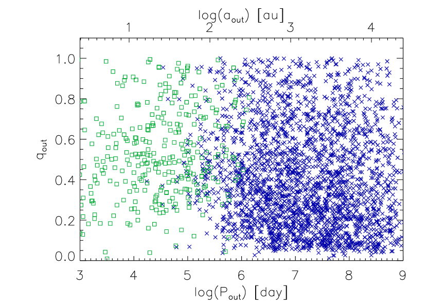
Figure 9: Periods and mass ratios in the outer subsystems of known hierarchies within 100 pc. The blue crosses denote wide (common PM) outer pairs, and the green squares correspond to other (mostly visual and speckle) discovery methods.

Figure 9 presents outer periods and mass ratios for hierarchies within 100 pc. Wide tertiary companions with $P_{\rm out}>10^{6}$ days have separations above 300 au (3″ at a 100 pc distance), therefore their detection by Gaia is quite complete, unlike closer companions detected by high-resolution imaging. A mild decrease of the outer mass ratio with increasing outer period is thus a real feature of nearby hierarchies, rather than a selection effect. The median $q_{\rm out}$ is 0.39 for $P_{\rm out}$ between $10^{6}$ and $10^{7}$ days; it decreases to 0.36 and 0.34 in the next two decades of outer periods. At outer periods below $10^{5.5}$ days, covered mostly by imaging techniques, large outer mass ratios are rare; the points group near $q_{\rm out}\sim 0.5$, as expected for triples composed of three similar-mass stars that are discovered more readily.

In this work, hierarchies are identified by searching for inner subsystems in wide binaries. Hwang (2023) did the opposite by looking for wide tertiary companions to close binaries with NSS orbital solutions. The wide-binary catalog of El-Badry et al. (2021) was used, and an outer separation range between 1 and 10 kau was considered. The sample was restricted to the main-sequence stars within 500 pc with masses from 0.8 to 1.4 $M_{\odot}$ . Such field stars have a 5.35% fraction of wide companions, but this fraction was found to be larger by 2.28$\pm$0.10 times for eclipsing binaries and by 1.33$\pm$0.05 times for SBs. The enhanced frequency of tertiary companions to close solar-type binaries discovered in Gaia data by Hwang confirms the earlier results (Tokovinin et al., 2006; Tokovinin, 2018a) and indicates that the formation of close and wide subsystems is somehow related.

For astrometric binaries, the frequency of tertiaries found by Hwang was only a 0.65$\pm$0.03 fraction of their frequency in the field. However, the presence of astrometric subsystems biases parallaxes and PMs, so many wide binaries with astrometric subsystems appear unbound and get excluded from the El-Badry’s catalog, which imposes the boundness condition. This pitfall is avoided here by using a relaxed criterion for wide-binary selection. Our sample of wide pairs has a relative frequency of 5.76% for the same range of masses (0.8 to 1.4 $M_{\odot}$ ) and separations (from 1 to 10 kau) as in Hwang (2023), slightly larger than 5.35% quoted in his paper. The number of astrometric subsystems with NSS solutions (AORB and ASB1) in these pairs is 38, or 2.5$\pm$0.5%, and the fraction of astrometric orbits in the full GCNS for this mass range is the same, 2.4$\pm$0.1%. I conclude that the depletion of astrometric orbits in wide pairs found by Hwang is not real, being caused by the inaccurate Gaia astrometry of stars with astrometric subsystems.

The GCNS hierarchies can clarify a long-standing issue concerning the frequency of 2+2 quadruples. Statistical modeling of the 67 pc sample of solar-type stars (Tokovinin, 2014) revealed that presence of inner subsystems in both components of wide pairs is correlated; otherwise, the number of predicted 2+2 quadruples would be less than observed. Such a conclusion had been reached earlier based on the presence of spectroscopic subsystems in wide binaries (Tokovinin & Smekhov, 2002). On the other hand, a similar study by Halbwachs et al. (2017) found no correlation between spectroscopic subsystems in components of 116 wide binaries.

I selected 15,983 pairs of two stars wider than 3″ from the list of 24,606 systems described above and determined the presence of subsystems in each component using either of the Gaia binarity indicators FDBL, RUWE, and RVERR, all with thresholds of 2. The numbers of subsystems in the primary, secondary, and both components are 3542, 2562, and 653, respectively (relative frequency 0.222, 0.160, and 0.041). If the presence of subsystems in both components is uncorrelated, the expected frequency of 2+2 quadruples is the product of subsystem frequencies in primaries and secondaries, $f_{2+2}=f_{1}f_{2}=0.0355$, while the observed frequency is 653/15,983=0.0408. The excess of 0.53%$\pm$0.16% is small but formally significant at the $3.3\sigma$ level. I repeated this test by setting a larger minimum separation or by using only two criteria, FDBL and RUWE, and obtained a comparable excess with significance above $2\sigma$. In a sample of 116 binaries, like the one of Halbwachs et al. (2017), such a small effect is lost in the noise. Interestingly, Fezenko et al. (2022) found that the simultaneous presence of eclipsing subsystems in both components of Gaia wide binaries is significantly enhanced compared to their frequency in the field.

6 Summary and Outlook

Combination of Gaia DR3 data with the ground-based speckle survey doubles the number of known hierarchical systems within 100 pc, reaching now almost 3,000. The estimated total number of such hierarchies is about 20,000, so our current knowledge is still very incomplete; some insights on the parameters of missing hierarchies are given above. Several thousand candidate nearby hierarchies were extracted from Gaia, but for most of them the parameters of inner subsystems remain unknown, while the outer separations are typically above 100 au. The main results of this work are:

1. A list of 8,032 candidate hierarchical systems within 100 pc based on the GCNS has been created.

2. A subset of 1,243 candidate hierarchies brighter than $G=12$ mag were observed by speckle interferometry at the 4.1 m telescope, and 506 close inner pairs were resolved.

3. New hierarchies are added to the MSC, doubling the number of known multiples within 100 pc. The resolved inner subsystems and those with NSS orbits occupy different regions of the period–mass ratio parameter space, with little overlap.

4. The amplitudes of Gaia SB1 and astrometric orbits are reduced by blending, hence the mass ratios derived from those orbits are lower limits.

Continued speckle monitoring of the newly discovered subsystems is needed for several reasons. Orbits of the closest and fastest inner pairs with estimated periods of a few years can be determined soon, filling the gap between visual and spectroscopic/astrometric orbits; the resolved Gaia orbital pairs from Table 3 are primary candidates. Re-observation of the remaining inner pairs within several years will define the direction and speed of their orbital motion. Its comparison with the motion in the outer pairs, accurately measured by Gaia, will give precious material for the statistical study of relative orbit orientation and eccentricity distribution; an example of such analysis for resolved Gaia triples can be found in Tokovinin (2022a), see also Hwang et al. (2022). Of special interest will be a dynamical study of marginally stable compact triples with comparable separations, like those in Figure 5.

A large sample of hierarchies with quantified observational selection is a starting point for inferring the true underlying distributions of their parameters (e.g. Tokovinin, 2014). The limits of speckle detection are well known, but the SOAR survey covers only a tiny fraction of the GCNS population. The sensitivity of Gaia binarity indicators is still poorly understood, although speckle interferometry helps in this respect. The selection effects in the NSS catalog are even more severe. Despite these obvious difficulties, the prospect of establishing unbiased statistics of binaries and hierarchies in the nearby field population is clear.

References

- Belokurov et al. (2020) Belokurov, V., Penoyre, Z., Oh, S., et al. 2020, MNRAS, 496, 1922, doi: 10.1093/mnras/staa1522
- Borkovits et al. (2019) Borkovits, T., Sperauskas, J., Tokovinin, A., et al. 2019, MNRAS, 487, 4631, doi: 10.1093/mnras/stz1510
- Bressan et al. (2012) Bressan, A., Marigo, P., Girardi, L., et al. 2012, MNRAS, 427, 127, doi: 10.1111/j.1365-2966.2012.21948.x
- El-Badry et al. (2021) El-Badry, K., Rix, H.-W., & Heintz, T. M. 2021, MNRAS, 506, 2269, doi: 10.1093/mnras/stab323
- El-Badry et al. (2019) El-Badry, K., Rix, H.-W., Tian, H., Duchêne, G., & Moe, M. 2019, MNRAS, 489, 5822, doi: 10.1093/mnras/stz2480
- Fezenko et al. (2022) Fezenko, G. B., Hwang, H.-C., & Zakamska, N. L. 2022, MNRAS, 511, 3881, doi: 10.1093/mnras/stac309
- Gaia Collaboration (2022) Gaia Collaboration. 2022, VizieR Online Data Catalog, I/357
- Gaia Collaboration et al. (2021a) Gaia Collaboration, Brown, A. G. A., Vallenari, A., et al. 2021a, A&A, 649, A1, doi: 10.1051/0004-6361/202039657
- Gaia Collaboration et al. (2016) —. 2016, A&A, 595, A2, doi: 10.1051/0004-6361/201629512
- Gaia Collaboration et al. (2021b) Gaia Collaboration, Smart, R. L., Sarro, L. M., et al. 2021b, A&A, 649, A6, doi: 10.1051/0004-6361/202039498
- Gaia Collaboration et al. (2022) Gaia Collaboration, Arenou, F., Babusiaux, C., et al. 2022, arXiv e-prints, arXiv:2206.05595. https://arxiv.org/abs/2206.05595
- Halbwachs et al. (2017) Halbwachs, J. L., Mayor, M., & Udry, S. 2017, MNRAS, 464, 4966, doi: 10.1093/mnras/stw2683
- Hartman & Lépine (2020) Hartman, Z. D., & Lépine, S. 2020, ApJS, 247, 66, doi: 10.3847/1538-4365/ab79a6
- Hwang (2023) Hwang, H.-C. 2023, MNRAS, 518, 1750, doi: 10.1093/mnras/stac3116
- Hwang et al. (2022) Hwang, H.-C., El-Badry, K., Rix, H.-W., et al. 2022, ApJ, 933, L32, doi: 10.3847/2041-8213/ac7c70
- Hwang et al. (2020) Hwang, H.-C., Hamer, J. H., Zakamska, N. L., & Schlaufman, K. C. 2020, MNRAS, 497, 2250, doi: 10.1093/mnras/staa2124
- Lee et al. (2019) Lee, A. T., Offner, S. S. R., Kratter, K. M., Smullen, R. A., & Li, P. S. 2019, ApJ, 887, 232, doi: 10.3847/1538-4357/ab584b
- Mason et al. (2001) Mason, B. D., Wycoff, G. L., Hartkopf, W. I., Douglass, G. G., & Worley, C. E. 2001, AJ, 122, 3466, doi: 10.1086/323920
- Moe & Di Stefano (2017) Moe, M., & Di Stefano, R. 2017, ApJS, 230, 15, doi: 10.3847/1538-4365/aa6fb6
- Offner et al. (2022) Offner, S. S. R., Moe, M., Kratter, K. M., et al. 2022, arXiv e-prints, arXiv:2203.10066. https://arxiv.org/abs/2203.10066
- Penoyre et al. (2022) Penoyre, Z., Belokurov, V., & Evans, N. W. 2022, MNRAS, 513, 5270, doi: 10.1093/mnras/stac1147
- Pourbaix et al. (2022) Pourbaix, D., Arenou, F., Gavras, P., et al. 2022, Gaia DR3 documentation Chapter 7: Non-single stars, Gaia DR3 documentation, European Space Agency; Gaia Data Processing and Analysis Consortium. Online at ¡A href=“https://gea.esac.esa.int/archive/documentation/GDR3/index.html”¿https://gea.esac.esa.int/archive/documentation/GDR3/index.html¡/A¿, id. 7
- Raghavan et al. (2010) Raghavan, D., McAlister, H. A., Henry, T. J., et al. 2010, ApJS, 190, 1, doi: 10.1088/0067-0049/190/1/1
- Tokovinin (2014) Tokovinin, A. 2014, AJ, 147, 87, doi: 10.1088/0004-6256/147/4/87
- Tokovinin (2018a) —. 2018a, ApJS, 235, 6, doi: 10.3847/1538-4365/aaa1a5
- Tokovinin (2018b) —. 2018b, PASP, 130, 035002, doi: 10.1088/1538-3873/aaa7d9
- Tokovinin (2022a) —. 2022a, ApJ, 926, 1, doi: 10.3847/1538-4357/ac4584
- Tokovinin (2022b) —. 2022b, AJ, 163, 161, doi: 10.3847/1538-3881/ac5330
- Tokovinin & Cantarutti (2008) Tokovinin, A., & Cantarutti, R. 2008, PASP, 120, 170, doi: 10.1086/528809
- Tokovinin et al. (2022) Tokovinin, A., Mason, B. D., Mendez, R. A., & Costa, E. 2022, AJ, 164, 58, doi: 10.3847/1538-3881/ac78e7
- Tokovinin et al. (2006) Tokovinin, A., Thomas, S., Sterzik, M., & Udry, S. 2006, A&A, 450, 681, doi: 10.1051/0004-6361:20054427
- Tokovinin & Smekhov (2002) Tokovinin, A. A., & Smekhov, M. G. 2002, A&A, 382, 118, doi: 10.1051/0004-6361:20011586
- Vrijmoet et al. (2022) Vrijmoet, E. H., Tokovinin, A., Henry, T. J., et al. 2022, AJ, 163, 178, doi: 10.3847/1538-3881/ac52f6
- Zavada & Píška (2022) Zavada, P., & Píška, K. 2022, AJ, 163, 33, doi: 10.3847/1538-3881/ac34f9
- Ziegler et al. (2021) Ziegler, C., Tokovinin, A., Latiolais, M., et al. 2021, AJ, 162, 192, doi: 10.3847/1538-3881/ac17f6