Data-driven abstractions via adaptive refinements and a Kantorovich metric

Abstract

We introduce an adaptive refinement procedure for smart and scalable abstraction of dynamical systems. Our technique relies on partitioning the state space depending on the observation of future outputs. However, this knowledge is dynamically constructed in an adaptive, asymmetric way. In order to learn the optimal structure, we define a Kantorovich-inspired metric between Markov chains, and we use it to guide the state partition refinement. Our technique is prone to data-driven frameworks, but not restricted to.

We also study properties of the above mentioned metric between Markov chains, which we believe could be of broader interest. We propose an algorithm to approximate it, and we show that our method yields a much better computational complexity than using classical linear programming techniques.

I Introduction

Feedback control of dynamical systems is at the core of several techniques that have caused tremendous impact in several industries, being essential to important advancements in e.g. aerospace and robotics. Traditionally, these control techniques were model-based, relying on a complete mathematical model to perform controller design. With recent technological advancements, however, where a vast amount of data can be collected online or offline, the interest within the control community to study methods that leverage available data for feedback controller design has been reignited [1, 2, 3, 4].

In this paper, we focus on data-driven techniques for building abstractions of dynamical systems. We call these data-driven abstractions. Abstraction methods create a symbolic model [5, 6] that approximates the behavior of the original (the “concrete”) dynamics in a way that controllers designed for such a symbolic representation can be refined to a valid controller for the original dynamics [7]. Several recent research efforts started exploring the possibility of generating abstractions for dynamical systems from observations of the latter [8, 9, 10, 11, 12].

In [8], we show that memory-based Markov models can be built from trajectory data. Memory has been classically used as a tool to mitigate non-Markovian behaviors of the original dynamics [13, 14], a feature also explored in recent papers [13, 10]. Increasing memory allows us to create more precise representations of the original dynamics using Markov decision processes (MDPs) or Markov chains. Despite promising results, [8] does not offer an adaptive mechanism to compute the generated abstraction, and thus it faces the curse of dimensionality, as the number of possible observations grows exponentially with the memory length. In this paper, we further develop the techniques in [8] by proposing an adaptive state space partitioning to mitigate the curse of dimensionality.

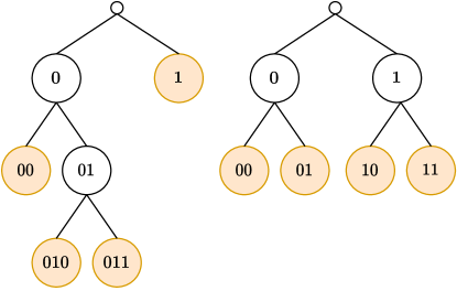
Figure 1: Difference between an adaptive and a brute-force approach. On the left, an adaptive approach: only some of the possible observations are expanded. On the right, a brute-force approach: every observation is expanded. The two resulting abstractions have four states, but the adaptive one provides a better abstraction (see Example 1).

A key contribution in this paper is the construction of a novel metric between two Markov chains; this metric is then exploited to adaptively increase memory in certain regions of the state space, in view of taming the complexity of the generated abstraction. An illustration of the difference between these two approaches is depicted in Figure 1. As opposed to [8], where states of the chain are associated with past memory, the abstractions we construct in this paper are based on forward memory. In order to define a metric between two Markov models, we leverage the Kantorovich metric (also known as the Wasserstein or Earth’s mover distance) between the induced probability on words of a fixed length and let the word length go to infinity. To define the Kantorovich metric, we equip the space of words with the Cantor distance, which is classically used in symbolic dynamics [5, 15]. We argue by means of numerical experiments that such a Kantorovich metric is natural and meaningful for control problems. We also show that the proposed metric is a well-defined and intuitive notion of similarity between Markov chains, and propose an algorithm for its computation that has better computational complexity over a naive application of linear programming techniques.

We believe that the proposed Kantorovich metric could be of much broader interest. Indeed, computing metrics between Markov models has been an active research topic within the computer science community [16]. Our construction on the metric between Markov chains resembles the one presented in [17], however with another distance. In [18] computability and complexity results are shown for the total variation metric. Kantorovich metrics for Markov models have been studied in [19, 20, 21, 22], but their underlying distance is different from ours. Our choice of the Cantor distance is crucial both for computational aspects and for building smart abstractions of dynamical systems.

Summarizing, our main contribution is threefold. First, we propose a new metric to measure distance between Markov models. Second, we develop an efficient algorithm that approximates arbitrarily well the proposed metric. Third, we exploit the proposed metric to adaptively improve abstractions in specific regions of the state space.

Outline

The rest of this paper is organized as follows. In Section II, we introduce the Kantorovich metric between two Markov chains, and propose an efficient algorithm to approximate it with arbitrary precision. In Section III, we apply this metric to build abstractions of dynamical systems using a greedy strategy that leads to the refinement of the state-space partitioning. We also demonstrate the quality of our procedure on an example.

Notations

Let $\mathcal{A}$ be a finite alphabet. We denote the set of $n$-long sequences of this alphabet by $\mathcal{A}^{n}$, and the set of countably infinite sequences by $\mathcal{A}^{*}$. The symbol $\Lambda$ stands for the empty sequence and, for any $w_{1}\in\mathcal{A}^{n_{1}}$, $w_{2}\in\mathcal{A}^{n_{2}}$, the sequence $w_{1}w_{2}\in\mathcal{A}^{n_{1}+n_{2}}$ is the concatenation of $w_{1}$ and $w_{2}$. Let $c(x)$ be a number of operations with respect to some attributes $x$. We say that an algorithm has a computational complexity $\mathcal{O}(f(x))$ if there exists $M>0$, $x_{0}$ such that, for all $x\geq x_{0}$, $c(x)\leq Mf(x)$. For any bounded set $X\subset\mathbb{R}^{d}$, let $\sigma(X)$ be the induced $\sigma$-algebra of $X$, and $\lambda$ be the Lebesgue measure on $\mathbb{R}^{d}$, then $\lambda_{X}:\sigma(X)\to[0,1]$ is defined as $\lambda_{X}(A)=\lambda(A)/\lambda(X)$. Finally, for any set $X$ and function $F$, the set $F(X)=\{F(x):x\in X\}$.

II A Kantorovich metric between Markov chains

In this section, a new notion of metric between Markov chains is defined. In Section III below, Markov chains will be used to represent abstractions of dynamical systems, and this distance will be used as a tool to construct adaptive abstractions. The present section, however, is concerned with Markov chains in their full generality.

II-A Preliminaries

Using a similar formalism as in [8], we define a labeled Markov chain as follows.

Definition 1 (Markov chain).

A Markov chain is a 5-tuple $\Sigma=(\mathcal{S},\mathcal{A},P,\mu,L)$, where $\mathcal{S}$ is a finite set of states, $\mathcal{A}$ is a finite alphabet, $P$ is the transition matrix on $\mathcal{S}\times\mathcal{S}$, $\mu$ is the initial measure on $\mathcal{S}$, and $L:\mathcal{S}\to\mathcal{A}$ is a labelling function.

In Definition 1, the entry of the transition matrix $P_{s,s^{\prime}}$ represents the probability $\mathbb{P}(X_{k+1}=s^{\prime}|X_{k}=s)$. The labelling $L$ induces a partition of the states. Consider the equivalence relation on $\mathcal{S}$ defined as $s\sim s^{\prime}$ if and only if $L(s)=L(s^{\prime})$. For any $a\in\mathcal{A}$, the notion of equivalent classes is defined as

$$[a]=\{s\in\mathcal{S}:L(s)=a\}.$$ (1)

We also define the behavior of a Markov chain $\mathcal{B}(\Sigma)\subseteq\mathcal{A}^{*}$ as follows. A sequence $w^{*}=(a_{1},a_{2},\dots)\in\mathcal{B}(\Sigma_{\mathcal{W}})$ if there exists $s_{1},s_{2},\dots\in\mathcal{S}$ such that $\mu_{s_{1}}>0$, $P_{s_{i},s_{i+1}}>0$ and $L(s_{i})=a_{i}$.

In the present work, we focus on a notion of metric between probabilities on label sequences. Let $w=(a_{1},\dots,a_{n})$ be a $n$-long sequence of labels, and define $p^{n}:\mathcal{A}^{n}\to[0,1]$ as

$$p^{n}(w)=\sum_{s_{1}\in[a_{1}]}\mu_{s_{1}}\sum_{s_{2}\in[a_{2}]}P_{s_{1},s_{2}}\dots\sum_{s_{n}\in[a_{n}]}P_{s_{n-1},s_{n}},$$ (2)

that is the probability induced by the Markov chain on $n$-long sequences.

Remark 1.

Classical procedures are well-known in the literature allowing to compute the probabilities $p^{n}$ for increasing $n$, with a complexity proportional to $|\mathcal{S}|^{2}$ at every step [23].

We endow the set of $n$-long sequences of labels with the Cantor distance $d_{B}$.

Definition 2 (Cantor’s distance, [15]).

The Cantor distance $d_{B}:\mathcal{A}^{n}\times\mathcal{A}^{n}\to\mathbb{R}$ is defined as $d_{B}(w_{1},w_{2})=2^{-l}$, where $l$ is the length of the longest common prefix. In other words, let $w_{1}=(a_{1},\dots,a_{n})$ and $w_{2}=(b_{1},\dots,b_{n})$, then $d_{B}(w_{1},w_{2})=2^{-l}$, where $l=\inf\{k:a_{k}\neq b_{k}\}$.

Remark 2.

It is well-known that the Cantor distance is an ultrametric. It means that is satisfies the strong triangular inequality

$$d_{B}(w_{1},w_{3})\leq\max\{d_{B}(w_{1},w_{2}),d_{B}(w_{2},w_{3})\}.$$ (3)

This property will be crucial in our developments.

II-B The Kantorovich metric

Consider two Markov chains $\Sigma_{1}=(\mathcal{S}_{1},\mathcal{A},P_{1},\mu_{1},L_{1})$ and $\Sigma_{2}=(\mathcal{S}_{2},\mathcal{A},P_{2},\mu_{2},L_{2})$ defined on the same alphabet $\mathcal{A}$. For a fixed $n$, they generate the distributions $p^{n}_{1}$ and $p^{n}_{2}$ on the metric space $(\mathcal{A}^{n},d_{B})$ as described in (2).

Definition 3 (Kantorovich metric).

The Kantorovich metric between the probability distributions $p_{1}^{n}$ and $p_{2}^{n}$ is given by

$$K(p_{1}^{n},p_{2}^{n})=\min_{\pi^{n}\in\Pi(p_{1}^{n},p_{2}^{n})}\sum_{w_{1},w_{2}\in\mathcal{A}^{n}}d_{B}(w_{1},w_{2})\pi^{n}(w_{1},w_{2}),$$ (4)

where $\Pi(p_{1}^{n},p_{2}^{n})$ is the set of couplings of $p_{1}^{n}$ and $p_{2}^{n}$, which contains the joint distributions $\pi^{n}:\mathcal{A}^{n}\times\mathcal{A}^{n}\to[0,1]$ whose marginal distributions are $p_{1}^{n}$ and $p_{2}^{n}$, that is,

$$\begin{gathered}\forall w_{1},w_{2}\in\mathcal{A}^{n}:\,\pi^{n}(w_{1},w_{2})\geq 0,\\ \forall w_{1}\in\mathcal{A}^{n}:\,\sum_{w_{2}\in\mathcal{A}^{n}}\pi^{n}(w_{1},w_{2})=p_{1}^{n}(w_{1}),\\ \forall w_{2}\in\mathcal{A}^{n}:\,\sum_{w_{1}\in\mathcal{A}^{n}}\pi^{n}(w_{1},w_{2})=p_{2}^{n}(w_{2}).\end{gathered}$$ (5)

The Kantorovich metric is often interpreted as an optimal transport problem. Indeed one can see problem (4) as the problem of finding the optimal way to satisfy “demands” $p_{2}^{n}$ with “supplies” $p_{1}^{n}$, where the cost of moving $\pi^{n}(w_{1},w_{2})$ probability mass from $w_{1}$ to $w_{2}$ amounts to $\pi^{n}(w_{1},w_{2})d_{B}(w_{1},w_{2})$. An illustration is provided in Figure 2.

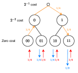
Figure 2: Interpretation of the Kantorovich distance as an optimal transport problem. In this example, the alphabet $\mathcal{A}=\{0,1\}$, $p_{1}^{2}(w)=1/4$ for all $w\in\mathcal{A}^{2}$, and $p_{2}^{2}(00)=0$, $p_{2}^{2}(01)=p_{2}^{2}(10)=1/4$, and $p_{2}^{2}(11)=1/2$. One can see that the optimal way to satisfy the demands $p_{2}^{n}$ with the supplies $p_{1}^{n}$ is to move $1/4$ of probability mass from $00$ to $11$, that is $\pi^{2}(00,11)=1/4$. Since $d_{B}(00,11)=1/2$, the Kantorovich distance is $K(p^{2}_{1},p^{2}_{2})=1/8$.

A naïve computation of $K(p_{1}^{n},p_{2}^{n})$ in (4) entails solving a linear program. However, standard techniques, such as interior point methods and network simplex result in some cases in a complexity of $\mathcal{O}(n|\mathcal{A}|^{3n}\log(|\mathcal{A}|))$, and therefore scale very poorly with the number labels. In this section, we show that it is possible to compute $K(p_{1}^{n},p_{2}^{n})$ in $\mathcal{O}(|\mathcal{S}|^{2}|\mathcal{A}|^{n+1})$ operations.

We first present two lemmata that will be useful for our purpose.

Lemma 1.

For any $n\geq 1$, let $\pi^{n}$ be the solution of (4). For all $w\in\mathcal{A}^{n}$,

$$\pi^{n}(w,w)=\min\{p_{1}^{n}(w),p_{2}^{n}(w)\}.$$ (6)

Lemma 2.

For any $n\geq 1$, let $\pi^{n+1}$ be the solution of (4). Then, for all $w\in\mathcal{A}^{n}$ such that $p^{n}_{1}(w)>p^{n}_{2}(w)$, then

$$\sum_{\begin{subarray}{c}w^{\prime}\in\mathcal{A}^{n}\\ w^{\prime}\neq w\end{subarray}}\sum_{a_{1},a_{2}\in\mathcal{A}}\pi^{n+1}(wa_{1},w^{\prime}a_{2}) =p^{n}_{1}(w)-p^{n}_{2}(w),$$ (7)

$$\sum_{\begin{subarray}{c}w^{\prime}\in\mathcal{A}^{n}\\ w^{\prime}\neq w\end{subarray}}\sum_{a_{1},a_{2}\in\mathcal{A}}\pi^{n+1}(w^{\prime}a_{1},wa_{2}) =0,$$

and for all $w_{1}\in\mathcal{A}^{n}$ such that $p_{1}^{n}(w_{1})\leq p_{2}^{n}(w_{1})$,

$$\sum_{\begin{subarray}{c}w^{\prime}\in\mathcal{A}^{n}\\ w^{\prime}\neq w\end{subarray}}\sum_{a_{1},a_{2}\in\mathcal{A}}\pi^{n+1}(wa_{1},w^{\prime}a_{2}) =0,$$ (8)

$$\sum_{\begin{subarray}{c}w^{\prime}\in\mathcal{A}^{n}\\ w^{\prime}\neq w\end{subarray}}\sum_{a_{1},a_{2}\in\mathcal{A}}\pi^{n+1}(w^{\prime}a_{1},wa_{2}) =p^{n}_{2}(w)-p^{n}_{1}(w).$$

We present in Theorem 1 a key result for writing an efficient algorithm. Due to space constraints, all the proofs are in the appendices of this paper.

Theorem 1.

For any $n\geq 1$, let $\pi^{n}$ be the solution of (4). Then the following holds:

$$K(p_{1}^{n+1},p_{2}^{n+1})=K(p_{1}^{n},p_{2}^{n})$$ (9)

$$+2^{-(n+1)}\sum_{w\in\mathcal{A}^{n}}\left[r(w)-\sum_{a\in\mathcal{A}}r(wa)\right],$$

where

$$r(w) =\min\{p_{1}^{n}(w),p_{2}^{n}(w)\},$$

$$r(wa) =\min\{p_{1}^{n+1}(wa),p_{2}^{n+1}(wa)\}.$$

Theorem 1 allows to prove that Algorithm 1 efficiently computes the Kantorovich metric between $p_{1}^{n}$ and $p_{2}^{n}$.

Algorithm 1 $\textsc{Kant}(k,m,w,n)$

for $i=1,\dots,|\mathcal{A}|$ do

     Compute $p_{1}^{n}(wa_{i})$ and $p_{2}^{n}(wa_{i})$ (see Remark 1)

     $r_{i}\leftarrow\min\{p_{1}^{n}(wa_{i}),p_{2}^{n}(wa_{i})\}$

$\textsc{res}=2^{-(k+1)}(m-\sum_{i=1,\dots,|\mathcal{A}|}r_{i})$

if $k+1=n$ then

     return res

for $i=1,\dots,|\mathcal{A}|$ do

     if $r_{i}\neq 0$ then

         $\textsc{res}\leftarrow\textsc{res}+\textsc{Kant}(k+1,r_{i},wa_{i},n)$      return res

Corollary 1.

Let Kant be the algorithm described in Algorithm 1, then

$$K(p^{n}_{1},p_{2}^{n})=\textnormal{{Kant}}(0,1,\Lambda,n).$$ (10)

Moreover Kant terminates in $\mathcal{O}(|\mathcal{S}|^{2}|\mathcal{A}|^{n+1})$ operations.

II-C A metric between Markov chains

Let $\Sigma_{1}$ and $\Sigma_{2}$ be two Markov chains defined on the same alphabet $\mathcal{A}$. We define a metric between them as

$$d(\Sigma_{1},\Sigma_{2})=\lim_{n\to\infty}K(p_{1}^{n},p_{2}^{n}),$$

where $p_{1}^{n}$ and $p_{2}^{n}$ are the distributions on $\mathcal{A}^{n}$ induced by each Markov chain on $n$-long label sequences.

Remark 3.

The Cantor distance $2^{-l}$ can be interpreted as a discount factor. Therefore, the metric $d(\Sigma_{1},\Sigma_{2})$, if well-defined, can be interpreted as a discounted measure of the difference between the behaviors $\mathcal{B}(\Sigma_{1})$ and $\mathcal{B}(\Sigma_{2})$.

We now prove that this metric is well-defined.

Theorem 2.

The metric $d(\Sigma_{1},\Sigma_{2})$ is well-defined. Moreover, for any $n\geq 1$,

$$0\leq d(\Sigma_{1},\Sigma_{2})-K(p_{1}^{n},p_{2}^{n})\leq 2^{-n}.$$

Theorem 2 provides a guarantee on the approximation of $d(\Sigma_{1},\Sigma_{2})$ that we will be able to compute. Indeed, for any $\varepsilon>0$, if $n\geq\lceil\log_{2}(\varepsilon^{-1})\rceil$, then $0\leq d(\Sigma_{1},\Sigma_{2})-K(p_{1}^{n},p_{2}^{n})\leq\varepsilon.$ Following Corollary 1, for a fixed number of labels and states, this implies that an $\varepsilon$-solution can be found in $\mathcal{O}(\varepsilon^{-1})$ computational complexity.

III Application to data-driven model abstractions

We now show how the metric $d(\Sigma_{1},\Sigma_{2})$ enables an adaptive refinement procedure for dynamical systems abstraction.

III-A Abstractions with adaptive refinement

In this section, we introduce a new abstraction based on adaptive refinements. Even though our approach can be generalized to stochastic systems, in this preliminary work we focus on deterministic ones, which we now define.

Definition 4 (Dynamical system).

A dynamical system is the $4$-tuple $S=(X,\mathcal{A},F,H)$ that defines the relation

$$x_{k+1}=F(x_{k}),\quad y_{k}=H(x_{k}),$$

where $X\subseteq\mathbb{R}^{d}$ is the state space, $\mathcal{A}$ is a finite alphabet called the output space, $F:X\to X$ is a transition function, and $H:X\to\mathcal{A}$ is the output function. The variables $x_{k}$ and $y_{k}$ are called the state and the output at time $k$.

Also, in parallel to the definition of behavior of a Markov chain, we define the behavior of a dynamical system $\mathcal{B}(S)\subseteq\mathcal{A}^{*}$ as follows. A sequence $w^{*}=(a_{1},a_{2},\dots)\in\mathcal{B}(S)$ if there exists $x_{1},x_{2},\dots\in X$ such that $x_{i+1}=F(x_{i})$ and $H(x_{i})=a_{i}$. Also, in parallel to equivalent classes (1) on Markov chains, we define equivalent classes on the continuous state space $X$. A subset of states is an equivalent class if it satisfies the recursive relation

$$[wa]_{S}=\{x\in[w]_{S}\,|\,H^{n}(x)=a\},\quad[\Lambda]_{S}=X,$$

for any $w\in\mathcal{A}^{n}$ and $a\in\mathcal{A}$. In other words, for a given sequence $w=(a_{1},\dots,a_{n})$, a state $x\in[w]_{S}$ if $H(x)=a_{1}$, $H(F(x))=a_{2}$, $\dots$, and $H(F^{n-1}(x))=a_{n}$. In this work, we impose the following assumption on dynamical systems.

Assumption 1.

The dynamical system $S$ as defined as Definition 4 is such that, for any $w\in\mathcal{A}^{n}$ and $a\in~\mathcal{A}$, the following two conditions hold:

• If $\lambda_{X}([w]_{S})=0$, then $[w]_{S}=\emptyset.$

• If $\lambda_{X}([wa]_{S})=\lambda_{X}([w]_{S})$, then $[w]_{S}=[wa]_{S}$.

Informally, Assumption 1 requires that any possible trajectory has a nonzero probability to be sampled.

Definition 5 (Adaptive partitioning).

Let $w_{1}\in\mathcal{A}^{n_{1}}$, $w_{2}\in\mathcal{A}^{n_{2}}$, $\dots$, $w_{k}\in\mathcal{A}^{n_{k}}$ be $k$ sequences of labels of different lengths. The set of sequences $\mathcal{W}=\{w_{i}\}_{i=1,\dots,k}$ is an adaptive partitioning for $S$ if

$$\bigcup_{w\in\mathcal{W}}[w]_{S}=X,\quad\forall i\neq j,\,[w_{i}]_{S}\cap[w_{j}]_{S}=\emptyset.$$

We now introduce an abstraction procedure based on an adaptive partitioning refinements.

Definition 6 (Abstraction based on adaptive refinements).

Let $S=(X,\mathcal{A},F,H)$ be a dynamical system as defined in Definition 4, and let $\mathcal{W}$ be an adaptive partitioning for $S$ as defined in Definition 5. Then the corresponding abstraction based on adaptive refinements is the Markov chain $\Sigma_{\mathcal{W}}=(\mathcal{S},\mathcal{A},P,\mu,L)$ defined as follows:

• The states are the partitions, that is $\mathcal{S}=\mathcal{W}$.

• $\mu_{w}$ is the Lebesgue measure of equivalent class $[w]_{S}$ on $X$, that is $\mu_{w}=\lambda_{X}([w]_{S})$.

• For $w_{1}=(a_{1},\dots,a_{n_{1}})$, and $w_{2}=(b_{1},\dots,b_{n_{2}})$, let $k=\min\{n_{1}-1,n_{2}\}$, $w_{1}^{\prime}=(a_{2},\dots,a_{k+1})$, and $w_{2}^{\prime}=(b_{1},\dots,b_{k})$. If $w_{1}^{\prime}\neq w_{2}^{\prime}$ or $\lambda_{X}([w_{1}]_{S})=0$, then $P_{w_{1},w_{2}}=0$. Else

  $$P_{w_{1},w_{2}}=\frac{\lambda_{X}([a_{1}w_{2}]_{S})}{\lambda_{X}([w_{1}]_{S})}.$$

• For $w=(a_{1},\dots,a_{n})$, $L(w)=a_{1}$.

Informally, for a given adaptive partitioning $\mathcal{W}$, the abstraction $\Sigma_{\mathcal{W}}$ can be interpreted as follows. The initial probability to be in the state $w$ in the Markov chain is the proportion of $[w]_{S}$ in $X$, and the probability to jump from the state $w_{1}$ to the state $w_{2}$ is the proportion of $[w_{1}]_{S}$ that goes into $[w_{2}]_{S}$ given the dynamics. For any sequence $w=(a_{1},\dots,a_{n})\in\mathcal{A}^{n}$, the probability $p^{n}(w)$ as defined in (2) is therefore the approximation for our abstraction of the probability that the output signal starts with the sequence $w$.

We now provide a result that gives a sufficient condition for the abstraction to have the same behavior as the original system.

Proposition 1.

Given a dynamical system $S$ satisfying Assumption 1, consider abstraction $\Sigma_{\mathcal{W}}$ as per Definition 6. If for all $w_{1},w_{2}\in\mathcal{W}$, $P_{w_{1},w_{2}}\in\{0,1\}$, then $\mathcal{B}(\Sigma_{\mathcal{W}})=\mathcal{B}(S)$.

III-B A data-driven abstraction

In this section, we propose a method to construct an abstraction based on adaptive refinements, from a data set comprising outputs sampled from the dynamical model $S$. Given an adaptive partitioning $\mathcal{W}$, we propose to construct $\Sigma_{\mathcal{W}}$ using empirical probabilities (see [8] for more details). We make the following assumption, which considers an idealised situation where one has an infinite number of samples. In practice, one typically has access to a finite number of observations, leading to approximation errors. The techniques to study these errors are investigated, for instance, in [10], and are left for further work in the context of this work.

Assumption 2.

For any abstraction $\Sigma_{\mathcal{W}}=(\mathcal{W},\mathcal{A},P,\mu,L)$, the transition probabilities $P$ and the initial distribution $\mu$ are known exactly.

Now we are able to use the tool investigated in Section II to find a smart adaptive partitioning. Indeed, one can construct two abstractions $\Sigma_{\mathcal{W}_{1}}$ and $\Sigma_{\mathcal{W}_{2}}$ corresponding to two different partitionings, and efficiently compute the Kantorovich metric $d(\Sigma_{\mathcal{W}_{1}},\Sigma_{\mathcal{W}_{2}})$ up to some accuracy $\varepsilon$ following Corollary 1. This gives a discounted measure of the difference between $\mathcal{B}(\Sigma_{\mathcal{W}_{1}})$ and $\mathcal{B}(\Sigma_{\mathcal{W}_{2}})$ (see Remark 3). This reasoning leads to the greedy procedure $\textsc{Refine}(S,N,\varepsilon)$ described in Algorithm 2.

Algorithm 2 $\textsc{Refine}(S,N,\varepsilon)$

$\mathcal{W}\leftarrow\{(a)\}_{a\in\mathcal{A}}$

Construct $\Sigma_{\mathcal{W}}$ from samples of $S$

while $\exists w_{1},w_{2}\in\mathcal{W}:P_{w_{1},w_{2}}\in(0,1)$ do

     if $N=0$ then

         return $\Sigma_{\mathcal{W}}$      

     for $i=1,\dots,|\mathcal{W}|$ do

         $\mathcal{W}_{i}^{\prime}\leftarrow\mathcal{W}\setminus\{w_{i}\}$

         $\mathcal{W}_{i}^{\prime}\leftarrow\mathcal{W}_{i}^{\prime}\cup\{w_{i}a\}_{a\in\mathcal{A}}$

         Construct $\Sigma_{\mathcal{W}^{\prime}_{i}}$ from samples of $S$

         $d_{i}\leftarrow d(\Sigma_{\mathcal{W}},\Sigma_{\mathcal{W}^{\prime}_{i}})$ with precision $\varepsilon$      

     $j=\arg\max_{i=1,\dots,|\mathcal{W}|}d_{i}$

     $\mathcal{W}\leftarrow\mathcal{W}^{\prime}_{j}$

     $\Sigma_{\mathcal{W}}\leftarrow\Sigma_{\mathcal{W}^{\prime}_{j}}$

     $N\leftarrow N-1$ return $\Sigma_{\mathcal{W}}$

An interpretation of Algorithm 2 goes as follows. Let $\mathcal{W}$ be a coarse partitioning, and $\mathcal{W}^{\prime}_{1}$ and $\mathcal{W}^{\prime}_{2}$ be two more refined partitionings. If $d(\Sigma_{\mathcal{W}},\Sigma_{\mathcal{W}^{\prime}_{1}})>d(\Sigma_{\mathcal{W}},\Sigma_{\mathcal{W}^{\prime}_{2}})$, then one could argue that it is more interesting to choose $\mathcal{W}^{\prime}_{1}$ over $\mathcal{W}^{\prime}_{2}$, since the discounted measure between the behaviors corresponding to the coarse partitioning and the refined partitioning is larger. Moreover, if at some point $\Sigma_{\mathcal{W}}$ is such that $P_{w,w^{\prime}}\in\{0,1\}$ for all $w,w^{\prime}\in\mathcal{A}^{n}$, then one has a sufficient condition to stop the algorithm following Proposition 1, otherwise the algorithm stops after $N$ iterations. If $N=\infty$, then the algorithm only stops in such case. An execution step of the algorithm can be found in Figure 3. A complexity analysis of Algorithm 2 can be found in Corollary 2.

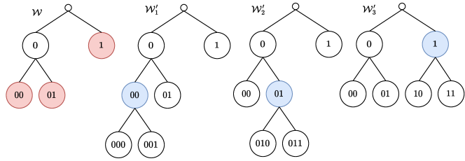
Figure 3: Illustration of the execution of Algorithm 2. Consider a current partitioning $\mathcal{W}=\{00,01,1\}$, with the corresponding abstraction $\Sigma_{\mathcal{W}}$. Then the algorithm will explore the partitionings $\mathcal{W}^{\prime}_{1}=\{000,001,01,1\}$, $\mathcal{W}^{\prime}_{2}=\{00,010,011,1\}$ and $\mathcal{W}^{\prime}_{3}=\{00,01,10,11\}$. For each one, it will compute $\Sigma_{\mathcal{W}^{\prime}_{i}}$, and $d(\Sigma_{\mathcal{W}},\Sigma_{\mathcal{W}^{\prime}_{i}})$, and choose the one for which the distance to $\Sigma_{\mathcal{W}}$ is the largest.

Corollary 2.

The algorithm $\textnormal{{Refine}}(S,N,\varepsilon)$ terminates in $\mathcal{O}(|\mathcal{A}|^{n+4}N^{4})$ operations, with $n=\lceil\log_{2}(\varepsilon^{-1})\rceil$. Moreover, for $S$ satisfying Assumption 1, if $\Sigma_{\mathcal{W}}=\textnormal{{Refine}}(S,\infty,\varepsilon)$ terminates, then $\mathcal{B}(\Sigma_{\mathcal{W}})=\mathcal{B}(S)$.

III-C Numerical examples

In this section, we demonstrate on an example that our greedy algorithm converges to a smart partitioning, and we show how to use the proposed framework for controller design.

Example 1.

Consider $S=(X,\mathcal{A},F,H)$ with $X=[0,2]\times[0,1]$, $\mathcal{A}=\{0,1\}$. Let $F$ be defined as

$$F(x)=\begin{cases}x&\textrm{if }x\in P_{1}\cup P_{4},\\ (x_{1}/2+1/2,x_{2}+1/2)&\textrm{if }x\in P_{2},\\ (x_{1}-1/2,x_{2})&\textrm{if }x\in P_{3},\\ (2x_{1}+1,4x_{2}-3/4)&\textrm{else},\end{cases}$$

where $P_{i}$ are depicted in Figure 4, and $H(x)=0$ if $x\in P_{1}$, else $H(x)=1$. An illustration and interpretation of $S$ is given in Figure 4.

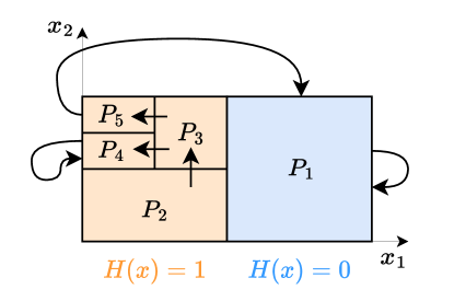
Figure 4: Illustration and description of the transition function $F$ of Example 1. $F$ has to be understood in the following way: $P_{1}$ is mapped to itself, $P_{2}$ is mapped to $P_{3}$, the lower half of $P_{3}$ is mapped to $P_{4}$, the upper half of $P_{3}$ is mapped to $P_{5}$, $P_{5}$ is mapped to $P_{1}$, and $P_{4}$ to itself.

The result of the algorithm applied to Example 1 at all iterations $k$ is depicted in Table I, and the final partitioning is illustrated in Figure 5. Observe that the generated partitioning aligns well with the dynamics, and that our algorithm generates an emerging structure which is not trivial. The algorithm stops at the third iteration since the obtained abstraction is such that $P_{w,w^{\prime}}\in\{0,1\}$, which is a stopping criterion following Proposition 1, and has much less states than the brute force approach of [8].

	$\mathcal{W}$	$d(\Sigma_{\mathcal{W}},\Sigma_{\mathcal{W}^{\prime}_{j}})$	$P_{w,w^{\prime}}\in\{0,1\}$
$k=0$	$\{0,\textbf{1}\}$	$0.0015$	No
$k=1$	$\{0,10,\textbf{11}\}$	$0.0059$	No
$k=2$	$\{0,10,110,\textbf{111}\}$	$0.0039$	No
$k=3$	$\{0,10,110,1110,1111\}$	-	Yes

TABLE I: Results of Algorithm 2 for Example 1. For each iteration $k$, the current model is the abstraction corresponding to $\Sigma_{\mathcal{W}}$, and the chosen model is $\Sigma_{\mathcal{W}^{\prime}_{j}}$, with the largest distance $d(\Sigma_{\mathcal{W}},\Sigma_{\mathcal{W}_{j}^{\prime}})$. With $P$ the transition matrix of the current model, if for all $w,w^{\prime}\in\mathcal{A}^{n}$, $P_{w,w^{\prime}}\in\{0,1\}$, the algorithm stops.

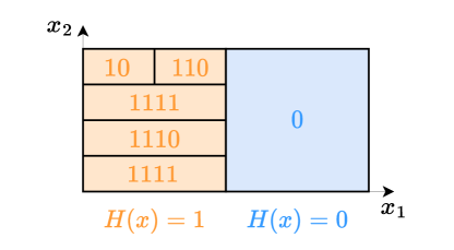
Figure 5: Illustration of the last partitioning $\mathcal{W}$ given by Algorithm 2 for Example 1.

We further demonstrate the quality of the obtained abstractions by designing a controller for a similar dynamical system.

Example 2.

Consider the dynamical system $S$ as described in Example 1, except that the dynamics is controlled as follows:

$$\tilde{x}_{k}=x_{k}+\begin{pmatrix}0\\ 1\end{pmatrix}u_{k},\quad x_{k+1}=F(\tilde{x}_{k})$$

where $u_{k}=K(x_{k})\in\{0,1/4,1/2\}$ is an input to the system. Consider the reward $r(x)=1$ if $H(x)=0$, else $r(x)=0$, and a discounted expected reward maximization objective, that is

$$\max_{K}\mathbb{E}_{x_{1}\sim\mu(X)}\sum_{k}\gamma^{k}r(x_{k}),$$ (11)

where $\mu(X)$ is the uniform distribution on $X$, and $\gamma=0.95$ is a discount factor.

To solve this optimal control problem, we will use the abstractions constructed by Algorithm 2. For each partitioning $\mathcal{W}$ in Table I, we will construct the abstraction $\Sigma_{\mathcal{W}}^{u}$ corresponding to the actions given in Example 2, that is $u=0$, $u=1/4$ and $u=1/2$. We will then solve a Markov Decision Process (or MDP for short, see [24] for an introduction) maximizing the expected reward of the MDP. For this, we used the implementation of the value iteration algorithm implemented in the POMDPs.jl Julia package [25]. Now, let $P(s)$ be the optimal policy for the state $s$, we design the controller for the system 2 as follows: for $x_{k}\in[w]_{S}$, then

$$u_{k}=K(x_{k})=P(w).$$ (12)

For the different abstractions found by Algorithm 2, the corresponding expected rewards (11) for the original system controlled by (12) are given in Table II. One can see that the expected reward increases as our algorithm refines the state-space.

Iteration	Controller (12)	Expected reward (11)
$k=0$	$K(x)=\begin{cases}0&\textrm{if }x\in[0]_{S}\\ 0&\textrm{if }x\in[1]_{S}\end{cases}$	14.4784
$k=1$	$K(x)=\begin{cases}0&\textrm{if }x\in[0]_{S}\\ 0&\textrm{if }x\in[10]_{S}\\ 1/4&\textrm{if }x\in[11]_{S}\end{cases}$	18.8726
$k=2$	$K(x)=\begin{cases}0&\textrm{if }x\in[0]_{S}\\ 0&\textrm{if }x\in[10]_{S}\\ 0&\textrm{if }x\in[110]_{S}\\ 1/4&\textrm{if }x\in[111]_{S}\end{cases}$	19.0311
$k=3$	$K(x)=\begin{cases}0&\textrm{if }x\in[0]_{S}\\ 0&\textrm{if }x\in[10]_{S}\\ 0&\textrm{if }x\in[110]_{S}\\ 1/2&\textrm{if }x\in[1110]_{S}\\ 1/4&\textrm{if }x\in[1111]_{S}\end{cases}$	19.1022

TABLE II: Expected rewards (11) for the Example 2 controlled by (12). The iterations $k$ correspond to the iterations of Algorithm 2 represented in Table I. The optimal policy is found by solving MDPs corresponding to the three possible actions $u_{k}\in\{0,1/4,1/2\}$, and the expected reward (11) is approximated by sampling $5000$ trajectories of length $1000$. One can observe that the expected reward increases.

IV Conclusion and further research

Inspired by a recent interest in developing data-driven abstractions of dynamical systems, we proposed a state refinement procedure that relies on a Kantorovich metric between Markov chains. We leverage the Cantor distance in the space of behaviours of the generated abstraction and use it to define the proposed Kantorovich metric. A key feature of our approach is a greedy strategy to perform state refinement that leads to an adaptive and smart partition of the state space. We show promising results in some control problems.

As further research, we plan to design a smart stopping criterion for our refinement procedure. We would also like to investigate convergence properties of our method, in the same fashion as in [8, Theorem 8].

-A Proof of Lemma 1

We first prove that $\pi^{n}(w,w)\leq\min(p_{1}^{n}(w),p_{2}^{n}(w))$. Constraints (5) imply that, for all $w\in\mathcal{A}^{n}$,

$$p_{1}^{n}(w)=\pi^{n}(w,w)+\sum_{\begin{subarray}{c}w^{\prime}\in\mathcal{A}^{n}\\ w^{\prime}\neq w\end{subarray}}\pi^{n}(w,w^{\prime})\geq\pi^{n}(w,w),$$ (13)

$$p_{2}^{n}(w)=\pi^{n}(w,w)+\sum_{\begin{subarray}{c}w^{\prime}\in\mathcal{A}^{n}\\ w^{\prime}\neq w\end{subarray}}\pi^{n}(w^{\prime},w)\geq\pi^{n}(w,w),$$

which imply that $\pi^{n}(w,w)\leq\min\{p_{1}^{n}(w),p_{2}^{n}(w)\}$. Now we prove that $\pi^{n}(w,w)\geq\min\{p_{1}^{n}(w),p_{2}^{n}(w)\}$. Consider an optimal solution $\pi^{n}$ to the problem (4) such that

$$\pi^{n}(w,w)=\min\{p_{1}^{n}(w),p_{2}^{n}(w)\}-\varepsilon,$$ (14)

for some $w\in\mathcal{A}^{n}$ and $\varepsilon>0$. Assume w.l.o.g. that $\min\{p_{1}(w),p_{2}(w)\}=p_{1}(w)$. Therefore, constraints (5) imply that

1. there exists $w^{\prime}\neq w$, such that $\pi^{n}(w,w^{\prime})=\varepsilon^{\prime}$ for some $\varepsilon^{\prime}\in(0,\varepsilon]$, and

2. there exists $w^{\prime\prime}\neq w$ such that $\pi^{n}(w^{\prime\prime},w)=\varepsilon^{\prime\prime}$ for some $\varepsilon^{\prime\prime}\in(0,\varepsilon]$.

Let $K(p_{1}^{n},p_{2}^{n})$ denote the Kantorovich metric corresponding to such $\pi^{n}$. Now assume w.l.o.g. that $\varepsilon^{\prime}\leq\varepsilon^{\prime\prime}$. Consider then $(\pi^{n})^{\prime}$ such that $(\pi^{n})^{\prime}(w_{1},w_{2})=\pi^{n}(w_{1},w_{2})$ for all $w_{1},w_{2}\in\mathcal{A}^{n}$ except

1. $(\pi^{n})^{\prime}(w,w)=\pi^{n}(w,w)+\varepsilon^{\prime}$,

2. $(\pi^{n})^{\prime}(w,w^{\prime})=\pi^{n}(w,w^{\prime})-\varepsilon^{\prime}$,

3. $(\pi^{n})^{\prime}(w^{\prime\prime},w^{\prime})=\pi^{n}(w^{\prime\prime},w^{\prime})+\varepsilon^{\prime}$, and

4. $(\pi^{n})^{\prime}(w^{\prime\prime},w)=\pi^{n}(w,w)-\varepsilon^{\prime}$.

The joint distribution $(\pi^{n})^{\prime}$ is feasible since it still satisfies the constraints (5). Now let $K^{\prime}(p_{1}^{n},p_{2}^{n})$ denote the solution corresponding to such $(\pi^{n})^{\prime}$, we have that

$$K^{\prime}(p_{1}^{n},p_{2}^{n})=K(p_{1}^{n},p_{2}^{n})$$ (15)

$$\quad-\varepsilon^{\prime}\left[d_{B}(w,w^{\prime})+d_{B}(w^{\prime},w^{\prime\prime})-d_{B}(w^{\prime},w^{\prime\prime})\right].$$

Since the Baire’s distance $d_{B}$ as defined in Definiton 2 satisfies triangular inequality, we have that $K^{\prime}(p_{1}^{n},p_{2}^{n})<K(p_{1}^{n},p_{2}^{n})$, which is a contradiction.

-B Proof of Lemma 2

For some $w\in\mathcal{A}^{n}$, assume w.l.o.g. that $p_{1}^{n}(w)>p_{2}^{n}(w)$. First, by feasibility conditions,

$$\sum_{\begin{subarray}{c}w^{\prime}\in\mathcal{A}^{n}\\ w^{\prime}\neq w\end{subarray}}\sum_{a_{1},a_{2}\in\mathcal{A}}\pi^{n+1}(wa_{1},w^{\prime}a_{2})\geq p_{1}^{n}(w)-p_{2}^{n}(w).$$ (16)

Now, we proceed similarly as for Lemma 1. Suppose by contradiction that

$$\sum_{\begin{subarray}{c}w^{\prime}\in\mathcal{A}^{n}\\ w^{\prime}\neq w\end{subarray}}\sum_{a_{1},a_{2}\in\mathcal{A}}\pi^{n+1}(wa_{1},w^{\prime}a_{2})>p_{1}^{n}(w)-p_{2}^{n}(w).$$ (17)

Then there exists $w^{\prime}\neq w\in\mathcal{A}^{n}$, and $a_{1},a_{2}\in\mathcal{A}$ such that $\pi^{n+1}(w^{\prime}a_{1},wa_{2})=\varepsilon^{\prime}>0$. There also exists $w^{\prime\prime}\in\mathcal{A}^{n}$ such that $w^{\prime\prime}\neq w$ and $w^{\prime\prime}\neq w^{\prime}$, and $a_{3},a_{4}\in\mathcal{A}$ such that $\pi^{n+1}(wa_{3},w^{\prime\prime}a_{4})=\varepsilon^{\prime\prime}>0$. Asumme w.l.o.g. that $\varepsilon^{\prime}\leq\varepsilon^{\prime\prime}$, and consider a solution $(\pi^{n+1})^{\prime}$ such that $(\pi^{n+1})^{\prime}=\pi^{n+1}$, except for

1. $(\pi^{n+1})^{\prime}(wa_{3},w^{\prime\prime}a_{4})=\pi^{n+1}(wa_{3},w^{\prime\prime}a_{4})-\varepsilon^{\prime}$,

2. $(\pi^{n+1})^{\prime}(w^{\prime}a_{1},wa_{2})=\pi^{n+1}(w^{\prime}a_{1},wa_{2})-\varepsilon^{\prime}$,

3. $(\pi^{n+1})^{\prime}(w^{\prime}a_{1},w^{\prime\prime}a_{4})=\pi^{n+1}(w^{\prime}a_{1},w^{\prime\prime}a_{4})+\varepsilon^{\prime}$, and

4. $(\pi^{n+1})^{\prime}(wa_{3},wa_{2})=\pi^{n+1}(wa_{3},wa_{2})+\varepsilon^{\prime}$.

The joint distribution $(\pi^{n+1})^{\prime}$ is feasible since it still satisfies the constraints (5). Note that, since the Baire’s distance satisfies the strong triangular inequality (see Remark 2),

$$d_{B}(w^{\prime}a_{1},w^{\prime\prime}a_{4}) \leq\max\{d_{B}(w^{\prime}a_{1},wa_{2}),d_{B}(wa_{2},w^{\prime\prime}a_{4})\}$$ (18)

$$=\max\{d_{B}(w^{\prime}a_{1},wa_{2}),d_{B}(wa_{3},w^{\prime\prime}a_{4})\}.$$

Moreover, $d_{B}(wa_{3},wa_{2})=2^{-(n+1)}$. Now let $K^{\prime}(p_{1}^{n+1},p_{2}^{n+1})$ denote the solution corresponding to such $(\pi^{n+1})^{\prime}$, we have that $K(p_{1}^{n+1},p_{2}^{n+1})-K^{\prime}(p_{1}^{n+1},p_{2}^{n+1})$ is

$$-\varepsilon^{\prime}\left[\begin{array}[]{ll}+&d_{B}(w^{\prime}a_{1},wa_{2})\\ +&d_{B}(wa_{3},w^{\prime\prime}a_{4})\\ -&d_{B}(w^{\prime}a_{1},w^{\prime\prime}a_{4})\\ -&2^{-(n+1)}\end{array}\right]$$ (19)

$$\leq-\varepsilon^{\prime}\left[\begin{array}[]{ll}+&d_{B}(w^{\prime}a_{1},wa_{2})+d_{B}(wa_{3},w^{\prime\prime}a_{4})\\ -&\max\{d_{B}(w^{\prime}a_{1},wa_{2}),d_{B}(wa_{3},w^{\prime\prime}a_{4})\}\\ -&2^{-(n+1)}\end{array}\right]$$

$$\leq-\varepsilon^{\prime}[2^{-n}-2^{-(n+1)}]$$

$$\leq 0,$$

which contradicts the fact that $\pi^{n+1}$ is optimal.

-C Proof of Theorem 1

For the sake of clarity, we note $K^{n}=K(p_{1}^{n},p_{2}^{n})$. We first prove that the right hand side of (9) is a lower bound for $K^{n+1}$. First we note that $K^{n+1}$ is equal to

$$\sum_{w_{1},w_{2}\in\mathcal{A}^{n}}\sum_{a_{1},a_{2}\in\mathcal{A}}d_{B}(w_{1}a_{1},w_{2}a_{2})\pi^{n+1}(w_{1}a_{1},w_{2}a_{2})$$ (20)

$$= \sum_{\begin{subarray}{c}w_{1},w_{2}\in\mathcal{A}^{n}\\ w_{1}\neq w_{2}\end{subarray}}d_{B}(w_{1},w_{2})\sum_{a_{1},a_{2}\in\mathcal{A}}\pi^{n+1}(w_{1}a_{1},w_{2}a_{2})$$

$$+2^{-(n+1)}\sum_{w\in\mathcal{A}^{n}}\sum_{\begin{subarray}{c}a_{1},a_{2}\in\mathcal{A}\\ a_{1}\neq a_{2}\end{subarray}}\pi^{n+1}(wa_{1},wa_{2})$$

$$:=C_{1}+C_{2}.$$

We first prove that $C_{1}\geq K^{n}$. To do this, let $\mu^{n}:\mathcal{A}^{n}\times\mathcal{A}^{n}\to[0,1]$ be defined as

$$\mu^{n}(w_{1},w_{2})=\sum_{a_{1},a_{2}\in\mathcal{A}}\pi^{n+1}(w_{1}a_{1},w_{2}a_{2}).$$ (21)

We show that $\mu^{n}$ satisfies the constraints (5). Indeed $\mu^{n}(w_{1},w_{2})\geq 0$,

$$\sum_{w_{2}\in\mathcal{A}^{n}}\mu(w_{1},w_{2}) =\sum_{w_{2}\in\mathcal{A}^{n}}\sum_{a_{1},a_{2}\in\mathcal{A}}\pi^{n+1}(w_{1}a_{1},w_{2}a_{2})$$ (22)

$$=\sum_{a_{1}}p_{1}^{n+1}(w_{1}a_{1})$$

$$=p_{1}^{n}(w_{1}),$$

and similarly for the third condition in (5). This implies that $\mu^{n}$ is a coupling, thereby a feasible solution of $\eqref{eq:kantorovich}$. This yields

$$K^{n}\leq\sum_{a_{1},a_{2}\in\mathcal{A}}d_{B}(w_{1},w_{2})\mu^{n}(w_{1},w_{2})=C_{1}.$$ (23)

Now we show that, for all $w\in\mathcal{A}^{n}$,

$$\sum_{\begin{subarray}{c}a_{1},a_{2}\in\mathcal{A}\\ a_{1}\neq a_{2}\end{subarray}}\pi^{n+1}(wa_{1},wa_{2})=r(w)-\sum_{a\in\mathcal{A}}r(wa),$$ (24)

which implies that

$$C_{2}=2^{-(n+1)}\sum_{w\in\mathcal{A}^{n}}\left[\sum_{w\in\mathcal{A}^{n}}r(w)-\sum_{a\in\mathcal{A}}r(wa)\right].$$ (25)

We prove the claim. Assume w.l.o.g. that $w$ is such that $p_{1}^{n}(w)>p_{2}^{n}(w)$, then

$$\sum_{a_{1},a_{2}\in\mathcal{A}}\pi^{n+1}(wa_{1},wa_{2})$$ (26)

$$=\sum_{a_{1}\in\mathcal{A}}\sum_{w^{\prime}\in\mathcal{A}^{n}}\sum_{a_{2}\in\mathcal{A}}\pi^{n+1}(wa_{1},w^{\prime}a_{2})$$

$$\quad\quad\quad\quad-\sum_{\begin{subarray}{c}w^{\prime}\in\mathcal{A}^{n}\\ w^{\prime}\neq w\end{subarray}}\sum_{a_{2}\in\mathcal{A}}\pi^{n+1}(wa_{1},w^{\prime}a_{2})$$

$$=\sum_{a_{1}\in\mathcal{A}}p_{1}^{n}(wa_{1})-\sum_{\begin{subarray}{c}w^{\prime}\in\mathcal{A}^{n}\\ w^{\prime}\neq w\end{subarray}}\sum_{a_{1},a_{2}\in\mathcal{A}}\pi^{n+1}(wa_{1},w^{\prime}a_{2})$$

Following Lemma 2, this is equal to

$$p_{1}^{n}(w)-\left(p_{1}^{n}(w)-p_{2}^{n}(w)\right)=r(w).$$ (27)

And the following holds:

$$\sum_{\begin{subarray}{c}a_{1},a_{2}\in\mathcal{A}\\ a_{1}\neq a_{2}\end{subarray}}\pi^{n+1}(wa_{1},wa_{2})$$ (28)

$$= \sum_{\begin{subarray}{c}a_{1}\neq a_{2}\in\mathcal{A}\\ a_{1}\neq a_{2}\end{subarray}}\pi^{n+1}(wa_{1},wa_{2})-\sum_{a\in\mathcal{A}}\pi^{n+1}(wa_{1},wa_{2})$$

$$= \,r(w)-\sum_{a\in\mathcal{A}}r(wa)$$

by Lemma 1. This concludes that the right hand side of (9) is a lower bound for $K^{n+1}$.

Now, to provide an upper bound, we will show that we can construct a feasible $n+1$ solution feasible $\mu^{n+1}$ such that

$$\sum_{w_{1},w_{2}\in\mathcal{A}^{n+1}}d_{B}(w_{1},w_{2})\mu^{n+1}(w_{1},w_{2})$$ (29)

$$\quad\quad\quad=K^{n}+\sum_{w\in\mathcal{A}^{n}}\left[r(w)-\sum_{a\in\mathcal{A}}r(wa)\right].$$

Consider $\pi^{n}$, an optimal solution at step $n$. We will construct $\mu^{n+1}$ in the following greedy way. Initialize $\mu^{n+1}$ with only zero elements, and for all $w\in\mathcal{A}^{n}$, $a\in\mathcal{A}$, we initialize $\delta(wa)=0$. We start by updating the blocks $\mu^{n+1}(w_{1}a_{1},w_{2}a_{2})$ where $w_{1}\neq w_{2}$. For all $w$ such that $p_{1}^{n}(w)>p_{2}^{n}(w)$, for all $a\in\mathcal{A}$ such that $p_{1}^{n+1}(wa)>p_{2}^{n+1}(wa)$, do the following.

1. Let $\tilde{\delta}(wa)=p_{1}^{n+1}(wa)-p_{2}^{n+1}(wa)$.
   If $\sum_{a^{\prime}\neq a}\delta(wa^{\prime})+\tilde{\delta}(wa)>p_{1}^{n}(w)-p_{2}^{n}(w)$, let $\delta(wa)=(p_{1}^{n}(w)-p_{2}^{n}(w))-\sum_{a^{\prime}\neq a}\delta(wa^{\prime})$.
   Else let $\delta(wa)=\tilde{\delta}(wa)$.

2. Find a $w^{\prime}\neq w$ such that

   $$\pi^{n}(w,w^{\prime})>\sum_{a_{1},a_{2}\in\mathcal{A}}\mu^{n+1}(wa_{1},w^{\prime}a_{2}).$$ (30)

   Now, for any $a^{\prime}\in\mathcal{A}$, let

   $$\psi(a^{\prime})=p_{2}^{n+1}(w^{\prime}a^{\prime})-p_{1}^{n+1}(w^{\prime}a^{\prime})$$ (31)

   $$-\sum_{\begin{subarray}{c}w^{\prime\prime}\in\mathcal{A}^{n}\\ w^{\prime\prime}\neq w^{\prime}\end{subarray}}\sum_{a_{1}\in\mathcal{A}}\mu^{n+1}(w^{\prime\prime}a_{1},w^{\prime}a^{\prime})$$

   Then, find $a^{\prime}\in\mathcal{A}$ such that $\psi(a^{\prime})>0$.
   Now, if $\delta(wa)>\psi(a^{\prime})$, then:

   • Update $\mu(wa,w^{\prime}a^{\prime})\leftarrow\psi(a^{\prime})$

   • Update $\delta(wa)\leftarrow\delta(wa)-\psi(a^{\prime})$

   • Return to 2.

   Else, update $\mu(wa,w^{\prime}a^{\prime})\leftarrow\delta(wa)$.

We claim that, in the procedure above, there always exists such a $w^{\prime}$ for a given $wa$. Otherwise,

$$\sum_{w^{\prime}\neq w}\pi^{n}(w,w^{\prime})<p_{1}^{n}(w)-p_{2}^{n}(w),$$ (32)

which is impossible by Lemma 1. Also, we claim that there also always exists such $a^{\prime}$ for a given $wa$ and $w^{\prime}$. Otherwise, for all $a^{\prime}\in\mathcal{A}$,

$$\sum_{a^{\prime}\in\mathcal{A}}\sum_{\begin{subarray}{c}w^{\prime\prime}\in\mathcal{A}^{n}\\ w^{\prime\prime}\neq w^{\prime}\end{subarray}}\sum_{a_{1}\in\mathcal{A}}\mu^{n+1}(w^{\prime\prime}a_{1},w^{\prime}a^{\prime})$$ (33)

$$\quad=\sum_{a^{\prime}\in\mathcal{A}}p_{2}^{n+1}(w^{\prime}a^{\prime})-p_{1}^{n+1}(w^{\prime}a^{\prime}),$$

which means by construction that

$$\sum_{a^{\prime}\in\mathcal{A}}\sum_{\begin{subarray}{c}w^{\prime\prime}\in\mathcal{A}^{n}\\ w^{\prime\prime}\neq w^{\prime}\end{subarray}}\sum_{a_{1}\in\mathcal{A}}\pi^{n+1}(w^{\prime\prime}a_{1},w^{\prime}a^{\prime})$$ (34)

$$\quad>\sum_{a^{\prime}\in\mathcal{A}}p_{2}^{n+1}(w^{\prime}a^{\prime})-p_{1}^{n+1}(w^{\prime}a^{\prime}),$$

which is $p_{2}^{n}(w)-p_{1}^{n}(w)>p_{2}^{n}(w)-p_{1}^{n}(w)$ by Lemma 2. Moreover, by construction we have that, for all $w\neq w^{\prime}$,

$$\pi^{n}(w,w^{\prime})=\sum_{a_{1},a_{2}\in\mathcal{A}^{n}}\mu^{n+1}(wa_{1},w^{\prime}a_{2}).$$ (35)

Now, we construct the diagonal blocks $\mu^{n+1}(wa_{1},wa_{2})$. For each $w\in\mathcal{A}^{n}$ and $a\in\mathcal{A}$, let

$$\begin{gathered}\tilde{p}_{1}^{n+1}(wa)=p_{1}^{n+1}(wa)-\sum_{w^{\prime}\neq w}\sum_{a\in\mathcal{A}}\mu^{n+1}(wa,w^{\prime}a^{\prime}),\\ \tilde{p}_{2}^{n+1}(wa)={p}_{2}^{n+1}(wa)-\sum_{w^{\prime}\neq w}\sum_{a\in\mathcal{A}}\mu^{n+1}(w^{\prime}a^{\prime},wa).\end{gathered}$$ (36)

Now, for a given $w$, let us solve the following balanced optimal transport problem:

$$\inf_{\mu^{n+1}}2^{-(n+1)}\sum_{\begin{subarray}{c}a_{1},a_{2}\in\mathcal{A}\\ a_{1}\neq a_{2}\end{subarray}}\mu^{n+1}(wa_{1},wa_{2})$$ (37)

s.t. $$\forall a_{1}\in\mathcal{A}:\,\sum_{a_{2}}\mu^{n+1}(wa_{1},wa_{2})=\tilde{p}_{1}^{n+1}(wa_{1}),$$

$$\forall a_{2}\in\mathcal{A}:\,\sum_{a_{1}}\mu^{n+1}(wa_{1},wa_{2})=\tilde{p}_{2}^{n+1}(wa_{2}).$$

Following the definition of $\tilde{p}$ and $\tilde{q}$, this is a balanced optimal transport whose trivial solution is given by

$$2^{-(n+1)}\left(r(w)-\sum_{a\in\mathcal{A}}r(wa)\right).$$ (38)

Now we conclude the proof. By (35) and (36), $\mu^{n+1}$ is a coupling of $p_{1}^{n+1}$ and $p_{2}^{n+1}$. Indeed it is positive, and for any $w_{1}\in\mathcal{A}^{n}$ and $a_{1}\in\mathcal{A}$,

$$\sum_{w_{2}\in\mathcal{A}^{n}}\sum_{a_{2}\in\mathcal{A}}\mu^{n+1}(w_{1}a_{1},w_{2}a_{2})$$ (39)

$$= \sum_{a_{2}\in\mathcal{A}}\mu^{n+1}(w_{1}a_{1},w_{1}a_{2})+\sum_{\begin{subarray}{c}w_{2}\in\mathcal{A}^{n}\\ w_{2}\neq w_{1}\end{subarray}}\sum_{a_{2}\in\mathcal{A}}\mu^{n+1}(w_{1}a_{1},w_{2}a_{2})$$

$$= \tilde{p}_{1}^{n+1}(w_{1}a_{1})+\left(p_{1}^{n+1}(w_{1}a_{1})-\tilde{p}_{1}^{n+1}(w_{1}a_{1})\right)$$

$$= p_{1}^{n+1}(w_{1}a_{1}),$$

and similarly for $p_{2}^{n+1}$. Finally,

$$\sum_{w_{1},w_{2}\in\mathcal{A}^{n}}\sum_{a_{1},a_{2}\in\mathcal{A}}d_{B}(w_{1}a_{1},w_{2}a_{2})\mu^{n+1}(w_{1}a_{1},w_{2}a_{2})$$ (40)

$$= \sum_{w_{1}\neq w_{2}}d_{B}(w_{1},w_{2})\sum_{a_{1},a_{2}}\mu^{n+1}(w_{1}a_{1},w_{2}a_{2})$$

$$+ 2^{-(n+1)}\sum_{w}\sum_{\begin{subarray}{c}{a_{1},a_{2}}\\ a_{1}\neq a_{2}\end{subarray}}\mu^{n+1}(wa_{1},wa_{2}).$$

By (35), the first term is $K^{n}$, and by (38), the second term is

$$\sum_{w\in\mathcal{A}^{n}}\left[r(w)-\sum_{a\in\mathcal{A}}r(wa)\right].$$ (41)

This provides an upper bound on $K^{n+1}$, and the proof is completed.

-D Proof of Corollary 1

We will prove that (10) holds by induction on the level of the execution tree of Algorithm 1. Let us prove that case $n=1$. The constraints (5) imply that

$$\sum_{a_{1},a_{2}\in\mathcal{A}}\pi^{1}((a_{1}),(a_{2}))=1.$$

Therefore,

$$K(p^{1}_{1},p^{1}_{2}) =2^{-1}\sum_{\begin{subarray}{c}a_{1},a_{2}\in\mathcal{A}\\ a_{1}\neq a_{2}\end{subarray}}\pi^{1}((a_{1}),(a_{2}))$$ (42)

$$=2^{-1}\left[1-\sum_{a\in\mathcal{A}}\pi^{1}((a),(a))\right].$$

Moreover, for all $a\in\mathcal{A}$, the solution of $\pi^{n}((a),(a))=r(wa)$ by Lemma 1. Therefore (42) is the result of $\textsc{Kant}(0,1,\Lambda,1)$. Now, assume that (10) holds for $n$. By Theorem 1,

$$K(p_{1}^{n+1},p_{2}^{n+1})=\textsc{Kant}(0,1,\Lambda,n)$$ (43)

$$\quad\quad+2^{-(n+1)}\sum_{w\in\mathcal{A}^{n}}\left[r(w)-\sum_{a\in\mathcal{A}}r(wa)\right].$$

Following the notations of Algorithm 1, let $m^{w}=r(w)$, and let $r_{i}^{w}=r(wa_{i})$. One can re-write (43) as

$$K(p_{1}^{n+1},p_{2}^{n+1})=\textsc{Kant}(0,1,\Lambda,n)$$

$$\quad\quad+\sum_{w\in\mathcal{A}^{n}}2^{-(n+1)}\left[m^{w}-\sum_{i=1,\dots,|\mathcal{A}|}r_{i}^{w}\right].$$

One can recognize $\textsc{Kant}(0,1,\Lambda,n+1)$ in the right hand side of the equation above, which conludes the proof of (10).

In terms of computational complexity, the bottleneck of Algorithm 1 is the computation of $p_{1}^{n}$ and $p_{2}^{n}$ at each node of the execution tree. Following Remark 1, this can be done in $\mathcal{O}(|\mathcal{S}|^{2})$ operations. Since there are $\mathcal{O}(|\mathcal{A}|^{n+1}|)$ nodes in the execution tree, the total number of operations is $\mathcal{O}(|\mathcal{S}|^{2}|\mathcal{A}|^{n+1})$.

-E Proof of Theorem 2

Let $K_{n}=K(p_{1}^{n},p_{2}^{n})$. First, we prove that, for all $n\geq 1$,

$$0\leq K_{n+1}-K_{n}\leq 2^{-(n+1)}.$$ (44)

Following Theorem 1, it suffices to show that

$$0\leq\sum_{w\in\mathcal{A}^{n}}\left[r(w)-\sum_{a\in\mathcal{A}}r(wa)\right]\leq 1,$$ (45)

By the law of total probability, we have that

$$p_{1}^{n}(w)=\sum_{a\in\mathcal{A}}p_{1}^{n+1}(wa),$$

and similarly for $p_{2}^{n}(w)$. Hence

$$0\leq r(w)-\sum_{a\in\mathcal{A}}r(wa)\leq r(w),$$

which shows that (45) holds. Now, notice that (44) implies that the sequence $(K_{n})_{n\geq 1}$ is monotone, and bounded since

$$\lim_{n\to\infty}K_{n} \leq K_{1}+\sum_{n\geq 1}(K_{n+1}-K_{n})$$

$$\leq 2^{-1}+\sum_{n\geq 1}2^{-(n+1)}$$

$$=1.$$

By the monotone convergence theorem, the limit exists and is equal to

$$\lim_{n\to\infty}K_{n}=\sup_{n\geq 1}K_{n}.$$

Moreover, since $K_{n}$ is a distance for every $n\geq 1$, and the limit exists, we have that $\lim_{n\to\infty}K_{n}$ is also a distance. Finally, by (44),

$$\lim_{n\to\infty}K_{n}-K_{p} =\left[K_{1}+\sum_{n=1}^{\infty}K_{n+1}-K_{n}\right]$$

$$\quad\quad\quad\quad\quad-\left[K_{1}+\sum_{n=1}^{p-1}K_{n+1}-K_{n}\right]$$

$$=\sum_{n\geq p}K_{n+1}-K_{n}$$

$$\leq\sum_{n\geq p}2^{-(n+1)}$$

$$=2^{-p}$$

for any $p\geq 1$, which concludes the proof of the theorem.

-F Proof of Proposition 1

We first prove that, if there are $w_{1},w_{2}\in\mathcal{W}$ such that $P_{w_{1},w_{2}}=1$, then

$$F([w_{1}]_{S})\subseteq[w_{2}]_{S}.$$ (46)

Let $w_{1}$, $w_{2}$, $k$, $w_{1}^{\prime}$ and $w_{2}^{\prime}$ be as in Definition 6. Let us note that

$$F([w_{1}]_{S}) =\left\{F(x)\in X\,\middle|\,\begin{array}[]{l}H(x)=a_{1},\\ H(F(x))=a_{2}\\ \dots\\ H(F^{n-1}(x))=a_{n_{1}}\end{array}\right\}$$ (47)

$$=F([(a_{1})]_{S})\cap[(a_{2},\dots,a_{n_{1}})]_{S}$$

Now, since $P_{w_{1},w_{2}}>0$, then $w_{1}^{\prime}=w_{2}^{\prime}$. There are two cases, either $w_{1}^{\prime}=(a_{2},\dots,a_{k+1})$ and $w_{2}^{\prime}=w_{2}$, or $w_{1}^{\prime}=w_{1}$ and $w_{2}^{\prime}=(b_{1},\dots,b_{k})$. Let us investigate these separately. In the first case, $(a_{2},\dots,a_{k+1})=w_{2}$. By definition,

$$[(a_{2},\dots,a_{n_{1}})]_{S}\subseteq[(a_{2},\dots,a_{k+1})]_{S}=[w_{2}]_{S}.$$

Therefore (47) implies

$$F([w_{1}]_{S})\subseteq F([(a_{1})]_{S})\cap[w_{2}]_{S}\subseteq[w_{2}]_{S},$$

which is (46). In the second case, assume that

$$[w_{1}]_{S}=[a_{1}w_{2}]_{S},$$ (48)

then

$$F([w_{1}]_{S}) =F([a_{1}w_{2}]_{S})$$

$$=F([(a_{1})]_{S})\cap[w_{2}]_{S}$$

$$\subseteq[w_{2}]_{S},$$

where a very similar as in (47) was used. It remains to show that (48) holds. Since we are in the second case cited above, then

$$a_{1}w_{2}=w_{1}(b_{k+1},\dots,b_{n_{2}}),$$

which implies that $[a_{1}w_{2}]_{S}\subseteq[w_{1}]_{S}$. Moreover, $P_{w_{1},w_{2}}=1$, that is

$$\lambda_{X}([a_{1}w_{2}]_{S})=\lambda_{X}([w_{1}]_{S}).$$

Following Assumption 1, it means that $[a_{1}w_{2}]_{S}=[w_{1}]_{S}$, which proves (46).

Now we prove that (46) implies $\mathcal{B}(\Sigma_{\mathcal{W}})=\mathcal{B}(S)$. We first prove that $\mathcal{B}(S)\subseteq\mathcal{B}(\Sigma_{\mathcal{W}})$. Let $w^{*}=(a_{1},a_{2},\dots)\in\mathcal{A}^{*}$ such that $w^{*}\notin\mathcal{B}(\Sigma_{\mathcal{W}})$, then there are $a_{i},a_{i+1}$ such that, for all $w_{1},w_{2}\in\mathcal{W}$ for which $L(w_{1})=a_{i}$ and $L(w_{2})=a_{i+1}$, $P_{w_{1},w_{2}}=0$. This could mean three things.

1. For all such $w_{1}$, $\lambda_{X}([(a_{i})]_{S})=0$. Following Assumption 1, it means that $[(a_{i})]_{S}=\emptyset$.

2. Let $w_{2}=(a_{i+1},b_{2},\dots,b_{n_{2}})$. For all such $w_{2}$,

   $$\lambda_{X}([(a_{i},a_{i+1},b_{2},\dots,b_{n_{2}})]_{S})=0,$$

   which means by Assumption 1 that

   $$[(a_{i},a_{i+1},b_{2},\dots,b_{n_{2}})]_{S}=\emptyset.$$

   By Definition 5, it implies that $[a_{i}a_{i+1}]_{S}=\emptyset$.

In any case, it means that $w^{*}\neq\mathcal{B}(S)$. Now we prove $\mathcal{B}(\Sigma_{W})\subseteq\mathcal{B}(S)$. Let $w^{*}=(a_{1},a_{2},\dots)\in\mathcal{B}(\Sigma_{\mathcal{W}})$. It means that there exists $w_{1},w_{2},\dots\in\mathcal{W}$ such that $L(w_{i})=a_{i}$ and $P_{w_{i},w_{i+1}}=1$. Following (46), this implies that $F([w_{i}]_{S})\subseteq[w_{i+1}]_{S}$. This implies that $[a_{i}a_{i+1}]_{S}\neq\emptyset$, which means $w^{*}\in\mathcal{B}(S)$.

-G Proof of Corollary 2

Proposition 1 gives a sufficient condition to stop the algorithm, hence the second part of the claim. It remains to prove that the computational complexity is the claimed one. Let $\mathcal{W}^{(k)}$ and $\mathcal{W}^{{}^{\prime}(k)}_{i}$ be the abstractions $\mathcal{W}$ and $\mathcal{W}_{i}^{\prime}$ at iteration $k$ in Algorithm 2. First we note that

$$|\mathcal{W}^{(k)}|=k|\mathcal{A}|-(k-1),\quad|\mathcal{W}^{{}^{\prime}(k)}_{i}|=(k+1)|\mathcal{A}|-k$$ (49)

At each iteration $k$, one has to compute $|\mathcal{W}^{(k)}|$ times the $\varepsilon$-accurate Kantorovich distance between two models of sizes given by (49). By Corollary 1, such computational complexity is

$$\mathcal{O}\left(|\mathcal{W}^{(k)}|\left(|\mathcal{A}|^{n+1}\left(|\mathcal{W}^{(k)}|^{2}+|\mathcal{W}^{{}^{\prime}(k)}_{i}|^{2}\right)\right)\right)$$

$$= \mathcal{O}\left(|\mathcal{A}|^{n+1}|\mathcal{W}^{{}^{\prime}(k)}_{i}|^{3}\right)$$

$$= \mathcal{O}\left(|\mathcal{A}|^{n+4}(k+1)^{3}\right).$$

Now, the worst-case is when the algorithm does not converge to an abstraction where there exists $w,w^{\prime}$ such that $P_{w,w^{\prime}}\in(0,1)$. Therefore, the total computational complexity is

$$\sum_{k=1}^{N}\mathcal{O}\left(|\mathcal{A}|^{n+4}(k+1)^{3}\right)=\mathcal{O}\left(|\mathcal{A}|^{n+4}N^{4}\right),$$

which is the claim.

References

- [1] C. D. Persis and P. Tesi, “Formulas for data-driven control: Stabilization, optimality, and robustness,” IEEE Transactions on Automatic Control, vol. 65, no. 3, pp. 909–924, mar 2020.
- [2] Z. Wang and R. M. Jungers, “A data-driven method for computing polyhedral invariant sets of black-box switched linear systems,” IEEE Control Systems Letters, vol. 5, no. 5, pp. 1843–1848, nov 2021.
- [3] J. Berberich, J. Kohler, M. A. Muller, and F. Allgower, “Data-driven model predictive control with stability and robustness guarantees,” IEEE Transactions on Automatic Control, vol. 66, no. 4, pp. 1702–1717, apr 2021.
- [4] A. Banse, Z. W. Raphael, and M. Jungers, “Black-box stability analysis of hybrid systems with sample-based multiple lyapunov functions,” in 2022 IEEE 61st Conference on Decision and Control (CDC). IEEE, dec 2022.
- [5] D. Lind and B. Marcus, An Introduction to Symbolic Dynamics and Coding. Cambridge University Press, nov 1995.
- [6] A. van der Schaft, “Equivalence of dynamical systems by bisimulation,” IEEE Transactions on Automatic Control, vol. 49, no. 12, pp. 2160–2172, dec 2004.
- [7] P. Tabuada, Verification and Control of Hybrid Systems. Springer US, 2009.
- [8] A. Banse, L. Romao, A. Abate, and R. Jungers, “Data-driven memory-dependent abstractions of dynamical systems,” in Proceedings of The 5th Annual Learning for Dynamics and Control Conference, ser. Proceedings of Machine Learning Research, N. Matni, M. Morari, and G. J. Pappas, Eds., vol. 211. PMLR, 15–16 Jun 2023, pp. 891–902. [Online]. Available: https://proceedings.mlr.press/v211/banse23a.html
- [9] A. Devonport, A. Saoud, and M. Arcak, “Symbolic abstractions from data: A PAC learning approach,” in 2021 60th IEEE Conference on Decision and Control (CDC). IEEE, dec 2021.
- [10] R. Coppola, A. Peruffo, and M. Mazo, “Data-driven abstractions for verification of linear systems,” IEEE Control Systems Letters, pp. 1–1, 2023.
- [11] A. Lavaei, S. Soudjani, E. Frazzoli, and M. Zamani, “Constructing MDP abstractions using data with formal guarantees,” IEEE Control Systems Letters, vol. 7, pp. 460–465, 2023.
- [12] T. Badings, L. Romao, A. Abate, D. Parker, H. A. Poonawala, M. Stoelinga, and N. Jansen, “Robust control for dynamical systems with non-gaussian noise via formal abstractions,” Journal of Artificial Intelligence Research, vol. 76, pp. 341–391, jan 2023.
- [13] R. Majumdar, N. Ozay, and A.-K. Schmuck, “On abstraction-based controller design with output feedback,” in Proceedings of the 23rd International Conference on Hybrid Systems: Computation and Control. ACM, apr 2020.
- [14] A.-K. Schmuck and J. Raisch, “Asynchronous -complete approximations,” Systems & Control Letters, vol. 73, pp. 67–75, nov 2014.
- [15] N. P. Fogg, V. Berthé, S. Ferenczi, C. Mauduit, and A. Siegel, Eds., Substitutions in Dynamics, Arithmetics and Combinatorics. Springer Berlin Heidelberg, 2002.
- [16] Y. Deng and W. Du, “The kantorovich metric in computer science: A brief survey,” Electronic Notes in Theoretical Computer Science, vol. 253, no. 3, pp. 73–82, nov 2009.
- [17] Z. Rached, F. Alajaji, and L. Campbell, “The kullback–leibler divergence rate between markov sources,” IEEE Transactions on Information Theory, vol. 50, no. 5, pp. 917–921, may 2004.
- [18] S. Kiefer, “On computing the total variation distance of hidden markov models,” 2018.
- [19] J. Desharnais, V. Gupta, R. Jagadeesan, and P. Panangaden, “Metrics for labelled markov processes,” Theoretical Computer Science, vol. 318, no. 3, pp. 323–354, jun 2004.
- [20] F. van Breugel, B. Sharma, and J. Worrell, “Approximating a behavioural pseudometric without discount for probabilistic systems,” in Foundations of Software Science and Computational Structures. Springer Berlin Heidelberg, 2007, pp. 123–137.
- [21] N. Madras and D. Sezer, “Quantitative bounds for markov chain convergence: Wasserstein and total variation distances,” Bernoulli, vol. 16, no. 3, aug 2010.
- [22] D. Rudolf and N. Schweizer, “Perturbation theory for markov chains via wasserstein distance,” Bernoulli, vol. 24, no. 4A, nov 2018.
- [23] L. Rabiner, “A tutorial on hidden markov models and selected applications in speech recognition,” Proceedings of the IEEE, vol. 77, no. 2, pp. 257–286, 1989.
- [24] R. S. Sutton and A. G. Barto, Reinforcement Learning: An Introduction. Cambridge, MA, USA: A Bradford Book, 2018.
- [25] M. Egorov, Z. N. Sunberg, E. Balaban, T. A. Wheeler, J. K. Gupta, and M. J. Kochenderfer, “POMDPs.jl: A framework for sequential decision making under uncertainty,” Journal of Machine Learning Research, vol. 18, no. 26, pp. 1–5, 2017. [Online]. Available: http://jmlr.org/papers/v18/16-300.html