Estimating Continuous Muscle Fatigue For Multi-Muscle Coordinated Exercise: A Pilot Study

Abstract

Assessing the progression of muscle fatigue for daily exercises provides vital indicators for precise rehabilitation, personalized training dose, especially under the context of Metaverse. Assessing fatigue of multi-muscle coordination-involved daily exercises requires the neuromuscular features that represent the fatigue-induced characteristics of spatiotemporal adaptions of multiple muscles and the estimator that captures the time-evolving progression of fatigue. In this paper, we propose to depict fatigue by the features of muscle compensation and spinal module activation changes and estimate continuous fatigue by a physiological rationale model. First, we extract muscle synergy fractionation and the variance of spinal module spikings as features inspired by the prior of fatigue-induced neuromuscular adaptations. Second, we treat the features as observations and develop a Bayesian Gaussian process to capture the time-evolving progression. Third, we solve the issue of lacking supervision information by mathematically formulating the time-evolving characteristics of fatigue as the loss function. Finally, we adapt the metrics that follow the physiological principles of fatigue to quantitatively evaluate the performance. Our extensive experiments present a 0.99 similarity between days, a over 0.7 similarity with other views of fatigue and a nearly 1 weak monotonicity, which outperform other methods. This study would aim the objective assessment of muscle fatigue.

Muscle fatigue, electromyography, muscle compensation, muscle synergy, spinal activation

1 Introduction

Muscle fatigue relates to the ability reduction of generating force or power after repetitive and intensive exercise [1]. Assessing muscle fatigue is of significant importance for sports, rehabilitation, human-robot interaction, even medical diagnosis areas [2, 3, 4, 5, 6]. Other than discretely classifying muscles are fatigued or not [7, 8, 9], depicting the continuous progression of muscle fatigue enables assessing to what extent muscles are fatigued, and would further benefit personalized dose determination, injury prevention, precise rehabilitation. Under the context of Metaverse, the depicted continuous fatigue progression can further provide a physiological indicator for remote and interactive rehabilitative training and aids physicians’ more fine-grained determination of dose and treatment, especially when combining with the VR/AR techniques. To do so, it is vital to propose an objective indicator that can form a fatigue score to continuously depict the muscle fatigue progression, especially during daily exercise that involves complex muscle coordination, i.e. sub-maximal and dynamic contractions of multiple muscles, like walking or running.

Extensive studies focus on noninvasive signal-extracted features that discretely reflect fatigue-induced changes of local muscle properties, without considering to form a continuous indicator. Fatigued muscles present changes of multiple physiological properties including lactic acid, blood oxygen metabolism, motor unit recruitment, and muscle fiber conduction velocity. Inspired by the phenomena of low frequency shift and increased amplitude, classical features like root mean square, median frequency and mean power frequency etc. are used to present temporal and spectral changes of electromyography (EMG) signals [8, 10]. High-density EMG decomposition further enables the detection of subtle muscle fibre properties, thus provides more precise features of local muscles [11, 7]. Besides, features from additional signals provide complementary information and are combined with EMG features. Taelman et al. [12] proposed to evaluate muscle fatigue by combining EMG features and tissue oxygenation features detected by near-infrared spectroscopy (NIRS). Studies like [13, 14] analyzed muscle fatigue through fusing EMG and mechanomyography (MMG). In this way, different aspects of muscle fibre activation can be included. Guo et al. [15] developed a sensor system that integrated EMG, MMG and NIRS, and further evaluated fatigue-sensitive features of each signal. Although inspiring, such studies solely focus on the fatigue-sensitive features and ignore the requirement of an estimator that fuses different features into a score to continuously depict fatigue progression. Moreover, such features are limited by their capability of reflecting local muscle properties, hardly considering the nervous system adaptations of multi-muscle coordination. Given the characteristics of complex daily movements that involve coordinated activation of multiple muscles, a more global feature integrating the neural control of multiple muscles would be beneficial.

Except for fatigue-sensitive features, an estimator is needed to fuse features and form a continuous fatigue score. Current methods mostly focus on static postures or isokinetic contractions of limited mucles. Monir et al. [16] utilized CNN to forecast EMG features of fatigued trunk muscles with the potential of estimating the binary fatigue states. Guo et al. [17] proposed a muscle fatigue estimator based on the weak monotonicity of features, which was able to form a continuous fatigue score estimator. Similarly, Yang et al. [18] trained a CNN to classify the onset of fatigue using signals of force plates and IMUs. Xu et al. [19] empirically estimated a fatigue index of isometric contraction and used it to modify force estimation. Rocha et al. [20] proposed an estimator based on the assumptions of the Markov chain and the stationary process. It estimated fatigue of isometric and isokinetic contractions by the deviation between the normalized features accumulation and the expectancy accumulation of a stationary process. Based on the same assumptions, Nascimento et al. [21] extended the framework and incorporated more features. Other than just focusing on static postures or isokinetic contractions, such methods are limited by their input local muscle features, and the stationary assumptions violate physiological priors of fatigue. The ability of accommodating daily movements that involve dynamic and sub-maximal multi-muscle coordination would be constrained.

In this study, we consider the comprehensive characteristics of muscle fatigue during multiple muscle-involved daily movements and use walking as the test bed. We propose to utilize features of muscle synergy fraction and spinal module activation in order to represent the temporal and spatial changes of multi-muscle activation caused by the fatigue-induced muscle compensation and spike timing deviations. We further synthesize the physiology-inspired features into a continuous fatigue score, in the manner of mathematically formulating the time-evolved nature and physiological characteristics of muscle fatigue as the loss function and the algorithmic architecture. To summarize, our contributions are as follows.

• To the best of our knowledge, this is the first study that can continuously assess muscle fatigue for the daily exercise scenarios involving submaximal and dynamic contractions of multiple muscles.

• We design physiology-inspired features to represent the fatigue-induced muscle compensation and spike timing deviations, in order to extract the global information of multi-muscle coordination.

• We develop a physiological rationale model and formulate the time-evolving dynamics of muscle fatigue as a novel loss function that solves the issue of lacking labels.

• We adapt the metrics of [22] to quantitatively evaluate our estimated fatigue and demonstrate it with extensive experiments.

2 Related Work

In order to develop a physiological rationale model for muscle fatigue, we review the physiological background, muscle level observations and evaluation paradigms related to muscle fatigue.

2.1 Key Concepts and Characteristics

Muscle fatigue is a multi-perspective concept and a whole body-involved process, which relates to the central command increase of motor regions, motoneuron spectral tuning, muscle fiber switch and motor performance alternation. There are three of the most prominent factors that we can utilize, i.e. 1) the supraspinal/spinal neuronal changes of temporal activation patterns, 2) the muscle compensation phenomenon and 3) task-specific fatigue performance. Specifically, repetitive activation of motoneurons and repetitive contractions of muscle fibers will induce reduced excitability of motoneuron itself and a supraspinal inhibition of motoneuron pool strengthened by group III/IV afferents and the short-latency reflex [23]. In addition, despite the increased motor command sent by motor cortex partially compensates for the fatigue-induced muscle fiber deactivation, the supraspinal fatigue inhibits the further recruitment of muscle fibers and alter temporal activation patterns of the motoneuron pool [24, 25], especially for low-intensity, long-duration, sub-maximal and whole-body exercise. Moreover, for multi-muscle coordinated exercise, each muscle to different extents contributes to a given type of exercise, thus the muscle compensation will be induced by fatigue [26]. Furthermore, fatigue presents a task-specific output no matter for motor performance or muscle/motoneuron activation. Granacher et al. induced great muscle fatigue using isokinetic knee extensions but found few adaptations in gait parameters [27]. A similar result was found by Barbieri et al.[28] that fatigue induced by repetitive sit-to-stand transitions hardly affect gait parameters. In contrast, Morrison et al. [29] found treadmill walking-induced fatigue affects level walking parameters in a much more significant way. It was suggested [30] that non-specific task does not target to specific elements of gait, e.g. temporal activation control of corticospinal input and magnitudes of multiple muscle activation. That is, neural-level task-specific characteristics lead to such various fatigue-induced motor performance. Studies like [31, 32] also provided explicit examples of the neural-level task-specific characteristics.

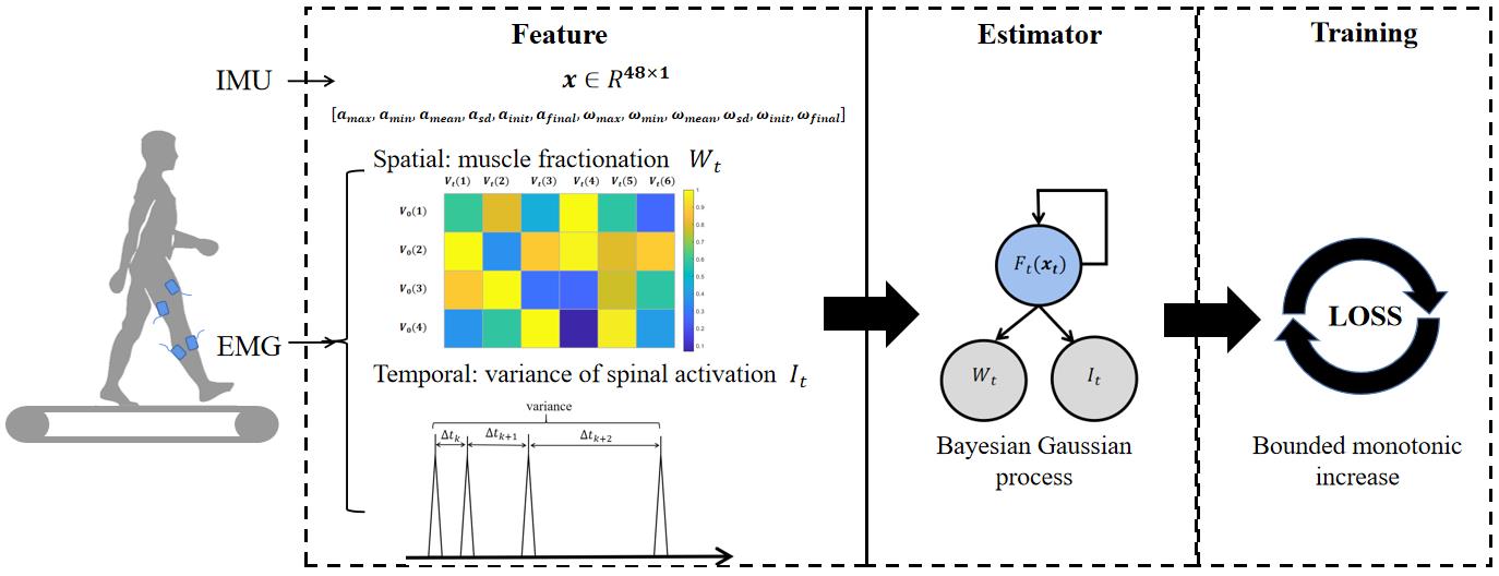
Figure 1: The schematic plot of the workflow. The exercise variable $\bm{x_{t}}$ is extracted from IMU measurements of shank and thigh. The fatigue-induced spatial and temporal patterns of multiple muscles $W_{t}$ and $I_{t}$ are extracted from EMG signals.Then, a directed graph model is built to infer the latent fatigue given the observations, Then, a physiology-inspired loss function is used to train the algorithm.

2.2 Fatigue Assessment

Fatigue is a hidden state of human motor system, which is challenging to measure [7]. Previous works developed various methods to quantify muscle fatigue. Specifically, the biomarker-related methods measure local fatigue-induced adaptations, such as the evoked potential-based methods that measure either cortical or muscle fiber fatigue using stimulation [33], ATP metabolism and oxidative stress-based methods that measure local biochemical changes [34]. Such methods can present biochemical or electrophysiological assessment, but the local measurements are insufficient to reflect the integral fatigue level that is almost whole motor system-involved. That is, either motor cortex or local muscle fiber/metabolite change can hardly reflect the fatigue of walking-like exercise that relates to multi-muscle coordination. Some studies leveraged the decline of motor performance [9, 35] to assess fatigue. For the multi-muscle exercises, non-specific fatigue measuring protocol (e.g. maximum voluntary force of knee extension or rebound jump height) would be inefficient [36] as mentioned above, and the motor parameters of multi-muscle exercise itself would be too high-dimensional to form a unified assessment. For example, the motor performance of walking include over 12 gait parameters [30], which can hardly form a fatigue score. Subjective feelings obtained by self-reported questions although can summarize fatigue as some unified Likert-scale scores, are insufficiently objective nor continuous. Alternative studies proposed data-driven methods that either provide binary fatigue classification [18, 16] or measure the deviation of EMG distributions between a relatively stationary process and the cumulative curve of EMG features [20, 17]. As our comparison below, current data-driven methods can form a unified score, but are limited by their stationary assumptions. Thus, two issues may arise from the lack of gold standard for continuous multi-muscle fatigue. That is, 1) there is no labels to train the proposed fatigue scoring model, and 2) the metrics used to quantitatively evaluate the model would be lacked. In this paper, we train the proposed physiological rationale model by a novel loss function formed by the time-evolving characteristics of fatigue and evaluate the comprehensive muscle fatigue by its almost monotonic increasing trend and its similarities with a self-reported fatigue feelings and EMG distribution changes.

3 Method

In this section, we introduce how we score muscle fatigue of walking through formulating physiological principles of muscle fatigue into a computational model. Specifically, we first summarize the physiological principles and translate them into the prior for the computational model. Second, we design features that can reflect the neural control of multiple muscles as the observation. Third, we develop the physiologically rational model and mathematically formulate the time-evolved dynamics of fatigue. Finally, we form a loss function by the physiological principles of fatigue in order to solve the issue of lacking supervision information.

3.1 The Physiological Prior For The Fatigue Scoring Model

As stated in related work, the progression of muscle fatigue is time-evolved and relates to the task type and training intensity ($P_{1}$). From the perspective of observation, fatigue induces the activation weight change of multiple muscles ($P_{2}$), i.e. muscle compensation, and the supra-spinal inhibition of motor command and a group-level increase of the variance of motoneuron spike timings ($P_{3}$). From the perspective of fatigue dynamics, fatigue presents a weak increasing monotonicity ($P_{4}$). That is, the fatigue score $F_{t}$ generally increases with the increase of training time, but tolerates small jitters in the neighborhood. And the increase of fatigue in the neighbourhood should be bounded. Inspired by such prior, the problem can be formulated as:

$$F_{t}=g(W_{t},I_{t},\bm{x_{t}},F_{t-1})$$ (1)

$$\begin{array}[]{r@{\quad}r@{}l@{\quad}l}s.t.&F_{t}&=\quad F_{t-1}+\delta_{t-1}\\ &|\delta_{t-1}|&\leq\quad\Delta\end{array}$$ (3)

where $t$ denotes the time instant, $W_{t}$ and $I_{t}$ denote the activation weight change of multiple muscles and the spike timing-related changes, respectively, $\bm{x_{t}}$ denotes the exercise variable, $\delta_{t-1}$ and $\Delta$ denote the jitter tolerance and the bounded increase.

3.2 Features of Muscle Compensation And Spinal Adaptations of Spike Timings

In this part, we address the issue of the model input, i.e. the features corresponding to compensation ($P_{2}$) and group-level activation of spinal neurons ($P_{3}$) involved in walking-like multi-muscle coordination. To do so, we use muscle synergy to factorize the multi-muscle signals into spatial patterns to capture muscle compensation and temporal patterns to capture the spinal module activation [37]. Spinal module activation reflects the group-level co-activation of spinal inter-neurons, thus can be used to extract the spike timing adaptations of fatigue. We follow the experience of literature and extract muscle synergies [38, 39] from EMG signals to represent multi-muscle coordination. The measured EMG signals are first band-pass filtered by a zero-phase 6th order Butterworth with cut-off frequencies of 20 and 500 Hz, then rectified to obtain the envelope, then low-pass filtered by a zero-phase 4th order Butterworth with a cut-off frequency of 10Hz and finally used to calculate muscle activation by a recursive filter and an exponential shaping function [40]. Then, we use the non-negative matrix factorization (NMF) to factorize the muscle activation matrix M ($m\times t$, $m$ is the number of muscles and $t$ is the number of samples).

$$M=V\cdot C+e$$ (4)

where $V$ ($m\times n$, $n$ is the number of muscle synergies, also the number of spinal modules) is the muscle weighting components, $C$ ($n\times t$) is the temporal pattern components and $e$ is the residual error matrix. The weight matrix $W$ denotes how multiple muscles coordinate with each other in a spatial manner, each column of which denotes a spatial pattern of muscles corresponded to a muscle synergy. NMF is performed in each sliding window. Herein, we follow the experience of [41] and use the muscle synergy fractionation $Frac_{t}$ to depict the muscle compensation induced by fatigue at each time instant $t$.

$$Frac_{t}(i,k)=\bm{V_{0}}(i)^{T}\cdot\bm{V_{t}}(k)$$ (5)

where $\bm{V_{0}}(i)$ denotes the $i$th column of the initial weight matrix $V_{0}$, $\bm{V_{t}}(k)$ denotes the $k$th column of the latest factorized weight matrix $V_{t}$. We use the similarity between the muscle synergies of the initial sliding window (i.e. original muscle coordination manner) and those of the latest sliding window (i.e. the muscle coordination manner manipulated by fatigue) in order to estimate the merging and fractionation of multi-muscle spatial patterns. Then, we calculate the feature of muscle compensation, $W_{t}$, as the Frobenius norm of $Frac_{t}$. In this way, the muscle compensation of fatigue can be depicted.

Treating the time-varying coefficient matrix $C$ as the smoothed version of spinal module activation [37], we extract the supra-spinal inhibition and the increased group-level variation of spike timings from each row of $C$. Specifically, as presented in our previous work, we first binarize each row of $C$ by its amplitude through K-means. Each binarized sequence denotes the co-activation of the functionally grouped interneurons, i.e. the activation of each spinal module. Then, we pool the binarized sequences into one sequence to denote the activation train of spinal modules. We use $1$ as the spiking of spinal modules and $0$ as de-activation of spinal modules. Finally, we calculate the standard deviation of the interval between each spinal module’s spiking. That is, the standard deviation of the number of $0$ between two nearest $1$ is calculated. In this way, the spinal and group-level activation changes reflected by the variation of spinal module spike timings are depicted. We denote the feature by $I_{t}$.

3.3 The Fatigue Estimator

According to the physiology-inspired problem formulation, the phenomenological view enables us to capture the natural dynamics of fatigue and to model it as a Markov progress. As shown in Fig. 2, we further treat it as a time-evolving directed graph model.

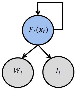
Figure 2: The schematic plot of fatigue dynamic model.

The function $g$ in Eq. (1) serves to update the posterior of fatigue scores given the observations of muscle compensation and spinal module activation variation. To form the posterior updating paradigm, we introduce a latent state $f$ and estimate the muscle fatigue score as follow.

$$F_{t}=\int P(W_{t},I_{t}|f)\cdot p_{t}(f)df$$ (6)

where $p_{t}(f)$ is the posterior of the latent state $f$ at the time instant $t$. It can be obtained recursively in a Bayesian manner, given the exercise variable $\bm{x_{t}}$ and the observations of muscles $W_{t}$ and $I_{t}$.

$$p_{t}(f)=\frac{P(W_{t},I_{t}|f,\bm{x_{t-1}})\cdot p_{t-1}(f|\bm{x_{t-1}})}{\int P(W_{t},I_{t}|f,\bm{x_{t-1}})\cdot p_{t-1}(f|\bm{x_{t-1}})df}$$ (7)

where $W_{t}$ and $I_{t}$ are independent given $f$.

3.3.1 The Prior Capturing The Task Type And Training Intensity

We place a Gaussian prior over the latent state $f$.

$$p_{0}(f)=N(m(\bm{x}),k(\bm{x},\bm{x}^{\prime}))$$ (8)

where $m(\cdot)$ denotes the mean function, $k(\cdot,\cdot)$ denotes the covariance function. We denote $\bm{x_{t}}$ by the IMU features commonly used for classifying gait phases and locomotion modes. The IMU features are cascaded by the traditionally used features extracted from the angular rates and accelerations [42] measured by the two IMUs mounted on shank and thigh, respectively. The dimension of a feature is 48. Herein, we use a linear mean function, $m=\bm{\beta}^{T}\bm{x_{t}}$, where $\bm{\beta}$ is the learnable parameter. And we use the squared exponential kernel to project the exercise variable into a low-dimensional manifold.

$$k(\bm{x},\bm{x}^{\prime}))=exp(-(\bm{x}-\bm{x}^{\prime})^{T}D(\bm{x}-\bm{x}^{\prime}))$$ (9)

where $D$ denotes the diagonal matrix ($48\times 48$) whose diagonal elements $d_{i}$ are the variance of $(\bm{x}-\bm{x}^{\prime})$.

3.3.2 The Likelihood of Observation

In order to form a probit likelihood, we use the cumulative density function of a standard normal $\Phi(y)=\int_{-\infty}^{y}exp(\frac{-x^{2}}{2})dx$. Specifically, the observation likelihood can be formulated as

$$P(W_{t},I_{t}|f,\bm{x_{t}})=\frac{sgm(W_{t})\cdot sgm(I_{t})\cdot(f-m(\bm{(}x_{t})))}{\sigma_{n}^{2}}$$ (10)

where $sgm(\cdot)$ denotes the sigmoid function that squashes the variable inside the bracket into $[0,1]$. Other likelihood functions that present a probit form can also be used.

3.3.3 Posterior Updating Via Gaussian Process Approximation

Directly updating the posterior of the latent function by Eq. 10 is non-Gaussian and hard to have a closed-form solution. In order to iteratively update the posterior, we approximate the posterior $p_{t}(f)$ by the Gaussian distribution that has the smallest Kullback–Leibler (KL) divergence with it. We use the Laplace approximation technique to match the first two moment of the two distributions and can obtain the following update equations.

$$\mu_{t}(\bm{x_{t}}) =\bm{\alpha_{t}^{T}}\bm{k(x_{t})}$$ (11)

$$k_{t}(\bm{x_{t}},\bm{x}^{\prime}) =k(\bm{x_{t}},\bm{x_{t}}^{\prime})+\bm{k(x_{t})}^{T}C_{t}\bm{k(x^{\prime})}$$ (12)

where $\bm{k(x_{t})}=[k(\bm{x_{t-T}},\bm{x_{t}}),...,k(\bm{x_{t-1}},\bm{x_{t}})]$, $\bm{x}^{\prime}=\frac{1}{T}\sum_{i=1}^{T}\bm{x_{t-i}}$, $\bm{\alpha_{t}}$ (a $T$-dimensional vector) and $C_{t}$ ($T\times T$) can be calculated by

$$\bm{\alpha_{t}} =\bm{\alpha_{t-1}}+\gamma_{1}C_{t-1}\bm{k_{t}}$$ (13)

$$C_{t} =C_{t-1}+\gamma_{2}(C_{t-1}\bm{k_{t}})(C_{t-1}\bm{k_{t}})^{T}$$ (14)

where $\bm{k_{t}}=[k(\bm{x_{t-T}},\bm{x_{t-1}}),...,k(\bm{x_{t-1}},\bm{x_{t-1}})]$, $\gamma_{1}$ and $\gamma_{2}$ can be calculated by

$$\gamma_{1} =\partial log\int P(W_{t},I_{t}|f,\bm{x_{t}})df/\partial f$$ (15)

$$\gamma_{2} =\partial^{2}log\int P(W_{t},I_{t}|f,\bm{x_{t}})df/\partial f^{2}$$ (16)

Herein, we set $T$ as 50.

3.3.4 Fatigue Scoring

Given $\bm{\alpha_{t}}$ and $C_{t}$, we can obtain the close-form solutions of the posterior at each time instant, thus can have the fatigue score.

$$F_{t} =\int P(W_{t},I_{t}|f)\cdot p_{t}(f)df$$ (17)

$$=\Phi(\frac{sgm(W_{t})\cdot sgm(I_{t})\cdot(\mu_{t}-m(\bm{x_{t}}))}{\sigma_{x}^{2}})$$ (18)

where $\sigma_{x}=\sqrt{\sigma_{n}^{2}+k(\bm{x_{t}},\bm{x}^{\prime})}$. In this way, we form the fatigue estimator using Bayesian Gaussian Process and can estimate the time-evolving muscle fatigue at each time instant.

3.4 Training

The supervision information for training the model can hardly be obtained. It was reported in [36] that the subjective fatigue feelings and metabolite changes like blood lactic acid can either reflect the global inner feeling or the biochemical body fluid changes of local muscles. Neither of them is a biased measurement of nervous system adaptation induced by muscle fatigue, especially for multi-muscle coordinated exercises, and can not be treated equally. Moreover, both the subjective feelings and the metabolite changes are measured discretely in each time section. That is, neither the time resolution nor the measurement method of them can contribute to a continuous measurement. Thus, we turn to formulating the loss function using the principles of the fatigue itself. The development of fatigue during exercise follows the following rules.

• Fatigue increases as the exercise goes on.

• The muscle fatigue should increase gradually. That is, the increase in the neighborhood should be bounded.

The loss function can thus be formulated as

$$L=\sum_{p}(\Delta(F_{p_{1}},F_{p_{2}})+(1-F_{p_{1}})^{2}+(1-F_{p_{2}})^{2})$$ (19)

$$\Delta(F_{p_{1}},F_{p_{2}})=ReLu(( (F_{p_{1}}-F_{p_{2}}-(p_{1}-p_{2})\cdot\delta)^{2})$$

$$-((p_{1}-p_{2})\cdot\delta)^{2})$$

where $p$ denotes the $p$th pair of time instants $(p_{1},p_{2}),p_{1}>p_{2}$, $F_{p_{i}},i=1,2$ denotes the fatigue score at the $p_{i}$th time instant, $\Delta(F_{p_{1}},F_{p_{2}})$ denotes the weak monotonicity that tolerates jitters if $p_{1}$ is close to $p_{2}$. As shown in Fig. 3, $\Delta(x)=ReLu((x-\delta)^{2}-\delta^{2})$ can tolerate the increase bounded by $2\delta$. In Eg.(19), the bound is further scaled by the time distance of the index pair $(p_{1},p_{2})$. With the loss function, we train the learnable parameters $\bm{\beta}$ and $D$ that are shared among subjects in an end-to-end manner. Specifically, we generate data pairs corresponded to the index pair $(p_{1},p_{2})$ in the training set and the validation set. The Adam optimizer is used. And the learning rate is set as 0.1. The algorithm is trained with the Adam optimizer, the learning rate of 0.1 and the batch size of 100 pairs. The training stops when the decrease of loss between epochs is lower than 0.001 for over 3 times or the maximum 1000 epochs are reached or early stopping criteria is reached on the validation set. We split the whole data set into training, validation and test set following a 7:1:2 strategy. For each epoch, $\bm{\alpha_{t}}$ and $C_{t}$ are initialized as a vector whose elements are randomly set in the range of $(0,0.2)$ and a diagonal matrix whose diagonal elements are randomly set in the range of $(0,2)$. During the testing phase, we randomly initialize $\bm{\alpha_{t}}$ and $C_{t}$ using the same strategy 100 times in order to average the effects of the initialization. All the data are processed by MATLAB 2015b.

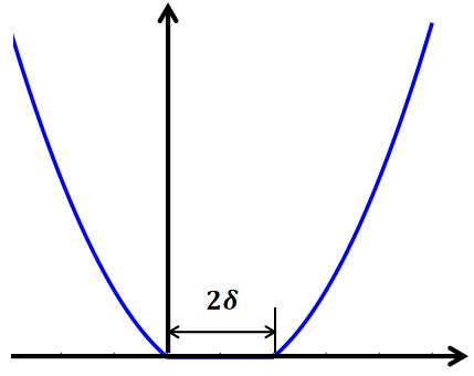
Figure 3: The schematic plot of $y=\Delta(x)$.

4 Evaluation

We take an initial step toward continuously assessing muscle fatigue under the scenario of sub-maximal and dynamic contractions of multi-muscles. In this section, we evaluate the proposed method by testing its cross-day stability, similarities with other measurements of fatigue (e.g. EMG data distribution, subjective feelings) and similarities among subjects. To do so, we first introduce the data collection paradigm and the metrics we use to evaluate the performance. Then, we compare with representative algorithms using the data set and metrics. Under such evaluations, we aim to examine whether the muscle fatigue assessed by our method is stable under different days, and can reflect the common principles among subjects and measurements.

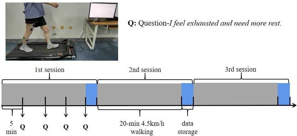
Figure 4: The schematic plot of the experimental paradigm.

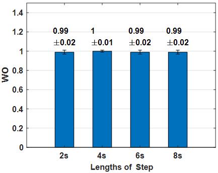
(a) $WO$

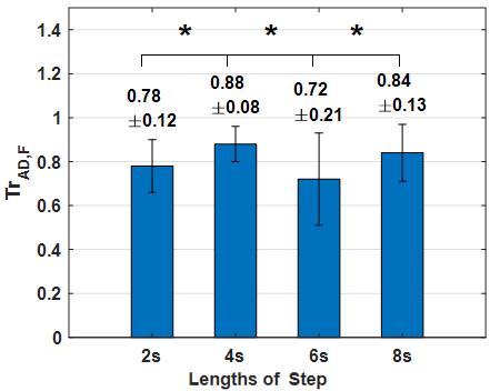
(b) $Tr_{AD,F}$

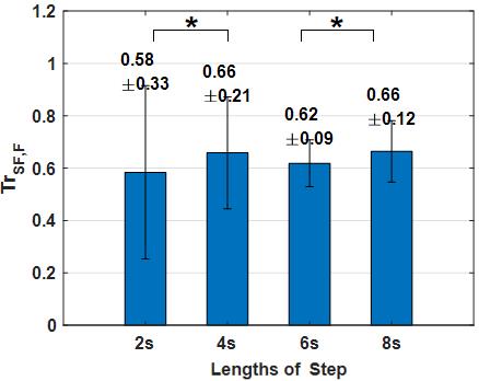
(c) $Tr_{SF,F}$

Figure 5: The performance of different lengths of steps. $*$ indicates a statistically significant difference with other conditions (paired t-test, $\alpha<$0.05).

4.1 Data Collection

Ten subjects (5 males and 5 females, age range: 18-45 years old, weight range: 45-100 kg) were recruited and asked to walk at the speed of 4.5km/h on a treadmill for three sessions. As shown in Fig. 4, each session consists of a 20-minute walking. Every 5 minutes, the subjects were asked to report their physical fatigue feelings using a 7-point Likert scale in response to the question: I feel exhausted and need more rest. The left-most point corresponded to “Strongly Agree” and the right-most point corresponded to “Strongly Disagree”. Sitting down was not allowed between sessions, and the time between sessions was for the data storage purpose and lasted for maximum 2minutes. We conducted the same experiment at a separate day. Two of the ten subjects came back 2 days later. Three of the ten subjects came back 3 days later. One subject came back 5 days later. The rest of them came back a week later. We do not constrain the same placement of EMG sensors on separate days. Each subject signed the informed consent before the experiment and the experimental protocol was approved by Chinese Ethics Committee of Registering Clinical Trials (ChiECRCT20200319).

Bipolar EMG sensors (Trigno Wireless System; DELSYS, Boston, MA, USA) were placed on the surface of target muscles after skin preparation through palpation. The 9 muscles are rectus femoris (RF), vastus lateralis (VL),vastus medialis (VM), tibialis anterior(TA), soleus(SOL), semitendinosus(ST), biceps femoris (long head ,BF), gastrocnemius lateralis(LG), gastrocnemius medialis (MG). The sampling rate of EMG signals was 1111.11 Hz. Foot pressure sensors were attached to the heel and first metatarsal bone of the subject for phase labeling (swing phase, initial contact, midstance and propulsion), with the sampling rate of 500 Hz. The two signals were synchronized by a trigger device.

4.2 Metrics

(a) $WO$

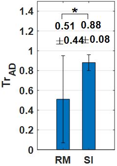
(b) $Tr_{AD}$

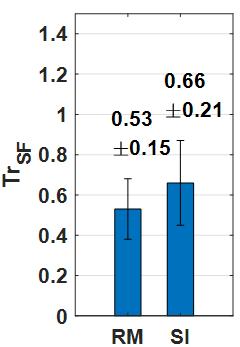
(c) $Tr_{SF}$

Figure 6: The performance of different input features. $*$ indicates a statistically significant difference (paired t-test, $\alpha<$0.05).

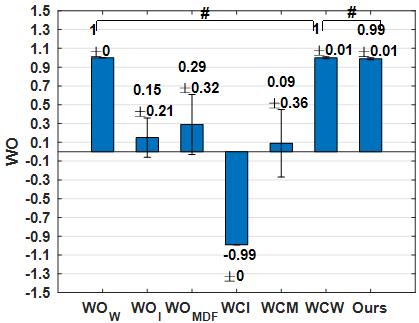
(a) $WO$

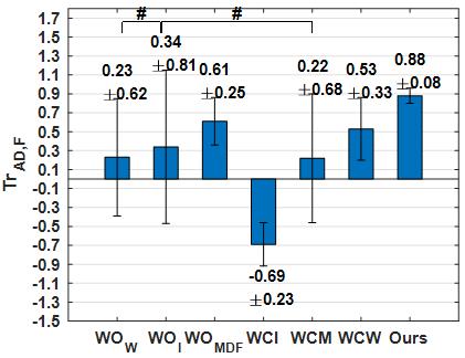
(b) $Tr_{AD,F}$

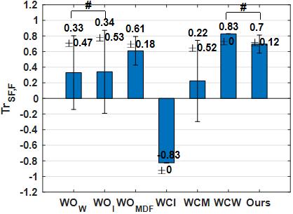
(c) $Tr_{SF,F}$

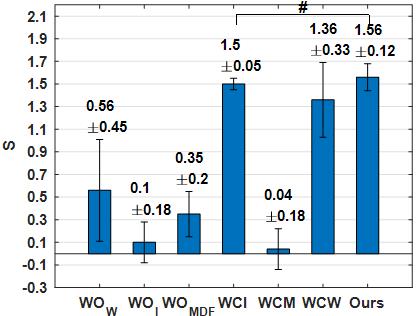
(d) $S$

Figure 7: The performance comparison of different methods. $\#$ indicates there is no statistically significant difference (paired t-test, $\alpha\geq$ 0.05).

Currently developed methods evaluate the assessed muscle fatigue either by the detection accuracies for the binary classification task or by the degradation of motor performance (e.g. the maximum muscle force) for isometric contractions. Some studies just focused on the principles presented by their proposed method [15, 21], without quantitatively evaluating the performance. Considering there is no gold standard to assess muscle fatigue for walking, we evaluate the performance by the metrics of the common rules that muscle fatigue should follow. Herein, we adopt the metrics proposed by [22] for evaluating rehabilitation progress and feature selection of multiple biomedical usages [17].

4.2.1 Weak Monotonicity (WO)

For a continuous fatigue score $J_{j}$, we first calculate how many sample points of the score trajectory fall into the range of weakly monotonic increasing. The tolerance for the weak monotonicity is set as delta. The points that follow the weak monotonicity consist of $D_{j}^{+}$ and the other points consist of $D_{j}^{-}$.

$$D_{j}^{+} =\{J_{j}(t)|J_{j}(t)>J_{j}(t-1)+\delta_{j}(t-1)\}$$ (20)

$$D_{j}^{-} =\{J_{j}(t)|J_{j}(t)\notin D^{+}\}$$

where $\delta_{j}$ should accommodate the variation of the trajectory $J_{j}$, thus can be calculated as the standard deviation of the trajectory, i.e. $\delta_{j}=std(J_{j})$. We further calculate the number of points in $D_{j}^{+}$ and $D_{j}^{+}$ as $Num^{+}$ and $Num^{-}$, respectively. Then, we calculate WO by

$$WO_{j}=\frac{Num^{+}}{N-1}-\frac{Num^{-}}{N-1}$$ (21)

where $N$ denotes the total number of the sample points of the trajectory.

4.2.2 Trendability (Tr)

It is assumed that different measurements of fatigue, although present different views and perspectives, should follow some common trends. In addition, common trends should also exist among subjects and among different days. The trendability can be calculated as the similarity between two trajectories. We evaluate the trendability by

$$Tr=Corr(J_{1},J_{2})$$ (22)

where $Corr(\cdot)$ denotes the Pearson coefficient.

4.2.3 Suitability (S)

Suitability combines weak monotonicity and trendability to evaluate the fatigue score comprehensively.

$$S=(WO_{1}+WO_{2})\cdot Tr$$ (23)

4.3 Lengths of The Sliding Window

We extract features from each sliding window and use it to estimate the fatigue score. Considering NMF’s requirement of data quantity and the time sensitivity of fatigue [15, 21], we limit the minimum length of window as 2 seconds and we set the step length the same as the window length. We perform grid search and evaluate the performance by 1) calculating the $WO$s of each window length and 2) calculating the estimated fatigue score’s similarity with the subjective feelings and with the EMG-based gait phase classification accuracy. Specifically, we down-sample or B-spline interpolate the estimated fatigue score to match the time instants of subjective feelings (SF). Then, we use $Tr_{SF,F}$ to evaluate the similarity between each subject’s SF and F. To obtain the gait phase classification accuracy, we extract the classic feature set, Hudgin’s set [43], with the recommended window length of 128 ms and step of 15ms. We train the classifier with the first 2-minute data and test its accuracy using the data in the following time. And we calculate the accuracy degradation (AD). Similarly, we use $Tr_{AD,F}$ to evaluate the similarity between the two trajectories. With the common trend among AD, SF and F, we evaluate to what extent the estimated fatigue score $F_{t}$ follows the trend of subjective feelings and the data distribution changes. The metrics are averaged over subjects and days. Paired t-tests are used to test the significant difference. And the Shapiro-Wilk test is performed to test normality. Alpha level is set as 0.05.

As shown in Fig.5, WO does not present a significant difference among steps, while $Tr_{AD,F}$ and $Tr{{}_{S}F,F}$ present significant but small differences. It can be shown that the step of 4 seconds and 8 seconds present almost the same and better than other steps. Considering the time resolution of the method, we choose 4 seconds as the final step length.

4.4 Influence of Input Features

We test the influence of different features. Following the experience of using the root mean square (RMS) and the median frequency (MDF) to depict fatigue, we perform PCA on the RMS and MDF of the 9 muscles and extract the first principle components denoted by $P_{RMS}$ and $P_{MDF}$, respectively. $P_{RMS}$ and $P_{MDF}$ are used as the inputs for the estimator to replace $W_{t}$ and $I_{t}$. We use $WO_{RM}$ and $WO_{SI}$ for the weak monotonicity comparison and use $Tr_{AD,F}$ and $Tr_{SF,F}$ versus $Tr_{AD,RM}$ and $Tr_{SF,RM}$ for the trendability comparison. The performance is averaged over subjects and days. Alpha level is set as 0.05.

It can be seen from Fig. 7 that our proposed features $W_{t}$ and $I_{t}$ generally outperform the features RMS and MDF traditionally used for estimating muscle fatigue under isometric or static contractions. The results indicate solely depicting single muscle properties for multi-muscle contractions could be insufficient.

4.5 Fatigue Assessment

We herein compare our proposed method with the methods that also use EMG signals to continuously assess muscle fatigue. We adopt the weighted-cumulative fatigue estimator (WCF) [20] that utilizes the static and Markov assumptions of fatigue. Other than $W_{t}$ and $I_{t}$, we use the demonstrated input MDF and apply PCA on the muscles to obtain the first principle component. Following [20], we use the discrepancy between the WCF and the static Markov process as the fatigue score. In addition, we also use the WO-based method to translate features into WO scores for depicting muscle fatigue. Following the idea of [17], we use the ratio of the points in a sliding window that do not follow the weak monotonicity principle as the metrics of fatigue. We also use the first principle component of MDF, $W_{t}$ and $I_{t}$ as the input features. For a fair comparison purpose, the same windowing scheme is used. We perform the comparison by presenting WO, $Tr_{AD,F}$ and $Tr_{SF,F}$ of each estimated fatigue score. Moreover, we provide a comprehensive evaluation by calculating the suitability (S) using WO and the averaged Tr. The performance is averaged over subjects and days. Alpha level is set as 0.05.

As shown in Fig. 7, our method presents similarly good weak mononitivity with $WO_{W}$ and $WCW$, but outperform them by $Tr_{AD,F}$ and the overall metric $S$. It can be shown in Fig. 7 that although $WCW$ presents a larger $Tr_{SF,F}$, there is no significance between $WCW$ and our method. $WCI$ presents negative WO and trendabilities, which indicates the potentially poor performance for continuously assessing muscle fatigue. Similarly, $WCI$ presents a relatively large suitability, but suffers from small or even negative WO and Tr. $WO_{W}$, $WO_{I}$, $WO_{MDF}$, $WCM$ present relatively small values of trendabilities and suitabilities, which also indicate their worsened performance when applyed on the multi-muscle coordinated exercise.

4.6 Cross-Day Stability

We test the cross-day stability by presenting the two separate days’ trendability ($Tr_{D1,D2}$) and suitability ($S_{D1,D2}$). We present the cross-day performance of the above-mentioned methods.

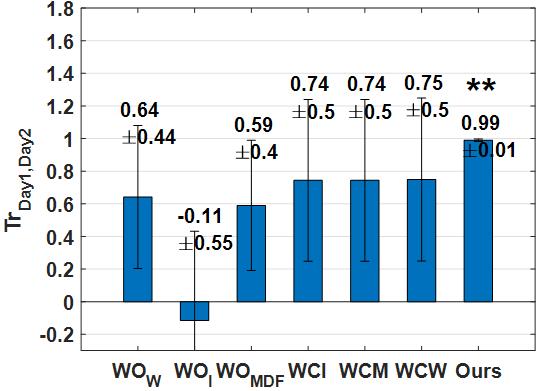
(a) $Tr_{D1,D2}$

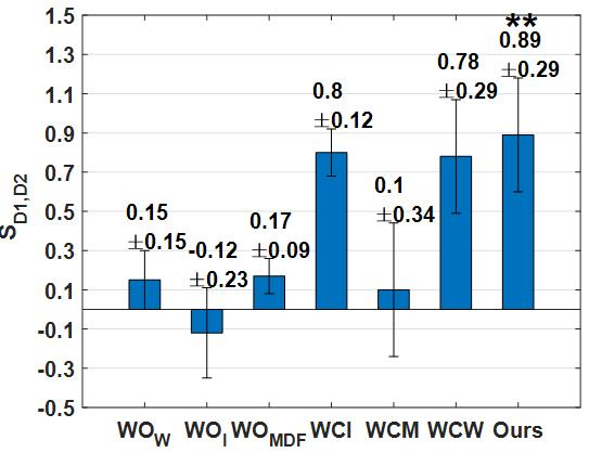
(b) $S_{D1,D2}$

Figure 8: The performance of different days. $**$ indicates a statistically significant difference with other conditions (paired t-test, $\alpha<$0.05).

As shown in Fig. 8, the weighted cumulative estimator-based methods ($WCI$, $WCM$, $WCW$) present a relatively stable performance under the cross-day scenario. This meets the performance demonstrated in [20] under isometric contractions. For the sub-maximal and dynamic contractions of multiple muscles, our method outperforms the weighted cumulative estimator-based methods by the trendabilities and suitabilities between days. In addition, the weak monotonicity-based methods ($WO_{W}$, $WO_{I}$, $WO_{MDF}$) present worsened performance, which indicates their insufficient stability for cross-day measurements.

4.7 Cross-Subject and Cross-View Similarities

We present whether the fatigue progressing trend is common among subjects and among different views of fatigue (i.e. subjective feelings, data distribution changes and fatigue scores). Through evaluating the cross-subject similarity, we aim to further test the feasibility of our method and more importantly provide a cue for further researches that fatigue might be evolved following a common principle. Herein, we present the representative plot of each view of fatigue and Tr of each pair of subjects averaged over days.

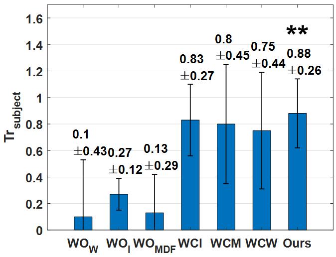
Figure 9: The trendability among subjects and averaged over subject pairs. $**$ indicates a statistically significant difference with other conditions (paired t-test, $\alpha<$0.05).

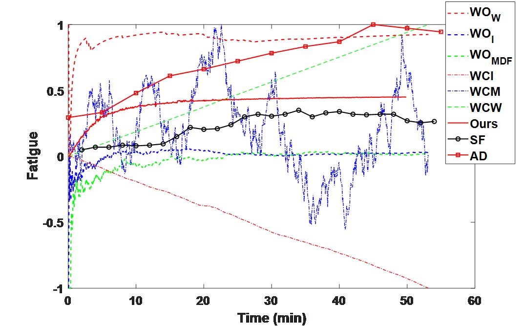
Figure 10: The representative examples of different views of fatigue. All the metrics except for $Ours$ and $AD$ are normalized by their maximum. $AD$ is normalized by 100 to denote the percents.

As shown in Fig. 9, our method significantly outperforms other methods by the cross-subject similarities. The progression of fatigue share some common trends among subjects, despite individual characteristics. For example, at least a monotonic increase of the estimated fatigue should be shared among subjects. In addition, as shown in Fig. 10, different estimates of fatigue (WO-based methods, weighted cumulative estimator-based methods and our method) present different trends. Although we do not know the gold standard of fatigue, at least a negative estimate, unbounded estimate or a saturated estimate shall not be the top candidate for depicting and assessing muscle fatigue. Moreover, AD, SF, $WO_{W}$, $WCM$, $WCW$ and $Ours$ present similarly increasing trends.

5 Discussion

In this study, we propose to depict the continuous progression of muscle fatigue under multi-muscle coordinated exercise and formulate the issue into a rationale model that takes physiological priors into account. We then solve the issue of lacking metrics to evaluate the fatigue estimator’s performance by adopting the metrics of weak monotonicity, trendability and suitability. Through extensive experiments, we evaluate our method’s performance of different hyper-parameters and input features, and the cross-day stability, cross-subject and cross-view similarities. We also compare our method with state-of-the-art methods. The results demonstrate our method’s considerable stability and coincidence with the principles of fatigue progression.

Feasibility of the input features. RMS and MDF are traditionally used EMG features to depict fatigue, which have been demonstrated with similar characteristics with the local muscle changes of myofiber mechanical oscillations and muscular oxygen metabolism [15]. The feature comparison demonstrates the multi-muscle properties can better depict the fatigue characteristics of walking than single muscle properties. This further indicates the muscle spatial coordination and temporal group-level neuronal activities can better reflect the fatigue-induced motor-level adaptations of complex muscle coordination, like walking.

Weak monotonicity, trendability and suitability of fatigue. It is common sense that as the exercise continues, the muscle fatigue accumulates and the score or the degree of fatigue should increase. And the experimental results of fatigue [44, 33] that reveals the fatigue-induced changes of central motor regions, motor output and motor units also implicitly demonstrate the common sense and present a common trend. Moreover, the estimated fatigue score’s similarities with other views of fatigue, i.e. $Tr_{SF,F}$ and $Tr_{AD,F}$, provide further demonstrations of to what extent the estimated fatigue score follow the common trend of fatigue progression, given there is no gold standard for objective muscle fatigue, especially for multi-muscle exercise. Our comparison demonstrates the overall best performance of our method compared with the SOTA methods that can continuously assess muscle fatigue. It can be seen that our method presents similar $WO$, $Tr_{SF,F}$ compared with $WO_{W}$ and $WCM$, and significantly better $Tr_{AD,F}$ compared with $WCM$. Also, it can be seen from Fig. 10 that other than the worse trendability of $WCM$, all the weighted cumulative estimator-based methods present a nearly unbounded and constant-speed increase of muscle fatigue, which could violate the objective principle of fatigue progression revealed by multiple views. The best suitability S further demonstrates the overall performance of our method.

Cross-day stability. The reason of our method’s best stability presented in our comparison can be twofold. First, the physiological rationale features extract latent states of neuro-muscular control of multi-muscle coordination [38], and have been demonstrated with good stability [37]. This can also be demonstrated by $WCM$’s and $WCI$’s better suitability compared with $WCM$, $WO_{W}$, $WO_{I}$ and $WO_{MDF}$, shown in Fig. Second, the proposed estimator is rationally modeled and trained by the fatigue progression-inspired loss function, thus can extract more fatigue-related information. This can be demonstrated by the better performance of our method compared with all the other SOTA estimators. even though input features can the same.

Cross-subject and cross-view similarities. Previous studies usually present discrete measurements of fatigue-related indices to indicate the fatigue-induced adaptations. Our proposed method provides a general measurement for multi-muscle exercise with good cross-subject similarities, compared with SOTA methods. Moreover, fatigue studies use muscle metabolism, muscle activation patterns, motor region activities etc. to investigate the changes of specific regions under peripheral or central fatigue. The cross-subject and cross-view similarities among the estimated muscle fatigue score, subjective fatigue feelings and the fatigue-induced shift of EMG data distribution indicate there might be a latent bodily state that regulates the fatigue-related aspects, no matter biomechanics, inner feelings or neural systems, as suggested by theoretical frameworks [45, 36]. It should be noted that the fatigue-related bodily state regulation is out of the scope. We herein just propose a cue for future research.

Limitations and future work. This study is just a proof-of-concept work that has several limitations. First, the study does not consider the condition of taking rest. When there is a rest session between two exercise sessions, the monotonically increasing trend of fatigue would be violated. And the whole fatigue progression would be piece-wise monotonic. Second, more exercise modalities should be included. For example, if there is a running session after walking sessions, the increasing rate of fatigue would change and the bound of fatigue score would also break. And further running-related physiological priors can be included. Third, the model we develop utilizes the Markov, Gaussian and Bayesian assumptions. The actual fatigue progression might violate such assumptions. Future work should also develop models beyond the assumptions.

6 Conclusion

This study takes the first step toward conceptualizing and continuously assessing objective muscle fatigue for daily exercise. The proposed method utilizes the features of spatial and temporal adaptations of multi-muscle coordination and group-level neuronal activities. The fatigue can then be continuously estimated using a physiological rationale model built by a Bayesian Gaussian process, and trained by a time-evolving principle-inspired loss function. The experimental results demonstrate the cross-day stability, coincidence with fatigue progressions and other views of fatigue and our method’s benefits over other methods. Furthermore, our results indicate the existence of a bodily state that regulates fatigue and provides a cue for further research. The promising outcomes of our study may aid fatigue monitoring, training endorsement determination and human-machine interface for more exercise modalities.

References

- [1] R. M. Enoka and J. Duchateau, “Muscle fatigue: what, why and how it influences muscle function,” The Journal of physiology, vol. 586, no. 1, pp. 11–23, 2008.
- [2] S.-H. Liu, C.-B. Lin, Y. Chen et al., “An emg patch for the real-time monitoring of muscle-fatigue conditions during exercise,” Sensors, vol. 19, no. 14, p. 3108, 2019.
- [3] M. Gruet, “Fatigue in chronic respiratory diseases: theoretical framework and implications for real-life performance and rehabilitation,” Frontiers in Physiology, vol. 9, p. 1285, 2018.
- [4] L. Peternel, C. Fang, N. Tsagarakis, and A. Ajoudani, “A selective muscle fatigue management approach to ergonomic human-robot co-manipulation,” Robotics and Computer-Integrated Manufacturing, vol. 58, pp. 69–79, 2019.
- [5] G. Liang, X. Li, Y. Wang, S. Yang, Z. Huang, Q. Yang, D. Wang, B. Dong, M. Zhu, and C. Zhi, “Building durable aqueous k-ion capacitors based on mxene family,” Nano Research Energy, vol. 1, no. 1, p. e9120002, 2022.
- [6] J. R. Yancey and S. M. Thomas, “Chronic fatigue syndrome: diagnosis and treatment,” American family physician, vol. 86, no. 8, pp. 741–746, 2012.
- [7] G. Marco, B. Alberto, and V. Taian, “Surface emg and muscle fatigue: multi-channel approaches to the study of myoelectric manifestations of muscle fatigue,” Physiological measurement, vol. 38, no. 5, p. R27, 2017.
- [8] G. Zhang, E. Morin, Y. Zhang, and S. A. Etemad, “Non-invasive detection of low-level muscle fatigue using surface emg with wavelet decomposition,” in 2018 40th Annual International Conference of the IEEE Engineering in Medicine and Biology Society (EMBC). IEEE, 2018, pp. 5648–5651.
- [9] M. Mugnosso, F. Marini, M. Holmes et al., “Muscle fatigue assessment during robot-mediated movements,” Journal of neuroengineering and rehabilitation, vol. 15, no. 1, pp. 1–14, 2018.
- [10] S. Wang, H. Tang, B. Wang, and J. Mo, “A novel approach to detecting muscle fatigue based on semg by using neural architecture search framework,” IEEE Transactions on Neural Networks and Learning Systems, 2021.
- [11] A. Fidalgo-Herrera, J. Miangolarra-Page, and M. Carratalá-Tejada, “Electromyographic traces of motor unit synchronization of fatigued lower limb muscles during gait,” Human Movement Science, vol. 75, p. 102750, 2021.
- [12] J. Taelman, J. Vanderhaegen, M. Robijns et al., “Estimation of muscle fatigue using surface electromyography and near-infrared spectroscopy,” in Oxygen Transport to Tissue XXXII. Springer, 2011, pp. 353–359.
- [13] E. Cè, S. Rampichini, E. Monti et al., “Changes in the electromechanical delay components during a fatiguing stimulation in human skeletal muscle: an emg, mmg and force combined approach,” European journal of applied physiology, vol. 117, no. 1, pp. 95–107, 2017.
- [14] J. P. V. Anders, C. M. Smith, J. L. Keller et al., “Inter-and intra-individual differences in emg and mmg during maximal, bilateral, dynamic leg extensions,” Sports, vol. 7, no. 7, p. 175, 2019.
- [15] W. Guo, X. Sheng, and X. Zhu, “Assessment of muscle fatigue based on motor unit firing, muscular vibration and oxygenation via hybrid mini-grid semg, mmg, and nirs sensing,” IEEE Transactions on Instrumentation and Measurement, vol. 71, pp. 1–10, 2022.
- [16] A. Moniri, D. Terracina, J. Rodriguez-Manzano et al., “Real-time forecasting of semg features for trunk muscle fatigue using machine learning,” IEEE Transactions on Biomedical Engineering, vol. 68, no. 2, pp. 718–727, 2020.
- [17] X. Guo, L. Lu, M. Robinson et al., “A weak monotonicity based muscle fatigue detection algorithm for a short-duration poor posture using semg measurements,” in 2021 43rd Annual International Conference of the IEEE Engineering in Medicine & Biology Society (EMBC). IEEE, 2021, pp. 2238–2241.
- [18] Y. Jiang, V. Hernandez, G. Venture et al., “A data-driven approach to predict fatigue in exercise based on motion data from wearable sensors or force plate,” Sensors, vol. 21, no. 4, p. 1499, 2021.
- [19] L. Xu, X. Chen, S. Cao et al., “A fatigue involved modification framework for force estimation in fatiguing contraction,” IEEE Transactions on Neural Systems and Rehabilitation Engineering, vol. 26, no. 11, pp. 2153–2164, 2018.
- [20] V. d. A. Rocha, J. C. do Carmo, and F. A. d. O. Nascimento, “Weighted-cumulated s-emg muscle fatigue estimator,” IEEE Journal of Biomedical and Health Informatics, vol. 22, no. 6, pp. 1854–1862, 2017.
- [21] F. A. de Oliveira Nascimento, V. de Araújo Rocha, and J. C. do Carmo, “Scalable weighted-cumulated methodology for fatigue estimation,” Research on Biomedical Engineering, pp. 1–15, 2022.
- [22] L. Lu, Y. Tan, M. Klaic et al., “Evaluating rehabilitation progress using motion features identified by machine learning,” IEEE Transactions on Biomedical Engineering, vol. 68, no. 4, pp. 1417–1428, 2020.
- [23] J. L. Taylor, M. Amann, J. Duchateau et al., “Neural contributions to muscle fatigue: from the brain to the muscle and back again,” Medicine and science in sports and exercise, vol. 48, no. 11, p. 2294, 2016.
- [24] J. L. Taylor and S. C. Gandevia, “A comparison of central aspects of fatigue in submaximal and maximal voluntary contractions,” Journal of applied physiology, vol. 104, no. 2, pp. 542–550, 2008.
- [25] K. Thomas, S. Goodall, M. Stone et al., “Central and peripheral fatigue in male cyclists after 4-, 20-, and 40-km time trials,” Medicine & Science in Sports & Exercise, vol. 47, no. 3, pp. 537–546, 2015.
- [26] P. Edouard, J. Mendiguchia, J. Lahti et al., “Sprint acceleration mechanics in fatigue conditions: compensatory role of gluteal muscles in horizontal force production and potential protection of hamstring muscles,” Frontiers in physiology, vol. 9, p. 1706, 2018.
- [27] U. Granacher, I. Wolf, A. Wehrle et al., “Effects of muscle fatigue on gait characteristics under single and dual-task conditions in young and older adults,” Journal of neuroengineering and rehabilitation, vol. 7, no. 1, pp. 1–12, 2010.
- [28] F. A. Barbieri, P. C. R. dos Santos et al., “Interactions of age and leg muscle fatigue on unobstructed walking and obstacle crossing,” Gait & posture, vol. 39, no. 3, pp. 985–990, 2014.
- [29] S. Morrison, S. R. Colberg, H. K. Parson et al., “Walking-induced fatigue leads to increased falls risk in older adults,” Journal of the American Medical Directors Association, vol. 17, no. 5, pp. 402–409, 2016.
- [30] P. C. R. dos Santos, “Effects of age and fatigue on human gait,” Ph.D. dissertation, University of Groningen, 2020.
- [31] X. Xi, S. Pi, Y.-B. Zhao et al., “Effect of muscle fatigue on the cortical-muscle network: a combined electroencephalogram and electromyogram study,” Brain Research, vol. 1752, p. 147221, 2021.
- [32] X. Liu, M. Zhou, Y. Geng et al., “Changes in synchronization of the motor unit in muscle fatigue condition during the dynamic and isometric contraction in the biceps brachii muscle,” Neuroscience Letters, vol. 761, p. 136101, 2021.
- [33] M. Gruet, J. Temesi, T. Rupp et al., “Stimulation of the motor cortex and corticospinal tract to assess human muscle fatigue,” Neuroscience, vol. 231, pp. 384–399, 2013.
- [34] A. J. Siegel, J. Januzzi, P. Sluss, E. Lee-Lewandrowski, M. Wood, T. Shirey, and K. B. Lewandrowski, “Cardiac biomarkers, electrolytes, and other analytes in collapsed marathon runners: implications for the evaluation of runners following competition,” American journal of clinical pathology, vol. 129, no. 6, pp. 948–951, 2008.
- [35] L. Sanchez-Medina and J. J. González-Badillo, “Velocity loss as an indicator of neuromuscular fatigue during resistance training.” Medicine and science in sports and exercise, vol. 43, no. 9, pp. 1725–1734, 2011.
- [36] J. C. Weavil and M. Amann, “Neuromuscular fatigue during whole body exercise,” Current opinion in physiology, vol. 10, pp. 128–136, 2019.
- [37] C. Yi, F. Jiang, G. Lu et al., “A bipolar myoelectric sensor-enabled human-machine interface based on spinal module activations,” in 2021 IEEE International Conference on Robotics and Automation (ICRA). IEEE, 2021, pp. 1269–1275.
- [38] S. A. Chvatal and L. H. Ting, “Common muscle synergies for balance and walking,” Frontiers in computational neuroscience, vol. 7, p. 48, 2013.
- [39] P. Kieliba, P. Tropea, E. Pirondini et al., “How are muscle synergies affected by electromyography pre-processing?” IEEE transactions on neural systems and rehabilitation engineering, vol. 26, no. 4, pp. 882–893, 2018.
- [40] J. Potvin, R. Norman, and S. McGill, “Mechanically corrected emg for the continuous estimation of erector spinae muscle loading during repetitive lifting,” European journal of applied physiology and occupational physiology, vol. 74, no. 1, pp. 119–132, 1996.
- [41] V. C. Cheung, B. M. Cheung, J. H. Zhang et al., “Plasticity of muscle synergies through fractionation and merging during development and training of human runners,” Nature communications, vol. 11, no. 1, pp. 1–15, 2020.
- [42] B. Barshan and M. C. Yüksek, “Recognizing daily and sports activities in two open source machine learning environments using body-worn sensor units,” The Computer Journal, vol. 57, no. 11, pp. 1649–1667, 2014.
- [43] K. Englehart and B. Hudgins, “A robust, real-time control scheme for multifunction myoelectric control,” IEEE transactions on biomedical engineering, vol. 50, no. 7, pp. 848–854, 2003.
- [44] P. Sarker and G. A. Mirka, “The effects of repetitive bouts of a fatiguing exertion (with breaks) on the slope of emg measures of localized muscle fatigue,” Journal of Electromyography and Kinesiology, vol. 51, p. 102382, 2020.
- [45] T. J. Hureau, L. M. Romer, and M. Amann, “The ‘sensory tolerance limit’: A hypothetical construct determining exercise performance?” European journal of sport science, vol. 18, no. 1, pp. 13–24, 2018.