NeRF-Supervised Deep Stereo

Abstract

We introduce a novel framework for training deep stereo networks effortlessly and without any ground-truth. By leveraging state-of-the-art neural rendering solutions, we generate stereo training data from image sequences collected with a single handheld camera. On top of them, a NeRF-supervised training procedure is carried out, from which we exploit rendered stereo triplets to compensate for occlusions and depth maps as proxy labels. This results in stereo networks capable of predicting sharp and detailed disparity maps. Experimental results show that models trained under this regime yield a 30-40% improvement over existing self-supervised methods on the challenging Middlebury dataset, filling the gap to supervised models and, most times, outperforming them at zero-shot generalization.

Fig. 1. Zero-Shot Generalization Results. On top, predictions by RAFT-Stereo [35] trained with our approach on user-collected images, without using any synthetic datasets, ground-truth depth or (even) real stereo pairs. At the bottom, a zoom-in over the Backpack disparity map, showing an unprecedented level of detail compared to existing strategies not using ground-truth [79, 3, 23] trained with the same data.

1 Introduction

Depth from stereo is one of the longest-standing research fields in computer vision [38]. It involves finding pixels correspondences across two rectified images to obtain the disparity – i.e., their difference in terms of horizontal coordinates – and then use it to triangulate depth. After years of studies with hand-crafted algorithms [56], deep learning radically changed the way of approaching the problem [74]. End-to-end deep networks [50] rapidly became the dominant solution for stereo, delivering outstanding results on benchmarks [42, 55, 58] given sufficient training data.

This latter requirement is the key factor for their success, but it is also one of the greatest limitations. Annotated data is hard to source when dealing with depth estimation since additional sensors are required (e.g., LiDARs), and thus represents a thick entry barrier to the field. Over the years, two main trends have allowed to soften this problem: self-supervised learning paradigms [23, 76, 3] and the use of synthetic data [41, 75, 30]. Despite these advances, both approaches still have weaknesses to address.

Self-supervised learning: despite the possibility to train on any unlabeled stereo pair collected by any user – and potentially opening to data democratization – the use of self-supervised losses is ineffective at dealing with ill-posed stereo settings (e.g. occlusions, non-Lambertian surfaces, etc.). Albeit recent approaches soften the occlusions problem [3], predictions are far from being as sharp, detailed and accurate as those obtained through supervised training. Moreover, the self-supervised stereo literature [76, 29, 13] often focuses on well-defined domains (i.e., KITTI) and rarely exposes domain generalization capabilities [3].

Synthetic data: although training on densely annotated synthetic images can guide the networks towards sharp, detailed and accurate predictions, the domain-shift that occurs when testing on real data dampens the full potential of the trained model. A large body of recent literature addressing zero-shot generalization [2, 35, 30, 36, 16, 87] proves how relevant the problem is. However, obtaining stereo pairs as realistic as possible requires significant effort, despite synthetic depth labels being easily sourced through a graphics rendering pipeline. Indeed, modelling high-quality assets is crucial for mitigating the domain shift and requires excellent graphics skills. While artists make various assets available, these are seldom open source and necessitate additional human labor to be organized into plausible scenes.

In short, in a world where data is the new gold, obtaining flexible and scalable training samples to unleash the full potential of deep stereo networks still remains an open problem. In this paper, we propose a novel paradigm to address this challenge. Given the recent advances in neural rendering [44, 45], we exploit them as data factories: we collect sparse sets of images in-the-wild with a standard, single handheld camera. After that, we train a Neural Radiance Field (NeRF) model for each sequence and use it to render arbitrary, novel views of the same scene. Specifically, we synthesize stereo pairs from arbitrary viewpoints by rendering a reference view corresponding to the real acquired image, and a target one on the right of it, displaced by means of a virtual arbitrary baseline. This allows us to generate countless samples to train any stereo network in a self-supervised manner by leveraging popular photometric losses [23]. However, this naïve approach would inherit the limitations of self-supervised methods [76, 29, 13] at occlusions, which can be effectively addressed by rendering a third view for each pair, placed on the left of the source view specularly to the other target image. This allows to compensate for the missing supervision at occluded regions. Moreover, proxy-supervision in the form of rendered depth by NeRF completes our NeRF-Supervised training regime. With it, we can train deep stereo networks by conducting a low-effort collection campaign, and yet obtain state-of-the-art results without requiring any ground-truth label – or not even a real stereo camera! – as shown on top of Fig. 1.

We believe that our approach is a significant step towards democratizing training data. In fact, we will demonstrate how the efforts of just the four authors were enough to collect sufficient data (roughly 270 scenes) to allow our NeRF-Supervised stereo networks to outperform models trained on synthetic datasets, such as [2, 35, 30, 36, 16, 87], as well as existing self-supervised methods [79, 3] in terms of zero-shot generalization, as depicted at the bottom of Fig. 1.

We summarize our main contributions as:

• A novel paradigm for collecting and generating stereo training data using neural rendering and a collection of user-collected image sequences.

• A NeRF-Supervised training protocol that combines rendered image triplets and depth maps to address occlusions and enhance fine details.

• State-of-the art, zero-shot generalization results on challenging stereo datasets [55], without exploiting any ground-truth or real stereo pair.

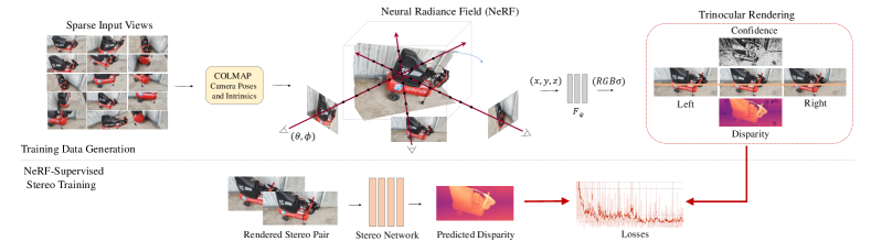
Figure 2: Framework Overview. Top: data generation pipeline that trains NeRFs from user-collected single-camera frames to render stereo images (i.e. triplets), confidence and proxy depth maps. Bottom: NeRF-supervised training of a stereo network on rendered pairs.

2 Related work

Deep Stereo Matching. For decades, stereo matching has been tackled using hand-crafted algorithms [56] usually classified into local and global methods, according to their processing step and their speed/accuracy trade-off. In recent years, deep learning has become the dominant technique in the stereo matching field, achieving results that were previously unthinkable [50]. Early efforts in this field cast individual steps of the pipeline [56] as learnable components [74, 37, 61, 62]. Starting with DispNet [41], end-to-end architectures rapidly replaced any alternative approach [27, 33, 10, 85, 82, 14, 86, 72, 63]. The latest advances in this field take inspiration from RAFT [67] to design recurrent architectures, either by performing lookups on a 3D correlation volume [35] or correlations in a local window [30], or exploiting Transformers [31, 25] to capture long-range dependencies between features of the input stereo pair. Despite their impressive results on public benchmarks, these methods strictly require dense in-domain ground-truth.

Self-Supervised Stereo. This branch of stereo literature aims to train deep models without the use of ground-truth depth data. A common strategy involves using photometric losses [24] across stereo images from single pairs [90, 71, 70] or videos [29, 76, 15]. An alternative line of works replaces it with proxy supervision from either hand-crafted algorithms [68, 69, 49] or distilled from other networks [3]. Although these strategies are practical, they have proven to only be effective at specializing or adapting to single domains, and often lack generalization [3], yet not providing reliable supervision at occlusions. In contrast, we exploit multi-view geometry at its finest through neural rendering to learn for stereo, alike single-image depth estimation frameworks can learn from stereo images [23].

Zero-Shot Generalization. This line of work focuses on training deep models on a set of labeled images and then preserving accuracy when tested across different domains, under the assumption that target domain-specific data is unavailable. Approaches initially explored include: the use of learning domain-invariant features [86], hand-crafted matching volumes [8], or casting disparity estimation as a refinement problem on top of hand-crafted stereo algorithms [2]. The latest trends in the field include using contrastive feature loss and stereo selective whitening loss [87], an ImageNet pre-trained classifier to extract general-purpose image features and graft them into the cost volume [36], or shortcut avoidance [16]. Among others, Mono-for-Stereo (MfS) [79] generates training stereo pairs from large-scale real-world monocular datasets. This at the expense of 1) requiring a pre-trained monocular depth network [53] – which in turns is typically trained on millions of images involving also ground-truth labels – and 2) deal with holes generated by the forward-warping operation used to obtain the right view. In contrast, our approach of generating stereo pairs from single images does not require any model pre-trained on million images [53], ground-truth label or post-processing step, and still achieves better results.

Neural Radiance Fields. NeRFs [44] belong to the family of neural fields [81]. These models implicitly parameterize a 5D lightfield using one or more Multi-Layer Perceptrons (MLPs). In just three years, they have become the dominant approach for generating novel views using neural rendering. Different flavors of NeRFs have been developed to deal with dynamic scenes [39, 52, 32, 80, 19], image relighting [65, 88, 7], camera poses refinement [34, 78], anti-aliasing in multi-resolution images [5, 6], cross-spectral imaging [51], deformable objects [47, 73, 18, 46, 48] or content generation [60, 9, 28]. Most recent NeRF variants focus on faster convergence, e.g. by exploiting multiple MLPs[54], factorization [12] or explicit representations [4, 66, 45].

Recent works partially explored the potential of NeRFs to serve as data factories at high-level – object detection [20], semantic labeling [89] or to learn descriptors [83].

3 Method

Fig. 2 illustrates our NeRF-Supervised (NS) learning framework. We first collect multi-view images from multiple static scenes. Then, we fit a NeRF on each single scene to render stereo triplets and depth. Finally, the rendered data is used to train any existing stereo matching network.

3.1 Background: Neural Radiance Field (NeRF)

A Neural Radiance Field (NeRF) [44] maps a 5D input – 3D coordinates $\mathbf{x}=(x,y,z)$ of a point in the scene and viewing directions $(\theta,\phi)$ of the camera capturing it – into a color-density output $(\mathbf{c},\sigma)$ by means of a network $F_{\psi}$, modelling the radiance of an observed scene as $F_{\psi}(\mathbf{x},\theta,\phi)\rightarrow(\mathbf{c},\sigma)$. Such a 5D function is approximated by the weights of an MLP $F_{\psi}$. To render a 2D image, the following steps are taken: 1) sending camera rays through the scene to sample a set of points, 2) estimate density and color for each sampled point with $F_{\psi}$ and 3) exploit volume rendering [40] to synthesize the 2D image. In practice, the color $C(\mathbf{r})$ rendered from a camera ray $\mathbf{r}(t)=\mathbf{o}+t\mathbf{d}$ can be obtained by solving the following integral:

$$C(\mathbf{r})=\int_{t_{n}}^{t_{f}}T(t)\sigma(\mathbf{r}(t))c(\mathbf{r}(t),\mathbf{d})\textit{dt}$$ (1)

with $T(t)=exp\left(-\int_{t_{n}}^{t}\sigma(\textbf{r}(s))ds\right)$ representing the accumulated transmittance from $t_{n}$ to $t_{f}$ along the ray $r$, and $t_{n},t_{f}$ the near and far plane, respectively. The integral is computed via quadrature by dividing the ray into a pre-defined set of N evenly spaced bins:

$$C(\mathbf{r})=\sum_{i=1}^{N}T_{i}(1-\text{exp}(-\sigma_{i}\delta_{i}))c_{i},\hskip 11.38092ptT_{i}=\text{exp}\Big{(}-{\sum_{j=1}^{i-1}\sigma_{j}\delta_{j}}\Big{)}$$ (2)

with $\delta_{i}$ being the step between adjacent samples $t_{i},t_{i+1}$.

Speed-up with Explicit Representations. The described model is effective, but slow to train due to two reasons: first, the MLP must learn from scratch the mapping for all points in the 5D space and second, for each individual input, the entire set of weights needs to be optimized. Explicit representations – e.g. voxel grids – can store additional features that can be rapidly indexed and interpolated, but this comes at the cost of higher memory requirements. This allows for 1) a shallower MLP, faster to converge and 2) a reduced number of parameters to optimize for each single input – i.e., features on a voxel grid and the few parameters of the shallow MLP. For instance, on this principle, DVGO [66] builds two voxel grids $\mathbf{M}^{\text{(dens)}}$ and $\mathbf{M}^{\text{(feat)}}$, with the former modeling density and the latter storing features that are queried by the MLP $F_{\psi}$ to compute color:

$$\sigma(\mathbf{x}) =\text{interp}(\mathbf{x},\mathbf{M}^{\text{(dens)}})$$ (3)

$$\mathbf{c}(\mathbf{x},\mathbf{d}) =F_{\psi}(\text{interp}(\mathbf{x},\mathbf{M}^{\text{(feat)}}),\mathbf{x},\mathbf{d})$$ (4)

while Instant-NGP [45] builds multi-resolution voxel grids accessed by means of index hashing:

$$h(\mathbf{x})=\Big{(}\bigoplus_{i=0}^{d}x_{i}\pi_{i}\Big{)}\mod{T}$$ (5)

with $\bigoplus$ being bitwise XOR, $x_{i}$ – with $i\in[0,d]$ – single bits of the location index $\mathbf{x}$, $\pi_{i}$ unique, large prime numbers and $T$ the maximum amount of elements in the grid.

\begin{overpic}[width=78.04842pt]{images/0146/left.jpg} \put(0.0,38.0){\color[rgb]{0,1,0}\line(2,0){104.0}} \put(0.0,16.0){\color[rgb]{0,1,0}\line(2,0){104.0}} \put(0.0,4.0){\color[rgb]{0,1,0}\line(2,0){104.0}} \put(0.0,38.0){\color[rgb]{0,1,0}\line(2,0){104.0}} \put(0.0,16.0){\color[rgb]{0,1,0}\line(2,0){104.0}} \put(0.0,4.0){\color[rgb]{0,1,0}\line(2,0){104.0}} \put(0.0,38.0){\color[rgb]{0,1,0}\line(2,0){104.0}} \put(0.0,16.0){\color[rgb]{0,1,0}\line(2,0){104.0}} \put(0.0,4.0){\color[rgb]{0,1,0}\line(2,0){104.0}} \put(0.0,2.0){\hbox{\pagecolor{white}$\displaystyle{\color[rgb]{0,0,0}\text{(a)}}$}} \end{overpic}	\begin{overpic}[width=78.04842pt]{images/0146/center.jpg} \put(0.0,38.0){\color[rgb]{0,1,0}\line(2,0){104.0}} \put(0.0,16.0){\color[rgb]{0,1,0}\line(2,0){104.0}} \put(0.0,4.0){\color[rgb]{0,1,0}\line(2,0){104.0}} \put(0.0,38.0){\color[rgb]{0,1,0}\line(2,0){104.0}} \put(0.0,16.0){\color[rgb]{0,1,0}\line(2,0){104.0}} \put(0.0,4.0){\color[rgb]{0,1,0}\line(2,0){104.0}} \put(0.0,38.0){\color[rgb]{0,1,0}\line(2,0){104.0}} \put(0.0,16.0){\color[rgb]{0,1,0}\line(2,0){104.0}} \put(0.0,4.0){\color[rgb]{0,1,0}\line(2,0){104.0}} \put(0.0,2.0){\hbox{\pagecolor{white}$\displaystyle{\color[rgb]{0,0,0}\text{(b)}}$}} \end{overpic}	\begin{overpic}[width=78.04842pt]{images/0146/right.jpg} \put(0.0,38.0){\color[rgb]{0,1,0}\line(2,0){100.0}} \put(0.0,16.0){\color[rgb]{0,1,0}\line(2,0){100.0}} \put(0.0,4.0){\color[rgb]{0,1,0}\line(2,0){100.0}} \put(0.0,38.0){\color[rgb]{0,1,0}\line(2,0){100.0}} \put(0.0,16.0){\color[rgb]{0,1,0}\line(2,0){100.0}} \put(0.0,4.0){\color[rgb]{0,1,0}\line(2,0){100.0}} \put(0.0,38.0){\color[rgb]{0,1,0}\line(2,0){100.0}} \put(0.0,16.0){\color[rgb]{0,1,0}\line(2,0){100.0}} \put(0.0,4.0){\color[rgb]{0,1,0}\line(2,0){100.0}} \put(0.0,2.0){\hbox{\pagecolor{white}$\displaystyle{\color[rgb]{0,0,0}\text{(c)}}$}} \end{overpic}	\begin{overpic}[width=78.04842pt]{images/0146/nerf_colored.jpg} \put(0.0,2.0){\hbox{\pagecolor{white}$\displaystyle{\color[rgb]{0,0,0}\text{(g)}}$}} \end{overpic}	\begin{overpic}[width=78.04842pt]{images/0146/unc.png} \put(0.0,2.0){\hbox{\pagecolor{white}$\displaystyle{\color[rgb]{0,0,0}\text{(h)}}$}} \end{overpic}
\begin{overpic}[width=78.04842pt]{images/0146/loss_1.jpg} \put(0.0,2.0){\hbox{\pagecolor{white}$\displaystyle{\color[rgb]{0,0,0}\text{(d)}}$}} \end{overpic}	\begin{overpic}[width=78.04842pt]{images/0146/loss_0.jpg} \put(0.0,2.0){\hbox{\pagecolor{white}$\displaystyle{\color[rgb]{0,0,0}\text{(e)}}$}} \end{overpic}	\begin{overpic}[width=78.04842pt]{images/0146/loss.jpg} \put(0.0,2.0){\hbox{\pagecolor{white}$\displaystyle{\color[rgb]{0,0,0}\text{(f)}}$}} \end{overpic}	\begin{overpic}[width=78.04842pt]{images/0146/filtered_nerf_colored.jpg} \put(0.0,2.0){\hbox{\pagecolor{white}$\displaystyle{\color[rgb]{0,0,0}\text{(i)}}$}} \end{overpic}	\begin{overpic}[width=78.04842pt]{images/0146/raft_colored.jpg} \put(0.0,2.0){\hbox{\pagecolor{white}$\displaystyle{\color[rgb]{0,0,0}\text{(j)}}$}}\end{overpic}

Figure 3: Visualization of NS loss components. On the left: (a-c) rendered left-center-right triplet. (d) left-to-center and (e) right-to-center photometric losses, both exposing their own occlusions, (f) per-pixel minimum, compensating for them. On the right: (g) NeRF rendered noisy disparity map, (h) Ambient Occlusion (AO), (i) AO-filtered NeRF disparity, (j) prediction by RAFT-Stereo trained on our dataset.

3.2 NeRF as a Data Factory

With reference to Fig. 2, we now describe, step-by-step, how we use Neural Radiance Fields to generate countless image pairs for training any deep stereo network.

Image Collection and COLMAP Pre-processing. We start by acquiring a sparse set of M images from a single static scene, for which any handheld device with a single camera is suitable, e.g., a mobile phone. We run COLMAP [57] on any single scene to estimate both intrinsics $\mathbf{K}$ and camera poses $\mathbf{E}_{i},i\in[1,\text{M}]$. This is a standard procedure for preparing user-collected data to be NeRFed [44, 5, 6].

NeRF Training. Then, we fit an independent NeRF – in one of its speeded-up flavors [4, 66, 45, 12] – for each scene. This is achieved by rendering, for a given batch $\mathcal{R}$ of rays shot from collected image positions, the corresponding color $\hat{C}(\mathbf{r})$ according to Eq. 2, and optimizing an L2 loss with respect to pixel colors $C(\mathbf{r})$ in the collected frames:

$$\mathcal{L}_{rend}=\sum_{\mathbf{r}\in\mathcal{R}}||\hat{C}(\mathbf{r})-C(\mathbf{r})||_{2}^{2}$$ (6)

Stereo Pairs Rendering. Finally, to create the stereo training set, we generate a virtual set of stereo extrinsic parameters $\mathbf{S}=\mathbb{I}|\mathbf{b}$. The rotation is represented by the $3\times 3$ identity matrix $\mathbb{I}$ and the translation vector $\mathbf{b}=(b,0,0)^{\text{T}}$ has a magnitude $b$ along the $x$ axis in the camera reference system. This defines the baseline of a virtual stereo camera.

Subsequently, we render two novel views, one originating from an arbitrary viewpoint $\mathbf{E}_{k}=\mathbf{R}_{k}|\mathbf{t}_{k}$, and one from its corresponding virtual stereo camera viewpoint $\mathbf{E}_{k}^{\text{R}}=\mathbf{E}_{k}\times\mathbf{S}=\mathbf{R}_{k}|(\mathbf{t}_{k}+\mathbf{b})$, which represent the reference and the target frames of a perfectly rectified stereo pair, with the latter positioned to the right of the former. This process allows for the generation of countless stereo samples for training deep stereo networks. Additionally, for each viewpoint $\mathbf{E}_{k}$, we also render a third image from $\mathbf{E}_{k}^{\text{L}}=\mathbf{E}_{k}\times\mathbf{S}^{-1}=\mathbf{R}_{k}|(\mathbf{t}_{k}-\mathbf{b})$, which is a second target frame placed on the left of the reference one. This creates a stereo triplet in which the three images are perfectly rectified, as shown in Fig. 3 (a-c). The importance of this process, particularly in dealing with occlusions, will be discussed in Sec. 3.3. Finally, we extract the disparity $d_{\mathbf{r}}$ from the rendered depth $z_{\mathbf{r}}$, which is aligned with the center image of the triplet, and use it to assist in the training of any deep stereo network existing in the literature.

$$z(\mathbf{r})=\sum_{i=1}^{N}T_{i}(1-\text{exp}(-\sigma_{i}\delta_{i}))\sigma_{i},\quad\quad d(\mathbf{r})=\frac{b\cdot f}{z(\mathbf{r})}$$ (7)

with $f$ being the focal length estimated by COLMAP [57].

3.3 NeRF-Supervised Training Regime

Data generated so far is then used to train stereo models. Given a rendered image triplet $(I_{l},I_{c},I_{r})$, we estimate a disparity map $\hat{d}_{c}$ by feeding the network with $(I_{c},I_{r})$, which act as the left and right views of a standard stereo pair. Then, we propose an NS loss with two terms.

Triplet Photometric Loss. We exploit image reconstruction to supervise disparity estimation [23]. Specifically, we backward-warp $I_{r}$ according to $\hat{d}_{c}$ and obtain $\hat{I}_{c}^{r}$ – i.e., the reconstructed reference image. Then, we measure the photometric difference between $\hat{I}_{c}^{r}$ and ${I}_{c}$ as:

$$\begin{split}\mathcal{L}_{\rho}(I_{c},\hat{I}_{c}^{r})=\beta\cdot\frac{1-\text{SSIM}(I_{c},\hat{I_{c}^{r}})}{2}+(1-\beta)\cdot|I_{c}-\hat{I}_{c}^{r}|\end{split}$$ (8)

with SSIM being the Structural Similarity Index Measure [77]. Nevertheless, this formulation lacks adequate supervision in occluded regions, such as the left border of the frame or the left of each depth discontinuity, which are not visible in the right image. To overcome this limitation, we employ the third image, $I_{l}$. By computing $\mathcal{L}_{\rho}(I_{c},\hat{I}_{c}^{l})$, the occlusions will be complementary to those from the previous ones. Thus, to compensate for both, we compute the final, triplet photometric loss defined as the per-pixel minimum [24] between the two pairwise terms:

$$\begin{split}\mathcal{L}_{\text{3}\rho}(\hat{I_{l}}^{c},I_{c},\hat{I_{r}}^{c})=\min\Biggl{(}\mathcal{L}_{\rho}(\hat{I_{l}}^{c},I_{c}),\mathcal{L}_{\rho}(I_{c},\hat{I_{r}}^{c})\Biggr{)}\end{split}$$ (9)

Fig. 3 (left) shows the effect of occlusions when computing $\mathcal{L}_{\rho}$ between center-left (d) and center-right (e) pairs with bright colors, whereas they are neglected by $\mathcal{L}_{3\rho}$ (f). Finally, untextured regions are discarded by a mask $\mu$ [24]:

$$\mu=[\min\mathcal{L}_{\text{3}\rho}(\hat{I_{l}}^{c},I_{c},\hat{I_{r}}^{c})<\min\mathcal{L}_{\text{3}\rho}(I_{l},I_{c},I_{r})]$$ (10)

Rendered Disparity Loss. We further assist the photometric loss by exploiting rendered disparities as:

$$\mathcal{L}_{disp}=|d_{c}-\hat{d}_{c}|$$ (11)

However, depth maps rendered by NeRF often exhibit artifacts and large errors [17], as shown in Fig. 3 (g). To address this issue, we employ a filtering mechanism to preserve only the most reliable pixels. We use Ambient Occlusion (AO) [45] to measure the confidence of $d_{c}$:

$$\text{AO}=\sum_{i=1}^{N}T_{i}\alpha_{i},\quad\quad\alpha_{i}=1-\text{exp}(-\sigma_{i}\delta_{i})$$ (12)

and will use it to filter the disparity loss accordingly. More details are discussed in the supplementary material.

NeRF-Supervised Loss. The two terms are summed as:

$$\begin{split}\mathcal{L}_{NS}&=\gamma_{disp}\cdot\eta_{disp}\cdot\mathcal{L}_{disp}\\ &+\mu\cdot\gamma_{\text{3}\rho}\cdot(1-\eta_{disp})\cdot\mathcal{L}_{\text{3}\rho}\end{split}$$ (13)

with $\gamma_{disp},\gamma_{3\rho}$ being weights balancing the impact of photometric and disparity losses, and $\eta_{disp}$ being defined as:

$$\eta_{disp}=\begin{cases}0&\text{if }\text{AO}<th\\ \text{AO}&\text{otherwise }\\ \end{cases}$$ (14)

according to a threshold $th$ over AO, normalized in $[0,1]$.

	2-views		3-views
								KITTI-12	Midd-A			Midd-21
	$\mathcal{L}_{\rho}$	SGM	$\mathcal{L}_{\text{3}\rho}$	SGM	$\mathcal{L}_{disp}$	$>th$	$\eta_{disp}$	($>3$px)	F ($>2$px)	H ($>2$px)	Q ($>2$px)	($>2$px)
(A)	✓							11.00	56.05	32.33	25.60	44.88
(B)		✓						6.39	22.68	17.23	18.14	23.71
(B’)		[3]✓						5.46	19.50	15.26	17.36	21.29
(C)			✓					5.11	28.33	13.57	12.09	24.38
(D)				✓				5.57	19.10	13.22	14.91	20.08
(E)					✓			5.79	21.71	9.85	8.73	22.69
(F)					✓	✓		4.49	15.50	9.25	9.13	16.99
(G)	✓				✓	✓		4.31	16.11	9.57	9.96	16.83
(H)			✓		✓	✓		4.21	15.31	8.86	8.41	16.26
(I)			✓		✓	✓	✓	4.31	14.92	8.75	8.28	14.87
(I’)			✓		✓	✓	✓	4.02	13.12	6.91	7.18	12.87

Table 1: Ablation Study – Loss Components. Impact of each component in our NS loss. [3]$\checkmark$ means using SGM plus [3].

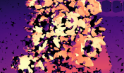
\begin{overpic}[height=37.2627pt]{images/0074/center.jpg} \put(0.0,2.0){\hbox{\pagecolor{white}$\displaystyle{\color[rgb]{0,0,0}\text{(a)}}$}} \end{overpic}	\begin{overpic}[height=37.2627pt]{images/0074/nerf.jpg} \put(0.0,2.0){\hbox{\pagecolor{white}$\displaystyle{\color[rgb]{0,0,0}\text{(b)}}$}} \end{overpic}	\begin{overpic}[height=37.2627pt]{images/0074/raft_bino.png} \put(0.0,2.0){\hbox{\pagecolor{white}$\displaystyle{\color[rgb]{0,0,0}\text{(c)}}$}} \put(23.0,28.0){\color[rgb]{0,1,0}\line(2,0){10.0}} \put(23.0,28.0){\color[rgb]{0,1,0}\line(0,-2){28.0}} \put(33.0,28.0){\color[rgb]{0,1,0}\line(0,-2){28.0}} \put(23.0,0.0){\color[rgb]{0,1,0}\line(2,0){10.0}} \put(23.0,28.0){\color[rgb]{0,1,0}\line(2,0){10.0}} \put(23.0,28.0){\color[rgb]{0,1,0}\line(0,-2){28.0}} \put(33.0,28.0){\color[rgb]{0,1,0}\line(0,-2){28.0}} \put(23.0,0.0){\color[rgb]{0,1,0}\line(2,0){10.0}} \put(23.0,28.0){\color[rgb]{0,1,0}\line(2,0){10.0}} \put(23.0,28.0){\color[rgb]{0,1,0}\line(0,-2){28.0}} \put(33.0,28.0){\color[rgb]{0,1,0}\line(0,-2){28.0}} \put(23.0,0.0){\color[rgb]{0,1,0}\line(2,0){10.0}} \put(23.0,28.0){\color[rgb]{0,1,0}\line(2,0){10.0}} \put(23.0,28.0){\color[rgb]{0,1,0}\line(0,-2){28.0}} \put(33.0,28.0){\color[rgb]{0,1,0}\line(0,-2){28.0}} \put(23.0,0.0){\color[rgb]{0,1,0}\line(2,0){10.0}} \end{overpic}	\begin{overpic}[height=37.2627pt]{images/0074/raft_trino.png} \put(0.0,2.0){\hbox{\pagecolor{white}$\displaystyle{\color[rgb]{0,0,0}\text{(d)}}$}} \put(23.0,28.0){\color[rgb]{0,1,0}\line(2,0){10.0}} \put(23.0,28.0){\color[rgb]{0,1,0}\line(0,-2){28.0}} \put(33.0,28.0){\color[rgb]{0,1,0}\line(0,-2){28.0}} \put(23.0,0.0){\color[rgb]{0,1,0}\line(2,0){10.0}} \put(23.0,28.0){\color[rgb]{0,1,0}\line(2,0){10.0}} \put(23.0,28.0){\color[rgb]{0,1,0}\line(0,-2){28.0}} \put(33.0,28.0){\color[rgb]{0,1,0}\line(0,-2){28.0}} \put(23.0,0.0){\color[rgb]{0,1,0}\line(2,0){10.0}} \put(23.0,28.0){\color[rgb]{0,1,0}\line(2,0){10.0}} \put(23.0,28.0){\color[rgb]{0,1,0}\line(0,-2){28.0}} \put(33.0,28.0){\color[rgb]{0,1,0}\line(0,-2){28.0}} \put(23.0,0.0){\color[rgb]{0,1,0}\line(2,0){10.0}} \put(23.0,28.0){\color[rgb]{0,1,0}\line(2,0){10.0}} \put(23.0,28.0){\color[rgb]{0,1,0}\line(0,-2){28.0}} \put(33.0,28.0){\color[rgb]{0,1,0}\line(0,-2){28.0}} \put(23.0,0.0){\color[rgb]{0,1,0}\line(2,0){10.0}} \end{overpic}	\begin{overpic}[height=37.2627pt]{images/0074/raft_ours.png} \put(0.0,2.0){\hbox{\pagecolor{white}$\displaystyle{\color[rgb]{0,0,0}\text{(e)}}$}} \put(23.0,28.0){\color[rgb]{0,1,0}\line(2,0){10.0}} \put(23.0,28.0){\color[rgb]{0,1,0}\line(0,-2){28.0}} \put(33.0,28.0){\color[rgb]{0,1,0}\line(0,-2){28.0}} \put(23.0,0.0){\color[rgb]{0,1,0}\line(2,0){10.0}} \put(23.0,28.0){\color[rgb]{0,1,0}\line(2,0){10.0}} \put(23.0,28.0){\color[rgb]{0,1,0}\line(0,-2){28.0}} \put(33.0,28.0){\color[rgb]{0,1,0}\line(0,-2){28.0}} \put(23.0,0.0){\color[rgb]{0,1,0}\line(2,0){10.0}} \put(23.0,28.0){\color[rgb]{0,1,0}\line(2,0){10.0}} \put(23.0,28.0){\color[rgb]{0,1,0}\line(0,-2){28.0}} \put(33.0,28.0){\color[rgb]{0,1,0}\line(0,-2){28.0}} \put(23.0,0.0){\color[rgb]{0,1,0}\line(2,0){10.0}} \put(23.0,28.0){\color[rgb]{0,1,0}\line(2,0){10.0}} \put(23.0,28.0){\color[rgb]{0,1,0}\line(0,-2){28.0}} \put(33.0,28.0){\color[rgb]{0,1,0}\line(0,-2){28.0}} \put(23.0,0.0){\color[rgb]{0,1,0}\line(2,0){10.0}} \end{overpic}

Figure 4: Effect of Training Losses. On the left: (a) center image and (b) corresponding disparity rendered by NeRF. On the right: disparity maps (and zoom-in) by RAFT-Stereo trained with (c) center-right or (d) triplet photometric loss, and (e) our full NeRF-Supervised loss.

4 Experimental Results

We introduce our experiments, first describing implementation details, datasets and, then, discussing our results.

4.1 Implementation Details

All experiments are conducted on a single 3090 NVIDIA GPU (more details in the supplementary material).

Training Data Generation. We collect a total of 270 high-resolution scenes in both indoor and outdoor environments using standard camera-equipped smartphones. For each scene, we focus on a/some specific object(s) and acquire 100 images from different viewpoints, ensuring that the scenery is completely static. The acquisition protocol involves a set of either front-facing or $360\mathrm{°}$ views. We use Instant-NGP [45] as the NeRF engine in our pipeline and train it for 50K steps. Running COLMAP and training Instant-NGP takes $\sim 25$ minutes per scene, with the collected images having a resolution of $\sim 8$Mpx. Afterwards, we generate data with three virtual baselines of $b=0.5,0.3$ and $0.1$ units at different resolutions. We render a disparity map and a triplet from any image used to train Instant-NGP, aligning the center view to the original viewpoint. This results in a total of 65,148 triplets for training. Although more triplets could have been rendered ( i.e., using additional random viewpoints and baselines), these are sufficient to achieve outstanding results.

Deep Stereo Training. We adopt RAFT-Stereo [35] as the main architecture over which we build our evaluation due to its accuracy and fast convergence. Yet, we also consider PSMNet [10] and CFNet [63] to evaluate the effectiveness of our proposal on widely used stereo backbones. We train all models on our dataset with batch size of 2 and a crop size of $384\times 768$. We run 200k training steps for RAFT-Stereo and 250k for PSMNet and CFNet. For ablation experiments, we run 100k iterations following [35]. All the networks are trained from scratch without any pre-training on synthetic datasets. The augmentation procedure described in [35] is used for training. For PSMNet and CFNet, we set $d_{max}$ to 256 and disabled ImageNet normalization. We use learning rate schedules and optimizers as in [35, 10, 63]. In our experiments, we fix $\beta=0.85$, $th=0.5$, $\gamma_{\text{3}\rho}=0.1$ and $\gamma_{disp}=1$.

4.2 Evaluation Datasets & Protocol

We use the KITTI [22], Middlebury [55] and ETH3D [59] datasets with publicly available ground-truth for evaluation. Specifically, we define validation and testing splits.

Validation: 194 stereo images from KITTI 2012, 13 Additional images from the training set of Middlebury v3 (Midd-A) at Full, Half and Quarter resolutions (F, H, Q), and the Middlebury 2021 (Midd-21) dataset. On this split, we run ablation studies and direct comparisons with MfS [79].

Testing: 200 stereo images from KITTI 2015, 15 stereo pairs from Middlebury v3 training set (Midd-T) and 27 pairs from ETH3D. On them, we compare with existing methods that perform zero-shot generalization [86, 16, 87, 36].

Evaluation Metrics. During evaluation, we compute the percentage of pixels having a disparity error greater than a given threshold $\tau$ with respect to the ground-truth. Specifically, we fix $\tau=3$ for KITTI, $\tau=2$ for Middlebury, $\tau=1$ for ETH3D, following the common protocol in the stereo matching field. Unless stated otherwise, we evaluate the computed disparity maps considering both occluded as well as non-occluded regions with valid ground-truth disparity.

Baseline			KITTI-12	Midd-A			Midd- 21
0.5	0.3	0.1	($>3$px)	F ($>2$px)	H ($>2$px)	Q ($>2$px)	($>2$px)
✓	-	-	3.97	18.71	10.55	12.09	16.70
✓	✓	-	3.92	16.77	9.66	10.62	16.96
✓	✓	✓	4.31	14.92	8.75	8.28	14.87

Table 2: Ablation Study – Impact of Baselines. We render triplets with large, medium or small baselines – 0.5, 0.3, 0.1 units.

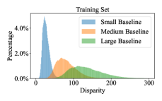
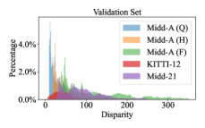
Figure 5: Disparity Distributions. On the left: our rendered dataset. On the right: datasets from the validation split.

4.3 Ablation Study

We ablate our NS loss and its impact on the training process, as well as other properties of our rendered dataset.

Loss Analysis. Tab. 1 shows the results of various instances of RAFT-Stereo trained using different variations of our NS loss. We start by motivating the use of $\mathcal{L}_{\rho}$: by training the model using a conventional self-supervised loss on stereo pairs (A) leads to poor performance. This is mainly due to occlusions, for which no supervision can be provided. By using proxy-labels obtained through SGM [26] and filtering them with a näive left-right consistency check to remove outliers at occlusions (B), the error rates are halved. The same labels processed by [3] further improve the results significantly (B’). However, by exploiting the triplets peculiar to our dataset, $\mathcal{L}_{3\rho}$ alone (C) outperforms both (A) and (B), thanks to the stronger self-supervision recovered at occlusions. Interestingly, labels extracted by [3] (B’) still produce better performance on the high-resolution datasets Midd-A (F) and Midd-21, despite being outperformed by SGM labels over triplets (D).

Resolution		KITTI-12	Midd-A			Midd- 21
$\sim 2$Mpx	$\sim 0.5$Mpx	($>3$px)	F ($>2$px)	H ($>2$px)	Q ($>2$px)	($>2$px)
✓	-	5.34	14.77	11.56	12.32	15.53
-	✓	4.31	14.92	8.75	8.28	14.87
✓	✓	4.42	13.92	9.12	9.66	15.88

Table 3: Ablation Study – Impact of Rendering Resolution. We render images at both half and quarter of the native resolution.

# Scenes			KITTI-12	Midd-A			Midd- 21
65	135	270	($>3$px)	F ($>2$px)	H ($>2$px)	Q ($>2$px)	($>2$px)
✓	-	-	3.98	18.23	11.07	11.30	17.44
-	✓	-	3.87	15.82	9.69	10.36	16.51
-	-	✓	4.31	14.92	8.75	8.28	14.87

Table 4: Ablation Study – Number of Collected Scenes. We render images from different amounts of collected scenes.

(A) (B) (C) (D) (E) (F) (G) (H) (I)

Configuration KITTI-12 Midd-A Midd-21 Model Stereo Network Dataset # Images Pre-Train. ($>3$px) F ($>2$px) H ($>2$px) Q ($>2$px) ($>2$px) MfS[79] + MidAs PSMNet MfS 535K $\sim$2M 4.70 25.61 17.98 14.78 27.55 MfS[79] + MidAs PSMNet Ours 65K $\sim$2M 5.02 28.72 20.66 16.92 26.40 NS (Ours) PSMNet Ours 65K 0 4.07 19.84 13.66 9.15 19.08 MfS[79] + MidAs CFNet MfS 535K $\sim$2M 4.47 22.00 16.69 14.32 23.44 MfS[79] + MidAs CFNet Ours 65K $\sim$2M 4.90 24.20 19.11 16.20 23.76 NS (Ours) CFNet Ours 65K 0 4.64 17.55 12.31 11.13 19.73 MfS[79] + MidAs RAFT-Stereo MfS 535K $\sim$2M 4.45 19.79 12.67 9.63 22.26 MfS[79] + MidAs RAFT-Stereo Ours 65K $\sim$2M 4.67 24.61 17.25 14.05 24.18 NS (Ours) RAFT-Stereo Ours 65K 0 4.02 13.12 6.91 7.18 12.87

Table 5: Direct Comparison with MfS [79]. We report results achieved by networks trained using MfS pipeline – both with their proposed dataset and ours – and trained with our NeRF-supervised approach (NS).

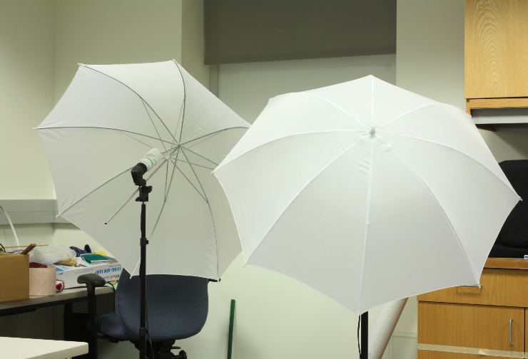
	\begin{overpic}[width=79.49881pt]{images/qualitative-main/umbrella_mfs.jpg} \end{overpic}
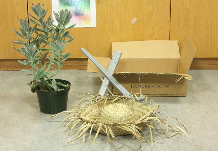
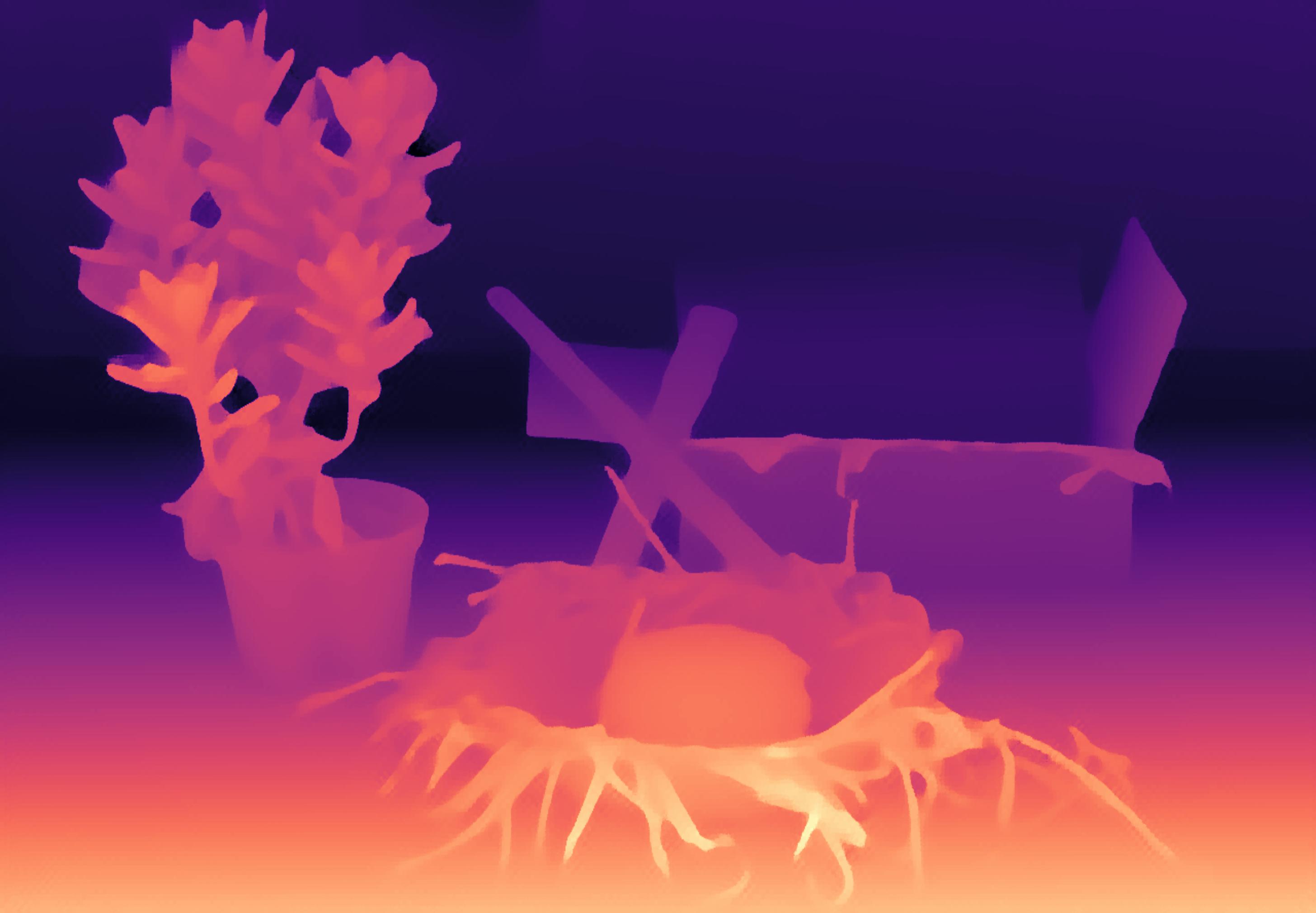
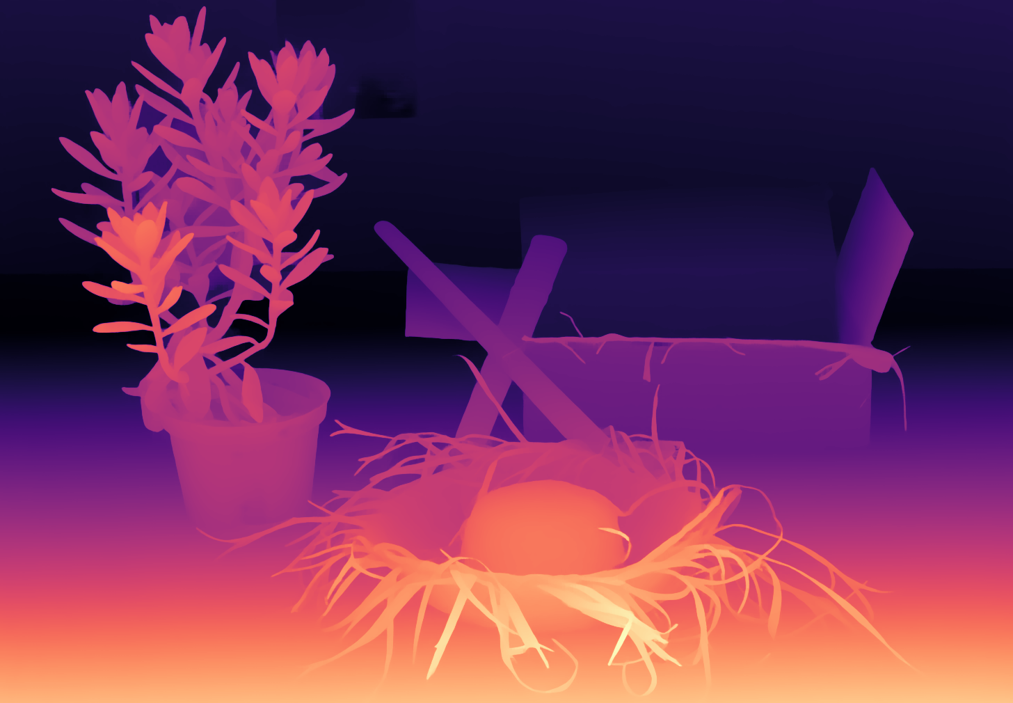
($>2$px)	MfS: 20.47%	Ours: 6.57%		MfS: 8.97%	Ours: 4.74%
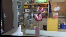
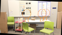
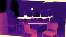
($>2$px)	MfS: 14.41%	Ours: 6.63%		MfS: 24.45%	Ours: 3.57%

Figure 6: Qualitative Comparison on Midd-A H (top) and Midd-21 (bottom) Datasets. From left to right: left images and disparity maps by RAFT-Stereo models, respectively trained with MfS or NS. Under each disparity map, the percentage of pixels with error $>2$.

Considering the superiority of proxy labels over photometric losses alone, we then exploit the disparity maps rendered by NeRF to supervise the stereo model (E), resulting in mixed results – i.e. better on low-resolution Middlebury but worse on Midd-A (F), Midd-21 and KITTI. Indeed, such a supervision alone results sub-optimal due to the several artefacts shown in Fig. 3 (g) and recurring in most scenes, making it less effective than $\mathcal{L}_{3\rho}$ on KITTI, Midd-A (F) and Midd-21. By neglecting the contribution of labels having AO$<th$, results dramatically improve for KITTI and high-resolution datasets, with a minor drop on Midd-A (Q). Instead, a major improvement is obtained over all datasets by combining $\mathcal{L}_{disp}$ with $\mathcal{L}_{3\rho}$ (H). The triplet is crucial for this: combining $\mathcal{L}_{disp}$ with $\mathcal{L}_{\rho}$ is less effective (G).

Finally, our full $\mathcal{L}_{NS}$ loss (I), balancing the two terms according to AO, results the most effective on the validation split. Furthermore, row (I’) shows the impact of a longer training schedule (200K steps vs 100K). Fig. 4 qualitatively shows how the estimated disparities by RAFT-Stereo improve dramatically when switching from conventional image loss (c) to $\mathcal{L}_{3\rho}$ (d), although finer details are still missing. $\mathcal{L}_{NS}$ recovers them with unprecedented fidelity (e).

(A) (B) (C) (D)

KITTI-15 Midd-T ETH3D Method ($>3$px) F ($>2$px) H ($>2$px) Q ($>2$px) ($>1$px) All Noc All Noc All Noc All Noc All Noc Training Set SceneFlow with GT GANet [85] 10.46 10.15 45.36 40.80 26.75 21.8 15.52 11.49 8.68 7.75 DSMNet [86] 5.50 5.19 29.95 24.79 16.88 12.03 13.75 9.44 12.52 11.62 CFNet [63] 6.01 5.94 29.12 24.15 20.11 15.84 13.77 10.32 5.77 5.32 MS-GCNet [8] * 6.21 - - - - 18.52 - - - 8.84 3-12 RAFT-Stereo [35] * 5.74 - 18.33 - 12.59 - 9.36 - 3.28 - RAFT-Stereo [35] ‡ 5.45 5.21 18.20 14.19 11.19 8.09 9.31 6.56 2.59 2.24 3-12 SGM + NDR [2] 5.41 5.12 27.27 21.09 17.70 13.51 11.75 7.93 5.20 4.78 STTR [31] 8.31 6.73 38.10 30.74 26.39 18.17 15.91 8.51 20.49 19.06 CEST [25] 7.61 6.13 27.44 19.53 19.89 11.82 14.71 7.56 10.99 9.78 FC-GANet [87] * 5.3x - - - - 10.2x - 7.8x 5.8x - ITSA-GWCNet [16] 5.60 5.39 29.46 25.18 19.38 15.95 14.36 10.76 7.43 7.12 ITSA-CFNet [16] 4.96 4.76 26.38 21.41 18.01 14.00 13.32 9.73 5.40 5.14 CREStereo [30] ‡ 5.79 5.40 34.78 30.52 17.57 13.87 12.88 8.85 8.98 8.14 PSMNet [10] ‡ 7.86 7.40 33.69 28.35 21.69 16.92 17.24 12.37 23.19 22.12 MS-PSMNet [8] * 7.76 - - - - 19.81 - - - 16.84 Graft-PSMNet[36] 5.34 5.02 25.46 19.28 17.81 13.46 14.18 9.21 11.42 10.69 FC-PSMNet [87] * 5.8x - - - - 15.1x - 9.3x 9.5x - ITSA-PSMNet [16] 6.00 5.73 32.09 27.46 20.83 17.14 14.68 11.05 10.34 9.77 Training Set Real-world data without GT Reversing[3]-PSMNet $[4.09]$ $[3.88]$ 38.23 30.00 26.45 20.91 20.55 15.08 9.00 8.23 MfS[79]-PSMNet 5.18 4.91 26.42 21.38 17.56 13.45 12.07 9.09 8.17 7.44 NS-PSMNet (Ours) 5.05 4.80 20.60 15.83 12.91 9.07 11.03 7.15 11.69 11.00 NS-RAFT-Stereo (Ours) 5.41 5.23 16.45 12.08 9.67 6.42 8.05 4.82 2.94 2.23

Table 6: Zero-Shot Generalization Benchmark. We test all models using authors’ weights. Exceptions: $*$ numbers from the original paper; ‡ retrained model. Best results per macro-block in bold. We also highlight first, second and third absolute bests. For RAFT-Stereo (in dashed lines) only the best between $*$ and ‡ is kept for rankings. $[\kern 1.79997pt]$ means trained on the same domain, thus ignored for rankings.

Impact of Virtual Baselines. We evaluate the impact of the virtual baseline used to render triplets on the disparity distribution. Tab. 2 shows the results of our study on the training effectiveness. Specifically, we render our dataset using a single, large baseline of 0.5 units (21,716 triplets), as well as adding more images obtained with medium and small baselines of 0.3 and 0.1 units. We can observe that using only the large one yields the best results on KITTI, while rendering additional images with the medium baseline results in improvements on Midd-A only. Utilizing all three baselines leads to the best results on Midd-A and Midd-21, with a moderate drop on KITTI. We ascribe this to the disparity distributions generated by using the three baselines, that covers the full range defined by the combined validation sets, as shown in Fig. 5.

Impact of Image Resolution. We evaluate the impact of image resolution on the training process. Purposely, we render images at approximately 2 and 0.5Mpx out of the original 8Mpx images – this because, in terms of computational burden, existing stereo networks can rarely deal with them, despite our pipeline would perfectly allow for this. As shown in Tab. 3, the best results are usually obtained by rendering 0.5Mpx images, except when testing at full resolution on Midd-A, for which rendering both higher and lower resolution images provides benefits.

Impact of Scenes. Finally, we show the impact of a larger number of collected scenes on the training process. Tab. 4 highlights how the accuracy on the most challenging datasets – i.e., Middlebury – increases with it, unsurprisingly. This represents a key strength of our work, enabling anyone to generate their own extensive and scalable training data collections for stereo, resulting in better and better results, thanks to its ease of implementation.

4.4 Comparison with MfS

To further evaluate the quality of our rendered data, we compare our approach with MfS [79] – the most recent method for generating stereo pairs from single images – by training three different stereo networks. Tab. 5 collects the outcome of this experiment using PSMNet [10], i.e. the baseline model used in [79], as well as with CFNet [63] and RAFT-Stereo [35]. Each model is trained on the dataset proposed in [79] (A,D,G), as well as on stereo pairs generated with their technique on our data (B,E,H) or by means of our NS paradigm (C,F,I). We point out that in the first two cases, 2 million labeled images were used to train MidAS [53], which is the key component of their pipeline. In contrast, our approach does not require any additional data.

First, we note that using the MfS generation method on our data consistently leads to inferior results compared to using theirs – i.e. (B) vs (A), (E) vs (D), (H) vs (G). This is unsurprising, considering that our images were collected from only 270 scenes, while the original dataset used by MfS includes half a million images from COCO, ADE20K, DIODE, Mapillary, and DiW, which provide a much wider range of scenes and contexts. This excludes the fact that the superior results achieved by NS are a consequence of the quality of collected images solely. Eventually, any network trained with the NS supervision granted by our data, always outperforms its two counterparts by a large margin – except with CFNet on KITTI, where we register a 0.17% drop. This proves that our paradigm is effective with different stereo architectures and consistently outperforms MfS without the need for a large training dataset.

Finally, Fig. 6 shows a comparison between RAFT-Stereo trained with MfS on the dataset adopted in [79], and its NS counterpart. The results showcase the much more detailed predictions of the latter, especially in thin structures, which is of unprecedented quality for methods not trained on ground-truth. More are reported in the supplement.

4.5 Zero-Shot Generalization Benchmark

We conclude by evaluating stereo networks trained in an NS manner for zero-shot generalization. Table 6 collects the comparison with several state-of-the-art methods on the benchmark common to the latest works [16, 87, 36].

It is worth mentioning that different papers have often evaluated with different protocols on the Middlebury dataset: some compute the metrics only for Noc regions [36, 16], some limit the set of valid pixels to those having ground-truth disparity lower than 192[36, 16], and others compute a weighted average over the dataset, setting challenging images to 0.5 as indicated on the Middlebury website [3, 16]. The protocol itself is often not reported in the papers, leading to the accumulation of several inconsistencies throughout the literature and, possibly, drawing biased conclusions. To address this, we re-evaluated any method with available code and weights, both over All / Noc pixels and considering the entire disparity range, to establish a common protocol from now on. For a few methods whose weights are no longer available, we either took numbers from the original paper ($*$), although they may not be entirely comparable with the others, or retrained them (‡).

We defined four main groups of methods: (A) existing stereo models, excluding (B) PSMNet variants, both of which were trained on synthetic data with ground-truth; (C) PSMNet models trained without ground-truth; and (D) our best model. (B) and (C) allow for comparison of several methods pursuing generalization while using a common backbone. We can see that our NS-PSMNet outperforms all PSMNet variants, except on ETH3D (it is worth noting that Reversing-PSMNet [3] was trained on raw KITTI [23], which gives it a significant advantage). Among the methods in group (A), only RAFT-Stereo outperforms NS-PSMNet on Middlebury, but performs worse on KITTI, where ITSA-CFNet is the best method among all. This suggests that RAFT-Stereo already has strong generalization capability. Combining RAFT-Stereo with NS (group D) consistently produces the best results across the entire Middlebury dataset, and results that are equivalent to RAFT-Stereo trained on synthetic ground-truth on ETH3D, all without requiring any ground-truth data. This results in a small drop in accuracy on KITTI, that is negligible in exchange for the improvement on Middlebury (often 30-40%).

5 Conclusion

We have presented a pioneering pipeline that leverages NeRF to train deep stereo networks without the requirement of ground-truth depth or stereo cameras. By capturing images with a single low-cost handheld camera, we generate thousands of stereo pairs for training through our NS paradigm. This approach results in state-of-the-art zero-shot generalization, surpassing both self-supervised and supervised methods. Our work represents a significant advancement towards data democratization, putting the key to the success into the users’ hands.

Limitations. Samples collected so far are limited to small-scale, static scenes. Moreover, our NS – and any – stereo networks still fail in some challenging conditions, e.g. transparent surfaces [84] or nighttime images [21, 11]. A larger-scale collection campaign, coupled with other NeRFs variants [43, 64], may deal with them in the future.

Future Research. Our NS pipeline can possibly be extended to generate labels for other dense, low-level tasks such as optical flow (similarly to [1]) or multi-view stereo.

References

- [1] Filippo Aleotti, Matteo Poggi, and Stefano Mattoccia. Learning optical flow from still images. In IEEE/CVF Conference on Computer Vision and Pattern Recognition (CVPR), 2021.
- [2] Filippo Aleotti, Fabio Tosi, Pierluigi Zama Ramirez, Matteo Poggi, Samuele Salti, Luigi Di Stefano, and Stefano Mattoccia. Neural disparity refinement for arbitrary resolution stereo. In International Conference on 3D Vision, 2021. 3DV.
- [3] Filippo Aleotti, Fabio Tosi, Li Zhang, Matteo Poggi, and Stefano Mattoccia. Reversing the cycle: self-supervised deep stereo through enhanced monocular distillation. In 16th European Conference on Computer Vision (ECCV). Springer, 2020.
- [4] Alex Yu and Sara Fridovich-Keil, Matthew Tancik, Qinhong Chen, Benjamin Recht, and Angjoo Kanazawa. Plenoxels: Radiance fields without neural networks, 2021.
- [5] Jonathan T. Barron, Ben Mildenhall, Matthew Tancik, Peter Hedman, Ricardo Martin-Brualla, and Pratul P. Srinivasan. Mip-nerf: A multiscale representation for anti-aliasing neural radiance fields. In Proceedings of the IEEE/CVF International Conference on Computer Vision (ICCV), pages 5855–5864, October 2021.
- [6] Jonathan T Barron, Ben Mildenhall, Dor Verbin, Pratul P Srinivasan, and Peter Hedman. Mip-nerf 360: Unbounded anti-aliased neural radiance fields. In Proceedings of the IEEE/CVF Conference on Computer Vision and Pattern Recognition, pages 5470–5479, 2022.
- [7] Mark Boss, Raphael Braun, Varun Jampani, Jonathan T. Barron, Ce Liu, and Hendrik P. A. Lensch. Nerd: Neural reflectance decomposition from image collections. In ICCV, 2021.
- [8] Changjiang Cai, Matteo Poggi, Stefano Mattoccia, and Philippos Mordohai. Matching-space stereo networks for cross-domain generalization. In 2020 International Conference on 3D Vision (3DV), pages 364–373, 2020.
- [9] Eric R. Chan, Marco Monteiro, Petr Kellnhofer, Jiajun Wu, and Gordon Wetzstein. Pi-gan: Periodic implicit generative adversarial networks for 3d-aware image synthesis. In CVPR, 2021.
- [10] Jia-Ren Chang and Yong-Sheng Chen. Pyramid stereo matching network. In IEEE/CVF Conference on Computer Vision and Pattern Recognition (CVPR), pages 5410–5418, 2018.
- [11] Ming-Fang Chang, John W Lambert, Patsorn Sangkloy, Jagjeet Singh, Slawomir Bak, Andrew Hartnett, De Wang, Peter Carr, Simon Lucey, Deva Ramanan, and James Hays. Argoverse: 3d tracking and forecasting with rich maps. In Conference on Computer Vision and Pattern Recognition (CVPR), 2019.
- [12] Anpei Chen, Zexiang Xu, Andreas Geiger, Jingyi Yu, and Hao Su. Tensorf: Tensorial radiance fields. In European Conference on Computer Vision (ECCV), 2022.
- [13] Zhi Chen, Xiaoqing Ye, Wei Yang, Zhenbo Xu, Xiao Tan, Zhikang Zou, Errui Ding, Xinming Zhang, and Liusheng Huang. Revealing the reciprocal relations between self-supervised stereo and monocular depth estimation. In Proceedings of the IEEE/CVF International Conference on Computer Vision, pages 15529–15538, 2021.
- [14] Xuelian Cheng, Yiran Zhong, Mehrtash Harandi, Yuchao Dai, Xiaojun Chang, Hongdong Li, Tom Drummond, and Zongyuan Ge. Hierarchical neural architecture search for deep stereo matching. Advances in Neural Information Processing Systems, 33, 2020.
- [15] Cheng Chi, Qingjie Wang, Tianyu Hao, Peng Guo, and Xin Yang. Feature-level collaboration: Joint unsupervised learning of optical flow, stereo depth and camera motion. In Proceedings of the IEEE/CVF Conference on Computer Vision and Pattern Recognition, pages 2463–2473, 2021.
- [16] WeiQin Chuah, Ruwan Tennakoon, Reza Hoseinnezhad, Alireza Bab-Hadiashar, and David Suter. Itsa: An information-theoretic approach to automatic shortcut avoidance and domain generalization in stereo matching networks. In Proceedings of the IEEE/CVF Conference on Computer Vision and Pattern Recognition, pages 13022–13032, 2022.
- [17] Kangle Deng, Andrew Liu, Jun-Yan Zhu, and Deva Ramanan. Depth-supervised nerf: Fewer views and faster training for free. In Proceedings of the IEEE/CVF Conference on Computer Vision and Pattern Recognition, pages 12882–12891, 2022.
- [18] Guy Gafni, Justus Thies, Michael Zollhöfer, and Matthias Nießner. Dynamic neural radiance fields for monocular 4d facial avatar reconstruction. In CVPR, 2021.
- [19] Chen Gao, Ayush Saraf, Johannes Kopf, and Jia-Bin Huang. Dynamic view synthesis from dynamic monocular video. In ICCV, 2021.
- [20] Yunhao Ge, Harkirat Behl, Jiashu Xu, Suriya Gunasekar, Neel Joshi, Yale Song, Xin Wang, Laurent Itti, and Vibhav Vineet. Neural-sim: Learning to generate training data with nerf. In European Conference on Computer Vision, pages 477–493. Springer, 2022.
- [21] Mathias Gehrig, Willem Aarents, Daniel Gehrig, and Davide Scaramuzza. Dsec: A stereo event camera dataset for driving scenarios. IEEE Robotics and Automation Letters, 2021.
- [22] Andreas Geiger, Philip Lenz, and Raquel Urtasun. Are we ready for autonomous driving? the kitti vision benchmark suite. In Conference on Computer Vision and Pattern Recognition (CVPR), 2012.
- [23] Clément Godard, Oisin Mac Aodha, and Gabriel J. Brostow. Unsupervised monocular depth estimation with left-right consistency. In CVPR, 2017.
- [24] Clement Godard, Oisin Mac Aodha, Michael Firman, and Gabriel J. Brostow. Digging into self-supervised monocular depth estimation. In IEEE International Conference on Computer Vision (ICCV), 2019.
- [25] Weiyu Guo, Zhaoshuo Li, Yongkui Yang, Zheng Wang, Russell H Taylor, Mathias Unberath, Alan Yuille, and Yingwei Li. Context-enhanced stereo transformer. In Proceedings of the European Conference on Computer Vision (ECCV), 2022.
- [26] Heiko Hirschmuller. Stereo processing by semiglobal matching and mutual information. IEEE Transactions on pattern analysis and machine intelligence, 30(2):328–341, 2007.
- [27] Alex Kendall, Hayk Martirosyan, Saumitro Dasgupta, Peter Henry, Ryan Kennedy, Abraham Bachrach, and Adam Bry. End-to-end learning of geometry and context for deep stereo regression. In The IEEE International Conference on Computer Vision (ICCV), Oct 2017.
- [28] Adam R. Kosiorek, Heiko Strathmann, Daniel Zoran, Pol Moreno, Rosalia Schneider, Sona Mokrá, and Danilo Jimenez Rezende. Nerf-vae: A geometry aware 3d scene generative model. In ICML, 2021.
- [29] Hsueh-Ying Lai, Yi-Hsuan Tsai, and Wei-Chen Chiu. Bridging stereo matching and optical flow via spatiotemporal correspondence. In Proceedings of the IEEE/CVF Conference on Computer Vision and Pattern Recognition, pages 1890–1899, 2019.
- [30] Jiankun Li, Peisen Wang, Pengfei Xiong, Tao Cai, Ziwei Yan, Lei Yang, Jiangyu Liu, Haoqiang Fan, and Shuaicheng Liu. Practical stereo matching via cascaded recurrent network with adaptive correlation. In Proceedings of the IEEE/CVF Conference on Computer Vision and Pattern Recognition, pages 16263–16272, 2022.
- [31] Zhaoshuo Li, Xingtong Liu, Nathan Drenkow, Andy Ding, Francis X Creighton, Russell H Taylor, and Mathias Unberath. Revisiting stereo depth estimation from a sequence-to-sequence perspective with transformers. In Proceedings of the IEEE/CVF International Conference on Computer Vision, pages 6197–6206, 2021.
- [32] Zhengqi Li, Simon Niklaus, Noah Snavely, and Oliver Wang. Neural scene flow fields for space-time view synthesis of dynamic scenes. In CVPR, 2021.
- [33] Zhengfa Liang, Yiliu Feng, Yulan Guo, Hengzhu Liu, Wei Chen, Linbo Qiao, Li Zhou, and Jianfeng Zhang. Learning for disparity estimation through feature constancy. In Proceedings of the IEEE Conference on Computer Vision and Pattern Recognition (CVPR), June 2018.
- [34] Chen-Hsuan Lin, Wei-Chiu Ma, Antonio Torralba, and Simon Lucey. Barf: Bundle-adjusting neural radiance fields. In IEEE International Conference on Computer Vision (ICCV), 2021.
- [35] Lahav Lipson, Zachary Teed, and Jia Deng. Raft-stereo: Multilevel recurrent field transforms for stereo matching. In International Conference on 3D Vision (3DV), 2021.
- [36] Biyang Liu, Huimin Yu, and Guodong Qi. Graftnet: Towards domain generalized stereo matching with a broad-spectrum and task-oriented feature. In Proceedings of the IEEE/CVF Conference on Computer Vision and Pattern Recognition, pages 13012–13021, 2022.
- [37] Wenjie Luo, Alexander G Schwing, and Raquel Urtasun. Efficient deep learning for stereo matching. In Proceedings of the IEEE conference on computer vision and pattern recognition, pages 5695–5703, 2016.
- [38] David Marr and Tomaso Poggio. Cooperative computation of stereo disparity: A cooperative algorithm is derived for extracting disparity information from stereo image pairs. Science, 194(4262):283–287, 1976.
- [39] Ricardo Martin-Brualla, Noha Radwan, Mehdi S. M. Sajjadi, Jonathan T. Barron, Alexey Dosovitskiy, and Daniel Duckworth. Nerf in the wild: Neural radiance fields for unconstrained photo collections. In CVPR, 2021.
- [40] N. Max. Optical models for direct volume rendering. IEEE Transactions on Visualization and Computer Graphics, 1(2):99–108, 1995.
- [41] Nikolaus Mayer, Eddy Ilg, Philip Hausser, Philipp Fischer, Daniel Cremers, Alexey Dosovitskiy, and Thomas Brox. A large dataset to train convolutional networks for disparity, optical flow, and scene flow estimation. In The IEEE Conference on Computer Vision and Pattern Recognition (CVPR), June 2016.
- [42] Moritz Menze and Andreas Geiger. Object scene flow for autonomous vehicles. In Conference on Computer Vision and Pattern Recognition (CVPR), 2015.
- [43] Ben Mildenhall, Peter Hedman, Ricardo Martin-Brualla, Pratul P. Srinivasan, and Jonathan T. Barron. Nerf in the dark: High dynamic range view synthesis from noisy raw images. In Proceedings of the IEEE/CVF Conference on Computer Vision and Pattern Recognition (CVPR), pages 16190–16199, June 2022.
- [44] Ben Mildenhall, Pratul P. Srinivasan, Matthew Tancik, Jonathan T. Barron, Ravi Ramamoorthi, and Ren Ng. Nerf: Representing scenes as neural radiance fields for view synthesis. In ECCV, 2020.
- [45] Thomas Müller, Alex Evans, Christoph Schied, and Alexander Keller. Instant neural graphics primitives with a multiresolution hash encoding. arXiv:2201.05989, Jan. 2022.
- [46] Atsuhiro Noguchi, Xiao Sun, Stephen Lin, and Tatsuya Harada. Neural articulated radiance field. In ICCV, 2021.
- [47] Keunhong Park, Utkarsh Sinha, Jonathan T. Barron, Sofien Bouaziz, Dan B. Goldman, Steven M. Seitz, and Ricardo Martin-Brualla. Deformable neural radiance fields. In ICCV, 2021.
- [48] Keunhong Park, Utkarsh Sinha, Peter Hedman, Jonathan T. Barron, Sofien Bouaziz, Dan B. Goldman, Ricardo Martin-Brualla, and Steven M. Seitz. Hypernerf: A higher-dimensional representation for topologically varying neural radiance fields. arxiv CS.CV 2106.13228, 2021.
- [49] Matteo Poggi, Alessio Tonioni, Fabio Tosi, Stefano Mattoccia, and Luigi Di Stefano. Continual adaptation for deep stereo. IEEE Transactions on Pattern Analysis and Machine Intelligence (TPAMI), 2021.
- [50] Matteo Poggi, Fabio Tosi, Konstantinos Batsos, Philippos Mordohai, and Stefano Mattoccia. On the synergies between machine learning and binocular stereo for depth estimation from images: a survey. IEEE Transactions on Pattern Analysis and Machine Intelligence, 2021.
- [51] Matteo Poggi, Pierluigi Zama Ramirez, Fabio Tosi, Samuele Salti, Luigi Di Stefano, and Stefano Mattoccia. Cross-spectral neural radiance fields. In International Conference on 3D Vision, 2022. 3DV.
- [52] Albert Pumarola, Enric Corona, Gerard Pons-Moll, and Francesc Moreno-Noguer. D-nerf: Neural radiance fields for dynamic scenes. In CVPR, 2021.
- [53] René Ranftl, Katrin Lasinger, David Hafner, Konrad Schindler, and Vladlen Koltun. Towards robust monocular depth estimation: Mixing datasets for zero-shot cross-dataset transfer. IEEE Transactions on Pattern Analysis and Machine Intelligence, 44(3), 2022.
- [54] Christian Reiser, Songyou Peng, Yiyi Liao, and Andreas Geiger. Kilonerf: Speeding up neural radiance fields with thousands of tiny mlps. In Proceedings of the IEEE/CVF International Conference on Computer Vision, pages 14335–14345, 2021.
- [55] Daniel Scharstein, Heiko Hirschmüller, York Kitajima, Greg Krathwohl, Nera Nešić, Xi Wang, and Porter Westling. High-resolution stereo datasets with subpixel-accurate ground truth. In German conference on pattern recognition, pages 31–42. Springer, 2014.
- [56] Daniel Scharstein and Richard Szeliski. A taxonomy and evaluation of dense two-frame stereo correspondence algorithms. IJCV, 47(1-3):7–42, 2002.
- [57] Johannes Lutz Schönberger and Jan-Michael Frahm. Structure-from-Motion Revisited. In Conference on Computer Vision and Pattern Recognition (CVPR), 2016.
- [58] Thomas Schops, Johannes L Schonberger, Silvano Galliani, Torsten Sattler, Konrad Schindler, Marc Pollefeys, and Andreas Geiger. A multi-view stereo benchmark with high-resolution images and multi-camera videos. In IEEE Conference on Computer Vision and Pattern Recognition, pages 3260–3269. IEEE, 2017.
- [59] Thomas Schöps, Johannes L. Schönberger, Silvano Galliani, Torsten Sattler, Konrad Schindler, Marc Pollefeys, and Andreas Geiger. A multi-view stereo benchmark with high-resolution images and multi-camera videos. In Conference on Computer Vision and Pattern Recognition (CVPR), 2017.
- [60] Katja Schwarz, Yiyi Liao, Michael Niemeyer, and Andreas Geiger. GRAF: generative radiance fields for 3d-aware image synthesis. In NeurIPS, 2020.
- [61] Akihito Seki and Marc Pollefeys. Patch based confidence prediction for dense disparity map. In Proceedings of the British Machine Vision Conference 2016, page 23. BMVC, 2016.
- [62] Akihito Seki and Marc Pollefeys. SGM-Nets: Semi-global matching with neural networks. In CVPR, pages 231–240, 2017.
- [63] Zhelun Shen, Yuchao Dai, and Zhibo Rao. Cfnet: Cascade and fused cost volume for robust stereo matching. In Proceedings of the IEEE/CVF Conference on Computer Vision and Pattern Recognition, pages 13906–13915, 2021.
- [64] Liangchen Song, Anpei Chen, Zhong Li, Zhang Chen, Lele Chen, Junsong Yuan, Yi Xu, and Andreas Geiger. Nerfplayer: A streamable dynamic scene representation with decomposed neural radiance fields, 2022.
- [65] Pratul P. Srinivasan, Boyang Deng, Xiuming Zhang, Matthew Tancik, Ben Mildenhall, and Jonathan T. Barron. Nerv: Neural reflectance and visibility fields for relighting and view synthesis. In CVPR, 2021.
- [66] Cheng Sun, Min Sun, and Hwann-Tzong Chen. Direct voxel grid optimization: Super-fast convergence for radiance fields reconstruction. arXiv preprint arXiv:2111.11215, 2021.
- [67] Zachary Teed and Jia Deng. Raft: Recurrent all-pairs field transforms for optical flow. In European conference on computer vision, pages 402–419. Springer, 2020.
- [68] Alessio Tonioni, Matteo Poggi, Stefano Mattoccia, and Luigi Di Stefano. Unsupervised adaptation for deep stereo. In The IEEE International Conference on Computer Vision (ICCV). IEEE, Oct 2017.
- [69] Alessio Tonioni, Matteo Poggi, Stefano Mattoccia, and Luigi Di Stefano. Unsupervised domain adaptation for depth prediction from images. IEEE Transactions on Pattern Analysis and Machine Intelligence, 2020.
- [70] Alessio Tonioni, Oscar Rahnama, Tom Joy, Luigi Di Stefano, Ajanthan Thalaiyasingam, and Philip Torr. Learning to adapt for stereo. In The IEEE Conference on Computer Vision and Pattern Recognition (CVPR). IEEE, June 2019.
- [71] Alessio Tonioni, Fabio Tosi, Matteo Poggi, Stefano Mattoccia, and Luigi Di Stefano. Real-time self-adaptive deep stereo. In The IEEE Conference on Computer Vision and Pattern Recognition (CVPR). IEEE, June 2019.
- [72] Fabio Tosi, Yiyi Liao, Carolin Schmitt, and Andreas Geiger. Smd-nets: Stereo mixture density networks. In Conference on Computer Vision and Pattern Recognition (CVPR), 2021.
- [73] Edgar Tretschk, Ayush Tewari, Vladislav Golyanik, Michael Zollhöfer, Christoph Lassner, and Christian Theobalt. Non-rigid neural radiance fields: Reconstruction and novel view synthesis of a deforming scene from monocular video. In ICCV, 2021.
- [74] Jure Žbontar, Yann LeCun, et al. Stereo matching by training a convolutional neural network to compare image patches. J. Mach. Learn. Res., 17(1):2287–2318, 2016.
- [75] Wenshan Wang, Delong Zhu, Xiangwei Wang, Yaoyu Hu, Yuheng Qiu, Chen Wang, Yafei Hu, Ashish Kapoor, and Sebastian Scherer. Tartanair: A dataset to push the limits of visual slam. In 2020 IEEE/RSJ International Conference on Intelligent Robots and Systems (IROS), 2020.
- [76] Yang Wang, Peng Wang, Zhenheng Yang, Chenxu Luo, Yi Yang, and Wei Xu. Unos: Unified unsupervised optical-flow and stereo-depth estimation by watching videos. In Proceedings of the IEEE Conference on Computer Vision and Pattern Recognition, pages 8071–8081, 2019.
- [77] Zhou Wang, Alan C. Bovik, Hamid R. Sheikh, and Eero P. Simoncelli. Image quality assessment: from error visibility to structural similarity. IEEE TIP, 2004.
- [78] Zirui Wang, Shangzhe Wu, Weidi Xie, Min Chen, and Victor Adrian Prisacariu. Nerf–: Neural radiance fields without known camera parameters. arXiv preprint arXiv:2102.07064, 2021.
- [79] Jamie Watson, Oisin Mac Aodha, Daniyar Turmukhambetov, Gabriel J. Brostow, and Michael Firman. Learning stereo from single images. In European Conference on Computer Vision (ECCV), 2020.
- [80] Wenqi Xian, Jia-Bin Huang, Johannes Kopf, and Changil Kim. Space-time neural irradiance fields for free-viewpoint video. In CVPR, 2021.
- [81] Yiheng Xie, Towaki Takikawa, Shunsuke Saito, Or Litany, Shiqin Yan, Numair Khan, Federico Tombari, James Tompkin, Vincent Sitzmann, and Srinath Sridhar. Neural fields in visual computing and beyond. Computer Graphics Forum, 2022.
- [82] Gengshan Yang, Joshua Manela, Michael Happold, and Deva Ramanan. Hierarchical deep stereo matching on high-resolution images. In Proceedings of the IEEE/CVF Conference on Computer Vision and Pattern Recognition, pages 5515–5524, 2019.
- [83] Lin Yen-Chen, Pete Florence, Jonathan T. Barron, Tsung-Yi Lin, Alberto Rodriguez, and Phillip Isola. NeRF-Supervision: Learning dense object descriptors from neural radiance fields. In IEEE Conference on Robotics and Automation (ICRA), 2022.
- [84] Pierluigi Zama Ramirez, Fabio Tosi, Matteo Poggi, Samuele Salti, Luigi Di Stefano, and Stefano Mattoccia. Open challenges in deep stereo: the booster dataset. In Proceedings of the IEEE conference on computer vision and pattern recognition, 2022. CVPR.
- [85] Feihu Zhang, Victor Prisacariu, Ruigang Yang, and Philip HS Torr. GA-Net: Guided aggregation net for end-to-end stereo matching. In IEEE/CVF Conference on Computer Vision and Pattern Recognition (CVPR), 2019.
- [86] Feihu Zhang, Xiaojuan Qi, Ruigang Yang, Victor Prisacariu, Benjamin Wah, and Philip Torr. Domain-invariant stereo matching networks. In Europe Conference on Computer Vision (ECCV), 2020.
- [87] Jiawei Zhang, Xiang Wang, Xiao Bai, Chen Wang, Lei Huang, Yimin Chen, Lin Gu, Jun Zhou, Tatsuya Harada, and Edwin R Hancock. Revisiting domain generalized stereo matching networks from a feature consistency perspective. In Proceedings of the IEEE/CVF Conference on Computer Vision and Pattern Recognition, pages 13001–13011, 2022.
- [88] Xiuming Zhang, Pratul P. Srinivasan, Boyang Deng, Paul E. Debevec, William T. Freeman, and Jonathan T. Barron. Nerfactor: Neural factorization of shape and reflectance under an unknown illumination. arxiv CS.CV 2106.01970, 2021.
- [89] Shuaifeng Zhi, Tristan Laidlow, Stefan Leutenegger, and Andrew Davison. In-place scene labelling and understanding with implicit scene representation. In Proceedings of the International Conference on Computer Vision (ICCV), 2021.
- [90] Yiran Zhong, Yuchao Dai, and Hongdong Li. Self-supervised learning for stereo matching with self-improving ability. arXiv:1709.00930, 2017.