Anatomically aware dual-hop learning for pulmonary embolism detection in CT pulmonary angiograms

Abstract

Pulmonary Embolisms (PE) represent a leading cause of cardiovascular death. While medical imaging, through computed tomographic pulmonary angiography (CTPA), represents the gold standard for PE diagnosis, it is still susceptible to misdiagnosis or significant diagnosis delays, which may be fatal for critical cases. Despite the recently demonstrated power of deep learning to bring a significant boost in performance in a wide range of medical imaging tasks, there are still very few published researches on automatic pulmonary embolism detection. Herein we introduce a deep learning based approach, which efficiently combines computer vision and deep neural networks for pulmonary embolism detection in CTPA. Our method features novel improvements along three orthogonal axes: 1) automatic detection of anatomical structures; 2) anatomical aware pretraining, and 3) a dual-hop deep neural net for PE detection. We obtain state-of-the-art results on the publicly available multicenter large-scale RSNA dataset.

Pulmonary embolism detection, CT pulmonary angiography, deep neural networks, computer vision, dual-hop learning, medical image analysis, anatomically aware medical image recognition.

1 Introduction

Pulmonary embolisms (PEs), manifesting as a blood clot (thrombus) in the pulmonary arteries, represent a major health concern, having a high rate of incidence and mortality, representing globally the third most frequent cardiovascular syndrome, trailing only myocardial infarction and stroke [1]. Pulmonary embolisms affect between 39-115 per 100 000 individuals, while the closely related deep vein thrombosis affects 53-166 per 100 000 individuals [2, 3], causing up to 300 000 deaths per years in the US alone [3]. This situation is likely to be exacerbated by the correlation with previous Covid19 infections [4], and the rising tendency of PE incidence observed in longitudinal studies [2, 5, 6, 7].

Of the reported deaths, 34% happen suddenly, or within a few hours after the acute event, i.e., before a treatment can take affect or even be initiated [8]. Hence, PE diagnosis a time critical procedure. Thus, given the gravity and urgency of PEs, together with the rising workload of hospitals [9, 10], an approach for the triage and prioritization of patients, which is both fast and accurate, is deemed necessary.

The gold standard for diagnosing pulmonary embolisms is the CT pulmonary angiogram [11], a medical imaging modality which sets the task of pulmonary embolism detection in the realm of modern computer vision with deep neural networks. Deep neural networks in general, and convolutional neural networks (CNNs) in particular, are well known for their pattern recognition and detection capabilities in the vision domain [12, 13, 14, 15].

Such models have been shown to work well with medical imaging, achieving great results on CTs, for tasks such as Chronic obstructive pulmonary disease [16], Covid-19 detection [17] or intracranial hemorrhage [18]. Accurate results are also reported on other imaging modalities, such as radiography [19, 20] and magnetic resonance imaging (MRI) [21, 22]. However, despite the strong recent success of deep learning and computer vision in various medical image analysis tasks, for Pulmonary Embolism detection there are few works published recently [23, 24, 25, 26, 27].

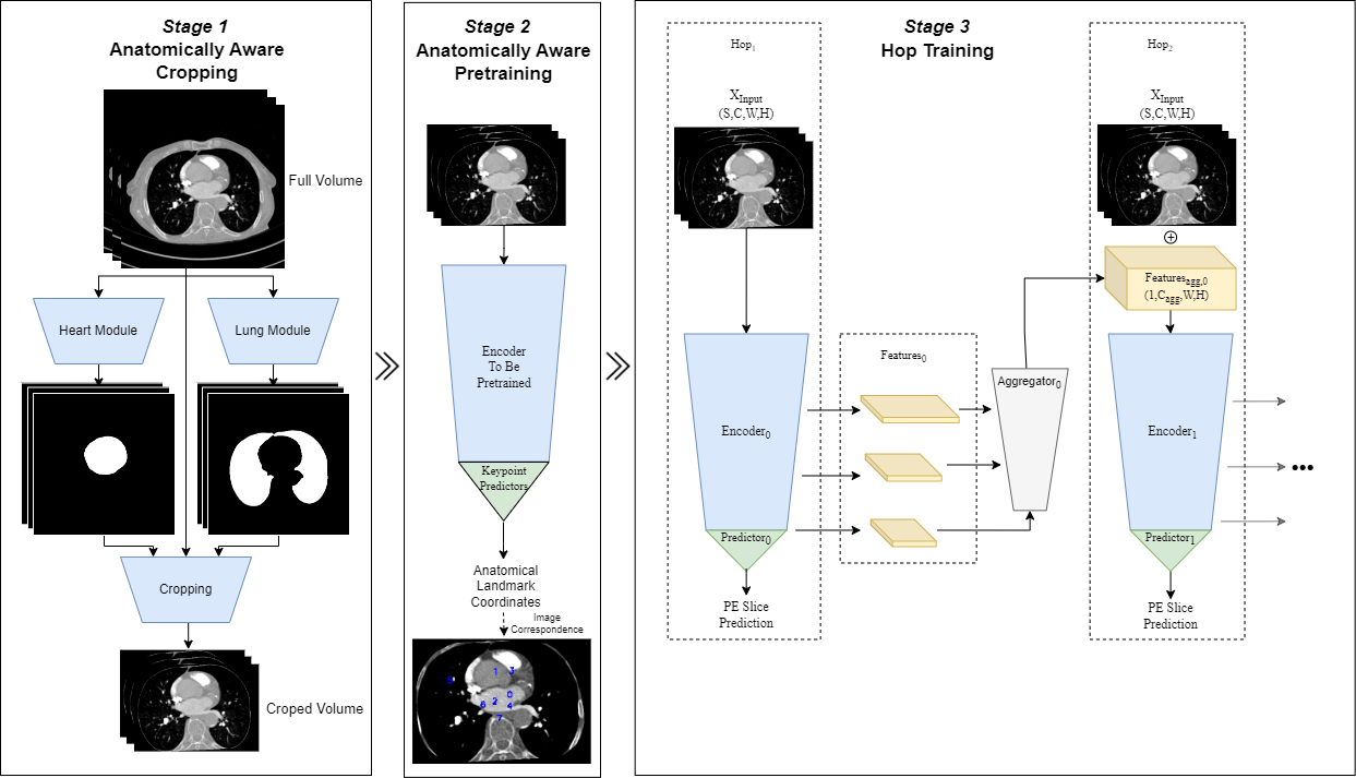
Figure 1: Proposed workflow: each stage represents one of the contributions. Left: Anatomically Aware Segmentation and Cropping, through which data is specialised for PE detection. Middle: Anatomically Aware Pretraining on the related task of Anatomical Landmark Detection, through which the model is primed for our task of Pulmonary Embolism detection. Right Hopped training, through which model predictions are refined, over two hops of neural processing.

Given the need for reducing the workload in hospitals, and the strong previous results obtained by CNNs in the space of disease detection and classification using medical imaging, in this study we design an image processing system, which starts with the detection of specific anatomical structures and continues with a two-phase (initial followed by refined) detection of pulmonary embolisms. Each component in the pipeline is vital for the observed performance, as demonstrated below in the thorough theoretical and experimental analysis and validation.

Main Contributions. We introduce a powerful deep neural architecture for Pulmonary Embolism detection, with state of the art performance, which comprises three different phases, along three independent axes, which prove to be necessary for an accurate performance:

1. First phase: anatomically aware masking and cropping of lung and heart regions. Deep neural modules trained on physiological information for segmenting lung and heart regions, are used to segment only the relevant information with respect to PE detection.

2. Second phase: anatomically aware pretraining. Relevant features are pretrained on the task of localizing specific anatomical keypoints, before starting the PE learning phase.

3. Third Phase: dual-hop architecture for PE detection. The dual-hop architecture allows for a classification in two-stages. The first stage performs an initial evaluation, and the second stage, having access to the initial input as well as the output of the first stage, is able to produce a more accurate, refined prediction.

From an experimental point of view, we show that each component brings an important boost in performance, while the overall system achieves state of the art results compared to the recently published methods.

2 Related work

Pulmonary embolism detection. Previous publications [23, 24, 28, 26, 29, 30, 31, 32, 33, 25, 34] have addressed the task of creating a Computer Assisted Detection (CAD) system for Pulmonary Embolisms (PE), through traditional image processing techniques, based on segmentation and thresholding [30, 33, 32, 31], or through Deep Learning approaches [23, 24, 28, 26, 29, 25, 35], specifically convolutional neural networks (CNNs). Of special interest for comparison with our work are two papers, Weikert et al. [25] and Ma et al. [27]. They both report state of the art performance on large, multi-center datasets.

Weikert et al. [25] present a method reporting state of the art performance on a large dataset, using CNNs. Their method was also evaluated independently by Cheikh et al. [23] and Buls et al. [36] on their own large multicenter datasets. Their methods rely on a two stage CNN trained on 28000 CTPA studies. The evaluation in the original study is done on 1455 studies (positivity rate of 15%), where the model achieves a sensitivity of 92.7%, a specificity of 95.5%, and an F1 score of 86%. Cheikh et al. [23] evaluated the method on 1202 studies (positivity of 15.8%), obtaining similar results, with a sensitivity of 92.6%, a specificity of 95.8%, and an F1 score of 86%. Buls et al. [36] evaluated the method on 500 studies (positivity of 15.8%), obtaining similar results, with a sensitivity of 73%, a specificity of 95%, and an F1 score of 73%.

Ma et al. [27] trains and evaluates, similar to us, on the RSNA dataset [37]. Additionally, they also compare their approach directly with previous work, such as PENet [26], or the Kaggle winning solution of Xu [38] on the same dataset. Their method consists in a two stage pipeline: a local stage in which a 3D model generates a 1D feature sequence based on a neighbourhood of slices, and a global stage in which a sequence model is applied to obtain study level predictions. They report results on both the RSNA [37] official test set, and a holdout validation set, outperforming previous methods reported on the RSNA dataset dataset [37]. The study level PE prediction performance is reported with a sensitivity of 86% sensitivity and a specificity of 85% specificity on the validation set, respectively a sensitivity of 82% and a specificity of 90% specificity on the test set.

The Kaggle challenge for the RSNA dataset [37] also introduced solutions reporting good performance [38, 39, 40, 41], with the difference that they optimize the design for different metrics used in the challenge, such as RV/LV ratio in the case of [39]. Due to this aspect, and because only the aggregated challenge metric was officially reported, a direct comparison with the challenge solutions is difficult.

Segmentation of relevant region of interest. In medical imaging, often only an approximate region of interest from a 3D volume is retained, thus decreasing the computational cost. Such techniques are often also employed to maximize performance, an example being the nonzero region cropping used by the nnUnet framework [42], or the lung based cropping [38, 27].

Pretraining on auxiliary tasks. Transfer learning from pretrained networks has become commonplace, with papers of reference, such as BiT [43], showing robust improvements on the downstream task enabled by using well pretrained models on large datasets. This applies even when the target domain, e.g. medical domain, is very different from the pretraining domain, e.g. natural domain. Other researches show the positive impact of self-supervised learning based pretraining [44, 45, 46], or pretext task learning. [47, 48, 49].

3 Our approach

Our pipeline introduces changes on three orthogonal axes:

1. Preprocessing - anatomically aware masking and cropping of the input: significant boosts in speed and performance are obtained by retaining only task relevant regions of the input.

2. Pretraining - anatomically aware pretraining: priming the model with domain knowledge by learning to predict landmarks of anatomical significance.

3. Architecture - multi-hop architecture: allows for prediction refinement through iterative network forward loops.

Each aspect contributes individually to the performance of the entire pipeline. The improvements brought by each step are additive due to the fact that each change acts on a different dimension of the task. Our proposed pipeline is displayed in Figure 1, offering an overview of each component and their interaction.

Baseline Model. The pulmonary embolism detection task aims, given a 3D input shape (volume of CT slices of a specific width and height), to predict the presence of pulmonary embolism in each slice, resulting in a 1D output (one prediction per slice). Ultimately a study level prediction regarding the presence of PE in the entire volume is performed, by considering all the individual slice outputs.

For the sub-task of predicting the presence of pulmonary embolism at slice level, a 2D CNN is employed, specifically an EfficientNetV2-L [50]. The model is applied in a sliding window fashion on strides of 3 slices, predicting the label of the central slice. Standard Hounsfield Unit (HU) windowing, which normalizes and preserves a targeted intensity range, is applied using 3 windows with their respective proprieties of (window center, window width): [(0,1500),(100,700),(40,400)], obtaining a 3D volume of shape (3, 3, h, w). Similar to Pan et al. [39], the three HU windows are selected to best observe certain tissue types, aiming to maximize relevant information offered to the network. The three windows are targeting lung tissue, pulmonary arteries with contrast, and, respectively, mediastinal tissue. To adjust to the expected input shape of a 2D network, first, two dimensions are flattened, obtaining an input of shape (3*3, h, w).

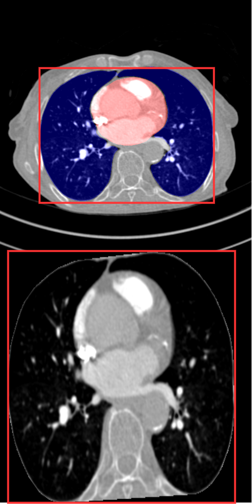
Figure 2: Top: Raw Input central Slice, with the lungs and heart segmentations highlighted in blue, and, respectively, red; Bottom: Full Crop of the central slice. Images are scaled to the same size to better understand intuitively the increase in resolution brought by the cropping mechanism, red borders capture the same anatomical structure. Note that in the cropped image, at a higher resolution, we can observe more structural details that can help for the diagnosis.

We also considered several other highly performant networks, such as Image Transformer [51, 52], ECANet [53], DenseNet [54], CoATNet [55] and RegNet [56], but tests indicated that EfficientNetV2-L is the one best suited for our experiments. We also tested 3D convolutional networks, such as X3D [57] or Resnet3D [58], which operate at the level of the entire 3D volume. Theoretically they are able to better handle 3D volumes, but they produced slightly worse results in our experiments, probably because 3D Conv Nets are best suited for spatio-temporal volumes (e.g. videos).

To obtain the study-level prediction (at the level of the entire CT volume), a simple voting mechanism is applied over the 1D sequence of slice level PE probabilities., noted as $\rho$, predicted by the network $\Theta$ on the entire study.

The voting mechanism outputs positive if more than $\mu_{Study}$ slices are over $\delta_{Slice}$, as in (1). Both parameters are calculated by maximizing the F1 measure on the validation set, as in (2).

$$\pi_{\begin{subarray}{c}\mu_{Study},\\ \delta_{Slice}\end{subarray}}(\rho)=(Count(\rho>\delta_{Slice})\geq\mu_{Study}).$$ (1)

$$\begin{subarray}{c}\mu_{Study},\\ \delta_{Slice}\end{subarray}=\operatorname*{arg\,max}_{\begin{subarray}{c}\mu_{Study},\\ \delta_{Slice}\end{subarray}}\hskip 5.01874pt\underset{S\in Val}{F}\hskip 5.01874pt(\pi{\mu_{Study},\delta_{Slice}}(S),T).$$ (2)

We considered other methods for study level prediction, including sequence modeling models, such as LSTM [59], temporal CNN [60] or transformers [61], as mentioned by other similar publications [35, 38, 27]. The overall performance of more sophisticated approaches was very similar to the much simpler voting mechanism, most probably due to the relatively limited amount of training data (6000 sequences for training). Overall, we preferred the simpler voting scheme due to its transparency and explainability.

All training details are presented in the Section Implementation details.

Anatomically aware masking and cropping. The ability to focus on only the regions that are relevant to PE detection can greatly improve efficiency and accuracy. In our case regions in which Pulmonary Embolisms may manifest are around the location of the lungs, the heart and the pulmonary artery. During the first phase we first detect the lungs and heart masks, using state of the art AI models deployed in many of our products [62], and then obtain a final PE region of interest by taking the convex hull of the individual organ segments. The convex hull helps with filling any possible gaps between masks, to make sure that all possible PE locations are considered at later stages. Note that while the lungs masks would be generally sufficient, the addition of the heart helps cover edge cases such as when one lung is not fully visible, to ensure that the pulmonary artery is still covered by the mask. Various issues can lead to lack of visibility, such as liquid fillings, lung collapse or pneumonectomy,

Anatomically aware pretraining. By pretraining the model on a pretext task [47, 49, 48], the model adapts to the structure of the target domain, i.e., herein Computerized Tomography Pulmonary Angiograms. We take this a step further by using an anatomically driven task, i.e., landmark detection, which primes the model with knowledge of the complex structure of the human body.

By learning the anatomical structure of the lungs, the model ought to be able to localize each structure, and determine its normal appearance. This would make it easier to differentiate areas of interest where PEs occur, such as arteries, from veins or the pleural space.

The anatomical pretraining is framed as a regression problem: the model learns to predict the image coordinates of an anatomical landmark. To compensate for various scan acquisition protocols, resulting in different longitudinal axis displacements, we regress the distance in slices between the current central slice and the target landmark instead of the raw longitudinal coordinate. To generate the ground truth for this task, an internal state of the art model is used [63], detecting up to 20 landmarks.

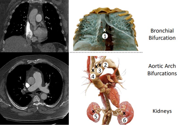
Figure 3: Visualization of a few anatomical landmarks used for our anatomical aware pretranining. On the left we visualize a traversal and a coronal sections of a body 3D-CT scan. On the right we highlight the different anatomical structures and mark the individual landmark points: (1) bronchial bifurcation, (2) bifurcation of left subclavian artery, (3) bifurcation of left common carotid artery and left subclavian artery, (4) bifurcation of left common carotid artery and brachiocephalic artery, (5) center of right kidney, (6) center of left kidney . Courtesy of Florin Ghesu.

The landmarks $\chi$ prediction $K_{o}$ task can be seen as the composition of two functions that need to be learned (3): the 3D homography transformation $H_{s}$ from the initial study view $\nu_{o}$ to a standardized view space $\nu_{s}$ (4), and landmark detection in this standardized space $K_{s}$ (5). We consider that the 3D homography between the two views of two different studies is a powerful concept for the model to learn, and to be able to do so, at least 4 landmarks are required.

$$\begin{split}K_{o}(\nu_{o}).&=\chi.\\ &=K_{s}(H_{s}(\nu_{o})).\end{split}$$ (3)

$$H_{s}(\nu_{o})=\nu_{s}.$$ (4)

$$K_{s}(\nu_{s})=\chi.$$ (5)

To regress coordinates instead of classifying the PE presence, architectural changes were required. A ResNet18 [64] is applied over the unpooled features of the network for each coordinate. This location in the pipeline was selected given its good trade-off between spatial information and the amount of the original encoder that would be trained in the pretraining stage.

Hopped Training.

Given the nature of the task, which aims to detect Pulmonary Embolisms which are often tiny [65, 66], allowing the network to use global context in the earliest layers was considered paramount. While previous work on these lines aimed to capture and use global context throughout the network [67, 68], we opted for a method that refines iteratively the prediction through multiple passes, similar to our previous work on detecting roadmaps in aerial images [69]. The model is composed of two modules, with the same architecture, the two hops. The first module performs an initial prediction, whereas the second module takes as input the original input together with the output of the initial module, to refine the prediction. The two are combined and trained together end-to-end, such that each module learns its own set of network weights. A related but more distant approach [70] was also proposed in the context of signal processing, where the output of the previous stage along with the initial input is passed through the exact same net, having the exact same parameters, for several iterations.

$$\tau_{n},\psi_{n+1}=\Theta(input,\psi_{n}).$$ (6)

Similarly to the methods described above, we design a method that refines its prediction iteratively based on features from previous passes. We hypothesize each hop generates a richer context embedding, allowing the following Hops to focus on finer details.

The model in each hop is noted as $Theta_{k}$. The architecture in each hop can be different if desired, allowing for creative assembling. We take advantage of this by initializing and freezing $hop_{0}$ with an already trained network on the task, and only training $hop_{1}$ with the minimal overhead, when compared to training a no hop pipeline.

In our 3D context, a reformulation was required for the obtained features to match the input size. Inspired by UNET [15], our pipeline aggregates and processes feature maps from various levels of the previous pass, $\psi_{agg,n}$. The resulting feature map has the same width and height as the input, allowing for the straight forward concatenation to the input in the second hop. This aggregation takes process in a simple network for each hop K, $\phi_{k}$. Our formulation takes the form of eq. (7)

$$\tau_{1},\psi_{1}=\Theta_{1}(input).\\$$ (7)

$$\psi_{agg,n}=\Phi_{n-1}(\psi_{n-1}).\\$$

$$\tau_{n},\psi_{n}=\Theta_{n}(input,\psi_{agg,n}).\\$$

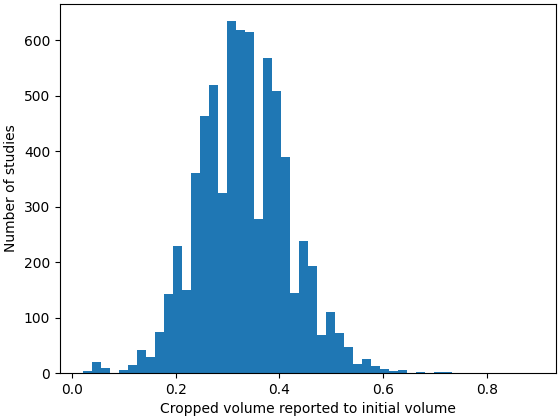
Figure 4: Distribution of ratios between the volume of cropping using the lung and heart study, and the original study. On average, the cropped volume represents only 34% of the initial volume, and in some instances only 15% of the initial volume.

4 Implementation Details

Baseline Architecture. The neural network model used herein was EfficientNetV2-L [50], imported from the Timm library [71], using random initialization based on He initialization [72], respectivelly using the ImageNet21K [73] pretrained model. For pretrained models, the last linear layer is replaced with a layer outputting two classes.

The training was performed using the LARS optimizer [74], with a learning rate of 0.003, a 1000 step linear warmup, and a linear decay learning rate scheduler over 10 epochs. The standard multiclass cross entropy loss was used.

HU windowing was applied on the data, with 3 (center, width) windows: pulmonary specific window of (100,700), soft tissue window of (40,400) and lung tissue window of (-600,1500). Images are resized to a size of (576,576) using bilinear interpolation.

During training several augmentations are used, applied on each slice using the same parameters. The Albumentation [75] library was used, and augmentation were applied in the following order with said parameterization:

⬇

RandomContrast(limit=0.2, p=1.0)

ShiftScaleRotate(shift_limit=0.2, scale_limit=0.2,

rotate_limit=45, p=1.0)

Cutout(num_holes=2, max_h_size=0.4*576,

max_w_size=0.4*576, fill_value=0, p=1.0)

While the Cutout augmentation is counter intuitive, since it may cover the only PE in the image, it still seems to work well, probably due to forcing the model to rely on secondary, uncovered PEs. In positive cases, it is common for multiple PEs to be present [76], and, as observed in Figure 8, our model captures multiple emboli, indicating robustness to possible imaging issues making the primary embolism unobservable.

Input Cropping. The segmentation mask for cropping the region of interest was composed of lungs masks [LungDetector] and heart masks [HeartDetector], generated using internal models. Masks are combined and a convex hull is applied over them, on each slice independently, using open-cv [77], to fill any possible gaps between masks.

Keypoint pretraining. The training was performed using the SGD optimizer [78], with a learning rate of 0.1, a 1000 step linear warmup and a linear decay learning rate scheduler over 10 epochs. The mean squared error loss was used. Keypoints corresponding to axes X and Y are normalized to the [0,1] range using image dimensions, and Z is transformed as a relative distance from the current middle slice, then normalized to [0,1] by dividing by 600, which is an upper limit of slice count in the RSNA training dataset [37]. Keypoints used in the pretraining process are: Heart, Carina Bifurcation, T4, Right Primary Bronchus, Aortic Arch Center, Aortic Root, Left Subclavian Artery, Left Primary Bronchus, Left Common Carotid Artery, Liver Top, Right Medial Clavicle, Suprasternal Notch, Brachiocephalic Artery Bifurcation, Left Medial Clavicle, Right Subclavian and Vertebralis Branch, Left Subclavian and Vertebralis, Right Lung Top, Sternum Tip, Left Lung Top, Celiac Trunk.

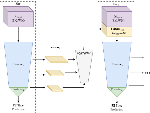
Figure 5: Hop Training, illustrated for $Hop_{1}$ and $Hop_{2}$. The model from $Hop_{1}$ receives as input only the 3D slice volume $X_{input}$, while the following $Hop_{2}$ receives an additional $psi_{1}$, corresponding to the aggregated features from $Hop_{1}$.

Hop Training. Hop Training at step K is represented by two parts, $Aggregator_{K}$ and $Encoder_{K}$. The $Aggregator_{K}$ upsamples feature maps obtained from the previous $Encoder_{K-1}$, and is composed of 6 upsample blocks as described bellow, with respective channels, from bottom up [1280,224,96,64,32,9], corresponding to extracted features from the $Encoder_{k-1}$:

⬇

Sequential(Conv2d(in_ch, mid_ch, 3, 1),

BatchNorm2d(mid_ch),

ReLU(),

Conv2d(mid_ch, out_ch, 3, 1),

BatchNorm2d(out_ch),

ReLU(),

Upsample(scale_factor=2, mode=’bilinear’))

After upsampling, the obtained features are concatenated to the corresponding $Encoder_{k-1}$ features, then passed to the next upsample module.

The $Encoder_{K}$ is built as in Basic Architecture, the only difference is that the first convolution has input channels equal to the input channels plus the concatenated channels, in our case 9 and 9.

For our 1 Hop experiment, we initialized both Encoders with the best weights from the previous experiments, we froze $Encoder_{1}$, and then retrained $Encoder_{2}$ as described in Basic Architecture.

5 Experimental Analysis

In our experiments, we aimed to demonstrate the impact of each of the proposed improvements separately, as well as the improvement brought by their combined usage.

5.1 Datasets

We performed experiments on the publicly available RSNA dataset [37]. The RSNA dataset acted as a training and validation dataset, opting for a larger, more representative validation set instead of two smaller validation and test set. Ablations studies and final performance are all reported on the validation set.

The public RSNA dataset contains approximately 7200 studies (CT scan volumes), with slice level annotations regarding the presence of a pulmonary embolism, and several study level annotations. For further details, see the dataset paper [37]. Out of 7200 studies, approximately 400 were excluded since the segmentation models [62] were not able to detect the lungs or heart. A similar rate of case exclusion of 10.4% is reported by Buls et al. [36] for the model based on Weikert et al. [25, 23].

Additionally, 14 studies that were marked as indeterminate as per [37] were excluded from the validation set. The final train/validation split was 6000/836 cases.

Data split, including what cases were excluded due to study quality issues will be released as well for reproducibility purposes.

5.2 Anatomical aware cropping

To study the impact of the cropping process, an ablation study was performed. Of interest for this study were experiments using the following cropping styles:

1. Uncropped image, acting as a baseline for our evaluation.

2. Crop using the segmentations of lungs and heart. This was considered to be the best crop, capturing all regions in which pulmonary embolisms could manifest.

The results are presented in Table 1.

Cropping Type	Sens	Spec	PPV	NPV	F1	Volume
Original Slice	0.920	0.944	0.852	0.971	0.884	100%
Cropped Slice	0.958	0.933	0.832	0.984	0.890	34%

Table 1: Results for different types of input preprocessing, as presented in Figure 2. Cropped slice leads to significant improvements in terms of F1 score, trading specificity and PPV for sensitivty and NPV.

Our intuition is that performance improvements are brought by two changes to the nature of the input:

1. Eliminating anatomical structures (e.g., liver and ribs) in which pulmonary embolism cannot be present, but still are proximal to the areas of interest, which could require additional expressiveness to rule out. Such anatomical structures could act as distractors, therefore removing them from the input images should be beneficial.

2. Lowering the size of the image by removing background space and clutter, focus on the relevant areas only and allow for greater resolution of such areas of interest (e.g., lungs), while keeping the size of the network input the same. In CTPAs, on average 34%, up to 80% of the image can be background space, as illustrated in Table 1, respectively Figure 4. While our pipeline takes as input the entire image, resized to a fixed input size, we expect our anatomical cropping preprocessing to be compatible when using popular cropping augmentations as well, since it ensures more salient, non-background crops.

Since the cropping process results in different image sizes for each study, the cropping output is resized to a fixed size before being fed into the pipeline, to allow for batch training. This restriction allows us to only evaluate the gain in performance that can be obtained by using more salient images, and not the potential speedups. While different proxies could have been used to measure speed up, classification performance maximization was the focus of our work.

5.3 Anatomically aware pretraining

In this section, we analyze the impact of the initial weights of the neural network, when starting the PE detection training. For a better evaluation of our method, we decided to evaluate against two baseline initializations:

1. Random initialization, using He initialization [72]. Standard initialization, representing a lower bound of performance, and a weak baseline.

2. Imagenet-21K [73] pretrained model, imported from the Timm library [71]. As shown in BiT [43], pretraining on natural images can significantly improve performance of a model even when shifting the task to recognition in the medical domain. We consider this as a strong baseline.

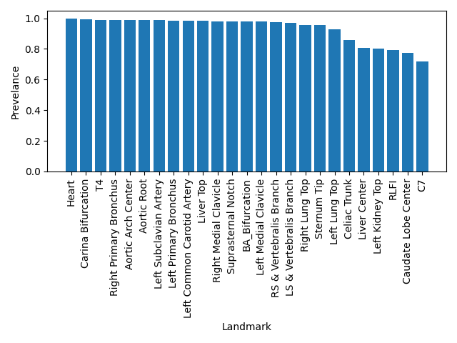
Figure 6: Presence of landmarks as percentage of total studies. 20 landmarks were considered to be a good trade-off between number of studies and expressiveness of the pretraining task.

Comparing the two baselines is valuable since it allows us to better understand the importance of pretraining, even when performed on very different domains. Most relevant research operate on small datasets, whereas showing the benefit of pretraining in the large data regime is essential in light of large datasets emerging in the medical AI space [37, 79].

Experiment Name	Sens	Spec	PPV	NPV	F1
Baseline + Anatomical Crop
Random Init	0.693	0.727	0.468	0.873	0.559
+ Imagenet21K Initialization
Imagenet21K Init	0.958	0.933	0.832	0.984	0.890
+ Anatomical Pretraining
Localization Pretrained	0.934	0.946	0.857	0.976	0.894

Table 2: Results obtained by models starting from different initial weights. The comparison is performed between models starting from ”Random initialization” based on He [72], the ”Imagenet-21K Pretrained” model imported from Timm [71], and our ”Localization Pretrained” model. Our initialization obtains an increase in performance even when compared with a strong baseline such as Imagenet-21K Pretraining.

Our localization pretraining is performed by learning to regress 20 anatomical landmarks, listed in the implementation details. These landmarks were detected using a state-of-the-art model [63] and were selected based on their prevalence in the data. The aim was to use as many landmarks as possible, while maximizing the number of usable studies. The landmarks are only necessary in the pretraining phase, so this does not impact the number of studies available for the final training. While 4 3D points would have been sufficient to determine the 3D homography, the use of additional 16 landmarks compensates for the detection noise [80], allowing the network to learn a more stable representation of the 3D homography from the current study to the standardized view.

To maximize performance, we start from the already powerful Imagenet-21K pretrained weights, aiming to demonstrate that the model can be further improved for our task.

Figure 6 displays for various landmarks the percentage of studies that contain those landmarks. We opted for the use of the top 20 most present landmarks. In the case of strongly correlated groups of keypoints, such as the vertebrae, a single landmark has been selected.

As shown in Table 2, our type of anatomically aware pretraining outperforms the strong baseline set by pretraining on Imagenet-21K [73]. Models use the Full Crop preprocessing step, to maximize performance.

We also show that even when using as starting point models pretrained on natural images, such as the ones in ImageNet21K [73], an important boost in performance is observed when refining on medical imaging. This reinforces the generability of such models, as shown in BiT [43].

5.4 Dual-Hop Architecture

In this section we analyze the performance boost determined by adding an additional hop. First hop is initialized and frozen using the best weights from the previous section 5.3. Experiments were limited to two hops.

In table 3 a quantitative comparison between the two hops on the RSNA dataset [37] is presented: the second hop leads to an improvement of 1.6% in the F1 score. In Figure 7 a comparison between slice level probabilities is illustrated: $Hop_{1}$ displays a slightly more stable curve, while also capturing an additional PE in subplot B, missed by the initial pass.

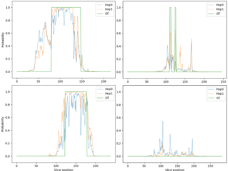
Figure 7: Samples of slice level probability predictions, plotted as a signal over the entire study. Probabilities generated by $Hop_{0}$ are displayed in blue, in orange for $Hop_{1}$, and in green for the $GroundTruth$. The signal generated by $Hop_{1}$ is slightly more stable, also detecting tiny PEs missed by the $Hop_{0}$ in subplot B

Hop Index	Sensitivity	Specificity	PPV	NPV	F1
Hop 1	0.934	0.946	0.857	0.976	0.894
Hop 2	0.929	0.961	0.891	0.975	0.910

Table 3: Multi Hop Training Results. The second Hop leads to a performance boost.

The conclusion of these experiments is that by adding the second hop, for which a different set of weights is learned, and which has access to both the original input and the output of the first hop, we are able to better focus on details (missed by the initial hop) which are relevant in the hard cases.

5.5 Full pipeline

The performance of the final pipeline achieves results in the state-of-the-art range, and are similar to the average performance of radiologists, which have reported a sensitivity between 0.67 and 0.87 and a specificity between 0.89 and 0.99 [81, 82, 83, 24]. We compare our results to the state of the art solution evaluated in two different studies [25, 23]. The second study also benchmarks the performance of radiologists on the same dataset, see table 4.

Although different datasets are used, and a direct comparison is not possible, compared to radiologist performance reported by Cheikh et al. [23], our performance is slightly worse in terms of F1 score, with a larger drop of 6% in PPV, but a gain of 3% in sensitivity. Given the target application of triage, such a trade-off ought to work well, as noted by other studies [23], since positives would also be reviewed by a physician.

We also compare the results with those of an approach evaluated on the RSNA dataset [37], although on a different data split.

The performance of Wa et al. [27] for study level PE prediction, presented in Table 4, is slightly lower. However, they report better performance in terms of AUROC than PENet [26], and the Kaggle 1st place [38]. While, at a high level, their method is similar to out baseline model, it uses a smaller network, 3D Resnet18 [64, 58], and a smaller input size. Another difference is that they optimize for multiple tasks.

Model	Sens	Spec	PPV	NPV	F1
Weiker [25] AI Model	0.927	0.955	0.796	0.986	0.860
Cheikh [23] AI Model	0.926	0.958	0.804	0.986	0.861
Cheikh [23] Radiologist	0.9	0.991	0.95	0.981	0.924
Buls [36] AI model	0.73	0.95	0.73	0.94	0.73
Ma [27] on RSNA val	0.86	0.85	-	-	-
Ma [27] on RSNA test	0.81	0.90	-	-	-
Our baseline model	0.920	0.944	0.852	0.971	0.884
+ Cropping	0.958	0.933	0.832	0.984	0.890
+ Pretraining	0.934	0.946	0.857	0.976	0.894
+ Hop ( Our final model )	0.929	0.961	0.891	0.975	0.910

Table 4: Comparison of results with state of the art solutions [23, 25, 36] and Ma [27] on the RSNA dataset [37]. Our model, compared to state of the art [23, 25, 36], obtains better results in terms of F1 score and PPV, and performs similarly in terms of sensitivity, specificity, and NPV. Our model performs slightly worse when compared to a human radiologist. Compared to Ma [27] on the RSNA dataset, significantly better results are obtained.

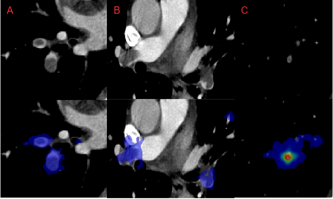
Figure 8: Samples of model feature use generated using Integrated Gradients [84]; all three samples are predicted as positive. The model uses the presence of PEs as the main information source. Figure A (left) displays two clear PEs captured by the model. Figure B (middle) displays 3 distinct distant PEs, indicating the capability of extracting information from multiple sources. Figure C (right) displays a hard case of a small subsegmental PE captured by the model.

5.6 Model feature use

An key aspect of applying deep learning models in the real world is model explainability. Hence, an important factor is feature use visualization, allowing one to determine, for each example, major contributors for the final prediction. This is especially important for the deployment in the medical domain, where spurious correlations may appear due to the data acquisition protocol [85, 86].

For our models we analyzed the feature use generated using the integrated gradients algorithm [84], implemented in the Captum library [87]. A couple of examples from the RSNA dataset [37] are displayed in Figure 8, indicating that the model uses the present PEs as primary source of information.

5.7 Error Analysis

Model error analysis, especially from a clinical perspective, is a critical part of an medical AI model. Our final model makes 39 erros, of which 24 False Positives and 15 False Negatives. Examples are shown in Figure 9.

Similar to other methods [23, 25], our False Positives are caused by contrast agent related flow artifacts. Another cause is the presence of other pathologies such as pulmonary metastases or granulomas. Such cases are displayed on the right side of Figure 9.

In the case of False Negatives, the main factor was the dimension of the PE, most missed cases containing tiny and subsegmental PEs. Such cases are displayed on the left side of Figure 9.

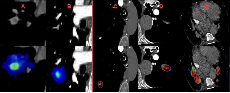
Figure 9: Error analysis. A and B display False Negative cases, in which the model pays attention to PEs, but lacks confidence. In A the contrast quality is suboptimal, and B displays a tiny PE which was missed. C, D and E display False Positives: C was caused by a calcified granuloma, D by a mucous plugging, and E by very low image quality. The top row displays the original input, windowed to the PE specific range, the bottom row displays model prediction feature use.

6 Conclusion

In this paper we presented three mechanisms through which an automatic system for CT pulmonary embolism detection can be improved. The three orthogonal dimensions of processing and learning from the CT data, correspond to phases, which progressively address the initial anatomically aware segmentation of the regions of interest, followed by the pretraining of the classification module on the adjacent task of detecting anatomical landmarks, and finally by the task of pulmonary embolism detection, for which we propose a dual-hop process. These phases, in essence, follow the intuitive normal steps in which a doctor performs the diagnosis based on medical images: focus of attention on the region of interest, use of rich previously learned knowledge of anatomy, followed by a rigorous pathological examination during several cycles of inspection at different levels of detail. Our extensive experiments demonstrate the effectiveness of each of these phases. However, besides the demonstrated results on a specific and highly important medical problem, the three mechanisms introduced in this paper also constitute a more general proof of concept, which could open the door for similar approaches in other medical analysis tasks.

Another special added value of our work, for the medical AI community, are the significant quantitative improvements over strong baselines and state of the art, in the big data regime. These significant improvements are brought by each of our contributions to the proposed pipeline: anatomically aware cropping, pretraining on pretext tasks, as well as a dual hop architecture for the final classification. While each of these components is related to different works which are not related to the medical field, ours is the first to bring them together, in a novel and original way, to produce significant improvements in the field of pulmonary embolism detection.

Disclaimer: The concepts and information presented in this paper/presentation are based on research results that are not commercially available. Future commercial availability cannot be guaranteed.

References

- [1] G. E. e. a. Raskob, “Thrombosis: a major contributor to global disease burden,” Arteriosclerosis, thrombosis, and vascular biology, vol. 34, no. 11, pp. 2363–2371, 2014.
- [2] K. e. a. Keller, “Trends in thrombolytic treatment and outcomes of acute pulmonary embolism in germany,” European heart journal, vol. 41, no. 4, pp. 522–529, 2020.
- [3] A. M. Wendelboe and G. E. Raskob, “Global burden of thrombosis: epidemiologic aspects,” Circulation research, vol. 118, no. 9, pp. 1340–1347, 2016.
- [4] I. K. et al., “Risks of deep vein thrombosis, pulmonary embolism, and bleeding after covid-19: nationwide self-controlled cases series and matched cohort study,” BMJ, vol. 377, p. e069590, 4 2022.
- [5] P. Lehnert, T. Lange, C. H. Møller, P. S. Olsen, and J. Carlsen, “Acute pulmonary embolism in a national danish cohort: increasing incidence and decreasing mortality,” Thrombosis and haemostasis, vol. 118, no. 03, pp. 539–546, 2018.
- [6] F. Dentali, W. Ageno, F. Pomero, L. Fenoglio, A. Squizzato, and M. Bonzini, “Time trends and case fatality rate of in-hospital treated pulmonary embolism during 11 years of observation in northwestern italy,” Thrombosis and haemostasis, vol. 115, no. 02, pp. 399–405, 2016.
- [7] J. e. a. de Miguel-Díez, “Trends in hospital admissions for pulmonary embolism in spain from 2002 to 2011,” European Respiratory Journal, vol. 44, no. 4, pp. 942–950, 2014.
- [8] A. T. e. a. Cohen, “Venous thromboembolism (vte) in europe,” Thrombosis and haemostasis, vol. 98, no. 10, pp. 756–764, 2007.
- [9] K. E. Kocher, W. J. Meurer, R. Fazel, P. A. Scott, H. M. Krumholz, and B. K. Nallamothu, “National trends in use of computed tomography in the emergency department,” Annals of emergency medicine, vol. 58, no. 5, pp. 452–462, 2011.
- [10] I. Portoghese, M. Galletta, R. C. Coppola, G. Finco, and M. Campagna, “Burnout and workload among health care workers: the moderating role of job control,” Safety and health at work, vol. 5, no. 3, pp. 152–157, 2014.
- [11] S. A. Oldham et al., “Ctpa as the gold standard for the diagnosis of pulmonary embolism,” International Journal of Computer Assisted Radiology and Surgery, vol. 6, no. 4, pp. 557–563, 2011.
- [12] Y. LeCun, L. Bottou, Y. Bengio, and P. Haffner, “Gradient-based learning applied to document recognition,” Proceedings of the IEEE, vol. 86, no. 11, pp. 2278–2324, 1998.
- [13] A. Krizhevsky, I. Sutskever, and G. E. Hinton, “Imagenet classification with deep convolutional neural networks,” Communications of the ACM, vol. 60, no. 6, pp. 84–90, 2017.
- [14] K. Simonyan and A. Zisserman, “Very deep convolutional networks for large-scale image recognition,” pp. 1–14, Computational and Biological Learning Society, 2015.
- [15] O. Ronneberger, P. Fischer, and T. Brox, “U-net: Convolutional networks for biomedical image segmentation,” in International Conference on Medical image computing and computer-assisted intervention, pp. 234–241, Springer, 2015.
- [16] T. T. e. a. Ho, “A 3d-cnn model with ct-based parametric response mapping for classifying copd subjects,” Scientific Reports, vol. 11, no. 1, pp. 1–12, 2021.
- [17] M. Polsinelli, L. Cinque, and G. Placidi, “A light cnn for detecting covid-19 from ct scans of the chest,” Pattern recognition letters, vol. 140, pp. 95–100, 2020.
- [18] L. M. e. a. Prevedello, “Automated critical test findings identification and online notification system using artificial intelligence in imaging,” Radiology, vol. 285, no. 3, pp. 923–931, 2017.
- [19] S. Soffer, A. Ben-Cohen, O. Shimon, M. M. Amitai, H. Greenspan, and E. Klang, “Convolutional neural networks for radiologic images: a radiologist’s guide,” Radiology, vol. 290, no. 3, pp. 590–606, 2019.
- [20] R. Yamashita, M. Nishio, R. K. G. Do, and K. Togashi, “Convolutional neural networks: an overview and application in radiology,” Insights into imaging, vol. 9, no. 4, pp. 611–629, 2018.
- [21] H. M. Ali, M. S. Kaiser, and M. Mahmud, “Application of convolutional neural network in segmenting brain regions from mri data,” in International conference on brain informatics, pp. 136–146, Springer, 2019.
- [22] W. e. a. Lin, “Convolutional neural networks-based mri image analysis for the alzheimer’s disease prediction from mild cognitive impairment,” Frontiers in neuroscience, vol. 12, p. 777, 2018.
- [23] A. B. C. et al., “How artificial intelligence improves radiological interpretation in suspected pulmonary embolism,” European Radiology, pp. 1–12, 3 2022.
- [24] S. S. et al., “Deep learning for pulmonary embolism detection on computed tomography pulmonary angiogram: a systematic review and meta-analysis,” Scientific Reports 2021 11:1, vol. 11, pp. 1–8, 8 2021.
- [25] T. W. et al. European radiology, pp. 6545–6553, 12.
- [26] S. C. H. et al., “Penet—a scalable deep-learning model for automated diagnosis of pulmonary embolism using volumetric ct imaging,” npj Digital Medicine 2020 3:1, vol. 3, pp. 1–9, 4 2020.
- [27] X. Ma, E. C. Ferguson, X. Jiang, S. I. Savitz, and S. Shams, “A multitask deep learning approach for pulmonary embolism detection and identification,” Scientific Reports 2022 12:1, vol. 12, pp. 1–11, 7 2022.
- [28] W. L. et al., “Evaluation of acute pulmonary embolism and clot burden on ctpa with deep learning,” European Radiology 2020 30:6, vol. 30, pp. 3567–3575, 2 2020.
- [29] S. C. Huang, A. Pareek, R. Zamanian, I. Banerjee, and M. P. Lungren, “Multimodal fusion with deep neural networks for leveraging ct imaging and electronic health record: a case-study in pulmonary embolism detection,” Scientific Reports 2020 10:1, vol. 10, pp. 1–9, 12 2020.
- [30] C. Z. et al., “Computer-aided detection of pulmonary embolism in computed tomographic pulmonary angiography (ctpa): Performance evaluation with independent data sets,” Medical Physics, vol. 36, p. 3385, 2009.
- [31] J. Liang and J. Bi, “Computer aided detection of pulmonary embolism with tobogganing and mutiple instance classification in ct pulmonary angiography,” Information processing in medical imaging : proceedings of the … conference, vol. 20, pp. 630–641, 2007.
- [32] E. Pichon, C. L. Novak, A. P. Kiraly, and D. P. Naidich, “A novel method for pulmonary emboli visualization from high-resolution ct images,” Medical Imaging 2004: Visualization, Image-Guided Procedures, and Display, vol. 5367, p. 161, 5 2004.
- [33] H. Bouma, J. J. Sonnemans, A. Vilanova, and F. A. Gerritsen, “Automatic detection of pulmonary embolism in cta images,” IEEE Transactions on Medical Imaging, vol. 28, pp. 1223–1230, 8 2009.
- [34] K. Mueller-Peltzer, L. Kretzschmar, G. N. de Figueiredo, A. Crispin, R. Stahl, F. Bamberg, and C. G. Trumm, “Present limitations of artificial intelligence in the emergency setting–performance study of a commercial, computer-aided detection algorithm for pulmonary embolism,” in RöFo-Fortschritte auf dem Gebiet der Röntgenstrahlen und der bildgebenden Verfahren, vol. 193, pp. 1436–1444, Georg Thieme Verlag KG, 2021.
- [35] S. Suman, G. Singh, N. Sakla, R. Gattu, J. Green, T. Phatak, D. Samaras, and P. Prasanna, “Attention based cnn-lstm network for pulmonary embolism prediction on chest computed tomography pulmonary angiograms,”
- [36] N. Buls, N. Watté, K. Nieboer, B. Ilsen, and J. de Mey, “Performance of an artificial intelligence tool with real-time clinical workflow integration–detection of intracranial hemorrhage and pulmonary embolism,” Physica Medica: European Journal of Medical Physics, vol. 83, pp. 154–160, 2021.
- [37] E. e. a. Colak, “The rsna pulmonary embolism ct dataset,” Radiology: Artificial Intelligence, vol. 3, no. 2, p. e200254, 2021. PMID: 33937862.
- [38] X. Guanshuo, “1st place solution,” Apr 2018.
- [39] I. Pan, “Deep learning for pulmonary embolism detection: Tackling the rsna 2020 ai challenge,” Radiology: Artificial Intelligence, vol. 3, no. 5, 2021.
- [40] N. Thanh Dat, “Rsna str pulmonary embolism detection,” 2020.
- [41] H. Darragh, “Rsna str pulmonary embolism detection,” 2020.
- [42] F. Isensee, P. F. Jaeger, S. A. A. Kohl, J. Petersen, and K. H. Maier-Hein, “Automated design of deep learning methods for biomedical image segmentation,”
- [43] A. e. a. Kolesnikov, “Big transfer (bit): General visual representation learning,” in European conference on computer vision, pp. 491–507, Springer, 2020.
- [44] F. C. G. et al., “Self-supervised learning from 100 million medical images,” 1 2022.
- [45] P. G. et al., “Self-supervised pretraining of visual features in the wild,” 3 2021.
- [46] T. Chen, S. Kornblith, M. Norouzi, and G. Hinton, “A simple framework for contrastive learning of visual representations,” in International conference on machine learning, pp. 1597–1607, PMLR, 2020.
- [47] C. Doersch, A. Gupta, and A. A. Efros, “Unsupervised visual representation learning by context prediction,” 2016.
- [48] M. Noroozi and P. Favaro, “Unsupervised learning of visual representations by solving jigsaw puzzles,” 2017.
- [49] S. Gidaris, P. Singh, and N. Komodakis, “Unsupervised representation learning by predicting image rotations,” 2018.
- [50] M. Tan and Q. Le, “Efficientnetv2: Smaller models and faster training,” in International Conference on Machine Learning, pp. 10096–10106, PMLR, 2021.
- [51] A. e. a. Dosovitskiy, “An image is worth 16x16 words: Transformers for image recognition at scale,” arXiv preprint arXiv:2010.11929, 2020.
- [52] H. Touvron, M. Cord, A. Sablayrolles, G. Synnaeve, and H. Jégou, “Going deeper with image transformers,” in Proceedings of the IEEE/CVF International Conference on Computer Vision, pp. 32–42, 2021.
- [53] Q. Wang, B. Wu, P. Zhu, P. Li, W. Zuo, and Q. Hu, “Supplementary material for ‘eca-net: Efficient channel attention for deep convolutional neural networks,” in Proceedings of the 2020 IEEE/CVF Conference on Computer Vision and Pattern Recognition, IEEE, Seattle, WA, USA, pp. 13–19, 2020.
- [54] G. Huang, Z. Liu, L. Van Der Maaten, and K. Q. Weinberger, “Densely connected convolutional networks,” in Proceedings of the IEEE conference on computer vision and pattern recognition, pp. 4700–4708, 2017.
- [55] Z. Dai, H. Liu, Q. V. Le, and M. Tan, “Coatnet: Marrying convolution and attention for all data sizes,” Advances in Neural Information Processing Systems, vol. 34, pp. 3965–3977, 2021.
- [56] J. Xu, Y. Pan, X. Pan, S. Hoi, Z. Yi, and Z. Xu, “Regnet: self-regulated network for image classification,” IEEE Transactions on Neural Networks and Learning Systems, 2022.
- [57] C. Feichtenhofer, “X3d: Expanding architectures for efficient video recognition,” in Proceedings of the IEEE/CVF Conference on Computer Vision and Pattern Recognition, pp. 203–213, 2020.
- [58] H. Kataoka, T. Wakamiya, K. Hara, and Y. Satoh, “Would mega-scale datasets further enhance spatiotemporal 3d cnns?,” arXiv preprint arXiv:2004.04968, 2020.
- [59] S. Hochreiter and J. Schmidhuber, “Long short-term memory,” Neural computation, vol. 9, no. 8, pp. 1735–1780, 1997.
- [60] C. Lea, R. Vidal, A. Reiter, and G. D. Hager, “Temporal convolutional networks: A unified approach to action segmentation,” in European conference on computer vision, pp. 47–54, Springer, 2016.
- [61] A. e. a. Vaswani, “Attention is all you need,” Advances in neural information processing systems, vol. 30, 2017.
- [62] J. e. a. Chamberlin, “Automated detection of lung nodules and coronary artery calcium using artificial intelligence on low-dose ct scans for lung cancer screening: accuracy and prognostic value,” BMC medicine, vol. 19, no. 1, pp. 1–14, 2021.
- [63] F.-C. e. a. Ghesu, “Multi-scale deep reinforcement learning for real-time 3d-landmark detection in ct scans,” IEEE transactions on pattern analysis and machine intelligence, vol. 41, no. 1, pp. 176–189, 2017.
- [64] K. He, X. Zhang, S. Ren, and J. Sun, “Deep residual learning for image recognition,” 2015.
- [65] D. C. Diffin, J. R. Leyendecker, S. P. Johnson, R. J. Zucker, and P. J. Grebe, “Effect of anatomic distribution of pulmonary emboli on interobserver agreement in the interpretation of pulmonary angiography.,” AJR. American journal of roentgenology, vol. 171, no. 4, pp. 1085–1089, 1998.
- [66] P. D. Stein, J. W. Henry, and A. Gottschalk, “Reassessment of pulmonary angiography for the diagnosis of pulmonary embolism: relation of interpreter agreement to the order of the involved pulmonary arterial branch,” Radiology, vol. 210, no. 3, pp. 689–691, 1999.
- [67] J. Hu, L. Shen, and G. Sun, “Squeeze-and-excitation networks,” in Proceedings of the IEEE Conference on Computer Vision and Pattern Recognition (CVPR), June 2018.
- [68] Y. Cao, J. Xu, S. Lin, F. Wei, and H. Hu, “Global context networks,” CoRR, vol. abs/2012.13375, 2020.
- [69] D. Costea, A. Marcu, E. Slusanschi, and M. Leordeanu, “Creating roadmaps in aerial images with generative adversarial networks and smoothing-based optimization,” in Proceedings of the IEEE International Conference on Computer Vision Workshops, pp. 2100–2109, 2017.
- [70] A. Banino, J. Balaguer, and C. Blundell, “Pondernet: Learning to ponder,” arXiv preprint arXiv:2107.05407, 2021.
- [71] R. Wightman, “Pytorch image models.” \urlhttps://github.com/rwightman/pytorch-image-models, 2019.
- [72] K. He, X. Zhang, S. Ren, and J. Sun, “Delving deep into rectifiers: Surpassing human-level performance on imagenet classification,” in Proceedings of the IEEE international conference on computer vision, pp. 1026–1034, 2015.
- [73] T. Ridnik, E. Ben-Baruch, A. Noy, and L. Zelnik-Manor, “Imagenet-21k pretraining for the masses,” arXiv preprint arXiv:2104.10972, 2021.
- [74] Y. You, I. Gitman, and B. Ginsburg, “Large batch training of convolutional networks,” arXiv preprint arXiv:1708.03888, 2017.
- [75] A. e. a. Buslaev, “Albumentations: Fast and flexible image augmentations,” Information, vol. 11, no. 2, 2020.
- [76] P. Rali, M. Rali, and M. Sockrider, “Pulmonary embolism part 1,” American journal of respiratory and critical care medicine, vol. 197, no. 9, pp. P15–P16, 2018.
- [77] G. Bradski, “The OpenCV Library,” Dr. Dobb’s Journal of Software Tools, 2000.
- [78] S. Ruder, “An overview of gradient descent optimization algorithms,” arXiv preprint arXiv:1609.04747, 2016.
- [79] U. e. a. Baid, “The rsna-asnr-miccai brats 2021 benchmark on brain tumor segmentation and radiogenomic classification,” arXiv preprint arXiv:2107.02314, 2021.
- [80] R. I. Hartley and A. Zisserman, Multiple View Geometry in Computer Vision. Cambridge University Press, ISBN: 0521540518, second ed., 2004.
- [81] J. e. a. Eng, “Accuracy of ct in the diagnosis of pulmonary embolism: a systematic literature review,” American Journal of Roentgenology, vol. 183, no. 6, pp. 1819–1827, 2004.
- [82] M. e. a. Das, “Computer-aided detection of pulmonary embolism: influence on radiologists’ detection performance with respect to vessel segments,” European radiology, vol. 18, no. 7, pp. 1350–1355, 2008.
- [83] S. J. Kligerman, J. W. Mitchell, J. W. Sechrist, A. K. Meeks, J. R. Galvin, and C. S. White, “Radiologist performance in the detection of pulmonary embolism,” Journal of thoracic imaging, vol. 33, no. 6, pp. 350–357, 2018.
- [84] M. Sundararajan, A. Taly, and Q. Yan, “Axiomatic attribution for deep networks,” in International conference on machine learning, pp. 3319–3328, PMLR, 2017.
- [85] S.-C. Huang, A. S. Chaudhari, C. P. Langlotz, N. Shah, S. Yeung, and M. P. Lungren, “Developing medical imaging ai for emerging infectious diseases,” Nature Communications, vol. 13, no. 1, pp. 1–6, 2022.
- [86] U. e. a. Mahmood, “Detecting spurious correlations with sanity tests for artificial intelligence guided radiology systems,” Frontiers in Digital Health, vol. 3, p. 671015, 2021.
- [87] N. K. et al., “Captum: A unified and generic model interpretability library for pytorch,” 2020.