Local times and capacity for transient branching random walks

Abstract

We consider branching random walks on the Euclidean lattice in dimensions five and higher. In this non-Markovian setting, we first obtain a relationship between the equilibrium measure and Green’s function, in the form of an approximate last passage decomposition. Secondly, we obtain exponential moment bounds for functionals of the branching random walk, under optimal condition. As a corollary we obtain an approximate variational characterisation of the branching capacity. We finally derive upper bounds involving the branching capacity for the tail of the time spent in an arbitrary finite collection of balls. This generalises the results of [AHJ21] and [AS22] for $d\geq 5$. For random walks, the analogous tail estimates have been instrumental tools for tackling deviations problems on the range, related to folding of the walk.

Keywords and phrases. Branching random walk, capacity, local times, equilibrium measure.
MSC 2010 subject classifications. Primary 60G50; 60J80.

1 Introduction

In this paper we study branching random walks (BRW), also called tree-indexed random walks, on $\mathbb{Z}^{d}$ with $d\geq 5$. To define this process, we need two sources of randomness. First we sample a random spatial rooted tree and next we attach i.i.d. random variables to the edges of the tree. The branching random walk is then obtained by assigning to each node of the tree the sum of all the variables associated to the edges along the unique geodesic path from the root to that node.

To be more precise, for a general ordered rooted tree, we denote the root by $\emptyset$ and the parent of a vertex $u\neq\emptyset$ by $u^{-}$. Given $x\in\mathbb{Z}^{d}$, a random walk indexed by a (possibly random) rooted tree $T$ starting from $x$ is a set of random variables $\{S^{x}_{u}\}_{u\in T}$ indexed by the vertices of $T$ with values in $\mathbb{Z}^{d}$, which is such that, given $T$, $S_{\emptyset}^{x}=x$, and the set of increments $\{S_{u}^{x}-S_{u^{-}}^{x}\}_{u\in T\setminus\{\emptyset\}}$, forms a family of independent and identically distributed random variables. When $x=0$, we sometimes drop it from the notation.

To keep our analysis simpler, we assume in the whole paper that the joint distribution of the increments of our tree-indexed walks is given by the uniform measure on nearest neighbours of the origin. We note that all our proofs and results would adapt to centred finitely supported distributions.

We denote by $T^{x}$ the range of the random walk indexed by $T$ starting from $x$, i.e.

$$T^{x}=\{S_{u}^{x}:u\in T\}.$$

In our work we consider two types of random rooted spatial trees: a critical Bienaymé-Galton-Watson tree and an invariant infinite tree that we now define.

Let $\mu$ be an offspring distribution with mean $1$ and positive finite variance $\sigma^{2}$. We write $\mu_{\mathrm{sb}}$ for the size biased distribution of $\mu$, i.e. $\mu_{\mathrm{sb}}(i)=i\mu(i)$ for $i\in\mathbb{N}$.

Definition 1.1.

Let $\mathcal{T}$ be an infinite ordered and rooted tree constructed as follows:

• The root produces $i$ offspring with probability $\mu(i-1)$ for every $i\geq 1$. The first offspring of the root is special, while the others if they exist are normal.

• Special vertices produce offspring independently according to $\mu_{\mathrm{sb}}$, while normal vertices produce offspring independently according to $\mu$.

• Each special vertex produces exactly one special vertex chosen uniformly at random among its children, while the other children are normal.

Note that if we forget the spatial structure of $\mathcal{T}$, we obtain a prominent example of an invariant one-ended tree introduced by Aldous in [Ald91], which appears as the local limit as $n\to\infty$ of a Galton-Watson tree with offspring distribution $\mu$ conditioned on having $n$ vertices, and rooted at a uniformly chosen vertex, see again [Ald91].

By construction $\mathcal{T}$ has a unique infinite path stemming from the root that we call the spine. We assign label $0$ to the root. We assign positive labels to the vertices on the side of the spine reached clockwise from the root according to a depth-first search from the root and negative labels to the other ones according to depth-first search from infinity as depicted in the first tree of Figure 1. We call the vertices with negative labels (including the spine vertices) the past of $\mathcal{T}$ and denote them by $\mathcal{T}_{-}$, while the vertices with non-negative labels are in the future of $\mathcal{T}$ and we denote them by $\mathcal{T}_{+}$. Note that the root does not have any offspring in the past of $\mathcal{T}$.

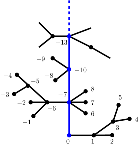
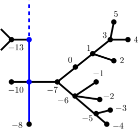
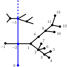
Figure 1: An infinite tree rooted at $0$, seen from $-8$ and relabelled.

We denote by $\mathcal{T}_{c}$ a Bienaymé-Galton Watson tree with offspring distribution $\mu$. The tree $\mathcal{T}_{c}$ is almost surely finite, but conditioned on being large, say having $n$ nodes, it has of the order of $\sqrt{n}$ generation and the set of positions, $\mathcal{T}^{x}_{c}$, typically fills a ball of volume $n^{d/4}$. The cases $d\geq 5$ are called by physicists the upper-critical space dimensions, when considering the BRW. For probabilists, when $d\geq 5$ the critical BRW is transient in the sense that a BRW, conditioned on having size $n$, visits the origin a finite number of times independent of $n$, and the expected number of visits of a site (the so-called Green’s function) is well defined. Dimension four is the critical dimension for BRW, and there the number of visits to the origin grows logarithmically (in the size of the critical tree). We mention here the works of Le Gall and Lin [LGL15, LGL16] in the transient dimensions that obtained laws of large numbers for the volume of the set of visited sites, when conditioning the BRW to have $n$ nodes, as $n$ goes to infinity. The far-reaching idea behind the law of large numbers is introducing an infinite labelled tree invariant under a shift of the labelling as shown in Figure 1, and its corresponding re-rooting of the tree. On such an invariant object, such as $\mathcal{T}_{-}$, ergodic theory, yields laws of large numbers. The genealogy of the invariant tree looks like a comb whose teeth are independent critical trees, with respective volumes being independent heavy tailed variables (since by Kolmogorov’s estimate $\mathbb{P}(|\mathcal{T}_{c}|>t)\asymp\frac{1}{\sqrt{t}}$). This allowed Le Gall and Lin to retrieve information on the critical tree from the infinite invariant ones. Then, building on their beautiful observations, Zhu [Zhu16a] defines, in $d\geq 5$, the branching capacity of a set, and links it to the probability that a critical BRW (indexed by $\mathcal{T}_{c}$) or an infinite BRW (indexed by $\mathcal{T}_{-}$) hits the set, properly normalised. With our notation, Zhu’s key results read as follows.

$$\lim_{\|x\|\to\infty}\frac{\mathbb{P}(\mathcal{T}_{c}^{x}\text{ hits }K)}{g(x)}\,=\,\mathrm{BCap}(K)\,=\,\lim_{\|x\|\to\infty}\frac{\mathbb{P}(\mathcal{T}^{x}_{-}\text{ hits }K)}{G(x)},$$ (1.1)

where $g$ (respectively $G$) is the Green’s function for the critical tree $\mathcal{T}_{c}^{x}$ (resp. for the infinite tree $\mathcal{T}_{-}^{x}$). In other words,

$$g(x)=\mathbb{E}\!\left[\sum_{u\in\mathcal{T}_{c}}{\text{\Large$\mathfrak{1}$}}(S_{u}^{0}=x)\right],\quad\text{and}\quad G(x)=\mathbb{E}\!\left[\sum_{u\in\mathcal{T}_{-}}{\text{\Large$\mathfrak{1}$}}(S_{u}^{0}=x)\right].$$

Note that by criticality of the tree, the function $g$ is the same as the Green’s function for simple random walk.

Moreover, [Zhu16a] gives a dual definition of branching capacity in terms of escape probabilities:

$$\mathrm{BCap}(K)=\sum_{x\in K}\mathbb{P}(\mathcal{T}_{-}^{x}\cap K=\emptyset).$$ (1.2)

In view of these findings, a transient branching random walk seems to resemble a transient random walk. What about a last passage decomposition? Let us recall what it amounts to for a simple random walk, denoted here by $(X_{n})_{n\geq 0}$. When starting at $x$, we denote its law by $\mathbb{P}_{x}$, and for any subset $K\subset\mathbb{Z}^{d}$, we denote by $H_{K}=\inf\{n\geq 0:X_{n}\in K\}$ and $H_{K}^{+}=\inf\{n\geq 1:X_{n}\in K\}$, the first hitting and the first return time to $K$ respectively. Then we have a last passage decomposition

$$\mathbb{P}_{x}(H_{K}<\infty)=\sum_{y\in K}\sum_{n\in\mathbb{N}}\mathbb{P}_{x}\big{(}X_{n}=y,\ \{X_{n+k}:k\geq 1\}\text{ avoids }K\big{)}.$$ (1.3)

We next use the Markov property and invariance by time shift to get, for any $x\in\mathbb{Z}^{d}$

$$\mathbb{P}_{x}(H_{K}<\infty)=\sum_{y\in K}g(x-y)\cdot\mathbb{P}_{y}(H_{K}^{+}=\infty).$$ (1.4)

For a tree this Markov property fails and this is the main source of difficulty in this setting. The fundamental formula (1.4) is at the heart of the potential theory for random walks, and can also be thought of as a relation between the function $x\mapsto\mathbb{P}_{x}(H_{K}<\infty)$, which equals one on $K$ and is harmonic outside $K$, the Green’s function $g$ and the equilibrium measure. Such an exact formula in the context of branching random walks is missing due to the lack of Markov property, and so far it has prevented the development of a satisfactory potential theory for branching random walks, despite the series of works by Zhu [Zhu16a, Zhu16b, Zhu18, Zhu19, Zhu20, Zhu21] that laid its foundations. The main goal of this paper is to establish a relation between the Green’s function and the equilibrium measure similar to (1.4). As a main application we are able to establish an approximate variational characterisation, see Corollary 1.4.

Our second result is obtained independently of the approximate last passage decomposition and provides exponential moment bounds on certain functionals of the BRW for both the infinite tree and the critical one. Using these results, we estimate the probability the BRW spends a large time in each of the balls making up a domain $\Lambda$, in terms of the branching capacity of $\Lambda$, in an analogous form as for the simple random walk.

We then give two other corollaries of our results: (i) Euclidean balls are sets of minimal branching capacity (up to constant), given their volume, and (ii) in each finite set $\Lambda\subset\mathbb{Z}^{d}$, there is a subset whose branching capacity and volume are of order the branching capacity of $\Lambda$, which were instrumental for solving large deviations problems on the range, see below.

Before stating precisely our results, we recall the definitions of equilibrium measure and branching capacity, which were introduced by Zhu in [Zhu16a]. We assume from now on and until the end of the paper that $d\geq 5$.

Definition 1.2.

Let $K$ be a finite subset of $\mathbb{Z}^{d}$. The equilibrium measure of $K$ is the measure defined for $x\in\mathbb{Z}^{d}$, by

$$e_{K}(x)={\text{\Large$\mathfrak{1}$}}(x\in K)\cdot\mathbb{P}(\mathcal{T}_{-}^{x}\cap K=\emptyset).$$

The branching capacity of $K$ is defined to be

$$\mathrm{BCap}(K)=\sum_{x\in K}e_{K}(x).$$

Our first result provides an approximate last passage decomposition.

Theorem 1.3.

There exist positive constants $c$ and $C$, so that for any finite set $K\subseteq\mathbb{Z}^{d}$, we have

$$\|Ge_{K}\|_{\infty}=\max_{x\in\mathbb{Z}^{d}}\,Ge_{K}(x):=\max_{x\in\mathbb{Z}^{d}}\sum_{y\in K}G(x,y)e_{K}(y)\leq C,$$ (1.5)

and if $K$ is nonempty,

$$\min_{x\in K}\,Ge_{K}(x)\geq c.$$ (1.6)

One application of this result is an approximate variational characterisation of the branching capacity, which solves an open question of [Zhu20].

Corollary 1.4.

There exist positive constants $C_{1},C_{2}$, such that for any finite nonempty set $K\subseteq\mathbb{Z}^{d}$,

$$\frac{C_{1}}{\mathrm{BCap}(K)}\leq\inf\Big{\{}\sum_{x,y\in K}G(x-y)\,\nu(x)\nu(y):\nu\textrm{ probability measure on }K\Big{\}}\leq\frac{C_{2}}{\mathrm{BCap}(K)}.$$ (1.7)

We shall give two proofs of this corollary. One, based on the method of [BPP95], which only uses (1.5), but requires a finite third moment on $\mu$, and a second one which needs both (1.5) and (1.6), but only requires a finite second moment on $\mu$.

Our second main result is an exponential moment bound for functionals of the infinite BRW, which can be thought of as an extension of Kac’s moment formula to a non-Markovian setting, see e.g. [S12, Proposition 2.9], and is obtained independently of Theorem 1.3.

Theorem 1.5.

Assume that $\mu$ has a finite exponential moment. There exists $\kappa>0$, such that for any map $\varphi:\mathbb{Z}^{d}\to[0,\infty)$, satisfying $\|G\varphi\|_{\infty}\leq\kappa$, one has

$$\mathbb{E}\!\left[\exp\Big{(}\sum_{u\in\mathcal{T}}\varphi(S_{u})\Big{)}\right]\leq 2.$$

Theorem 1.5 is useful if we can find a potential $\varphi$ with $\|G\varphi\|_{\infty}\leq\kappa$, and Theorem 1.3 provides such a family of functions: we build them from the equilibrium potential $e_{K}$, with appropriate $K$.

Our proof of Theorem 1.5 uses a moment method, which bears similarities with the one in [AHJ21]. However, while [AHJ21] handles any dimension, including the intricate dimension four, it restricts its analysis to the case when $\varphi$ is supported on a single point. Our approach is a priori restricted to dimensions five and higher but we are able to consider any function satisfying $\|G\varphi\|_{\infty}\leq\kappa$, which is ideally suited to study covering of a given domain of space by BRW, and our recursion method is elementary.

When combined together our two main results have a number of interesting consequences. A first immediate application is a large deviations upper bound for the time spent on a collection of balls. For $x\in\mathbb{Z}^{d}$, and $r>0$, write $B(x,r)$ for the Euclidean closed ball of radius $r$ centered at $x$ (intersected with $\mathbb{Z}^{d}$), and for a subset $\mathcal{C}\subset\mathbb{Z}^{d}$, define $B(\mathcal{C},r)=\cup_{x\in\mathcal{C}}B(x,r)$.

For $x,y\in\mathbb{Z}^{d}$, we define

$$\ell_{\mathcal{T}^{x}}(y)=\sum_{u\in\mathcal{T}}{\text{\Large$\mathfrak{1}$}}(S^{x}_{u}=y),$$

and for $A\subseteq\mathbb{Z}^{d}$, we write $\ell_{\mathcal{T}^{x}}(A)=\sum_{y\in A}\ell_{\mathcal{T}^{x}}(y)$.

Corollary 1.6.

Assume that $\mu$ has a finite exponential moment. Then there exists $\kappa>0$, such that for any $t>0$, any $r\geq 1$, and any finite set $\mathcal{C}\subset\mathbb{Z}^{d}$,

$$\mathbb{P}\Big{(}\ell_{\mathcal{T}^{0}}(B(x,r))>t,\text{ for all }x\in\mathcal{C}\Big{)}\leq 2\exp\Big{(}-\kappa\cdot\frac{t}{r^{d}}\cdot\mathrm{BCap}(B(\mathcal{C},r))\Big{)}.$$ (1.8)

Remark 1.7.

Note that since $\mathcal{T}$ contains $\mathcal{T}_{c}$ as subtree, the same result holds as well with $\mathcal{T}_{c}^{0}$ instead of $\mathcal{T}^{0}$ (and this remark applies to Theorem 1.5 as well).

Also, it was proved in [Zhu16a] that the branching capacity of a ball of radius $r$ is of order $r^{d-4}$, thus in the case of one ball we recover the results of [AHJ21, AS22]. We note that the case of dimension four would require a completely different strategy, and is open (except for one ball). The question of obtaining a corresponding lower bound is also interesting, but even in the case of a single random walk, which form the lower bound should take is not clear to us.

Let us mention that in the setting of a simple random walk the argument used here for proving Corollary 1.6 provides an alternative and more direct approach for Theorem 1.2 from [AS23a], see also Remark 4.8.

We present now a result which has proved useful in studying the folding of a random walk in large deviations problems on the range, as in [AS23a], and also played an important role in the context of random interlacements [S21, S23].

Corollary 1.8.

There exists $\alpha>0$, such that for any $r\geq 1$ and any finite $\mathcal{C}\subset\mathbb{Z}^{d}$, there is a subset $U\subseteq\mathcal{C}$, satisfying

$$(i)\quad\mathrm{BCap}(\cup_{x\in U}B(x,r))\geq\alpha\cdot r^{d-4}|U|\quad\text{and}\quad(ii)\quad r^{d-4}|U|\geq\alpha\cdot\mathrm{BCap}(\cup_{x\in\mathcal{C}}B(x,r)).$$ (1.9)

Another application of Theorem 1.5 is the following general upper deviations bound for the time spent in an arbitrary set. Define for $x\in\mathbb{Z}^{d}$, and $\Lambda\subset\mathbb{Z}^{d}$, $G(x,\Lambda)=\sum_{y\in\Lambda}G(x,y)$.

Corollary 1.9.

Assume that $\mu$ has a finite exponential moment. Then there exists $c>0$, such that for any $t>0$ and any finite nonempty set $\Lambda\subset\mathbb{Z}^{d}$, one has

$$\mathbb{P}(\ell_{\mathcal{T}^{0}}(\Lambda)>t)\leq 2\exp\left(-c\cdot\frac{t}{\sup_{x\in\mathbb{Z}^{d}}G(x,\Lambda)}\right).$$

Note that $G(x,\Lambda)\leq C|\Lambda|^{4/d}$, for some universal constant $C$ which does not depend on $\Lambda$ nor on $x\in\mathbb{Z}^{d}$, thus in the above corollary, one could as well replace the denominator in the exponential by $|\Lambda|^{4/d}$. However, the slightly more general form presented here can be useful in some situations when e.g. the set $\Lambda$ has a small local density, as in [AS21, AS23b].

In the standard framework of random walks, Corollaries 1.6, 1.8 and 1.9 were instrumental in studying the moderate deviations of the range in [AS17, AS21, AS23a], and for solving a long-standing conjecture of Khanin, Mazel, Schlossman and Sinai [KMSS94] concerning the large deviations for the intersection of two independent ranges in [AS23b]. We expect that our tools will permit analogous questions to be handled in upper-critical dimensions for BRW.

For completeness and to emphasise the analogy with a single random walk we provide two other variational characterisations.

Corollary 1.10.

There exist positive constants $C_{3},C_{4}$, such that for any finite set $K\subset\mathbb{Z}^{d}$,

$$C_{3}\cdot\mathrm{BCap}(K)\leq\sup\Big{\{}\sum_{x\in K}\varphi(x):\varphi\geq 0\text{ on }K,\,\max_{x\in K}G\varphi(x)\leq 1\Big{\}}\leq C_{4}\cdot\mathrm{BCap}(K),$$ (1.10)

and

$$C_{3}\cdot\mathrm{BCap}(K)\leq\inf\Big{\{}\sum_{x\in K}\varphi(x):\varphi\geq 0\text{ on }K,\,\min_{x\in K}G\varphi(x)\geq 1\Big{\}}\leq C_{4}\cdot\mathrm{BCap}(K).$$ (1.11)

Finally another immediate application of Theorem 1.3 is the following general lower bound for the branching capacity of a set in terms of its volume.

Corollary 1.11.

There exists a positive constant $c>0$, such that for any finite set $K\subset\mathbb{Z}^{d}$,

$$\mathrm{BCap}(K)\geq c|K|^{1-\frac{4}{d}}.$$

Together with the fact already mentioned that the branching capacity of a ball $B(x,r)$ is of order $r^{d-4}$, this shows that as for the usual Newtonian capacity, balls are sets having minimal branching capacity among those with fixed volume (at least up to universal constants).

The non-Markovian nature of the BRW. We mentioned already that this work can be seen as extending some key random walk potential theoretic results to a non-Markovian setting: the infinite invariant tree defined above. We describe the latter informally as being a one-sided infinite random walk, the so-called spine, on each node of which there are two critical trees hanging off, one in the past and the other one in the future. It is only when conditioning on the spine that we can disentangle past and future. However, as we average over both the spine and its dangling trees there is often a subtle tradeoff between what is required from the spine, and what the dangling trees achieve. We use extensively that we are in a regime where the typical behaviour is dominant, and the spine is a simple random walk which typically spends time $L^{2}$ in a region of diameter $L$. If we can place ourselves in a situation where the dangling trees all see the same environment (typically avoid some set far away) then their initial position is innocuous, and we can use uniform bounds on them.

Organisation. The rest of the paper is organised as follows. In Section 2 we provide some preliminary results, such as the shift-invariance of the infinite tree, some basic facts about Green’s functions, and also about the equilibrium measure. We also recall important results of Zhu on hitting probability estimates. In Section 3 we first give a sketch of the proof of (1.5) and in the remaining section we give the full proof as well as provide a first proof of Corollary 1.4, that only uses the upper bound part of Theorem 1.3. In Section 4 we prove Theorem 1.5, together with Corollary 1.6. Then in Section 5 we prove (1.6), which concludes the proof of Theorem 1.3. Finally in Section 6, we give another short proof of Corollary 1.4, and prove the remaining results, Corollaries 1.8, 1.9, 1.10, and 1.11.

2 Preliminaries

2.1 General notation

Given two real functions $f$ and $g$, we write $f\lesssim g$, or sometimes $f=\mathcal{O}(g)$, when there exists a constant $C>0$, such that $f(x)\leq Cg(x)$, for all $x$. We write $f\asymp g$, when both $f\lesssim g$ and $g\lesssim f$. We write $f\sim g$, when $f(x)/g(x)\to 1$, as $x\to\infty$.

Given $A\subset\mathbb{Z}^{d}$, we let $A^{c}:=\mathbb{Z}^{d}\backslash A$, and we define the boundary $\partial A$ of $A$ as the set of elements of $A$ which have at least one neighbor in $A^{c}$.

We let $\|x\|$ denote the Euclidean norm of an element $x\in\mathbb{Z}^{d}$. We write $a\wedge b$ and $a\vee b$ respectively for the minimum and maximum between two real numbers $a$ and $b$. For $r>0$, we write $G(r)=r^{4-d}$.

2.2 Trees and tree-indexed random walks

Let $\widetilde{\mu}$ be the probability measure defined by $\widetilde{\mu}(i)=\sum_{j\geq i+1}\mu(j)$. A tree where only the distribution of the offspring of the root is $\widetilde{\mu}$ and everywhere else it is $\mu$ is called a $\mu$-adjoint tree and we denote it by $\widetilde{\mathcal{T}}_{c}$.

Definition 2.1.

We define the shift transformations $\theta$ and its inverse $\theta^{-1}$ on $\mathcal{T}$ by adding $1$, respectively $-1$, to all labels and then the vertex with label $0$ becomes the new root. Furthermore, these maps extend naturally to transformations on the law of the random walk indexed by $\mathcal{T}$.

Proposition 2.2.

The laws of $\mathcal{T}$ and of the random walk indexed by $\mathcal{T}$ are invariant under the shift transformations $\theta$ and $\theta^{-1}$.

We refer the reader to [Zhu18] or [BW22] for a full proof of this proposition. The fact that the law of the random walk indexed by $\mathcal{T}_{+}$ is invariant under $\theta^{-1}$ was first observed by Le Gall and Lin [LGL15, LGL16], and is reminiscent of the invariance property of sin-trees discovered by Aldous [Ald91].

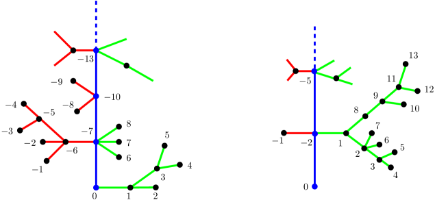
Figure 2: Applying the shift transformation $\theta^{8}$: the blue part is the spine, the green part is the future and the red part is the past.

For a special vertex $u$ of $\mathcal{T}$ (i.e. on the spine of $\mathcal{T}$) we write $k_{\mathrm{p}}(u)$ and $k_{\mathrm{f}}(u)$ for the number of normal offsprings of $u$ in the past and future of $\mathcal{T}$ respectively. By the construction of $\mathcal{T}$ we then see that for all $i,j\in\mathbb{N}$,

$$\mathbb{P}\!\left(k_{\mathrm{p}}(u)=i,k_{\mathrm{f}}(u)=j\right)=\mu(i+j+1),$$

and hence both $k_{\mathrm{p}}(u)$ and $k_{\mathrm{f}}(u)$ are distributed according to $\widetilde{\mu}$. As a consequence, the subtrees of $\mathcal{T}$ emanating from the vertices on the spine, either in the past or in the future, are $\mu$-adjoint trees. A random walk indexed by a $\mu$-adjoint tree is called an adjoint branching random walk.

For $n\geq 0$, we let $\mathcal{T}^{x}(n)$ be the value of the random walk indexed by $\mathcal{T}$ starting from $x$ at the vertex with label $n\in\mathbb{Z}$, and similarly for the other tree-indexed walks. For $a\leq b$ in $\mathbb{Z}$, we write $\mathcal{T}^{x}[a,b]:=\{\mathcal{T}^{x}(n)\}_{n\in[a,b]}$, and similarly for $\mathcal{T}^{x}[a,b)$, $\mathcal{T}^{x}(a,b]$, or for other random trees. We write $(X^{x}(n))_{n\in\mathbb{N}}$ for the random walk indexed by the spine parametrised by its intrinsic labelling (i.e. its natural time parametrisation), when it starts from $x\in\mathbb{Z}^{d}$.

With a slight abuse of notation we shall sometimes denote the tree-indexed random walk (as a process) by $\mathcal{T}^{x}$ (which was formally defined as a random subset of $\mathbb{Z}^{d}$). For integers $0\leq a\leq b\leq\infty$, we also write $\mathcal{F}_{-}^{x}[a,b]$ (respectively $\mathcal{F}_{+}^{x}[a,b]$) for the positions of $\mathcal{T}^{x}$ on the set of vertices lying in the adjoint trees in the past (respectively future) emanating from the points on the spine with time index (in the natural parametrisation of the spine) in $[a,b]$, and similarly with $[a,b)$. See Figure 2 for an illustration of these definitions.

2.3 Basic facts on Green’s functions and branching capacity

We denote by $g$ the Green’s function of a simple random walk $(X_{n})_{n\geq 0}$, in other words:

$$g(x,y)=\mathbb{E}_{x}\Big{[}\sum_{n=0}^{\infty}{\text{\Large$\mathfrak{1}$}}(X_{n}=y)\Big{]}=g(0,y-x),$$

where $\mathbb{E}_{x}$ denotes the expectation for a walk starting from $x$. Recall that (see e.g. [LL10]),

$$g(x,y)\asymp\frac{1}{1+\|x-y\|^{d-2}}.$$ (2.1)

In fact by linearity of expectation and criticality of $\mu$, one also has

$$g(x,y)=\mathbb{E}\Big{[}\sum_{u\in\mathcal{T}_{c}}{\text{\Large$\mathfrak{1}$}}(S_{u}^{x}=y)\Big{]}.$$

Similarly we define

$$G(x,y)=G(y-x)=\mathbb{E}\Big{[}\sum_{u\in\mathcal{T}_{-}}{\text{\Large$\mathfrak{1}$}}(S_{u}^{x}=y)\Big{]}.$$

Since the mean number of normal offspring of a vertex on the left of the spine of $\mathcal{T}$ has mean $\sigma^{2}/2$, we deduce that for any $x,y\in\mathbb{Z}^{d}$,

$$G(x,y) =\sum_{z\in\mathbb{Z}^{d}}\Big{(}g(x,z)-{\text{\Large$\mathfrak{1}$}}(z=x)\Big{)}\cdot\Big{(}{\text{\Large$\mathfrak{1}$}}(z=y)+\frac{\sigma^{2}}{2}(g(z,y)-{\text{\Large$\mathfrak{1}$}}(z=y))\Big{)}$$

$$=\frac{\sigma^{2}}{2}\sum_{z\in\mathbb{Z}^{d}}g(x,z)g(z,y)+\mathcal{O}(g(x,y)).$$ (2.2)

Using (2.1), this yields

$$G(x,y)\asymp\frac{1}{1+\|x-y\|^{d-4}}.$$ (2.3)

We now state some important facts related to the equilibrium measure and the branching capacity. The next proposition is a simple last passage decomposition formula which will be used widely in the paper.

Proposition 2.3.

Let $K^{\prime}\subseteq K$ and $B$ be finite subsets of $\mathbb{Z}^{d}$ such that $B$ contains $K^{\prime}$ and points at distance $1$ from $K^{\prime}$. Then

$$\sum_{y\in K^{\prime}}e_{K}(y)=\sum_{w\in\partial B}\mathbb{P}\!\left(\mathcal{T}_{-}^{w}\cap(K\cup B)=\emptyset,\mathcal{T}^{w}_{+}\text{ first hits }K\text{ in }K^{\prime}\right).$$

Proof.

Let $L$ be the last time that the past of the tree-indexed random walk is in $B$. For all $y\in K^{\prime}$ we can now write

$$e_{K}(y)=\mathbb{P}\!\left(\mathcal{T}^{y}_{-}\cap K=\emptyset\right)=\sum_{w\in\partial B}\sum_{n\geq 1}\mathbb{P}\!\left(\mathcal{T}_{-}^{y}\cap K=\emptyset,\mathcal{T}^{y}(-n)=w,L=n\right),$$

since $L$ is finite almost surely. Using the invariance of the tree $\mathcal{T}^{y}$ under the shift $\theta^{n}$ by Proposition 2.2 we get

$$\mathbb{P}\!\left(\mathcal{T}_{-}^{y}\cap K=\emptyset,\mathcal{T}^{y}(-n)=w,L=n\right)=\mathbb{P}\!\left(\mathcal{T}^{w}(n)=y,\mathcal{T}_{-}^{w}\cap(K\cup B)=\emptyset,\mathcal{T}^{w}[0,n)\cap K=\emptyset\right).$$

Taking now the sum over all $y\in K^{\prime}$ and all $n\geq 1$ completes the proof. ∎

For a finite subset $K\subset\mathbb{Z}^{d}$, and $A\subseteq\mathbb{Z}^{d}$, we write $e_{K}(A)=\sum_{x\in A}e_{K}(x)$.

Lemma 2.4.

For any finite set $K\subseteq\mathbb{Z}^{d}$ containing two disjoint sets $U$ and $V$, we have

$$e_{K}(U\cup V)\geq e_{K\backslash V}(U).$$

Remark 2.5.

An immediate consequence of this lemma is that the branching capacity is monotone for inclusion, a fact already proved by [Zhu16a]. Indeed, applying the lemma with $V=K\backslash U$, gives that if $U\subseteq K$, then $\mathrm{BCap}(U)\leq\mathrm{BCap}(K)$.

Proof of Lemma 2.4.

Let $R>0$, be such that $K\subset B(0,R-1)$. Applying Proposition 2.3 we get

$$e_{K}(U\cup V)=\sum_{w\in\partial B(0,R)}\mathbb{P}\big{(}\mathcal{T}_{-}^{w}\cap B(0,R)=\emptyset,\mathcal{T}^{w}_{+}\text{ first hits $K$ in }U\cup V\big{)}.$$

Observing that $\{\mathcal{T}_{+}^{w}\text{ first hits }K\backslash V\text{ in }U\}\subseteq\{\mathcal{T}_{+}^{w}\text{ first hits }K\ \text{in }U\cup V\}$, we then obtain

$$e_{K}(U\cup V)\geq\sum_{w\in\partial B(0,R)}\mathbb{P}\big{(}\mathcal{T}_{-}^{w}\cap B(0,R)=\emptyset,\mathcal{T}_{+}^{w}\text{ first hits }K\backslash V\text{ in }U\big{)}=e_{K\setminus V}(U),$$

applying Proposition 2.3 again for the last equality. ∎

The next result provides the exact order of magnitude of the branching capacity of balls.

Proposition 2.6 ([Zhu16a]).

There exist positive constants $c_{1},c_{2}$, such that for all $r\geq 1$,

$$c_{1}\cdot r^{d-4}\leq\mathrm{BCap}(B(0,r))\leq c_{2}\cdot r^{d-4}.$$

We shall often use later, without further reference that for a set $K\subseteq B(0,R)$, one has $\mathrm{BCap}(K)\lesssim R^{d-4}$, which follows from a combination of the last two results.

2.4 Hitting probability for a branching random walk

Definition 2.7.

Suppose that $S$ is a random walk indexed by a spatial rooted tree $T$. On the event that $S$ hits a set $A$ we define the first entry vertex to $A$ as the smallest vertex $u\in T$ in the lexicographical order for which $S_{u}\in A$. If the unique path from the root of $\mathcal{T}$ to the first entry vertex of $A$ is given by $(v_{0},v_{1},\ldots,v_{k})$ for some $k\in\mathbb{N}$, then we set $\Gamma(S)=(S_{v_{0}},\ldots,S_{v_{k}})$. We say that $S$ hits $A$ via $\gamma$, if $\Gamma(S)=\gamma$. We also say that $S$ first hits the set $A$ in $a\in A$ if at the first entry vertex to $A$ the walk $S$ is at $a$.

Recall that $\widetilde{\mathcal{T}^{x}_{c}}$ denotes the range of an adjoint branching random walk starting from $x$. For a set $A\subseteq\mathbb{Z}^{d}$, we write

$$b_{A}(x)=\mathbb{P}\big{(}\widetilde{\mathcal{T}}_{c}^{x}\cap A=\emptyset\big{)}.$$

For a path $\gamma:\{0,\dots,N\}\to\mathbb{Z}^{d}$ we write $|\gamma|=N$, i.e. $|\gamma|$ is the length of $\gamma$ without its first point. We write $s(\gamma)$ for the probability that a simple random walk started from $\gamma(0)$ follows this path for its first $|\gamma|$ steps. We say that $\gamma$ starts from $x$ if $\gamma(0)=x$, and that it goes from $x$ to a set $A$ and write $\gamma:x\to A$, if in addition $\gamma(N)\in A$ and $\gamma(\ell)\notin A$ for all $\ell<N$. Given $x,y\in\mathbb{Z}^{d}$, we write $\gamma:x\to y$ if $\gamma(0)=x$ and $\gamma(N)=y$.

Proposition 2.8 ([Zhu16a, Proposition 5.1]).

Let $A\subset\mathbb{Z}^{d}$ and $x\in A^{c}$. Then for any $\gamma:x\to A$ we have

$$\mathbb{P}(\mathcal{T}^{x}_{c}\text{ hits $A$ via $\gamma$})=s(\gamma)\prod_{\ell=0}^{|\gamma|-1}b_{A}(\gamma(\ell)).$$

We now recall some hitting probability estimates obtained by Zhu. Given $x\in\mathbb{Z}^{d}$ and $K\subset\mathbb{Z}^{d}$, we let $d(x,K)=\inf\{\|x-y\|:y\in K\}$, and $\text{diam}(K)=\sup\{\|x-y\|:x,y\in K\}$.

Theorem 2.9 ([Zhu16a, Zhu16b]).

Let $\varepsilon>0$ be fixed. There exist positive constants $c_{1},c_{2}$, such that for any finite nonempty $K\subset\mathbb{Z}^{d}$ and any $x\in\mathbb{Z}^{d}$, with $d(x,K)\geq\varepsilon\cdot\textrm{diam}(K)$, one has

$$c_{1}\frac{\mathrm{BCap}(K)}{d(x,K)^{d-4}}\leq\mathbb{P}\big{(}\mathcal{T}_{-}^{x}\cap K\neq\emptyset\big{)}\leq c_{2}\frac{\mathrm{BCap}(K)}{d(x,K)^{d-4}},$$ (2.4)

and

$$c_{1}\frac{\mathrm{BCap}(K)}{d(x,K)^{d-2}}\leq\mathbb{P}\big{(}\mathcal{T}_{c}^{x}\cap K\neq\emptyset\big{)}\leq c_{2}\frac{\mathrm{BCap}(K)}{d(x,K)^{d-2}}.$$ (2.5)

Remark 2.10.

We note that the same estimate as (2.5) holds as well for $\widetilde{\mathcal{T}}_{c}^{x}$.

3 Upper bound on $\|Ge_{K}\|_{\infty}$

In this section we give the proof of the first part of Theorem 1.3, namely (1.5). Using (1.5) we then give a proof of Corollary 1.4 assuming a finite third moment on $\mu$. We start with a sketch of the proof in Section 3.1. Then after recalling some standard estimates for a simple random walk in Section 3.2, we state and prove some results on hitting times for branching random walks in Section 3.3. The proofs of (1.5) and Corollary 1.4 are deferred to Sections 3.4 and 3.5 respectively.

3.1 Sketch of proof of (1.5)

First, since we seek an upper bound of $Ge_{K}(x)$, which is uniform in $K$ and $x$, one can always assume that $x$ is at the origin. Now by decomposing $K$ into slices $K=\cup_{i}K_{i}$, where $K_{i}=K\cap\{2^{i}\leq\|x\|\leq 2^{i+1}\}$, we find that

$$Ge_{K}(0)\asymp\sum_{i}G(2^{i})e_{K}(K_{i}),$$

with $e_{K}(K_{i})=\sum_{y\in K_{i}}e_{K}(y)$. Thus one needs to estimate $e_{K}(K_{i})$ now. For each $y\in K_{i}$, we decompose the event $\{\mathcal{T}^{y}_{-}\cap K=\emptyset\}$ according to the last point on $\partial B(0,2^{i+2})$ visited by the spine, and using shift invariance of the tree we arrive at

$$e_{K}(K_{i})\leq\sum_{w\in\partial B(0,2^{i+2})}\mathbb{P}\big{(}\mathcal{T}^{w}_{+}\cap K_{i}\neq\emptyset,\mathcal{T}_{-}^{w}\cap(B_{i+2}\cup K)=\emptyset\big{)},$$

see (3.6) below. If the past and future trees were independent, we could separate both events in the probability on the right-hand side. Now for any $w\in\partial B(0,2^{i+2})$, by (2.4) (which holds as well for $\mathcal{T}_{+}^{w}$), one has

$$\mathbb{P}\big{(}\mathcal{T}^{w}_{+}\cap K_{i}\neq\emptyset)\asymp G(2^{i})\cdot\textrm{BCap}(K_{i}),$$

while by Proposition 2.6,

$$\sum_{w\in\partial B(0,2^{i+2})}\mathbb{P}\big{(}\mathcal{T}^{w}_{-}\cap B_{i+2}=\emptyset\big{)}=\textrm{BCap}\big{(}B(0,2^{i+2})\big{)}\lesssim\frac{1}{G(2^{i})}.$$

Moreover, at a heuristic level the events $\{\mathcal{T}^{w}_{-}\cap K_{j}=\emptyset\}$, for $j\geq i+3$, can be considered as being almost independent, and also independent of the event $\{\mathcal{T}^{w}_{-}\cap B_{i+2}=\emptyset\}$, since they depend on different pieces of $\mathcal{T}_{-}^{w}$ involving different scales. Thus we may infer that for some constant $c>0$,

$$\mathbb{P}\big{(}\mathcal{T}_{-}^{w}\cap(B_{i+2}\cup K)=\emptyset\big{)}\lesssim\frac{1}{G(2^{i})}\cdot\prod_{j\geq i+3}\Big{(}1-c\cdot G(2^{j})\textrm{BCap}(K_{j})\Big{)}.$$

Therefore, under these rough independence assumptions, we arrive at

$$G(2^{i})e_{K}(K_{i})\lesssim G(2^{i})\textrm{BCap}(K_{i})\cdot\exp\Big{(}-c\sum_{i+3\leq j\leq I}G(2^{j})\textrm{BCap}(K_{j})\Big{)},$$ (3.1)

where $I$ is the maximal index $i$ such that $K_{i}$ is nonempty, and we conclude by observing that for any sequence $(\varepsilon_{i})_{i\geq 0}$, bounded by one,

$$\sup_{I\geq 1}\,\sum_{i\leq I}\varepsilon_{i}\cdot\exp\Big{(}-c\sum_{j\geq i+3}\varepsilon_{j}\Big{)},$$

is bounded by a constant that does not depend on the sequence $(\varepsilon_{i})_{i\geq 1}$. Now of course, while we will prove that (3.1) is indeed correct, the whole technical matter of the proof is to deal with the fact that the events above are not really independent. In particular it is only once we condition on the positions of the walk on the spine that the past and future can be decorrelated. However, to make the arguments work fine, one also needs to ensure that one can place ourselves on the typical event, when the spine spends a time of order $2^{2j}$ in each of the sets $\{2^{j}\leq\|x\|\leq 2^{j+1}\}$, which leads to some technical difficulties.

3.2 Simple random walk estimates

We collect here a number of preliminary estimates concerning the simple random walk on $\mathbb{Z}^{d}$, that will be used for the proof of (1.5). We write $\mathbb{P}_{x}$ for the law of a simple random walk started from $x\in\mathbb{Z}^{d}$ and $\mathbb{E}_{x}$ for the corresponding expectation. We let $X$ be a simple random walk in $\mathbb{Z}^{d}$. For $r>0$, we let $\tau_{r}$ be the first hitting time of $\partial B(0,r)$ and $\tau_{r}^{+}$ the first return time to $B(0,r)$, i.e.

$$\tau_{r}=\inf\{t\geq 0:X_{t}\in\partial B(0,r)\}\quad\text{ and }\quad\tau_{r}^{+}=\inf\{t\geq 1:X_{t}\in\partial B(0,r)\}.$$

Lemma 3.1.

Let $\delta>0$. There exists a positive constant $c=c(\delta)$ such that if $R>0$, then for all $u\in\partial B(0,R)$ we have

$$\mathbb{E}_{u}\!\left[\tau_{R(1+\delta)}\cdot{\text{\Large$\mathfrak{1}$}}(\tau_{R(1+\delta)}<\tau_{R}^{+})\right]\leq cR.$$

Proof.

Let $\tau=\tau_{R(1+\delta)}\wedge\tau_{R}$. Applying the optional stopping theorem to the martingale $(\left\|X_{n}\right\|^{2}-n)_{n\geq 0}$ we obtain that there exists a positive constant $c=c(\delta)$ such that

$$\mathbb{E}_{u}\!\left[\tau_{R(1+\delta)}\cdot{\text{\Large$\mathfrak{1}$}}(\tau_{R(1+\delta)}<\tau_{R}^{+})\right]\leq 1+\sup_{\begin{subarray}{c}v\notin B(0,R)\\ v\sim u\end{subarray}}\mathbb{E}_{v}\!\left[\tau\right]\leq cR$$

and this concludes the proof. ∎

Lemma 3.2.

There exists $c>0$ such that the following holds. Let $R>0$, $u\in\partial B(0,R)$ and $v\in\partial B(0,2R)$. Then

$$\mathbb{P}_{v}\!\left(X_{\tau_{R}}=u,\tau_{R}<cR^{2}\right)\leq\frac{1}{2}\cdot\mathbb{P}_{v}\!\left(X_{\tau_{R}}=u\right).$$

Proof.

Let $\tau=\inf\{t\geq 0:X_{t}\in\partial B(0,3R/2)\}$ be the first hitting time of $\partial B(0,3R/2)$. Let $c$ be a positive constant to be determined later. By the strong Markov property applied to $\tau$ we have

$$\mathbb{P}_{v}\!\left(X_{\tau_{R}}=u,\tau_{R}<cR^{2}\right) =\sum_{w\in\partial B(0,3R/2)}\sum_{n\leq\lfloor cR^{2}\rfloor}\sum_{s<n}\mathbb{P}_{v}\!\left(X_{s}=w,\tau=s\right)\mathbb{P}_{w}\!\left(X_{\tau_{R}}=u,\tau_{R}=n-s\right)$$

$$\leq\sum_{w\in\partial B(0,3R/2)}\sum_{s<\lfloor cR^{2}\rfloor}\mathbb{P}_{v}\!\left(X_{s}=w,\tau=s\right)\mathbb{P}_{w}\!\left(X_{\tau_{R}}=u\right).$$

By a proof similar to [LL10, Lemma 6.3.7], we get that there exist universal constants $c_{1},c_{2}$ so that for all $w\in\partial B(0,3R/2)$ we have

$$\mathbb{P}_{w}\!\left(X_{\tau_{R}}=u\right)\leq\frac{c_{2}}{R^{d-1}}\quad\text{ and }\quad\mathbb{P}_{v}\!\left(X_{\tau_{R}}=u\right)\geq\frac{c_{1}}{R^{d-1}}.$$ (3.2)

Therefore, plugging this above gives

$$\mathbb{P}_{v}\!\left(X_{\tau_{R}}=u,\tau_{R}<cR^{2}\right)\leq\frac{c_{2}}{R^{d-1}}\cdot\mathbb{P}_{v}\!\left(\tau<\lfloor cR^{2}\rfloor\right).$$

On the event $\{\tau<\lfloor cR^{2}\rfloor\}$, the walk must travel distance $R/2$ in time less than $\lfloor cR^{2}\rfloor$, and hence this has probability less than $\exp(-c_{3}/c)$, where $c_{3}$ is a positive constant. Plugging this above gives

$$\mathbb{P}_{v}\!\left(X_{\tau_{R}}=u,\tau_{R}<cR^{2}\right)\leq\frac{c_{2}}{R^{d-1}}\cdot\exp(-c_{3}/c).$$

Taking now $c$ sufficiently small so that $c_{2}\cdot\exp(-c_{3}/c)\leq c_{1}/2$ and using (3.2) we conclude

$$\mathbb{P}_{v}\!\left(X_{\tau_{R}}=u,\tau_{R}<cR^{2}\right)\leq\frac{1}{2}\cdot\frac{c_{1}}{R^{d-1}}\leq\frac{1}{2}\cdot\mathbb{P}_{v}\!\left(X_{\tau_{R}}=u\right),$$

and this finishes the proof. ∎

Lemma 3.3.

There exists a positive constant $c$ so that the following holds. Let $R>0$, $u\in\partial B(0,R)$ and $v\in\partial B(0,2R)$. Then we have

$$\sum_{n\geq 0}n\cdot\mathbb{P}_{u}\!\left(X_{n}=v,\tau_{R}^{+}>n\right)\leq c\cdot R^{2}\cdot\sum_{n\geq 0}\mathbb{P}_{u}\!\left(X_{n}=v,\tau_{R}^{+}>n\right).$$

Proof.

First of all using a reversal argument we see that

$$\sum_{n\geq 0}\mathbb{P}_{u}\!\left(X_{n}=v,\tau_{R}^{+}>n\right)=\mathbb{P}_{v}\!\left(X_{\tau_{R}}=u\right).$$

Since $\mathbb{P}_{v}\!\left(X_{\tau_{R}}=u\right)\asymp R^{1-d}$ (see [LL10, Lemma 6.3.7]), to prove the claim it suffices to show that there exists a positive constant $c$ so that

$$\sum_{n}n\cdot\mathbb{P}_{u}\!\left(X_{n}=v,\tau_{R}^{+}>n\right)\leq\frac{c}{R^{d-3}}.$$ (3.3)

Let $\tau$ be the first hitting time of $\partial B(0,3R/2)$. Then by the strong Markov property applied to $\tau$ we have

$$\sum_{n\geq 0} n\cdot\mathbb{P}_{u}\!\left(X_{n}=v,\tau_{R}^{+}>n\right)$$

$$=\sum_{n\geq 0}\sum_{w\in\partial B(0,3R/2)}\sum_{s<n}n\cdot\mathbb{P}_{u}\!\left(\tau=s,X_{s}=w,\tau<\tau_{R}^{+}\right)\mathbb{P}_{w}\!\left(X_{n-s}=v,\tau_{R}>n-s\right)$$

$$=\sum_{w\in\partial B(0,3R/2)}\sum_{s\geq 0}\mathbb{P}_{u}\!\left(\tau=s,X_{s}=w,\tau<\tau_{R}^{+}\right)\left(\sum_{n>s}n\cdot\mathbb{P}_{w}\!\left(X_{n-s}=v,\tau_{R}>n-s\right)\right)$$

$$\leq\sum_{w\in\partial B(0,3R/2)}\sum_{s\geq 0}\mathbb{P}_{u}\!\left(\tau=s,X_{s}=w,\tau<\tau_{R}^{+}\right)\left(\sum_{n>s}n\cdot\mathbb{P}_{w}\!\left(X_{n-s}=v\right)\right).$$

Using the local central limit theorem we now obtain

$$\sum_{n>s}n\cdot\mathbb{P}_{w}\!\left(X_{n-s}=v\right)=\sum_{n=1}^{\infty}n\cdot\mathbb{P}_{w}\!\left(X_{n}=v\right)+s\cdot\sum_{n=1}^{\infty}\mathbb{P}_{w}\!\left(X_{n}=v\right)\asymp\frac{1}{R^{d-4}}+\frac{s}{R^{d-2}}.$$

Plugging this above we deduce

$$\sum_{n\geq 0}n\cdot\mathbb{P}_{u}\!\left(X_{n}=v,\tau_{R}^{+}>n\right) \lesssim\sum_{w\in\partial B(0,3R/2)}\sum_{s\geq 0}\mathbb{P}_{u}\!\left(\tau=s,X_{s}=w,\tau<\tau_{R}^{+}\right)\cdot\left(\frac{1}{R^{d-4}}+\frac{s}{R^{d-2}}\right)$$

$$=\frac{1}{R^{d-4}}\cdot\mathbb{P}_{u}\!\left(\tau<\tau_{R}^{+}\right)+\frac{1}{R^{d-2}}\cdot\mathbb{E}_{u}\!\left[\tau\cdot{\text{\Large$\mathfrak{1}$}}(\tau<\tau_{R}^{+})\right]\lesssim\frac{1}{R^{d-3}},$$

where we used that Lemma 3.1 for the last inequality. This now concludes the proof. ∎

3.3 Hitting times for branching random walks

For a path $\gamma:\{0,\dots,N\}\to\mathbb{Z}^{d}$, and $A\subseteq\mathbb{Z}^{d}$, we write $\gamma\subseteq A$, if $\gamma(\ell)\in A$, for all $\ell\geq 1$ (note that we allow the starting point of the path to be in $A^{c}$). Recall the notation introduced at the beginning of Section 2.4.

Lemma 3.4.

There exists a positive constant $c$ so that for any $R\geq 1$ any $K\subseteq B(0,R/2)$, any $u\in\partial B(0,R)$ and $v\in\partial B(0,2R)$, one has

$$\sum_{\begin{subarray}{c}\gamma:u\to v\\ \gamma\subseteq B(0,R)^{c}\end{subarray}}s(\gamma)\prod_{\ell=0}^{|\gamma|}b_{K}(\gamma(\ell))\leq\exp\left(-c\frac{\mathrm{BCap}(K)}{R^{d-4}}\right)\cdot\sum_{\begin{subarray}{c}\gamma:u\to v\\ \gamma\subseteq B(0,R)^{c}\end{subarray}}s(\gamma).$$

Proof.

Since $\gamma\subseteq B(0,R)^{c}$ and $K\subseteq B(0,R/2)$, using (2.5) and Remark 2.10 we get that for a positive constant $c$ and for all $\ell\geq 0$

$$b_{K}(\gamma(\ell))\leq 1-c\frac{\mathrm{BCap}(K)}{R^{d-2}}.$$

So taking the product over all $\ell$ we get for a positive constant $c^{\prime}$

$$\prod_{\ell=0}^{|\gamma|}b_{K}(\gamma(\ell))\leq\exp\left(-c^{\prime}|\gamma|\frac{\mathrm{BCap}(K)}{R^{d-2}}\right).$$

Thus we deduce

$$\sum_{\begin{subarray}{c}\gamma:u\to v\\ \gamma\subseteq B(0,R)^{c}\end{subarray}}s(\gamma)\prod_{\ell=0}^{|\gamma|}b_{K}(\gamma(\ell))\leq\sum_{\begin{subarray}{c}\gamma:u\to v\\ \gamma\subseteq B(0,R)^{c}\end{subarray}}s(\gamma)\exp\left(-c^{\prime}|\gamma|\frac{\mathrm{BCap}(K)}{R^{d-2}}\right).$$

Let $c_{1}$ be a positive constant to be determined later. We now show that the last sum above is upper bounded by the sum where we restrict $\gamma$ to have length at least $c_{1}R^{2}$. First we write

$$\sum_{\begin{subarray}{c}\gamma:u\to v\\ \gamma\subseteq B(0,R)^{c}\end{subarray}}s(\gamma)\exp\left(-c^{\prime}|\gamma|\frac{\mathrm{BCap}(K)}{R^{d-2}}\right) \leq\sum_{\begin{subarray}{c}\gamma:u\to v\\ \gamma\subseteq B(0,R)^{c}\\ |\gamma|\leq c_{1}R^{2}\end{subarray}}s(\gamma)+\sum_{\begin{subarray}{c}\gamma:u\to v\\ \gamma\subseteq B(0,R)^{c}\\ |\gamma|>c_{1}R^{2}\end{subarray}}s(\gamma)\exp\left(-c^{\prime}c_{1}\frac{\mathrm{BCap}(K)}{R^{d-4}}\right).$$

Since $\mathrm{BCap}(K)\leq CR^{d-4}$ for a positive constant $C$ we can take $c_{1}$ sufficiently small so that

$$\exp\left(-c^{\prime}c_{1}\frac{\mathrm{BCap}(K)}{R^{d-4}}\right)\leq 1-\frac{c^{\prime}c_{1}}{2}\cdot\frac{\mathrm{BCap}(K)}{R^{d-4}},$$

and hence plugging this above we obtain

$$\sum_{\begin{subarray}{c}\gamma:u\to v\\ \gamma\subseteq B(0,R)^{c}\end{subarray}}s(\gamma)\exp\left(-c^{\prime}|\gamma|\frac{\mathrm{BCap}(K)}{R^{d-2}}\right)$$

$$\leq\left(1-\frac{c^{\prime}c_{1}\mathrm{BCap}(K)}{2R^{d-4}}\right)\cdot\sum_{\begin{subarray}{c}\gamma:u\to v\\ \gamma\subseteq B(0,R)^{c}\end{subarray}}s(\gamma)+\frac{c^{\prime}c_{1}\mathrm{BCap}(K)}{2R^{d-4}}\cdot\sum_{\begin{subarray}{c}\gamma:u\to v\\ \gamma\subseteq B(0,R)^{c}\\ |\gamma|\leq c_{1}R^{2}\end{subarray}}s(\gamma).$$

Taking $c_{1}$ even smaller, applying a time reversal and using Lemma 3.2 we upper bound the quantity above by

$$\left(1-\frac{c^{\prime}c_{1}\mathrm{BCap}(K)}{4R^{d-4}}\right)\cdot\sum_{\begin{subarray}{c}\gamma:u\to v\\ \gamma\subseteq B(0,R)^{c}\end{subarray}}s(\gamma)\leq\exp\left(-c^{\prime}c_{1}\frac{\mathrm{BCap}(K)}{4R^{d-4}}\right)\cdot\sum_{\begin{subarray}{c}\gamma:u\to v\\ \gamma\subseteq B(0,R)^{c}\end{subarray}}s(\gamma),$$

and this concludes the proof. ∎

Lemma 3.5.

For each $R\geq 1$ let $\tau_{R}^{u}$ be the generation of the first hitting vertex of $B(0,R)$ by $\mathcal{T}^{u}_{c}$. There exists $C>0$, such that, for any $R\geq 1$, and any $u\in\partial B(0,2R)$, we have

$$\mathbb{E}\!\left[\tau_{R}^{u}\cdot{\text{\Large$\mathfrak{1}$}}(\tau_{R}^{u}<\infty)\right]\leq C.$$

Proof.

We have

$$\mathbb{E}\!\left[\tau_{R}^{u}\cdot{\text{\Large$\mathfrak{1}$}}(\tau_{R}^{u}<\infty)\right]\leq 2R^{2}\cdot\mathbb{P}\!\left(\tau_{R}^{u}<\infty\right)+R^{2}\cdot\sum_{k\geq 2}\mathbb{P}\!\left(\tau_{R}^{u}\geq kR^{2},\tau_{R}^{u}<\infty\right).$$ (3.4)

Using Theorem 2.9 we get

$$\mathbb{P}\!\left(\tau_{R}^{u}<\infty\right)\lesssim\frac{1}{R^{2}},$$

and hence it only remains to bound the sum appearing on the right hand side of (3.4). We now notice that on the event $\{\tau_{R}^{u}>kR^{2},\tau_{R}^{u}<\infty\}$, there must exist a node on the tree in generation $(k-1)R^{2}$, whose position is not in $B(0,R)$, but which has at least one descendant at distance at least $R^{2}$ from it, whose position is in $B(0,R)$. Writing $Z_{m}$ for the number of vertices in generation $m$ and $\mathcal{S}_{\ell}=B(0,R_{\ell+1})\setminus B(0,R_{\ell})$ with $R_{\ell}=2^{\ell}R$, for $\ell\in\mathbb{N}$, we get

$$\mathbb{P}\!\left(\tau_{R}^{u}\geq kR^{2},\tau_{R}^{u}<\infty\right)\leq \mathbb{E}\!\left[Z_{(k-1)R^{2}}\right]$$

$$\times\sum_{m=0}^{\infty}\mathbb{P}_{u}\!\left(X_{(k-1)R^{2}}\in\mathcal{S}_{m}\right)\max_{x\in\mathcal{S}_{m}}\mathbb{P}\!\left(\mathcal{T}_{c}^{x}\text{ hits }B(0,R)\text{ after $R^{2}$ generations}\right),$$

where $X$ is a simple random walk. For $m=0$ we bound the second probability appearing above by the probability that the tree survives for $R^{2}$ generations, which is of order $1/R^{2}$, by Kolmogorov’s estimate again. For $m\geq 1$ we bound the second probability by $R^{d-4}/R_{m}^{d-2}$ using (2.5) and Proposition 2.6. We also have for a constant $c>0$, by the local central limit theorem, for all $k\geq 2$

$$\mathbb{P}_{u}\!\left(X_{(k-1)R^{2}}\in\mathcal{S}_{m}\right)\lesssim\frac{R_{m}^{d}}{k^{d/2}R^{d}}\wedge\exp\left(-c\frac{R_{m}^{2}}{kR^{2}}\right).$$

Putting everything together we get

$$\sum_{m=1}^{\infty} \mathbb{P}_{u}\!\left(X_{(k-1)R^{2}}\in\mathcal{S}_{m}\right)\max_{x\in\mathcal{S}_{m}}\mathbb{P}\!\left(\mathcal{T}^{x}_{c}\text{ hits }B(0,R)\text{ after $R^{2}$ generations}\right)$$

$$\lesssim\frac{1}{k^{d/2}}\cdot\frac{1}{R^{2}}+\sum_{m\geq 2:R_{m}^{2}\leq kR^{2}}\frac{R_{m}^{d}}{k^{d/2}R^{d}}\cdot\frac{R^{d-4}}{R_{m}^{d-2}}+\sum_{m:R_{m}^{2}>kR^{2}}\exp\left(-c\frac{R_{m}^{2}}{kR^{2}}\right)\cdot\frac{R^{d-4}}{R_{m}^{d-2}}\asymp\frac{1}{R^{2}}\cdot\frac{1}{k^{d/2-1}}.$$

Plugging this back into the sum in (3.4) and using that $\mathbb{E}[Z_{(k-1)R^{2}}]=1$ by criticality of $\mu$, concludes the proof. ∎

3.4 Proof of (1.5)

We prove here the first part of Theorem 1.3. We let $R_{0}=0$ and $R_{i}=2^{i}$ for $i\geq 1$, as well as

$$B_{i}=B(x,R_{i}),\quad\mathcal{S}_{i}=\{y:R_{i}\leq\left\|y-x\right\|\leq R_{i+1}\}\quad\text{ and }\quad K_{i}=K\cap\mathcal{S}_{i}.$$

Let $I$ be the maximal index $i$ such that $K\cap\mathcal{S}_{i}\neq\emptyset$. Then we have

$$\sum_{y\in K}G(x,y)e_{K}(y)\asymp\sum_{i=0}^{I}G(R_{i})\sum_{y\in K_{i}}e_{K}(y).$$ (3.5)

Fix some $0\leq i\leq I$. Then applying Proposition 2.3 with $K^{\prime}=K_{i}$ and $B=B_{i+2}$ we obtain

$$\sum_{y\in K_{i}}e_{K}(y)\leq\sum_{w\in\partial B_{i+2}}\mathbb{P}\!\left(\mathcal{T}_{-}^{w}\cap(B_{i+2}\cup K)=\emptyset,\mathcal{T}_{+}^{w}\cap K_{i}\neq\emptyset\right).$$ (3.6)

We now use the natural parametrisation of the spine and let $X^{w}$ be the simple random walk that the spine performs starting from $w$. Recall that we also write $\mathcal{F}_{-}^{w}[a,b]$ (respectively $\mathcal{F}_{+}^{w}[a,b]$) for the positions of the walk indexed by $\mathcal{T}$ starting from $w$ at vertices lying in the forest consisting of the adjoint trees in the past (respectively future) emanating from the points on the spine with time index (in the natural parametrisation of the spine) in $[a,b]$.

Fix some $w\in\partial B_{i+2}$, and for each $j\geq i+2$ we let $\sigma_{j}$ be the last time that $X^{w}$ is on $\partial B_{j}$, i.e.

$$\sigma_{j}=\sup\{n\geq 0:X^{w}(n)\in\partial B_{j}\}.$$

Note in particular that $\sigma_{i+2}=0$ on the event $\{\mathcal{T}^{w}_{-}\cap B_{i+2}=\emptyset\}$.

Figure 3: The re-rooted tree at $w$ whose spine (in blue) has to avoid $B_{i+2}$ and the past trees (in red) have to avoid $K_{j}$ in the shell $\mathcal{S}_{j}$, whereas the future trees (in green) have to hit $K_{i}$.

For $i,j\in\mathbb{N}$ with $j\geq i+2$ we define

$$A_{i,j}=\{\mathcal{F}_{+}^{w}[\sigma_{j},\sigma_{j+1}]\cap K_{i}\neq\emptyset,\,\mathcal{T}^{w}_{-}\cap B_{i+2}=\emptyset,\text{ and }\forall\ i+2\leq m\leq I+2,\ \mathcal{F}_{-}^{w}[\sigma_{m},\sigma_{m+1}]\cap K_{m-2}=\emptyset\}.$$

With this definition we then get

$$\{\mathcal{T}_{-}^{w}\cap(B_{i+2}\cup K)=\emptyset,\mathcal{T}_{+}^{w}\cap K_{i}\neq\emptyset\}\subseteq\bigcup_{j=i+2}^{\infty}A_{i,j}.$$ (3.7)

We now upper bound $\mathbb{P}\!\left(A_{i,j}\right)$ for all $i,j$ with $j\geq i+2$. First we consider $j>i+2$. In this case we have

$$\mathbb{P}\!\left(A_{i,j}\right)=\sum_{\begin{subarray}{c}u_{i+3}\in\partial B_{i+3}\end{subarray}}\cdots\sum_{u_{I+3}\in\partial B_{I+3}}\mathbb{P}\!\left(\cap_{i+3\leq m\leq I+3}\{X^{w}(\sigma_{m})=u_{m}\},A_{i,j}\right).$$

For any path $\gamma$ using (2.5) and a union bound we get

$$\mathbb{P}\!\left(\mathcal{F}_{+}^{w}[\sigma_{j},\sigma_{j+1}]\cap K_{i}\neq\emptyset\;\middle|\;X^{w}[\sigma_{j},\sigma_{j+1}]=\gamma\right)\lesssim|\gamma|\cdot\frac{\mathrm{BCap}(K_{i})}{R_{j}^{d-2}}.$$

Recall that $\widetilde{\mathcal{T}}^{z}_{c}$ denotes an adjoint branching random walk started from $z\in\mathbb{Z}^{d}$, and that for a finite set $A\subseteq\mathbb{Z}^{d}$ we write

$$b_{A}(z)=\mathbb{P}\big{(}\widetilde{\mathcal{T}}_{c}^{z}\cap A=\emptyset\big{)}.$$

Also recall that we write $s(\gamma)$ for the probability that a simple random walk of length $|\gamma|$ started from $\gamma(0)$ follows the path $\gamma$. Using the above together with the independence of the adjoint trees hanging off the spine conditionally on the values of the spine, we get

$$\mathbb{P}\!\left(A_{i,j}\right)\lesssim \sum_{u_{i}+3\in\partial B_{i+3}}\cdots\sum_{u_{I+3}\in\partial B_{I+3}}\Big{(}\sum_{\begin{subarray}{c}\gamma:w\to u_{i+3}\\ \gamma\subseteq B_{i+2}^{c}\end{subarray}}s(\gamma)\prod_{\ell=1}^{|\gamma|}b_{B_{i+2}}(\gamma(\ell))\Big{)}\times\Big{(}\sum_{\begin{subarray}{c}\gamma:u_{j}\to u_{j+1}\\ \gamma\subseteq B_{j}^{c}\end{subarray}}|\gamma|s(\gamma)\cdot\frac{\mathrm{BCap}(K_{i})}{R_{j}^{d-2}}\Big{)}$$

$$\times\prod_{\begin{subarray}{c}i+3\leq m\leq I+2\\ m\neq j\end{subarray}}\Big{(}\sum_{\begin{subarray}{c}\gamma:u_{m}\to u_{m+1}\\ \gamma\subseteq B_{m}^{c}\end{subarray}}s(\gamma)\prod_{\ell=0}^{|\gamma|}b_{K_{m-2}}(\gamma(\ell))\Big{)}\times\mathbb{P}_{u_{I+3}}(\tau_{B_{I+3}}^{+}=\infty),$$

where $\tau_{A}^{+}$ stands for the first return time to $A$ by a simple random walk. Using Lemma 3.3 we get

$$\sum_{\begin{subarray}{c}\gamma:u_{j}\to u_{j+1}\\ \gamma\subseteq B_{j}^{c}\end{subarray}}|\gamma|s(\gamma)\lesssim R_{j}^{2}\cdot\sum_{\begin{subarray}{c}\gamma:u_{j}\to u_{j+1}\\ \gamma\subseteq B_{j}^{c}\end{subarray}}s(\gamma).$$ (3.8)

For any path $\gamma:w\to u_{i+3}$ with $\gamma\subseteq B_{i+2}^{c}$ one has by Proposition 2.8

$$s(\gamma)\prod_{\ell=1}^{|\gamma|}b_{B_{i+2}}(\gamma(\ell))=\mathbb{P}\!\left(\mathcal{T}^{u_{i+3}}_{c}\text{ hits }B_{i+2}\text{ via }\gamma^{\leftarrow}\right),$$

where $\gamma^{\leftarrow}$ denotes the reversal of $\gamma$. Therefore, using also Theorem 2.9 we now get

$$\sum_{w\in\partial B_{i+2}}\sum_{\begin{subarray}{c}\gamma:w\to u_{i+3}\\ \gamma\subseteq B_{i+2}^{c}\end{subarray}}s(\gamma)\prod_{\ell=1}^{|\gamma|}b_{B_{i+2}}(\gamma(\ell))=\mathbb{P}\!\left(\mathcal{T}^{u_{i+3}}_{c}\text{ hits }B_{i+2}\right)\asymp\frac{1}{R_{i}^{2}}.$$

Using this together with (3.8) and Lemma 3.4, we finally get that in the case $j>i+2$

$$\sum_{w\in\partial B_{i+2}}\mathbb{P}\!\left(A_{i,j}\right)\lesssim\frac{\mathrm{BCap}(K_{i})}{R_{j}^{d-4}}\cdot\frac{1}{R_{i}^{2}}\cdot\exp\left(-c\sum_{m=i+1}^{I}\frac{\mathrm{BCap}(K_{m})}{R_{m}^{d-4}}\right)\cdot\sum_{u\in\partial B_{i+3}}\mathbb{P}_{u}(\tau_{B_{i+3}}^{+}=\infty),$$

and thus using that the capacity of a ball $B(0,R)$ is of order $R^{d-2}$, for the usual notion of capacity, we get

$$\sum_{w\in\partial B_{i+2}}\mathbb{P}(A_{i,j})\lesssim\frac{\mathrm{BCap}(K_{i})}{R_{j}^{d-4}}\cdot R_{i}^{d-4}\cdot\exp\left(-c\sum_{m=i+1}^{I}\frac{\mathrm{BCap}(K_{m})}{R_{m}^{d-4}}\right).$$ (3.9)

We now bound the sum $\sum_{w\in\partial B_{i+2}}\mathbb{P}\!\left(A_{i,j}\right)$ in the case when $j=i+2$. Conditionally on the event $\{X^{w}[\sigma_{i+2},\sigma_{i+3}]=\gamma\}$, we let $\mathcal{T}_{\ell}$ be the $\ell$-th adjoint tree in the past hanging off $\gamma(\ell)$ (taking $\mathcal{T}_{0}=\emptyset$) and $\mathcal{T}_{\ell}^{\prime}$ be the $\ell$-th adjoint tree in the future hanging off $\gamma(\ell)$. Then we get using again (2.5),

$$\mathbb{P}\!\left(\mathcal{F}_{+}^{w}[0,\sigma_{i+3}]\cap K_{i}\neq\emptyset,\mathcal{F}_{-}^{w}[0,\sigma_{i+3}]\cap B_{i+2}=\emptyset\;\middle|\;X^{w}[0,\sigma_{i+3}]=\gamma\right)$$

$$\leq\sum_{\ell=0}^{|\gamma|}\mathbb{P}\!\left(\mathcal{T}^{\prime}_{\ell}\cap K_{i}\neq\emptyset,\forall k\neq\ell,\mathcal{T}_{k}\cap B_{i+2}=\emptyset\right)\lesssim\sum_{\ell=0}^{|\gamma|}\frac{\mathrm{BCap}(K_{i})}{R_{i}^{d-2}}\cdot\prod_{\begin{subarray}{c}m=1\\ m\neq\ell\end{subarray}}^{|\gamma|}b_{B_{i+2}}(\gamma(m)).$$

Note that $b_{B_{i+2}}(\gamma(m))\geq\widetilde{\mu}(0)$ for all $m$, since if the tree dies out immediately, the adjoint branching random walk cannot hit the set $B_{i+2}$. Using this we deduce

$$\mathbb{P}\!\left(\mathcal{F}_{+}^{w}[0,\sigma_{i+3}]\cap K_{i}\neq\emptyset,\mathcal{F}_{-}^{w}[0,\sigma_{i+3}]\cap B_{i+2}=\emptyset\;\middle|\;X^{w}[0,\sigma_{i+3}]=\gamma\right)\lesssim|\gamma|\cdot\frac{\mathrm{BCap}(K_{i})}{R_{i}^{d-2}}\cdot\prod_{\ell=1}^{|\gamma|}b_{B_{i+2}}(\gamma(\ell)).$$

Using this we obtain

$$\sum_{w\in\partial B_{i+2}}\mathbb{P}\!\left(A_{i,i+2}\right)\lesssim\sum_{w\in\partial B_{i+2}}\sum_{u_{i+3}\in\partial B_{i+3}}\cdots\sum_{u_{I+3}\in\partial B_{I+3}}\prod_{m=i+3}^{I+2}\Big{(}\sum_{\begin{subarray}{c}\gamma:u_{m}\to u_{m+1}\\ \gamma\subseteq B_{m}^{c}\end{subarray}}s(\gamma)\prod_{\ell=0}^{|\gamma|}b_{K_{m-2}}(\gamma(\ell))\Big{)}$$

$$\times\Big{(}\sum_{\begin{subarray}{c}\gamma:w\to u_{i+3}\\ \gamma\subseteq B_{i+2}^{c}\end{subarray}}s(\gamma)\cdot|\gamma|\cdot\frac{\mathrm{BCap}(K_{i})}{R_{i}^{d-2}}\cdot\prod_{\ell=0}^{|\gamma|-1}b_{B_{i+2}}(\gamma(\ell))\Big{)}\times\mathbb{P}_{u_{I+3}}\!\left(\tau_{B_{I+3}}^{+}=\infty\right).$$

Using Lemma 3.4 again we get

$$\begin{split}\sum_{w\in\partial B_{i+2}}\mathbb{P}\!\left(A_{i,j}\right)&\lesssim\sum_{\begin{subarray}{c}w\in\partial B_{i+2}\\ u\in\partial B_{i+3}\end{subarray}}\exp\left(-c\sum_{m=i+1}^{I}\frac{\mathrm{BCap}(K_{m})}{R_{m}^{d-4}}\right)\\ &\times\Big{(}\sum_{\begin{subarray}{c}\gamma:w\to u\\ \gamma\subseteq B_{i+2}^{c}\end{subarray}}s(\gamma)\cdot|\gamma|\cdot\frac{\mathrm{BCap}(K_{i})}{R_{i}^{d-2}}\cdot\prod_{\ell=1}^{|\gamma|}b_{B_{i+2}}(\gamma(\ell))\Big{)}\cdot\mathbb{P}_{u}\!\left(\tau_{B_{i+3}}^{+}=\infty\right).\end{split}$$ (3.10)

We note again that for any path $\gamma:w\to u$, with $\gamma\subseteq B_{i+2}^{c}$, one has by Proposition 2.8

$$s(\gamma)\prod_{\ell=1}^{|\gamma|}b_{B_{i+2}}(\gamma(\ell))=\mathbb{P}\!\left(\mathcal{T}_{c}^{u}\text{ hits }B_{i+2}\text{ via }\gamma^{\leftarrow}\right),$$

where $\gamma^{\leftarrow}$ denotes the reversal of $\gamma$. Writing $\tau^{u}$ for the generation of the first hitting vertex of $B_{i+2}$ by a critical branching random walk started from $u$, we therefore deduce by Lemma 3.5, that

$$\sum_{w\in\partial B_{i+2}}\sum_{\begin{subarray}{c}\gamma:w\to u\\ \gamma\subseteq B_{i+2}^{c}\end{subarray}}s(\gamma)\cdot|\gamma|\cdot\prod_{\ell=1}^{|\gamma|}b_{B_{i+2}}(\gamma(\ell))=\mathbb{E}\!\left[\tau^{u}\cdot{\text{\Large$\mathfrak{1}$}}(\tau^{u}<\infty)\right]\leq C.$$

Plugging this back into (3.10) we get that for all $i,j$ with $j\geq i+2$ we have

$$\sum_{w\in\partial B_{i+2}}\mathbb{P}\!\left(A_{i,j}\right)\lesssim\frac{\mathrm{BCap}(K_{i})}{R_{j}^{d-4}}\cdot R_{i}^{d-4}\cdot\exp\left(-c\sum_{m=i+1}^{I}\frac{\mathrm{BCap}(K_{m})}{R_{m}^{d-4}}\right).$$

Then taking the sum over all $j\geq i+2$ and using (3.7) and (3.6) yields

$$\sum_{y\in K_{i}}e_{K}(y)\leq\sum_{j\geq i+2}\sum_{w\in\partial B_{i+2}}\mathbb{P}\!\left(A_{i,j}\right)\lesssim\mathrm{BCap}(K_{i})\cdot\exp\left(-c\sum_{m=i+1}^{I}\frac{\mathrm{BCap}(K_{m})}{R_{m}^{d-4}}\right).$$

We can now conclude the proof using (3.5) to get

$$\sum_{y\in K}G(x,y)e_{K}(y)\lesssim\sum_{i=0}^{I}\frac{\mathrm{BCap}(K_{i})}{R_{i}^{d-4}}\cdot\exp\left(-c\sum_{m=i+1}^{I}\frac{\mathrm{BCap}(K_{m})}{R_{m}^{d-4}}\right).$$

Setting $\varepsilon_{i}=\mathrm{BCap}(K_{i})/R_{i}^{d-4}$ we know that there exists a universal constant $C>0$, such that $0<\varepsilon_{i}\leq C$, for all $i$. We have now reduced the problem to proving that for such $(\varepsilon_{i})$ we have

$$\sum_{i=0}^{I}\varepsilon_{i}\cdot\exp\left(-\sum_{m=i+1}^{I}\varepsilon_{m}\right)\lesssim 1.$$

Using that for $x\leq C$ we have $e^{-x}\leq 1-x/e^{C}$ we get

$$\sum_{i=0}^{I}\varepsilon_{i}\cdot\exp\left(-\sum_{m=i+1}^{I}\varepsilon_{m}\right)\leq\sum_{i=1}^{I}\varepsilon_{i}\prod_{m=i+1}^{I}\left(1-\frac{\varepsilon_{m}}{e^{C}}\right).$$

Hence, it suffices to prove that for $(\varepsilon_{i})_{i}$ with $\varepsilon_{i}\in[0,1]$ we have

$$\sum_{i=0}^{I}\varepsilon_{i}\prod_{m=i+1}^{I}\left(1-\varepsilon_{m}\right)\leq 1.$$

It now suffices to prove that

$$\sum_{i=0}^{I}\varepsilon_{i}\prod_{m=i+1}^{I}\left(1-\varepsilon_{m}\right)+\prod_{i=1}^{I}(1-\varepsilon_{i})=1.$$ (3.11)

Indeed, notice that for any $i$ we have

$$\varepsilon_{i}\prod_{m=i+1}^{I}\left(1-\varepsilon_{m}\right)+\prod_{m=i}^{I}(1-\varepsilon_{m})=\prod_{m=i+1}^{I}(1-\varepsilon_{m}).$$

Applying this iteratively we deduce (3.11) and this concludes the proof of (1.5).

3.5 Variational characterisation: first proof of Corollary 1.4

In this section we prove Corollary 1.4, using only the results obtained so far, but under the additional hypothesis that $\mu$ has a finite third moment. We start with a technical lemma that will be needed in the proof.

Lemma 3.6.

There exists a positive $C$ so that the following is true. For every $M>0$, all $x,y\in B(0,M)$ and all $\rho$ with $\|\rho\|\geq 10M$, we have

$$\sum_{z\in\mathbb{Z}^{d}}g(x,z)g(z,\rho)G(y,z)\leq C\cdot G(\rho)\cdot G(x-y),$$

$$\sum_{z\in\mathbb{Z}^{d}}g(x,z)g(y,z)G(\rho,z)\leq C\cdot G(\rho)\cdot G(x-y).$$

Proof.

We start with the first inequality. We consider the set $E=\{z:\left\|z-\rho\right\|\leq\left\|\rho\right\|/{2}\}$. Then for $z\in E$ we have $\left\|y-z\right\|,\left\|x-z\right\|\asymp\left\|\rho\right\|$, so we get using (2.1) and (2.3),

$$\sum_{z\in E}g(x,z)g(\rho,z)G(z,y) \asymp\frac{1}{\left\|\rho\right\|^{2d-6}}\cdot\sum_{z\in E}\frac{1}{\left\|z-\rho\right\|^{d-2}}\asymp\frac{1}{\left\|\rho\right\|^{2d-8}}\lesssim\frac{1}{\left\|\rho\right\|^{d-4}\left\|x-y\right\|^{d-4}},$$

where for the last step we used that $\left\|\rho\right\|\geq\left\|x-y\right\|$. For the sum over $E^{c}$ we have

$$\sum_{z\in E^{c}}g(x,z)g(\rho,z)G(z,y)\lesssim\frac{1}{\left\|\rho\right\|^{d-2}}\cdot\sum_{z}\frac{1}{\left\|z\right\|^{d-2}\left\|z-(x-y)\right\|^{d-4}}.$$ (3.12)

Setting $u=x-y$ and considering three different cases depending on whether $\left\|z-u\right\|\leq\left\|u\right\|/2$, $\left\|u\right\|/2\leq\left\|z-u\right\|\leq 2\left\|u\right\|$ or $\left\|z-u\right\|\geq 2\left\|u\right\|$ we obtain that

$$\sum_{z}\frac{1}{\left\|z\right\|^{d-2}\left\|z-(x-y)\right\|^{d-4}}\lesssim\frac{1}{\left\|x-y\right\|^{d-6}}.$$

Plugging this into (3.12) and using that $\left\|x-y\right\|\leq\left\|\rho\right\|$, we get the desired bound.

For the second sum of the statement considering again the set $E$ we have

$$\sum_{z\in E}g(x,z)g(y,z)G(\rho,z)\asymp\frac{1}{\left\|\rho\right\|^{2d-4}}\cdot\sum_{z\in E}\frac{1}{\left\|z-\rho\right\|^{d-4}}\asymp\frac{1}{\left\|\rho\right\|^{2d-8}}\lesssim\frac{1}{\left\|\rho\right\|^{d-4}\left\|x-y\right\|^{d-4}}.$$

For the sum over $E^{c}$ we get

$$\sum_{z\in E^{c}}g(x,z)g(y,z)G(\rho,z)\lesssim\frac{1}{\left\|\rho\right\|^{d-4}}\cdot\sum_{z}g(x,z)g(y,z)\asymp\frac{1}{\left\|\rho\right\|^{d-4}}\cdot\frac{1}{\left\|x-y\right\|^{d-4}}$$

and this concludes the proof. ∎

The proof of Corollary 1.4 uses the same idea as the proof of [BPP95, Theorem 2.2] (see also [MP10, Proposition 8.26]).

Proof of Corollary 1.4 when $\sum_{i}i^{3}\mu(i)<\infty$.

To prove the upper bound we take $\nu=e_{K}/\mathrm{BCap}(K)$ and use (1.5).

To prove the lower bound, it suffices to show that for any probability measure $\nu$ supported on $K$ we have

$$\mathrm{BCap}(K)\gtrsim\frac{1}{\sum_{x\in K}\sum_{y\in K}\nu(x)\nu(y)G(x,y)}.$$

Let $\nu$ be a probability measure on $K$. Let $\rho\in\mathbb{Z}^{d}$ and

$$Z=\sum_{u\in\mathcal{T}_{-}}\sum_{y\in K}\frac{{\text{\Large$\mathfrak{1}$}}(S^{\rho}_{u}=y)\nu(y)}{G(\rho,y)}.$$

Then it is clear that by the Payley-Zygmund inequality

$$\mathbb{P}\!\left(\mathcal{T}^{\rho}_{-}\cap K\neq\emptyset\right)\geq\mathbb{P}\!\left(Z>0\right)\geq\frac{(\mathbb{E}\!\left[Z\right])^{2}}{\mathbb{E}\!\left[Z^{2}\right]}.$$ (3.13)

By Proposition 8.1 of [Zhu16a] we have that

$$\lim_{\left\|\rho\right\|\to\infty}\frac{\mathbb{P}\!\left(\mathcal{T}_{-}^{\rho}\cap K\neq\emptyset\right)}{G(\rho)}=\mathrm{BCap}(K).$$

In view of this and (3.13) it suffices to prove that for $\left\|\rho\right\|$ sufficiently large

$$\frac{\mathbb{E}\!\left[Z^{2}\right]}{(\mathbb{E}\!\left[Z\right])^{2}}\lesssim\frac{1}{G(\rho)}\cdot\sum_{x,y\in K}\nu(x)\nu(y)G(x,y).$$ (3.14)

For the first moment of $Z$ we have

$$\mathbb{E}\!\left[Z\right]=\sum_{y\in K}\nu(y)\frac{G(\rho,y)}{G(\rho,y)}=1.$$ (3.15)

We now turn to the second moment. For this we have

$$\mathbb{E}\!\left[Z^{2}\right]\leq 2\mathbb{E}\!\left[\sum_{k\leq n}\sum_{y\in K}\sum_{x\in K}\frac{{\text{\Large$\mathfrak{1}$}}(\mathcal{T}^{\rho}(-k)=x){\text{\Large$\mathfrak{1}$}}(\mathcal{T}^{\rho}(-n)=y)\nu(x)\nu(y)}{G(\rho,x)G(\rho,y)}\right].$$ (3.16)

Applying the shift $\theta^{k}$ and using the invariance of the tree and the walk under $\theta$ we obtain

$$\mathbb{P}\!\left(\mathcal{T}^{\rho}(-k)=x,\mathcal{T}^{\rho}(-n)=y\right)=\mathbb{P}\!\left(\mathcal{T}^{x}(k)=\rho,\mathcal{T}^{x}(-n+k)=y\right).$$

Taking the sum over all $k$ and $n$ we obtain

$$\mathbb{E}\!\left[\sum_{k\leq n}{\text{\Large$\mathfrak{1}$}}(\mathcal{T}^{\rho}(-k)=x){\text{\Large$\mathfrak{1}$}}(\mathcal{T}^{\rho}(-n)=y)\right]=\mathbb{E}\!\left[\left(\sum_{k\geq 0}{\text{\Large$\mathfrak{1}$}}(\mathcal{T}^{x}(k)=\rho)\right)\cdot\left(\sum_{n\geq 0}{\text{\Large$\mathfrak{1}$}}(\mathcal{T}^{x}(-n)=y)\right)\right].$$

So above we get the product of the number of visits to $\rho$ in the future of $\mathcal{T}$ with the number of visits to $y$ in the past of $\mathcal{T}$ including the root. Let $(X^{x}_{m})_{m\in\mathbb{N}}$ be the random walk of the spine started from $x$ and denote by $V_{f}(k)$ the number of visits to $\rho$ in the adjoint tree in the future hanging off $X^{x}_{k}$ and $V_{p}(k)$ for the number of visits to $y$ in the adjoint tree in the past hanging off $X^{x}_{k}$. We then have, denoting by $(\pm e_{i})_{i=1,\dots,d}$ the neighbors of the origin in $\mathbb{Z}^{d}$,

$$\mathbb{E}\!\left[\sum_{k\leq n}{\text{\Large$\mathfrak{1}$}}(\mathcal{T}^{\rho}(-k)=x){\text{\Large$\mathfrak{1}$}}(\mathcal{T}^{\rho}(-n)=y)\right]\leq\mathbb{E}\!\left[\sum_{k,\ell\geq 0}V_{p}(k)V_{f}(\ell)\right]$$

$$\asymp\sum_{k\neq\ell}\mathbb{E}\!\left[g(X_{k}^{x},y)g(X_{\ell}^{x},\rho)\right]+\sum_{k\geq 0}\mathbb{E}\!\left[V_{p}(k)V_{f}(k)\right]$$

$$\lesssim\sum_{k\neq\ell}\mathbb{E}\!\left[g(X_{k}^{x},y)g(X_{\ell}^{x},\rho)\right]+\sum_{i,j\geq 0}\mu(i+j+1)\cdot i\cdot\mathbb{E}\!\left[\max_{m\leq d}g(X_{k}^{x}\pm e_{m},y)\right]\cdot j\cdot\mathbb{E}\!\left[\max_{m\leq d}g(X_{k}^{x}\pm e_{m},\rho)\right]$$

$$\lesssim\sum_{k,\ell\geq 0}\mathbb{E}\!\left[g(X_{k}^{x},y)g(X_{\ell}^{x},\rho)\right]\leq\sum_{z,w}g(x,z)g(z,w)g(z,\rho)g(w,y)+\sum_{z,w}g(x,z)g(z,y)g(z,w)g(w,\rho)$$

$$\asymp\sum_{z}g(x,z)g(z,\rho)G(z,y)+\sum_{z}g(x,z)g(z,y)G(z,\rho),$$

where for the second line we used the independence between the trees in the past and future attached to different points on the spine, and for the fourth line we used the assumption that $\mu$ has a finite third moment. Taking $\rho$ with $\left\|\rho\right\|\geq 10\cdot{\rm{diam}}(K)$, and applying Lemma 3.6 we get

$$\sum_{z}g(x,z)g(z,\rho)G(z,y)+\sum_{z}g(x,z)g(z,y)G(z,\rho)\lesssim G(\rho)\cdot G(x,y).$$

Therefore for $\rho$ with $\left\|\rho\right\|\geq 10\cdot{\rm{diam}}(K)$, plugging this in the above and then using (3.16) we deduce that

$$\mathbb{E}\!\left[Z^{2}\right]\lesssim\frac{1}{G(\rho)}\cdot\sum_{x,y\in K}\nu(x)\nu(y)G(x,y).$$

This together with (3.15) finish the proof of (3.14) and the proof of the theorem. ∎

4 Moments of local times

In this section we prove Theorem 1.5 and Corollary 1.6. To prove Theorem 1.5 we first show the result for a critical branching random walk, then for an adjoint critical branching random walk, and finally we extend it to the infinite tree-indexed random walk using the natural decomposition of $\mathcal{T}$ in terms of a spine together with adjoint trees hanging off its vertices. We use here the notation $\{S_{u}\}_{u\in\mathcal{T}}$ to denote the random walk indexed by $\mathcal{T}$ and similarly with $\mathcal{T}_{c}$ or $\widetilde{\mathcal{T}}_{c}$. We then let $\mathbb{P}_{x}$ denote their law when the starting point is $x$, and write $\mathbb{E}_{x}$ for the corresponding expectation.

We assume in the whole section that $\mu$ has a finite exponential moment, in other words we assume that there exists $\lambda>0$, such that $\sum_{i\geq 0}e^{\lambda i}\mu(i)<\infty$. We also assume that $\varphi:\mathbb{Z}^{d}\to[0,\infty)$ is a function satisfying $\|G\varphi\|_{\infty}\leq 1$. Note that one may also assume that $\|g\varphi\|_{\infty}\leq 1$ thanks to (2.1) and (2.3).

4.1 The case of a critical branching random walk

We consider here the case of a critical branching random walk. The proof consists in bounding the moments using a suitable induction.

To start with let us bound the first moment. Recall that $g$ denotes the Green’s function of the simple random walk $(X_{n})_{n\geq 0}$, and notice that for any $x\in\mathbb{Z}^{d}$, one has with $Z_{n}$ the number of vertices in the $n$-th generation of $\mathcal{T}_{c}$,

$$\mathbb{E}_{x}\left[\sum_{v\in\mathcal{T}_{c}}\varphi(S_{v})\right]=\sum_{n\geq 0}\mathbb{E}[Z_{n}]\cdot\mathbb{E}_{x}[\varphi(X_{n})]=g\varphi(x)\leq 1,$$ (4.1)

using for the second equality that $\mathbb{E}[Z_{n}]=1$, by criticality of $\mu$, and our standing hypothesis on $\varphi$ for the last inequality.

Now our recursion hypothesis takes the following form.

Lemma 4.1.

There exists $C>0$, such that for any function $\varphi:\mathbb{Z}^{d}\to[0,\infty)$, satisfying $\|G\varphi\|_{\infty}\leq 1$, and any $x\in\mathbb{Z}^{d}$, we have for all $k\geq 1$,

$$\mathbb{E}_{x}\!\left[\left(\sum_{v\in\mathcal{T}_{c}}\varphi(S_{v})\right)^{k}\right]\leq C^{k-1}\cdot((k-2)\vee 1)!\cdot\mathbb{E}_{x}\!\left[\sum_{v\in\mathcal{T}_{c}}\varphi(S_{v})\right].$$

Note that Theorem 1.5 for the critical tree $\mathcal{T}_{c}$ immediately follows from this lemma and (4.1).

Proof of Lemma 4.1.

We will prove this by induction on $k$ and for a constant $C$ that we will determine. The case $k=1$ is immediate. We assume now that it holds for $k-1$ and we will prove it for $k$. We have

$$\mathbb{E}_{x}\!\left[\left(\sum_{v\in\mathcal{T}_{c}}\varphi(S_{v})\right)^{k}\right]=\mathbb{E}_{x}\!\left[\sum_{v_{1},\ldots,v_{k}\in\mathcal{T}_{c}}\varphi(S_{v_{1}})\cdots\varphi(S_{v_{k}})\right].$$ (4.2)

We write $v_{0}={\rm{MRCA}}(v_{1},\ldots,v_{\ell})$, if $v_{0}$ is the most recent common ancestor of $v_{1},\ldots,v_{\ell}$. With this notation we have

$$\begin{split}&\sum_{v_{1},\ldots,v_{k}\in\mathcal{T}_{c}}\varphi(S_{v_{1}})\cdots\varphi(S_{v_{k}})\\ &=\sum_{v_{1},\ldots,v_{k}\in\mathcal{T}_{c}}\sum_{v_{0}\in\mathcal{T}_{c}}{\text{\Large$\mathfrak{1}$}}(v_{0}={\rm{MRCA}}(v_{1},\ldots,v_{k})){\text{\Large$\mathfrak{1}$}}(v_{0}\notin\{v_{1},\ldots,v_{k}\})\prod_{i=1}^{k}\varphi(S_{v_{i}})\\ &+\sum_{v_{1},\ldots,v_{k}\in\mathcal{T}_{c}}\sum_{v_{0}\in\mathcal{T}_{c}}{\text{\Large$\mathfrak{1}$}}(v_{0}={\rm{MRCA}}(v_{1},\ldots,v_{k})){\text{\Large$\mathfrak{1}$}}(v_{0}\in\{v_{1},\ldots,v_{k}\})\prod_{i=1}^{k}\varphi(S_{v_{i}})\end{split}$$ (4.3)

We first treat the case where $v_{0}\notin\{v_{1},\ldots,v_{k}\}$. Changing the order of summation this becomes equal to

$$\sum_{v_{0}\in\mathcal{T}_{c}}\sum_{j\geq 1}{\text{\Large$\mathfrak{1}$}}(\deg(v_{0})=j)\sum_{y\in\mathbb{Z}^{d}}{\text{\Large$\mathfrak{1}$}}(S_{v_{0}}=y)\sum_{L=2}^{j}{j\choose L}\sum_{\begin{subarray}{c}n_{1},\ldots,n_{L}\\ \sum_{i}n_{i}=k\\ n_{i}\geq 1,\forall i\end{subarray}}{k\choose n_{1},\ldots,n_{L}}\prod_{\ell=1}^{L}\sum_{v_{1}^{\ell},\ldots,v_{n_{\ell}}^{\ell}\in\mathcal{T}_{\ell}}\prod_{m=1}^{n_{\ell}}\varphi(S_{v_{m}^{\ell}}),$$

where $\mathcal{T}_{\ell}$ stands for the $\ell$-th descendant tree of $v_{0}$ containing at least one of the vertices $v_{1},\dots,v_{k}$, and $n_{\ell}$ is the number of these vertices that it contains. The expectation of the expression above equals

$$\sum_{j\geq 1}\mu(j)\sum_{y\in\mathbb{Z}^{d}}g(x-y)\sum_{L=2}^{j}{j\choose L}\sum_{\begin{subarray}{c}n_{1},\ldots,n_{L}\\ \sum_{i}n_{i}=k\\ n_{i}\geq 1,\forall i\end{subarray}}{k\choose n_{1},\ldots,n_{L}}\prod_{\ell=1}^{L}\mathbb{E}_{\nu_{y}}\!\left[\left(\sum_{v\in\mathcal{T}_{c}}\varphi(S_{v})\right)^{n_{\ell}}\right],$$

where $\nu_{y}$ is the uniform distribution on all neighbours of $y$. We can now use the induction hypothesis to upper bound the expectations appearing above and obtain that this last expression is bounded by

$$\sum_{j\geq 1}\mu(j)\sum_{y\in\mathbb{Z}^{d}}g(x-y)\sum_{L=2}^{j}{j\choose L}\sum_{\begin{subarray}{c}n_{1},\ldots,n_{L}\\ \sum_{i}n_{i}=k\\ n_{i}\geq 1,\forall i\end{subarray}}{k\choose n_{1},\ldots,n_{L}}\cdot C^{k-L}\cdot\prod_{i=1}^{L}((n_{i}-2)\vee 1)!\cdot\left(\mathbb{E}_{\nu_{y}}\!\left[\sum_{v\in\mathcal{T}_{c}}\varphi(S_{v})\right]\right)^{L}.$$

By (4.1) we get that the last expectation to the power $L$ can be bounded by its square, since we take $L\geq 2$. Expanding the combinatorial factor we deduce

$$\sum_{j\geq 1}\mu(j)\sum_{y\in\mathbb{Z}^{d}}g(x-y)\left(\mathbb{E}_{\nu_{y}}\!\left[\sum_{v\in\mathcal{T}_{c}}\varphi(S_{v})\right]\right)^{2}\cdot\sum_{L=2}^{j}{j\choose L}\cdot C^{k-L}\cdot\sum_{\begin{subarray}{c}n_{1},\ldots,n_{L}\\ \sum_{i}n_{i}=k\\ n_{i}\geq 1,\forall i\end{subarray}}k!\cdot\prod_{i=1}^{L}\frac{1}{n_{i}((n_{i}-1)\vee 1)}.$$ (4.4)

Claim 4.2.

There exists a positive constant $C_{1}$ so that for every $L\geq 2$ we have

$$\sum_{\begin{subarray}{c}n_{1},\ldots,n_{L}\\ \sum_{i}n_{i}=k\\ n_{i}\geq 1,\forall i\end{subarray}}\prod_{i=1}^{L}\frac{1}{n_{i}((n_{i}-1)\vee 1)}\leq\frac{(C_{1})^{L}}{k^{2}}.$$

Claim 4.3.

There exists a positive constant $C_{2}$ so that for all $x$ we have

$$\sum_{y\in\mathbb{Z}^{d}}g(x-y)\left(\mathbb{E}_{\nu_{y}}\!\left[\sum_{v\in\mathcal{T}_{c}}\varphi(S_{v})\right]\right)^{2}\leq C_{2}\cdot\mathbb{E}_{x}\!\left[\sum_{v\in\mathcal{T}_{c}}\varphi(S_{v})\right].$$

We now complete the proof of the lemma and defer the proofs of the claims to the end of the section. Using the two claims above we deduce that the sum in (4.4) is upper bounded by

$$C_{2}\cdot\mathbb{E}_{x}\!\left[\sum_{v\in\mathcal{T}_{c}}\varphi(S_{v})\right]\cdot\sum_{j\geq 1}\mu(j)\ \sum_{L=2}^{j}{j\choose L}\cdot C^{k-L}\cdot k!\cdot\frac{C_{1}^{L}}{k^{2}}.$$

Using that $k!/k^{2}\leq(k-2)!$ and ${j\choose L}\leq j^{L}/L!$ and taking $C>C_{1}^{100}$, we obtain that the above sum is bounded by

$$C_{2}\cdot(k-2)!\cdot C^{k}\cdot\mathbb{E}_{x}\!\left[\sum_{v\in\mathcal{T}_{c}}\varphi(S_{v})\right]\cdot\sum_{L=2}^{k}\frac{C^{-99L/100}}{L!}\cdot\sum_{j\geq L}\mu(j)\cdot j^{L}$$

$$\leq C_{2}\cdot(k-2)!\cdot C^{k}\cdot\mathbb{E}_{x}\!\left[\sum_{v\in\mathcal{T}_{c}}\varphi(S_{v})\right]\cdot\sum_{L=2}^{k}C_{3}^{L}\cdot C^{-99L/100},$$

where $C_{3}$ is a positive constant and where for this we used the assumption that $\mu$ has exponential moments. Taking further $C>C_{3}^{100}\vee 4$ we get that the sum above is upper bounded by

$$2C^{k-1.96}\cdot(k-2)!\cdot\mathbb{E}_{x}\!\left[\sum_{v\in\mathcal{T}_{c}}\varphi(S_{v})\right].$$

So far we have established that

$$\begin{split}\mathbb{E}_{x}\!\left[\sum_{v_{1},\ldots,v_{k}\in\mathcal{T}_{c}}\sum_{v_{0}\in\mathcal{T}_{c}}{\text{\Large$\mathfrak{1}$}}(v_{0}={\rm{MRCA}}(v_{1},\ldots,v_{k})){\text{\Large$\mathfrak{1}$}}(v_{0}\notin\{v_{1},\ldots,v_{k}\})\prod_{i=1}^{k}\varphi(S_{v_{i}})\right]\\ \leq 2C^{k-1.96}\cdot(k-2)!\cdot\mathbb{E}_{x}\!\left[\sum_{v\in\mathcal{T}_{c}}\varphi(S_{v})\right].\end{split}$$ (4.5)

We then have, denoting by $\mathcal{T}_{v_{0}}$ the subtree of descendants of $v_{0}$,

$$\mathbb{E}_{x}\!\left[\sum_{v_{1},\ldots,v_{k}\in\mathcal{T}_{c}}\sum_{v_{0}\in\mathcal{T}_{c}}{\text{\Large$\mathfrak{1}$}}(v_{0}={\rm{MRCA}}(v_{1},\ldots,v_{k})){\text{\Large$\mathfrak{1}$}}(v_{0}\in\{v_{1},\ldots,v_{k}\})\prod_{i=1}^{k}\varphi(S_{v_{i}})\right]$$

$$=\mathbb{E}_{x}\!\left[\sum_{v_{0}\in\mathcal{T}_{c}}\sum_{\begin{subarray}{c}v_{1},\ldots,v_{k}\in\mathcal{T}_{v_{0}}\\ v_{0}\in\{v_{1},\ldots,v_{k}\}\end{subarray}}\prod_{i=1}^{k}\varphi(S_{v_{i}})\right]\leq\mathbb{E}_{x}\!\left[\sum_{v_{0}\in\mathcal{T}_{c}}\sum_{y\in\mathbb{Z}^{d}}{\text{\Large$\mathfrak{1}$}}(S_{v_{0}}=y)\varphi(y)\sum_{v_{1},\ldots,v_{k-1}\in\mathcal{T}_{v_{0}}}k\prod_{i=1}^{k-1}\varphi(S_{v_{i}})\right]$$

$$=\sum_{y\in\mathbb{Z}^{d}}\varphi(y)g(x-y)k\cdot\mathbb{E}_{y}\!\left[\left(\sum_{v\in\mathcal{T}_{c}}\varphi(S_{v})\right)^{k-1}\right].$$

We now consider two different cases depending on whether $k=2$ or $k\geq 3$. If $k=2$, then the sum above becomes equal to

$$2\sum_{y\in\mathbb{Z}^{d}}\varphi(y)g(x-y)\mathbb{E}_{y}\!\left[\sum_{v\in\mathcal{T}_{c}}\varphi(S_{v})\right]\leq 2\mathbb{E}_{x}\!\left[\sum_{v\in\mathcal{T}_{c}}\varphi(S_{v})\right]\leq 2C^{k-1.96}\cdot\mathbb{E}_{x}\!\left[\sum_{v\in\mathcal{T}_{c}}\varphi(S_{v})\right],$$

since $C>4$ and where we used again (4.1). Suppose next that $k\geq 3$. Then we can use the induction hypothesis to get

$$\sum_{y\in\mathbb{Z}^{d}}\varphi(y)g(x-y)k\cdot\mathbb{E}_{y}\!\left[\left(\sum_{v\in\mathcal{T}_{c}}\varphi(S_{v})\right)^{k-1}\right] \leq\sum_{y\in\mathbb{Z}^{d}}\varphi(y)g(x-y)\cdot k\cdot(k-3)!C^{k-2}\cdot\mathbb{E}_{y}\!\left[\sum_{v\in\mathcal{T}_{c}}\varphi(S_{v})\right]$$

Using that $k\leq 3(k-2)$ for $k\geq 3$ we can further bound the sum above by

$$3(k-2)!\cdot C^{k-2}\cdot\mathbb{E}_{x}\!\left[\sum_{v\in\mathcal{T}_{c}}\varphi(S_{v})\right].$$

Therefore in both cases taking $C>(3/2)^{25}$ we get

$$\mathbb{E}_{x}\!\left[\sum_{v_{1},\ldots,v_{k}\in\mathcal{T}_{c}}\sum_{v_{0}\in\mathcal{T}_{c}}{\text{\Large$\mathfrak{1}$}}(v_{0}={\rm{MRCA}}(v_{1},\ldots,v_{k})){\text{\Large$\mathfrak{1}$}}(v_{0}\in\{v_{1},\ldots,v_{k}\})\prod_{i=1}^{k}\varphi(S_{v_{i}})\right]$$

$$\leq 2C^{k-1.96}\cdot(k-2)!\cdot\mathbb{E}_{x}\!\left[\sum_{v\in\mathcal{T}_{c}}\varphi(S_{v})\right].$$

Plugging in this bound together with the bound from (4.5) into (4.3) and using (4.2) we finally deduce

$$\mathbb{E}_{x}\!\left[\left(\sum_{v\in\mathcal{T}_{c}}\varphi(S_{v})\right)^{k}\right]\leq 4C^{k-1.96}\cdot(k-2)!\cdot\mathbb{E}_{x}\!\left[\sum_{v\in\mathcal{T}_{c}}\varphi(S_{v})\right]\leq C^{k-1}\cdot(k-2)!\cdot\mathbb{E}_{x}\!\left[\sum_{v\in\mathcal{T}_{c}}\varphi(S_{v})\right],$$

since $C>(3/2)^{25}$ and this completes the proof. ∎

It remains to prove the two claims used in the proof above.

Proof of Claim 4.2.

We first note that there exists a positive constant $A>1$ such that for all $k$ we have

$$\sum_{\ell=1}^{k}\frac{1}{\ell((\ell-1)\vee 1)}\cdot\frac{1}{(k-\ell)^{2}}\leq\frac{A}{k^{2}}.$$ (4.6)

We will prove that the statement of the claim is true for $C_{1}=A$ by induction on $L$. For $L=1$, the claim is obvious for all $k$. Suppose now that the claim is true for $L-1$ for all values of $k$. We will establish it also for $L$. We have

$$\sum_{\begin{subarray}{c}n_{1},\ldots,n_{L}\\ \sum_{i}n_{i}=k\\ n_{i}\geq 1,\forall i\end{subarray}}\prod_{i=1}^{L}\frac{1}{n_{i}((n_{i}-1)\vee 1)} =\sum_{n_{1}=1}^{k}\frac{1}{n_{1}((n_{1}-1)\vee 1)}\cdot\sum_{\begin{subarray}{c}n_{2},\ldots,n_{L}\\ \sum_{i}n_{i}=k-n_{1}\\ n_{i}\geq 1,\forall i\end{subarray}}\prod_{i=2}^{L}\frac{1}{n_{i}((n_{i}-1)\vee 1)}$$

$$\leq\sum_{n_{1}=1}^{k}\frac{1}{n_{1}((n_{1}-1)\vee 1)}\cdot\frac{(C_{1})^{L-1}}{(k-n_{1})^{2}}\leq C_{1}^{L-1}\cdot\frac{A}{k^{2}}=\frac{C_{1}^{L}}{k^{2}},$$

where for the first inequality we used the induction hypothesis and for second one we used (4.6). This completes the proof. ∎

Proof of Claim 4.3.

We first prove that there exists a universal constant $C$ so that for all $x,z,z^{\prime}$ we have

$$\sum_{y}g(x-y)g(y-z)g(y-z^{\prime})\leq C(g(x-z)G(x-z^{\prime})+g(x-z)G(z-z^{\prime})).$$

Indeed, letting $E=\{y:\|y-z\|\geq\|z-x\|/2\}$ we have for the sum over $E$

$$\sum_{y\in E}g(x-y)g(y-z)g(y-z^{\prime})\lesssim\frac{1}{\|z-x\|^{d-2}}\cdot\sum_{y}g(x-y)g(y-z^{\prime})\lesssim g(x-z)G(x-z^{\prime}),$$

using (2.1) and (2.3) for the last inequality. We notice that when $y\in E^{c}$, then by the triangle inequality we get $\|y-x\|\geq\|z-x\|/2$. So for the sum over $E^{c}$ we get

$$\sum_{y\in E^{c}}g(x-y)g(y-z)g(y-z^{\prime})\lesssim\frac{1}{\|z-x\|^{d-2}}\cdot\sum_{y}g(y-z)g(y-z^{\prime})\lesssim g(x-z)G(z-z^{\prime}).$$

We now prove the statement of the claim. We have, using the notation $x\sim y$ when $x$ and $y$ are neighbors in $\mathbb{Z}^{d}$,

$$\sum_{y\in\mathbb{Z}^{d}} g(x-y)\left(\frac{1}{2d}\sum_{z\sim y}\mathbb{E}_{z}\!\left[\sum_{v\in\mathcal{T}_{c}}\varphi(S_{v})\right]\right)^{2}$$

$$=\frac{1}{(2d)^{2}}\sum_{y\in\mathbb{Z}^{d}}\sum_{y_{1}\sim y}\sum_{y_{2}\sim y}\sum_{z,z^{\prime}}g(x-y)g(y_{1}-z)g(y_{2}-z^{\prime})\varphi(z)\varphi(z^{\prime}).$$

Using that for all neighbours $y_{1}$ of $y$ and all $z$ we have that $g(y_{1}-z)\asymp g(y-z)$, we then get

$$\sum_{y\in\mathbb{Z}^{d}} g(x-y)\left(\frac{1}{2d}\sum_{z\sim y}\mathbb{E}_{z}\!\left[\sum_{v\in\mathcal{T}_{c}}\varphi(S_{v})\right]\right)^{2}\asymp\sum_{y\in\mathbb{Z}^{d}}\sum_{z,z^{\prime}}g(x-y)g(y-z)g(y-z^{\prime})\varphi(z)\varphi(z^{\prime})$$

$$\lesssim\sum_{z,z^{\prime}}(g(x-z)G(x-z^{\prime})+g(x-z)G(z-z^{\prime}))\varphi(z)\varphi(z^{\prime})\leq 2\cdot\sum_{z}g(x-z)\varphi(z),$$

where in the last inequality we used Claim 4.6. Using that

$$\sum_{z}g(x-z)\varphi(z)=\mathbb{E}_{x}\!\left[\sum_{v\in\mathcal{T}_{c}}\varphi(S_{v})\right],$$

finally concludes the proof of the claim. ∎

4.2 Moments for the infinite tree

Recall that we write $x\sim y$ when $x$ and $y$ are neighbours in $\mathbb{Z}^{d}$. We begin with the case of an adjoint branching random walk.

Lemma 4.4.

There exists $C>0$, so that for all $k\in\mathbb{N}$ and $z\in\mathbb{Z}^{d}$, we have

$$\mathbb{E}_{z}\!\left[\left(\sum_{v\in\widetilde{\mathcal{T}}_{c}}\varphi(S_{v})\right)^{k}\right]\leq C^{k-1}\cdot((k-2)\vee 1)!\cdot\sup_{x\sim 0}\mathbb{E}_{z+x}\!\left[\sum_{v\in{\mathcal{T}}_{c}}\varphi(S_{v})\right].$$

Proof.

We first claim that it suffices to prove that there exists $\lambda$ sufficiently small and a positive constant $C$ so that

$$\mathbb{E}_{z}\!\left[\Big{(}\sum_{v\in\widetilde{\mathcal{T}}_{c}}\varphi(S_{v})\Big{)}\cdot\exp\Big{(}\lambda\sum_{v\in\widetilde{\mathcal{T}}_{c}}\varphi(S_{v})\Big{)}\right]\leq C\cdot\sup_{x\sim 0}\mathbb{E}_{z+x}\!\left[\sum_{v\in{\mathcal{T}}_{c}}\varphi(S_{v})\right].$$ (4.7)

Indeed, once this is established, then expanding the exponential we get

$$\mathbb{E}_{z}\!\left[\Big{(}\sum_{v\in\widetilde{\mathcal{T}}_{c}}\varphi(S_{v})\Big{)}\cdot\exp\Big{(}\lambda\sum_{v\in\widetilde{\mathcal{T}}_{c}}\varphi(S_{v})\Big{)}\right]=\sum_{n=0}^{\infty}\frac{\lambda^{n}}{n!}\cdot\mathbb{E}_{z}\!\left[\Big{(}\sum_{v\in\widetilde{\mathcal{T}}_{c}}\varphi(S_{v})\Big{)}^{n+1}\right],$$

and hence for all $n\geq 1$ this gives

$$\mathbb{E}_{z}\!\left[\Big{(}\sum_{v\in\widetilde{\mathcal{T}}_{c}}\varphi(S_{v})\Big{)}^{n}\right]\leq C\cdot\frac{1}{\lambda^{n-1}}\cdot(n-1)!\cdot\sup_{x\sim 0}\mathbb{E}_{z+x}\!\left[\sum_{v\in{\mathcal{T}}_{c}}\varphi(S_{v})\right],$$

which is equivalent to the statement of the lemma by taking the constant $C$ from the statement sufficiently large.

We now turn to prove (4.7). Let $Z$ be the number of offspring of the root of $\widetilde{\mathcal{T}}_{c}$ which has distribution $\widetilde{\mu}$ and let $(U_{i})_{i\geq 1}$ be i.i.d. uniformly chosen among the neighbours of $0$. Then we can write

$$\sum_{v\in\widetilde{\mathcal{T}}_{c}}\varphi(S_{v})\cdot\exp\Big{(}\lambda\sum_{v\in\widetilde{\mathcal{T}}_{c}}\varphi(S_{v})\Big{)}=\sum_{i=1}^{Z}\Big{(}\sum_{v\in\mathcal{T}_{c}^{i}}\varphi(S_{v}^{i})\Big{)}\cdot\exp\Big{(}\lambda\sum_{v\in\mathcal{T}_{c}^{i}}\varphi(S_{v}^{i})\Big{)}\cdot\prod_{\begin{subarray}{c}j\leq Z\\ j\neq i\end{subarray}}\exp\Big{(}\lambda\sum_{v\in\mathcal{T}_{c}^{j}}\varphi(S_{v}^{j})\Big{)},$$

where $(\mathcal{T}_{c}^{i})_{i\geq 1}$ are i.i.d. critical trees and $(S^{i})_{i\geq 1}$ are independent branching random walks on $(\mathcal{T}^{i}_{c})_{i\geq 1}$ started from $(U_{i})_{i\geq 1}$. Using the independence property, we then get

$$\begin{split}\mathbb{E}_{z}\!\left[\Big{(}\sum_{v\in\widetilde{\mathcal{T}}_{c}}\varphi(S_{v})\Big{)}\cdot\exp\Big{(}\lambda\sum_{v\in\widetilde{\mathcal{T}}_{c}}\varphi(S_{v})\Big{)}\right]=\sum_{k\in\mathbb{N}}&k\cdot\mathbb{P}\!\left(Z=k\right)\cdot\left(\mathbb{E}_{z}\!\left[\exp\Big{(}\lambda\sum_{v\in\mathcal{T}_{c}^{1}}\varphi(S_{v}^{1})\Big{)}\right]\right)^{k-1}\\ &\times\mathbb{E}_{z}\!\left[\Big{(}\sum_{v\in\mathcal{T}_{c}^{1}}\varphi(S_{v}^{1})\Big{)}\cdot\exp\Big{(}\lambda\sum_{v\in\mathcal{T}_{c}^{1}}\varphi(S_{v}^{1})\Big{)}\right].\end{split}$$ (4.8)

By Lemma 4.1 we obtain for $\lambda<1/C$ with $C$ as in Lemma 4.1

$$\mathbb{E}_{z}\!\left[\Big{(}\sum_{v\in\mathcal{T}_{c}^{1}}\varphi(S_{v}^{1})\Big{)}\cdot\exp\Big{(}\lambda\sum_{v\in\mathcal{T}_{c}^{1}}\varphi(S_{v}^{1})\Big{)}\right]=\sum_{n=0}^{\infty}\frac{\lambda^{n}}{n!}\cdot\mathbb{E}_{z}\!\left[\Big{(}\sum_{v\in\mathcal{T}_{c}^{1}}\varphi(S_{v}^{1})\Big{)}^{n+1}\right]$$

$$\leq\frac{1}{1-\lambda C}\cdot\sup_{x\sim 0}\mathbb{E}_{z+x}\!\left[\sum_{v\in\mathcal{T}_{c}^{1}}\varphi(S_{v}^{1})\right].$$

We also get that for $\lambda<1/C$

$$\mathbb{E}_{z}\!\left[\exp\Big{(}\lambda\sum_{v\in\mathcal{T}_{c}^{i}}\varphi(S_{v}^{1})\Big{)}\right]\leq\frac{1}{1-\lambda C},$$

and hence plugging these two bounds into (4.8) yields for $\lambda<1/C$

$$\mathbb{E}_{z}\!\left[\Big{(}\sum_{v\in\widetilde{\mathcal{T}}_{c}}\varphi(S_{v})\Big{)}\cdot\exp\Big{(}\lambda\sum_{v\in\widetilde{\mathcal{T}}_{c}}\varphi(S_{v})\Big{)}\right]\leq\frac{1}{1-\lambda C}\cdot\sup_{x\sim 0}\mathbb{E}_{z+x}\!\left[\sum_{v\in\mathcal{T}_{c}^{1}}\varphi(S_{v}^{1})\right]\cdot\mathbb{E}\!\left[Z\left(\frac{1}{1-\lambda C}\right)^{Z}\right].$$

Since $\mu$ has an exponential moment, the same is true also for $\widetilde{\mu}$. Therefore, choosing $\lambda$ sufficiently small we get that the last expectation appearing on the right hand side above is bounded by a constant, and hence this completes the proof of (4.7) and the proof of the lemma. ∎

We now move to the case of an infinite tree. We start with the case of $\mathcal{T}_{-}$ which is slightly easier to handle.

Lemma 4.5.

There exists $C>0$ so that for all $z\in\mathbb{Z}^{d}$ and $n\geq 1$, we have

$$\mathbb{E}_{z}\!\left[\left(\sum_{v\in\mathcal{T}_{-}}\varphi(S_{v})\right)^{n}\right]\leq C^{n}\cdot n!.$$

Proof.

Let $(X_{m})$ denote the random walk of the spine in its natural parametrization. We then have

$$\mathbb{E}_{z}\!\left[\left(\sum_{v\in\mathcal{T}_{-}}\varphi(S_{v})\right)^{k}\right]=\mathbb{E}_{z}\!\left[\left(\sum_{n=1}^{\infty}\sum_{u\in\widetilde{\mathcal{T}}_{c}^{n}}\varphi(S_{u}^{n}+X_{n})\right)^{k}\right],$$

where $(\widetilde{\mathcal{T}}_{c}^{n})$ are i.i.d. adjoint critical trees and $(S^{n})$ are independent branching random walks on $(\widetilde{\mathcal{T}}_{c}^{n})$. With this representation we now obtain

$$\mathbb{E}_{z}\!\left[\left(\sum_{v\in\mathcal{T}_{-}}\varphi(S_{v})\right)^{n}\right]=\sum_{j=1}^{n}\sum_{\begin{subarray}{c}n_{1},\ldots,n_{j}\geq 1\\ \sum_{i=1}^{j}n_{i}=n\end{subarray}}{n\choose n_{1},\ldots,n_{j}}\sum_{k_{1}<\ldots<k_{j}}\mathbb{E}_{z}\!\left[\prod_{i=1}^{j}\left(\sum_{u\in\widetilde{\mathcal{T}}_{c}^{k_{i}}}\varphi(S_{u}^{k_{i}}+X_{k_{i}})\right)^{n_{i}}\right]$$

$$=\sum_{j=1}^{n}\sum_{\begin{subarray}{c}n_{1},\ldots,n_{d}\geq 1\\ \sum_{i=1}^{j}n_{i}=n\end{subarray}}{n\choose n_{1},\ldots,n_{j}}\sum_{x_{1},\ldots,x_{j}}g(z,x_{1})\ldots g(x_{j-1},x_{j})\prod_{i=1}^{j}\mathbb{E}_{x_{i}}\!\left[\left(\sum_{u\in\widetilde{\mathcal{T}}_{c}}\varphi(S_{u})\right)^{n_{i}}\right]$$ (4.9)

$$=\sum_{j=1}^{n}\sum_{\begin{subarray}{c}n_{1},\ldots,n_{j}\geq 1\\ \sum_{i=1}^{j}n_{i}=n\end{subarray}}{n\choose n_{1},\ldots,n_{j}}\sum_{x_{1},\ldots,x_{j}}g(z,x_{1})\ldots g(x_{j-1},x_{j})\cdot\prod_{i=1}^{j}C^{n_{i}-1}(n_{i}-2)!\sup_{y\sim 0}\mathbb{E}_{x_{i}+y}\!\left[\sum_{u\in{\mathcal{T}}_{c}}\varphi(S_{u})\right],$$

where for the last step we used Lemma 4.1. Using Claim 4.2 the above sum reduces to

$$\sum_{j=1}^{n}n!\cdot\frac{C_{1}^{j}}{n^{2}}\cdot C^{n-j}\sum_{x_{1},\ldots,x_{j}}g(z,x_{1})\ldots g(x_{j-1},x_{j})\cdot\prod_{i=1}^{j}\sup_{y\sim 0}\mathbb{E}_{x_{i}+y}\!\left[\sum_{u\in{\mathcal{T}}_{c}}\varphi(S_{u})\right].$$ (4.10)

Furthermore, for all $x,z\in\mathbb{Z}^{d}$ and $y\sim 0$ we have $g(z,y)\asymp g(z,x+y)$ and by (2.3),

$$\sum_{x}g(z,x)\mathbb{E}_{x}\!\left[\sum_{v\in\mathcal{T}_{c}}\varphi(S_{v})\right]=\sum_{x,y}g(z,x)g(x,y)\varphi(y)\lesssim G\varphi(z)\lesssim 1.$$

These now imply that there exists a positive constant $C_{2}$ so that

$$\sum_{x_{1},\ldots,x_{j}}g(z,x_{1})\ldots g(x_{j-1},x_{j})\cdot\prod_{i=1}^{j}\sup_{y\sim 0}\mathbb{E}_{x_{i}+y}\!\left[\sum_{u\in{\mathcal{T}}_{c}}\varphi(S_{u})\right]\leq C_{2}^{j}.$$

Plugging this back into (4.10) and then into (4.2) we conclude that

$$\mathbb{E}_{z}\!\left[\left(\sum_{v\in\mathcal{T}_{-}}\varphi(S_{v})\right)^{n}\right]\leq(n-2)!\cdot\sum_{j=1}^{n}C^{n-d}\cdot C_{2}^{j}\cdot C_{1}^{j},$$

which by choosing $C$ sufficiently large compared to $C_{1}$ and $C_{2}$ finishes the proof. ∎

Proof of Theorem 1.5.

Lemmas 4.1 and 4.5 immediately imply that the statement of the theorem is true for $\mathcal{T}_{c}$ and $\mathcal{T}_{-}$. Moreover, $\mathcal{T}_{+}$ is made of a critical tree attached to the root plus a forest of trees which are contained in a copy of $\mathcal{T}_{-}$. Therefore the result for $\mathcal{T}$ follows by an application of the Cauchy-Schwarz inequality. ∎

4.3 Proof of Corollary 1.6

We start with two technical lemmas. Recall that for $\mathcal{C}\subset\mathbb{Z}^{d}$, we write $B(\mathcal{C},r)=\cup_{x\in\mathcal{C}}B(x,r)$.

Lemma 4.6.

There exists $C_{1}>0$, so that the following holds. Let $\mathcal{C}$ be a finite collection of points in $\mathbb{Z}^{d}$ within distance greater than $2r$ from each other. Then for all $x_{0}\in\mathbb{Z}^{d}$ we have

$$\sum_{x\in\mathcal{C}}\sum_{y\in B(x,r)}G(x_{0}-y)\sum_{z\in\partial B(x,r)}e_{B(\mathcal{C},r)}(z)\leq C_{1}\cdot r^{d}.$$

Proof.

We let

$$A(x_{0})=\{x\in\mathcal{C}:\left\|x-x_{0}\right\|\geq 2r\}.$$

By (2.3), there exists $C_{1}>0$, such that for all $x\in A(x_{0})$, all $y\in B(x,r)$ and $z\in\partial B(x,r)$,

$$G(x_{0}-y)\leq C_{1}\cdot G(x_{0}-z).$$

We then have

$$\sum_{x\in A(x_{0})}\sum_{y\in B(x,r)}G(x_{0}-y)\sum_{z\in\partial B(x,r)}e_{B(\mathcal{C},r)}(z) \leq C_{1}C_{2}r^{d}\sum_{x\in A(x_{0})}\sum_{z\in\partial B(x,r)}G(x_{0}-z)e_{B(\mathcal{C},r)}(z)$$

$$\leq C_{1}C_{2}r^{d}\sum_{x\in\mathcal{C}}\sum_{z\in\partial B(x,r)}G(x_{0}-z)e_{B(\mathcal{C},r)}(z)\leq C_{4}r^{d},$$

where for the last step we used (1.5). For the sum over $x\notin A(x_{0})$, we have using again (2.3),

$$\sum_{x\notin A(x_{0})}\sum_{y\in B(x,r)}G(x_{0}-y)\sum_{z\in\partial B(x,r)}e_{B(\mathcal{C},r)}(z) \leq\mathrm{BCap}(B(x,r))\cdot\sum_{x\notin A(x_{0})}\sum_{y\in B(x,r)}G(x_{0}-y)$$

$$\lesssim r^{d-4}\sum_{x\in B(x_{0},3r)}G(x_{0}-x)\asymp r^{d-4}\cdot r^{4}=r^{d}.$$

This now concludes the proof. ∎

Lemma 4.7.

There exists $c_{1}>0$, such that for any finite set $\mathcal{C}\subset\mathbb{Z}^{d}$, and any $r\geq 1$, one has

$$\mathrm{BCap}(B(\mathcal{C},r))\geq c_{1}\cdot\mathrm{BCap}(B(\mathcal{C},3r)).$$

Proof.

Note that $B(\mathcal{C},3r)$ can be covered by a finite number of translates of $B(\mathcal{C},r)$, so the lemma just follows from sub-additivity of branching capacity proved in [Zhu16a]. ∎

Proof of Corollary 1.6.

Let $\mathcal{C}$ be a finite subset of $\mathbb{Z}^{d}$ and $r\geq 1$ be given. By discarding some points, one can find a subset $\mathcal{C}^{\prime}\subseteq\mathcal{C}$, whose points are all at distance greater than $2r$ from each other, and such that $B(\mathcal{C},r)\subseteq B(\mathcal{C}^{\prime},3r)$.

We now define a function $\varphi$ by taking it to be equal to $0$ outside of $B(\mathcal{C}^{\prime},r)$ and for every $y\in B(x,r)$ with $x\in\mathcal{C}^{\prime}$ we define

$$\varphi(y)=\frac{1}{C_{1}r^{d}}\cdot\sum_{z\in\partial B(x,r)}e_{B(\mathcal{C}^{\prime},r)}(z),$$ (4.11)

where $C_{1}$ is the constant from Lemma 4.6 so that $\|G\varphi\|_{\infty}\leq 1$. We then have using Chernoff’s bound

$$\mathbb{P}\!\left(\ell_{\mathcal{T}^{0}}(B(x,r))\geq t,\ \forall\ x\in\mathcal{C}\right) \leq\mathbb{P}\!\left(\ell_{\mathcal{T}^{0}}(B(x,r))\geq t,\ \forall\ x\in\mathcal{C}^{\prime}\right)$$

$$\leq\mathbb{P}\!\left(\sum_{x\in\mathcal{C}^{\prime}}\varphi(x)\cdot\ell_{\mathcal{T}^{0}}(B(x,r))\geq t\cdot\frac{\mathrm{BCap}(B(\mathcal{C}^{\prime},r))}{C_{1}r^{d}}\right)$$

$$\leq 2\exp\Big{(}-\kappa\cdot t\cdot\frac{\mathrm{BCap}(B(\mathcal{C}^{\prime},r))}{C_{1}r^{d}}\Big{)}$$

$$\leq 2\exp\Big{(}-\kappa c_{1}\cdot t\cdot\frac{\mathrm{BCap}(B(\mathcal{C},r))}{C_{1}r^{d}}\Big{)},$$

where we used Theorem 1.5 at the third line, and Lemmas 4.7 and 2.4 at the last one. This concludes the proof of the corollary. ∎

Remark 4.8.

In the case of a simple random walk on $\mathbb{Z}^{d}$, $d\geq 3$, one can recover Theorem 1.2 of [AS23a] by using a similar argument (which in the setting of standard random walks is much simpler). This allows also to remove the hypothesis (1.4) from there.

5 The Lower Bound in Theorem 1.3

5.1 Preliminary estimates

Given $A$ and $B$ two disjoint subsets of $\mathbb{Z}^{d}$, we say that a tree-indexed random walk hits the set $A$ before the set $B$, if the first vertex in the lexicographical order of the tree at which the walk is in $A\cup B$, the walk is in $A$. We say that the tree indexed random walk hits the set $A$ after the set $B$, if it hits the set $A$ but not before the set $B$.

Lemma 5.1.

There exist positive constants $c$ and $L_{0}\geq 3$, such that for any $L\geq L_{0}$, any $R\geq 1$, any finite set $K\subseteq B(0,R)$, and any $x\in B(0,LR)\smallsetminus B(0,2R)$,

$$\mathbb{P}\Big{(}\mathcal{T}^{x}_{c}\text{ hits }K\text{ before }\partial B(0,L^{2}R)\Big{)}\geq c\cdot\frac{\mathrm{BCap}(K)}{(LR)^{d-2}}.$$

Proof.

For two vertices $u,v\in\mathcal{T}_{c}$, let us write $v<u$ if $v$ is on the geodesic going from the root to $u$, and different from $u$. Then consider the set

$$\mathcal{U}^{x}=\{u\in\mathcal{T}_{c}:S_{u}^{x}\in\partial B(0,L^{2}R)\text{ and }S_{v}^{x}\in B(0,L^{2}R)\setminus\partial B(0,L^{2}R)\ \forall v<u\}.$$

If $\mathcal{T}^{x}_{c}$ hits $K$, but only after hitting $\partial B(0,L^{2}R)$, there must exist $u\in\mathcal{U}^{x}$, whose tree of descendants hits $K$. Since conditionally on $\mathcal{U}^{x}$, the descendant trees of its vertices are independent copies of $\mathcal{T}_{c}$, we get

$$\mathbb{P}\Big{(}\mathcal{T}^{x}_{c}\text{ hits }K\text{ after }\partial B(0,L^{2}R)\mid\mathcal{U}^{x}\Big{)} \leq|\mathcal{U}^{x}|\cdot\sup_{x\in\partial B(0,L^{2}R)}\mathbb{P}(\mathcal{T}^{x}_{c}\cap K\neq\emptyset) \lesssim|\mathcal{U}^{x}|\cdot\frac{\mathrm{BCap}(K)}{(L^{2}R)^{d-2}},$$ (5.1)

using (2.5) for the last inequality. Note also that for any $x\in B(0,LR)$,

$$\mathbb{E}[|\mathcal{U}^{x}|]=\sum_{n\geq 0}\mathbb{E}[Z_{n}]\cdot\mathbb{P}_{x}(\tau=n)=1,$$

where $Z_{n}$ is the number of vertices of generation $n$ in $\mathcal{T}_{c}$, and $\tau$ is the hitting time of $\partial B(0,L^{2}R)$ by a simple random walk. Therefore taking expectation on both sides of (5.1) gives

$$\mathbb{P}\Big{(}\mathcal{T}^{x}_{c}\text{ hits }K\text{ after }\partial B(0,L^{2}R)\Big{)}\lesssim\frac{\mathrm{BCap}(K)}{(L^{2}R)^{d-2}}.$$

Hence, applying again (2.5) gives for $L$ large enough,

$$\mathbb{P}\Big{(}\mathcal{T}^{x}_{c}\text{ hits }K\text{ before }\partial B(0,L^{2}R)\Big{)} =\mathbb{P}(\mathcal{T}^{x}_{c}\cap K\neq\emptyset)-\mathbb{P}\Big{(}\mathcal{T}^{x}_{c}\text{ hits }K\text{ after }\partial B(0,L^{2}R)\Big{)}$$

$$\gtrsim\frac{\mathrm{BCap}(K)}{(LR)^{d-2}},$$

concluding the proof of the lemma. ∎

Recall the definitions of $s(\gamma)$ and $b_{A}(x)$ given in Section 2.4. For a path $\gamma$ define

$$b_{A}(\gamma)=\prod_{\ell=1}^{|\gamma|}b_{A}(\gamma(\ell)),\quad\text{and}\quad\widetilde{b}_{A}(\gamma)=\prod_{\ell=0}^{|\gamma|-1}b_{A}(\gamma(\ell)).$$

Lemma 5.2.

There exists $L_{0}>0$, such that for any $L\geq L_{0}$, and any $R\geq 1$,

$$\sum_{x\in\partial B(0,R)}\ \sum_{\begin{subarray}{c}\gamma:x\to\partial B(0,LR)\\ R^{2}\leq|\gamma|\leq L^{d}R^{2}\end{subarray}}s(\gamma)\cdot b_{B(0,R)}(\gamma)\geq\frac{\mathrm{BCap}(B(0,R))}{2}.$$

Proof.

For $x\in\partial B(0,R)$, consider a random walk indexed by $\mathcal{T}$ starting from $x$, and let $\sigma^{x}$ be the first hitting time of $\partial B(0,LR)$ by the spine (using its intrinsic labelling). Then one has by definition,

$$\sum_{\begin{subarray}{c}\gamma:x\to\partial B(0,LR)\\ R^{2}\leq|\gamma|\leq L^{d}R^{2}\end{subarray}}s(\gamma)\cdot b_{B(0,R)}(\gamma)\geq\frac{\mathbb{P}(\mathcal{T}_{-}^{x}\cap B(0,R)=\emptyset,\,R^{2}\leq\sigma^{x}\leq L^{d}R^{2})}{\sup_{y\in\partial B(0,LR)}\mathbb{P}(\mathcal{T}^{y}_{-}\cap B(0,R)=\emptyset)},$$

and thus by (2.4) and Proposition 2.6 one has for $L$ large enough,

$$\sum_{\begin{subarray}{c}\gamma:x\to\partial B(0,LR)\\ R^{2}\leq|\gamma|\leq L^{d}R^{2}\end{subarray}}s(\gamma)\cdot b_{B(0,R)}(\gamma)\geq\frac{3}{4}\cdot\mathbb{P}(\mathcal{T}_{-}^{x}\cap B(0,R)=\emptyset,\,R^{2}\leq\sigma^{x}\leq L^{d}R^{2}).$$ (5.2)

Recall that typically $\sigma^{x}$ is of order $L^{2}R^{2}$, hence one can expect the two events $\{\sigma^{x}>L^{d}R^{2}\}$ and $\{\sigma^{x}<R^{2}\}$ to have small probability, provided that $L$ is large enough. We start considering the first one. Let $\tau^{x}$ be the last visiting time of $\partial B(0,LR)$ by the walk on the spine:

$$\tau^{x}=\sup\{n\geq 0:X^{x}(n)\in B(0,LR)\}.$$

Then by rerooting the tree at the vertex corresponding to $\tau^{x}$, we can write using Proposition 2.8, and denoting by $Z_{n}$ the number of vertices at generation $n$ in a critical tree,

$$\sum_{x\in\partial B(0,R)}\mathbb{P}(\mathcal{T}_{-}^{x}\cap B(0,R)=\emptyset,\,\sigma^{x}>L^{d}R^{2})\leq\sum_{x\in\partial B(0,R)}\mathbb{P}(\mathcal{T}_{-}^{x}\cap B(0,R)=\emptyset,\,\tau^{x}>L^{d}R^{2})$$

$$=\sum_{x\in\partial B(0,R)}\sum_{y\in\partial B(0,LR)}\mathbb{P}(\mathcal{T}_{-}^{x}\cap B(0,R)=\emptyset,\,\tau^{x}>L^{d}R^{2},X^{x}(\tau^{x})=y)$$

$$=\sum_{y\in\partial B(0,LR)}\Big{(}\sum_{\begin{subarray}{c}\gamma:y\to B(0,R)\\ |\gamma|>L^{d}R^{2}\end{subarray}}s(\gamma)\cdot\widetilde{b}_{B(0,R)}(\gamma)\Big{)}\cdot\mathbb{P}(\mathcal{T}^{y}_{-}\cap B(0,R)=\emptyset,X^{y}(n)\in B(0,LR)^{c},\,\text{for all }n\geq 1)$$

$$\leq\sum_{y\in\partial B(0,LR)}\mathbb{P}(Z_{L^{d}R^{2}}\neq 0)\cdot\mathbb{P}_{y}(X_{n}\in B(0,LR)^{c},\,\text{for all }n\geq 1)$$

$$\lesssim\frac{\text{Cap}(B(0,LR))}{L^{d}R^{2}}\lesssim\frac{\mathrm{BCap}(B(0,R))}{L^{2}},$$

using also Kolmogorov’s estimate at the last line, see e.g. [AN72, Theorem 1, p.19]. Therefore, for $L$ large enough, one has for any $R\geq 1$,

$$\sum_{x\in\partial B(0,R)}\mathbb{P}(\mathcal{T}_{-}^{x}\cap B(0,R)=\emptyset,\,\sigma^{x}>L^{d}R^{2})\leq\frac{\mathrm{BCap}(B(0,R))}{10}.$$ (5.3)

It remains to consider the event $\{\sigma^{x}<R^{2}\}$, which is more complicated to handle. We introduce two intermediate surfaces:

$$\Sigma_{1}=\partial B(0,\frac{R\sqrt{L}}{2}),\quad\text{and}\quad\Sigma_{2}=\partial B(0,R\sqrt{L}).$$

Define $\tau_{1}^{x}$ and $\tau_{2}^{x}$ to be the last visiting times of $\Sigma_{1}$ and $\Sigma_{2}$ respectively by the spine (for its natural parametrisation). First observe that

$$\mathbb{P}(\mathcal{T}^{x}_{-}\cap B(0,R)=\emptyset,\,\tau_{2}^{x}>\sigma^{x}) \leq\mathbb{P}\!\left(\tau_{2}^{x}>\sigma^{x}\right)\mathbb{P}\!\left(\mathcal{F}_{-}^{x}[0,\sigma^{x}]\cap B(0,R)=\emptyset\right)$$

$$\lesssim\frac{1}{L^{\frac{d-2}{2}}}\cdot\mathbb{P}\!\left(\mathcal{F}_{-}^{x}[0,\sigma^{x}]\cap B(0,R)=\emptyset\right).$$

Using (2.4) we see that for $L$ sufficiently large

$$\mathbb{P}\!\left(\mathcal{T}^{x}_{-}\cap B(0,R)=\emptyset\right) \geq\mathbb{P}\!\left(\mathcal{F}_{-}^{x}[0,\sigma^{x}]\cap B(0,R)=\emptyset\right)\cdot\inf_{y\in\partial B(0,RL)}\mathbb{P}\!\left(\mathcal{T}_{-}^{y}\cap B(0,R)=\emptyset\right)$$

$$\gtrsim\mathbb{P}\!\left(\mathcal{F}_{-}^{x}[0,\sigma^{x}]\cap B(0,R)=\emptyset\right),$$

and hence plugging this above we deduce

$$\mathbb{P}(\mathcal{T}^{x}_{-}\cap B(0,R)=\emptyset,\,\tau_{2}^{x}>\sigma^{x})\lesssim\frac{1}{L^{\frac{d-2}{2}}}\cdot\mathbb{P}\!\left(\mathcal{T}^{x}_{-}\cap B(0,R)=\emptyset\right).$$ (5.4)

Now, denoting by $H_{\Sigma_{1}}$ and $H^{+}_{\Sigma_{2}}$ for the first hitting time of $\Sigma_{1}$ and first return time to $\Sigma_{2}$ respectively, by a simple random walk, one can write for some constant $c>0$,

$$\sum_{x\in\partial B(0,R)}\mathbb{P}(\mathcal{T}^{x}_{-}\cap B(0,R)=\emptyset,\,\tau_{2}^{x}<R^{2})$$

$$=\sum_{x\in\partial B(0,R)}\sum_{y\in\Sigma_{1},z\in\Sigma_{2}}\mathbb{P}(\mathcal{T}^{x}_{-}\cap B(0,R)=\emptyset,\,\tau_{2}^{x}<R^{2},\,X^{x}(\tau_{1}^{x})=y,X^{x}(\tau_{2}^{x})=z)$$

$${\leq}\sum_{y\in\Sigma_{1},z\in\Sigma_{2}}\mathbb{P}(\mathcal{T}^{y}_{c}\cap B(0,R)\neq\emptyset)\cdot\Big{(}\sum_{\begin{subarray}{c}\gamma:y\to z\\ \gamma\subseteq\Sigma_{1}^{c},\,|\gamma|<R^{2}\end{subarray}}s(\gamma)\Big{)}\cdot\mathbb{P}_{z}(H_{\Sigma_{2}}^{+}=\infty),$$

where the last inequality follows from Proposition 2.8. Using (2.5) for a positive constant $C$ we can now upper bound this last expression by

$$\frac{C}{L^{\frac{d-2}{2}}R^{2}}\cdot\sum_{z\in\Sigma_{2}}\mathbb{P}_{z}(H_{\Sigma_{1}}<R^{2})\cdot\mathbb{P}_{z}(H_{\Sigma_{2}}^{+}=\infty)$$

$$\lesssim\exp(-c\sqrt{L})\cdot R^{d-4}{\lesssim}\exp(-c\sqrt{L})\cdot\mathrm{BCap}(B(0,R)),$$ (5.5)

where for the last inequality we used (2.6). Combining (5.4) and (5.1) yields for $L$ large enough,

$$\sum_{x\in\partial B(0,R)}\mathbb{P}(\mathcal{T}^{x}_{-}\cap B(0,R)=\emptyset,\,\sigma^{x}<R^{2})\leq\frac{\mathrm{BCap}(B(0,R))}{10}.$$

Together with (5.3), this gives

$$\sum_{x\in\partial B(0,R)}\mathbb{P}(\mathcal{T}^{x}_{-}\cap B(0,R)=\emptyset,\,R^{2}\leq\sigma^{x}\leq L^{d}R^{2})\geq\frac{4}{5}\cdot\mathrm{BCap}(B(0,R)),$$

and remembering also (5.2) concludes the proof of the lemma. ∎

5.2 Proof of the lower bound of Theorem 1.3

Proof of (1.6).

Assume without loss of generality that $0\in K$, and $x=0$. It amounts to bound from below $Ge_{K}(0)=\sum_{x\in K}G(x)e_{K}(x)$, by some universal constant that does not depend on $K$. Fix $L\geq 2$ to be determined later and define $R_{i}=L^{2i}$, for $i\geq 0$. Then let

$$B_{i}=B(0,R_{i}),\quad\mathcal{S}_{i}=B_{i}\smallsetminus B_{i-1}\quad\text{and}\quad K_{i}=K\cap B_{i},$$

with also $B_{-1}=\emptyset$. Define $I$ as the maximal index $i$ such that $K\cap\mathcal{S}_{i}\neq\emptyset$. Note that if $I\leq 1$, then we can write

$$Ge_{K}(0)\geq\big{(}\inf_{x\in B(0,R_{1})}G(x)\big{)}\cdot\mathrm{BCap}(K)\geq\big{(}\inf_{x\in B(0,R_{1})}G(x)\big{)}\cdot\mathrm{BCap}(\{0\}),$$

which gives a universal lower bound independent of $K$. Thus we may assume now that $I\geq 2$.

Recall that we defined $G(r)=r^{4-d}$, for $r>0$. Using (2.3), we get that for a positive constance $c_{0}$ (only depending on $L$) whose value may change from line to line

$$\begin{split}\sum_{x\in K}G(x)e_{K}(x)&=\sum_{i=0}^{I}\sum_{x\in\mathcal{S}_{i}}G(x)e_{K}(x)\geq{c_{0}}\sum_{i=0}^{I}G(R_{i})\cdot e_{K}(\mathcal{S}_{i})\\ &\geq c_{0}\sum_{i=0}^{I}\big{(}\sum_{j\geq i}G(R_{j})\big{)}\cdot e_{K}(\mathcal{S}_{i})=c_{0}\sum_{i=0}^{I}G(R_{i})\cdot e_{K}(B_{i}).\end{split}$$ (5.6)

For $i\in\{0,\dots,I\}$, define

$$\varepsilon_{i}=G(R_{i})\cdot\mathrm{BCap}(K_{i}),$$

and let

$$I^{*}=\inf\big{\{}i\geq 0:\sum_{k=i}^{I}\varepsilon_{k}\leq\delta\big{\}},$$

where $\delta>0$ is another constant to be fixed later, and using the convention $\inf\emptyset=+\infty$. The proof of (1.6) will follow from the next result, where we use the convention $K_{-1}=\emptyset$.

Proposition 5.3.

There exists $c>0$, and a choice of $L$ and $\delta$, such that for any finite $K\subset\mathbb{Z}^{d}$, and any index $i$ satisfying $I^{*}+1\leq i\leq I$,

$$e_{K}(B_{i})\geq c\cdot\mathrm{BCap}(K_{i-2}).$$

Assuming this proposition, one can conclude the proof of (1.6). Indeed, fix $L$ and $\delta$, as in Proposition 5.3, and distinguish between a few cases. If $\varepsilon_{I}\geq\delta/(4L^{2(d-4)})$, then we have by (5.6),

$$Ge_{K}(0)\geq c_{0}G(R_{I})\cdot e_{K}(B_{I})=c_{0}\cdot\varepsilon_{I}\geq c_{0}\cdot\frac{\delta}{4L^{2(d-4)}}.$$

If $\varepsilon_{I}\leq\delta/(4L^{2(d-4)})$, then we have

$$\varepsilon_{I-1}=G(R_{I-1})\cdot\mathrm{BCap}(K_{I-1})\leq L^{2(d-4)}\cdot\varepsilon_{I}\leq\delta/4.$$

In particular $I^{*}\leq I-1$. If in addition $I^{*}\geq 1$, then by (5.6) and Proposition 5.3, we get

$$Ge_{K}(0)\geq c_{0}\sum_{i=I^{*}+1}^{I}G(R_{i})\cdot e_{K}(B_{i})\geq\frac{c_{0}c}{L^{4(d-4)}}\cdot\sum_{i=I^{*}-1}^{I-2}\varepsilon_{i}\geq\frac{c_{0}c}{L^{4(d-4)}}\cdot(\delta-\frac{\delta}{4}-\frac{\delta}{4L^{2(d-4)}})\geq\frac{c_{0}c\cdot\delta}{2L^{4(d-4)}}.$$

If $I^{*}=0$, then we have as well (recall that we assume $I\geq 2$),

$$Ge_{K}(0)\geq c_{0}G(R_{2})\cdot e_{K}(B_{2})\geq c_{0}cG(R_{2})\cdot\mathrm{BCap}(K_{0})\geq c_{0}cG(R_{2})\cdot\mathrm{BCap}(\{0\}),$$

using that $K_{0}$ contains the origin for the last inequality. In all cases we get a universal lower bound for $Ge_{K}(0)$, independent of $K$, and this concludes the proof of (1.6). ∎

It remains to prove the previous proposition.

Proof of Proposition 5.3.

Assume that $I^{*}\leq I-1$, as otherwise there is nothing to prove, and fix some $i\in\{I^{*}+1,\dots,I\}$. By Lemma 2.4, we have that

$$e_{K}(B_{i})\geq e_{K^{i}}(B_{i-2}),\quad\text{where}\quad K^{i}=K\setminus(\mathcal{S}_{i}\cup\mathcal{S}_{i-1}).$$ (5.7)

Applying Proposition 2.3 yields

$$e_{K^{i}}(B_{i-2})=\sum_{w\in\partial B_{i-1}}\mathbb{P}\big{(}\mathcal{T}^{w}_{+}\text{ first hits }K^{i}\text{ in }K_{i-2},\,\mathcal{T}^{w}_{-}\cap(B_{i-1}\cup K^{i})=\emptyset\big{)}.$$ (5.8)

Let $\Sigma=\partial B(0,LR_{i-1})$, and define $\sigma$ as the first time the spine hits $\Sigma$ (in its natural parametrisation). One has for any $w\in\partial B_{i-1}$,

$$\mathbb{P}\big{(}\mathcal{T}^{w}_{+} \text{ first hits }K^{i}\text{ in }K_{i-2},\,\mathcal{T}^{w}_{-}\cap(B_{i-1}\cup K^{i})=\emptyset\big{)}$$

$$\geq\mathbb{P}(\mathcal{F}_{+}^{w}[0,\sigma]\text{ first hits }K^{i}\text{ in }K_{i-2},\,\mathcal{T}^{w}_{-}\cap(B_{i-1}\cup K^{i})=\emptyset\big{)}$$

$$\geq\mathbb{P}(\mathcal{F}_{+}^{w}[0,\sigma]\text{ hits }K_{i-2}\text{ before }\partial B_{i},\,\mathcal{F}^{w}_{-}[0,\sigma]\cap(B_{i-1}\cup\partial B_{i})=\emptyset\big{)}$$

$$\qquad\times\inf_{u\in\Sigma}\mathbb{P}\big{(}\mathcal{T}^{u}_{-}\cap(B_{i-1}\cup K^{i})=\emptyset\big{)}.$$ (5.9)

We deal first with the last probability. By Proposition 2.6 and (2.4), one has

$$\sup_{u\in\Sigma}\mathbb{P}(\mathcal{T}^{u}_{-}\cap B_{i-1}\neq\emptyset)\lesssim\frac{1}{L^{d-4}},$$

and by definition of $I^{*}$, one has by a union bound

$$\sup_{u\in\Sigma}\mathbb{P}(\mathcal{T}^{u}_{-}\cap K\cap B_{i}^{c}\neq\emptyset)\lesssim\sum_{j\geq i+1}\varepsilon_{j}\lesssim\delta,$$

so that by choosing $\delta$ small enough, and $L$ large enough, one can ensure that

$$\inf_{u\in\Sigma}\mathbb{P}\big{(}\mathcal{T}^{u}_{-}\cap(B_{i-1}\cup K^{i})=\emptyset\big{)}\geq\frac{1}{2}.$$ (5.10)

Now we bound from below the other probability in (5.2). Recall that $X^{w}$ denotes the random walk on the spine. One has

$$\mathbb{P}(\mathcal{F}_{+}^{w}[0,\sigma]\text{ hits }K_{i-2}\text{ before }\partial B_{i},\,\mathcal{F}^{w}_{-}[0,\sigma]\cap(B_{i-1}\cup\partial B_{i})=\emptyset\big{)}$$

$$\geq\sum_{\begin{subarray}{c}\gamma:w\to\Sigma\\ \gamma\subseteq B_{i-1}^{c}\\ R_{i-1}^{2}\leq|\gamma|\leq L^{d}R_{i-1}^{2}\end{subarray}}s(\gamma)\cdot\mathbb{P}(\mathcal{F}_{+}^{w}[0,\sigma]\text{ hits }K_{i-2}\text{ before }\partial B_{i},\,\mathcal{F}^{w}_{-}[0,\sigma]\cap(B_{i-1}\cup\partial B_{i})=\emptyset\mid X^{w}[0,\sigma]=\gamma\big{)}$$

For $\ell\geq 0$, and on the event $\{X^{w}[0,\sigma]=\gamma\}$, we denote by $\widetilde{\mathcal{T}}^{\gamma(\ell)}_{-}$ the adjoint tree hanging off $\gamma(\ell)$ in the past and by $\widetilde{\mathcal{T}}^{\gamma(\ell)}_{+}$ the adjoint tree without its root hanging off $\gamma(\ell)$ in the future. Then using the independence of these trees for different $\ell$, we get that for any $\gamma:w\to\Sigma$ with $\gamma\subseteq B_{i-1}^{c}$, one has

$$\mathbb{P}(\mathcal{F}_{+}^{w}[0,\sigma]\text{ hits }K_{i-2}\text{ before }\partial B_{i},\,\mathcal{F}^{w}_{-}[0,\sigma]\cap(B_{i-1}\cup\partial B_{i})=\emptyset\mid X^{w}[0,\sigma]=\gamma\big{)}$$

$$\geq\Big{(}\prod_{\ell=0}^{|\gamma|}\mathbb{P}(\widetilde{\mathcal{T}}^{\gamma(\ell)}_{+}\cap(B_{i-2}\cup\partial B_{i})=\emptyset,\,\widetilde{\mathcal{T}}^{\gamma(\ell)}_{-}\cap(B_{i-1}\cup\partial B_{i})=\emptyset)\Big{)}$$

$$\qquad\times\Big{(}\sum_{\ell=0}^{|\gamma|}\mathbb{P}(\widetilde{\mathcal{T}}^{\gamma(\ell)}_{+}\text{ hits }K_{i-2}\text{ before }\partial B_{i},\,\widetilde{\mathcal{T}}^{\gamma(\ell)}_{-}\cap(B_{i-1}\cup\partial B_{i})=\emptyset)\Big{)}.$$ (5.11)

Now by (2.5) and since $\gamma\subseteq B_{i-1}^{c}\cap B(0,LR_{i-1})$, one has for any $\ell\geq 0$, and some constant $c>0$,

$$\mathbb{P}(\widetilde{\mathcal{T}}^{\gamma(\ell)}_{+}\cap(B_{i-2}\cup\partial B_{i})=\emptyset,\,\widetilde{\mathcal{T}}^{\gamma(\ell)}_{-}\cap(B_{i-1}\cup\partial B_{i})=\emptyset) \geq\mathbb{P}(\widetilde{\mathcal{T}}^{\gamma(\ell)}_{-}\cap B_{i-1}=\emptyset)\cdot(1-\frac{c}{R_{i-1}^{2}})$$

$$=b_{B_{i-1}}(\gamma(\ell))\cdot(1-\frac{c}{R_{i-1}^{2}}),$$

and thus the product on the right-hand side of (5.2) is bounded from below by $b_{B_{i-1}}(\gamma)\cdot\exp(-c^{\prime}\cdot L^{d})$, with $c^{\prime}$ another positive constant and for any $\gamma$ satisfying $|\gamma|\leq L^{d}R_{i-1}^{2}$. Concerning the other terms appearing in the sum in (5.2), by considering the event that the $\ell$-th vertex of the spine has no children in the past, and at least one in the future, we obtain that for some constant $c>0$ whose value may change from line to line,

$$\mathbb{P}(\widetilde{\mathcal{T}}^{\gamma(\ell)}_{+}\text{ hits }K_{i-2}\text{ before }\partial B_{i},\,\widetilde{\mathcal{T}}^{\gamma(\ell)}_{-}\cap(B_{i-1}\cup\partial B_{i})=\emptyset) \geq c\cdot\inf_{x\sim\gamma(\ell)}\mathbb{P}\big{(}\mathcal{T}^{x}_{c}\text{ hits }K_{i-2}\text{ before }\partial B_{i}\big{)}$$

$$\geq\frac{c}{L^{d-2}}\cdot\frac{\mathrm{BCap}(K_{i-2})}{R_{i-1}^{d-2}},$$

using also Lemma 5.1 for the last inequality. Altogether this gives, using in addition Lemma 5.2,

$$\sum_{w\in\partial B_{i-1}}\mathbb{P}(\mathcal{F}_{+}^{w}[0,\sigma]\text{ hits }K_{i-2}\text{ before }\partial B_{i},\,\mathcal{F}^{w}_{-}[0,\sigma]\cap(B_{i-1}\cup\partial B_{i})=\emptyset\big{)}$$

$$\geq c\cdot\frac{\mathrm{BCap}(K_{i-2})}{R_{i-1}^{d-4}}\cdot\exp(-C\cdot L^{d})\cdot\sum_{w\in\partial B_{i-1}}\sum_{\begin{subarray}{c}\gamma:w\to\Sigma\\ R_{i-1}^{2}\leq|\gamma|\leq L^{d}R_{i-1}^{2}\end{subarray}}s(\gamma)\cdot b_{B_{i-1}}(\gamma)$$

$$\geq c\cdot\mathrm{BCap}(K_{i-2})\cdot\exp(-C\cdot L^{d}).$$

Plugging this together with (5.10) into (5.2), and then in (5.8) and (5.7) concludes the proof of the proposition. ∎

6 Proofs of miscellaneous corollaries

Proof of Corollary 1.8.

We follow broadly the same proof as in [AS23a], but use some simplified arguments. We therefore omit similar details and focus on the differences. We recall that $B(\mathcal{U},r)=\cup_{x\in\mathcal{U}}B(x,r)$. The idea is to show that with positive probability there is a set $\mathcal{U}$ such that

$$\mathrm{BCap}(B(\mathcal{U},r))\asymp r^{d-4}\cdot|\mathcal{U}|\asymp\mathrm{BCap}(B(\mathcal{C},r)).$$

In [AS23a], the random subset $\mathcal{U}$ is constructed by keeping the points $x$ in $\mathcal{C}$ such that an independent random walk started from $x$ never returns to $B(\mathcal{C},r)$ after escaping the ball $B(x,2r)$. In our setting it is in fact slightly simpler to choose a family of independent Bernoulli variables $\{Y_{x},\ x\in\mathcal{C}\}$ with respective parameter

$$\mathbb{E}[Y_{x}]:=\frac{c}{r^{d-4}}\sum_{y\in\partial B(x,r)}\mathbb{P}\big{(}\mathcal{T}^{y}_{-}\cap B(\mathcal{C},r)=\emptyset\big{)},$$

with $c>0$ chosen so that $\sup_{x}\mathbb{E}[Y_{x}]\leq 1$. This is possible, since

$$\mathbb{P}\big{(}\mathcal{T}^{y}_{-}\cap B(\mathcal{C},r)=\emptyset\big{)}\leq\mathbb{P}\big{(}\mathcal{T}^{y}_{-}\cap B(x,r)=\emptyset\big{)}\quad\text{ and }$$

$$\sum_{y\in\partial B(x,r)}\mathbb{P}\big{(}\mathcal{T}^{y}_{-}\cap B(x,r)=\emptyset\big{)}=\mathrm{BCap}(B(x,r))\asymp r^{d-4}.$$

Now, define $\mathcal{U}=\{x\in\mathcal{C}:\ Y_{x}=1\}$. Then,

$$\begin{split}\mathbb{E}[|B(\mathcal{U},r)|]=&|B(0,r)|\cdot\sum_{x\in\mathcal{C}}\frac{c}{r^{d-4}}\sum_{y\in\partial B(x,r)}\mathbb{P}\big{(}\mathcal{T}^{y}_{-}\cap B(\mathcal{C},r)=\emptyset\big{)}\\ =&|B(0,r)|\cdot\frac{c}{r^{d-4}}\mathrm{BCap}(B(\mathcal{C},r))\asymp r^{4}\cdot\mathrm{BCap}(B(\mathcal{C},r)).\end{split}$$ (6.1)

As a sum of Bernoulli, we also obtain Var$(|B(\mathcal{U},r)|)\leq|B(0,r)|\cdot\mathbb{E}[|B(\mathcal{U},r)|]$, so that

$$\mathbb{P}\big{(}|B(\mathcal{U},r)|\asymp r^{4}\cdot\mathrm{BCap}(B(\mathcal{C},r))\big{)}\geq\frac{3}{4}.$$ (6.2)

Now, we need to deal with the branching capacity of $B(\mathcal{U},r)$. Note that from the lower bound of the variational characterisation, there is a constant $C$ (independent of $\mathcal{C}$),

$$\sum_{x,x^{\prime}\in\mathcal{U}}\sum_{y\in\partial B(x,r)}\sum_{y^{\prime}\in\partial B(x^{\prime},r)}G(y-y^{\prime})\geq\frac{C\big{(}|\partial B(0,r)|\cdot|\mathcal{U}|\big{)}^{2}}{\mathrm{BCap}(B(\mathcal{U},r))}.$$ (6.3)

Following the arguments of [AS23a], we only need an upper bound of the left hand side of (6.3) of order $r^{d+2}\cdot|\mathcal{U}|$. To obtain an upper bound for the left hand side of (6.3), we consider expectation, and treat separately the cases $x=x^{\prime}$ and $x\not=x^{\prime}$. Assume $x=x^{\prime}$, then an easy computation using $G(z)\leq C\|z\|^{4-d}$ yields (for some constant $c$ whose value may change from line to line).

$$\mathbb{E}\!\left[\sum_{x\in\mathcal{U}}\sum_{y\in\partial B(x,r)}\sum_{y^{\prime}\in\partial B(x,r)}G(y-y^{\prime})\right]\leq c\cdot r^{3}\cdot r^{d-1}\cdot\mathbb{E}\!\left[|\mathcal{U}|\right].$$ (6.4)

In the case $x\not=x^{\prime}$,

$$\begin{split}&\mathbb{E}\!\left[\sum_{x\in\mathcal{U}}\sum_{x^{\prime}\not=x\in\mathcal{U}}\sum_{y\in\partial B(x,r)}\sum_{y^{\prime}\in\partial B(x^{\prime},r)}\!\!\!G(y-y^{\prime})\right]\leq c|\partial B(0,r)|^{2}\sum_{x\not=x^{\prime}\in\mathcal{C}}\mathbb{P}(Y_{x}=1)G(x-x^{\prime})\mathbb{P}(Y_{x^{\prime}}=1)\\ &\leq c\frac{(r^{d-2})^{2}}{r^{d-4}}\cdot\mathbb{E}[|\mathcal{U}|]\cdot\sup_{x\in\mathcal{C}}\sum_{x^{\prime}\not=x\in\mathcal{C}}G(x-x^{\prime})\sum_{y^{\prime}\in\partial B(x^{\prime},r)}\mathbb{P}\big{(}\mathcal{T}^{y}_{-}\cap B(\mathcal{C},r)=\emptyset\big{)}.\end{split}$$ (6.5)

But since $x\not=x^{\prime}$, we have that $G(x-x^{\prime})\asymp G(x-y^{\prime})$ for any $y^{\prime}\in\partial B_{r}(x^{\prime})$. Thus,

$$\begin{split}&\mathbb{E}\!\left[\sum_{x\not=x^{\prime}\in\mathcal{U}}\sum_{y\in\partial B(x,r)}\sum_{y^{\prime}\in\partial B(x^{\prime},r)}G(y-y^{\prime})\right]\\ &\leq c\frac{r^{2d-2}}{r^{d-4}}\cdot\mathbb{E}\!\left[|\mathcal{U}|\right]\cdot\sup_{x\in\mathcal{C}}\sum_{x^{\prime}\not=x\in\mathcal{C}}\sum_{y^{\prime}\in\partial B(x^{\prime},r)}G(x-y^{\prime})\mathbb{P}\big{(}\mathcal{T}^{y}_{-}\cap B(\mathcal{C},r)=\emptyset\big{)}\\ &\lesssim r^{d+2}\cdot\mathbb{E}\!\left[|\mathcal{U}|\right]\cdot\sum_{z\in\partial B(\mathcal{C},r)}G(z-x)e_{B(\mathcal{C},r)}(z)\lesssim r^{d+2}\cdot\mathbb{E}[|\mathcal{U}|].\end{split}$$ (6.6)

This now proves the desired upper bound on the left hand side of (6.3) and finishes the proof of the corollary. ∎

Proof of Corollary 1.9.

Let $\Lambda$ be a finite and nonempty subset of $\mathbb{Z}^{d}$, and consider the function $\varphi(x)=\tfrac{{\text{\Large$\mathfrak{1}$}}(x\in\Lambda)}{\sup_{y\in\mathbb{Z}^{d}}G(y,\Lambda)}$. It is then immediate that $\|G\varphi\|_{\infty}\leq 1$, and thus the corollary follows from Chebyshev’s exponential inequality together with Theorem 1.5. ∎

Proof of Corollary 1.4.

Define the function $\overline{G}(x,y)$, by

$$\overline{G}(x,y)=\sum_{z\in\mathbb{Z}^{d}}g(x,z)g(z,y),$$

which is symmetric and positive definite. Note also that by (2.3) it is of the same order as $G$. Then define the scalar product on the set of functions supported on $K$, by

$$\langle f,g\rangle=\sum_{x,y\in K}\overline{G}(x,y)f(x)g(y).$$

As already seen, the upper bound

$$\inf\big{\{}\langle\nu,\nu\rangle:\nu\text{ probability measure on }K\big{\}}\lesssim\frac{1}{\mathrm{BCap}(K)},$$

follows from (1.5) by choosing for $\nu$ the measure $\widehat{e}_{K}=e_{K}/\mathrm{BCap}(K)$. For the lower bound, note that by (1.6) one has for any measure $\nu$ supported on $K$,

$$\langle\nu,\widehat{e}_{K}\rangle\gtrsim\frac{1}{\mathrm{BCap}(K)}.$$

On the other hand by Cauchy-Schwarz inequality one also has

$$\langle\nu,\widehat{e}_{K}\rangle^{2}\leq\langle\nu,\nu\rangle\cdot\langle\widehat{e}_{K},\widehat{e}_{K}\rangle\lesssim\frac{\langle\nu,\nu\rangle}{\mathrm{BCap}(K)},$$

using again (1.5) for the last inequality. Combining the last two displays gives as wanted

$$\inf\big{\{}\langle\nu,\nu\rangle:\nu\text{ probability measure on }K\big{\}}\gtrsim\frac{1}{\mathrm{BCap}(K)}.$$

∎

Proof of Corollary 1.10.

We only prove (1.10), the other characterisation (1.11) is entirely similar and left to the reader. The lower bound is obtained by taking $\varphi=\frac{e_{K}}{\|Ge_{K}\|_{\infty}}$. For the upper bound, note that for any function $\varphi$ which is nonnegative on $K$ and satisfies $\max_{x\in K}G\varphi(x)\leq 1$, one has on one hand by (1.6)

$$\langle\varphi,e_{K}\rangle\gtrsim\sum_{x\in K}\varphi(x),$$

and on the other hand using Cauchy-Schwarz’s inequality,

$$\langle\varphi,e_{K}\rangle^{2}\leq\langle\varphi,\varphi\rangle\cdot\langle e_{K},e_{K}\rangle\lesssim\big{(}\sum_{x\in K}\varphi(x)\big{)}\cdot\mathrm{BCap}(K),$$

which gives the desired upper bound after simplifying. ∎

Proof of Corollary 1.11.

On one hand (1.5) shows that for any finite set $K$,

$$\sum_{x\in K}\sum_{y\in K}G(x,y)e_{K}(y)\gtrsim|K|,$$

and on the other hand, by summing first over $x$ and using (2.3) we get

$$\sum_{x,y\in K}G(x,y)e_{K}(y)\lesssim|K|^{4/d}\cdot\mathrm{BCap}(K).$$

The corollary follows. ∎

References

- [Ald91] D. Aldous. Asymptotic fringe distributions for general families of random trees. Ann. Appl. Probab. 1 (1991), 228–266.
- [AS17] A. Asselah, B. Schapira. Moderate deviations for the range of a transient random walk: path concentration. Ann. Sci. Éc. Norm. Supér. (4) 50 (2017), 755–786.
- [AS21] A. Asselah, B. Schapira. The two regimes of moderate deviations for the range of a transient random walk. Probab. Theory Related Fields 180 (2021), 439–465.
- [AS22] A. Asselah, B. Schapira. Time spent in a ball by a critical branching random walk. arXiv:2203.14737
- [AS23a] A. Asselah, B. Schapira. Extracting subsets maximizing capacity and folding of random walks. To appear in Ann. Sc. Éc. Norm. Supér. (2023).
- [AS23b] A. Asselah, B. Schapira. Large deviations for Intersection of random walks. To appear in Comm. Pure App. Math. (2023).
- [AHJ21] O. Angel, T. Hutchcroft, A. Járai. On the tail of the branching random walk local time. Probab. Theory Related Fields 180 (2021), 467–494.
- [AN72] K. B. Athreya, P. E. Ney. Branching processes. Reprint of the 1972 original. Dover Publications, Inc., Mineola, NY, 2004. xii+287 pp.
- [BW22] T. Bai, Y. Wan. Capacity of the range of tree-indexed random walk. Ann. Appl. Probab. 32 (2022), 1557–1589.
- [BPP95] I. Benjamini, R. Pemantle, Y. Peres. Martin capacity for Markov chains. Ann. Probab. 23 (1995), 1332–1346.
- [Dynkin91] E. B. Dynkin. A probabilistic approach to one class of nonlinear differential equations. Probab. Theory Related Fields 89, (1991), 89–115
- [KMSS94] K. M. Khanin, A. E. Mazel, S. B. Shlossman, Y. G. Sinaï. Loop condensation effects in the behavior of random walks, The Dynkin Festschrift, 167–184, Progr. Probab., 34, Birkhäuser Boston, Boston, MA, (1994).
- [LL10] G. F. Lawler; V. Limic. Random walk: a modern introduction. Cambridge Studies in Advanced Mathematics, 123. Cambridge University Press, Cambridge, 2010.
- [LG97] J.-F. Le Gall. Hitting Probabilities and Potential Theory for the Brownian path-valued process. Ann. Inst. Fourier 44, (1994), 277–306.
- [LGL15] J.-F. Le Gall, S. Lin. The range of tree-indexed random walk in low dimensions. Ann. Probab. 43 (2015), 2701–2728.
- [LGL16] J.-F. Le Gall, S. Lin. The range of tree-indexed random walk. J. Inst. Math. Jussieu 15 (2016), 271–317.
- [MP10] P. Mörters, Y. Peres. Brownian motion. With an appendix by Oded Schramm and Wendelin Werner. Cambridge Series in Statistical and Probabilistic Mathematics, 30. Cambridge University Press, Cambridge, 2010. xii+403 pp.
- [Perkins90] E. A. Perkins. Polar sets and multiple points for super-Brownian motion. Annals of Probability 18, (1990), 453–491.
- [S12] A.-S. Sznitman. Topics in occupation times and Gaussian free fields. Zurich Lectures in Advanced Mathematics. European Mathematical Society (EMS), Zurich, 2012. viii+114 pp.
- [S21] A.-S. Sznitman. Excess deviations for points disconnected by random interlacements. Probab. Math. Phys. 2 (2021), 563–611.
- [S23] A.-S. Sznitman. On the cost of the bubble set for random interlacements. To appear in Inventiones Math. Also available at arXiv:2105.12110.
- [Zhu16a] Q. Zhu. On the critical branching random walk I: branching capacity and visiting probability, arXiv:1611.10324.
- [Zhu16b] Q. Zhu. On the critical branching random walk II: branching capacity and branching recurrence, arXiv:1612.00161.
- [Zhu18] Q. Zhu. Branching interlacements and tree-indexed random walks in tori. arXiv:1812.10858.
- [Zhu19] Q. Zhu. An upper bound for the probability of visiting a distant point by a critical branching random walk in . Electron. Commun. Probab. 24 (2019), Paper No. 32, 6 pp.
- [Zhu20] Q. Zhu. Critical branching random walks, branching capacity and branching Interlacements. Seminar given at THU-PKU-BNU Probability webinar, Nov. 2020. Slides available at http://math0.bnu.edu.cn/ hehui/webinars20201118.pdf.
- [Zhu21] Q. Zhu. On the critical branching random walk III: The critical dimension. Ann. Inst. Henri Poincaré Probab. Stat. 57 (2021), 73–93.