PAIR Diffusion: A Comprehensive Multimodal Object-Level Image Editor

Abstract

Generative image editing has recently witnessed extremely fast-paced growth. Some works use high-level conditioning such as text, while others use low-level conditioning. Nevertheless, most of them lack fine-grained control over the properties of the different objects present in the image, i.e. object-level image editing. In this work, we tackle the task by perceiving the images as an amalgamation of various objects and aim to control the properties of each object in a fine-grained manner. Out of these properties, we identify structure and appearance as the most intuitive to understand and useful for editing purposes. We propose PAIR Diffusion, a generic framework that can enable a diffusion model to control the structure and appearance properties of each object in the image. We show that having control over the properties of each object in an image leads to comprehensive editing capabilities. Our framework allows for various object-level editing operations on real images such as reference image-based appearance editing, free-form shape editing, adding objects, and variations. Thanks to our design, we do not require any inversion step. Additionally, we propose multimodal classifier-free guidance which enables editing images using both reference images and text when using our approach with foundational diffusion models. We validate the above claims by extensively evaluating our framework on both unconditional and foundational diffusion models. Please refer to project page for code and model release.

1 Introduction

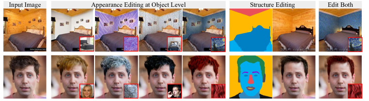
(a)

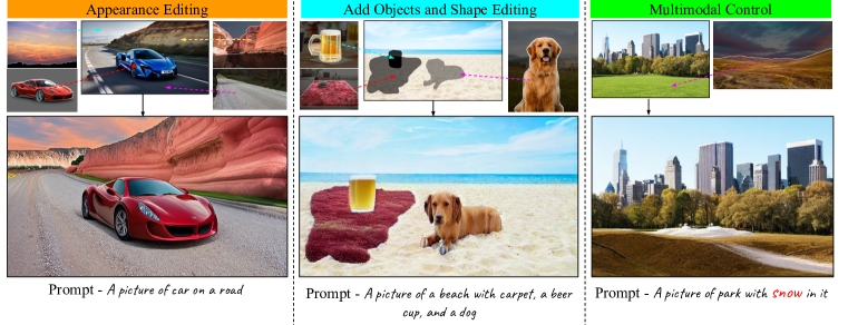
(b)

Figure 1: PAIR diffusion framework allows appearance and structure editing of an image at an object level. Our framework is general and can enable object-level editing capabilities in both (a) unconditional diffusion models and (b) foundational diffusion models. Using our framework with a foundational diffusion model allows for comprehensive in-the-wild object-level editing capabilities.

Diffusion-based generative models have shown promising results in synthesizing and manipulating images with great fidelity, among which text-to-image models and their follow-up works have great influence in both academia and industry. When editing a real image a user generally desires to have intuitive and precise control over different elements (i.e. the objects) composing the image in an independent manner. We can categorize existing image editing methods based on the level of control they have over individual objects in an image. One line of work involves the use of text prompts to manipulate images (Hertz et al., 2022; Liu et al., 2022; Brooks et al., 2022; Liew et al., 2022). These methods have limited capability for fine-grained control at the object level, owing to the difficulty of describing the shape and appearance of multiple objects simultaneously with text. In the meantime, prompt engineering makes the manipulation task tedious and time-consuming. Another line of work uses low-level conditioning signals such as masks Hu et al. (2022); Zeng et al. (2022b); Patashnik et al. (2023), sketches (Voynov et al., 2022), images (Song et al., 2022; Cao et al., 2023; Yang et al., 2023) to edit the images. However, most of these works either fall into the prompt engineering pitfall or fail to independently manipulate multiple objects. Different from previous works, we aim to independently control the properties of multiple objects composing an image i.e. object-level editing. We show that we can formulate various image editing tasks under the object-level editing framework leading to comprehensive editing capabilities.

To tackle the aforementioned task, we propose a novel framework, dubbed Structure-and-Appearance Paired Diffusion Models (PAIR-Diffusion). Specifically, we perceive an image as an amalgamation of diverse objects, each described by various factors such as shape, category, texture, illumination, and depth. Then we further identified two crucial macro properties of an object: structure and appearance. Structure oversees object’s shape and category, while appearance contains details like texture, color, and illumination. To accomplish this goal, PAIR-Diffusion adopts an off-the-shelf network to estimate panoptic segmentation maps as the structure, and then extract appearance representation using pre-trained image encoders. We use the extracted per-object appearance and structure information to condition a diffusion model and train it to generate images. In contrast to previous text-guided image editing works (Avrahami et al., 2022; Brooks et al., 2022; Couairon et al., 2022b; Ruiz et al., 2022), we consider an additional reference image to control the appearance. Compared to text prompts although convenient, they can only vaguely describe the appearance, images can precisely define the expected texture and make fine-grained image editing easier. Having the ability to control the structure and appearance of an image at an object level gives us comprehensive editing capabilities. Using our framework we can achieve, localized free-form shape editing, appearance editing, editing shape and appearance simultaneously, adding objects in a controlled manner, and object-level image variation (Fig. 1). Thanks to our design we do not require any inversion step for editing real images.

Our approach is general and can be used with various models. In this work, we show the efficacy of our framework on unconditional diffusion models and foundational text-to-image diffusion models. We also propose multimodal classifier-free guidance to reap the full benefits of the text-to-image diffusion models. It enables PAIR Diffusion to control the final output using both reference images and text in a controlled manner hence getting best of both worlds. Thanks to our easy-to-extract representations we do not require specialized datasets for training and we show results on LSUN datasets, Celeb-HQ datasets for unconditional models and use COCO datasets for foundational diffusion models. To summarize our contributions are as follows:

• We propose PAIR-Diffusion, a general framework to enable object-level editing in diffusion models. It allows editing the structure and appearance of each object in the image independently.

• The proposed design inherently supports various editing tasks using a single model: localized free-form shape editing, appearance editing, editing shape and appearance simultaneously, adding objects in a controlled manner, and object-level image variation.

• Additionally, we propose a multimodal classifier-free guidance that enables PAIR Diffusion to edit the images using both reference images and text in a controlled manner when using the approach with foundational diffusion models.

2 Related Works

Diffusion Models. Diffusion probabilistic models (Sohl-Dickstein et al., 2015) are a class of deep generative models that synthesize data through an iterative denoising process. Diffusion models utilize a forward process that applies noise into data distribution and then reverses the forward process to reconstruct the data itself. Recently, they have gained popularity for the task of image generation (Ho et al., 2020; Song & Ermon, 2019). Dhariwal et al.   Dhariwal & Nichol (2021) introduced various techniques such as architectural improvements and classifier guidance, that helped diffusion models beat GANs in image generation tasks for the first time. Followed by this, many works started working on scaling the models  (Nichol et al., 2021; Ramesh et al., 2022a; Rombach et al., 2022b; Saharia et al., 2022) to billions of parameters, improving the inference speed (Salimans & Ho, 2022) and memory cost (Rombach et al., 2022b; Vahdat et al., 2021). LDM (Rombach et al., 2022b) is one the most popular models which reduced the compute cost by applying the diffusion process to the low-resolution latent space and scaled their model successfully for text-to-image generation trained on webscale data. Other than image generation, they have been applied to various fields such as multi-modal generation (Xu et al., 2022b),text-to-3D (Poole et al., 2022; Singer et al., 2023), language generation (Li et al., 2022), 3D reconstruction (Gu et al., 2023), novel-view synthesis (Xu et al., 2022a), music generation (Mittal et al., 2021), object detection (Chen et al., 2022), etc.

Generative Image Editing. Image generation models have been widely used in image editing tasks since the inception of GANs (Karras et al., 2019; Jiang et al., 2021; Gong et al., 2019; Epstein et al., 2022; Ling et al., 2021), however, they were limited to edit a restricted set of images. Recent developments in the diffusion model has enabled image editing in the wild. Earlier works (Rombach et al., 2022a; Nichol et al., 2021; Ramesh et al., 2022b) started using text prompts to control the generated image. This led to various text-based image editing works such as (Feng et al., 2022; Mokady et al., 2022; Liu et al., 2022). To make localized edits works such as (Hertz et al., 2022; Parmar et al., 2023; Tumanyan et al., 2022) use cross-attention feature maps between text and image. InstructPix2Pix (Brooks et al., 2022) further enabled instruction-based image editing. However, using only text can only provide coarse edits. Works such as (Avrahami et al., 2022; Zeng et al., 2022a) explored explicit spatial conditioning to control the structure of generated images and used text to define the appearance of local regions. Works such as (Couairon et al., 2022a; Liew et al., 2022) rely on input images and text descriptions to get the region of interest for editing. However, most of the mentioned works lack object-level editing capabilities and some still rely only on text for describing the appearance. Recent works such as  (Mou et al., 2023; Epstein et al., 2023) have object-level editing capabilities, however, they are based on the classifier guidance technique at inference time which leads to limited precision. Further, they show results only on stable diffusion and require inversion to edit real images. Our framework is general and can be applied to any diffusion model. We also enable multimodal control of the appearances of objects in the image when using our framework with stable diffusion.

3 PAIR Diffusion

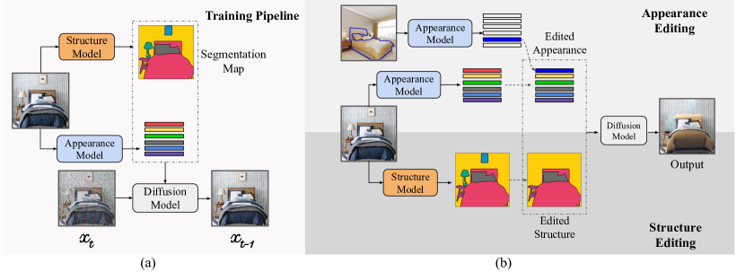
Figure 2: Overview of PAIR Diffusion. An image can be seen as a composition of objects each defined by different properties like structure (shape and category), appearance, depth, etc. We focus on controlling structure and appearance. (a) During training, we extract structure and appearance information and train a diffusion model in a conditional manner. (b) At inference, we can perform multiple editing operations by independently controlling the structure and appearance of any real image at the object level.

In this work, we aim to develop an image-editing framework that allows editing the properties of individual objects in the image. We perceive an image $x\in\displaystyle{\mathbb{R}}^{3\times H\times W}$ as composition of objects $\displaystyle{\mathbb{O}}=\{o_{1},o_{2},\dots o_{n}\}$ where $o_{i}$ represents the properties of $i^{th}$ object in the image. As discussed in Sec. 1, we focus on enabling control over the structure and the appearance of each object, hence we write $o_{i}=(s_{i},f_{i})$ where $s_{i}$ represents the structure, $f_{i}$ represents the appearance. Thus, the distribution that we aim to model can be written as

$$p(x|\displaystyle{\mathbb{O}},y)=p(x|\{(s_{1}\,f_{1}),\dots,(s_{n},\,f_{n})\},y)$$ (1)

We use $y$ to represent any form of conditioning signal already present in the generative model, e.g. text, and develop our framework to enable new object-level editing capabilities while preserving the original conditioning. The rest of the method section is organized as follows. In Sec.  3.1, we describe the method to obtain $s_{i}$ and $f_{i}$ for every object in a given image. Next, in Sec.  3.2, we show that various image editing tasks can be defined in the scope of the proposed object-level formulation of images. Finally, in Sec.  3.3, we describe the usage of the representations to augment the generative models and inference techniques to achieve object-level editing in practice.

3.1 Structure and Appearance Representation

Given an image $x\in\displaystyle{\mathbb{R}}^{3\times H\times W}$ we want to extract the structure and appearance of each object present in the image.

Structure: The structure oversees the object’s shape and category and is represented as $s_{i}=(c_{i},m_{i})$ where $c_{i}$ represents the category and $m_{i}\in\{0,1\}^{H\times W}$ represents the shape. We extract the structure information using a panoptic segmentation map, as it readily provides each object’s category and shape information and is easy to compute. Given an off the shelf segmentation network $E_{S}(\cdot)$, we obtain $\displaystyle{\bm{S}}=E_{S}(x)$, with $\displaystyle{\bm{S}}\in\mathbb{N}^{H\times W}$ which gives direct access to $c_{i},m_{i}$.

Appearance: The appearance representation is designed to capture the visual aspects of the object. To represent the object faithfully, it needs to capture both the low-level features like color, texture, etc., as well as the high-level features in the case of complex objects. To capture such a wide range of information, we choose a combination of convolution and transformer-based image encoders (Raghu et al., 2021), namely VGG (Simonyan & Zisserman, 2015) and DINOv2 (Oquab et al., 2023) to get appearance information. We use initial layers of VGG to capture low-level characteristics as they can capture details like color, texture etc. (Yosinski et al., 2015; Zeiler & Fergus, 2014). Conversely, DINOv2 has well-learned representations and has shown promising results for various downstream computer vision tasks. Hence, we use the middle layers of DINOv2 to capture the high-level characteristics of the object.

In order to compute per-object appearance representations, we first extract the feature maps from $l^{th}$ block of an encoder $E_{G}$, $\tilde{\displaystyle{\bm{\mathsfit{G}}}}=E^{l}_{G}(x)$ with $\tilde{\displaystyle{\bm{\mathsfit{G}}}}\in\mathbb{R}^{C\times h\times w}$, where $h\times w$ is the resulting spatial size, $C$ is the number of channels. We then parse object-level features, relying on $m_{i}$ to pool over the spatial dimension and obtain the appearance vector $\displaystyle{\bm{g}}^{l}_{i}\in\mathbb{R}^{C}$

$${\bm{g}}^{l}_{i}=\dfrac{\sum_{j,k}E^{l}_{G}(x)\odot m_{i}}{\sum_{j,k}{m_{i}}}$$ (2)

Here $E_{G}$ could be either DINOv2 or VGG. Let us use $\displaystyle{\bm{g}}^{Vl}_{i}$ and $\displaystyle{\bm{g}}^{Dl}_{i}$ to represent the appearance vectors extracted using features of VGG and DINOv2 at block $l$ respectively. The appearance information of $i^{th}$ object is given by a tuple $f_{i}=(\displaystyle{\bm{g}}^{Vl_{1}}_{i},\displaystyle{\bm{g}}^{Dl_{2}}_{i},\displaystyle{\bm{g}}^{Dl_{3}}_{i})$ where $l_{2}<l_{3}$. The abstraction level of features in $f_{i}$ increases from $\displaystyle{\bm{g}}^{Vl_{1}}_{s}$ to $\displaystyle{\bm{g}}^{Dl_{3}}_{s}$.

3.2 Image Editing Formulation

We can define various image editing tasks using the proposed object-level design. Consider an image $x$ with $n$ objects $\displaystyle{\mathbb{O}}=\{o_{1},o_{2},\dots o_{n}\}$. For each object $o_{i}$, we can extract $s_{i},f_{i}$ as described in Sec.  3.1. We present fundamental image editing operations below. The editing operations can be mixed with each other enabling a wide range of editing capabilities.

Appearance Editing $(s_{i},f_{i})\rightarrow(s_{i},f^{\prime}_{i})$. It can be achieved by simply swapping appearance vector $f_{i}$ with an edited appearance vector $f^{\prime}_{i}$. We can use the method described in Sec.  3.1 to extract the appearance vectors from reference images and use a convex combination of them to get $f^{\prime}_{i}$. Formally, $f^{\prime}_{i}=a_{0}f_{i}+a_{1}f^{R}_{i}$ where $f^{R}_{i}$ represents the appearance vectors of $i^{th}$ object in the reference image.

Shape Editing $(s_{i},f_{i})\rightarrow(s^{\prime}_{i},f_{i})$. It can be achieved by changing the structure $(c_{i},m_{i})$ to $(c_{i},m^{\prime}_{i})$ i.e. the shape can be explicitly changed by the user while maintaining the appearance.

Object Addition $\displaystyle{\mathbb{O}}\rightarrow\displaystyle{\mathbb{O}}\cup\{o_{n+1}\}$. We can add an object to an image by defining its structure and appearance. We can get them from a reference image or the user may give the structure and only appearance can come from a reference image.

Object Appearance Variation. We can also get object level appearance variations due to information loss when pooling features to calculate appearance vectors and the stochastic nature of the generative models.

Once we get object with edited properties $\displaystyle{\mathbb{O}}^{\prime}$ and conditioning $y$ we can sample a new image from the learned distribution $p(x|\displaystyle{\mathbb{O}}^{\prime},y)$. We can see that our object-level design can easily incorporate various editing abilities and help us achieve a comprehensive image editor. In the next section, we will describe a way to implement $p(x|\displaystyle{\mathbb{O}},y)$ in practice and inference methods to sample and control the edited image.

3.3 Architecture Design and Inference

In practice, Eq. 1 essentially represents a conditional generative model. Given the recent success of diffusion models, we use them to realize the Eq. 1. Our extracted representations in Sec. 3.1 can be used to enable object-level editing in any diffusion model. Here we briefly describe a method to use our represents on the unconditional diffusion models and foundational text-to-image (T2I) diffusion model. We start by representing structure and appearance in a spatial format to conveniently use them for conditioning. We represent the structure conditioning as $\displaystyle{\bm{\mathsfit{S}}}\in\mathbb{N}^{2\times H\times W}$ where the first channel has category information and the second channel has the shape information of each object. For appearance conditioning, we first $L2$ normalize each vector along channel dimension and splat them spatially using $m_{i}$ and combine them in a single tensor represented as $\displaystyle{\bm{\mathsfit{G}}}\in\mathbb{R}^{C\times H\times W}$ which leads to $F=(\displaystyle{\bm{\mathsfit{G}}}^{Vl_{1}},\displaystyle{\bm{\mathsfit{G}}}^{Dl_{2}},\displaystyle{\bm{\mathsfit{G}}}^{Dl_{3}})$. We then concatenate $\displaystyle{\bm{\mathsfit{S}}}$ to every element of $F$ which results in our final conditioning signals $F_{s}=(\displaystyle{\bm{\mathsfit{G}}}^{Vl_{1}}_{s},\displaystyle{\bm{\mathsfit{G}}}^{Dl_{2}}_{s},\displaystyle{\bm{\mathsfit{G}}}^{Dl_{3}}_{s})$.

In the case of the foundational T2I diffusion model, we choose Stable Diffusion (SD) (Rombach et al., 2022a) as our base model. In order to condition it, we adopt ControlNet (Zhang & Agrawala, 2023) because of its training and data efficiency in conditioning SD model. The control module consists of encoder blocks and middle blocks that are replicated from SD UNet architecture. There are various works that show in SD the inner layers with lower resolution tend to focus more on high-level features, whereas the outer layers focus more on low-level features (Cao et al., 2023; Tumanyan et al., 2022; Liew et al., 2022). Hence, we use $\displaystyle{\bm{\mathsfit{G}}}^{Vl_{1}}_{s}$ as input to the control module and add $\displaystyle{\bm{\mathsfit{G}}}^{Dl_{2}}_{s}$,$\displaystyle{\bm{\mathsfit{G}}}^{Dl_{3}}_{s}$ to the features after cross-attention in first and second encoder blocks of the control module respectively. For the unconditional diffusion model, we use the unconditional latent diffusion model (LDM) (Rombach et al., 2022a) as our base model. Pertaining to the simplicity of the architecture and training of these models we simply concatenate the features in $F_{s}$ to the input of LDM. The architecture is accordingly modified to incorporate the increased number of input channels. For further details please refer to Supp. Mat. .

For training both the models we follow standard practice (Rombach et al., 2022a) and use the simplified training objective $\mathcal{L}=||\epsilon-\epsilon_{\theta}(z_{t},\displaystyle{\bm{\mathsfit{S}}},F,y,t)||_{2}^{2}$ where $z_{t}$ represents the noisy version of $x$ in latent space at timestep $t$ and $\epsilon$ is the noise used to get $z_{t}$ and $\epsilon_{\theta}$ represents the model being trained. In the case of Stable Diffusion, $y$ represents the text prompts, whereas $y$ can be ignored in the case of the unconditional diffusion model.

Multimodal Inference. Having a trained model we need an inference method such that we can guide the strengths of various conditioning signals and control the edited image. Here, we take the case when $y$ is text and unconditional diffusion models would be a special case where $y$ is null. Specifically, the structure $\displaystyle{\bm{\mathsfit{S}}}$ and appearance $F$ come from a reference image and the information in $y$ could be disjoint from $F$, we need a way to capture both in the final image. A well-trained diffusion model estimates the score function of the underlying data distribution Song et al. (2020) i.e $\displaystyle\nabla_{z_{t}}p(z_{t}|\displaystyle{\mathbb{O}},y)=\displaystyle\nabla_{z_{t}}p(z_{t}|\displaystyle{\bm{\mathsfit{S}}},F,y)$, which in our case can be expanded as

$$\nabla_{z_{t}}\displaystyle\log p(z_{t}|\displaystyle{\bm{\mathsfit{S}}},F,y)=\displaystyle\nabla_{z_{t}}\displaystyle\log p(z_{t}|\displaystyle{\bm{\mathsfit{S}}},F)+\displaystyle\nabla_{z_{t}}\displaystyle\log p(z_{t}|y)-\displaystyle\nabla_{z_{t}}\displaystyle\log p(z_{t})$$ (3)

We use the concept of classifier-free guidance (CFG) Ho & Salimans (2022) to represent all score functions in the above equation using a single model by dropping the conditioning with some probability during training. Using the CFG formulation we get the following update rule from Eq. 3

$$\begin{split}\tilde{\epsilon_{\theta}}(z_{t},\displaystyle{\bm{\mathsfit{S}}},F,y)=\epsilon_{\theta}(z_{t},\phi,\phi,\phi)+s_{S}\cdot\left(\epsilon_{\theta}\left(z_{t},\displaystyle{\bm{\mathsfit{S}}},\phi,\phi\right)-\epsilon_{\theta}\left(z_{t},\phi,\phi,\phi\right)\right)\\ +s_{F}\cdot\left(\epsilon_{\theta}\left(z_{t},\displaystyle{\bm{\mathsfit{S}}},F,\phi\right)-\epsilon_{\theta}\left(z_{t},\displaystyle{\bm{\mathsfit{S}}},\phi,\phi\right)\right)+s_{y}\cdot\left(\epsilon_{\theta}\left(z_{t},\phi,\phi,y\right)-\epsilon_{\theta}(z_{t},\phi,\phi,\phi)\right)\end{split}$$ (4)

For brevity, we did not include $t$ in the equation above. A formal proof of the above equations is provided in Supp. Mat. . Intuitively, $F$ is more information-rich compared to $y$. Due to this, during training the network learns to give negligible importance to $y$ in the presence of $F$ and we need to use $y$ independently of $F$ during inference to see its effect on the final image. In Eq. 4 $s_{S},s_{F},s_{y}$ are guidance strengths for each conditioning signal. It provides PAIR Diffusion with an intuitive way to control and edit images using various conditions. For example, if a user wants to give more importance to a text prompt compared to the appearance from the reference image, it can set $s_{y}>s_{F}$ and vice-versa. For the unconditional diffusion models, we can simply ignore the term corresponding to $s_{y}$ in Eq 4.

4 Experiments

In this section, we present qualitative and quantitative analysis that show the advantages of the PAIR diffusion framework introduced in Sec. 3. We refer to UC-PAIR Diffusion to denote our framework applied to unconditional diffusion models and reserve the name PAIR Diffusion when applying the framework to Stable Diffusion. Evaluating image editing models is hard, moreover, there are few works that have comprehensive editing capabilities at the object level making a fair comparison even more challenging. For these reasons, we perform two main sets of experiments. Firstly, we train UC-PAIR Diffusion on widely used image-generation datasets such as the bedroom and church partitions of the LSUN Dataset (Yu et al., 2015), and the CelebA-HQ Dataset (Karras et al., 2017). We conduct quantitative experiments on these datasets as they represent a well-study benchmark, with a clear distinction between training and testing sets, making it easier and fairer to perform evaluations. Secondly, we fine-tune PAIR Diffusion on the COCO (Lin et al., 2014) dataset. We use this model to perform in-the-wild editing and provide examples for the use cases described in Sec. 3.2, showing the comprehensive editing capabilities of our method. We refer the reader to the Supp. Mat. for the details regarding model training and implementations, along with additional results.

4.1 Editing Applications

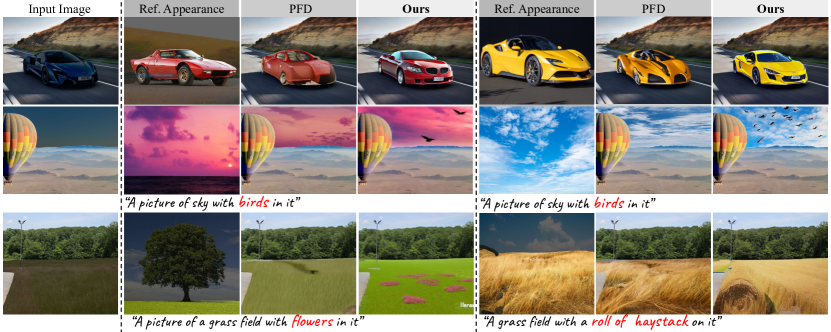
Figure 3: Qualitative results for appearance editing.

In this section, we qualitatively validate that our model can achieve comprehensive object-level editing capabilities in practice. We primarily show results using PAIR Diffusion and refer to the Supp. Mat. for results on smaller datasets. We use different baselines according to the editing task. We adapt Prompt-Free-Diffusion (PFD)  Xu et al. (2023) as a baseline for localized appearance editing, by introducing masking and using the cropped reference image as input. Moreover, we adopt Paint-By-Example (PBE) Yang et al. (2023) as a baseline for adding objects and shape editing. For further details regarding implementation please refer to Supp. Mat. . When we want the final output to be influenced by the text prompt as well we set $s_{y}>s_{F}$ else we set $s_{y}<s_{F}$. For the figures where there is no prompt provided below the image assume that prompt was auto-generated using the template A picture of {category of object being edited}. When editing a local region we used a masked sampling technique to only affect the selected region (Rombach et al., 2022a).

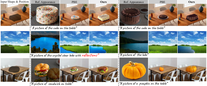
Figure 4: Qualitative results for adding objects and shape editing.

Appearance Editing. In Fig. 3, we report qualitative results for appearance editing driven by reference images and text. We can see that our multilevel appearance representation and object-level design help us edit the appearance of both simple objects such as the sky as well as complex objects like cars. On the other hand, PFD (Xu et al., 2023) gives poor results when editing the appearance of complex objects due to the missing object-level design. Furthermore, using our multimodal classifier free guidance, our model can seamlessly blend the information from the text and the reference images to get the final edited output whereas PFD (Xu et al., 2023) lacks this ability.

Add objects and Shape editing. We show the object addition and shape editing operations result together in Fig. 4. With PAIR Diffusion we can add complex objects with many details like a cake, as well as simpler objects like a lake. When changing the structure of the cake from a circle to a square, the model captures the sprinkles and dripping chocolate on the cake while rendering it in the new shape. In all the examples, we can see that the edges of the newly added object blend smoothly with the underlying image. On the other hand, PBE (Yang et al., 2023) completely fails to follow the desired shape and faces issues with large objects like lakes.

Variation. We can also achieve image variations at an object level as shown in Fig. 13 in Supp. Mat. . We can see that our model can capture various details of the original object and still produce variations.

4.2 Quantitative Results

Input	Reference	CP+Den.	E2EVE	PAIR-Diff

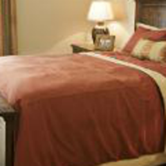
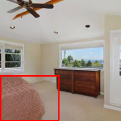
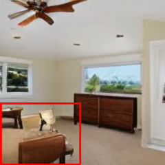
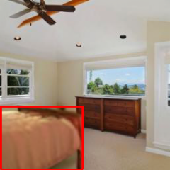
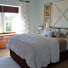
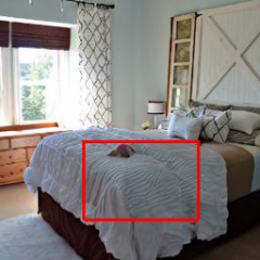
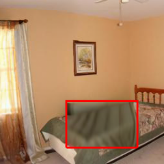
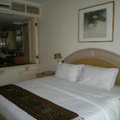
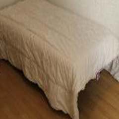
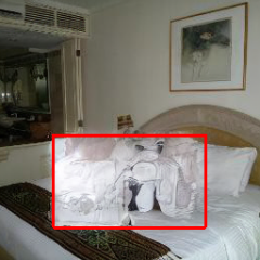
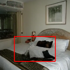
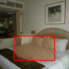
Figure 5: Visual results for appearance control on LSUN bedroom. We show the results obtained with relevant baselines for editing the red area in the input image using the reference as a driver.

Table 1: Quantitative results for appearance control on the LSUN Bedroom validation set.

Model	FID ($\downarrow$)	L1 ($\downarrow$)	SSIM ($\uparrow$)
Copy-Paste (CP)	21.37	0.0	0.87
Inpainting	8.25	0.02	0.17
CP+Denoise	9.15	0.02	0.32
E2EVE	13.59	0.05	0.34
PAIR-Diff	12.81	0.02	0.51

Table 2: Quantitative results for structure control on CelebA-HQ validation dataset.

Model	mIoU ($\uparrow$)	SSIM ($\uparrow$)
SEAN	0.64	0.32
PAIR-Diff	0.67	0.52

As described in Sec.3, the backbone of our design is the ability to control two major properties of the objects, the appearance and the structure. The aim of the quantitative evaluation is to verify that we can control the mentioned properties and not necessarily to push the state-of-the-art results. We start by evaluating our model on appearance control: the task consists of modifying a specific region of the input image using a reference image to drive the edit. We compare our method with the recent work of Brown et al. (2022) (E2EVE), and follow their evaluation procedure. In particular, different models are compared based on: (i) Naturalness: we expect the edited image to look realistic and rely on FID between input and edited images to assess it, (ii) Locality: we expect the edit to be limited to the specific region where the edit is performed and use L1 distance to measure it, (iii) Faithfulness: we expect the edited region and the target image to be similar and we use SSIM to evaluate it. As discussed in E2EVE, all the above-mentioned criteria should hold at the same time, and the best-performing method is the one giving good results in the three metrics at the same time. We compare our method with four baselines: (1) Copy-Paste: the driver image is simply copied in the edit region of the input image, (2) Inpainting: we use LDM Rombach et al. (2022b) to inpaint the target edit region, (3) Copy-Paste + Denoise: starting form copy-paste edit, we invert the image with DDIM, and denoise it with LDM, (4) E2EVE. In Tab. 2 we report the quantitative results on the validation set of LSUN Bedroom (Yu et al., 2015) and visual comparisons are shown in Fig.5. The copy-paste baseline provides an upper bound to the faithfulness and locality but produces images that are unrealistic (high FID score). Vice-versa, Inpainting and CP+Denoise produce natural results (low FID score) but are not faithful to the driver image (low SSIM score). Only our method performs well w.r.t. all the aspects and outperforms E2EVE in all metrics showing that we can control the appearance of a region. We refer the reader to Supp. Mat. for a detailed description of the evaluation procedure and baseline implementation.

Secondly, we evaluate the structure-controlling ability of our method. We adopt the validation set of CelebA-HQ (5000 samples) and compare with SEAN (Zhu et al., 2020). We generate images conditioning the model on the ground truth structure maps from the validation set and then segment the generated images with a pre-trained model zllrunning (2019). We report the mIoU score, calculated using the ground truth segmentation map as the reference, as well as the SSIM score in Table 2. The proposed method outperforms  Zhu et al. (2020) in terms of both mIoU and SSIM, demonstrating that our method can precisely follow the guidance of structure and retain the appearance.

4.3 Ablation Study

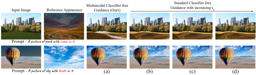
Figure 6: Ablation study for multimodal classifier-free guidance. We can see that if we use standard classifier-free guidance (Eq. 5) the model completely ignores the text when sampling the image.

Multimodal Classifier Free Guidance. Here we validate the effectiveness of the proposed multimodal classifier-free guidance. Instead of factorizing which results in Eq. 3 we directly expand the conditional score function $\displaystyle\nabla_{z_{t}}\displaystyle\log p(z_{t}|\displaystyle{\bm{\mathsfit{S}}},F,y)$ and apply classifier free guidance formulation on it and get the following equation.

$$\begin{split}\tilde{\epsilon_{\theta}}(z_{t},\displaystyle{\bm{\mathsfit{S}}},F,y)=\epsilon_{\theta}(z_{t},\phi,\phi,\phi)+s_{S}\cdot\left(\epsilon_{\theta}\left(z_{t},\displaystyle{\bm{\mathsfit{S}}},\phi,\phi\right)-\epsilon_{\theta}\left(z_{t},\phi,\phi,\phi\right)\right)\\ +s_{F}\cdot\left(\epsilon_{\theta}\left(z_{t},\displaystyle{\bm{\mathsfit{S}}},F,\phi\right)-\epsilon_{\theta}\left(z_{t},\displaystyle{\bm{\mathsfit{S}}},\phi,\phi\right)\right)\color[rgb]{0,0,1}+s_{y}\cdot\left(\epsilon_{\theta}\left(z_{t},{\bm{\mathsfit{S}}},F,y\right)-\epsilon_{\theta}(z_{t},{\bm{\mathsfit{S}}},F,\phi)\right)\end{split}$$ (5)

We highlight the difference between Eq. 4 and Eq. 5 using blue color. We compare the results sampled from Eq. 4 and Eq. 5 in Fig. 6. In the figure, column (a) shows results from Eq. 4 whereas column (b) - (d) shows results from Eq. 5 with increasing $s_{y}$. We use the same seed to generate all the images, further the values of $s_{S},s_{F},s_{y}$ are the same in columns (a) and (b). For the first row we set $s_{S}=8,s_{F}=3,s_{y}=8$ and for second row it is $s_{S}=6,s_{F}=4,s_{y}=8$. The values of $s_{y}$ for (b) - (d) are $8,15,20$ respectively. We can clearly see that sampling results using Eq. 5 completely fail to take text prompt into consideration even after increasing the value of $s_{y}$. This shows the effectiveness of the proposed classifier-free guidance Eq. 4 for controlling the image in a multimodal manner.

Appearance representation. We ablate the importance of using both VGG and DINOv2 for representing the appearance of an object. We train two models, one using only VGG features for appearance and the second using only DINOv2 features for appearance and are represented using $M_{VGG}$ and $M_{DINO}$ respectively. We trained two models using exactly the same hyperparameters as our original model.

Table 3: Quantitative results of ablation study on appearance representation

Model	L1 $\downarrow$	LPIPS $\downarrow$
$M_{VGG}$	0.1893	0.555
$M_{DINO}$	0.1953	0.549
Ours	0.1891	0.545

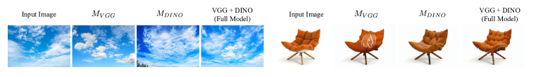
Figure 9: Object level appearance variations are shown for models trained with different appearance representations. It can be observed that $M_{DINO}$ faces difficulty in preserving the color when generating variations. The sky is a bit darker than the input image whereas, in the case of the couch, the shade of orange color does not match the input image. We can see that $M_{VGG}$ is able to preserve the color however it can have artifacts even for slightly complex objects. In the case of the couch, we can see some white artifacts that might have come from the white bottom of the couch in the input image. $M_{VGG}$ have a poor understanding of objects compared to $M_{DINO}$. Only the full model which uses both captures the visual aspects of the object faithfully.

We validate it using pairwise image similarity metrics on the COCO validation dataset. We use L1 as our low-level metric and LPIPS (Zhang et al., 2018) as our high-level metric, results are shown in Tab. 3. We can see that $M_{VGG}$ has a better L1 score compared to $M_{DINO}$ whereas LPIPs score is better for $M_{DINO}$ compared to $M_{VGG}$. This shows that VGG features are good at capturing low-level details and DINO features are good at capturing high-level details in our design. When we use both features together we get the best L1 and LPIPS score getting the best of both of the features. Hence, in our final design, we used both VGG and DINOv2 features for appearance vectors. Supporting visuals can be found in Fig 9.

5 Conclusion

In this paper, we showed that we can build a comprehensive image editor by leveraging the observation that images are amalgamations of various objects. We proposed a generic framework dubbed PAIR Diffusion that enables structure and appearance editing at object-level editing in any diffusion model. Our proposed framework enables various object-level editing operations on real images without the need for inversion such as appearance editing, structure editing, adding objects, and variations all of which can be done by training the model only once. We also proposed multimodal classifier-free guidance which enables multimodal control in the editing operations when using our framework with models like stable diffusion. We validated the efficacy of the framework by showing extensive editing results using our model on diverse domains of real images. In the future, one can also explore the design of appearance vectors such that we can further control the illumination, pose, etc, and have better identity preservation of the object being edited. We hope that our work motivates future works to move in the direction of object-level image editing which might help to formulate and build an all-in-one image editing model.

Appendix

This appendix contains three sections organized as follows. In Sec.A we discuss our proposed multimodal classifier free guidance, proving Eq. 4 of the main paper and providing qualitative results for its usage. In Sec. B, we report the implementation details of our unconditional model along with details about the baselines adopted in the paper. Lastly, in Sec. C we show additional qualitative results and applications of our framework.

Appendix A Multimodal Classifier Free Guidance

A.1 Proof

Let us represent $p(z|c)$ as the distribution we want to learn where $c$ is $\displaystyle{\bm{\mathsfit{S}}},F,y$. Here $z$ represents $x$ in latent space. A well-trained diffusion model learns to estimate $\displaystyle\nabla_{z_{t}}\displaystyle\log p(z_{t}|c)$. Let us focus on $\displaystyle\log p(z_{t}|c)$. Using Bayes’s rule and taking log

$$\log p(z_{t}|c)=\displaystyle\log p(c|z_{t})+\displaystyle\log p(z_{t})-\displaystyle\log p(c)$$ (6)

In our setting of multimodal inference, we want to affect the final image using the appearance from the reference image $F$ and the text prompt $y$ independently. Multimodal inference would be particularly useful when the information in $y$ would be disjoint from $\displaystyle{\bm{\mathsfit{S}}},F$ and we need to capture it in the final image. Using this we can write.

$$\begin{split}\displaystyle\log p(\displaystyle{\bm{\mathsfit{S}}},F,y)=\displaystyle\log p(\displaystyle{\bm{\mathsfit{S}}},F)+\displaystyle\log p(y)\end{split}$$ (7)

Now expanding $\displaystyle\log p(c|z_{t})$ and using Eq 7

$$\begin{split}\displaystyle\log p(c|z_{t})&=\displaystyle\log p(\displaystyle{\bm{\mathsfit{S}}},F,y|z_{t})\\ \displaystyle\log p(\displaystyle{\bm{\mathsfit{S}}},F,y|z_{t})&=\displaystyle\log p(\displaystyle{\bm{\mathsfit{S}}},F|z_{t})+\displaystyle\log p(y|z_{t})\end{split}$$ (8)

Plugging the Eq. 8 in Eq. 6 and using Eq. 7 again we get

$$\begin{split}\displaystyle\log p(z_{t}|\displaystyle{\bm{\mathsfit{S}}},F,y)&=\displaystyle\log p(\displaystyle{\bm{\mathsfit{S}}},F|z_{t})+\displaystyle\log p(y|z_{t})+\displaystyle\log p(z_{t})-\displaystyle\log p(\displaystyle{\bm{\mathsfit{S}}},F,y)\\ \displaystyle\log p(z_{t}|\displaystyle{\bm{\mathsfit{S}}},F,y)&=\displaystyle\log p(\displaystyle{\bm{\mathsfit{S}}},F|z_{t})+\displaystyle\log p(y|z_{t})+\displaystyle\log p(z_{t})-\displaystyle\log p(\displaystyle{\bm{\mathsfit{S}}},F)-\displaystyle\log p(y)\\ \displaystyle\log p(z_{t}|\displaystyle{\bm{\mathsfit{S}}},F,y)&=\displaystyle\log p(z_{t}|\displaystyle{\bm{\mathsfit{S}}},F)+\displaystyle\log p(z_{t}|y)-\displaystyle\log p(z_{t})\end{split}$$ (9)

Taking gradient w.r.t. $\displaystyle\nabla_{z_{t}}$ we can get

$$\nabla_{z_{t}}\displaystyle\log p(z_{t}|\displaystyle{\bm{\mathsfit{S}}},F,y)=\displaystyle\nabla_{z_{t}}\displaystyle\log p(z_{t}|\displaystyle{\bm{\mathsfit{S}}},F)+\displaystyle\nabla_{z_{t}}\displaystyle\log p(z_{t}|y)-\displaystyle\nabla_{z_{t}}\displaystyle\log p(z_{t})$$ (10)

Applying baye’s rule to $\displaystyle\nabla_{z_{t}}\displaystyle\log p(z_{t}|\displaystyle{\bm{\mathsfit{S}}},F)$ and $\displaystyle\nabla_{z_{t}}\displaystyle\log p(z_{t}|y)$

$$\begin{split}\displaystyle\nabla_{z_{t}}\displaystyle\log p(z_{t}|\displaystyle{\bm{\mathsfit{S}}},F)=\displaystyle\nabla_{z_{t}}\displaystyle\log p(F|\displaystyle{\bm{\mathsfit{S}}},z_{t})+\displaystyle\nabla_{z_{t}}\displaystyle\log p(S|z_{t})+\displaystyle\nabla_{z_{t}}\displaystyle\log p(z_{t})-\cancelto{0}{\displaystyle\nabla_{z_{t}}\displaystyle\log p(\displaystyle{\bm{\mathsfit{S}}},F)}\end{split}$$ (11)

$$\begin{split}\displaystyle\nabla_{z_{t}}\displaystyle\log p(z_{t}|y)=\displaystyle\nabla_{z_{t}}\displaystyle\log p(y|z_{t})+\displaystyle\nabla_{z_{t}}\displaystyle\log p(z_{t})-\cancelto{0}{\displaystyle\nabla_{z_{t}}\displaystyle\log p(y)}\end{split}$$ (12)

Pluggin Eq. 11 and Eq. 12 in Eq. 10 we get

$$\begin{split}\displaystyle\nabla_{z_{t}}\displaystyle\log p(z_{t}|\displaystyle{\bm{\mathsfit{S}}},F,y)=\displaystyle\nabla_{z_{t}}\displaystyle\log p(F|\displaystyle{\bm{\mathsfit{S}}},z_{t})+\displaystyle\nabla_{z_{t}}\displaystyle\log p(S|z_{t})+\displaystyle\nabla_{z_{t}}\displaystyle\log p(y|z_{t})+\displaystyle\nabla_{z_{t}}\displaystyle\log p(z_{t})\end{split}$$ (13)

We can use the concept of classifier-free-guidance Ho & Salimans (2022) to approximate the above equation using a single model which has been trained by dropping the conditions during training and get the final sampling equation Eq. 4

$$\begin{split}\tilde{\epsilon_{\theta}}(z_{t},\displaystyle{\bm{\mathsfit{S}}},F,y)=\epsilon_{\theta}(z_{t},\phi,\phi,\phi)+s_{S}\cdot\left(\epsilon_{\theta}\left(z_{t},\displaystyle{\bm{\mathsfit{S}}},\phi,\phi\right)-\epsilon_{\theta}\left(z_{t},\phi,\phi,\phi\right)\right)\\ +s_{F}\cdot\left(\epsilon_{\theta}\left(z_{t},\displaystyle{\bm{\mathsfit{S}}},F,\phi\right)-\epsilon_{\theta}\left(z_{t},\displaystyle{\bm{\mathsfit{S}}},\phi,\phi\right)\right)+s_{y}\cdot\left(\epsilon_{\theta}\left(z_{t},\phi,\phi,y\right)-\epsilon_{\theta}(z_{t},\phi,\phi,\phi)\right)\end{split}$$ (14)

A.2 Ablation on CFG control parameters

The multimodal classifier free guidance has three control parameters namely $s_{S},s_{F},s_{y}$. In practice, the values $s_{S},s_{F},s_{y}$ can be understood as the guidance strengths to control how the final image is affected by the structure, reference image, and the given text prompt. When using it to edit real-world images it is crucial to understand how they change the output image when varied together. In this section, we study the effect of (a) varying structure guidance $s_{S}$ and reference image guidance $s_{F}$ (b) varying text prompt guidance $s_{y}$ and reference image guidance $s_{F}$.

Structure ($s_{s}$) and Appearance ($s_{F}$). We explain the importance of parameters by choosing a reference image that is completely different from the underlying structure in the input image. The results are shown in Fig. 7. We can observe that as we increase $s_{F}$ the model forcefully imposes the reference image appearance on the object being edited and the object starts losing its structural integrity. We can get back the structural integrity when increasing $s_{S}$ as well. Notice, in the second row, when $s_{F}=4$ and $s_{S}=2$ we cannot see any parts of the car such as the wheel, headlight, windshield, etc. When we start increasing $s_{S}$ the subpart of the car starts appearing the edited region starts looking more like a car. However, when we increase $s_{F}$ too much as in the last row, even after increasing $s_{S}$ does not help much. In general, it is good practice to keep $s_{S}>s_{F}$ when editing real images. Further, we can adjust $s_{F}$ how closely we want the edited output to follow the reference appearance.

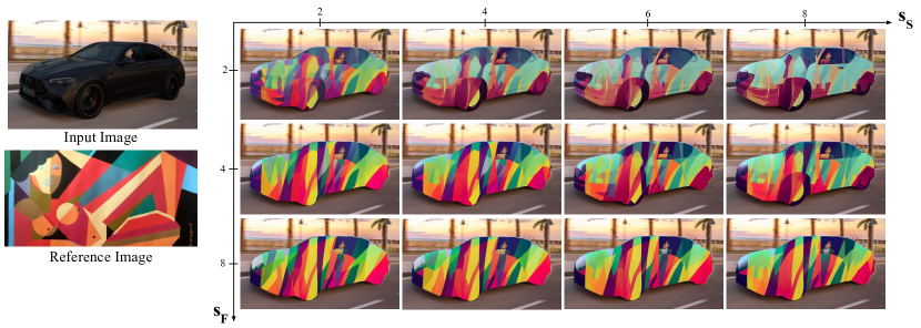
Figure 7: The figure shows the affect of $s_{F}$ and $s_{S}$ parameter in multimodal classifier free guidance Eq. 4 when they are varied. We can see that as we increase $s_{F}$ the output forcefully imposes the appearance from the reference image and the car starts losing the structure details that were helping to make it look like a car. We need to increase $s_{S}$ as well to maintain the structural integrity of the car. However, when we increase $s_{F}$ too much even after increasing $s_{S}$ does not help much.

Text Prompt ($s_{y}$) and Appearance ($s_{F}$): Here we try to analyze the effect of two crucial guidance parameters which help us in controlling and editing images in a multimodal manner. The results are shown in Fig 8. We can see that it is crucial to keep $s_{y}>s_{F}$ to see the effects of the text prompt on the output image. Further, we can see that the model is more sensitive to the $s_{F}$ parameter compared to $s_{y}$. Even if we increase $s_{F}$ slightly we can see diminishing effects of the prompt on the edited image. In general when editing images in a multimodal manner it is a good practice to keep $s_{y}>s_{F}$ and $s_{F}$ should have a low value in an absolute sense. Keeping these constraints we can vary the parameters to adjust the final output as per the need.

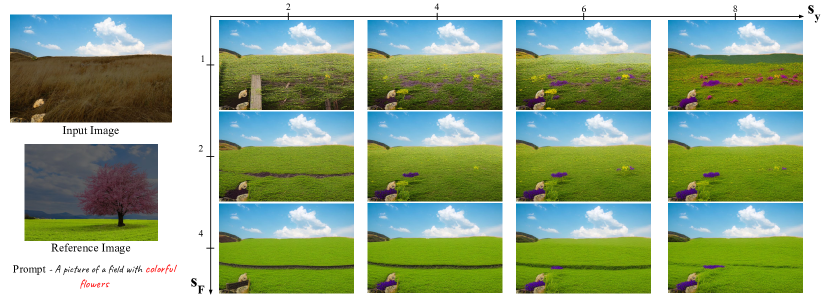
Figure 8: The figure shows the effect of $s_{F}$ and $s_{T}$ parameter in multimodal classifier free guidance Eq. 4 when they are varied. $s_{F}$ controls the effect of the reference image and $s_{y}$ control the effect of the prompt. We can see that the output is highly sensitive to $s_{F}$. Even if we increase $s_{F}$ slightly the effect of the prompt starts disappearing. When we want to use both reference images and prompts to affect the final image it is best to keep $s_{y}>s_{F}$ and $s_{F}$ should have a low value in an absolute sense.

Appendix B Implementation Details

B.1 PAIR Diffusion

Unconditional Diffusion Model. In this section, we provide additional details for implementing PAIR Diffusion framework on unconditional diffusion models. We used LDM Rombach et al. (2022a) as our base architecture and trained on LSUN Church, Bedroom, and CelebA-HQ datasets. To extract the structure information, we apply SeMask-L Jain et al. (2021) with Mask2former Cheng et al. (2022) trained on ADE20K Zhou et al. (2017), and compute the segmentation mask for LSUN Church and Bedroom datasets Yu et al. (2015). In CelebA-HQ, ground truth segmentation masks are available. Pertaining to the simplicity of the architecture and training datasets of these models we found that simply using $\displaystyle{\bm{\mathsfit{G}}}^{Vl_{1}}$ as appearance vectors is sufficient to achieve various editing capabilities. For conditioning, we simply concatenate $\displaystyle{\bm{\mathsfit{G}}}^{Vl_{1}}$ to the noisy latent $z_{t}$ along the channels dimension. We increase the number of channels of the first convolutional layer of the U-Net from $C_{in}$ to $C_{in}+C+1$ and keep the rest of the architecture as in Rombach et al. (2022b). Here $C$ is the number of channels in $\displaystyle{\bm{\mathsfit{G}}}^{Vl_{1}}$ where $l_{1}=1$. For all three datasets namely, LSUN Church, Bedroom, and CelebA-HQ we start with the pre-trained weights provided by LDM Rombach et al. (2022b) and finetune with exactly the same hyperparameters mentioned in the paper Rombach et al. (2022b). The number of steps, learning rate, and batch size are reported in Tab 4. We train our models using A100 GPUs. During training, we randomly dropped structure and appearance conditioning with a probability of $10\%$. At inference time, we adapt Eq. 4 for sampling from the model by setting $s_{y}=0$ and use classifier-free guidance style sampling using the DDIM algorithm Song & Ermon (2019) with 250 steps.

Base Model	Dataset	lr	batch size	Iterations	GPU Days
LDM	Bedroom	9.6e-5	48	750k	24
LDM	Churches	1.0e-5	96	350k	12
LDM	CelebA-HQ	9.6e-5	24	120k	1
SD + ControlNet	COCO	1.5e-5	128	86k	96

Table 4: Hyperparameters for PAIR diffusion when used with LDM Rombach et al. (2022a) and SD + ControlNet Zhang & Agrawala (2023).

Foundational Diffusion Model. We use Stable Diffusion (SD) Rombach et al. (2022a) as our base architecture and ControlNet Zhang & Agrawala (2023) to efficiently condition SD. We use COCO Caesar et al. (2018) dataset for the experiments and it already contains panoptic segmentation masks and image captions. In vanilla ControlNet, the conditioning signal is passed through a zero convolution network and added to the input noise after being passed through the first encoder block of the control module. We use $\displaystyle{\bm{\mathsfit{G}}}^{Vl_{1}}_{s}$ in a similar manner and use it as input to the control module as in vanilla ControlNet. Further, we modulate the features in the first encoder block of the control module using $\displaystyle{\bm{\mathsfit{G}}}^{Dl_{2}}$ and in the second encoder block using $\displaystyle{\bm{\mathsfit{G}}}^{Dl_{3}}$ by adding them to the respective features after cross-attention blocks. Before adding ${\bm{\mathsfit{G}}}^{Dl_{2}},{\bm{\mathsfit{G}}}^{Dl_{3}}$ we pass them through two linear layers to match the dimension of the features of the network. We train the network as described in ControlNet Zhang & Agrawala (2023) and only train the control module and the linear layers, while all the other parameters are frozen. We found that the combination $l_{1}=1,l_{2}=6,l_{3}=18$ worked best after performing grid search. During training, we randomly dropped structure, appearance, and text conditioning with a probability of $10\%$. Our model is trained across 4 A100 machines with 8 GPUs each and took 3 days to train the model. The number of steps, learning rate, and batch size are reported in Tab 4. At inference time, we apply Eq. 4 for sampling and use classifier-free guidance style sampling using the DDIM algorithm Song & Ermon (2019) with 20 steps.

B.2 Baselines

Quantitative Experiments. We provide additional details about implementation and evaluation procedures for the results shown in Sec. 4.2 of the main paper. We evaluate the models on the task of in-domain appearance manipulation. We first describe the data-collection procedure. We use 5000 images from the validation set of LSUN Bedroom, and choose the bed as the object to edit. For each image, we randomly select a patch within the bed, and use a patch extracted in the same way from another image as the driver for the edit. Next, we describe the baselines. Copy-Paste: The target patch is copied and pasted in the target region of the input image, resizing the patch to fit the target region. Inpainting, we use the model pretrained on LSUN Bedroom Dataset by Rombach et al. (2022b), and use it to inpaint the edit region. To do that, we use a masked sampling technique, as done in the inpainting task in  Rombach et al. (2022a). CP+Denoise, we start from the results of copy-paste and apply DDIM Inversion to map the image to the diffusion noise space Song & Ermon (2019). Subsequently, we apply LDM to denoise the image to the final result. Lastly, we compare our method with E2EVE Brown et al. (2022). We use the original pre-trained weights shared by the authors and use their model to perform the edit. Next, we detail the metrics calculation pipeline. We compute naturalness by measuring the FID between the edited images and the original images from the whole dataset. We estimate the locality, by measuring the L1 loss between the original image and the edited image outside the edited region (i.e. the region that should not change). Finally, the faithfulness is measured by the SSIM between the driver image and the edited region in the edited image.

Qualitative Experiments. We run Prompt-Free-Diffusion Xu et al. (2023) following the description in Sec. 4.5 of the paper and the github issue https://github.com/SHI-Labs/Prompt-Free-Diffusion/issues/3#issuecomment-1573091747. Specifically, we crop the input image around the object being edited and the reference image around the selected object. We feed the two crops to the SeeCoder, and use the segmentation ControlNet with the segmentation map of the cropped input image as the conditioning signal. We then get the edited image by cutting the region of interest in the output image and pasting it in the input image. Regarding Paint-By-Example Yang et al. (2023), we crop the reference image around the selected object and follow the original inference procedure afterward.

Appendix C Qualitative Results

C.1 Stable Diffusion Results

In this section, we show additional results for PAIR-Diffusion when coupled with a foundational diffusion model like Stable Diffusion Rombach et al. (2022b). In Fig. 11, we perform appearance manipulation in the wild, showing realistic edits in different scenarios. In Fig. 12, we provide additional results for the task of adding a new object to a given scene. Lastly, we showcase another capability of our model, producing variations of a given object. Specifically, we sample different initial latent codes $z_{i}\sim\mathcal{N}(0,1)$, while fixing the structure and appearance representation. We report the results in Fig. 13.

C.2 Unconditional PAIR Diffusion

We start by providing additional results for the task of appearance control. In Fig. 10 (a), we can notice that our method can easily transfer the appearance of a church from a completely different structure in the reference image to the structure of the church in the input image. At the same time, we can copy relatively homogeneous regions like the sky, transferring the color accurately, as well as more textured objects such as the trees. In Fig. 10 (b), it is interesting to note that, when we change the style of the floor, the model can appropriately place the reflections hence realistically harmonizing the edit with the rest of the scene. Similar observations can be made when we edit the wall. Lastly, in Fig. 10 (c) we show results on faces. We can observe that our method accurately transfers the appearance from the reference image, modifying the skin, hair, and eyebrows of the input. We notice that all our edits do not alter the identity of the person in the input image, which is a desirable property when editing faces.

Input	Building		Sky		Tree
(a)
Input	Bed		Wall		Floor
(b)
Input	Skin		Hair		Eyebrows
(c)

Figure 10: Qualitative results on In Domain Appearance Manipulation. Reference images are shown in the bottom right, while the text on top indicates the object targeted by the editing operation.

Next, we provide an additional qualitative comparison for the task of appearance control with the baselines detailed in Sec.B. In Fig. 14, we can observe that our method seamlessly transfers the appearance from the reference image to the input image, while maintaining the edit to the targeted region. Moreover, we show the qualitative comparison with SEAN Zhu et al. (2020) in Fig. 15. We can see that our method gives better editing results and we also allow to control the strength of the edit.

In Fig. 16, we showcase more nuanced appearance editing results instead of simply swapping the appearance of input and reference images (i.e. $f^{\prime}_{i}=f_{i}^{R}$) by linearly combining the two. We exploit the flexibility of our formulation by setting $a_{0}=\lambda,a_{1}=1-\lambda$, with $\lambda\in[0,1]$, i.e.  interpolating input and reference images. We can notice how the appearance of the edited region smoothly transitions from the original appearance to the reference, providing an additional level of control for the end user.

Lastly, we present a more challenging editing scenario using reference images that contain no semantics (e.g. abstract paintings) and use it to perform both localized and global editing in Fig. 17.

Input	Reference Appearance	PAIR-Diffusion

Figure 11: Appearance editing in the wild.

Input	Reference Appearance	PAIR-Diffusion

Figure 12: Add objects to the scene.

Input	Variations

Figure 13: Variations.

Input	Reference	CP	Inpaint	CP+DDIM	E2EVE	Our

Figure 14: Visual results for in-domain localized image editing. We edit the input image, using as driver the reference image, targeting the red-boxed area. With PAIR-Diffusion we can perform realistic edits in challenging scenarios. For example, in the first row, we can use the entire bed as a driver and edit only a patch of the input image. On the contrary, in the last row, we use a small patch as driver and target the whole bed of the input image for the edit. In both cases, our method outputs realistic edited images. Moreover, due to the masked DDIM technique we introduce almost no distortion in the area outside the red box (i.e. the one that should not change). We show results for all the baselines.

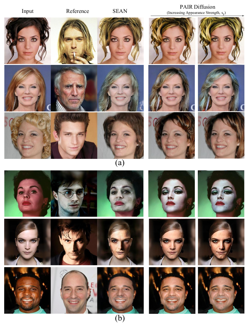
Figure 15: Comparison with SEAN.

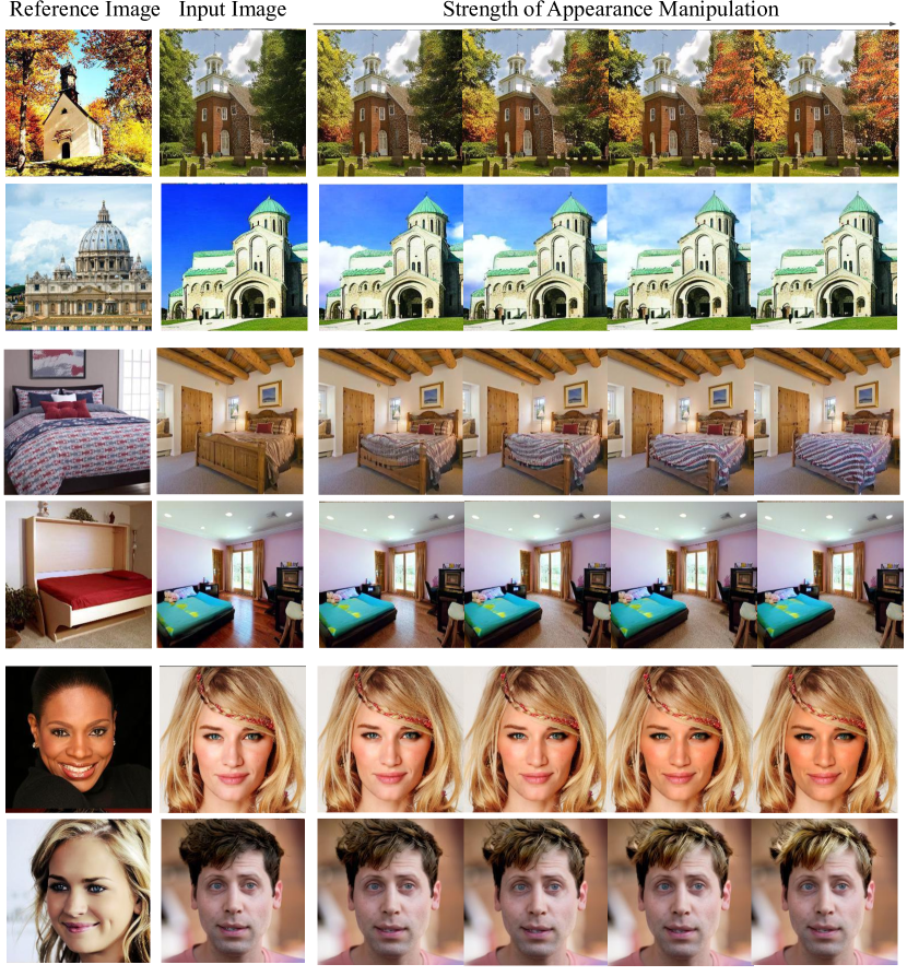
Figure 16: Interpolation results.

Input	Wall		Bed
Input	Church		Sky
(a)
(b)

Figure 17: Visual results for (a) local image editing, (b) global image appearance manipulation.

References

- Avrahami et al. (2022) Omri Avrahami, Thomas Hayes, Oran Gafni, Sonal Gupta, Yaniv Taigman, Devi Parikh, Dani Lischinski, Ohad Fried, and Xi Yin. SpaText: Spatio-Textual Representation for Controllable Image Generation, November 2022. URL http://arxiv.org/abs/2211.14305. arXiv:2211.14305 [cs].
- Brooks et al. (2022) Tim Brooks, Aleksander Holynski, and Alexei A Efros. Instructpix2pix: Learning to follow image editing instructions. arXiv preprint arXiv:2211.09800, 2022.
- Brown et al. (2022) Andrew Brown, Cheng-Yang Fu, Omkar Parkhi, Tamara L. Berg, and Andrea Vedaldi. End-to-end visual editing with a generatively pre-trained artist. In European Conference on Computer Vision (ECCV), 2022.
- Caesar et al. (2018) Holger Caesar, Jasper Uijlings, and Vittorio Ferrari. Coco-stuff: Thing and stuff classes in context. In Proceedings of the IEEE conference on computer vision and pattern recognition, pp. 1209–1218, 2018.
- Cao et al. (2023) Mingdeng Cao, Xintao Wang, Zhongang Qi, Ying Shan, Xiaohu Qie, and Yinqiang Zheng. Masactrl: Tuning-free mutual self-attention control for consistent image synthesis and editing. arXiv preprint arXiv:2304.08465, 2023.
- Chen et al. (2022) Shoufa Chen, Peize Sun, Yibing Song, and Ping Luo. Diffusiondet: Diffusion model for object detection. arXiv preprint arXiv:2211.09788, 2022.
- Cheng et al. (2022) Bowen Cheng, Ishan Misra, Alexander G Schwing, Alexander Kirillov, and Rohit Girdhar. Masked-attention mask transformer for universal image segmentation. In Proceedings of the IEEE/CVF conference on computer vision and pattern recognition, pp. 1290–1299, 2022.
- Couairon et al. (2022a) Guillaume Couairon, Jakob Verbeek, Holger Schwenk, and Matthieu Cord. Diffedit: Diffusion-based semantic image editing with mask guidance. arXiv preprint arXiv:2210.11427, 2022a.
- Couairon et al. (2022b) Guillaume Couairon, Jakob Verbeek, Holger Schwenk, and Matthieu Cord. DiffEdit: Diffusion-based semantic image editing with mask guidance, October 2022b. URL http://arxiv.org/abs/2210.11427. arXiv:2210.11427 [cs].
- Dhariwal & Nichol (2021) Prafulla Dhariwal and Alexander Nichol. Diffusion models beat gans on image synthesis. Advances in Neural Information Processing Systems, 34:8780–8794, 2021.
- Epstein et al. (2022) Dave Epstein, Taesung Park, Richard Zhang, Eli Shechtman, and Alexei A Efros. Blobgan: Spatially disentangled scene representations. In Computer Vision–ECCV 2022: 17th European Conference, Tel Aviv, Israel, October 23–27, 2022, Proceedings, Part XV, pp. 616–635. Springer, 2022.
- Epstein et al. (2023) Dave Epstein, Allan Jabri, Ben Poole, Alexei A Efros, and Aleksander Holynski. Diffusion self-guidance for controllable image generation. arXiv preprint arXiv:2306.00986, 2023.
- Feng et al. (2022) Weixi Feng, Xuehai He, Tsu-Jui Fu, Varun Jampani, Arjun Akula, Pradyumna Narayana, Sugato Basu, Xin Eric Wang, and William Yang Wang. Training-free structured diffusion guidance for compositional text-to-image synthesis. arXiv preprint arXiv:2212.05032, 2022.
- Gong et al. (2019) Xinyu Gong, Shiyu Chang, Yifan Jiang, and Zhangyang Wang. Autogan: Neural architecture search for generative adversarial networks. In Proceedings of the IEEE/CVF International Conference on Computer Vision, pp. 3224–3234, 2019.
- Gu et al. (2023) Jiatao Gu, Alex Trevithick, Kai-En Lin, Josh Susskind, Christian Theobalt, Lingjie Liu, and Ravi Ramamoorthi. Nerfdiff: Single-image view synthesis with nerf-guided distillation from 3d-aware diffusion. arXiv preprint arXiv:2302.10109, 2023.
- Hertz et al. (2022) Amir Hertz, Ron Mokady, Jay Tenenbaum, Kfir Aberman, Yael Pritch, and Daniel Cohen-Or. Prompt-to-prompt image editing with cross attention control. arXiv preprint arXiv:2208.01626, 2022.
- Ho & Salimans (2022) Jonathan Ho and Tim Salimans. Classifier-Free Diffusion Guidance, July 2022. URL http://arxiv.org/abs/2207.12598. arXiv:2207.12598 [cs].
- Ho et al. (2020) Jonathan Ho, Ajay Jain, and Pieter Abbeel. Denoising diffusion probabilistic models. Advances in Neural Information Processing Systems, 33:6840–6851, 2020.
- Hu et al. (2022) Minghui Hu, Chuanxia Zheng, Heliang Zheng, Tat-Jen Cham, Chaoyue Wang, Zuopeng Yang, Dacheng Tao, and Ponnuthurai N. Suganthan. Unified Discrete Diffusion for Simultaneous Vision-Language Generation, November 2022. URL http://arxiv.org/abs/2211.14842. arXiv:2211.14842 [cs].
- Jain et al. (2021) Jitesh Jain, Anukriti Singh, Nikita Orlov, Zilong Huang, Jiachen Li, Steven Walton, and Humphrey Shi. Semask: Semantically masking transformer backbones for effective semantic segmentation. arXiv, 2021.
- Jiang et al. (2021) Yifan Jiang, Shiyu Chang, and Zhangyang Wang. Transgan: Two transformers can make one strong gan. arXiv preprint arXiv:2102.07074, 2021.
- Karras et al. (2017) Tero Karras, Timo Aila, Samuli Laine, and Jaakko Lehtinen. Progressive growing of gans for improved quality, stability, and variation. arXiv preprint arXiv:1710.10196, 2017.
- Karras et al. (2019) Tero Karras, Samuli Laine, and Timo Aila. A style-based generator architecture for generative adversarial networks. In Proceedings of the IEEE/CVF conference on computer vision and pattern recognition, pp. 4401–4410, 2019.
- Li et al. (2022) Xiang Lisa Li, John Thickstun, Ishaan Gulrajani, Percy Liang, and Tatsunori B Hashimoto. Diffusion-lm improves controllable text generation. arXiv preprint arXiv:2205.14217, 2022.
- Liew et al. (2022) Jun Hao Liew, Hanshu Yan, Daquan Zhou, and Jiashi Feng. MagicMix: Semantic Mixing with Diffusion Models, October 2022. URL http://arxiv.org/abs/2210.16056. arXiv:2210.16056 [cs].
- Lin et al. (2014) Tsung-Yi Lin, Michael Maire, Serge Belongie, James Hays, Pietro Perona, Deva Ramanan, Piotr Dollár, and C Lawrence Zitnick. Microsoft coco: Common objects in context. In Computer Vision–ECCV 2014: 13th European Conference, Zurich, Switzerland, September 6-12, 2014, Proceedings, Part V 13, pp. 740–755. Springer, 2014.
- Ling et al. (2021) Huan Ling, Karsten Kreis, Daiqing Li, Seung Wook Kim, Antonio Torralba, and Sanja Fidler. Editgan: High-precision semantic image editing. Advances in Neural Information Processing Systems, 34:16331–16345, 2021.
- Liu et al. (2022) Nan Liu, Shuang Li, Yilun Du, Antonio Torralba, and Joshua B. Tenenbaum. Compositional Visual Generation with Composable Diffusion Models, July 2022. URL http://arxiv.org/abs/2206.01714. arXiv:2206.01714 [cs].
- Mittal et al. (2021) Gautam Mittal, Jesse Engel, Curtis Hawthorne, and Ian Simon. Symbolic music generation with diffusion models. arXiv preprint arXiv:2103.16091, 2021.
- Mokady et al. (2022) Ron Mokady, Amir Hertz, Kfir Aberman, Yael Pritch, and Daniel Cohen-Or. Null-text inversion for editing real images using guided diffusion models. arXiv preprint arXiv:2211.09794, 2022.
- Mou et al. (2023) Chong Mou, Xintao Wang, Jiechong Song, Ying Shan, and Jian Zhang. Dragondiffusion: Enabling drag-style manipulation on diffusion models. arXiv preprint arXiv:2307.02421, 2023.
- Nichol et al. (2021) Alex Nichol, Prafulla Dhariwal, Aditya Ramesh, Pranav Shyam, Pamela Mishkin, Bob McGrew, Ilya Sutskever, and Mark Chen. Glide: Towards photorealistic image generation and editing with text-guided diffusion models. arXiv preprint arXiv:2112.10741, 2021.
- Oquab et al. (2023) Maxime Oquab, Timothée Darcet, Théo Moutakanni, Huy Vo, Marc Szafraniec, Vasil Khalidov, Pierre Fernandez, Daniel Haziza, Francisco Massa, Alaaeldin El-Nouby, et al. Dinov2: Learning robust visual features without supervision. arXiv preprint arXiv:2304.07193, 2023.
- Parmar et al. (2023) Gaurav Parmar, Krishna Kumar Singh, Richard Zhang, Yijun Li, Jingwan Lu, and Jun-Yan Zhu. Zero-shot image-to-image translation. arXiv preprint arXiv:2302.03027, 2023.
- Patashnik et al. (2023) Or Patashnik, Daniel Garibi, Idan Azuri, Hadar Averbuch-Elor, and Daniel Cohen-Or. Localizing object-level shape variations with text-to-image diffusion models. arXiv preprint arXiv:2303.11306, 2023.
- Poole et al. (2022) Ben Poole, Ajay Jain, Jonathan T Barron, and Ben Mildenhall. Dreamfusion: Text-to-3d using 2d diffusion. arXiv preprint arXiv:2209.14988, 2022.
- Raghu et al. (2021) Maithra Raghu, Thomas Unterthiner, Simon Kornblith, Chiyuan Zhang, and Alexey Dosovitskiy. Do vision transformers see like convolutional neural networks? Advances in Neural Information Processing Systems, 34:12116–12128, 2021.
- Ramesh et al. (2022a) Aditya Ramesh, Prafulla Dhariwal, Alex Nichol, Casey Chu, and Mark Chen. Hierarchical text-conditional image generation with clip latents. arXiv preprint arXiv:2204.06125, 2022a.
- Ramesh et al. (2022b) Aditya Ramesh, Prafulla Dhariwal, Alex Nichol, Casey Chu, and Mark Chen. Hierarchical Text-Conditional Image Generation with CLIP Latents, April 2022b. URL http://arxiv.org/abs/2204.06125. arXiv:2204.06125 [cs].
- Rombach et al. (2022a) Robin Rombach, Andreas Blattmann, Dominik Lorenz, Patrick Esser, and Björn Ommer. High-resolution image synthesis with latent diffusion models. In Proceedings of the IEEE/CVF Conference on Computer Vision and Pattern Recognition, pp. 10684–10695, 2022a.
- Rombach et al. (2022b) Robin Rombach, Andreas Blattmann, Dominik Lorenz, Patrick Esser, and Björn Ommer. High-Resolution Image Synthesis with Latent Diffusion Models, April 2022b. URL http://arxiv.org/abs/2112.10752. arXiv:2112.10752 [cs].
- Ruiz et al. (2022) Nataniel Ruiz, Yuanzhen Li, Varun Jampani, Yael Pritch, Michael Rubinstein, and Kfir Aberman. DreamBooth: Fine Tuning Text-to-Image Diffusion Models for Subject-Driven Generation, August 2022. URL http://arxiv.org/abs/2208.12242. arXiv:2208.12242 [cs].
- Saharia et al. (2022) Chitwan Saharia, William Chan, Saurabh Saxena, Lala Li, Jay Whang, Emily Denton, Seyed Kamyar Seyed Ghasemipour, Burcu Karagol Ayan, S Sara Mahdavi, Rapha Gontijo Lopes, et al. Photorealistic text-to-image diffusion models with deep language understanding. arXiv preprint arXiv:2205.11487, 2022.
- Salimans & Ho (2022) Tim Salimans and Jonathan Ho. Progressive distillation for fast sampling of diffusion models. arXiv preprint arXiv:2202.00512, 2022.
- Simonyan & Zisserman (2015) Karen Simonyan and Andrew Zisserman. Very deep convolutional networks for large-scale image recognition. In International Conference on Learning Representations (ICLR), 2015.
- Singer et al. (2023) Uriel Singer, Shelly Sheynin, Adam Polyak, Oron Ashual, Iurii Makarov, Filippos Kokkinos, Naman Goyal, Andrea Vedaldi, Devi Parikh, Justin Johnson, et al. Text-to-4d dynamic scene generation. arXiv preprint arXiv:2301.11280, 2023.
- Sohl-Dickstein et al. (2015) Jascha Sohl-Dickstein, Eric Weiss, Niru Maheswaranathan, and Surya Ganguli. Deep unsupervised learning using nonequilibrium thermodynamics. In International Conference on Machine Learning, pp. 2256–2265. PMLR, 2015.
- Song & Ermon (2019) Yang Song and Stefano Ermon. Generative modeling by estimating gradients of the data distribution. Advances in neural information processing systems, 32, 2019.
- Song et al. (2020) Yang Song, Jascha Sohl-Dickstein, Diederik P Kingma, Abhishek Kumar, Stefano Ermon, and Ben Poole. Score-based generative modeling through stochastic differential equations. arXiv preprint arXiv:2011.13456, 2020.
- Song et al. (2022) Yizhi Song, Zhifei Zhang, Zhe Lin, Scott Cohen, Brian Price, Jianming Zhang, Soo Ye Kim, and Daniel Aliaga. ObjectStitch: Generative Object Compositing, December 2022. URL http://arxiv.org/abs/2212.00932. arXiv:2212.00932 [cs].
- Tumanyan et al. (2022) Narek Tumanyan, Michal Geyer, Shai Bagon, and Tali Dekel. Plug-and-Play Diffusion Features for Text-Driven Image-to-Image Translation, November 2022. URL http://arxiv.org/abs/2211.12572. arXiv:2211.12572 [cs].
- Vahdat et al. (2021) Arash Vahdat, Karsten Kreis, and Jan Kautz. Score-based generative modeling in latent space. Advances in Neural Information Processing Systems, 34:11287–11302, 2021.
- Voynov et al. (2022) Andrey Voynov, Kfir Aberman, and Daniel Cohen-Or. Sketch-Guided Text-to-Image Diffusion Models, November 2022. URL http://arxiv.org/abs/2211.13752. arXiv:2211.13752 [cs].
- Xu et al. (2022a) Dejia Xu, Yifan Jiang, Peihao Wang, Zhiwen Fan, Yi Wang, and Zhangyang Wang. Neurallift-360: Lifting an in-the-wild 2d photo to a 3d object with 360° views. arXiv e-prints, pp. arXiv–2211, 2022a.
- Xu et al. (2022b) Xingqian Xu, Zhangyang Wang, Eric Zhang, Kai Wang, and Humphrey Shi. Versatile diffusion: Text, images and variations all in one diffusion model, 2022b. URL https://arxiv.org/abs/2211.08332.
- Xu et al. (2023) Xingqian Xu, Jiayi Guo, Zhangyang Wang, Gao Huang, Irfan Essa, and Humphrey Shi. Prompt-free diffusion: Taking” text” out of text-to-image diffusion models. arXiv preprint arXiv:2305.16223, 2023.
- Yang et al. (2023) Binxin Yang, Shuyang Gu, Bo Zhang, Ting Zhang, Xuejin Chen, Xiaoyan Sun, Dong Chen, and Fang Wen. Paint by example: Exemplar-based image editing with diffusion models. In Proceedings of the IEEE/CVF Conference on Computer Vision and Pattern Recognition, pp. 18381–18391, 2023.
- Yosinski et al. (2015) Jason Yosinski, Jeff Clune, Anh Nguyen, Thomas Fuchs, and Hod Lipson. Understanding neural networks through deep visualization. arXiv preprint arXiv:1506.06579, 2015.
- Yu et al. (2015) Fisher Yu, Ari Seff, Yinda Zhang, Shuran Song, Thomas Funkhouser, and Jianxiong Xiao. Lsun: Construction of a large-scale image dataset using deep learning with humans in the loop. arXiv preprint arXiv:1506.03365, 2015.
- Zeiler & Fergus (2014) Matthew D Zeiler and Rob Fergus. Visualizing and understanding convolutional networks. In Computer Vision–ECCV 2014: 13th European Conference, Zurich, Switzerland, September 6-12, 2014, Proceedings, Part I 13, pp. 818–833. Springer, 2014.
- Zeng et al. (2022a) Yu Zeng, Zhe Lin, Jianming Zhang, Qing Liu, John Collomosse, Jason Kuen, and Vishal M Patel. Scenecomposer: Any-level semantic image synthesis. arXiv preprint arXiv:2211.11742, 2022a.
- Zeng et al. (2022b) Yu Zeng, Zhe Lin, Jianming Zhang, Qing Liu, John Collomosse, Jason Kuen, and Vishal M. Patel. SceneComposer: Any-Level Semantic Image Synthesis, November 2022b. URL http://arxiv.org/abs/2211.11742. arXiv:2211.11742 [cs].
- Zhang & Agrawala (2023) Lvmin Zhang and Maneesh Agrawala. Adding conditional control to text-to-image diffusion models. arXiv preprint arXiv:2302.05543, 2023.
- Zhang et al. (2018) Richard Zhang, Phillip Isola, Alexei A Efros, Eli Shechtman, and Oliver Wang. The unreasonable effectiveness of deep features as a perceptual metric. In Proceedings of the IEEE conference on computer vision and pattern recognition, pp. 586–595, 2018.
- Zhou et al. (2017) Bolei Zhou, Hang Zhao, Xavier Puig, Sanja Fidler, Adela Barriuso, and Antonio Torralba. Scene parsing through ade20k dataset. In Proceedings of the IEEE conference on computer vision and pattern recognition, pp. 633–641, 2017.
- Zhu et al. (2020) Peihao Zhu, Rameen Abdal, Yipeng Qin, and Peter Wonka. Sean: Image synthesis with semantic region-adaptive normalization. In Proceedings of the IEEE/CVF Conference on Computer Vision and Pattern Recognition, pp. 5104–5113, 2020.
- zllrunning (2019) zllrunning. https://github.com/zllrunning/face-parsing.pytorch. github, 2019.