PMMA Pyrolysis Simulation – from Micro- to Real-Scale

Tristan Hehnen Chair of Computational Civil Engineering, University of Wuppertal, Pauluskirchstraße 7, 42285 Wuppertal, Germany Lukas Arnold Institute for Advanced Simulation, Forschungszentrum Jülich, Wilhelm-Johnen-Straße, 52428 Jülich, Germany
Chair of Computational Civil Engineering, University of Wuppertal, Pauluskirchstraße 7, 42285 Wuppertal, Germany

Abstract

In fire spread simulations, heat transfer and pyrolysis are processes to describe the thermal degradation of solid material. In general, the necessary material parameters cannot be directly measured. They are implicitly deduced from micro- and bench-scale experiments, i.e. thermogravimetric analysis (TGA), micro-combustion (MCC) and cone calorimetry. Using a complex fire model, an inverse modelling process (IMP) is capable to find parameter sets, which are able to reproduce the experimental results. In the real-scale, however, difficulties arise predicting the fire behaviour using the deduced parameter sets. Here, we show an improved model to fit data of multiple small scale experiment types. Primarily, a gas mixture is used to model an average heat of combustion for the surrogate fuel. The pyrolysis scheme is using multiple reactions to match the mass loss (TGA), as well as the energy release (MCC). Additionally, a radiative heat flux map, based on higher resolution simulations, is used in the cone calorimeter setup. With this method, polymethylmetacrylate (PMMA) micro-scale data can be reproduced well. For the bench-scale, IMP setups are used differing in cell size and targets, which all lead to similar and good results. Yet, they show significantly different performance in the real-scale parallel panel setup.

Keywords Fire Dynamics Simulator (FDS) $\cdot$ Inverse Modelling $\cdot$ Pyrolysis $\cdot$ Arrhenius Equation $\cdot$ Polymethylmetacrylate (PMMA) $\cdot$ Thermogravimetric Analysis (TGA) $\cdot$ Micro-Combustion Calorimetry (MCC) $\cdot$ Cone Calorimeter $\cdot$ Parallel Panel Test $\cdot$ MaCFP Materials Database

1 Introduction

The simulation of fire propagation is of great interest for the fire safety engineering community. It could lead to reduced costs for mitigation measures, since the fire scenario could be less over-predicting and fire protection measures could be better evaluated. It could even make certain types of assessments possible, for instance when the release of (radioactive) combustion products is to be determined, and not prescribed within a design fire. Much research is performed in this direction internationally [1, 2, 3, 4, 5, 6, 7, 8, 9, 10, 11, 12]. This approach requires material parameter sets, which allow meaningful reaction to changed physical conditions near the fire. For example, reduced oxygen should lead to less energy release from the flame, which in turn reduces the heat transfer to the sample, impacts the release of combustible gas and ultimately leads to a smaller flame. The performance of these parameter sets needs to be assessed over all involved length scales, not only in the micro- and bench-scale. Specifically, the transition from the bench- to the real-scale is important. Assessment of the parameter set’s performance is only meaningful in the real-scale, i.e. in terms of validation. Thus, the real-scale should not be part of the estimation of the parameter set itself.

PMMA is an often studied combustible solid in the fire safety engineering community. Research is performed on the pyrolysis reaction kinetics of the PMMA material, as well as on the gas phase combustion reaction, and the numerical simulation thereof, e.g. [13, 14, 15]. Fire propagation was investigated over PMMA slabs, oriented horizontally and vertically, e.g. [16, 17, 18, 19]. Simulation setups limited to two spatial dimensions allow the detailed study of interactions between flame and sample with high numerical resolution. These simulation setups focus on sample sizes of about 0.1 m up to 5.0 m in length. Material and pyrolysis reaction parameters have been determined from analytical methods and literature. The upward flame spread over a vertical 5.0 m tall, 0.6 m wide and 2.5 cm thick PMMA panel was investigated by Kwon [20]. They reproduced real-scale experiments with the Fire Dynamics Simulator (FDS, version 4), conducting full three-dimensional large eddy simulations. The employed setup incorporates the simulation of gas phase combustion and the associated heat feedback to the sample. The fluid cell size was chosen to be 2.5 cm. Material and pyrolysis kinetics parameters have been determined from cone calorimeter data. They identified issues in the coupling of the gas phase combustion and pyrolysis models. This lead to an overestimation of the flame height in the simulation. Recently, buoyancy driven real-scale flame spread was investigated in a corner configuration over PMMA slabs [21]. The used material parameter set of black cast PMMA was determined in an earlier study [15]. In this real-scale simulation setup, each panel was divided into 28 surface elements. Using ThermKin2Ds [22], each surface element was simulated independently. No gas phase combustion reactions are considered in the model, flame heat flux from experiments was imprinted as boundary condition to the individual elements directly.

In the literature, fire propagation over PMMA samples is often addressed with a focus on selected aspects. With this contribution we present a general strategy to estimate material parameter sets, solely based on small-scale experiment data. This creates a consistent material model. The procedure is built on existing approaches. These approaches are based on micro- and bench-scale tests, using cast black PMMA as an example. The parameter sets are applied for fire spread simulations with full three-dimensional large eddy simulations and gas phase combustion, using FDS 6.7.6 [23].

In this work, for the parameter estimation, an optimisation algorithm is employed in an inverse modelling process (IMP). We deliberately assume no information on pyrolysis and combustion parameters of PMMA. With this, the modelled system gains many degrees of freedom to represent, e.g., the intermediate states and structural changes, which are in general not measurable from the virgin material. Additionally, these parameters may not be available in practical fire risk assessment scenarios, and the presented approach aims for a general applicability. As a general strategy, the process presented here is divided into three major steps, in an effort to reduce the otherwise significant computational demand. In the first step, reaction kinetics of the material decomposition (pyrolysis) and the energy release in the gas phase (combustion) are determined. This is based on micro-scale tests, thermogravimetric analysis (TGA) and micro-combustion calorimetry (MCC). A large number of parameters (33) is used to define the PMMA decomposition scheme. By using an extremely simplified micro-scale simulation setup the computational demand can be kept low – in the order of days. In the second step, the thermophysical and optical parameters are determined in the bench-scale. The simplified cone calorimeter setup used in this step is computationally much more expensive. Looking at fewer parameters (15), the computational demand can be kept relatively low as well. Still, the needed computing time is in the order of months on a high performance computing cluster to complete a full IMP, including multiple sampling limit adjustments. Finally, the performance of the parameter sets is assessed in a real-scale simulation setup of a parallel panel test. This is considered here as validation step, since the goal is to determine parameter sets in the small-scale that lead to the appropriate behaviour to predict the fire development in the real-scale.

The here proposed method is built on state-of-the-art strategies of using FDS for pyrolysis simulation, e.g. [8, 9, 10, 24]. The primary changes are the use of multiple superimposed pyrolysis reactions, using a gas mixture as surrogate fuel and conducting simplified cone calorimeter simulations with higher fluid cell resolution during the inverse modelling. The surrogate fuel consists of combustible and non-combustible primitive species. During the IMP, their fractions are adjusted such that the average heat of combustion (HOC) of this mixture fits to the experiment data. With this, FDS can use the mass loss rate from the solid directly as input for the gas phase without the usual scaling.

Furthermore, the radiative flux from the cone heater to the sample surface is not uniform [25, 26], which is taken into account here. A high resolution simulation with a conical heater geometry was conducted and the resulting radiative heat flux determined. This result is then baked into a flux map for a simplified cone calorimeter setup. This setup has a higher fluid cell resolution than is typically used. With the higher resolution and the inhomogeneous heat flux, it is possible to capture an uneven sample consumption.

In the presented theoretical study, we did not conduct any own experiments, but used publicly available experimental data for the micro- and bench-scale tests. These data sets are part of the MaCFP materials database [7] (Git commit hash: 7f89fd8). The result of the inverse modelling is an effective material parameter set. Its performance is compared against real-scale experiment data of a parallel panel test, taken from the MaCFP database [27] (Git commit hash: 25614bd).

This article is accompanied by a publicly available data repository on Zenodo [28], containing the simulation data and analysis scripts, as well as a video series on YouTube explaining how they are set up [29].

2 Methodology

2.1 Numerical and Physical Models

Throughout this work, FDS (version FDS6.7.6-810-ge59f90f-HEAD) is used with default settings if not stated otherwise. All methods, models and default parameters are documented in the FDS user’s guide [23] and technical reference guide [30]. As FDS is an open access model, including well documented sub-models, we will not make an attempt to summarise the publicly available documentation here. Yet, in the following sections, we highlight relevant modelling approaches, which may not be commonly used. Additionally, whenever useful, we explicitly state which FDS parameters or definitions we have used to enhance the comprehensibility.

2.2 Inverse Modelling Process

Throughout the presented work, different sets of material parameters are estimated by inverse modelling. The general idea in this is approach is, that a cost function is defined, which measures the deviation of the predicted to the target experimental data. Here, the root mean square error (RMSE) is used. Based on this function, an optimiser searches for its minimal value, i.e. the set of material parameters for which the prediction of the computational model matches the experimental data best. The search is in general an iterative process, where new parameter sets are determined and evaluated. In this work, the evaluation of a parameter set corresponds to the execution of an FDS simulation.

The parameter estimation is conducted, by employing a shuffled complex evolutionary (SCE) algorithm [31]. The SCE is designed to find the global optimum reliably in a multi-parameter space, without getting stuck at local optima. The algorithm combines deterministic and stochastic strategies, to efficiently sample the space of possible solutions. The generated parameter sets are further divided into complexes which are evolved competitively. Then the parameter sets are shuffled and if convergence was reached, the process is stopped. Each of these loops is called here a "generation". The number of assessed parameter sets per generation depends on the amount of parameters to be considered and on the chosen number of complexes. Here, the number of complexes $n_{\text{complex}}$ is chosen to equal the number of parameters $n_{\text{parameter}}$ . The resulting generation size $\Phi$ is determined from equation 1.

\Phi=(2\cdot n_{\text{parameter}}+1)\cdot n_{\text{complex}}\quad\text{; with}\quad n_{\text{complex}}=n_{\text{parameter}}

(1)

The number of generations was chosen to be about 150 for the micro-scale simulations and about 100 generations for the simplified cone calorimeter (bench-scale). In general, this was a sufficient number of generations to reach convergence.

The initial sampling limits for the individual parameters are chosen as best guess. If during the IMP parameters get stuck at one of their limits, their sampling space is expanded in the respective direction. Thus, the sampling space gets only larger and the same parameter combinations of the previous runs can still be reached. Typically, after a couple generations it is clear which parameter approaches a limit and a new IMP run can be set up. These changes in sampling limits are denoted with a capital "L" followed by a number, for example "L0" is the original sampling space, "L1" would be the first expansion and so on. See appendix E for an example. This leads to a staggering of the IMP runs.

The parameter estimation for the complete set is divided into two IMP steps. In the first IMP step, the reaction kinetics parameters for the material pyrolysis scheme are determined in the micro-scale. In the second step, the thermophysical and optical parameters are determined on the bench-scale, using the reaction kinetics of the first step. These individual IMP steps are described in more detail in section 3.1 and section 4.1 respectively.

The splitting of the two scales aims to distribute the workload for the parameter estimation over two different simulation setups. Separating the reaction kinetics from the thermophysical parameters, is beneficial in two aspects. For one, it reduces the complexity of the inverse modelling itself ( $n_{a+b}^{2}>n_{a}^{2}+n_{b}^{2}$ ). With increasing amount of parameters, the generation size grows more than quadratic, see equation 1. Furthermore, about two thirds of the parameters can be determined in a less costly setup. The computing time for the IMP massively depends on the fidelity of the employed simulation. Even though the number of simulations in a single IMP run at the micro-scale is about 6 times larger than the simplified cone calorimeter setup (bench-scale), the latter takes a good 30 times longer for the base case, as summarised in table 1. The simple cone setup with a coarse resolution (C2, as defined in 4.1) can be completed in about 2 weeks, while the parameters at the finest resolution (C5, as defined in 4.1) is estimated to take 10 months to over a year!

The inverse modelling is conducted with PROPTI [32, 33, 34], an in-house developed publicly available inverse modelling framework. New dependencies were implemented to determine the gas mixtures (Git commit hash: 3a05366), more recent versions of PROPTI should support this directly. In this work, PROPTI used the shuffled complex evolutionary algorithm from SPOTPY [35], version 1.5.14.

Table 1: Overview of number of optimisation parameters during different steps of the IMP. The amount of used CPU cores equals the number of parameters. Time necessary in the bench-scale setup massively depends on the fluid cell number and size, listed here is the base case, as defined in 4.1. Counting of "IMP run time" begins with the start of L0 and ends with the stop of L3.

	Micro-scale	Bench-scale
Number of parameters	33	15
Generation size	2211	465
Number of generations	150	100
IMP run time (approx.)	3.5 days	> 110 days

2.3 Pyrolysis Modelling Approach

Fire spread on solid materials involves the transformation of the material into a combustible gas. This transformation, determined by the temperature of the solid, is called pyrolysis. In the case of PMMA, the long molecule chains of a polymer are split into smaller molecules. This is mostly its monomer methylmetacrylate (MMA), more than 90 %, and small amounts of carbon dioxide [24, 13, 36, 14]. However, the MMA is not directly involved in the combustion [14]. It further decomposes into even smaller chemical compounds, among which are methane, acetylene, ethylene, carbon monoxide, carbon dioxide, and hydrogen [14]. These smaller molecules are then taking part in the gas phase combustion (flame). The combustion reaction involves many intermediate species and reactions. Already for simple hydrocarbons like methane, reaction mechanisms are proposed [37, 38, 39] that involve 30 to over 1200 intermediate reactions and over 200 intermediate species. Reaction mechanisms for longer carbon chains contain the reactions of the shorter molecules [40]. Concentrations of the individual species also change across the combustion reaction zone [41]. It seems that the limiting factor to the fidelity of the reaction models is primarily the available computing power [23, 42]. Reaction schemes also differ by which PMMA decomposes, depending on the polymerisation method and molecular weight [36, 14, 15], as well as with different test apparatus designs [43].

The material decomposition and combustion models within this work using FDS are strongly simplified, yet reflect common practise in scientific and engineering applications. These simplifications are justified in many practical fire risk assessments, due to outside restrictions. Fluid cell sizes are large when smoke spread is assessed during the design phase of buildings, typically in the order of 10 cm to 20 cm. Combustion reactions happen in length scales of millimetres, thus detailed chemical reaction schemes are not feasible. Secondly, combustible objects involved in a fire are typically only vaguely known. The material parameters are not known in the required amount of detail and determining them requires large effort as discussed within this work. For the presented model, the solid sample material is transformed within a series of parallel elementary (single-step) pyrolysis reactions. From the original material, each elementary reaction produces a mass fraction of about 0.99 of a surrogate fuel (NU_SPEC) and about 0.01 of an inert residue (NU_MATL). This is summarised in equation 2. The pyrolysis is modelled by a first-order Arrhenius approach and consists of a set of parallel single-step decomposition reactions. The composition of the surrogate fuel mixture is determined by the first IMP step (micro-scale). It consists of the following mass fractions: 0.193008 methane, 0.315408 ethylene and 0.491585 carbon dioxide, see also equation 3. This mixture yields an average effective heat of combustion similar to the experiment. The fuel mixture skips over intermediate reaction steps of the PMMA and MMA decomposition [14]. The released gas is directly involved in the combustion reaction, see section 2.4. Intermediate reaction steps of further decomposition of the MMA are neglected here. This is regarded as an intermediate approach, located between a single surrogate or many intermediate chemical reactions and species. It still maintains the benefit of the surrogate: the reduced computational cost, because fewer species and reactions need to be tracked.

\ch{PMMA_{i}->0.99Fuel~{}Mixture+0.01Residue}

(2)

\ch{Fuel~{}Mixture\,\,=\,\,0.193008CH_{4}+0.315408C_{2}H_{4}+0.491585CO_{2}}

(3)

For the purpose of this work, peaks in the reaction rate plots of micro-scale experiments are interpreted as pyrolysis reactions. There is no detailed analysis conducted as to their chemical nature. Here, the decomposition reactions are used to approximate the development of the reaction rates determined from the micro-scale experiments.
The material definition in FDS (MATL) plays two roles important to the work presented here. In the first and obvious role, it defines the thermo-physical properties of the sample material, specifically the density, thermal conductivity and so on. In the second role, it contains information on the pyrolysis reaction, i.e. the parameters of the Arrhenius equation, the products of the decomposition reaction as well as the heat of reaction and/or combustion. The material definition needs to be realised as a representation of the sample, by connecting it to a boundary condition (SURF). In the boundary condition definition mass fractions are assigned to an individual material. With this it is defined how much of the sample material that can be consumed by a given reaction. Assume a fictional homogeneous sample, which exhibits distinct reaction rate peaks at two different temperatures. To replicate this behaviour two materials need to be defined. Both get the same thermo-physical parameters to satisfy the condition of the homogeneous sample material. However, they need different pyrolysis reaction definitions to reproduce the peaks at different temperatures.

2.4 Gas Phase Combustion

In the here proposed method, the complete energy release is assumed to take place as a gas phase reaction in the flame – no oxidation at the solid surface. Furthermore, it is assumed that the involved materials, the combustible gases and the polymer, are hydrocarbons. Thus, for different materials the strategy might need to be adjusted, but should be transferable in principle. The combustion reaction is a single step from the surrogate fuel mixture to the combustion products, see equation 4.

\ch{Fuel~{}Mixture+7.747198Air->8.747198(0.675303N_{2}+0.221259CO_{2}+0.002515soot+0.100923H_{2}O)}

(4)

Since PMMA mostly decomposes into its monomer MMA when heated [24, 13, 36, 14], it could be considered as the gaseous fuel. This is also commonly done in practice, see for example the "NIST/NRC Parallel Panel Experiments" validation case for FDS [44]. Due to neglecting all intermediate reaction steps and species, this fuel is considered a surrogate, i.e. a surrogate fuel. In FDS, the surrogate is often chosen to be a pure, primitive species, like propane or the aforementioned MMA. This might lead to difficulties connecting it to the gas released in an experiment, of which the heat of combustion is likely different. FDS deals with this situation, by scaling the mass of combustible species introduced into the gas domain based on the energy release [23]. Appendix section D provides an exemplary description of this concept. In the proposed method here, a simple gas mixture is used with the goal to get an average HOC so that the mass loss rates match for the solid and gas phase. With "simple" meaning only a few primitive components. It is built, using the lumped species concept in FDS. Here, components are chosen that are already implemented in FDS and are also part of the overall combustion reaction mechanism [14]. They differ in their respective molecular weight and heat of combustion. No specific emphasis is given to the radiative fraction (RADIATIVE_FRACTION), thus it uses the default of 0.35 for unknown species [23]. The chosen species are: methane, ethylene and carbon dioxide, see section 2.3. The fractions of methane and ethylene are directly adjusted during the IMP. Carbon dioxide is used to account the remaining difference. Using three adjustable components, the degrees of freedom for the mixture and therefore the computational demand is kept low. They are also part of a computationally inexpensive simulation setup, compare table 1, but still connect to the simulations with gas phase combustion. Since the combustible species are hydrocarbons, the "simple chemistry" approach of FDS 6.7.6 can be used, with a soot yield of 0.022 g/g taken from [45], table 8.1.

During the real-scale validation simulations, two different gas phase reaction definitions are used: the gas burner (propane) and the fuel mixture for PMMA. This requires the "complex chemistry" approach in FDS 6.7.6 and individual gas phase reactions. The stoichiometry of the gas mixture is extracted from the best parameter set of the first IMP step, for details see appendix C. Two different gas phase reactions enable, for example, the assignment of different values for the radiative fraction and soot yield.

3 Micro-Scale Setup — Pyrolysis Reaction Scheme

3.1 Methods

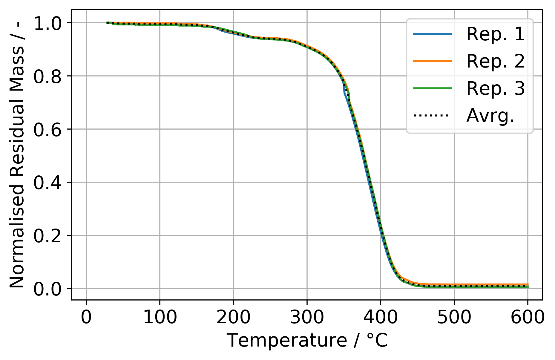
The focus of the micro-scale setups is to determine the temperature-dependent material decomposition reactions (pyrolysis). The experimental data, that is used as target during the parameter estimation, is taken from the open-access MaCFP git repository [7]. Two data sets are used in two different IMP setups. First, the normalised residual mass data recorded by a TGA with a heating rate of 10 K/min and heat release rate data recorded by an MCC with a heating rate of 60 K/min. Both are provided by the National Institute of Standards and Technology (NIST). Secondly, normalised residual mass data by a TGA from Sandia National Laboratories (Sandia), recorded at a higher heating rate of 50 K/min. This is used in an effort to get close to matching heating rates for TGA and MCC. As of writing, no 60 K/min TGA data set or MCC experiments with different heating rates matching the existing TGA data are available from the MaCFP repository. The TGA experiments by NIST were conducted in nitrogen atmosphere. For the MCC experiments the pyrolysis chamber was fed with nitrogen and oxygen was mixed into the effluents before entering the combustion chamber. The TGA experiments by Sandia were conducted in argon atmosphere.

All the experimental data series are averaged within each group, to be used as target during the IMP, see figure 1. The residual mass data is normalised to get the normalised residual sample mass over temperature, and the final residue amount is determined (figure LABEL:fig:TGA_exp_NIST). The amount of residue produced is very small, about one percent of the starting sample mass. This value is used directly as residue production for each decomposition reaction in FDS (NU_MATL). From the processed heat release rate data the average effective heat of combustion is determined.

Two different IMP setups are designed, summarised in table 2. They assess each parameter sets performance in two different simulation setups simultaneously. With this two experiment setups with different heating rates can be taken into account. The first micro-scale IMP setup uses the normalised residual mass at a heating rate of 10 K/min (TGA, NIST) and the heat release rate at 60 K/min (MCC, NIST). The second micro-scale IMP setup uses the normalised residual mass at a heating rate of 50 K/min (TGA, Sandia) and the heat release rate at 60 K/min (MCC, NIST). Thus, the first IMP setup covers a relatively large difference in the heating rate. The second setup aims to provide a heating rate in the TGA that closer matches the conditions during the MCC experiment, within the available data from MaCFP.

Table 2: Overview over the different micro-scale IMP setups, with two simultaneous simulations.

IMP Setup	IMP Target Details
	Simulation 1	Simulation 2
MCCTGA_01	normalised residual mass at 10 K/min (TGA)	heat release rate at 60 K/min (MCC)
MCCTGA_02	normalised residual mass at 50 K/min (TGA)	heat release rate at 60 K/min (MCC)

Table 3: Overview over the parameters of the pyrolysis scheme that are adjusted in the micro-scale IMP step.

Component	Parameter
PMMA 1 to 8	Reference temperature
	Pyrolysis range
	Heat of reaction
	Mass fraction
Fuel mixture	Carbon dioxide mass fraction
	Ethylene mass fraction
	Methane mass fraction

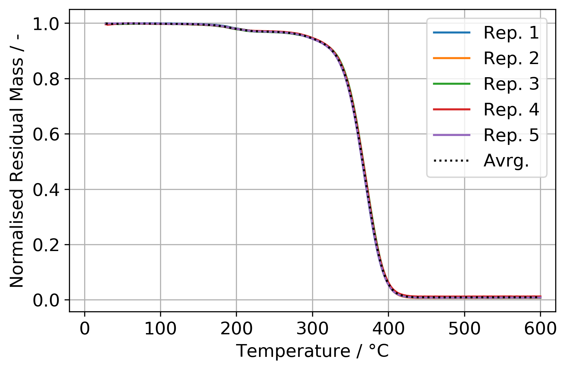
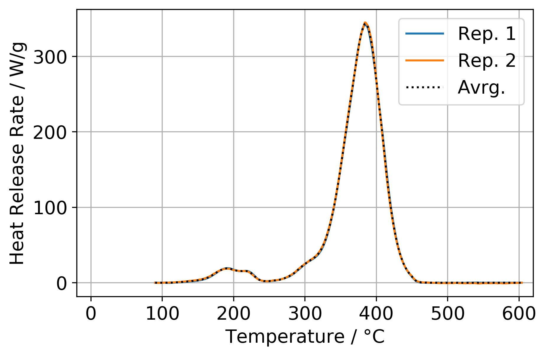
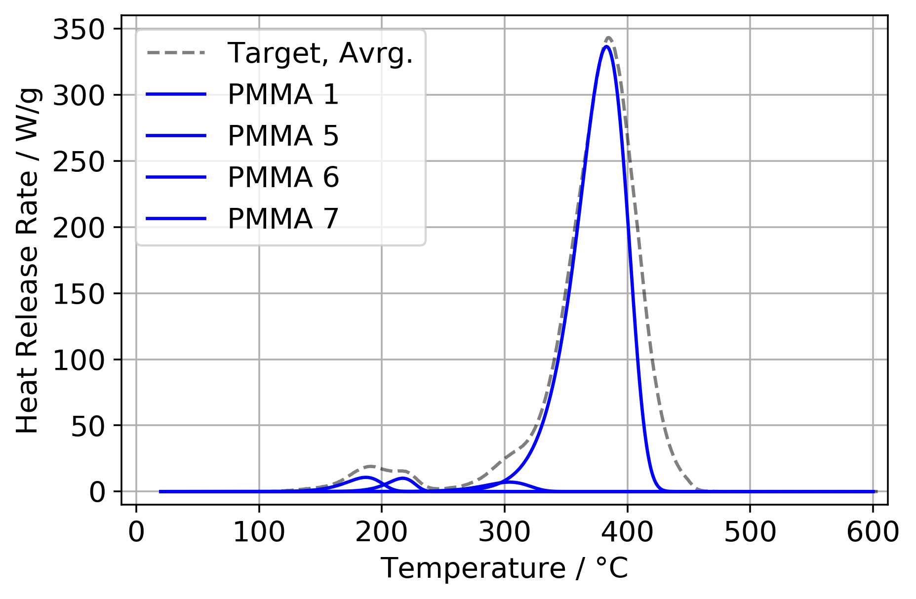
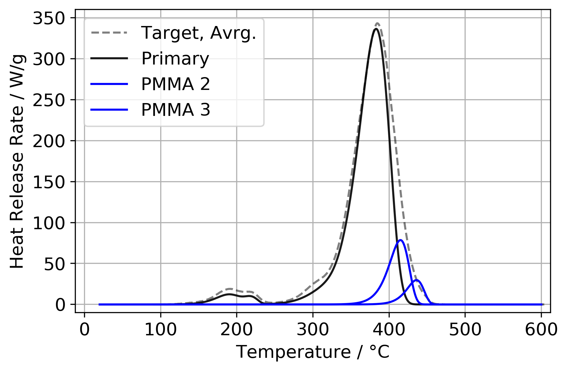
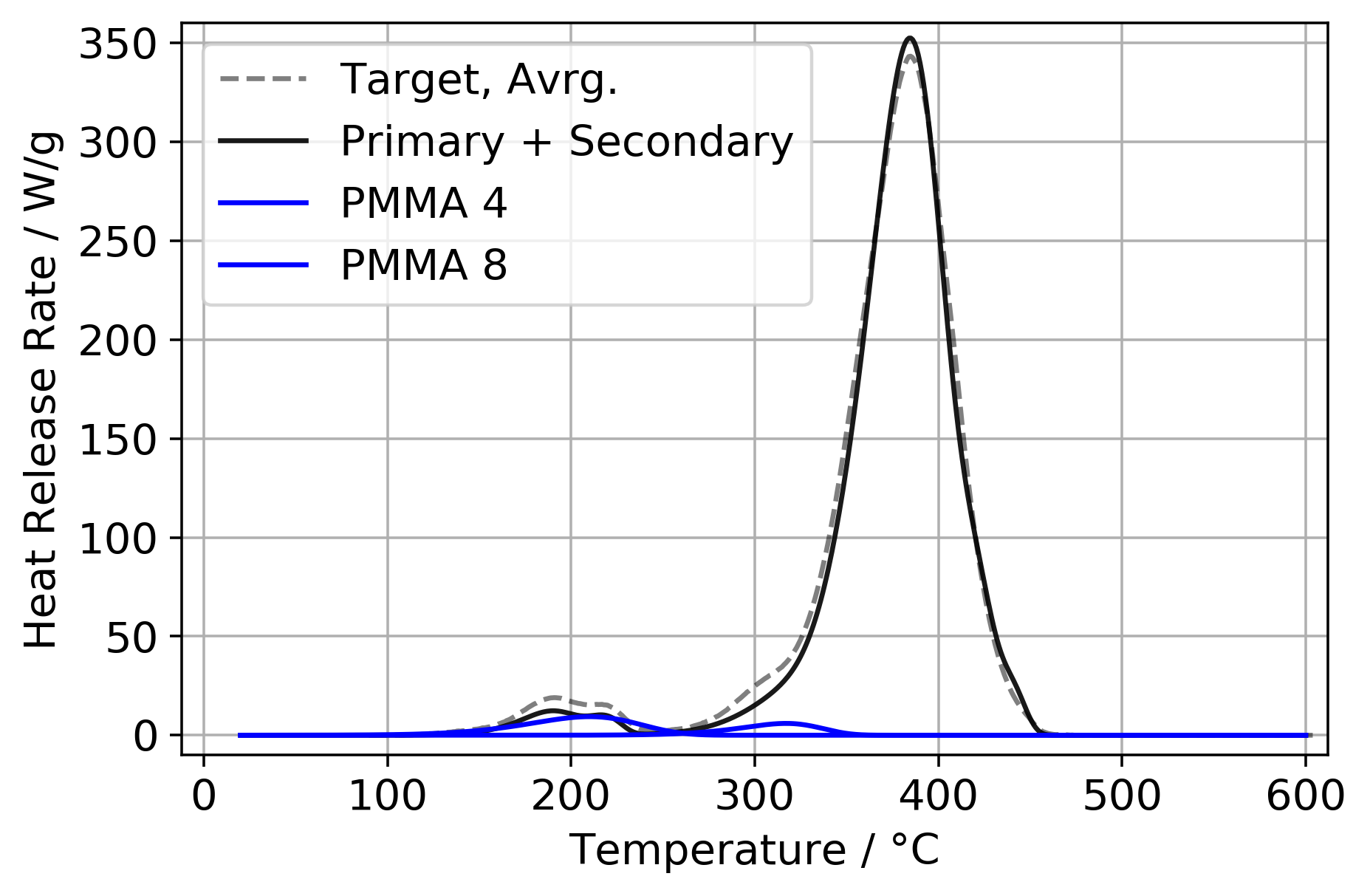
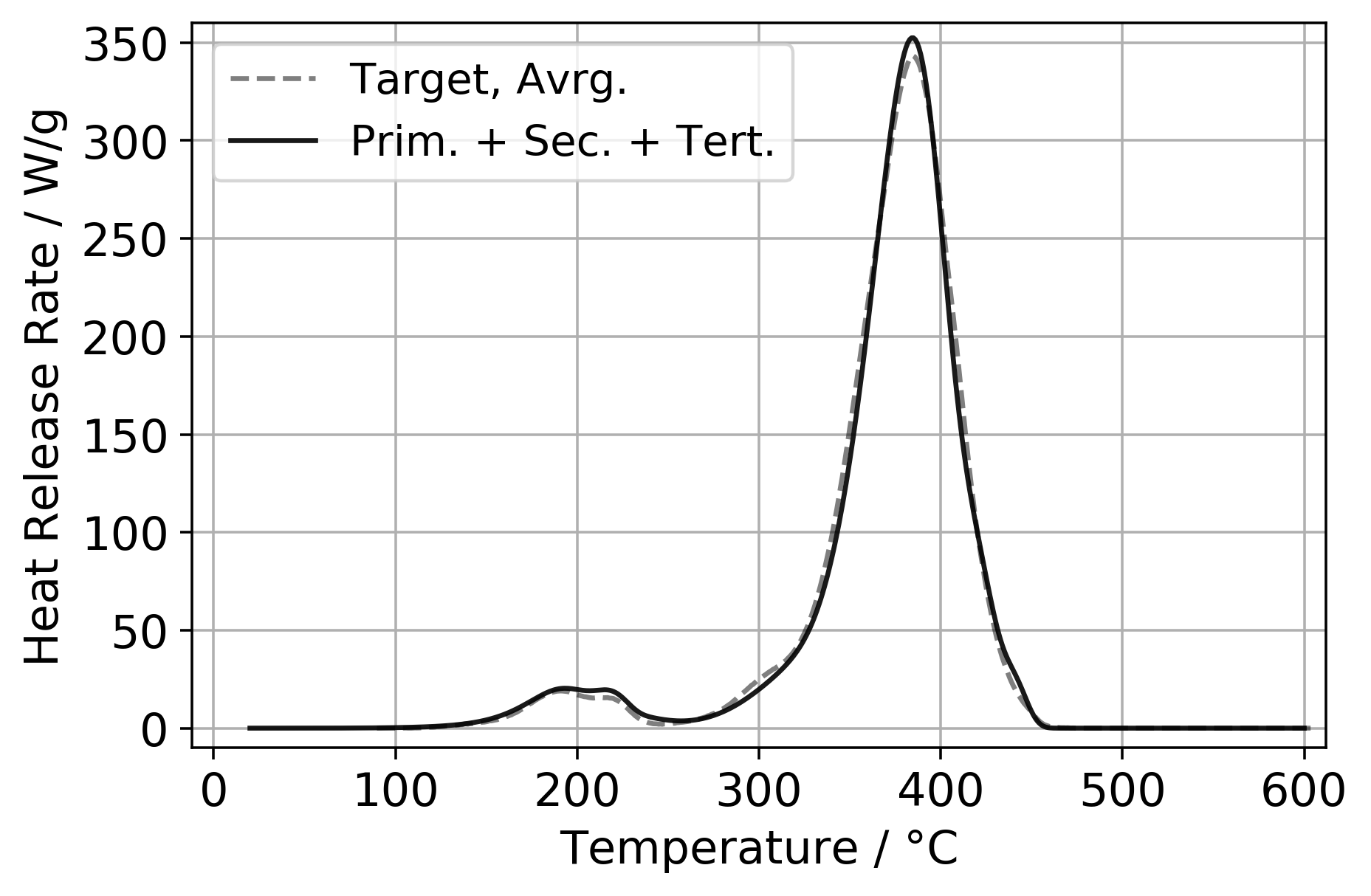
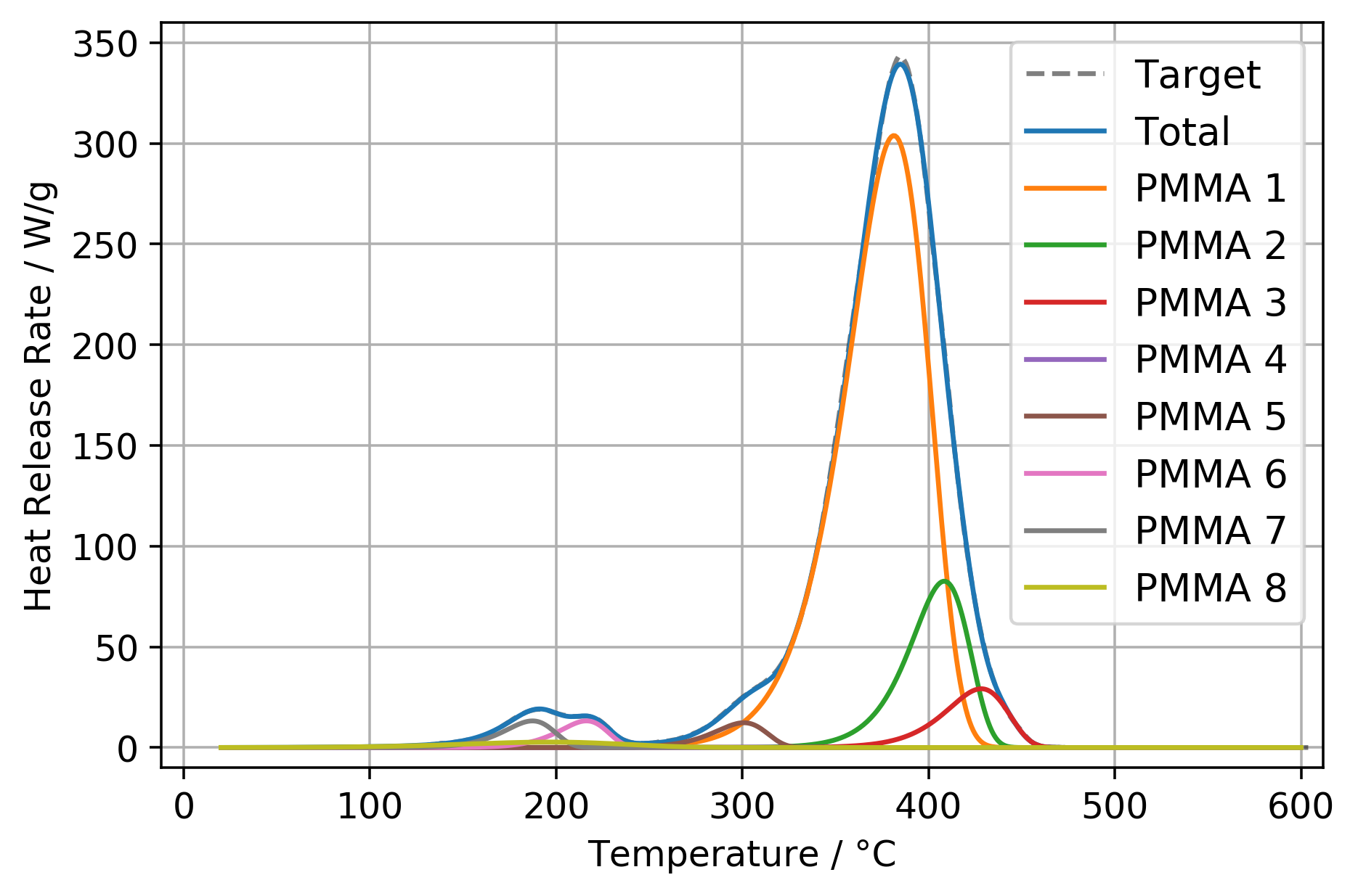
Multiple parallel pyrolysis reactions are used to roughly approximate the experiment data. The goal is to use as few reactions as possible, yet approximate the experiment response to a high precision. The reactions are manually positioned, by defining the reference values by trail-and-error. The parameters of these reactions form the first guess. The positioning process is conducted as follows. Individual decomposition reactions are identified from a plot of the MCC heat release rate experiment data, see figure LABEL:fig:MCC_exp_NIST. Four peaks can be visually identified at about 187 °C, 217 °C, 304 °C and 383 °C, see figure LABEL:fig:DecompositionScheme01. They form the primary set of decomposition reactions. A secondary set, figure LABEL:fig:DecompositionScheme02, is used to capture the decay of the largest reaction peak. They are located at 415 °C and 436 °C. This is necessary, because to skew the peak, reaction orders larger than unity would be needed. The skewing behaviour needs therefore be reproduced by superposition of multiple reactions. Finally, a set of tertiary reactions is defined at about 210 °C and 317 °C, see figure LABEL:fig:DecompositionScheme03. They are used to provide the optimiser with some flexibility to capture the reaction rate development. All these reaction sets combined form the initial guess of the decomposition scheme for the inverse modelling, see figure LABEL:fig:DecompositionScheme04. Thus, these pyrolysis reactions are not necessarily directly chemical/physical in nature, but needed for the model. In total, eight decomposition reactions are defined, labelled "PMMA 1" to "PMMA 8". The fine-tuning of the parameters of these reactions, using an IMP, concludes the first step of the procedure.

The argument could be made, that eight pyrolysis reactions are too many. One might be able to exclude the tertiary reactions. However, the algorithm is not able to add more reactions if needed, but can only adjust predefined parameters. Since it is unclear in the beginning how many reactions are necessary more decomposition reactions are added to provide the algorithm with some flexibility.

The above decomposition scheme is implemented as follows. An FDS functionality (TGA_ANALYSIS) is used to evaluate an extremely simplified micro-scale simulation setup. It linearly increases the temperature of a mass sample and tracks the pyrolysis. The pyrolysis is simulated by employing Arrhenius equations for multiple decomposition reactions. The Arrhenius model is used as provided with FDS.

FDS offers some convenience functionalities where the Arrhenius parameters (pre-exponential factor A, activation energy E) can be deduced from the peak temperature of the decomposition reaction rate and the width of the peak. These reference values are entered by the user as REFERENCE_TEMPERATURE and PYROLYSIS_RANGE. In this procedure, the reaction order is assumed to be unity. The heating rate of the experiment that serves as starting point needs to be provided to FDS as well.

In FDS, the decomposition reactions are associated with the material definitions (MATL). Thus, the material definitions provide two functions: 1) define the thermophysical properties of a material and 2) define its pyrolysis reaction. While the pyrolysis reaction parameters are here determined during the first IMP step, the thermophysical parameters are determined in the second IMP step, see section 4. The different materials (MATL) are realised into a sample, by combining them into a boundary condition (SURF). In the case here, the PMMA sample needs to combine eight different material definitions to account for the decomposition reactions. All the pyrolysis reactions are directly converting the PMMA material into a gas mixture and an inert residue, see section 2.3. The individual contributions of the reactions are controlled by mass fractions of the materials, set in the PMMA sample definition. This means that each reaction has access to a predefined amount of sample mass. Furthermore, each material definition is assigned a heat of reaction (HOR), which is also determined during this first IMP step. In total, four parameters describe a single reaction and are determined with the IMP: the two reference values, the sample mass fraction per reaction and the respective HOR, see table 3. The overall fitness value is a combination of the performance in the MCC and in the TGA simulations.

The thermophysical parameters are identical for all eight material definitions, to realise a homogeneous PMMA sample, and are determined in the second IMP step, see section 4.

3.2 Results

Two IMP runs with different simulation setups have been conducted (table 2). Both converge to their best fitness values within about 40 generations, see figure 3. The simulation responses of the best parameter sets for both IMPs are compared against their TGA target data for both heating rates, see figure 4. The "(IMP)" marks which IMP used the respective target. The mass loss for a heating rate of 10 K/min happens at lower temperatures in the simulation for both IMPs, with MCCTGA_01 being slightly closer to its target (figure LABEL:fig:TGA_10K_best_IMP). For a heating rate of 50 K/min, both yield a very similar response (figure LABEL:fig:TGA_50K_best_IMP).

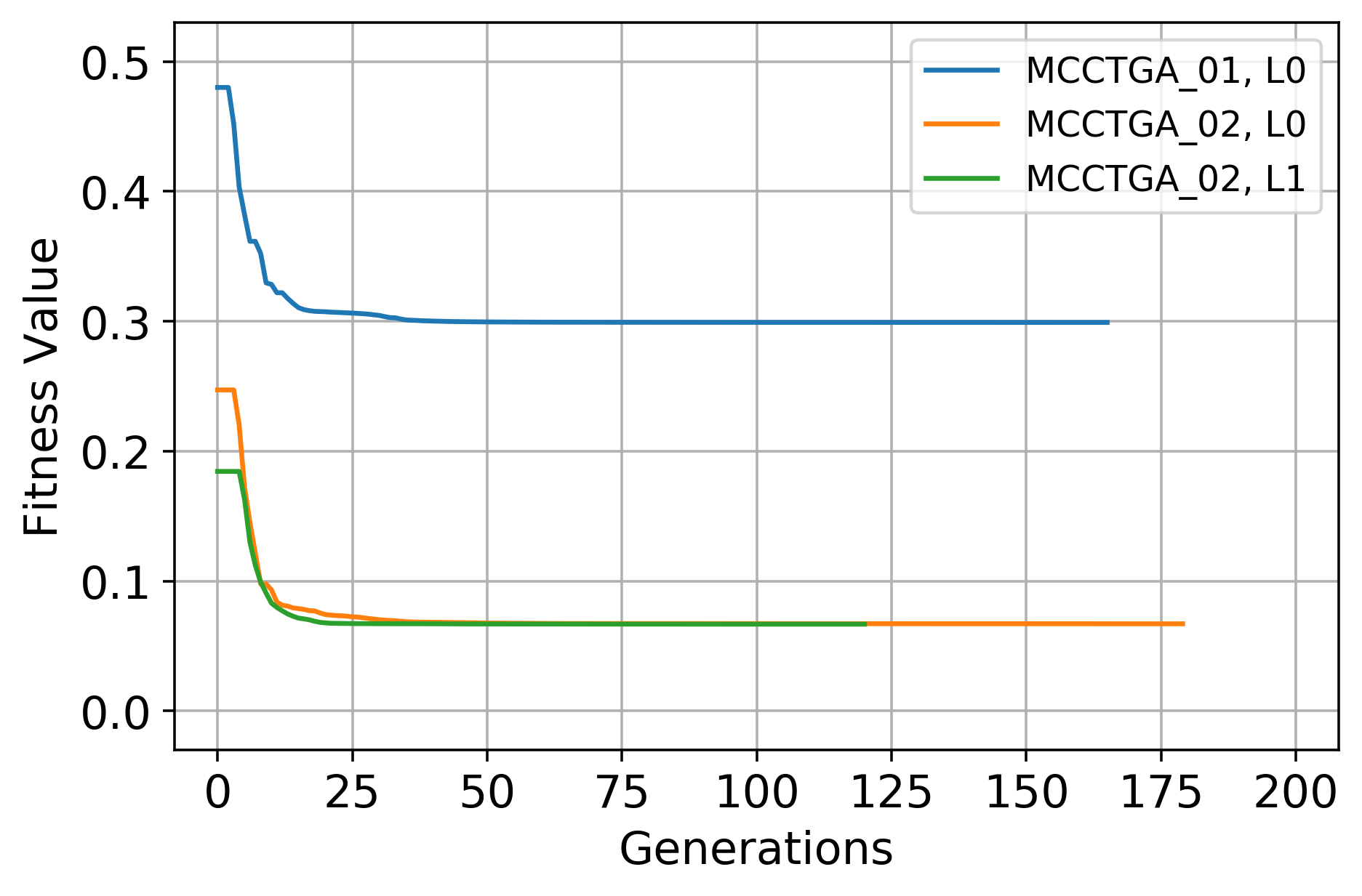
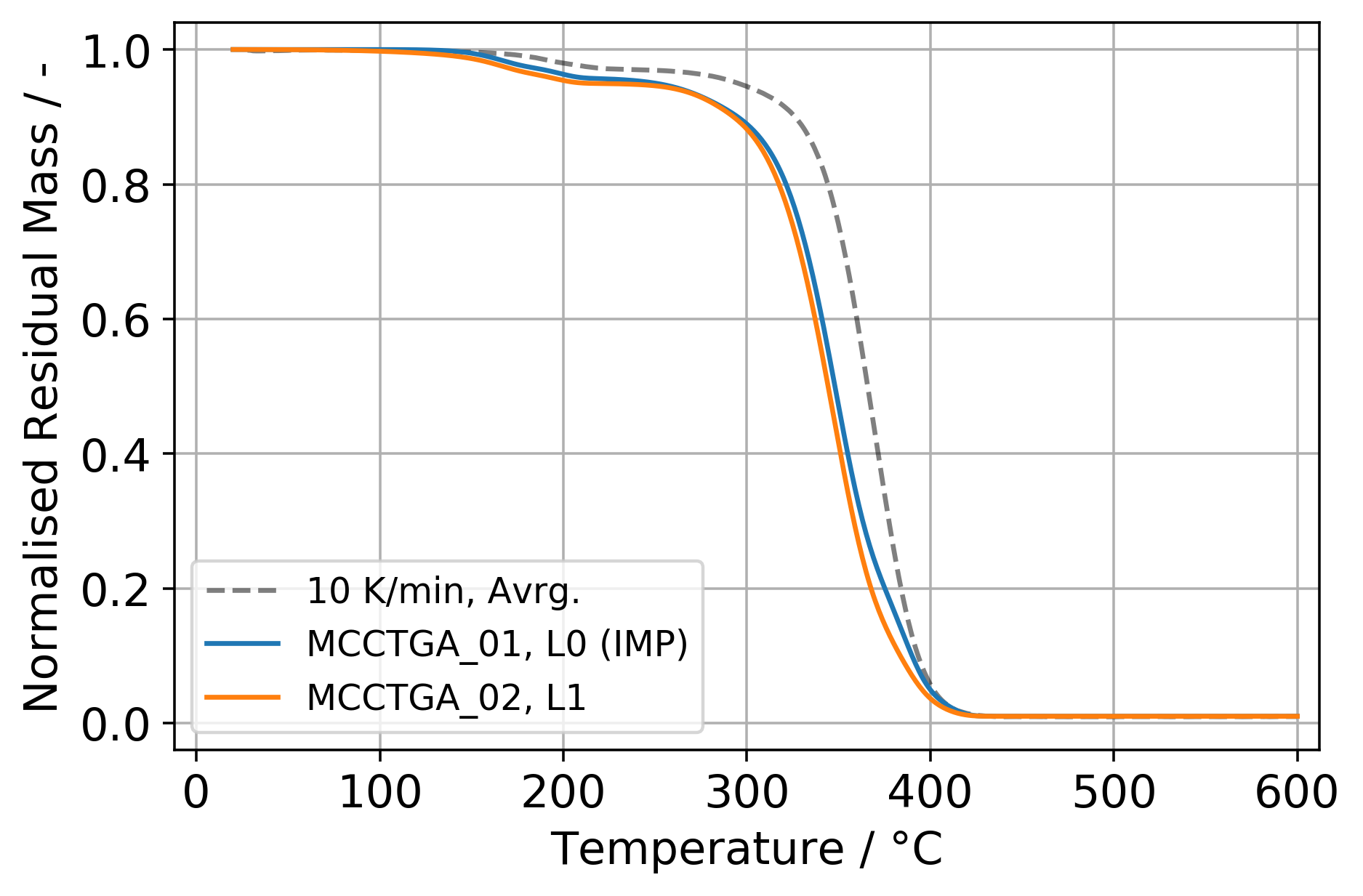
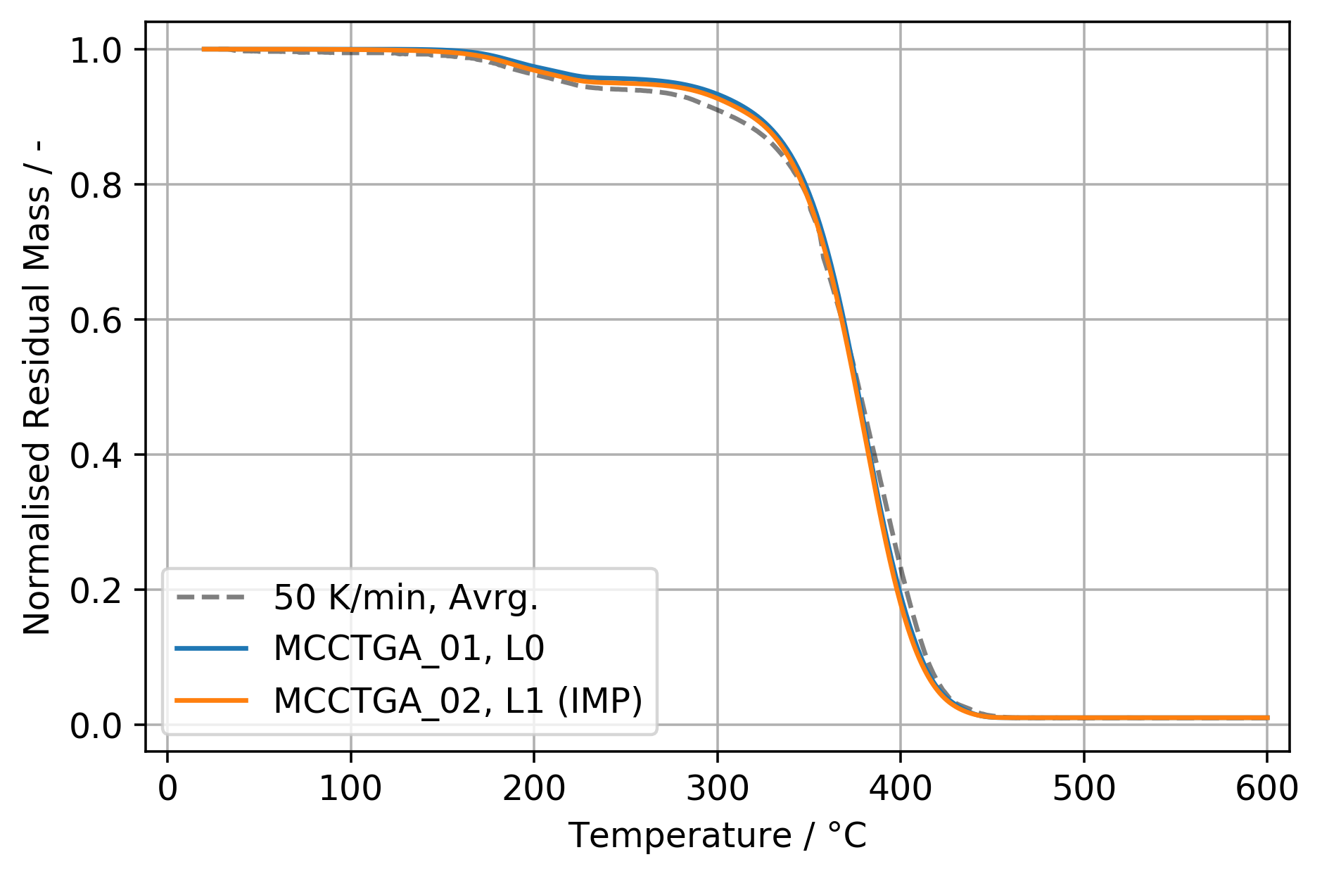
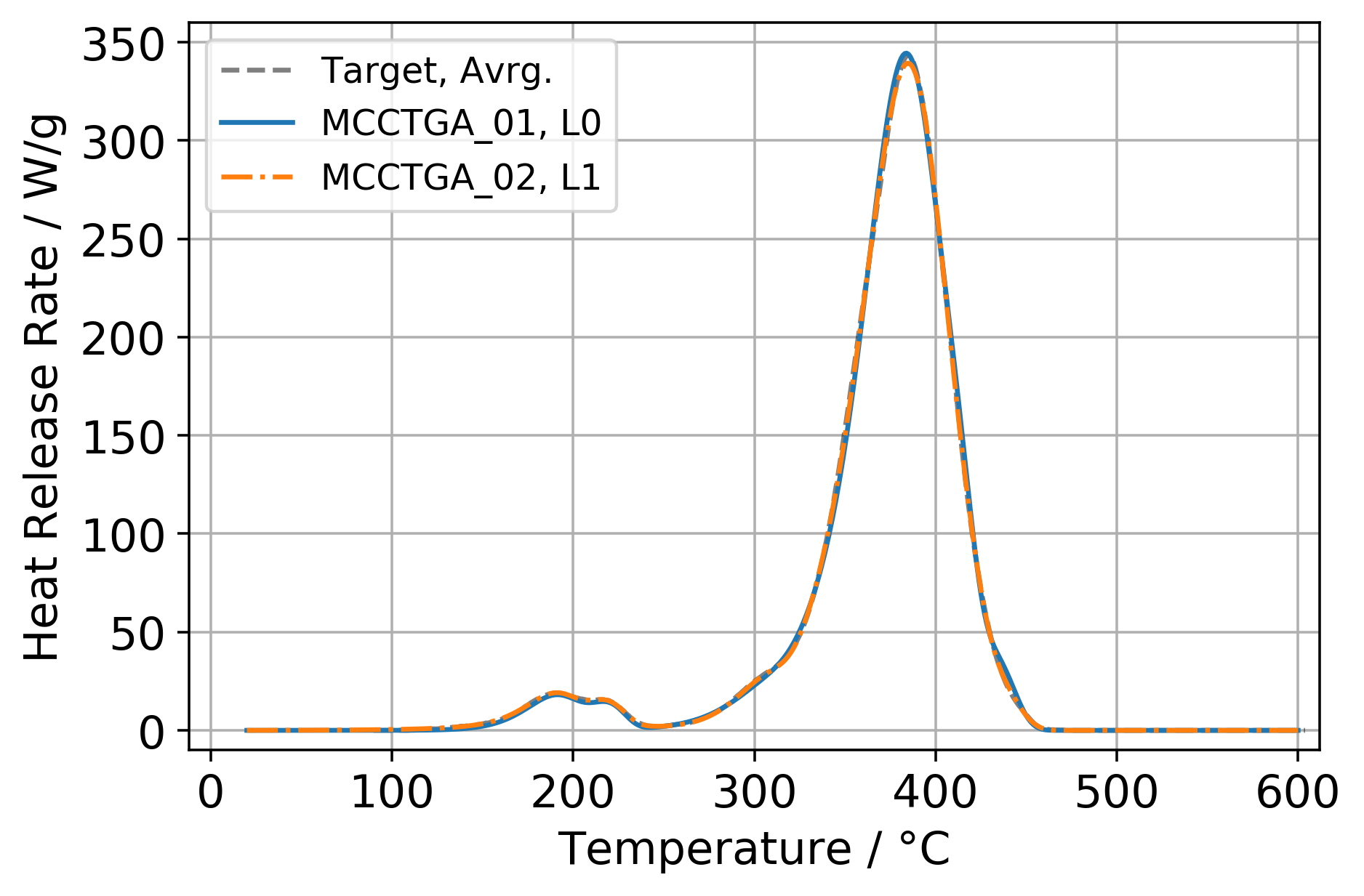
Figure LABEL:fig:MCCTGA02_L1_IndivReac_locations shows the eight predefined decomposition reactions, after being fine tuned through the IMP. The tertiary reactions "PMMA 4" and "PMMA 8" provide significantly lower contributions compared to the other reactions (figure LABEL:fig:MCCTGA02_L1_IndivReac_contribution).

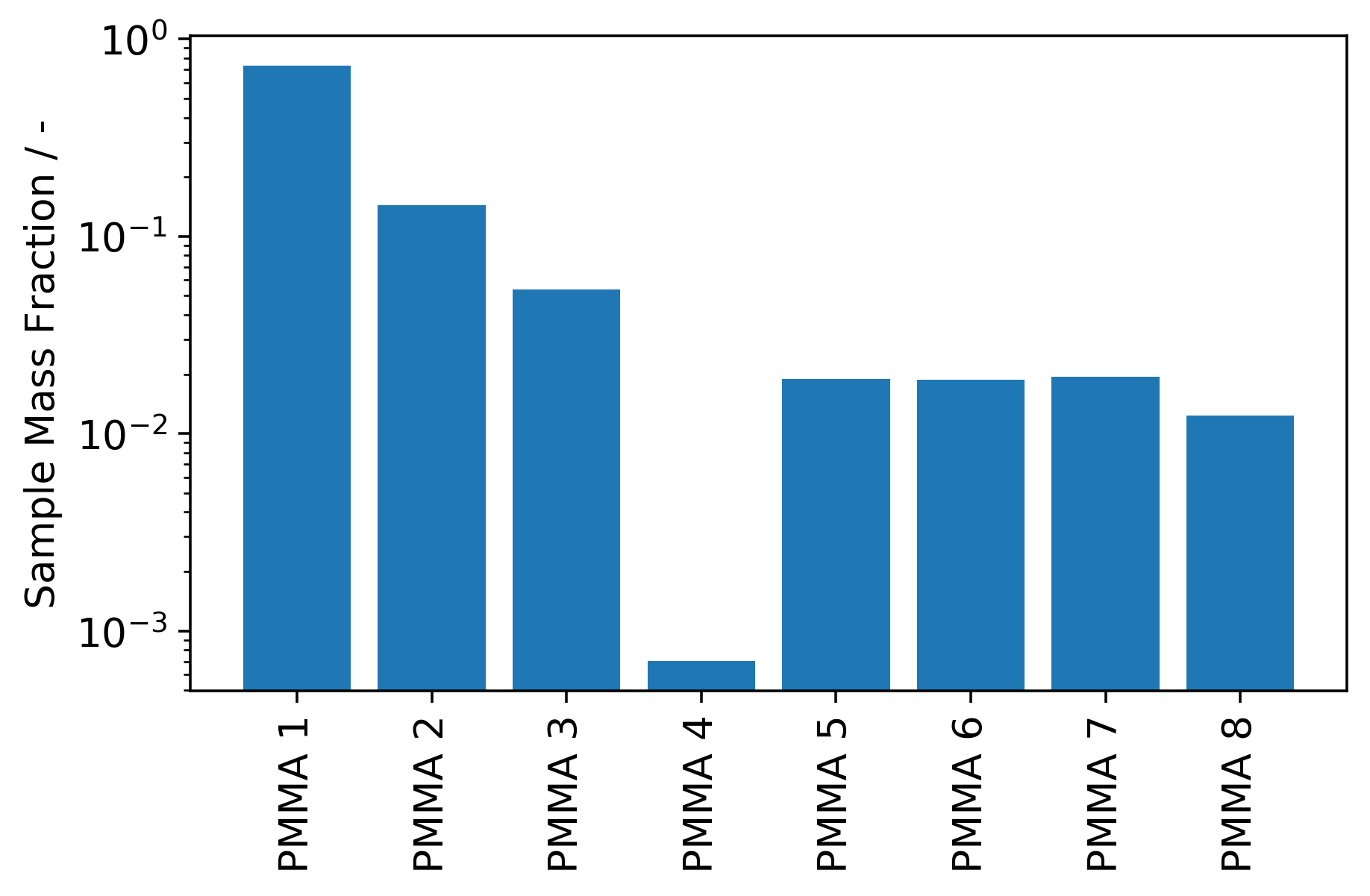
Due to its better fitness value, focus is shifted to MCCTGA_02 and no further sampling limit adjustment is conducted for MCCTGA_01. MCCTGA_02 is used in the following cone calorimeter simulations.

3.3 Discussion

Both IMP setups are able to reproduce the MCC data well (figure 5). The TGA data for a heating rate of 50 K/min is better reproduced than for 10 K/min (figure 4). The deviation between simulation and experiment for 50 K/min is attributed to the non-linear heating rate in the experiment, see figure LABEL:fig:Apdx_MicroScale_HeatingRates_Sandia50K. Larger differences between experiment and simulation are observable for a heating rate of 10 K/min. Here, MCCTGA_01 gets slightly closer to its target. Otherwise, the results are similar, yet happen at lower sample temperatures compared to the experiment. With the lower heating rate in the TGA (MCCTGA_01) the algorithm is not able to find a parameter set suitable for both conditions, i.e. 10 K/min in the TGA and 60 K/min in the MCC. It comes as some surprise that the IMP favours the MCC and does not position the fit somewhere in between both targets. Some bias may have been built into the setup, by manually positioning the first guess reactions based on the MCC data, or by the chosen cost function.

Possibly, some aspects of the apparatus are not captured well enough in the highly simplified micro-scale model. We know, from private communication with Karen De Lannoye, that the design of the TGA apparatus has an observable impact on the results [43]. Ding et al. reported an observable shift of reaction rate peaks to lower temperatures in MCC experiments when compared to TGA data at the same heating rate [2]. They adjusted the heat release data from the MCC by shifting it to higher temperatures, about 4 K to 20 K. At the point of writing, in the MaCFP repository no data series for both experiments at the same heating rate are reported, which makes a similar assessment here difficult. The shift seems also to depend on the material. More experiment data is necessary for this comparison.

The divergence could also be related to the released gas mixture, which in this contribution assumes an average heat of combustion over the course of the experiment. It is argued [15], that the first peak at about 187 °C (figure LABEL:fig:MCC_exp_NIST) could be attributed to residual solvent within the polymer. Furthermore, radically polymerised PMMA is somewhat unstable and starts decomposition at about 220 °C, due to unsaturated end groups [14]. Even though the primary decomposition products of PMMA are MMA and carbon dioxide, the MMA is not directly involved in the gas phase combustion [14]. Some major compounds involved in the combustion of PMMA are methane, methanol, formaldehyde and acetylene, with ethylene being involved during the acetylene combustion. As an example, for pure compounds the heats of combustion are tabulated in the literature [45] with 50.0 MJ/kg for methane, 50.4 MJ/kg for ethylene, 19.8 MJ/kg for methanol and 24.2 MJ/kg for PMMA. If these compounds are produced at different, temperature-dependent rates, they could lead to a variable effective heat of combustion over the course of the experiment. In the work presented here, a mixture of methane, ethylene and carbon dioxide is released during the PMMA pyrolysis. The individual fractions are adjusted during the IMP. However, that leads to a constant average heat of combustion of the PMMA pyrolysis products throughout the simulation. A model allowing for a variable HOC could be an additional degree of freedom in the IMP to match the MCC and TGA data. Fixing this mixture over all reactions could be too rigid. In future work individual mixtures will be investigated. The difference for the TGA test at 10 K/min, see figure 4, could be a manifestation of this rigidness, as low and high heating rates need to be reproduced simultaneously. A possible solution would be to use multiple gas mixtures. In an effort to reduce complexity downstream, i.e. definition of multiple chemical reactions and solving more transport equations, the mixture could be generated on-the-fly by releasing a single species per reaction. It might also be sufficient to mix only methane and carbon dioxide. Each decomposition reaction in figure 6 could be doubled. One would release methane and the other carbon dioxide, the mixture would then be controlled from the mass fraction in the surface definition. This strategy is to be investigated in future work.

Here, no IMP target is provided to explicitly match the heats of reaction for the individual decomposition reactions. This could be accomplished by using experiment data from differential scanning calorimetry (DSC). Alonso et al. [5] used TGA and DSC data as targets in their IMP setup, changing the contribution of each to the overall fitness assessment. With this, the target of higher importance is reproduced better to the detriment of the other. The employed decomposition scheme uses two consecutive decomposition reactions forming an intermediate material and a residue. A parallel decomposition scheme, as is proposed here, could be able to capture more gradual changes in the heats of reaction across the temperature range of the experiment. This could improve the overall performance of the parameter sets generated here and should be investigated in future work.

The proposed approach using gas mixtures allows to model more sophisticated technical materials. Specifically, the behaviour of fire retardant materials could be reproduced. Non-combustible gas could be released early on, which cannot be captured with a single surrogate fuel. This makes it necessary to take MCC and TGA data into account simultaneously. This could even be expanded further, by adjusting which reaction contributes most to the production of the residue. Also considering different residues, for example for intumescent materials.

Arguably, the goal to use as little decomposition reactions as possible is not achieved. Looking at figure 6, PMMA 4 ( $0.07\%$ ) could be removed, possibly also PMMA 8 ( $1.23\%$ ) – even tough it is not too far off of PMMA 6 ( $1.88\%$ ). It should be noted that there is an error in the definition of the pyrolysis reaction input for PMMA 4. Its heating rate is set to 80 K/min instead of the desired 60 K/min. Since the contribution of PMMA 4 is negligible, it is regarded inconsequential here. This is confirmed with a corrected IMP, see data repository (MCCTGA_2b) [28], which virtually yields the same result.

4 Bench-Scale Setup — Thermophysical Material Parameters

4.1 Methods

The second IMP step is used to determine the thermophysical parameters of the PMMA material model. They are determined in the bench-scale from cone calorimeter experiments. The cone calorimeter experiment data, provided by Aalto University, is taken from MaCFP [7]. According to the reported information, the experiments have been conducted at a radiative heat flux of 65 kW/m², without a retainer frame. Square samples of cast black PMMA, with an edge length of 10 cm and a thickness of 0.6 cm, were used. These samples were placed onto the sample holder, atop a layer of insulating ceramic wool, with a thickness of about 2.0 cm.

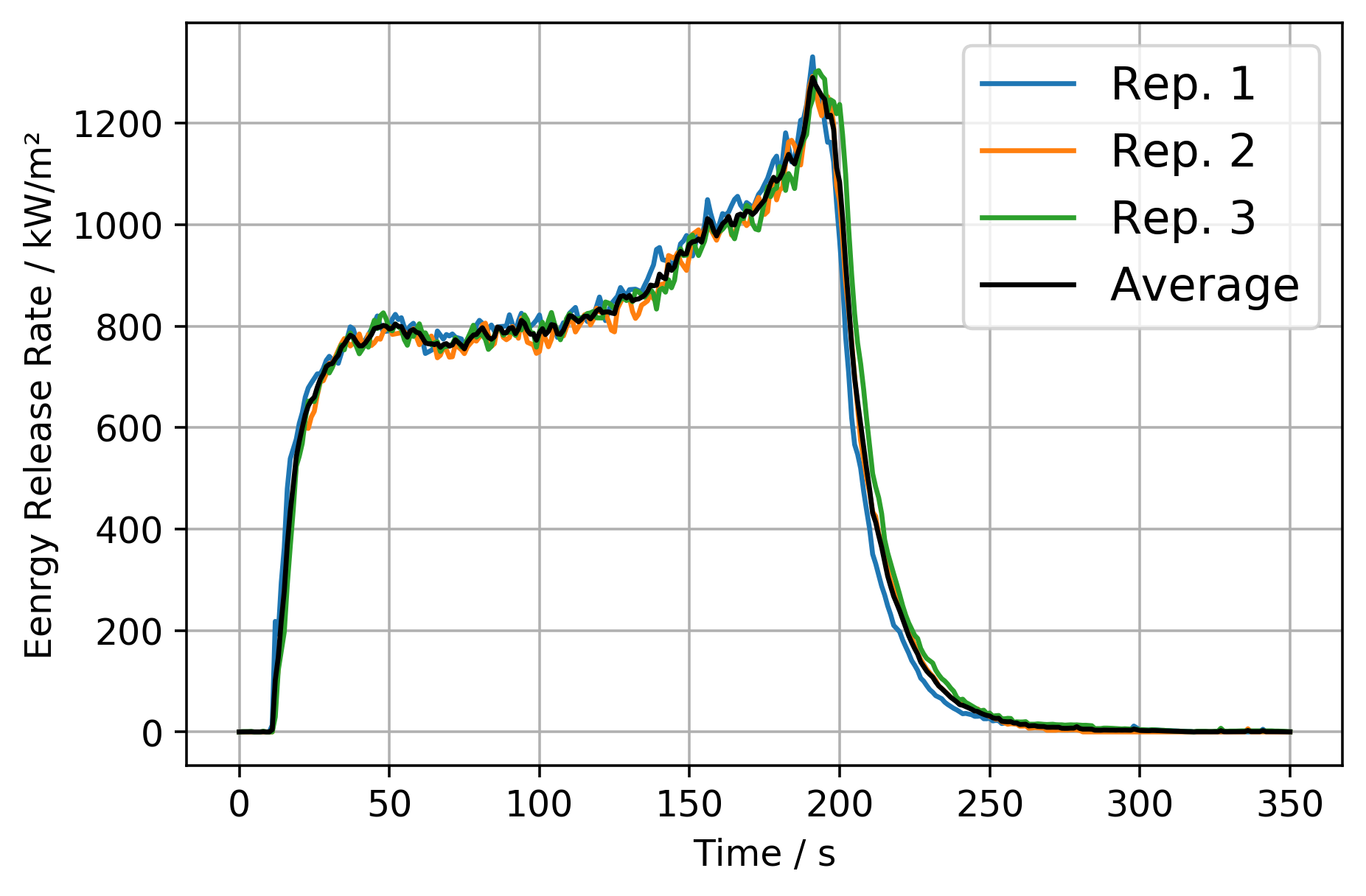
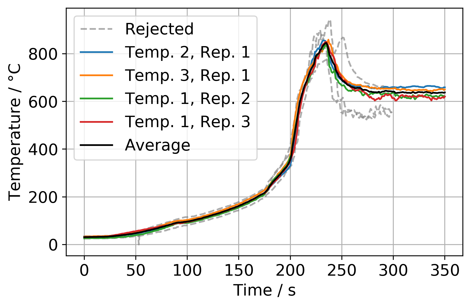
As target data for this inverse modelling step the heat release rate and the back face temperature of the sample are chosen. They are processed similarly as described in section 3.1. The experiments show good repeatability, as demonstrated by the heat release rate in figure LABEL:fig:ConeExpAalto_err. Thermocouples have been placed between the insulation layer and PMMA sample to record the back face temperature of the sample. Temperatures have been recorded at the centre of the back face (Temp_1) and at two opposite locations with a radial distance of 1.5 cm around the face centre (Temp_2/3). Regardless of their location, most thermocouples show very similar temperature development, see figure LABEL:fig:ConeExpAalto_temp. Few diverge and are rejected here, due to assumed sample deformation, see discussion in section 4.3.

The simplified cone calorimeter simulation setup, as outlined below, is designed to enable gas phase combustion, while keeping the IMP in a manageable time frame (table 1). It allows the formation of a flame, which is based on the combustible mass released from the sample. This in contrast to an approach without the gas phase, where the flame heat flux would need to be prescribed and would effectively define a static imaginary flame with no connection to the gas phase model. Simulation setups neglecting the gas phase combustion altogether impact the parameter estimation. In principle, surrogate fuels could be changed between setups, because FDS would maintain the heat release by using the heat of combustion value, set in the material definition (MATL), see section 2.4. However, the heat feedback from the flame is important to take into account. For example, different surrogate fuels can have different radiative fractions (see table 16.1 in [23]). The influence of the flame, formed from the chosen surrogate, will impact the determined material parameter set. In the presented work, care is taken to use the same surrogate fuel throughout all scales, to not introduce errors when changing between setups.

During the IMP, the cone calorimeter apparatus is simulated in a simplified way. The simulation mode in FDS is set to LES (Large Eddy Simulation) to facilitate the transfer to the real-scale setup, by maintaining model consistency across scales. The computational domain is a single mesh and computed by a single computing core. The sample is assumed to be a square with an edge length of 10 cm. The domain extents 30 cm in the x- and y-directions, with the sample centred. From the top of the sample, the domain extents 60 cm in the positive and two cells in the negative z-direction. Throughout this document, the fluid mesh resolutions are referred to by the number of fluid cells dividing a sample top face edge. For example, consider that each edge is divided by 3, thus $3\times 3$ cells cover the sample top surface. This is referred to as "C3". It results in an edge length for the individual fluid cells of 3.33 cm. Consequently, for C5 the cell edge length is 2.0 cm and $5\times 5$ cells are covering the sample surface. The primary simulation setup for the IMP uses the "C3" resolution. Figure 24 in the appendix provides a graphical overview over the domain layouts.

The sample holder assembly is reproduced as a boundary condition (SURF) with two layers. The top layer is associated with the PMMA material, the bottom layer with the insulation material. In an effort to separate the sample from the insulation and holder, the values of the insulation material are adjustable during the IMP. This leads to an artificial material that can compensate some influence of the boundary conditions in the experiments. It is called "backing" throughout this text.

The separation between sample and backing is to be achieved by using the back face temperature as IMP target. Regardless of their recording location in the experiment, the temperatures are very close to each other (figure LABEL:fig:ConeExpAalto_temp). With "C3" being the primary resolution, all temperature locations from the experiment fall into the face area of the single centre fluid cell in the simulation. Thus, in the simulation it is not possible to distinguish between these locations.

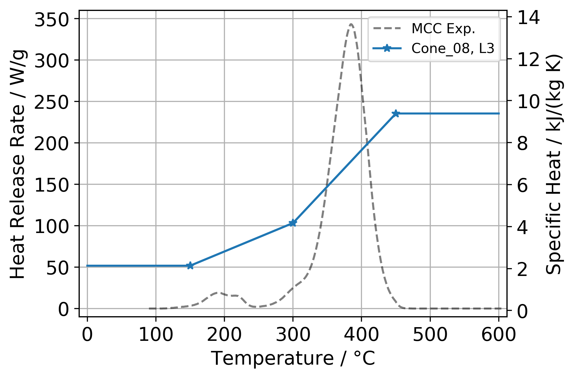
To study the impact of different IMP setups, a couple variations of IMP targets and simulation setups are used. They vary with respect to the temperature-dependent specific heat and thermal conductivity definitions, IMP targets, as well as fluid cell sizes. These IMP variations are built on a base case, labelled "Cone_01" (table 4). For it, the PMMA density ( $\rho$ ) is computed to about 1201.72 kg/m³, based on the reported sample mass and dimensions. The remaining thermophysical and optical parameters are: emissivity, absorption coefficient, refractive index, specific heat capacity ( $c$ ) and thermal conductivity ( $k$ ). They are solely determined during the IMP. A summary of the adjusted parameters for the base case is provided in table 5. Their initial sampling ranges are guessed and changed with successive limit adjustments, see section 2.2. Parameters for the pyrolysis and combustion are taken from the micro-scale IMP (MCCTGA_02), see section 3.2. Thermal conductivity and specific heat for the sample material are represented as temperature dependent values (RAMP). The parameter values are adjusted during the IMP, while the temperature points are fixed. In Cone_01 and Cone_03 to 05 the three temperature points are arbitrarily chosen to be 150 °C, 480 °C and 800 °C. In Cone_06 and Cone_07 the temperature values are determined based on the significant temperature interval of the MCC measurement, see stars in figure 8. The chosen values are 150 °C, 300 °C and 450 °C to represent this interval. They are also used for Cone_08, but here the conductivity for PMMA and the backing material are in addition using the low temperature data reported by DBI/Lund from the MaCFP materials database [7].

In general, the backing material and the residue are treated as unknown. The density of the backing material is set to 65 kg/m³, taken of the insulation material from the Aalto contribution [7]. The density of the residue is chosen arbitrarily to be 2500 kg/m³. For backing and residue, their individual emissivity, thermal conductivity and specific heat are adjusted during the IMP. The respective sampling ranges are guessed. This is intended to provide some degrees of freedom, in an attempt to separate the sample behaviour from the boundary conditions of the experiment. The back face temperature is used as IMP target to achieve this separation. For one IMP setup (Cone_04) only the energy release is used as target to serve as comparison. With respect to fluid cell sizes, the default is C3. However, Cone_05 uses the C5 and Cone_07 the C2 setup. An overview of all investigated setups is outlined in table 4.

Table 4: Overview over the different simplified cone calorimeter IMP setups. PMMA density is 1201.72 kg/m³ for all cases.

IMP Setup	Details	Resolution	Target
Cone_01	Base case	C3 (3.3 cm)	HRR, Temperature
Cone_02	Temperatures for the specific heat and conductivity	C3 (3.3 cm)	HRR, Temperature
	RAMPs based on FDS parallel panel validation case
Cone_03	PMMA slab thickness set to 6.1 mm	C3 (3.3 cm)	HRR, Temperature
Cone_04	Base case	C3 (3.3 cm)	HRR
Cone_05	Base case	C5 (2.0 cm)	HRR, Temperature
Cone_06	Temperatures of conductivity and spec. heat RAMPs	C2 (3.3 cm)	HRR, Temperature
	based on MCC plot (figure 8)
Cone_07	Like Cone_06	C2 (5.0 cm)	HRR, Temperature
Cone_08	Like Cone_06, lower temperature data added to RAMPs	C3 (3.3 cm)	HRR, Temperature
	for conductivity of PMMA and insulation, from DBI [7]

Table 5: Overview over the parameters that are adjusted in the bench-scale IMP step, base case.

Material	Parameter
PMMA	Emissivity
	Absorption coefficient
	Refractive index
	Conductivity at 150 °C
	Conductivity at 480 °C
	Conductivity at 800 °C
	Specific heat at 150 °C
	Specific heat at 480 °C
	Specific heat at 800 °C
Residue	Emissivity
	Conductivity
	Specific heat
Backing	Emissivity
	Conductivity
	Specific heat

The PMMA sample and the insulation layer below it are defined as a layered boundary condition (SURF). The cell size for the solid phase is determined by FDS automatically, based on the density, thermal conductivity and specific heat capacity (thermal diffusivity: $k/(\rho c)$ ). By default the cell size changes across a layer thickness, providing the highest resolution towards the surfaces. For the PMMA layer the cell size is forced to be uniform (STRETCH_FACTOR=1). The resolution is further increased by a factor of 10 (CELL_SIZE_FACTOR=0.1). Since the thermal conductivity and specific heat capacity are adjusted during the inverse modelling, the solid cell size changes for any given PMMA material parameter set during the estimation process. The insulation layer uses the FDS default settings.

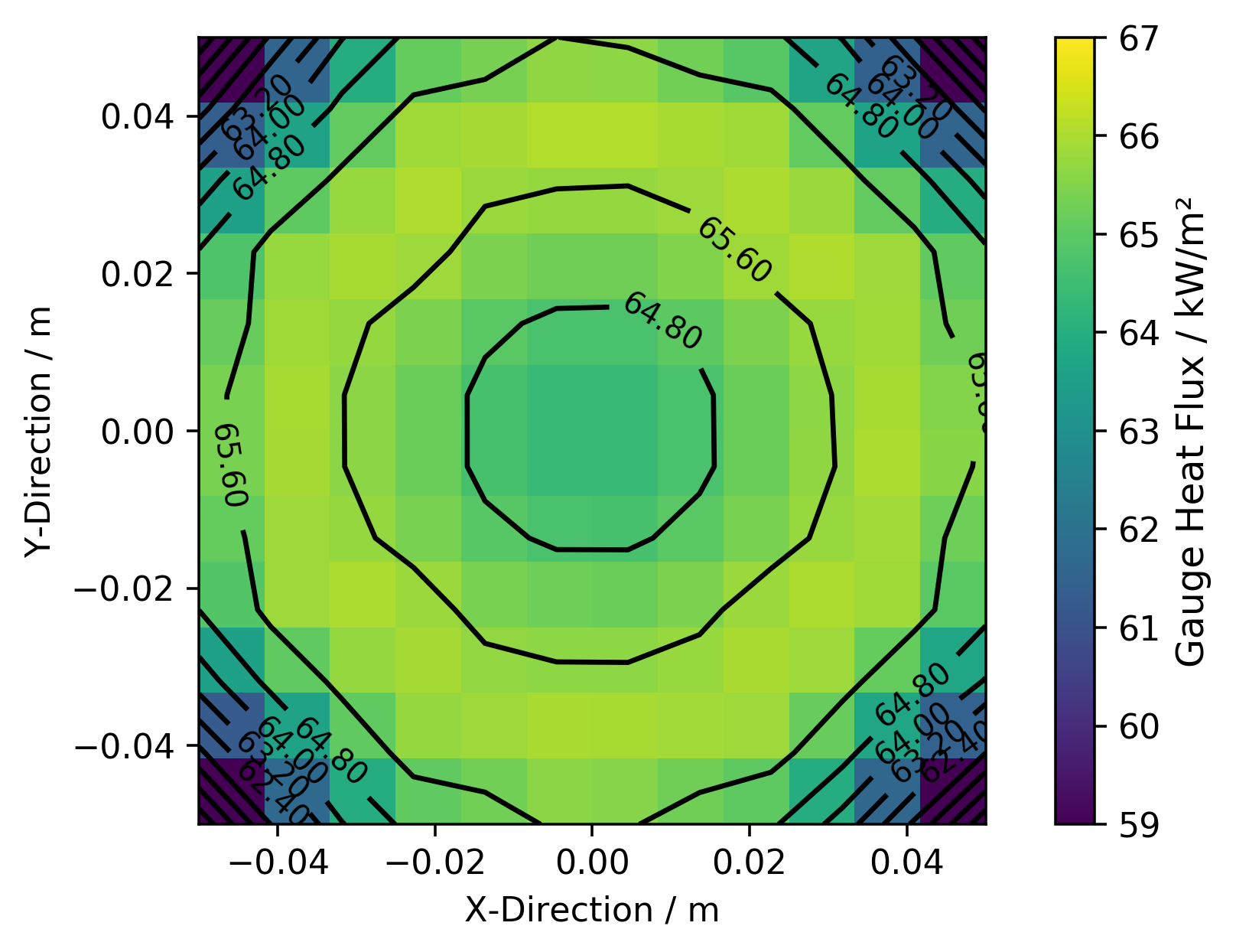
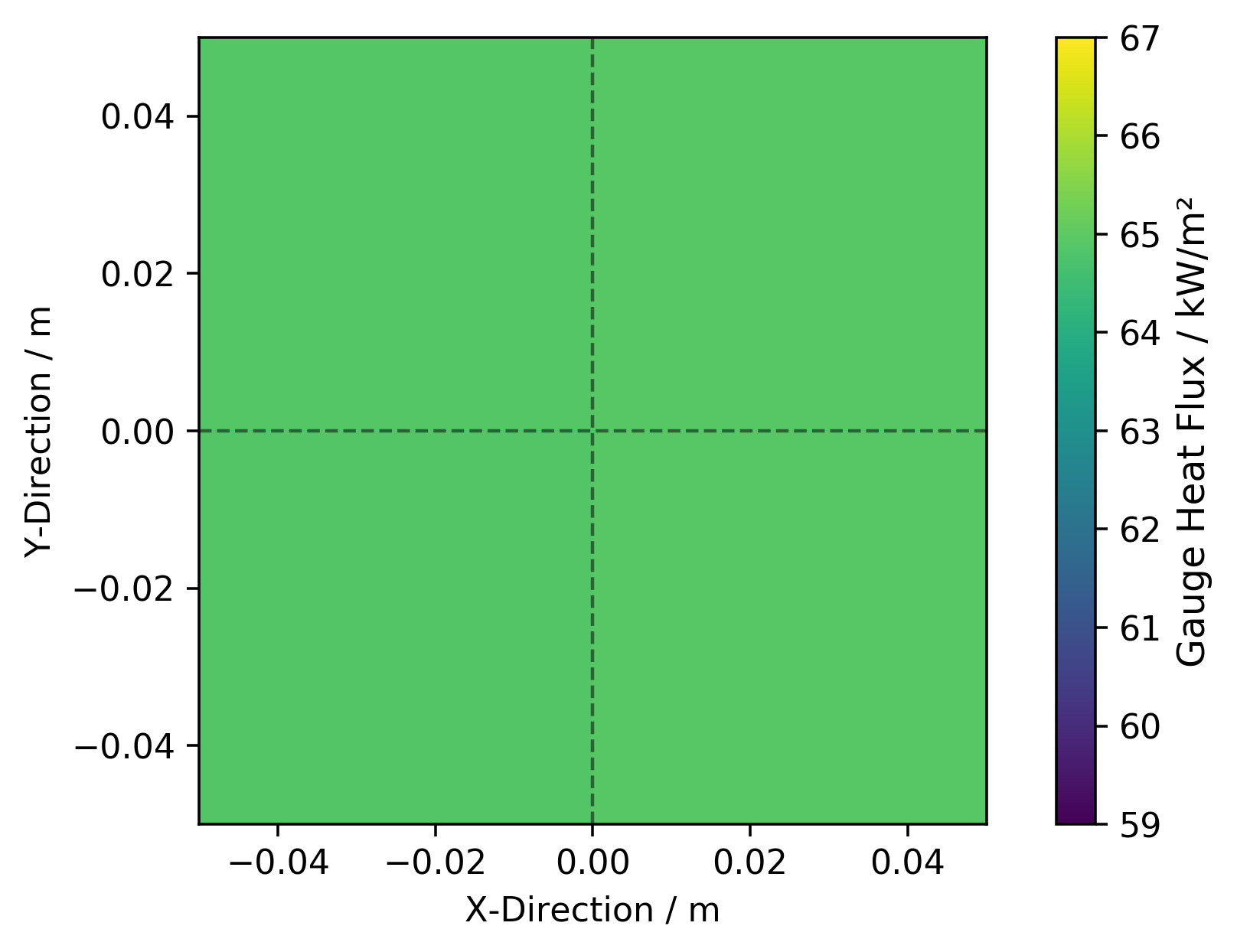
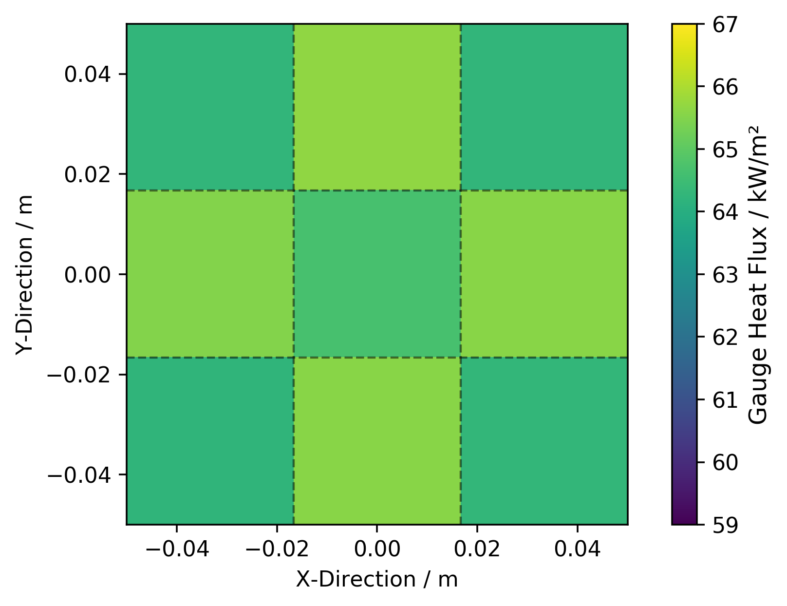
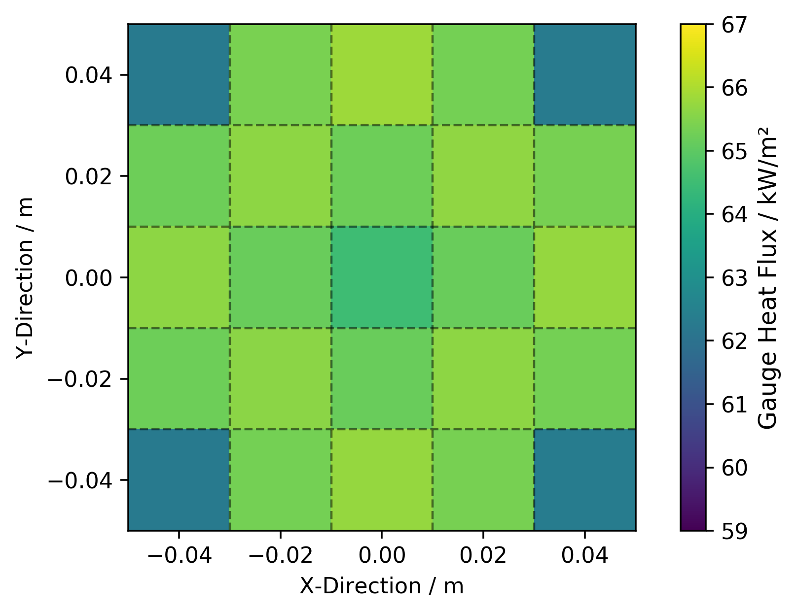
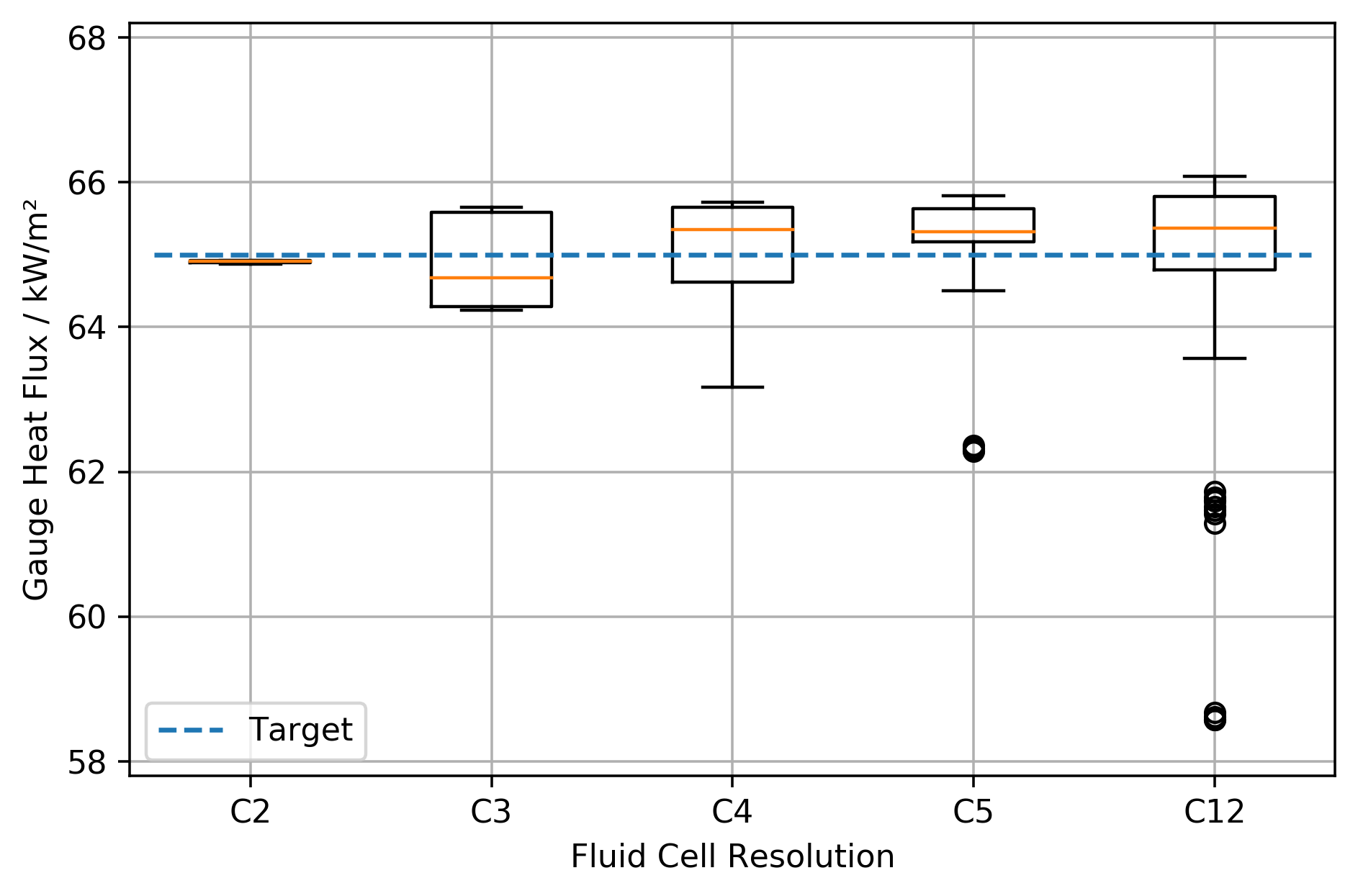
The radiative heat flux of the heater is imprinted to the sample surface in the low resolution setups, such that a heater model can be neglected. This radiative heat flux is determined by employing a high resolution simulation (C12) containing a geometrical model of the heater, see appendix section A. The model is designed based on information in the literature [46, 47]. The resulting heat flux distribution on the sample surface is recorded (GAUGE HEAT FLUX), see figure 9. It is observable, that the radiative flux is not uniform across the sample surface, as was also reported earlier [25, 26, 48]. Based on the fluid cell size of the respective the IMP (C2, C3 and C5), low resolution maps are computed, see figure 10. These maps are implemented, using multiple surface definitions with different heat flux values (EXTERNAL_FLUX) for the individual sample surface cells.

4.2 Results

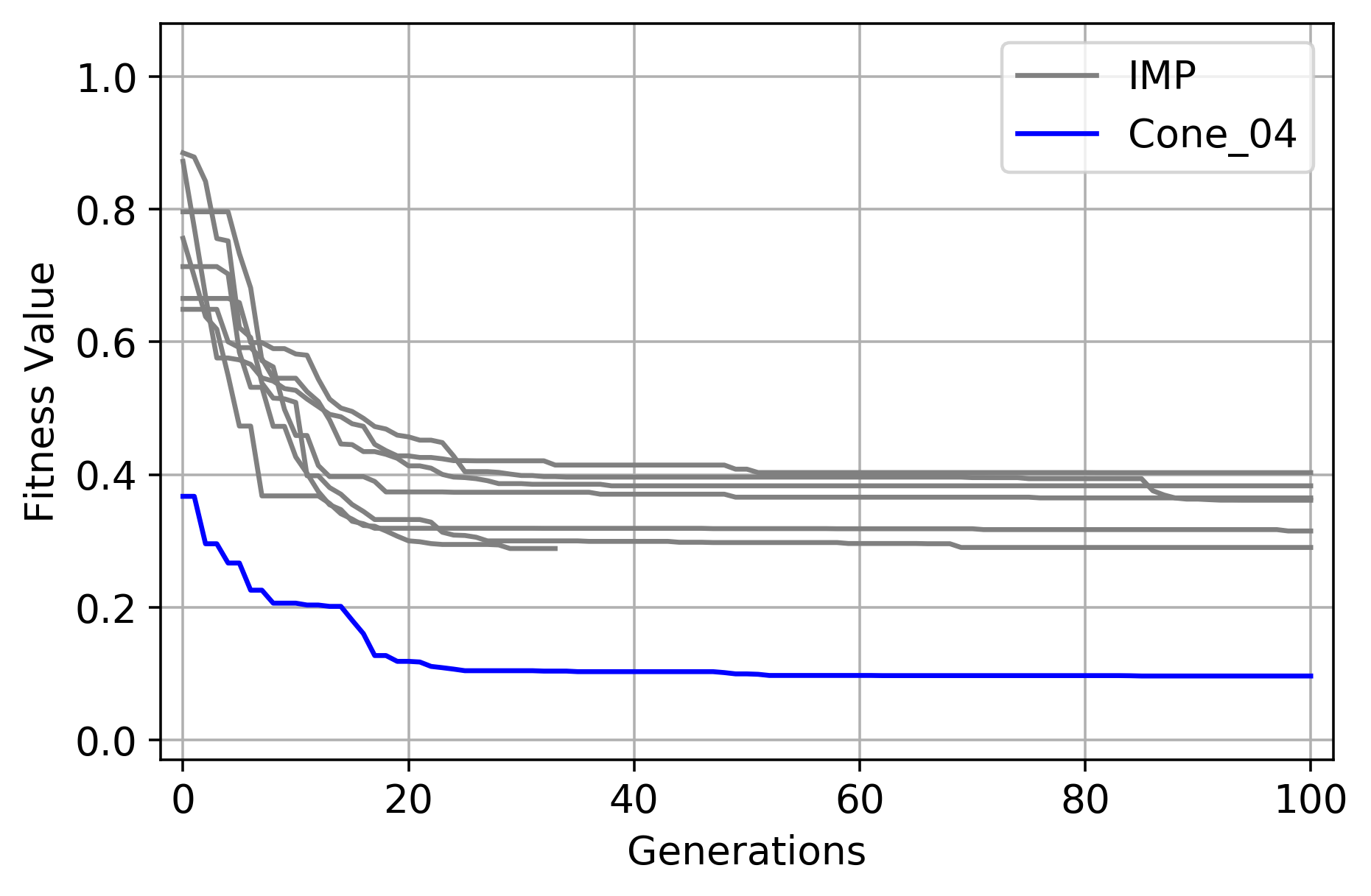
Here, an overview of the simple cone calorimeter IMP results of the best parameter sets is presented. The full data is provided in appendix G for completeness. The best fitness values of the IMP runs are summarised in table 6. For each IMP run, 100 generations have been completed, see figure LABEL:fig:IMPConeBestParaC3_fit and figure 31. Cone_04-L3 has the lowest fitness value, but its target is only the energy release, thus it is not directly comparably to the remaining IMPs.

Table 6: Best parameter sets of the different simple cone calorimeter IMP setups. Note: Cone_04 is lower, since it only uses energy release as target, while all others also solve for back face temperature.

IMP Setup	Limits	Repetition	Fitness Value
Cone_01	L2	43718	0.361
Cone_02	L2	38608	0.402
Cone_03	L3	17857	0.383
Cone_04	L3	39571	0.096
Cone_05	L3	13568	0.288
Cone_06	L3	45893	0.314
Cone_07	L2	35532	0.364
Cone_08	L3	32262	0.290

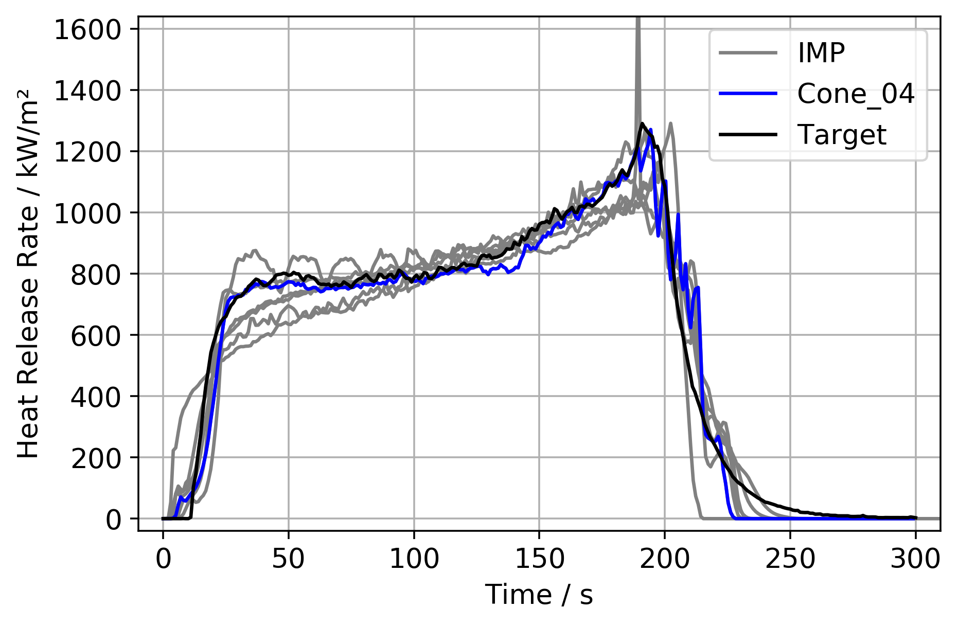
Figure 11 shows the responses of the best parameter sets of all the different IMP setups. For all cases, the optimiser is able to find a parameter set that reproduces the experiment data relatively well. This is emphasised by drawing all their responses without distinction, including different fluid cell resolutions (C2, C3 and C5). Cone_04 is highlighted, because it uses only the heat release as target.

With respect to the heat release, difficulties exist in reproducing the first bump at around 20 s to 50 s, the final peak at about 190 s and the following decay phase. In some cases, pronounced steps are visible towards the end of the simulations. See for example figure 32 for Cone_06. These steps are associated with the burn-out of the individual cells. Furthermore, in all cases a small peak is visible in the beginning of the cone calorimeter simulations, at about 15 s. Cone_04 and Cone_08 capture the heat release profile best (figure 32).

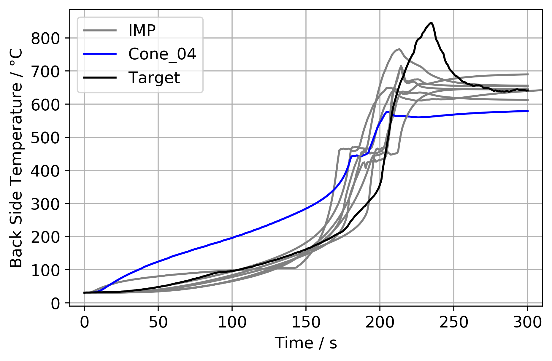
Reproducing the temperature recorded at the back face of the sample proves to be challenging, see figure LABEL:fig:IMPConeBestParaC3_bft and figure 33. For cases where it is a target, the temperature development during the first about 160 s can be reproduced. Between about 160 s to about 270 s departures are visible, with a pronounced step around 200 s. A peak can be observed towards the end, yet less pronounced as in the experiment. Cone_04 does not have the temperature development target and is not able to reproduce a similar behaviour on its own.

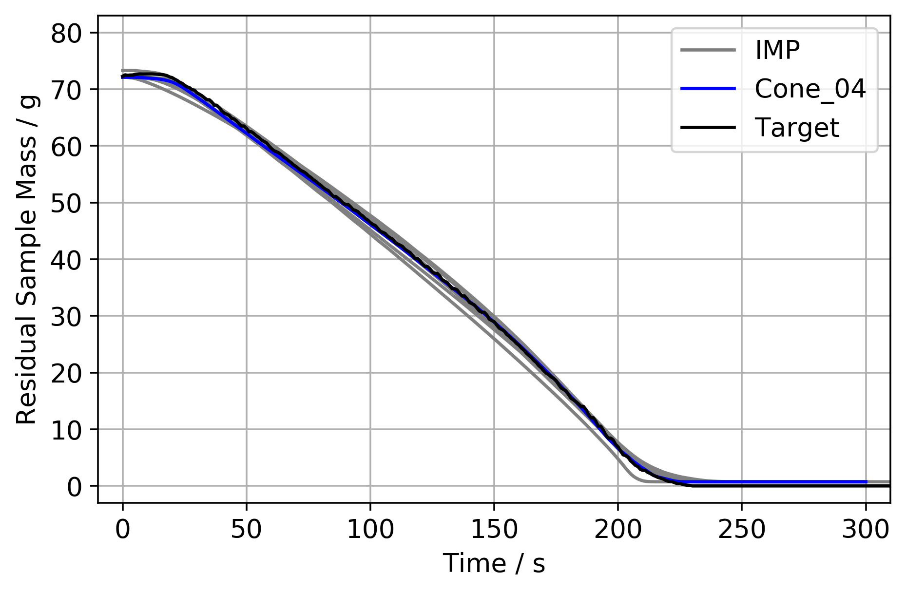
The residual sample masses during the simulation are close to the experiment data, see figure LABEL:fig:IMPConeBestParaC3_mass and figure 36.

4.3 Discussion

In terms of the fitness value, Cone_08-L3 and Cone_05-L3 performed best across all IMP setups, see table 6 and figure 31. This is excluding Cone_04-L3, because it neglects the back side temperature. Adjusting the sampling limits leads mostly to better parameter sets. Occasionally, the IMPs do not find better sets within the given amount of generations. For example, L1 of Cone_03 shows worse fitness values throughout, compared to L0, see 31. The likely reason is that with each adjustment the process starts anew, combined with the randomness for choosing the individual values. With more generations, better parameter sets may be found. The impact of smaller fluid cells during the IMP is not clear. It might lead to better parameters for the Cone_05 series, yet its enormous runtime makes it not feasible to wait its completion during this work. As of now, it shows fitness values that are just marginally better than Cone_08-L3 (table 6).

Compared with previous work, e.g. [8, 10], here, higher fluid cell resolutions are used to cover the cone calorimeter sample. With C3 and above, the cells become distinguishable between corners, edges and centre cells — compare the flux maps for two, three and five cells (figure 10). For the C2 configuration, each cell has essentially the same value – the average over the whole surface. This is summarised in figure 12. Higher resolutions capture the ring-shaped pattern of higher heat flux in the centre and the substantially lower heat flux in the corners better, see figure 9. The steps in the simulations during the decay phase might be a result of it, see figure 32 between about 200 s to 250 s for Cone_06_L0. Two processes control the decay: cells burning out and the local burning behaviour, depending on the material parameters. Combining both can smooth out the decay phase. This combining is difficult to achieve without an optimiser, because the parameter set needs to behave as if three-dimensional heat transfer is possible even though it is not. The C2 cases are primarily controlled by the parameters and show a steep drop at the end (Cone_07), because uneven sample consumption cannot be covered well. In the C3 setups the formation of pronounced steps is visible in some L0 cases, but higher limit adjustments can show a smoother decay. During the IMP a fluid cell resolution of C3 seems to be beneficial. It allows to capture the uneven heat flux to the sample surface, distinguish between cell locations and also provides a better resolution of the flow and radiation fields. Higher resolutions are computationally very expensive, specifically within the constrains provided by the SCE.

This behaviour is also reflected in the back side temperature. During the decay period a spike is visible (figure LABEL:fig:ConeExpAalto_temp), until the temperature settles at a constant value, from around 280 s onward. This constant value primarily shows the influence from the heating element, without the sample. During the experiment, the sample material is consumed and at some point the thermocouples below are exposed, starting from the centre. Thus, they are able to receive the heat radiation from the flame of the surrounding sample directly, in addition to the heater radiation. Due to thermal tension, they may also bend towards the heater. All these aspects together lead to the formation of the spike.

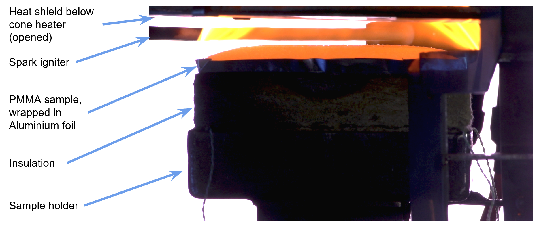
The optimiser has difficulties to capture both, the heat release rate and the material temperature. With lower fluid cell resolution (C2, Aalto_6b in figure 33) the temperature peak between 200 s and 250 s cannot be reproduced. This is associated to the near-uniform consumption of the sample material, see above. In the other setups, the peak can be captured for the initial sampling limits, but mostly disappears with further adjustments. Certainly, neglecting three dimensional heat conduction inside the sample, is influencing the outcome as well. On the other hand, the sample shape can change significantly during the experiment, see figure 13. Relatively early on, it creates a foam layer and starts to bend towards the heater. In similar experiments performed by Karen De Lannoye, the maximum height of the bump was observed to extend approximately two sample thicknesses above the original surface of a sample with a thickness of 6 mm (figure LABEL:fig:PMMAsampleDeformationCropped, right), but the behaviour can change depending on the experiment conditions [49]. This relatively symmetrical bump can change its shape significantly during its decay. While the sample material is consumed, its surface retracts further away from the heater, compared to the beginning of the experiment. Thus, in the experiment, the received radiative flux from the heater should change. These deformations are not replicated in the simulations presented here – the component of the radiative flux of the heater stays constant, by construction. Only the heat flux component from the flame can change. The sample deformation is likely misinterpreted as a change in mass and energy release during the inverse modelling.

Given the deformation, it is fundamentally unclear where the back face temperature is actually recorded. Furthermore, changes in the rigidity of the PMMA sample (e.g. melting) such that the thermocouple tip can move into the sample, thermal expansion of the sample holder assembly and associated movement between individual components, mechanical tension on the thermocouples and others are contributing to the uncertainty. Assuming they would be tightly attached to the backing material, an air gap could form between them and a bent sample. Such a gap would be interpreted as lower thermal conductivity during the IMP. As an example, compare Cone_04 with the other IMP results in figure LABEL:fig:IMPConeBestParaC3_bft. It only uses the energy release as target, not the back side temperature. The temperatures are higher throughout the simulation. Curiously, in the parallel panel simulation setup this behaviour appears to be beneficial, as discussed later in section 5.3. This seems to hint at incorrect temperature readings during the cone calorimeter experiment. If the sample separates from the thermocouple due to deformation, its recorded temperature should be lower than the actual back face temperature. Consequently, higher back face temperatures are visible in Cone_04 (figure LABEL:fig:IMPConeBestParaC3_bft), since in the simulation it is recorded at the back face of the sample by construction. From the above, the uncertainty of the recorded temperature increases during the run time of the experiment. Reliable temperatures might only be able to be recorded for low sample temperatures during the beginning. Specifically considering the deformation, melting and consumption of the sample. Therefore, the intended separation between sample behaviour and the boundary conditions could not be achieved.

In the future, it would be interesting to assess the surface deformation of the sample during cone calorimeter tests. Maybe one could leverage methodologies used in assessing the performance of intumescent coating, e.g. [50]. This could then be used to adjust the prescribed radiative heat flux to the sample surface over time.

The conductivity and specific heat change with sample temperature in the simulation (RAMP). This can account for the sample deformation to some degree, when an air gap forms between sample and thermocouple. The temperatures are arbitrarily chosen and used for both parameters, except for Cone_02. At high temperatures Cone_01, 03 to 05 get relatively high values assigned by the optimiser, see figures 34 and 35. Since the material is consumed way before the 800 °C could be reached, only a very small fraction of the ramp piece between the last two points can meaningfully contribute. Thus, ramp values for 800 °C are poorly chosen and should be disregarded. The cases where the temperature points are chosen based on the MCC experiment data, see figure 8, lead to more reasonable results for the conductivity, which is different for the specific heat. The final point is at a temperature close to the maximum the sample material can reach. Still, it seems to be a useful approach for unknown materials to align both temperature dependent values to the micro-scale data. Maybe the highest temperature value of the ramp could be chosen to be about 20 K lower than the highest meaningful value in the experiment data. This is an attempt to prevent confusion of the optimiser with temperatures that are impossible to reach, because the material is consumed. Another strategy could be to run an IMP solely to determine the ramps for some best parameter set. Thus, more parameters could be spent on the ramp alone without getting too large generation sizes.

With data provided from DBI/Lund [7], extending the conductivity ramps in Cone_08-L3 seems not to change the temperature development significantly, see figure 34. For most of the IMP setups, values for the lower temperatures are determined that are already in the vicinity of the experiment data.

Overall, the sample mass loss during the cone calorimeter simulation is relatively close to the experiment data, see figure 36. This behaviour is an emergent phenomenon of the steps taken with the gas mixture and gives confidence into the proposed method, since it is not an explicit target of the IMP. However, the flame height and gas temperature change with the release of the different surrogate fuel species, see appendix D. This is likely due to dilution of the surrogate fuel with carbon dioxide. Which of the presented centre line gas temperatures in figure LABEL:fig:FlameHeight_Temperatures is more realistic in context of the PMMA cone calorimeter experiment studied here is unclear for now. Still, it is worth noting that the difference exists, because higher flames might have an impact on the fire spread in a simulation.

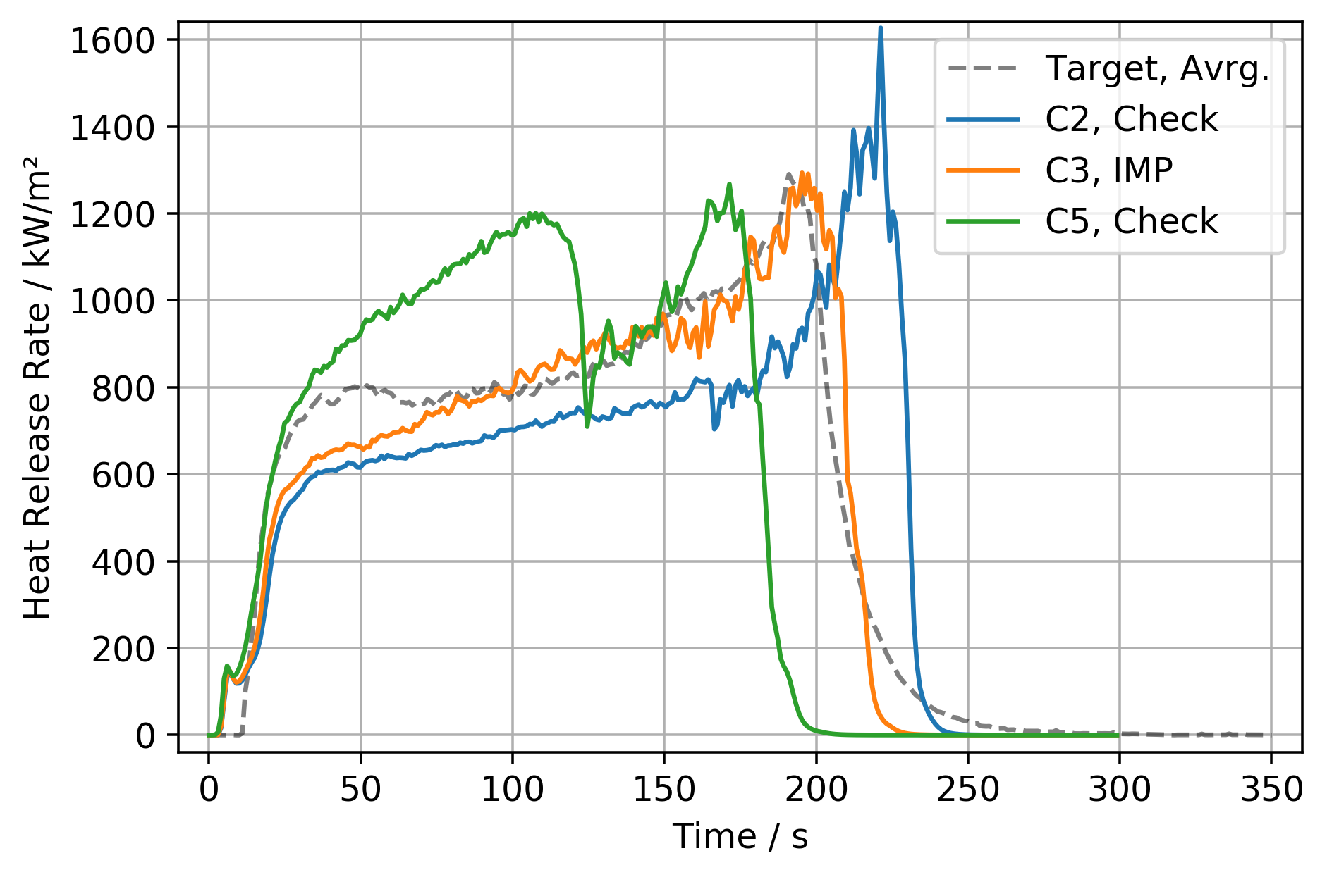
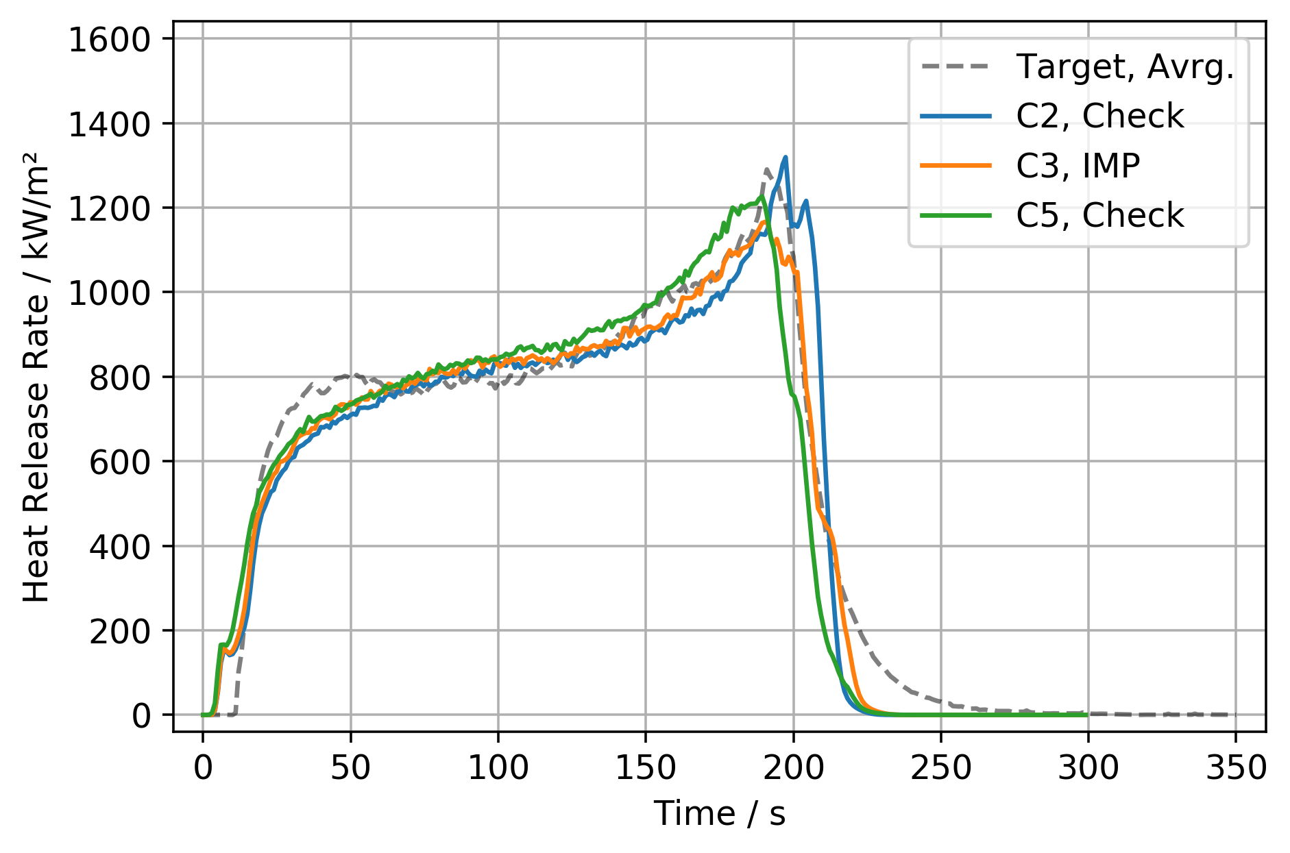
For the IMP, the fluid cell resolution of 3.3 cm (C3) seems to be beneficial. It is able to capture the uneven sample consumption, yet it runs relatively fast. However, the question arises, how will the parameters perform at higher resolutions. For this, figure 14 demonstrates an exemplary comparison: a parameter set determined at a given resolution (labelled "IMP") is used at an other resolution (labelled "Check"). Some of the investigated cases show similar behaviour across all limit adjustments, see figure LABEL:fig:SimpleCone_CellSize_Comparison_Aalto5L0 and figure LABEL:fig:SimpleCone_CellSize_Comparison_Aalto5L3. Others converge towards the higher resolution over the course of multiple limit adjustments, see figure LABEL:fig:SimpleCone_CellSize_Comparison_Aalto4L0 and figure LABEL:fig:SimpleCone_CellSize_Comparison_Aalto4L3. All limits are provided in appendix H. Given the reduction in computational demand, this is promising.

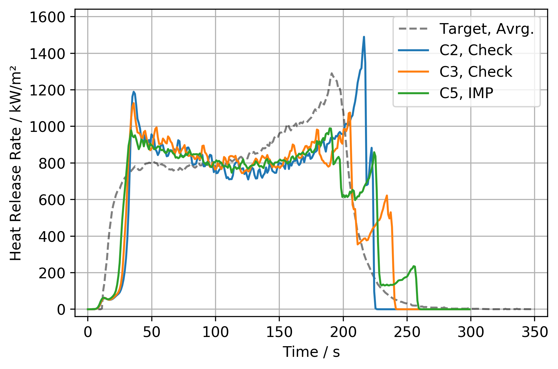
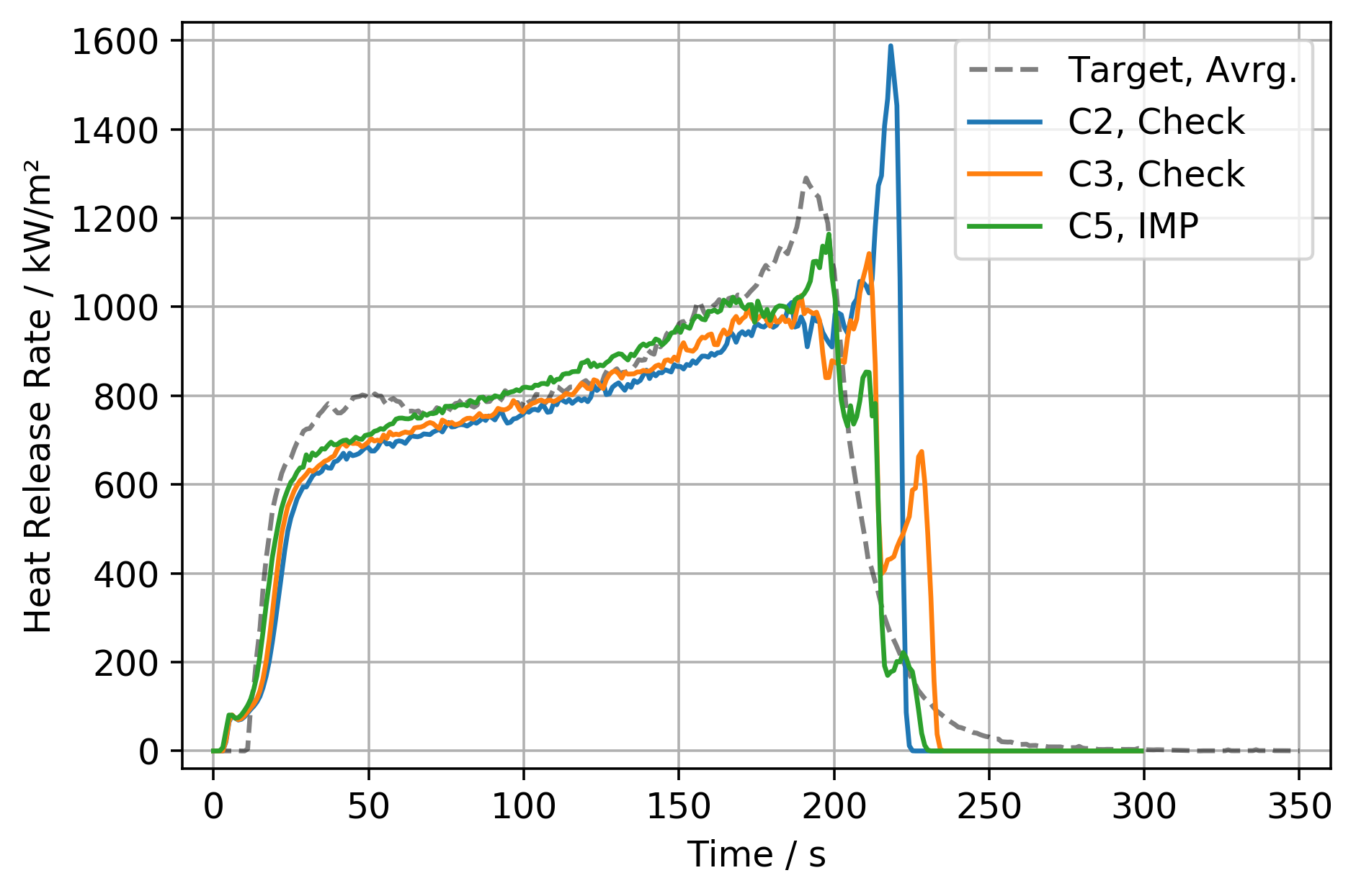
The overall runtime of this IMP step is a notable limitation for practical usage. Given the development of the fitness values for each of the IMP runs, one could consider to run less generations. Possibly 60 to 80 generations could be sufficient. Furthermore, using less parameters during the IMP has a strong impact on the amount of simulations necessary, see equation 1. Maybe the parameters of the backing could be determined in an individual step. Using data from differential scanning calorimetry, the specific heat capacity could be determined in the less costly first IMP step. Optimising this second IMP step needs further investigation.

5 Real-Scale Setup — Validation

5.1 Methods

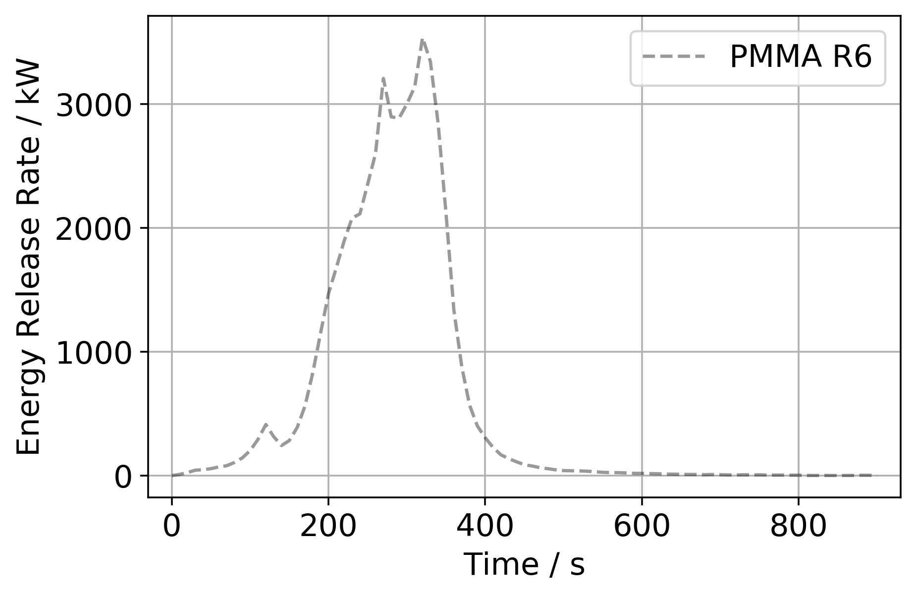
As a validation step, the material parameter sets (table 6) are used in a real-scale simulation setup of a parallel panel test. The results are compared to the heat release rate measured in the experiment, see figure 15. The data set used here is "Test_7_PMMA_R6", labelled "PMMA R6" [27].

The parallel panel test consists of two 0.61 m wide panels facing each other with a separation of 0.3 m. In between both, at the bottom, is a gas burner located with a width of 0.3 m and a length of 0.61 m, see validation guide [44] cases "FM Parallel Panel Experiments" and "NIST/NRC Parallel Panel Experiments", as well as the MaCFP data base [27]. The combustible sample, attached to the inside of the panels, extents 2.44 m above the burner surface. The burner is fed with propane gas. It reaches a quasi-steady energy release of about 60 kW, between 60 s to 80 s after its ignition. After the sample is confirmed burning (sustained flaming across the panel walls), the burner is shut off. This happens about 120 s after the start of the experiment. Shutting the burner off slows down the fire development for about half a minute, see figure 15 between about 120 s to 150 s. The sample material is the same cast black PMMA used throughout the MaCFP test campaign.

The simulations are conducted for the three different fluid cell resolutions introduced in section 4.1. The computational domain spans a volume of 1.2 m $\times$ 0.8 m $\times$ 4.8 m and is divided into multiple sub-domains (MESH), with the following divisions along the x, y and z axis: (3, 1, 12). A graphical overview over the domain layout is provided in appendix B, figure 25. Thus, the individual mesh dimensions are multiples of 10 cm and can be nicely divided following the scheme outlined in section 4.1. This number of meshes allows the simulation to be run on a single computing node, utilising its 64 cores. The simulation mode is set to LES.

The surface definitions are taken from the "NIST/NRC Parallel Panel Experiments" validation case, associated with FDS6.7.6-810-ge59f90f-HEAD. The sample material definitions are built from the parameter sets created within this work. Propane is used as fuel species for the gas burner in the simulation. This differs to the FDS validation setup "NIST/NRC Parallel Panel Experiments", where the combustion reaction for MMA is used for the burner and the sample. Note, the respective case was updated recently for FDS 6.8 and up. In contrast to the experiments, during the simulation the gas burner is kept at a continuous heat release of 60 kW throughout, releasing a mass flux of about 0.00732 kg/(m² s). Shutting the burner off earlier leads to fire extinction relatively fast, see discussion in section 5.3.

5.2 Results

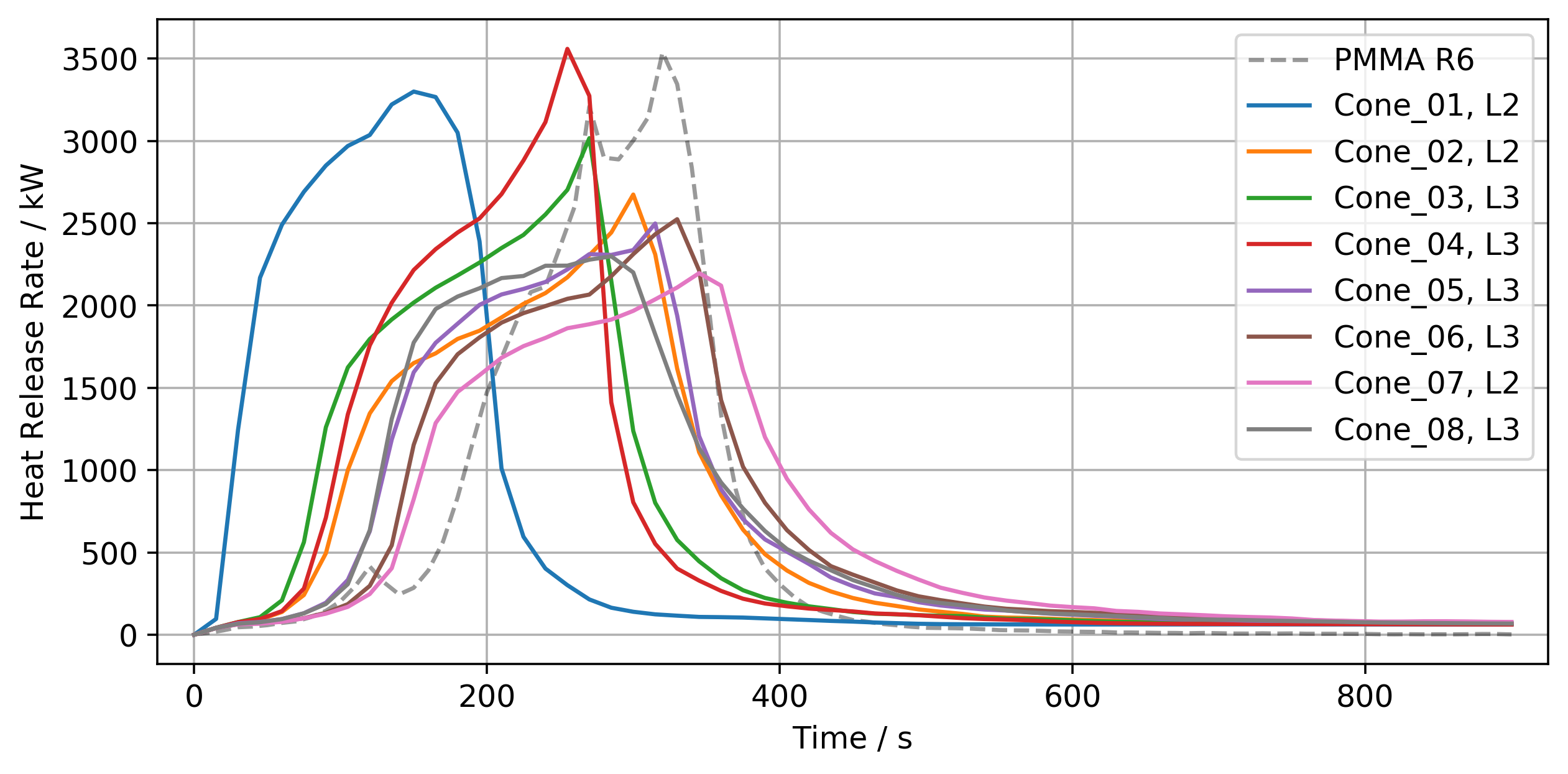
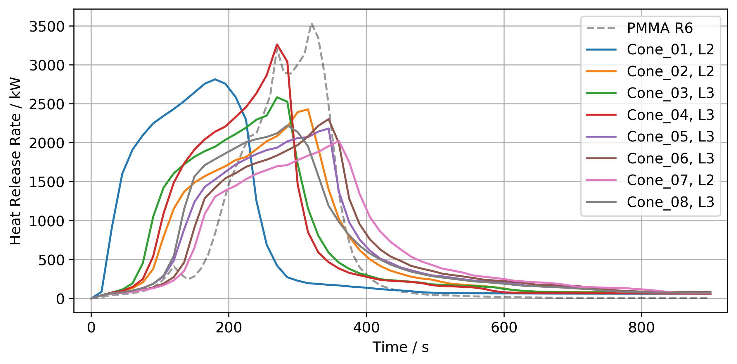
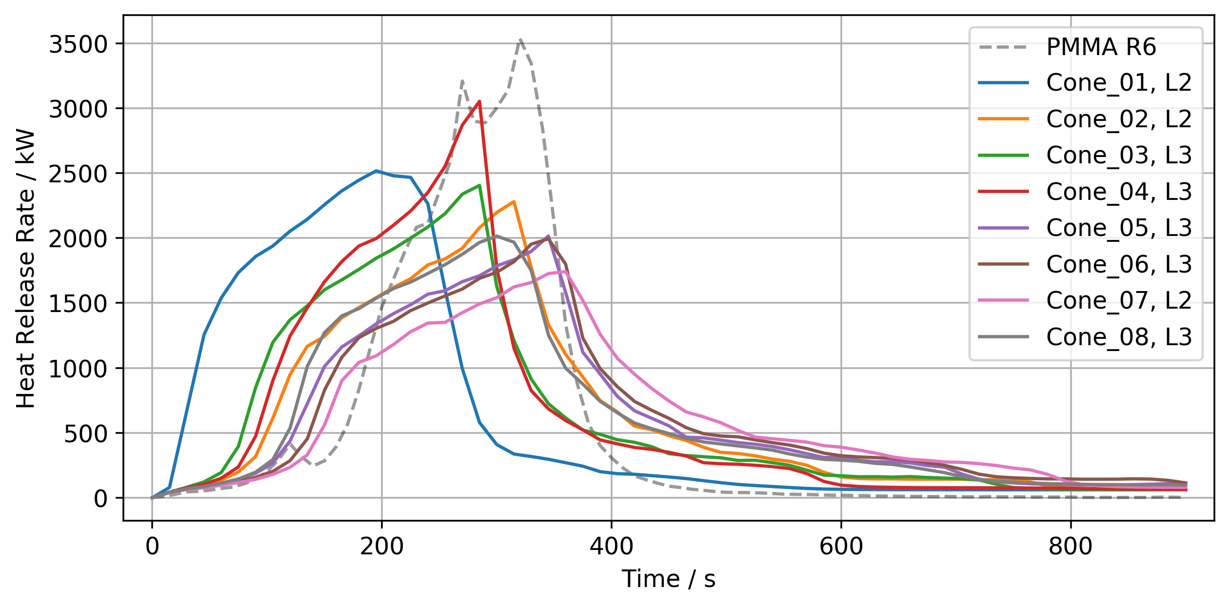
The heat release rates in the parallel panel simulation setups are presented in figure 16.

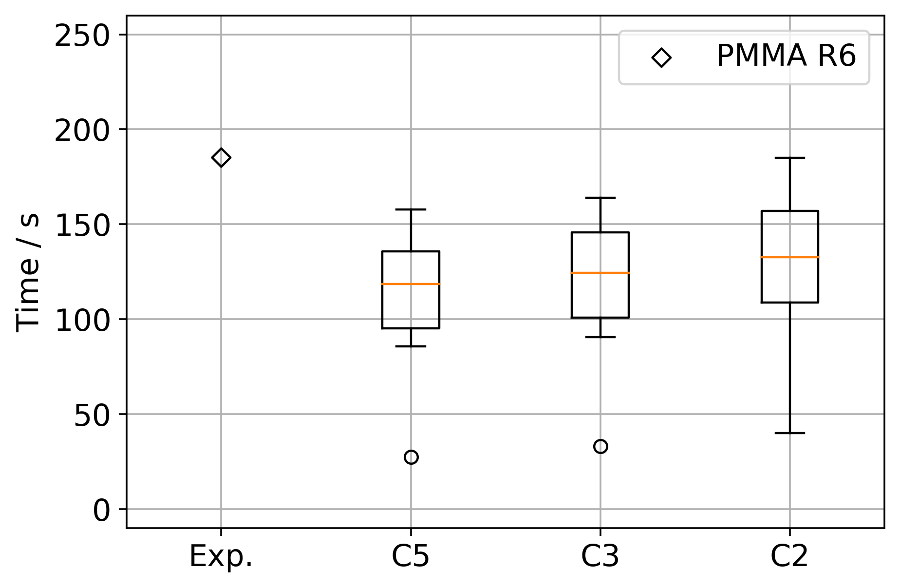
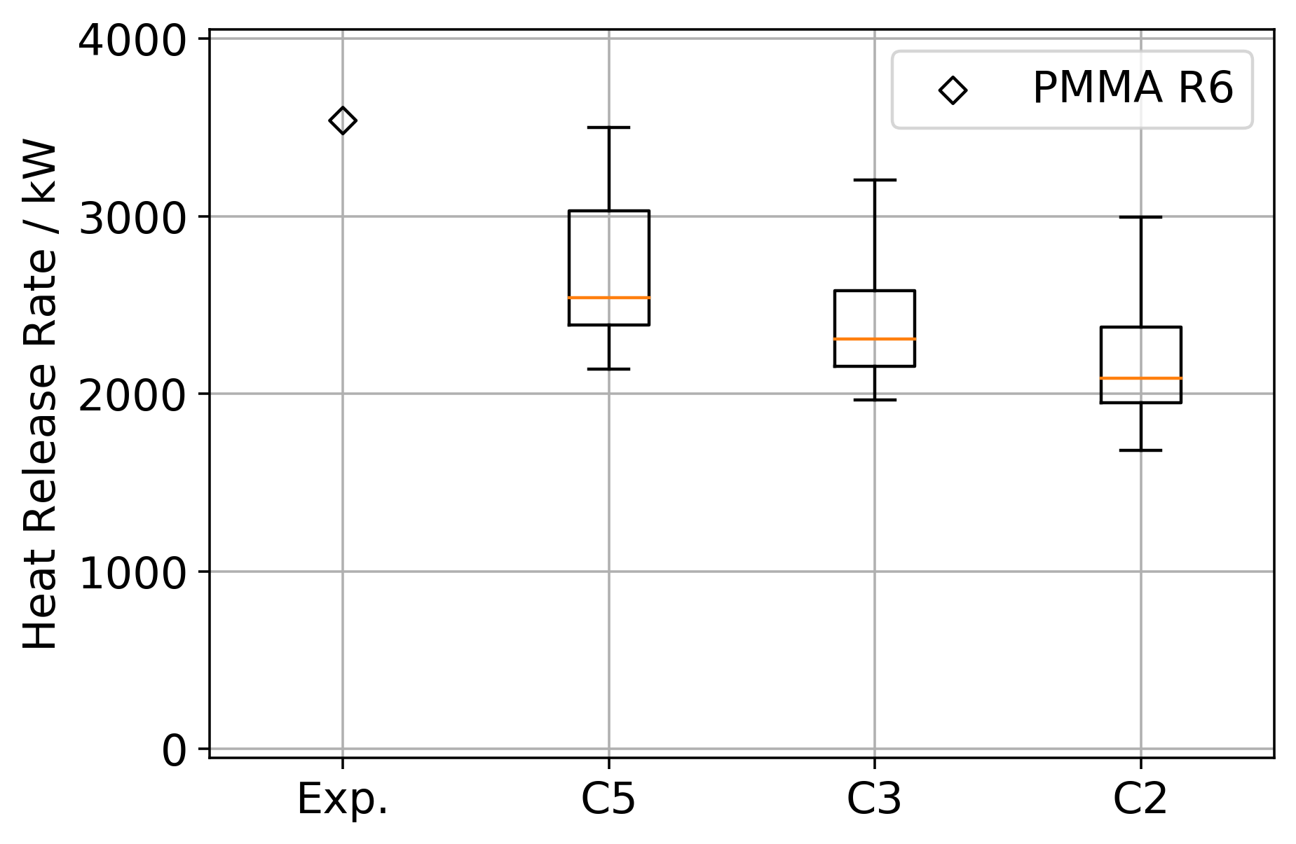
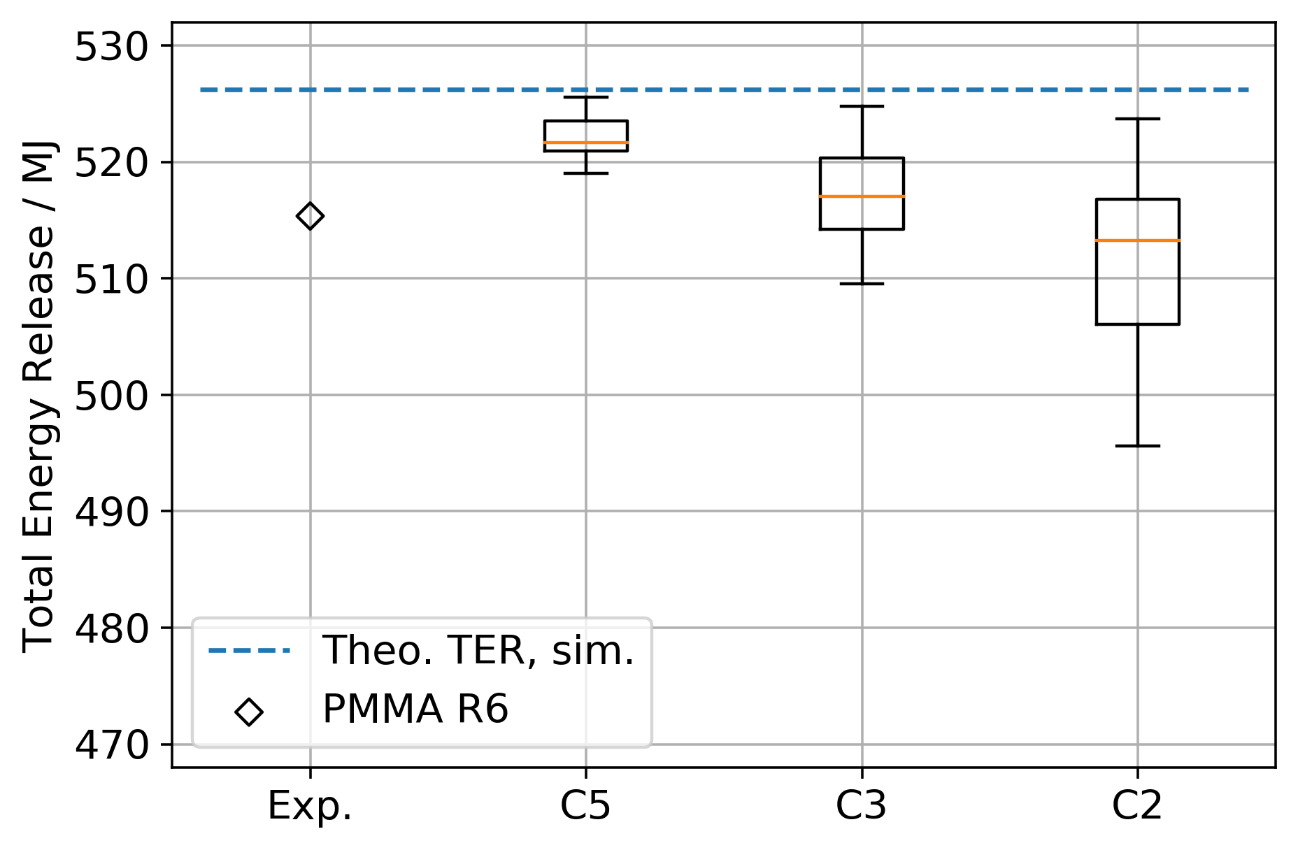
For the smallest fluid cells (C5, figure LABEL:fig:PP_BestHRR_20mm_RF30), the peaks are overall narrower and taller compared to the largest cells (C2, figure LABEL:fig:PP_BestHRR_50mm_RF30_C2). This is emphasised by comparing the peak energy release, see figure LABEL:fig:PP_BaseAssessment_Peak. In the simulation the fire develops overall faster compared to the experiment emphasised by the time a HRR of 1 MW is reached, see figure LABEL:fig:PP_BaseAssessment_1MW. Larger cells slow the development down slightly. In general, faster fire development leads to higher energy release, see figure 18. The total energy release (TER) of all parallel panel simulations with different radiative fractions of the propane combustion reaction is provided in figure 38 in the appendix.

5.3 Discussion

With the real-scale setup, the performance of the best parameter sets of the different IMPs (table 6) is assessed.

The fire development in the simulation is faster than the experiment for all parameter sets and fluid cell sizes, see figure 16. This could be related to the faster ramp-up of the burner in the simulation. It takes 10 s to reach the desired heat release, compared to the 60 s to 80 s in the experiment. Also, the burner is kept burning throughout the simulation, because the fire would extinguish otherwise (see below). Shutting the burner off in the experiment leads to a visible delay in fire development, see figure 15 between about 100 s to 200 s. With larger fluid cells the overall fire development is more drawn out. This could be related to a poorer resolution in the radiation field, since for example the radiation angles are not adjusted, using the FDS default of 104 solid angles. This is also reflected in the TER, indicating that less sample material is consumed than in the experiment, see figure 18. Overall, smaller fluid cell sizes, specifically C5, lead to HRR peak shapes with closer resemblance of the experiment data. With the chosen model settings here, the fluid cell resolution should be C5 or higher. Throughout all parallel panel simulations, Cone_07 performs the worst. It uses the largest fluid cell size during the IMP. However, its performance may also be influenced by its IMP target, i.e. using the HRR and the back face temperature. This should be investigated in more detail in future work.

The peak heat release is about 30% to 40% lower in the simulation, depending on fluid cell size and parameter set, see figure LABEL:fig:PP_BaseAssessment_Peak. A notable exception is the parameter set of Cone_04. Its performance stands out, by most closely resembling the shape of experiment "PMMA R6" and reaching a similar peak HRR. This behaviour seems to be associated to neglecting the back face temperature as IMP target in the simplified cone calorimeter setup. In future work, it is worth to look in more detail at Cone_04. Removing the back face temperature constraint seems to be beneficial for the real-scale and may be improved with better chosen temperature values for the ramps.

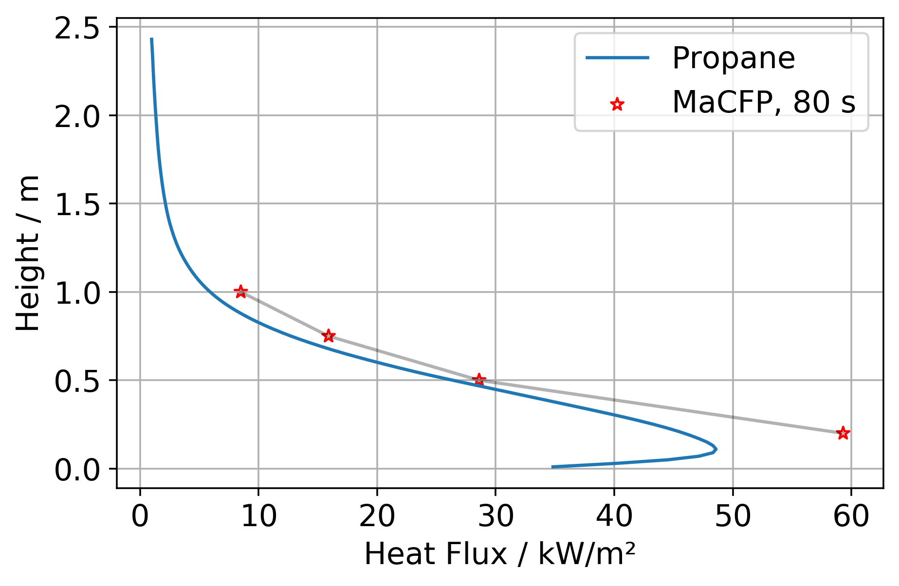
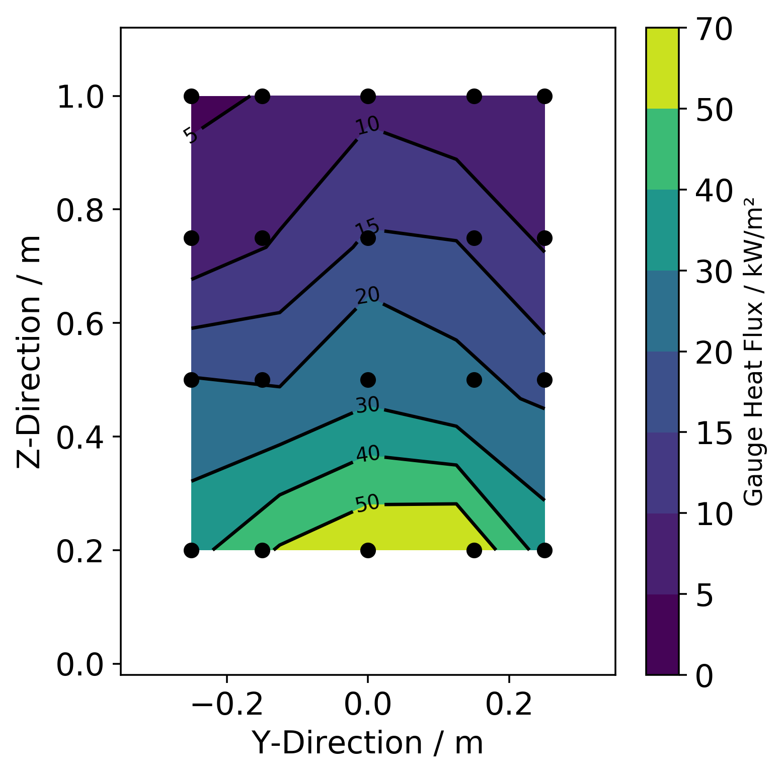
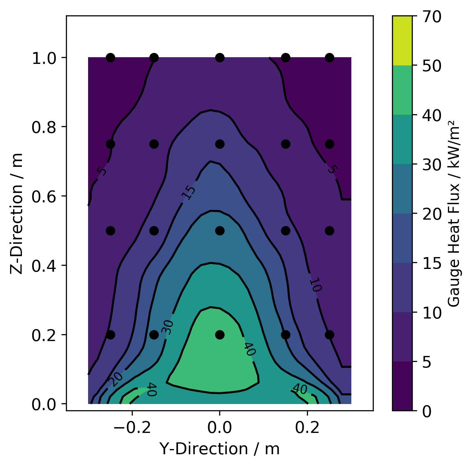
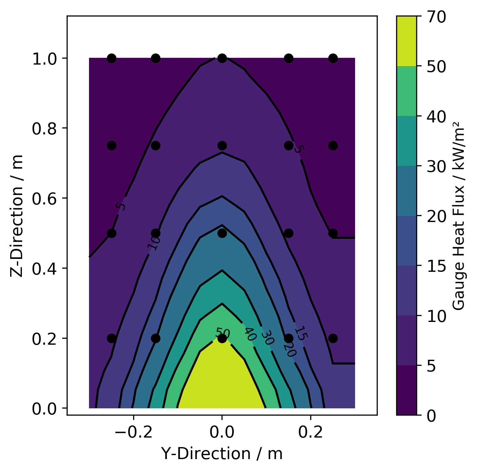
During the work presented here, only the flame heat flux along the vertical centre line of the empty panels is taken into account as starting condition (figure 19). More detailed data was recently made available via MaCFP [27]. Unfortunately, this was too late to be taken into account for the conducted simulations here. Even though the simulations could not be changed anymore, the flame heat flux data across the lower part of the empty panels is compared against simulation responses for the different fluid cell resolutions, see figure 20. All four plots show flux data averaged over 20 s during the steady-state. The dots show the device locations during the experiment. From the simulation, the heat flux is extracted from the solid boundary directly (GAUGE HEAT FLUX). In the experiment, the flux is spread out nearly horizontally along the panels (figure LABEL:fig:PP_HeatFluxMapExp). While in the simulation, it is more focused towards the centre line, which coincides with the location of the simulated flame (figure LABEL:fig:PP_HeatFluxMapSimC5). With larger fluid cells, the heat flux is more concentrated at the lower centre line (figure LABEL:fig:PP_HeatFluxMapSimC2). This indicates that the initial conditions are not reproduced well. It is not sufficient to simply match the heat flux to the vertical centre line of the panels. To properly assess the performance of the parameter sets, the burner itself needs to be accurately modelled first. For future work, it is necessary to develop a more comprehensive representation of the gas burner setup. Further investigations should incorporate the impact of simulation parameters like soot production, cell sizes, parameters of the radiation model and material parameters of the burner top face and empty panels.

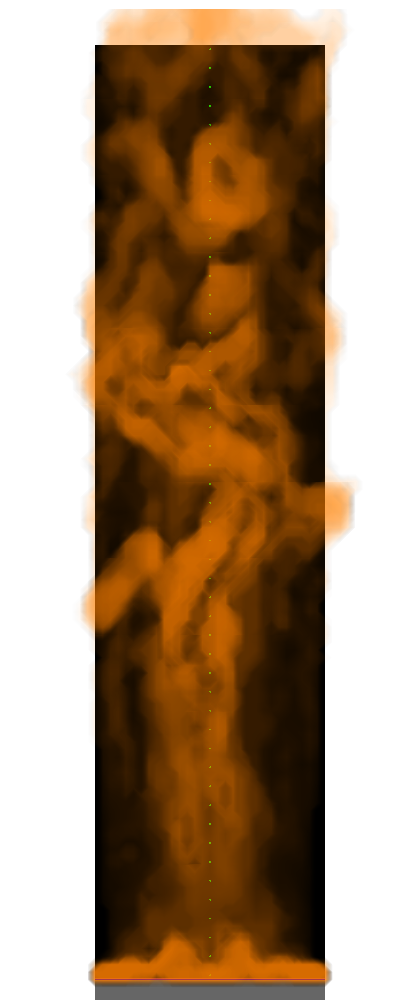
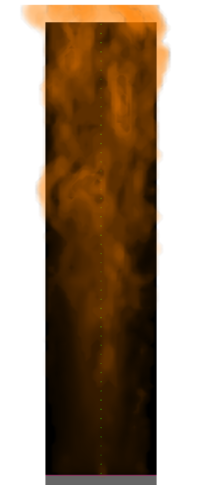
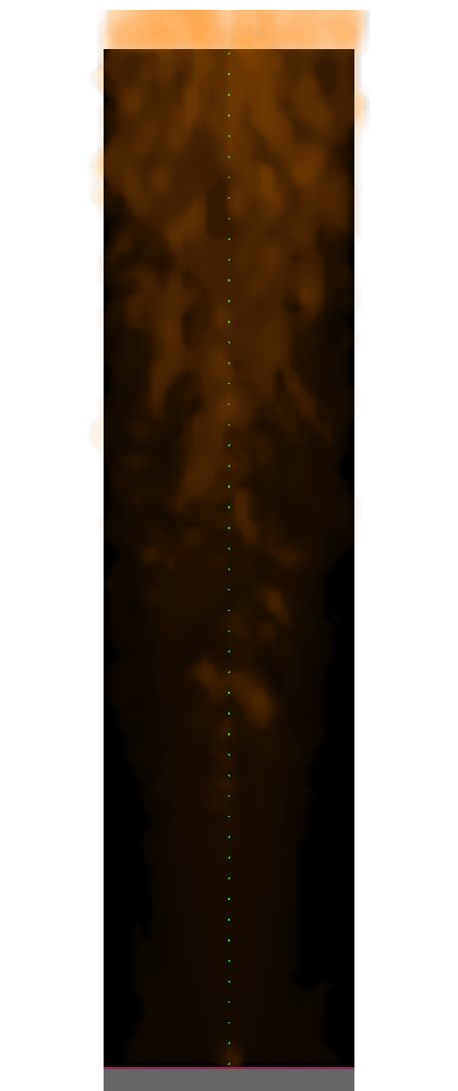
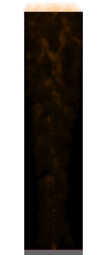
Simulations with different burner cut-off times have been conducted to assess the capability to predict self-sustained fire development. Burner cut-off times of 120 s and 220 s are chosen. In all cases the fire is not able to recover, see figure 39, even though the peak energy release in some cases is in excess of 1 MW. As an example, figure 21 shows an image of the experiment "PMMA R6" [27] and an image series captured in Smokeview, covering 60 s after the burner is shut off. The flame region is flat against the panels, about one to two cells. This might interfere with the radiative heat transfer to cells below the lower edge of the flame, as well as to the sides. A closer look at the parameters of the FDS radiation model might be necessary, for example the path length or number of radiation angles. Smaller fluid cells might be beneficial as well, due to a better resolution of the resulting temperature distribution in the combustion region. It should be noted further, that the radiative fraction for combustion reaction of the PMMA pyroylsis products is treated here as unknown and the FDS default is used, i.e. 35 %.

Overall, there is a clear need to investigate the conditions necessary for self-sustained fire spread in the real-scale simulation and the parameter transfer from micro- to bench-scale and further from bench- to real-scale. In the given setups here, the model seems to struggle to provide meaningful energy transfer to the cells around the combustion reaction zone to keep the flame. Additionally, the impact of environmental effects on the experiment needs to be quantified or reduced, e.g. by conducting multiple repetitions of the same experimental setups.

6 General Discussion

All IMP results are able to reproduce the chosen micro-scale setups and cone calorimeter data well, see figure 4, 5 and figure 11. Yet, in the parallel panel simulation, differences become apparent, see figure 16. Just from the cone calorimeter simulation results alone, it is not obvious how the parameter sets perform in the real-scale. Preliminary investigations indicate that individual parameters of the material model may be differently sensitive to the simulation and experiment setup [51]. In the cone calorimeter setup fire spread is negligible, specifically for higher radiative heat fluxes. This might mask the behaviour of some parameters. For example, the emissivity has certainly a high impact on the received energy and therefore how the sample material heats up. However, in the cone calorimeter the sample receives a constant and high flux, which might be high enough to heat up the sample fast, regardless of which value for the emissivity is chosen.

In [21] the authors discuss similar observations. They state that for their real-scale simulations, the prediction of the fire development is of lower accuracy, despite the good reproduction of the micro- and bench-scale seups [15]. They state further that small changes in the specific heat capacity of the PMMA material have a large impact to the HRR in their model, specifically in the uncoupled setup. They mitigate this by adjusting the specific heat capacity, as well as the imprinted fractions of convective and radiative heat transfer for the individual surface elements.

The energy transfer to the sample has a significant impact on the fire development. Specifically for the cone calorimeter setup the thermal radiation is important. More detailed investigation of the impact of the radiation model parameters in this setup is necessary. This assessment should also take the performance in the real-scale simulation into account, to ensure that the model for both setups is the same. More care should be taken when setting up the gas burner simulation model. Using individual gas phase combustion reactions for burner and sample should allow to simulate the initial sample ignition more precisely, without compromising the overall sample behaviour.

In this work, the energy release is assumed to solely take place as a gas phase combustion reaction. This may be a sufficient model for PMMA. For other materials that show significant surface reactions, like wood, this assumption might not hold.

Furthermore, experimental campaigns should incorporate medium-scale setups that focus on self-sustained fire spread. This allows to test the model specifically on this aspect, which a cone calorimeter cannot provide due to its design and severe condition. It would also be useful to provide more information on the burners themselves. Specifically, their surface temperature development and emissivities over the course of the experiment.

7 Conclusions

In general, it seems attainable to simulate fire propagation in FDS, based on material parameters. Although the material parameter sets lead to similarly good representation in the micro- and bench-scale, they lead to significantly different results in the real-scale. It is highlighted, that the experiments at this scale introduce further modelling parameters, e.g. the characteristics of the ignition source. Thus, the system is not only dependent on the performance of the material parameters alone.

The reasons for the observed deviations in the real-scale simulations may be:

•

Compensation or trade-off effects during the inverse modelling due to the simplified simulation setups at the micro- and bench-scale.
•

Not all necessary physical processes being captured well enough in the real-scale setup. This includes experimental as well as modelling aspects.
•

Parameter transfer from small-scale to real-scale. The simulation setups used in the IMP may be differently sensitive to individual parameters compared to the real-scale setups. If the real-scale is sensitive to parameters which are insensitive in the small-scale, then the fundamental assumption of transferability is compromised.

Employing a gas mixture allows to capture the MCC and TGA experiments and prevents FDS from scaling the mass introduced into the fluid domain. Thus, it is a step towards more physical parameter sets. The higher fluid cell resolution in the simple cone setup, compared to similar studies, can account for uneven radiative heat flux and sample consumption.

A clear limitation is the enormous computational cost and runtime for determining the material parameter sets. We are currently investigating different strategies to significantly reduce the runtime, by using different sampling methods and artificial-intelligence based approaches.

Overall, it seems clear that many parameters on all levels of this endeavour are important, and their influence needs more cohesive investigation. It is not sufficient to focus on the bench- and micro-scale experiments alone. Despite good performance during these simulations, it is not obvious how the parameters perform in the real-scale. It is necessary to look into the whole chain of setups, to understand how well the parameters eventually translate over to the real-scale. Furthermore, the impact of other model parameters, like the radiative fraction, or the radiation model in general, needs further investigation. Finally, the landscape of experimental data is fractured specifically for real-scale setups with the same sample material as in the smaller scales. Within these constrains, the parameter set should yield a response close to the observations in the experiments at all scales. This ultimately means the parameter set needs to compensate for the simulation model and experimental shortcomings, which can hardly be accomplished by a "physical" parameter set, thus it needs to be an "effective" representation.

Data Availability

The experiment data is available from the MaCFP git repositories [7, 27]. The input for the inverse modelling, the results of the IMPs and the scripts used for data processing are provided in a (open access) Zenodo data repository [28]. A video series on how the data processing and inverse modelling is setup and used is provided on YouTube [29].

Acknowledgements

The authors thank Karen De Lannoye, for discussions on conducting micro- and small-scale experiments and the provided images. The authors thank Isaac Leventon, for discussions on conducting the parallel panel experiments. We gratefully acknowledge the computing time granted through JARA (project jjsc27) on the supercomputer JURECA [52] at Forschungszentrum Jülich and through the project on the CoBra-system, funded by the German Federal Ministry of Education and Research with the grant number 13N15497. This research was partially funded by the German Federal Ministry of Education and Research with the grant number 13N15497.

CRediT Authorship Contribution Statement

Tristan Hehnen: conceptualisation, data curation, formal analysis, investigation, methodology, software, validation, visualisation, writing – original draft preparation, writing – review and editing

Lukas Arnold: conceptualisation, funding acquisition, methodology, project administration, resources, software, supervision, validation, writing – review and editing

Appendix A Cone Calorimeter Simulation Setup

Based on Babrauskas’ [46] original report on the development of the cone calorimeter, a simplified geometrical representation of the heating element is created. The simplification is primarily focused on the heating coil, which is represented as a smooth conical surface and not as a wound wire, see figure 22. The fluid cell resolution was chosen, such that the sample surface (10 cm by 10 cm) was covered with 12 by 12 cells. The geometry itself was built in Blender, using the BlenderFDS addon by Emanuele Gissi.

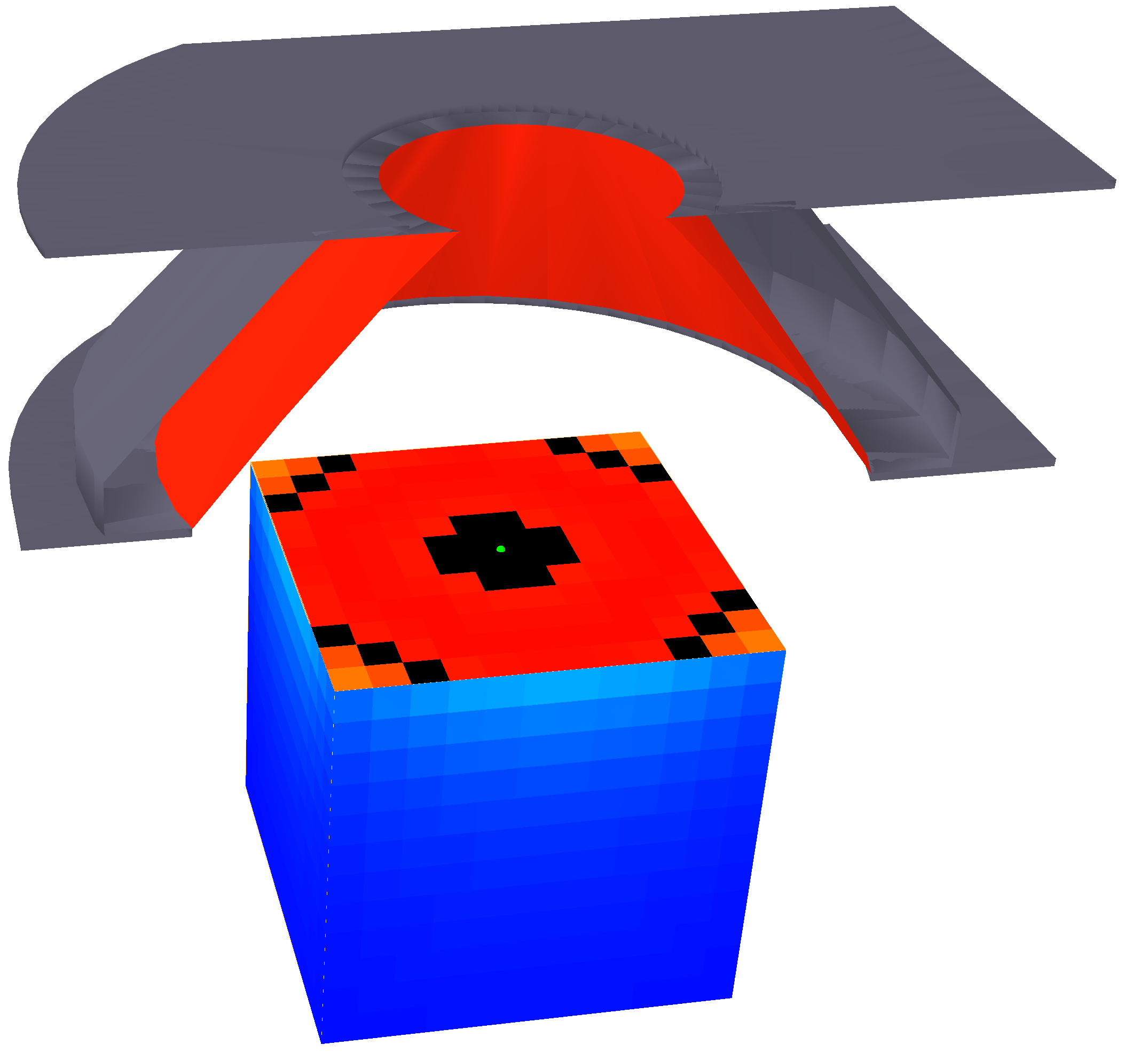
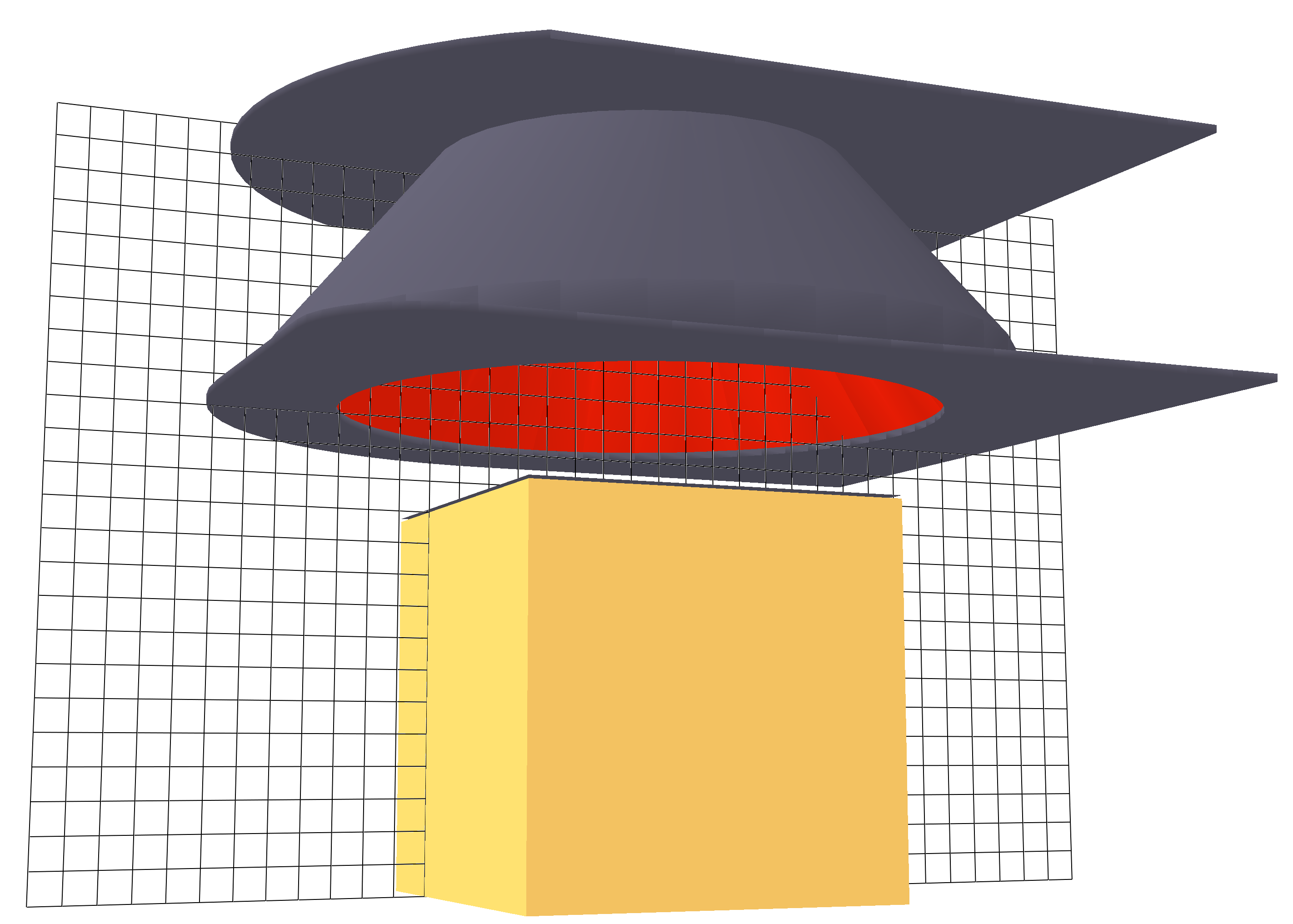
The heater calibration procedure is mimicked in the simulation, to determine the parameters of the boundary condition (SURF) of the heater. A device (DEVC) with the GAUGE HEAT FLUX GAS quantity is located in the centre of where the sample surface is supposed to be during the test. A Python script is used to automatically find an emissivity value for the heater boundary condition that leads to the 65 kW/m² at the device. Refer to the FindTMP_FRONT.py in the ConeRadiationAssessment directory of the data set [28]. The heater temperature is set, based on the temperature reported by Babrauskas, but linearly interpolated between the two enveloping values to get to the desired radiative flux. The simulation includes the gas phase, thus interactions between the radiation and the air are taken into account. The radiative flux is assessed over 20 s, after reaching a quasi-steady state. It is averaged over this time span.

Afterwards, a simulation is conducted in which an obstruction (OBST) is introduced to represent the sample and its holder. There is a distance of 25 mm between the sample surface and the bottom of the cone heater assembly. From the top boundary of the obstruction the radiative heat flux is recorded (GAUGE HEAT FLUX). Per cell, it is averaged over 20 s after reaching a quasi-steady state, same as in the previous step.

Appendix B Computational Domain Layouts

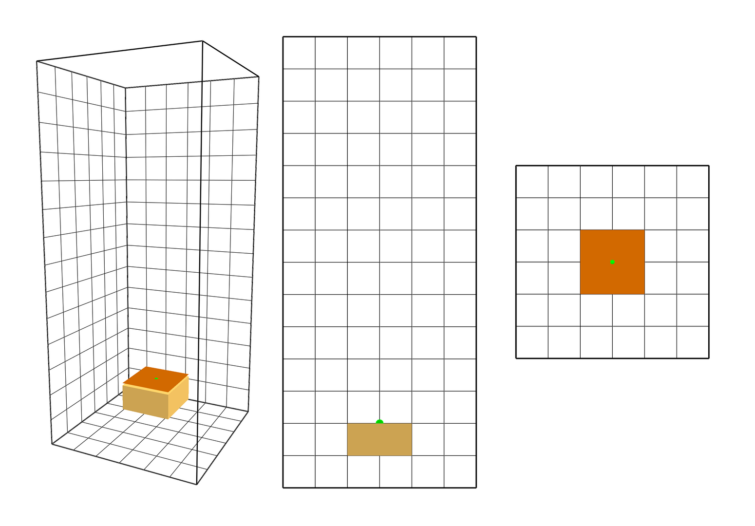
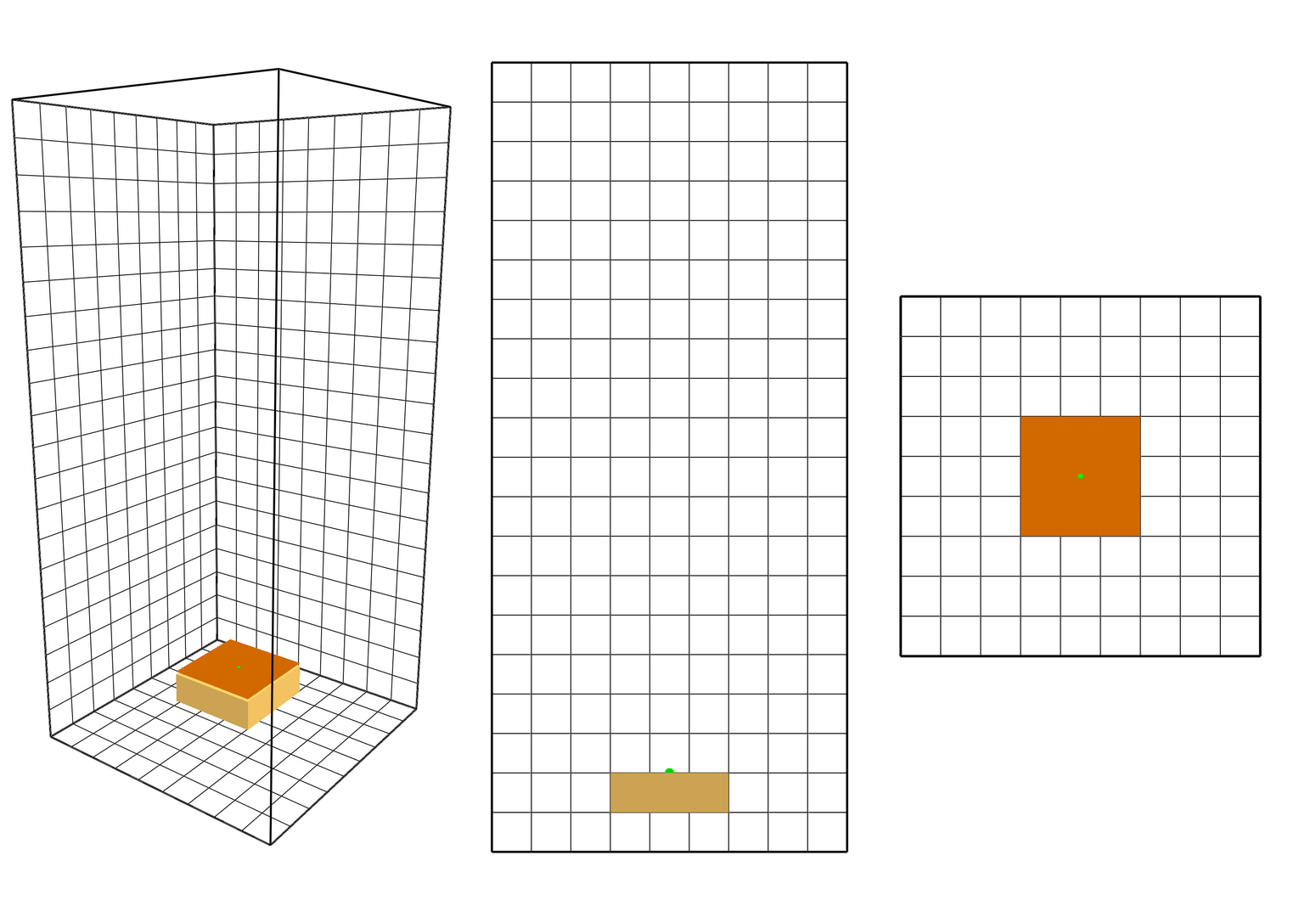
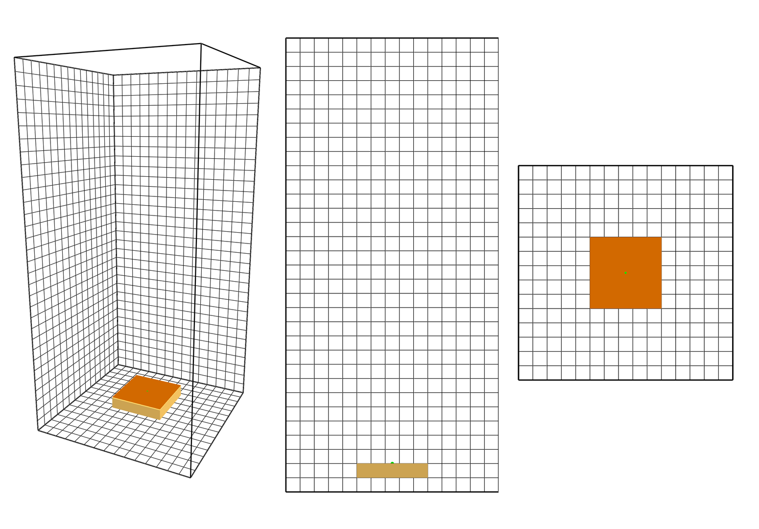
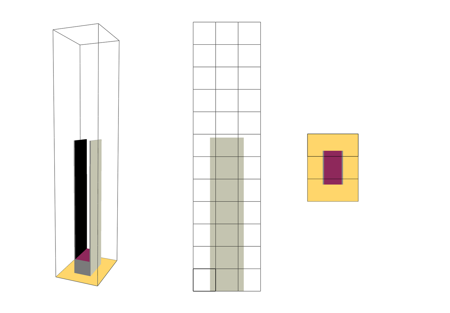
Appendix C Complex Chemistry

During the simple chemistry FDS calculates the stoichiometry itself and provides the results in the CHID.out file. This, however, only works if FDS is used regularly, meaning not with TGA_ANALYSIS. A Python script was designed that automatically finds the recent best parameter set (lowest RMSE, see section 2.2) from the micro-scale IMP and creates a new FDS input file to generate a respective CHID.out file. After manual execution of this simulation the script can extract the needed stoichiometry information from the CHID.out file, build the appropriate input lines and write them to a new FDS input file. These steps are handled in the GetChemicalReaction.ipynb notebook, which can be found in the data repository [28]. To ensure consistency, the repetition information of the best parameter set is written to the respective FDS input files as well. For the parallel panel simulations this information can be copied over manually.

Appendix D Mass Losses and Flame Heights

An example parameter set is used to demonstrate the different mass loss rates and energy release. The cases "Cone 01" to "Cone 03" in figures LABEL:fig:FlameHeight_MassLoss_Solid, LABEL:fig:FlameHeight_MassLoss_Gas and 27 all use the same pyrolysis scheme. "Cone 01" and "Cone 02" use only methane as surrogate fuel. For "Cone 01" the heat of combustion in the material definition is set to 25 MJ/kg, which is about half of the value of pure methane. No heat of combustion value is provided for "Cone 02", thus it is the predefined value of 50 MJ/kg of methane. "Cone 03" uses a surrogate fuel gas mixture that consists of 26 volume percent of carbon dioxide and 74 volume percent of methane. This leads to roughly the same average heat of combustion than the 25 MJ/kg of "Cone 01". Also, the radiative fraction of the gas mixture was set to 0.20 to match the value of pure methane. Again, no HOC value is provided in the material definition, thus the released mass in the solid is transported directly to the gas domain. This highlights the distinction between the solid and gas phase side of the FDS simulation. FDS uses the heat of combustion parameter provided in the material definition to scale the mass of fuel that is introduced into the gas domain. Figure LABEL:fig:FlameHeight_MassLoss_Solid shows the mass loss in the solid. All three cases experience a very similar development. In figure LABEL:fig:FlameHeight_MassLoss_Gas it can be observed that the mass introduced into the gas domain is about half for "Cone 01" compared to the others, due to the scaling of the HOC. Consequently, figure 27 shows about double the energy release for case "Cone 02" than the others.

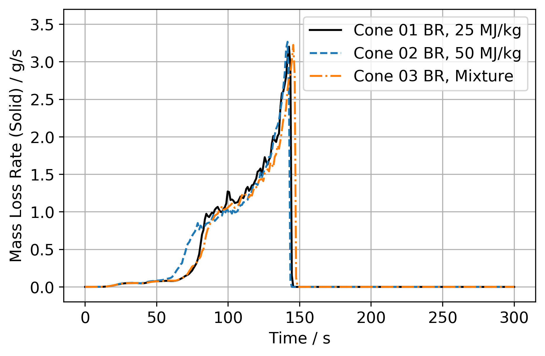
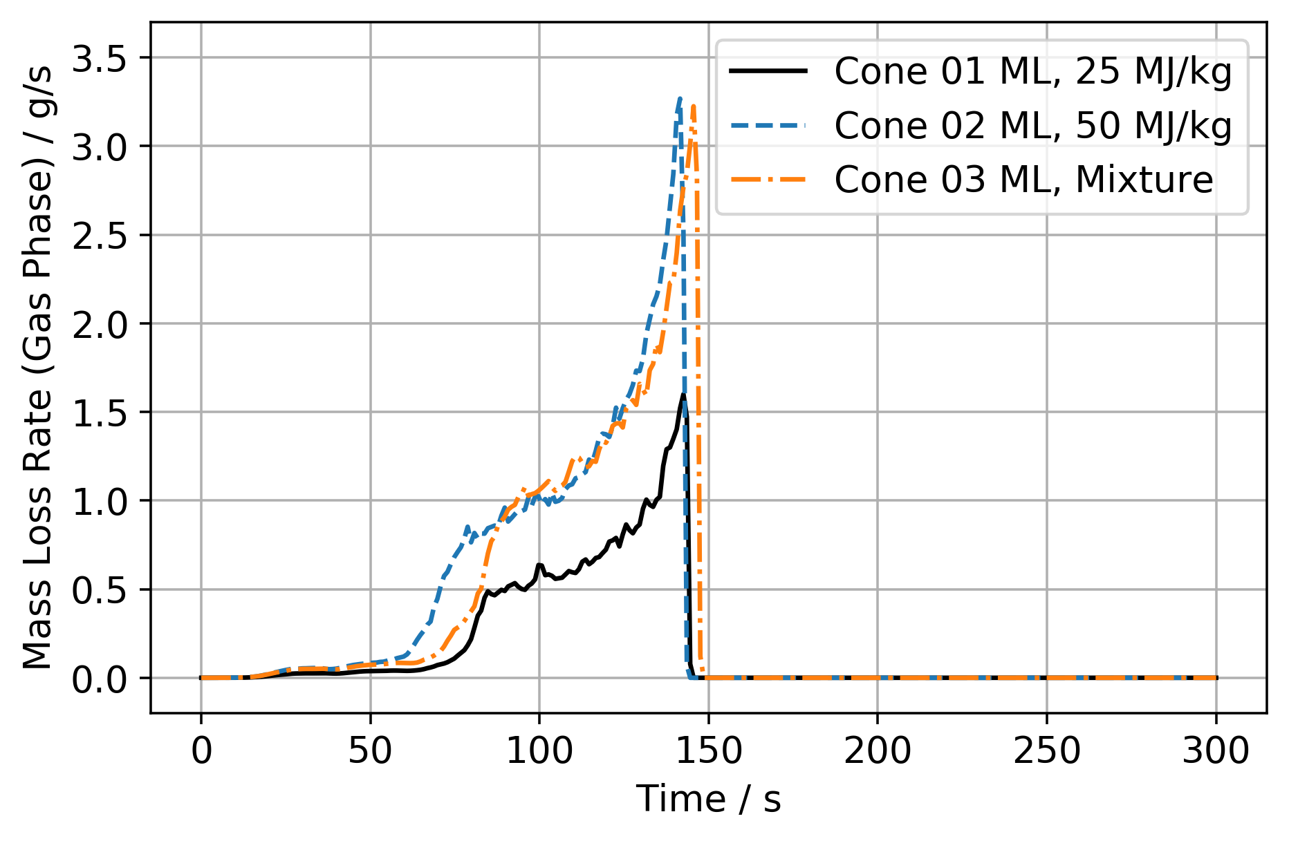
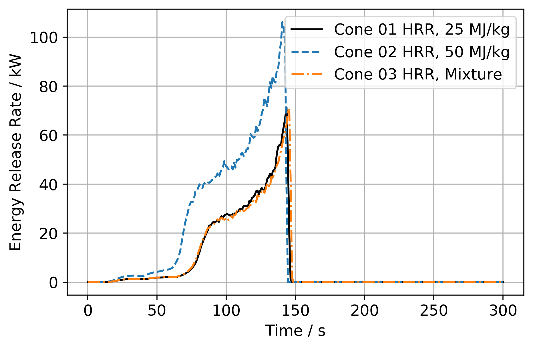
The different surrogate fuel strategies from above, "Cone 01" and "Cone 03", lead also to different flames. Two simulations are conducted with a constant mass release (HRRPUA), shown in figure LABEL:fig:FlameHeight_MassLoss to mimic both setups. Gas temperatures are recorded on the vertical centre line of the flame and averaged over the second half of the simulation (30 s). This leads to differences in the flame structure as shown in figure LABEL:fig:FlameHeight_Temperatures. No claim is made here as to which one is more "realistic", just the difference pointed out.

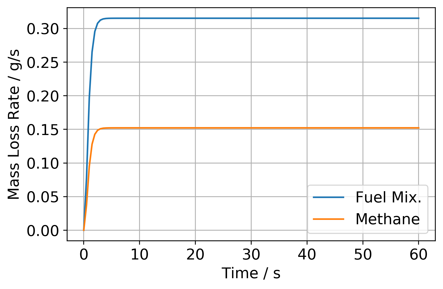
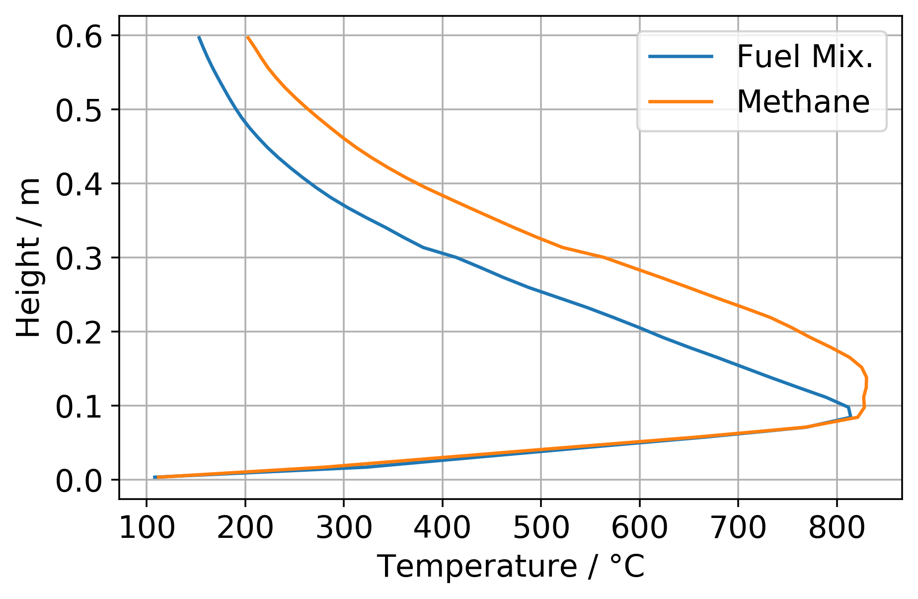
Appendix E Example Limit Adjustments

During the IMP individual parameters can get stuck at their limits. Figure 29 shows an example of this. During the initial limit definition (L0) the pyrolysis range parameter got stuck at its upper limit. Another IMP run was set up, with an expanded range (L1). Note: only the upper limit was adjusted and the lower limit was kept at its original value. Thus, the sampling space only grows larger over multiple adjustments. In the beginning, both developments are different, because not only this parameters limits are adjusted for this new run, but also for others that were stuck.

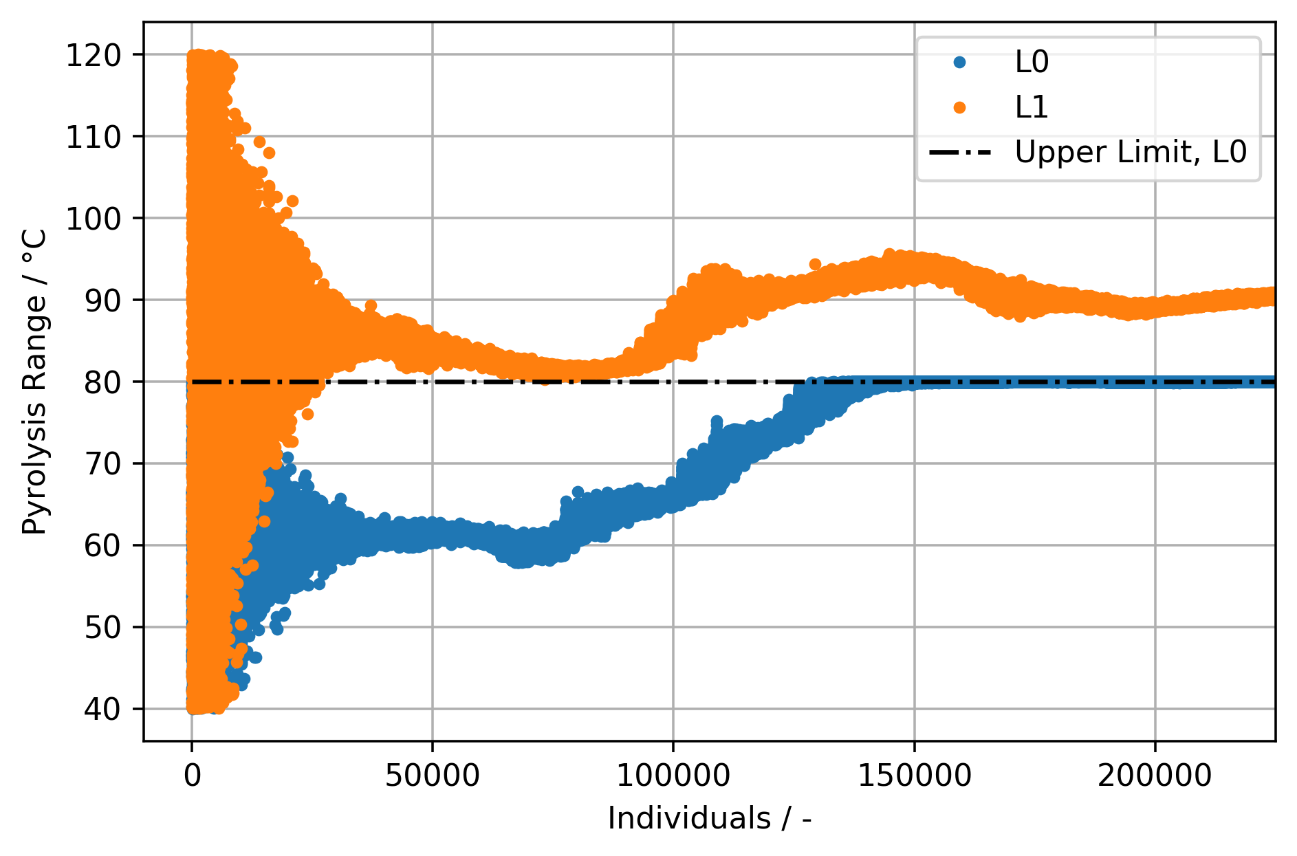
Appendix F Micro-Scale Tests

Data sets from the micro-scale tests. NIST reported that the equipment for the TGA was a Netzsch F1 Jupiter and a FAA microscale combustion calorimeter for the MCC, Sandia used a Netzsch F3 Jupiter [7].

The TGA experiments by NIST were conducted in nitrogen atmosphere. For the MCC experiments the pyrolysis chamber was fed with nitrogen and oxygen was mixed into the effluents before entering the combustion chamber. The TGA experiments by Sandia were conducted in argon atmosphere.

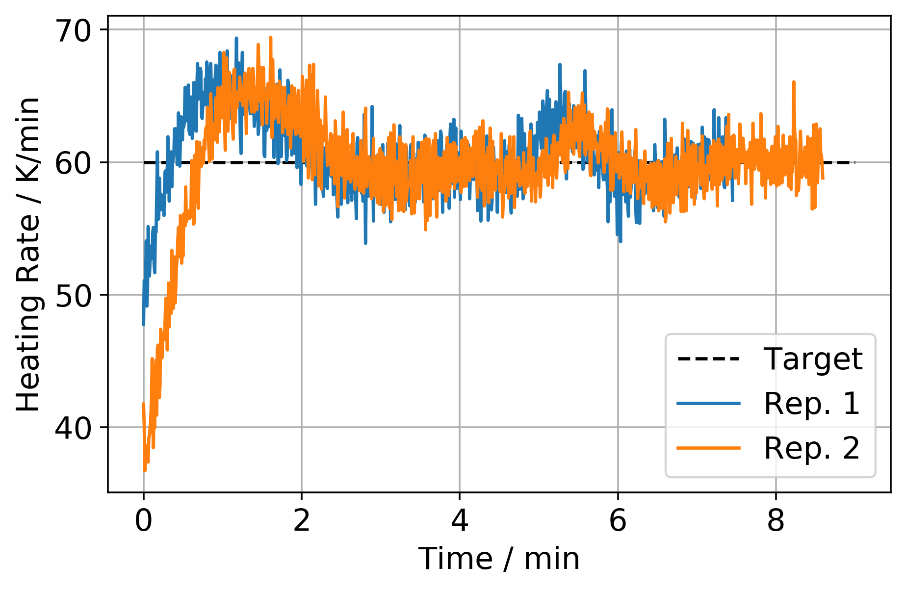
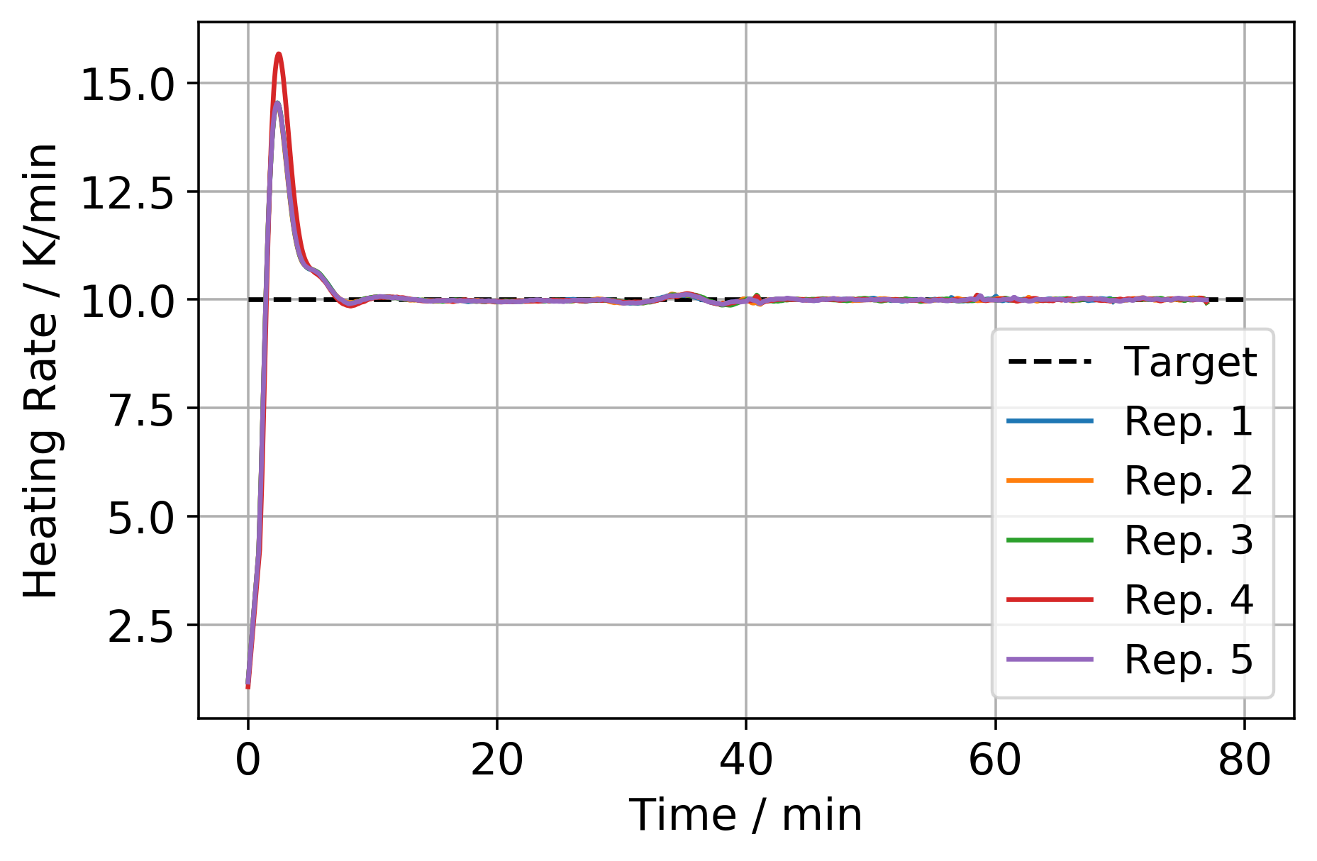
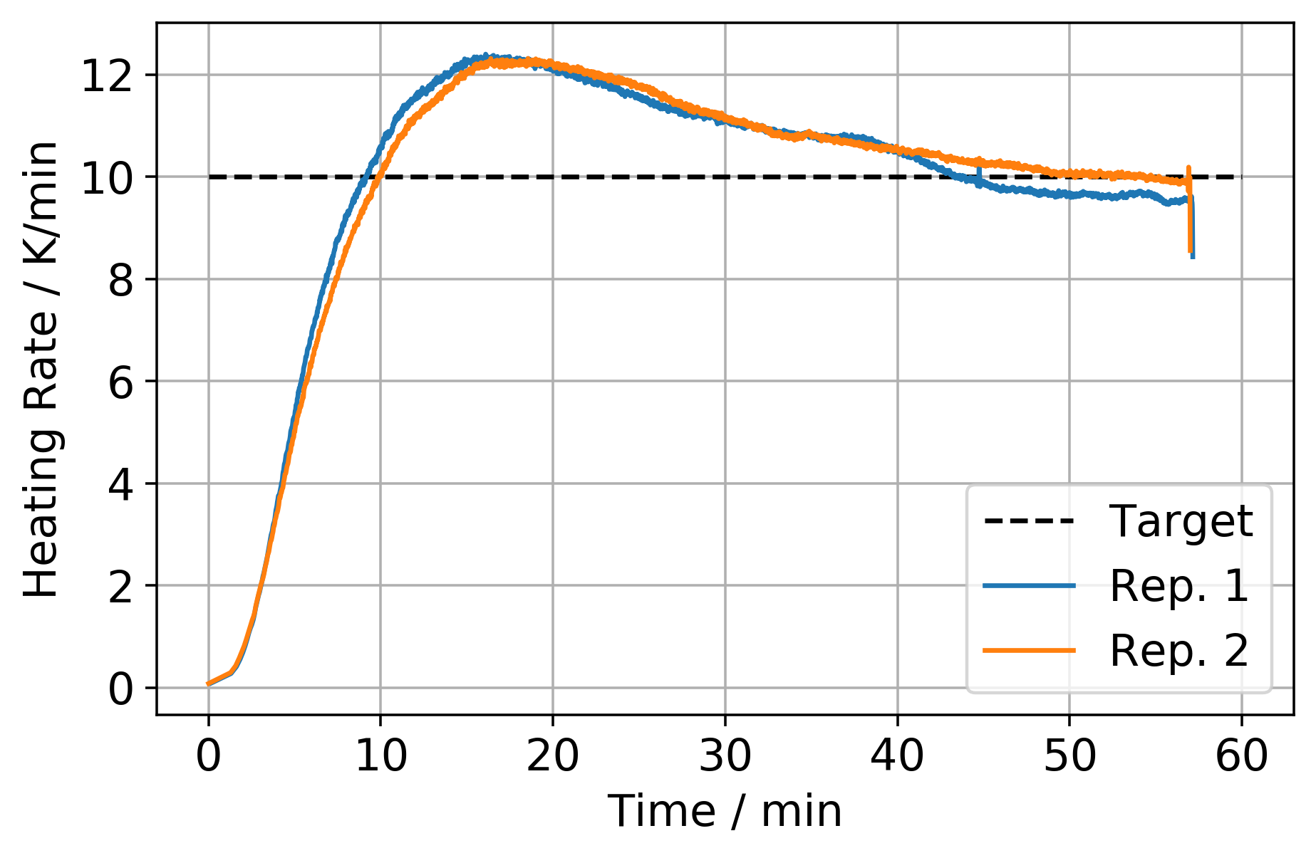
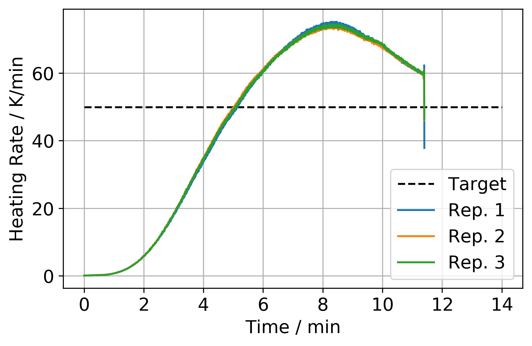
Appendix G Simple Cone Calorimeter Simulation Results

G.1 IMP Fitness Development

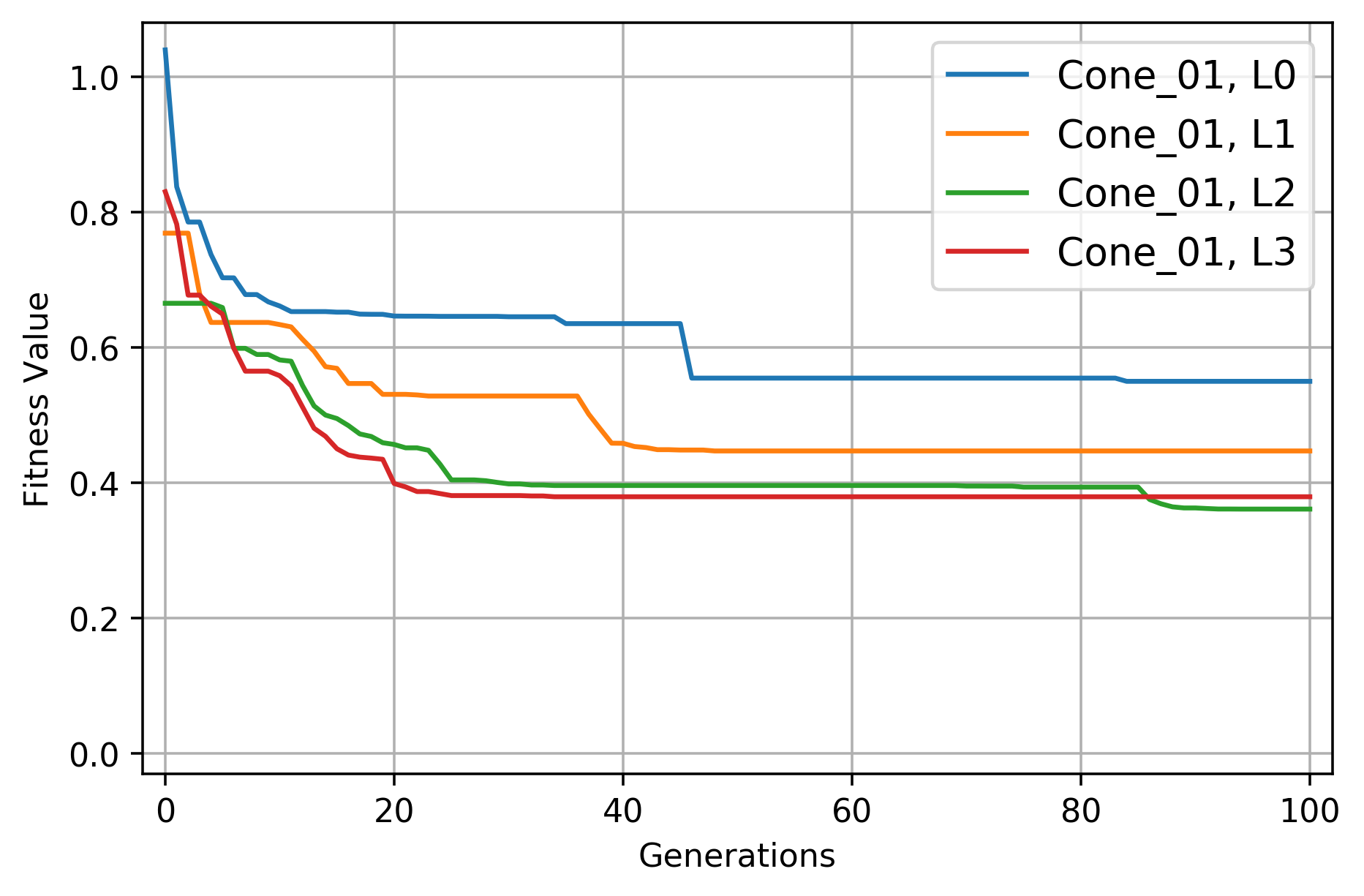
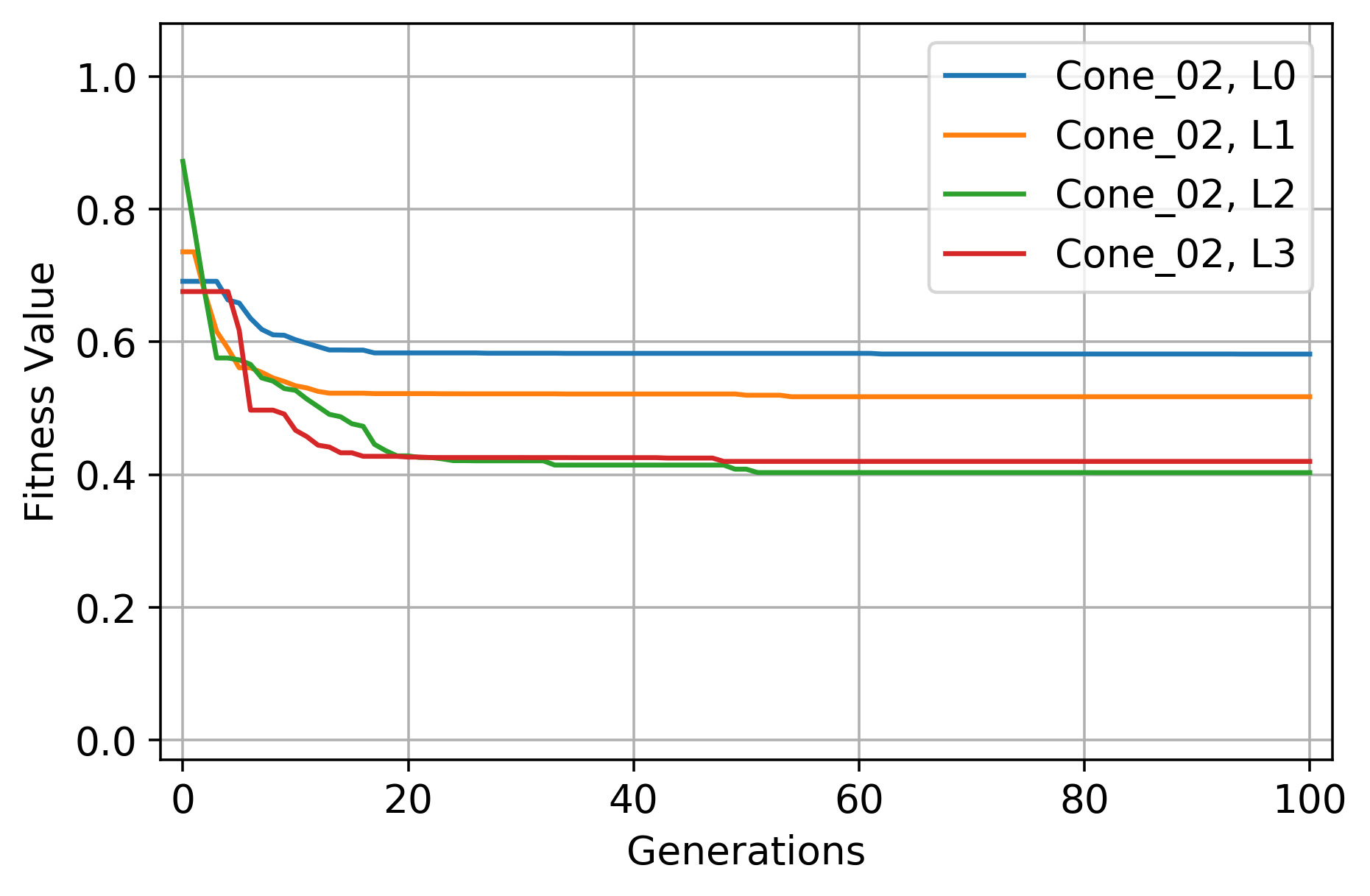
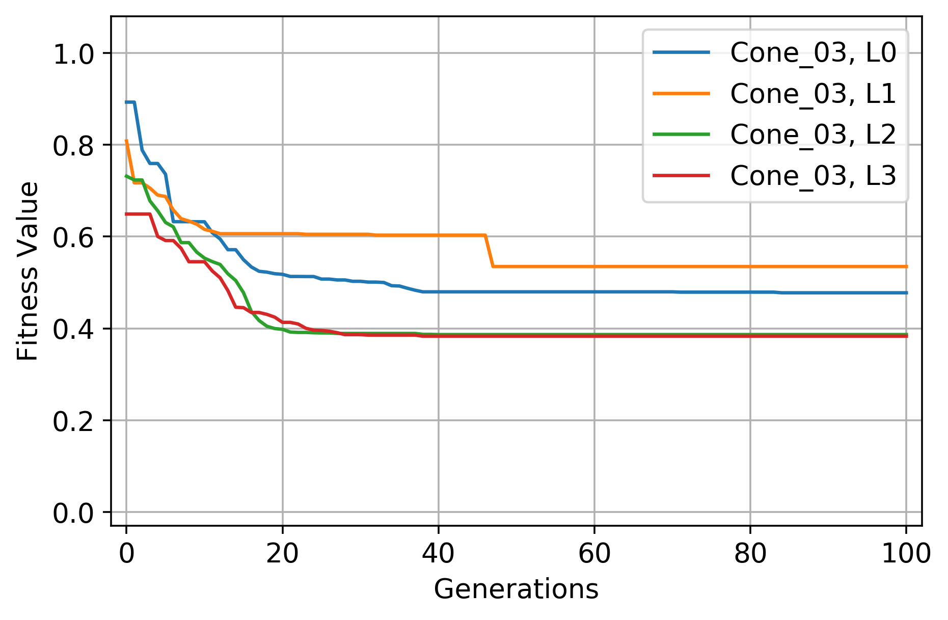
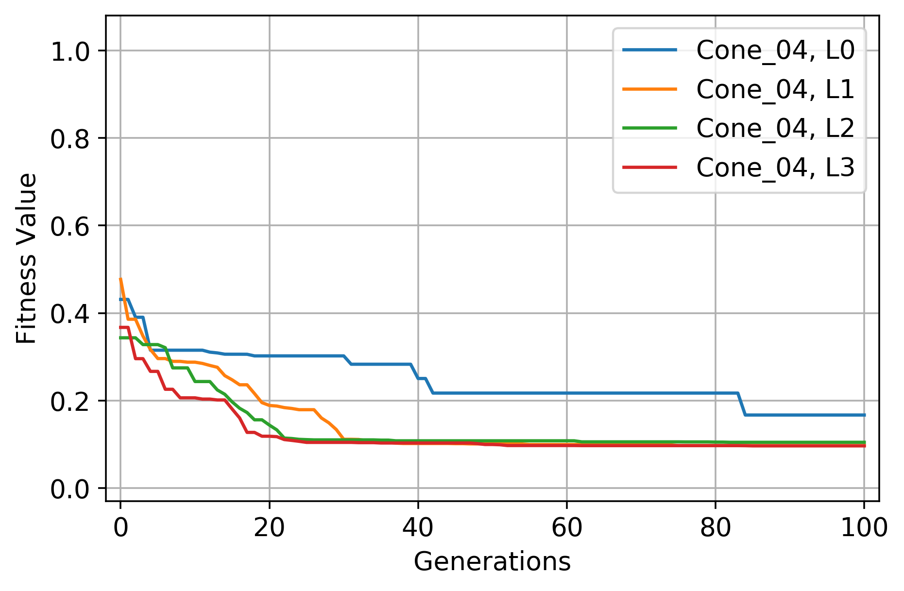
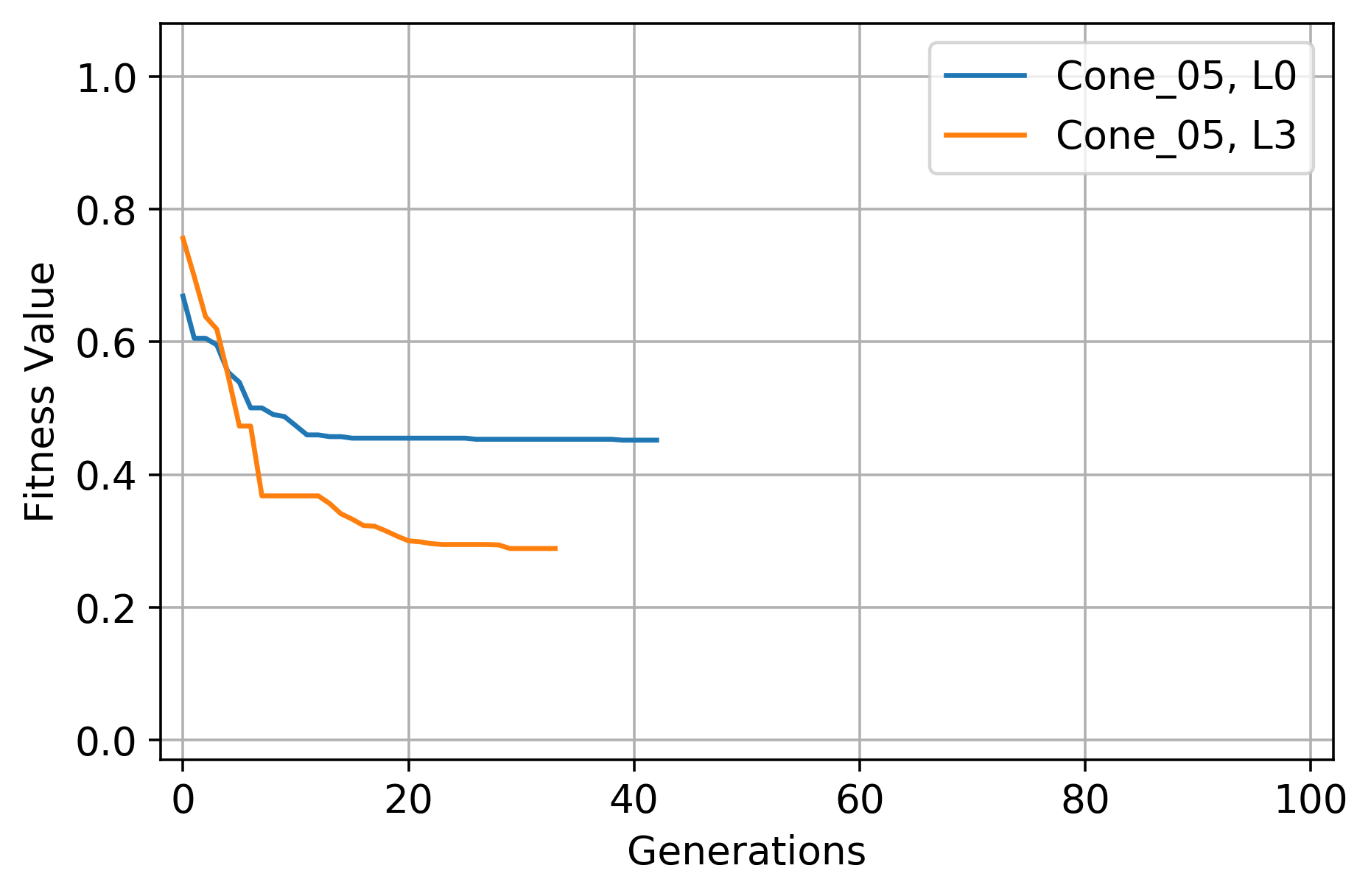
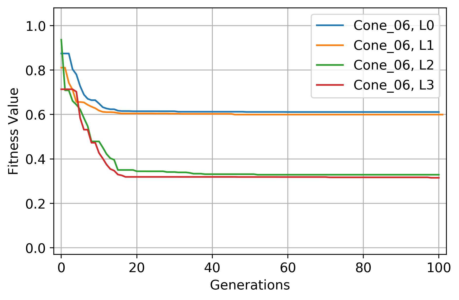
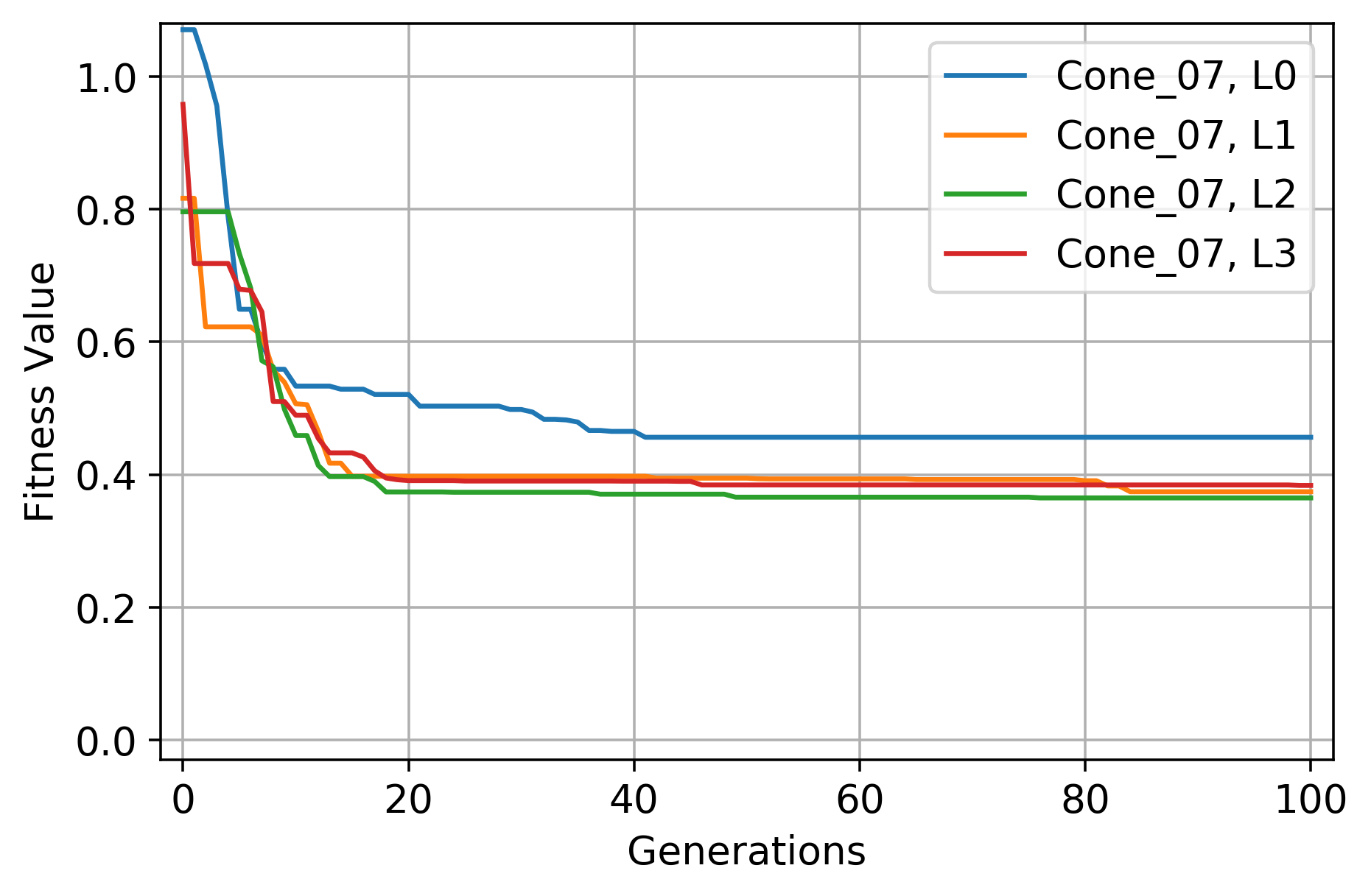
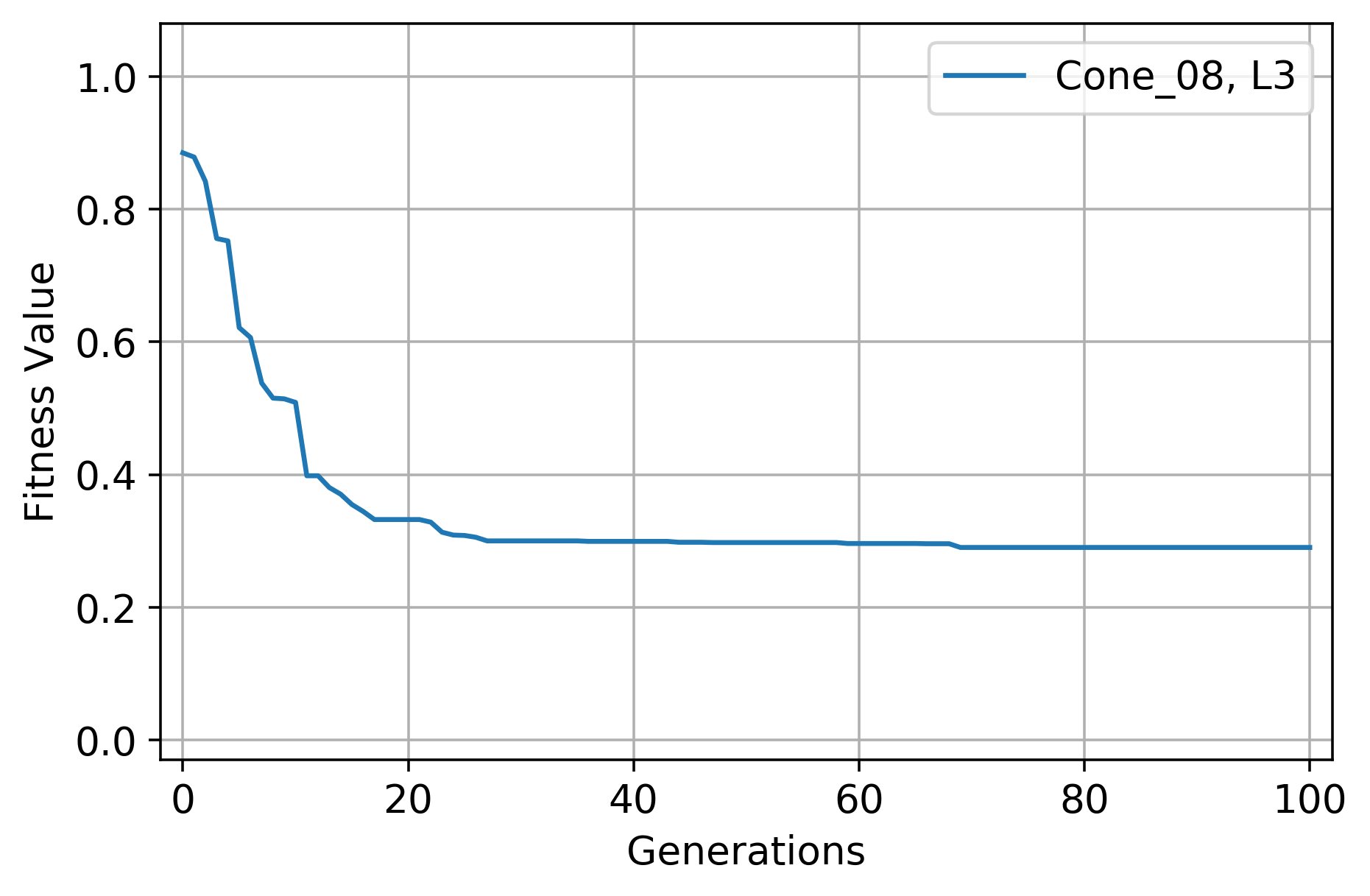
G.2 Energy Release Rates

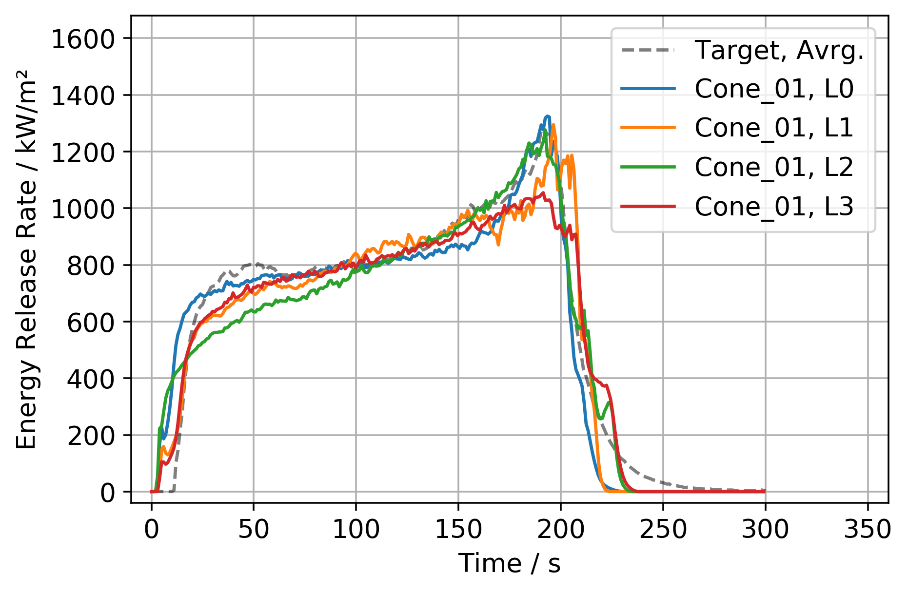
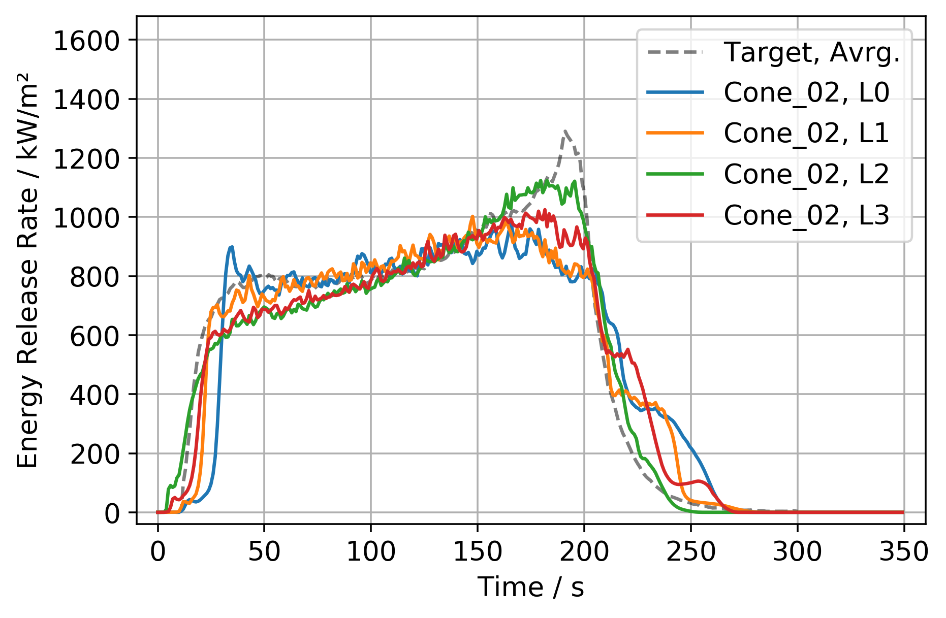
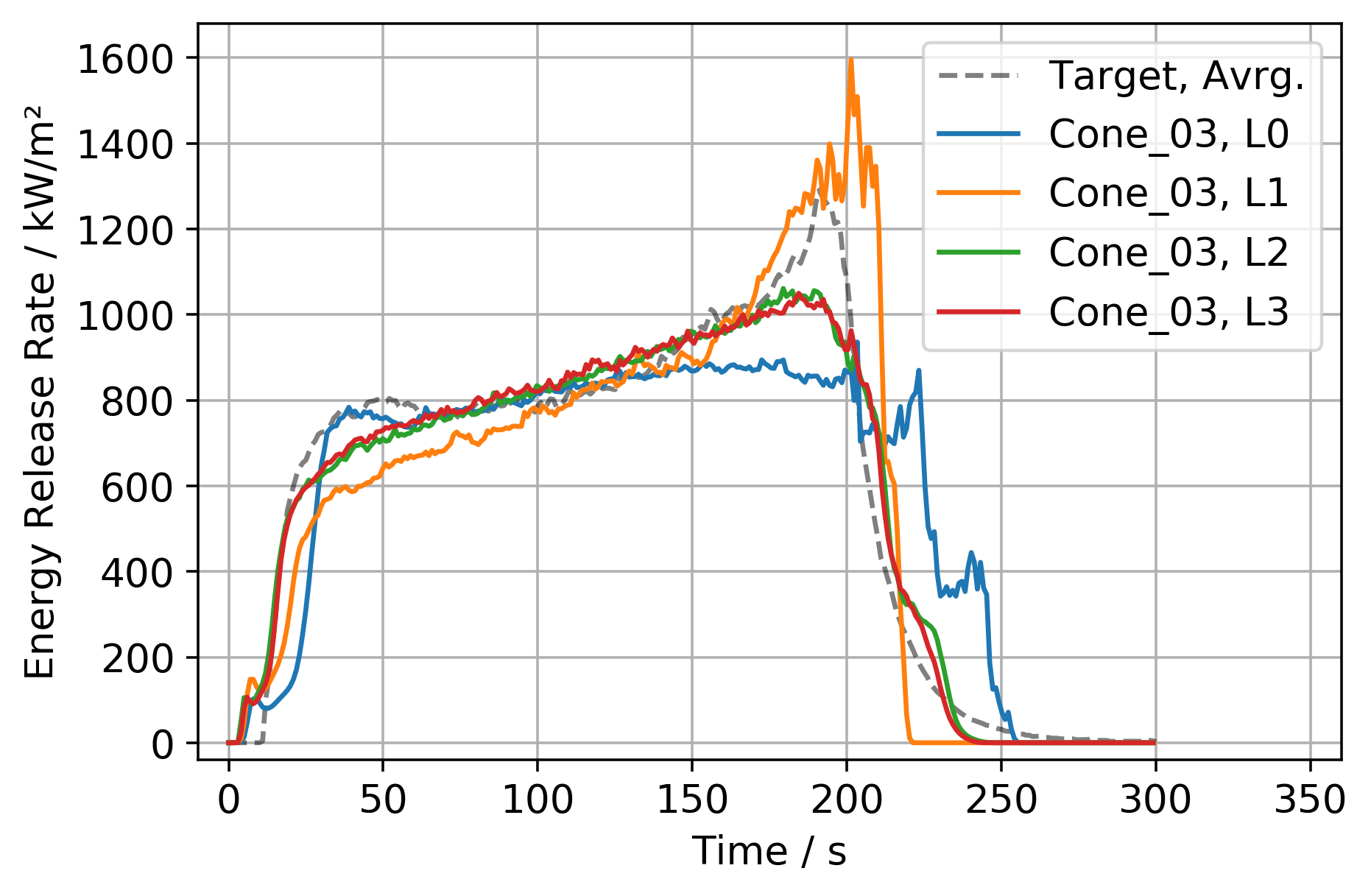
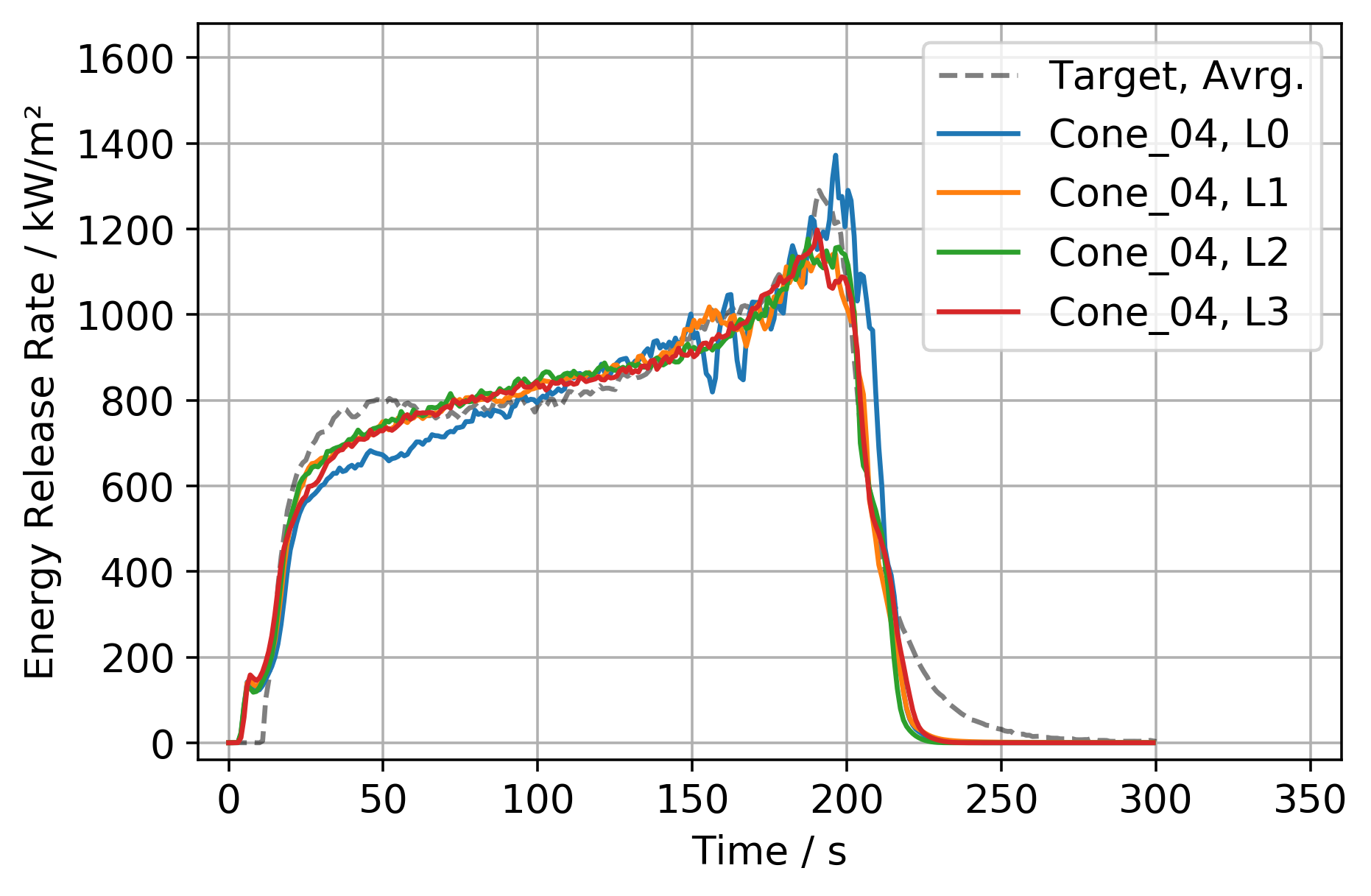
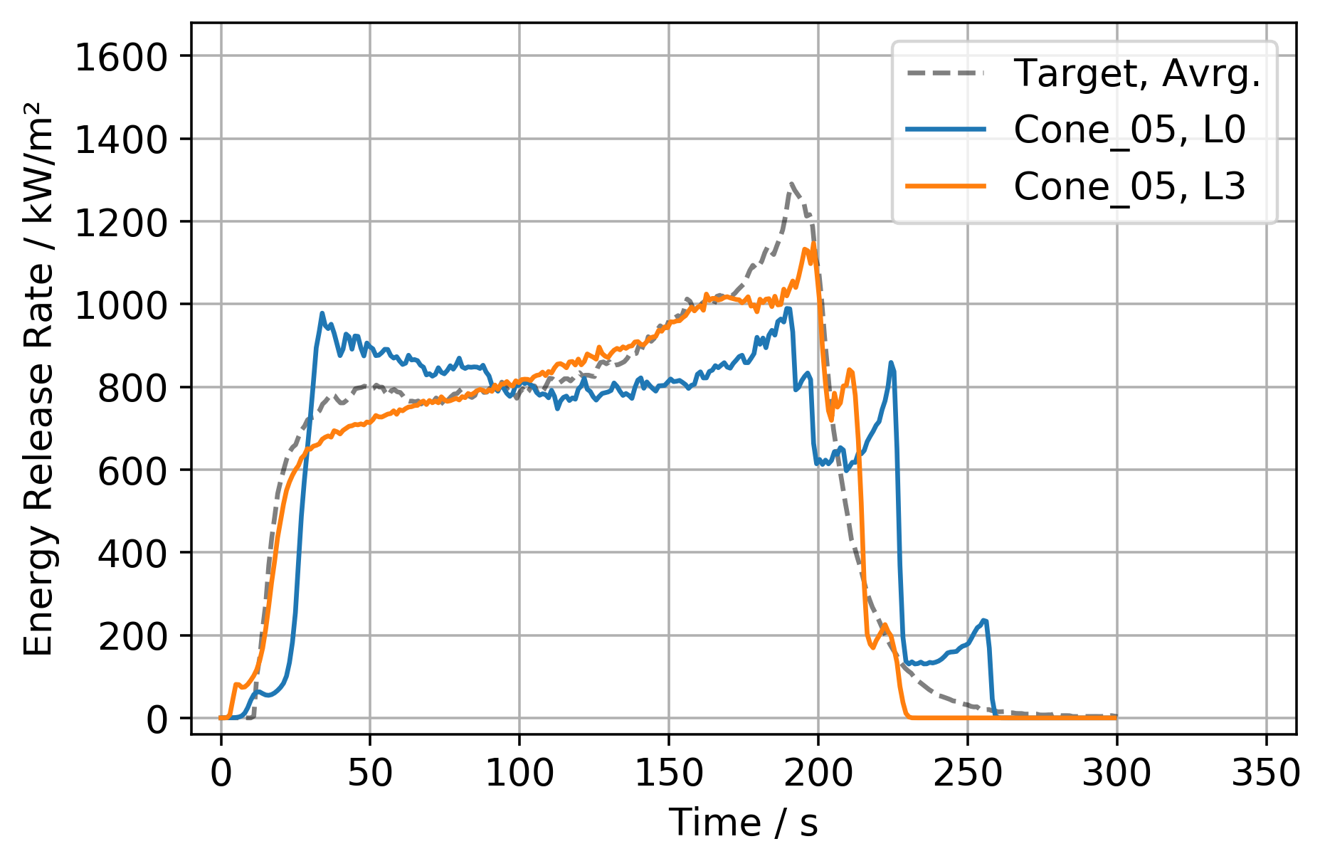
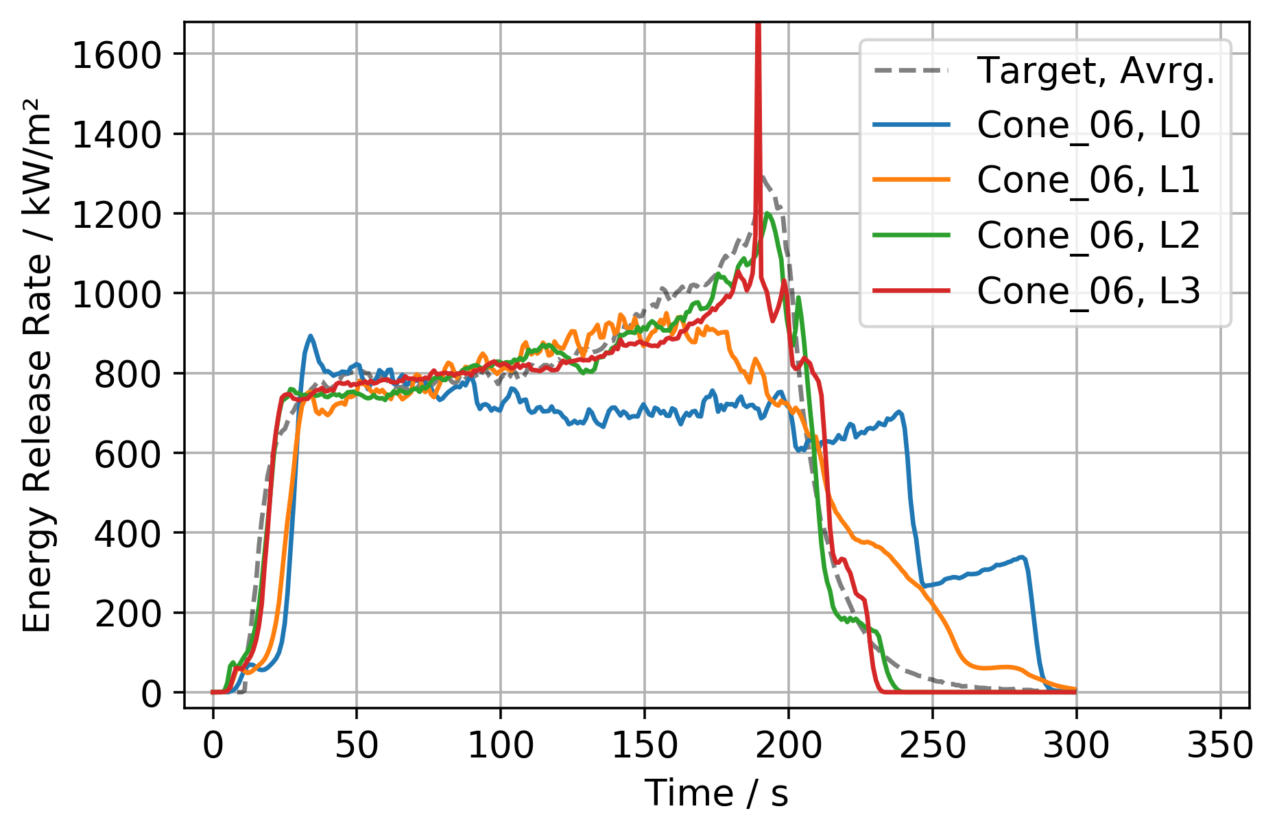
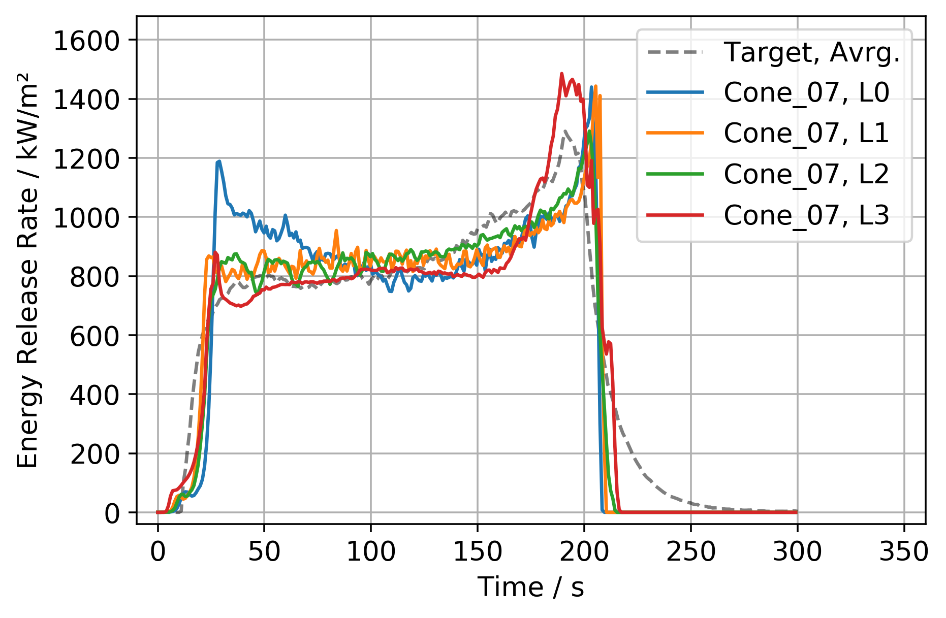
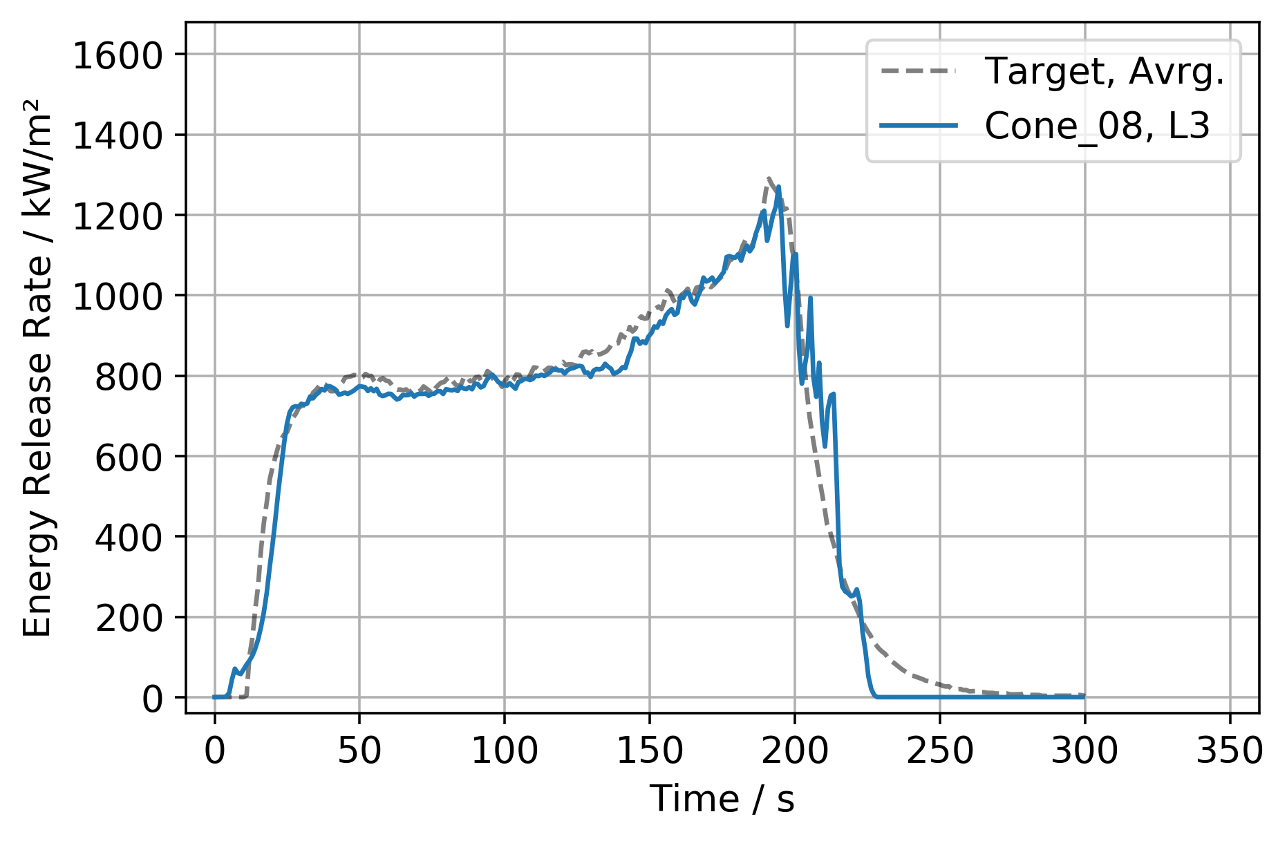
G.3 Back Side Temperatures

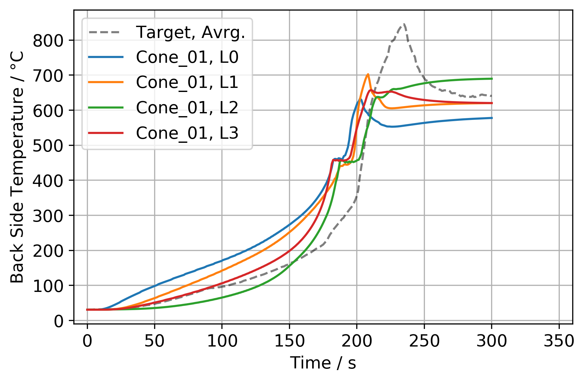
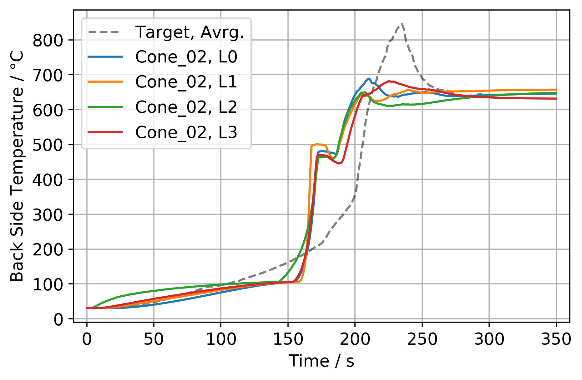
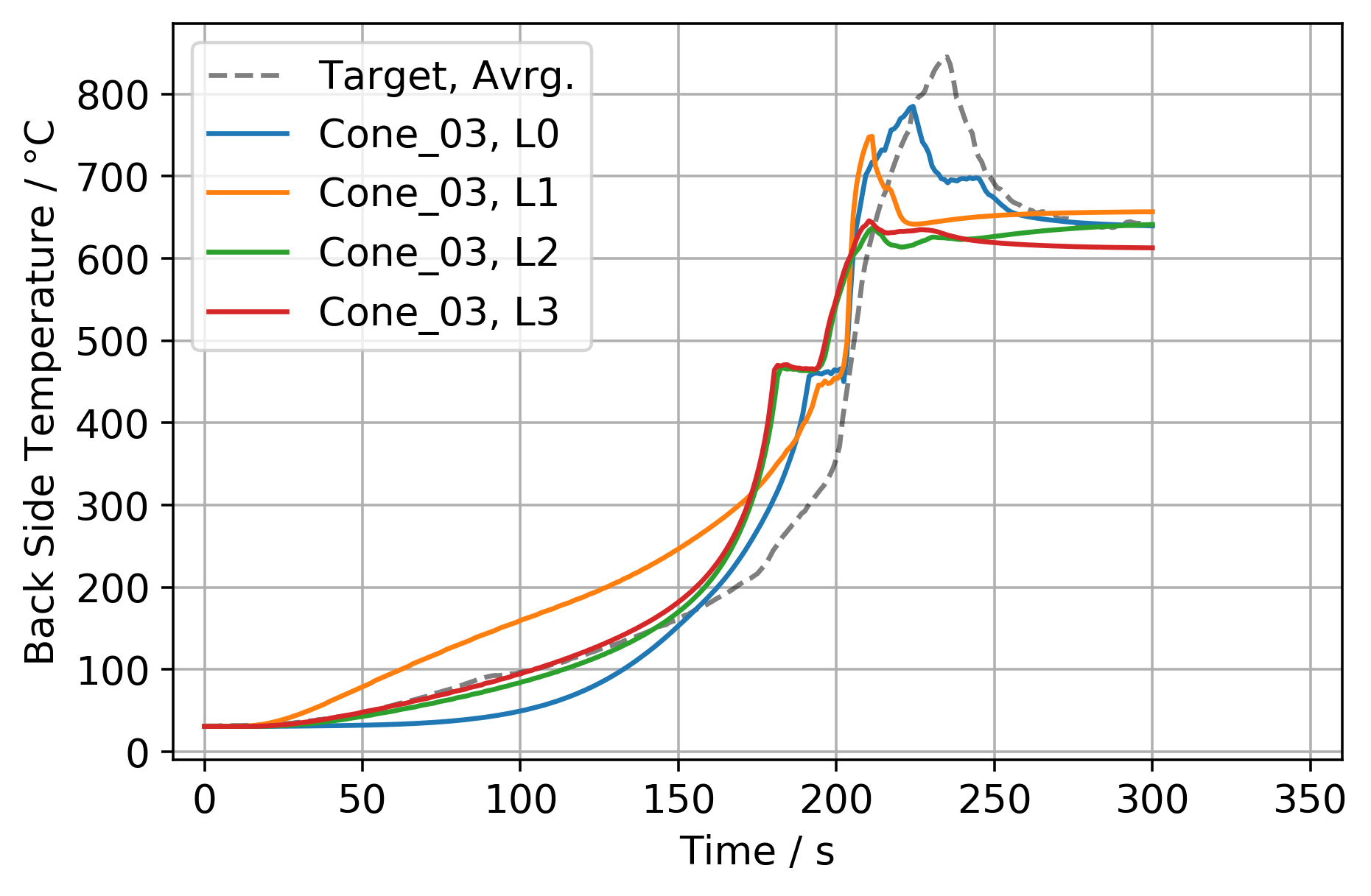
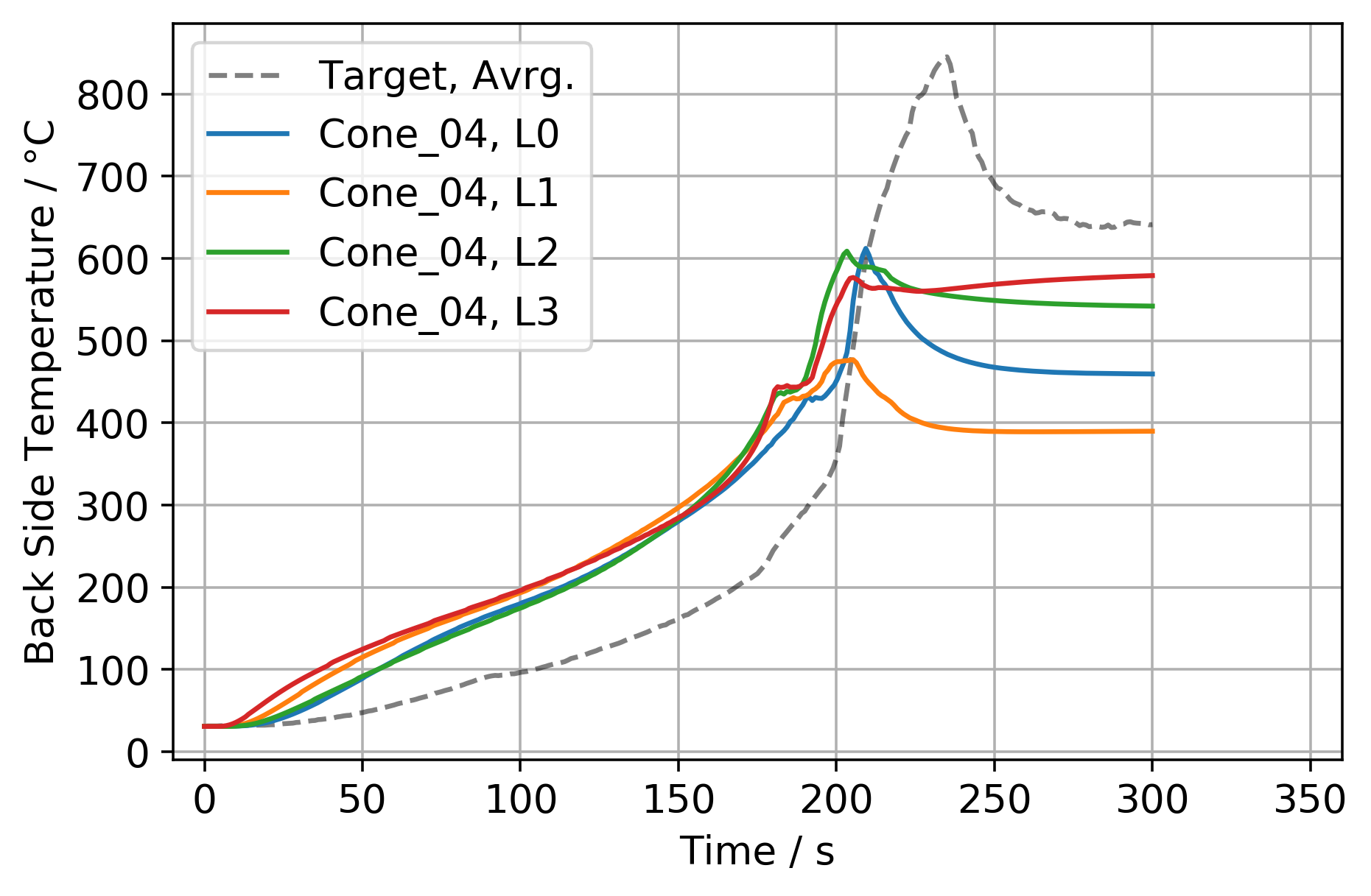
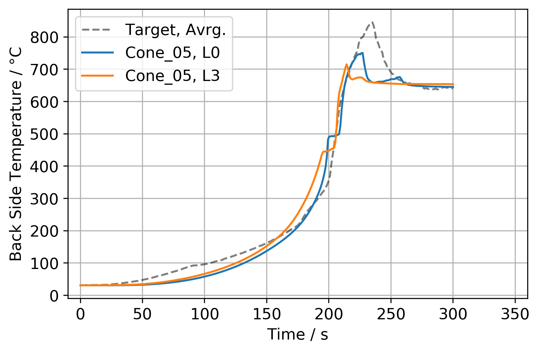
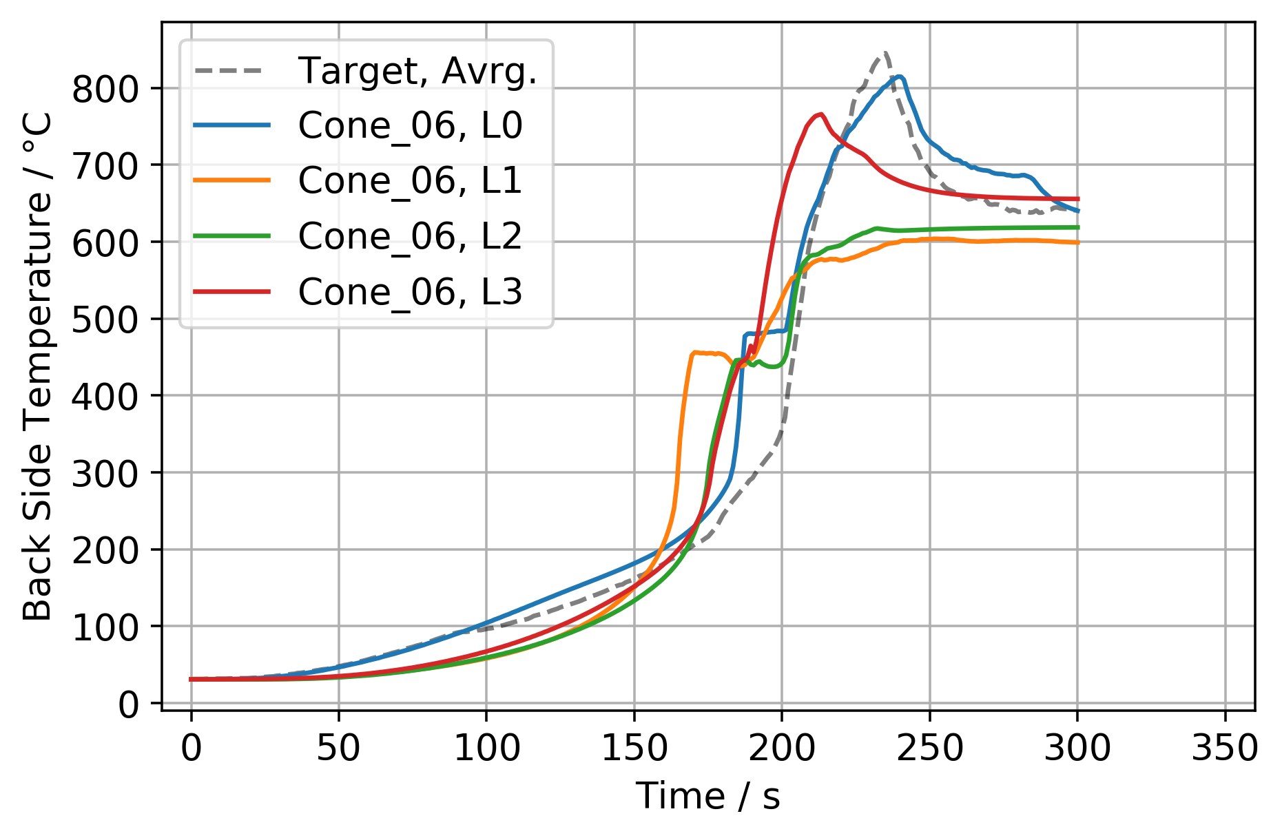
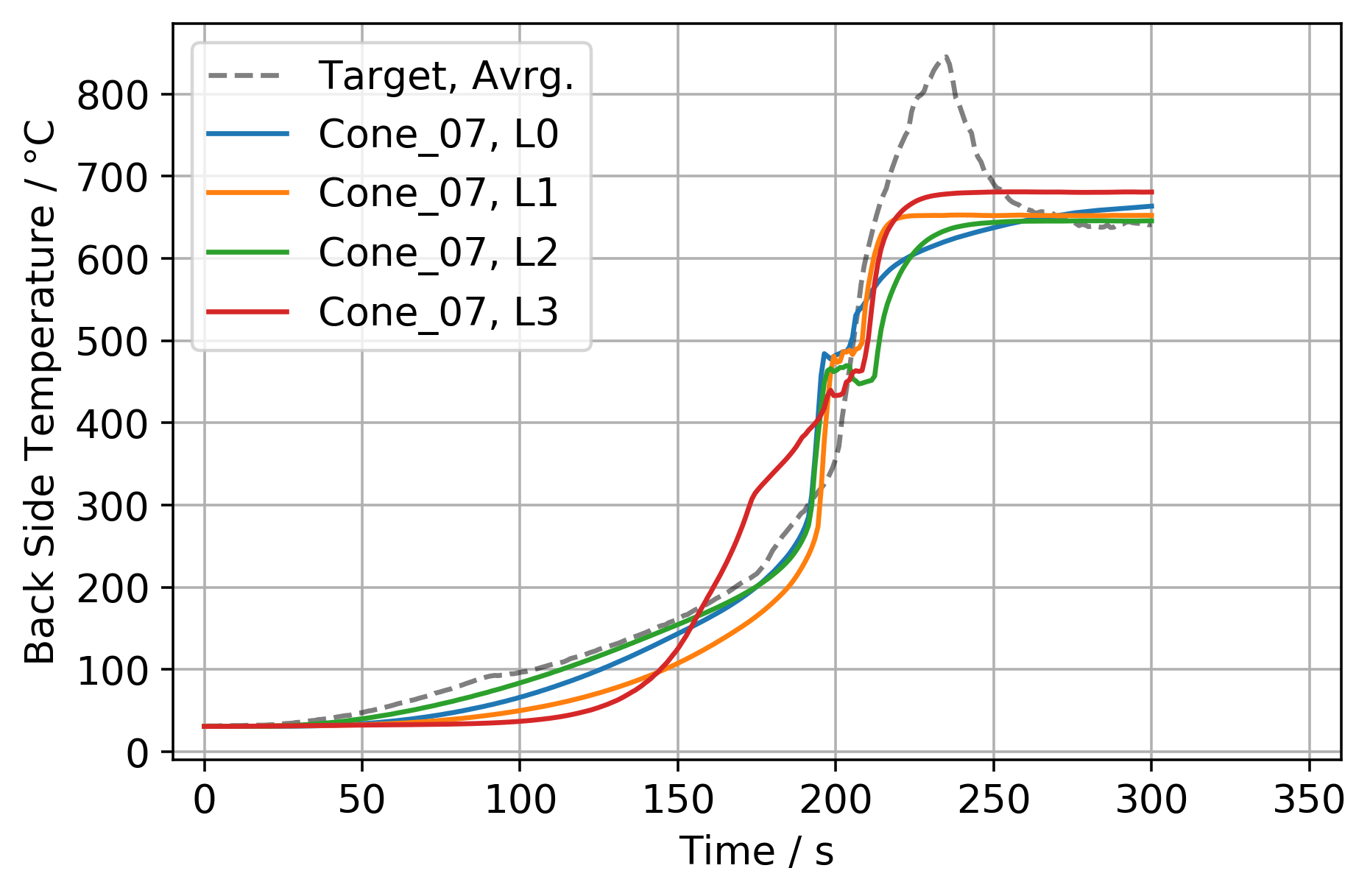
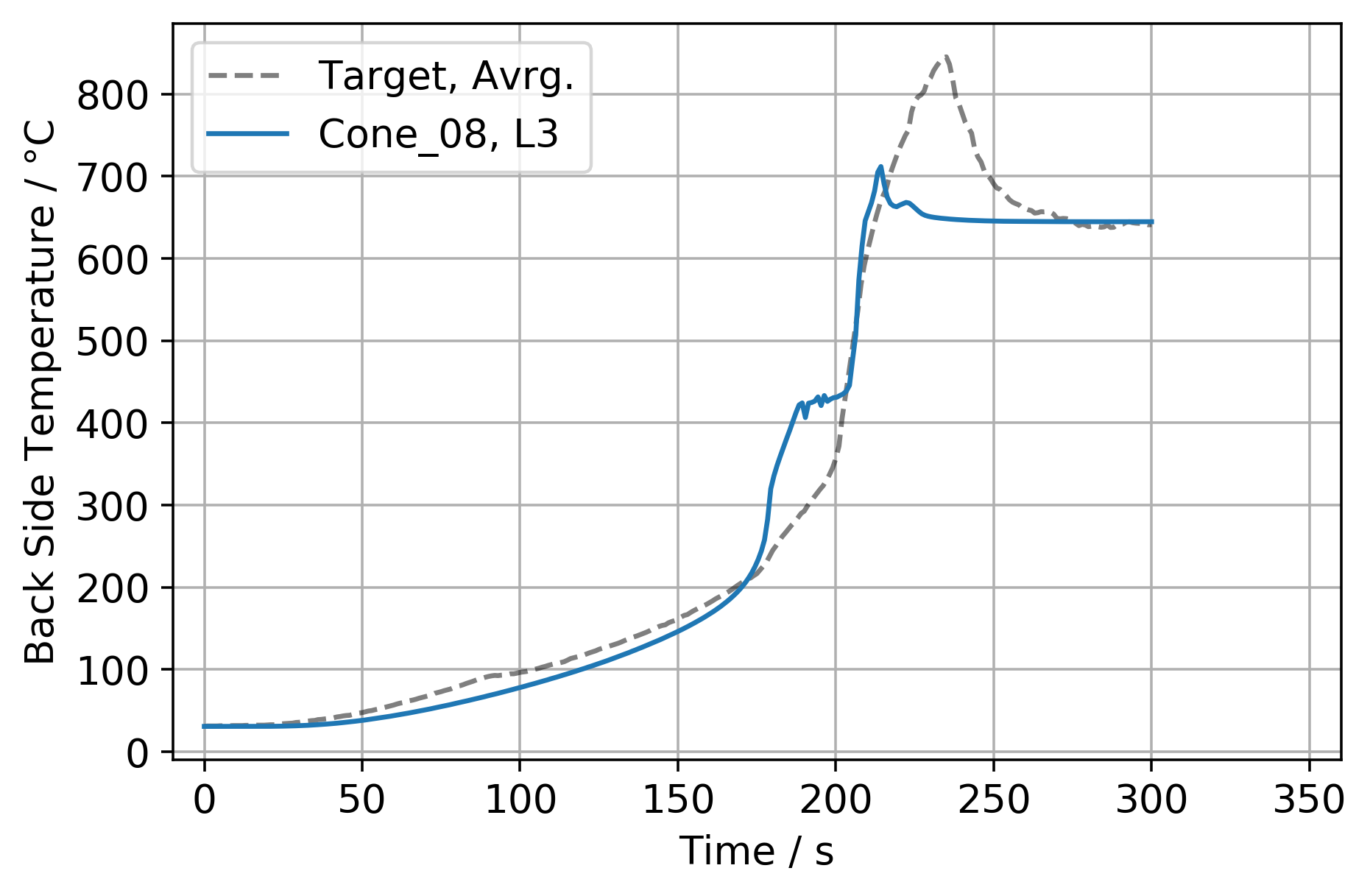
G.4 Thermal Conductivity

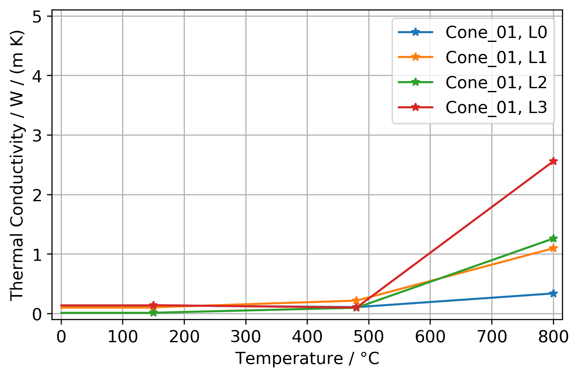
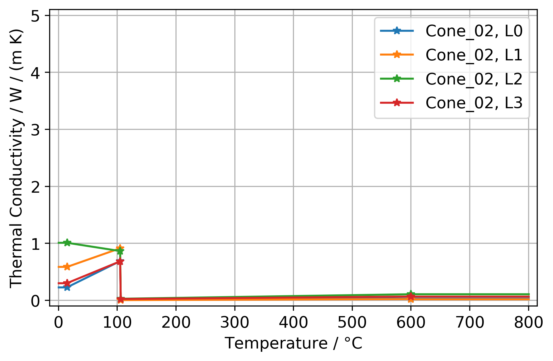
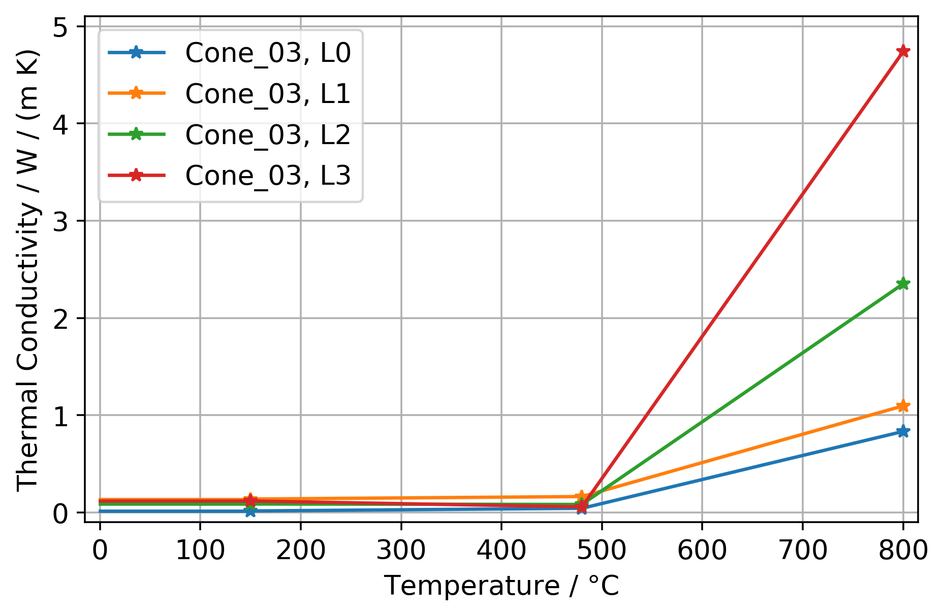
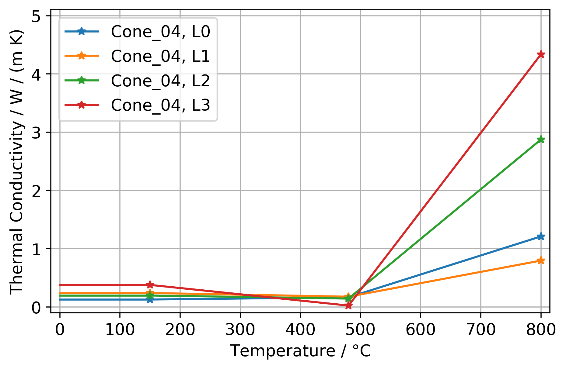
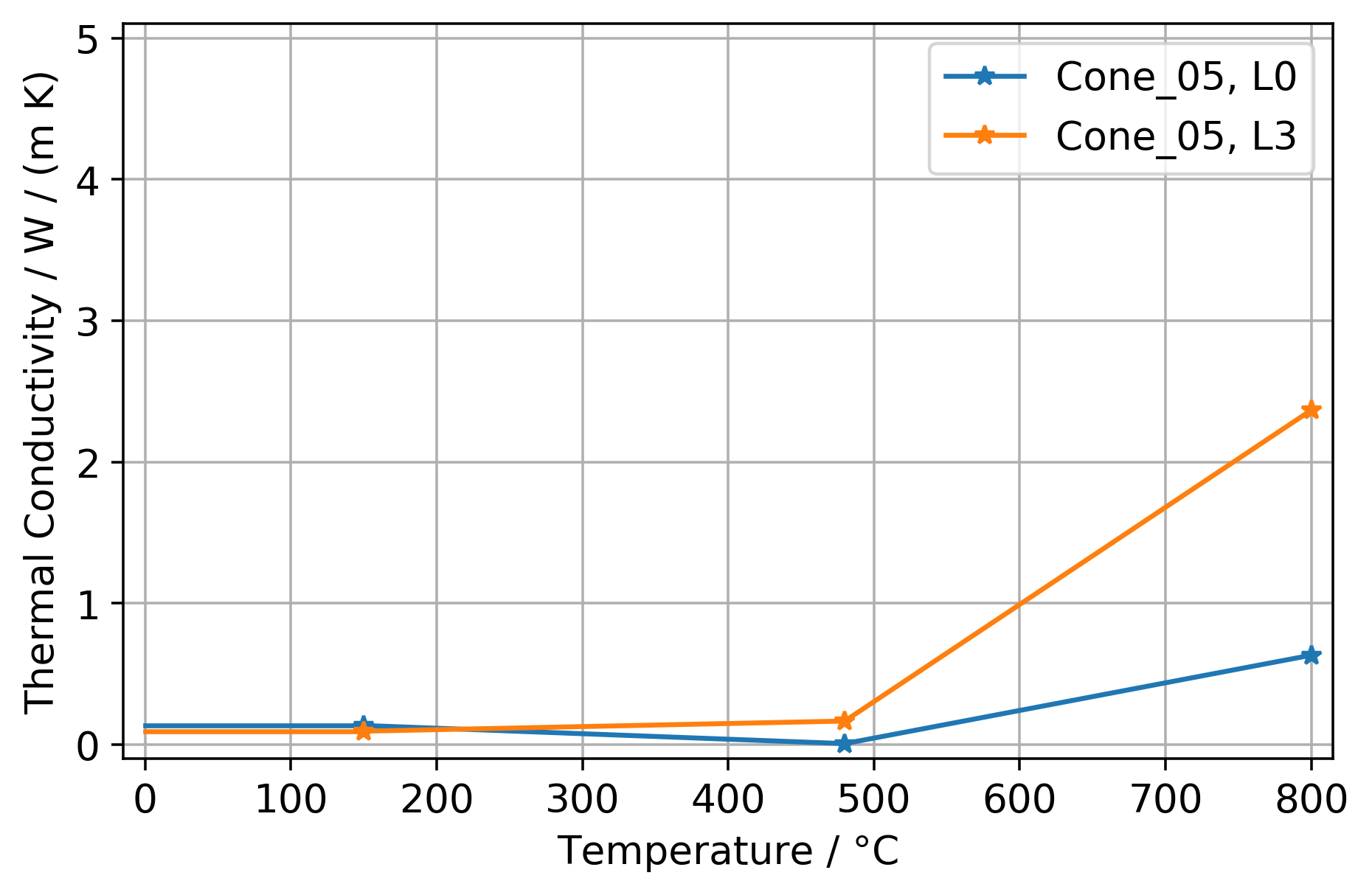
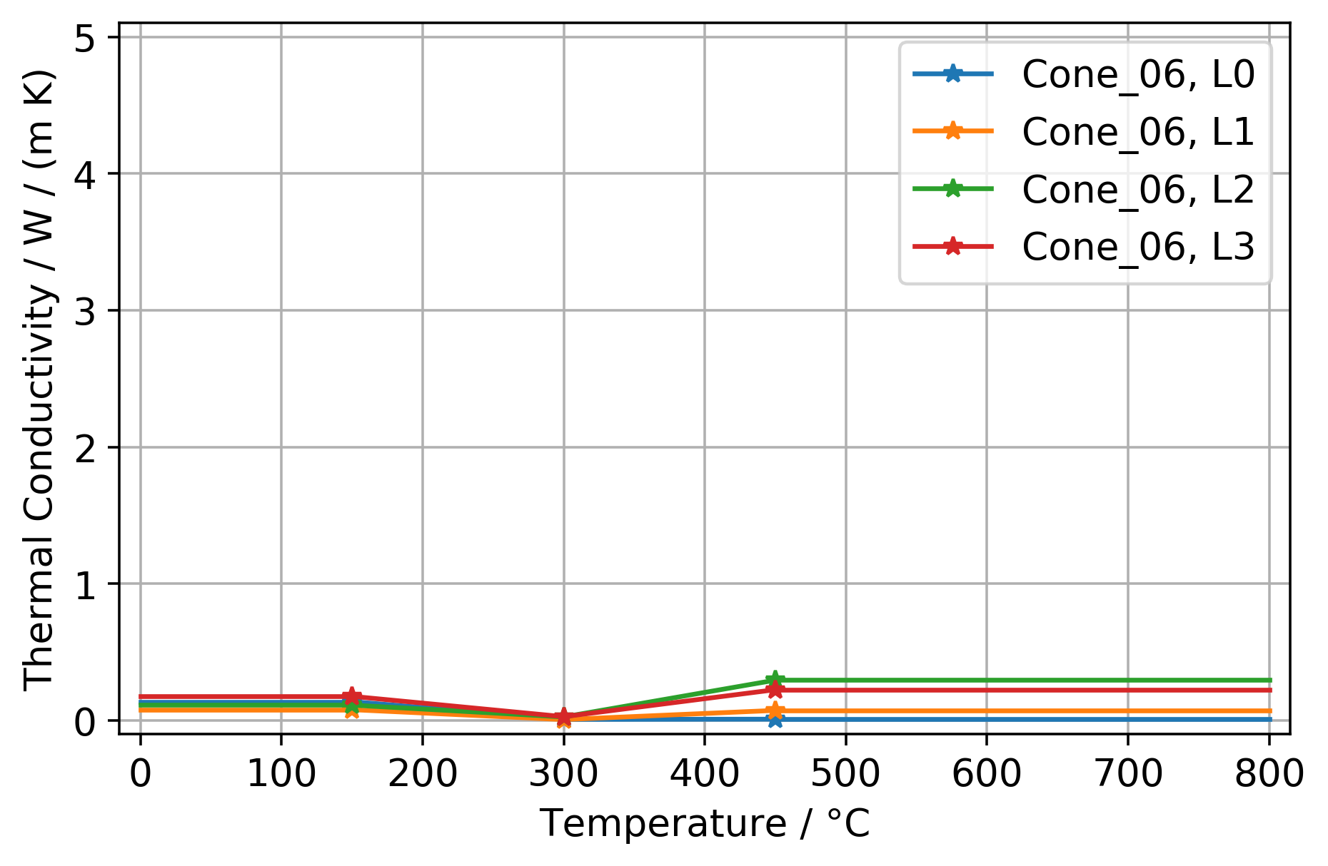
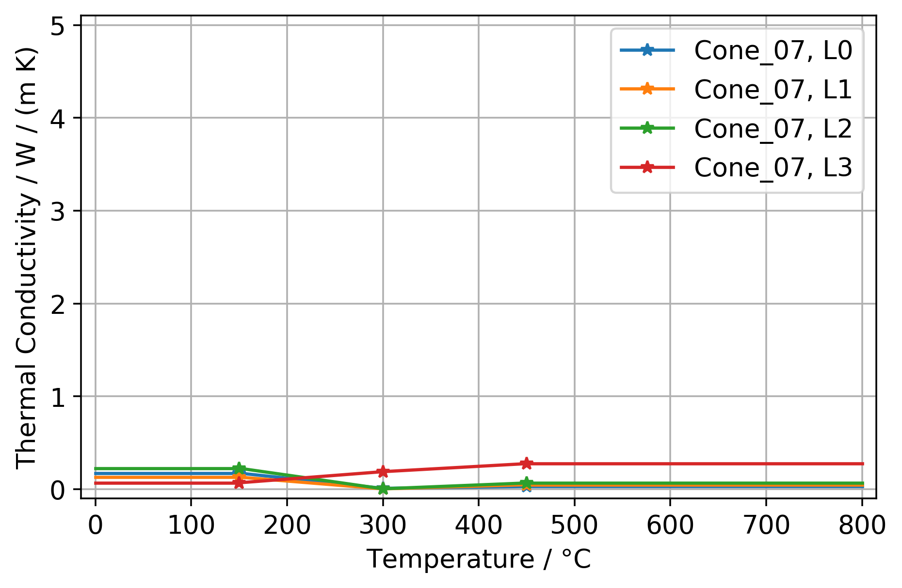
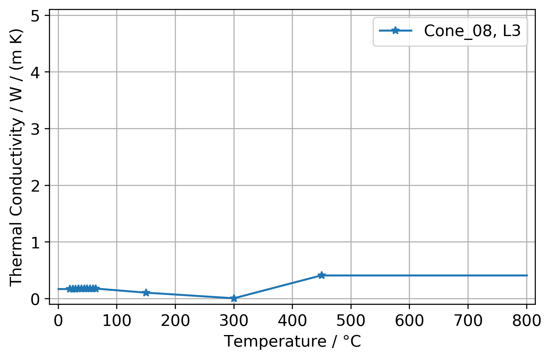
G.5 Specific Heat

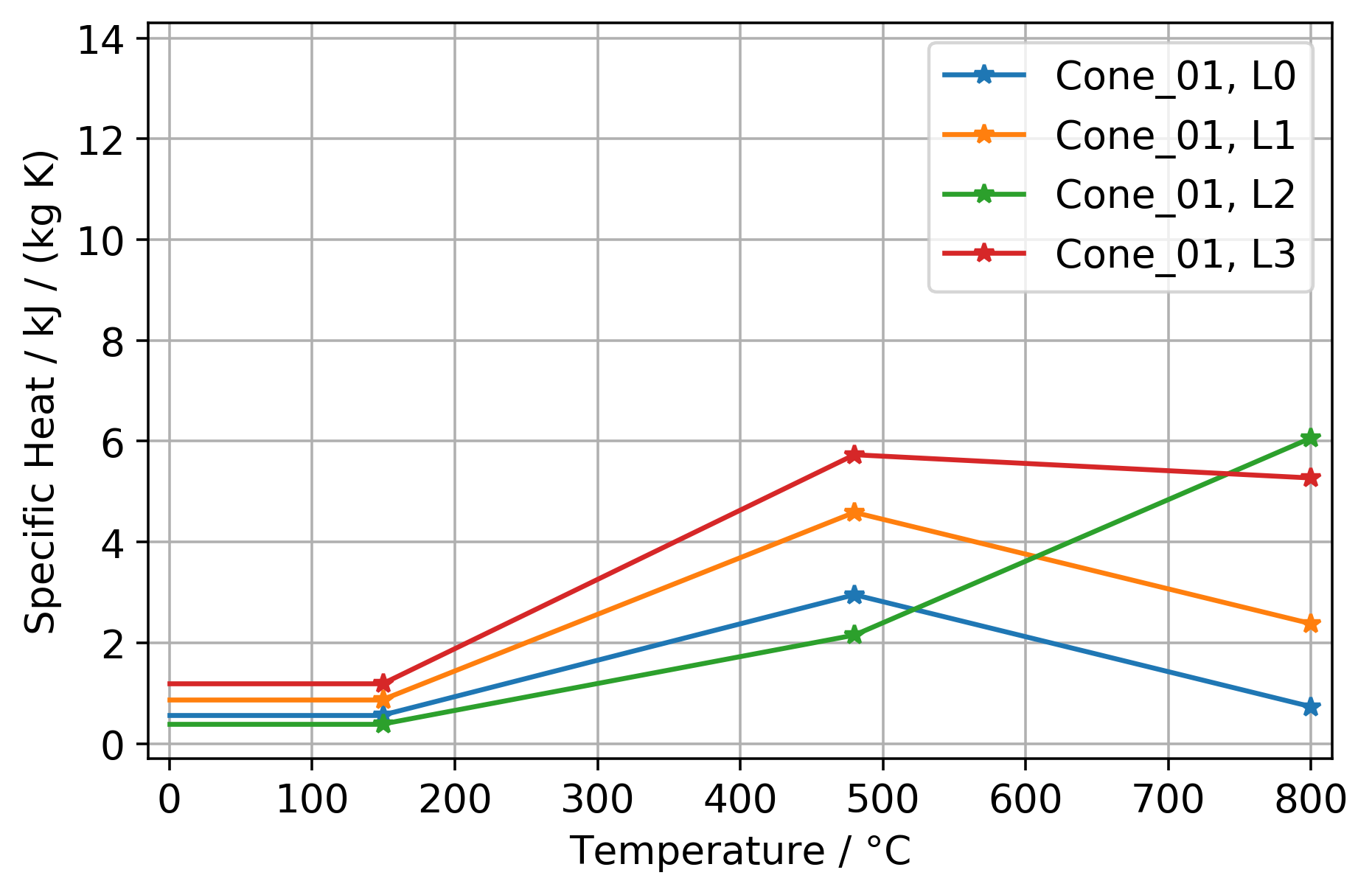
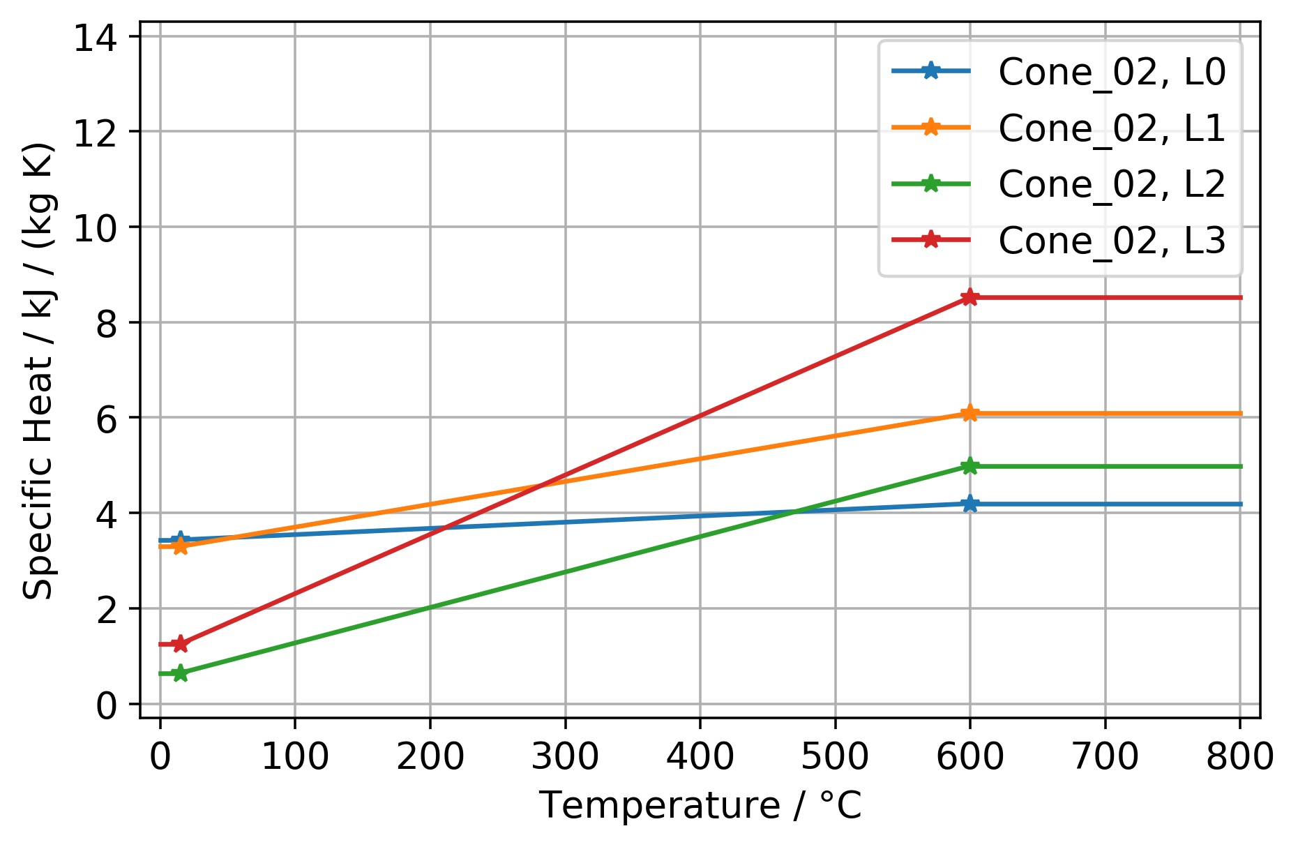
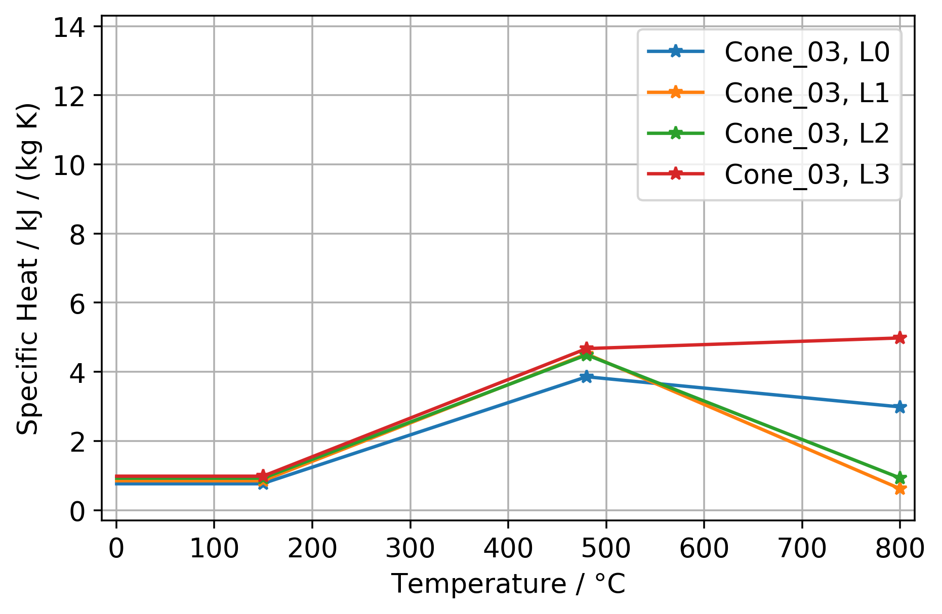
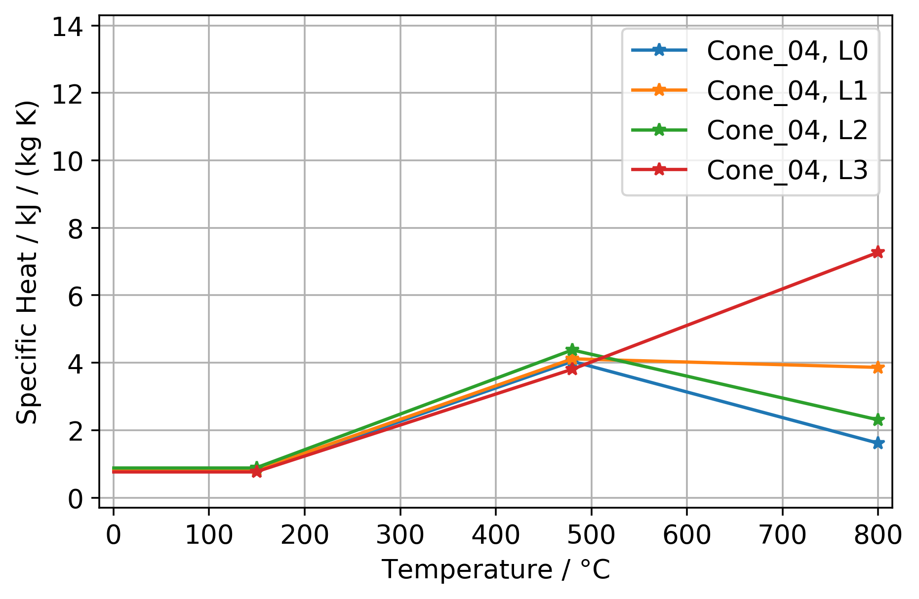
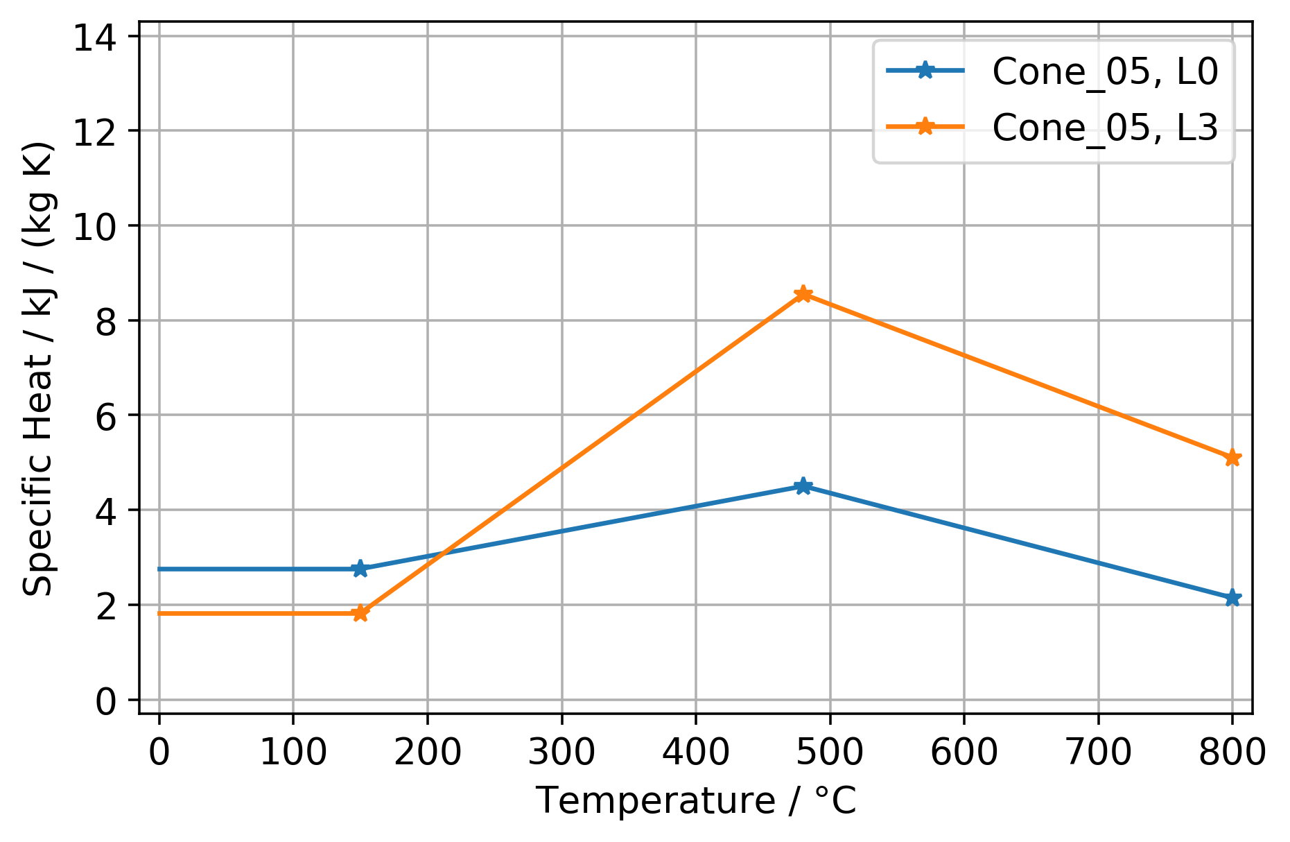
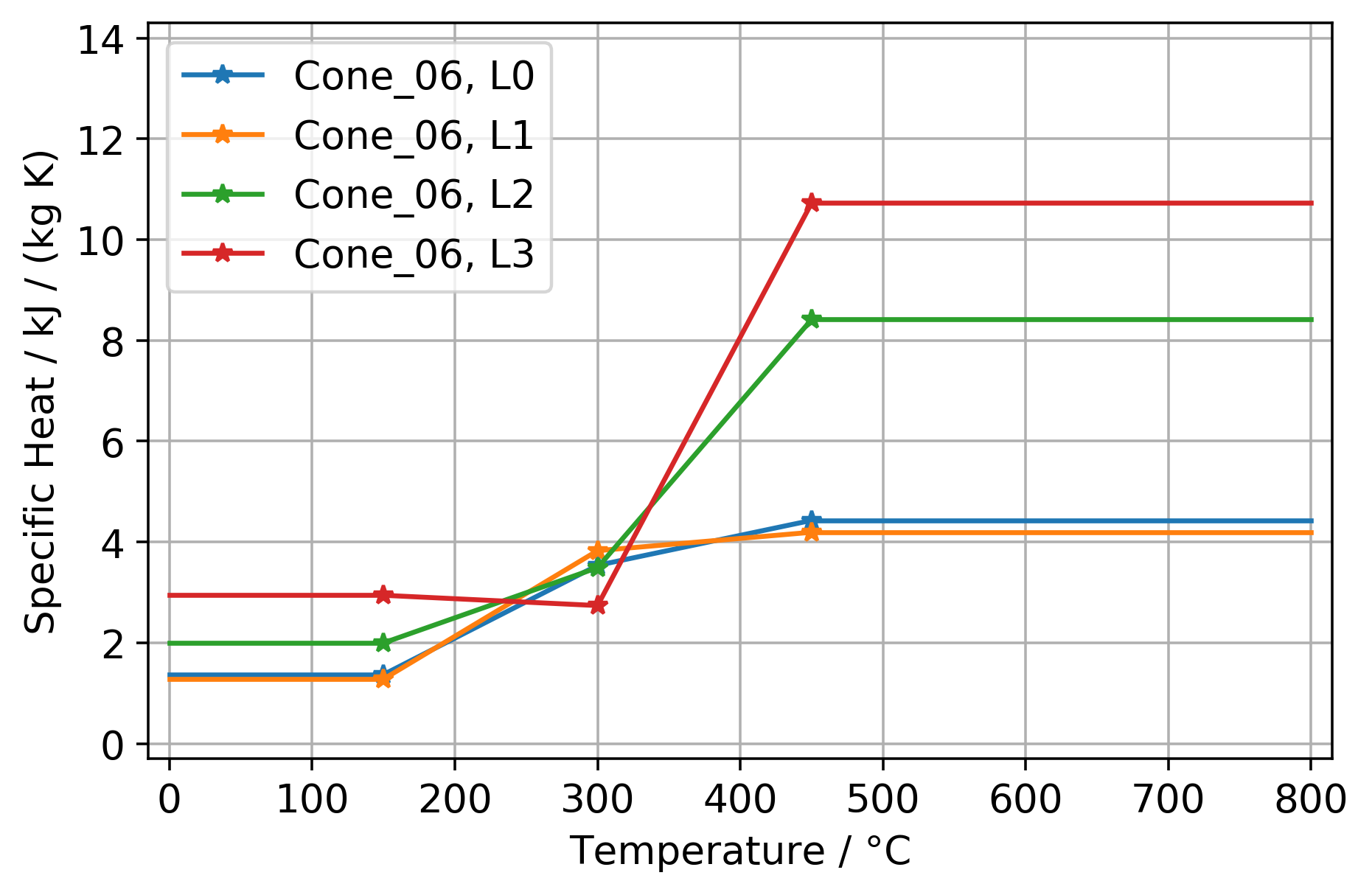
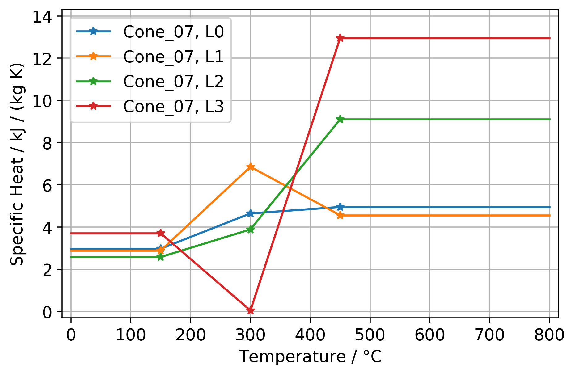
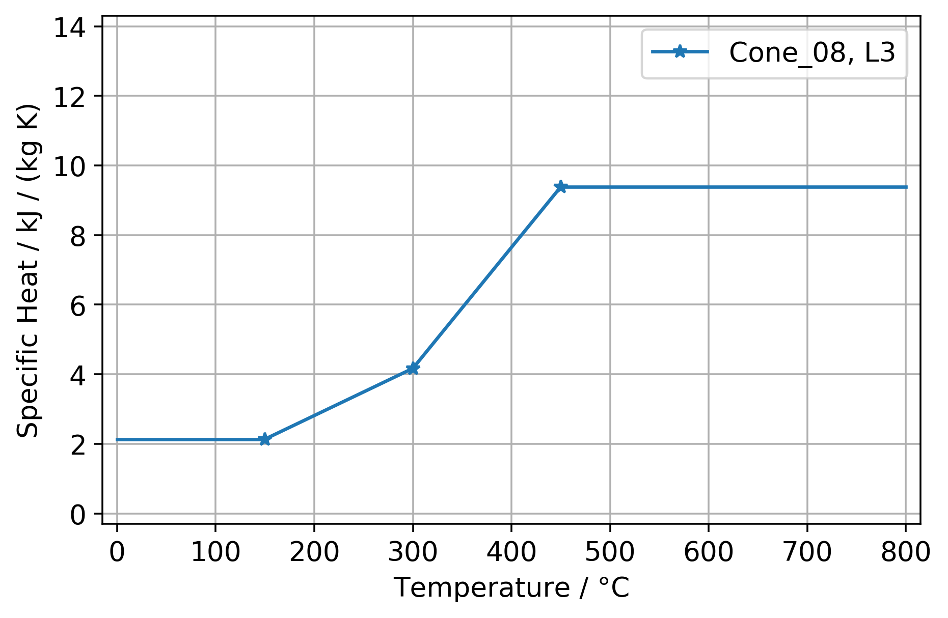
G.6 Residual Sample Mass

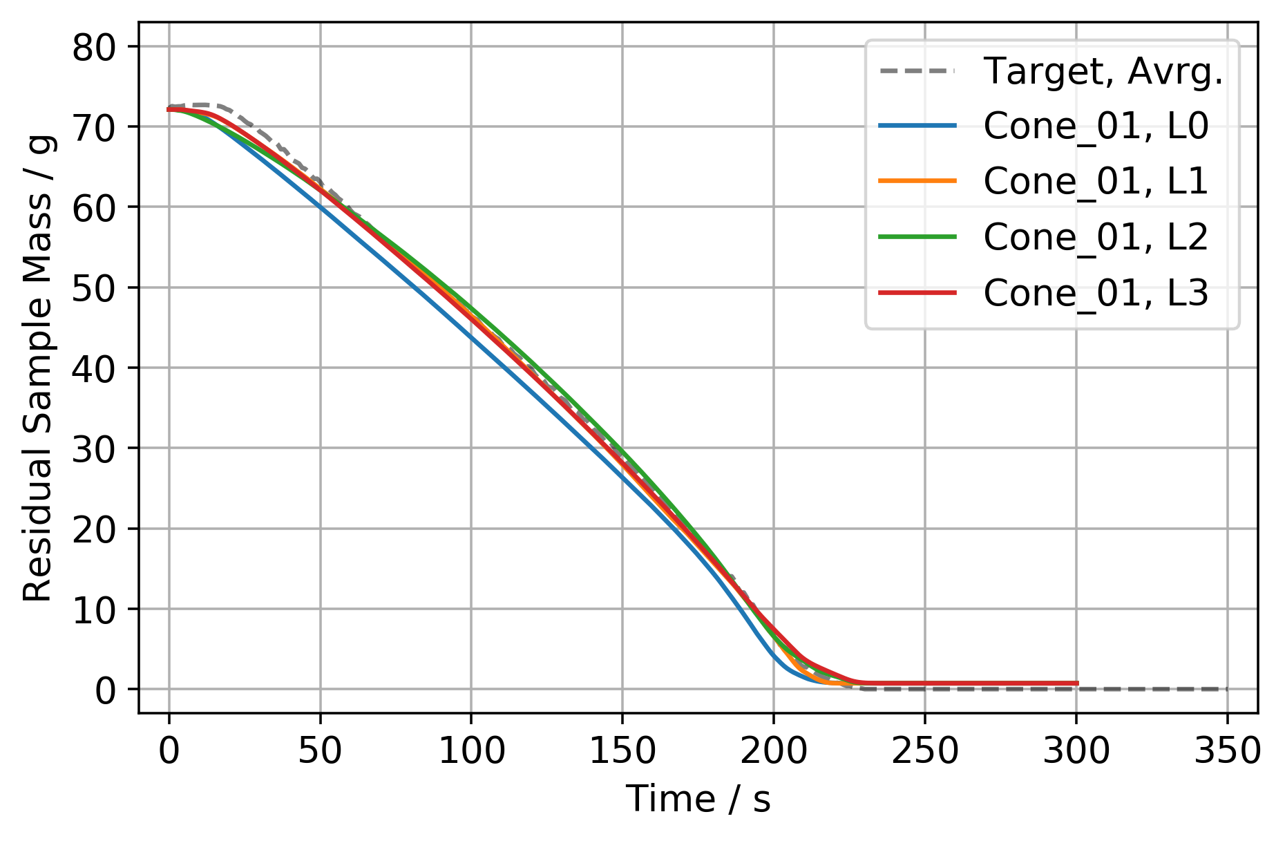
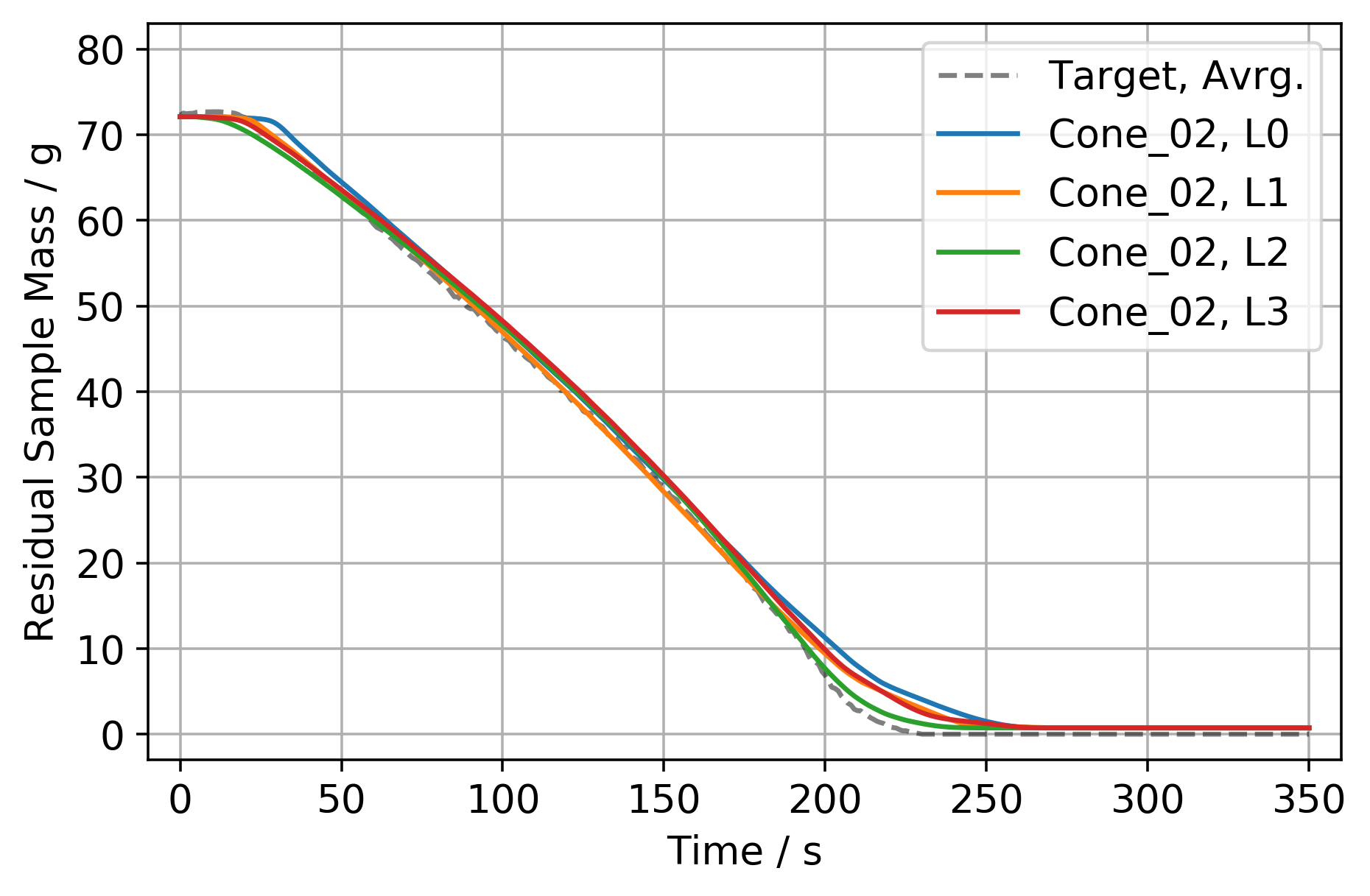
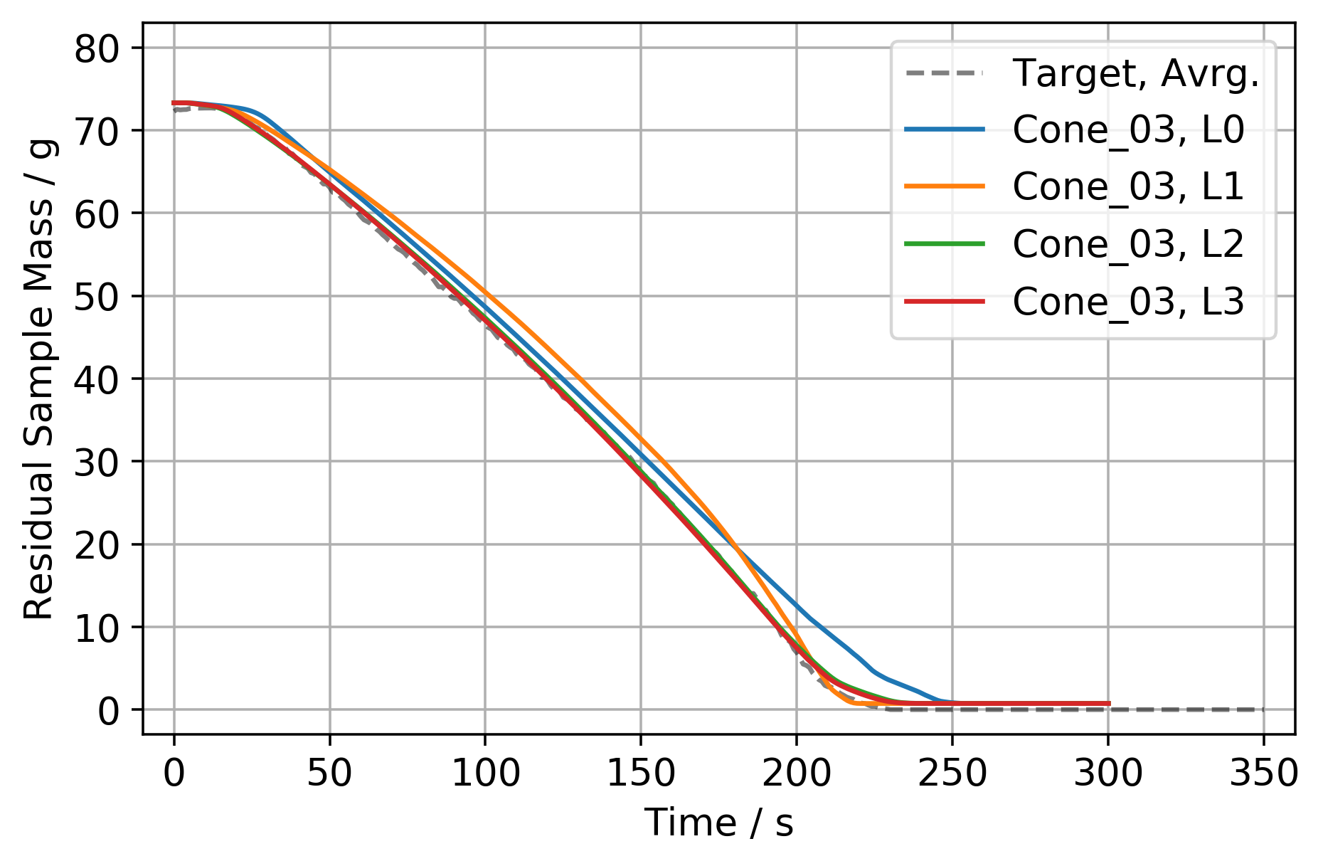
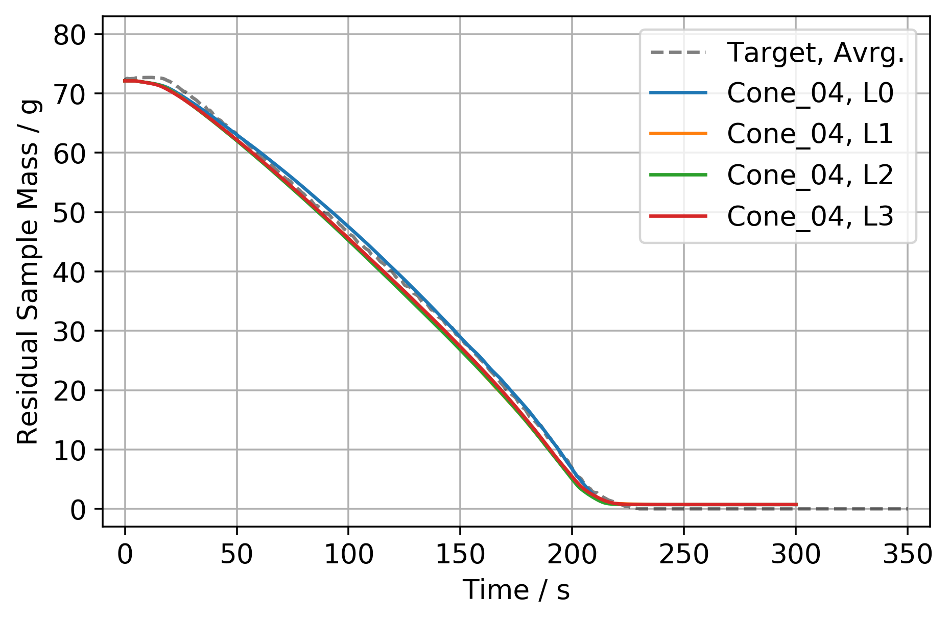
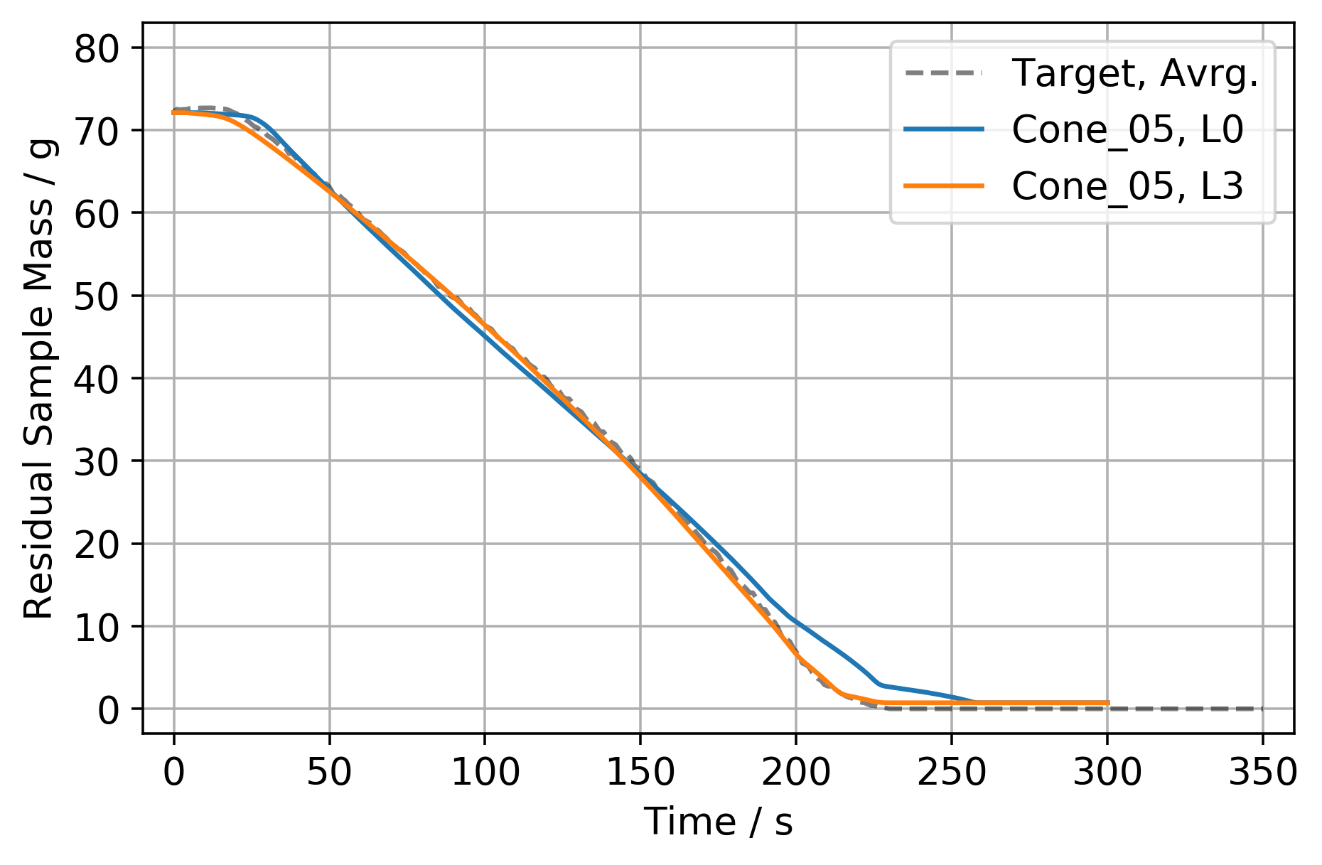
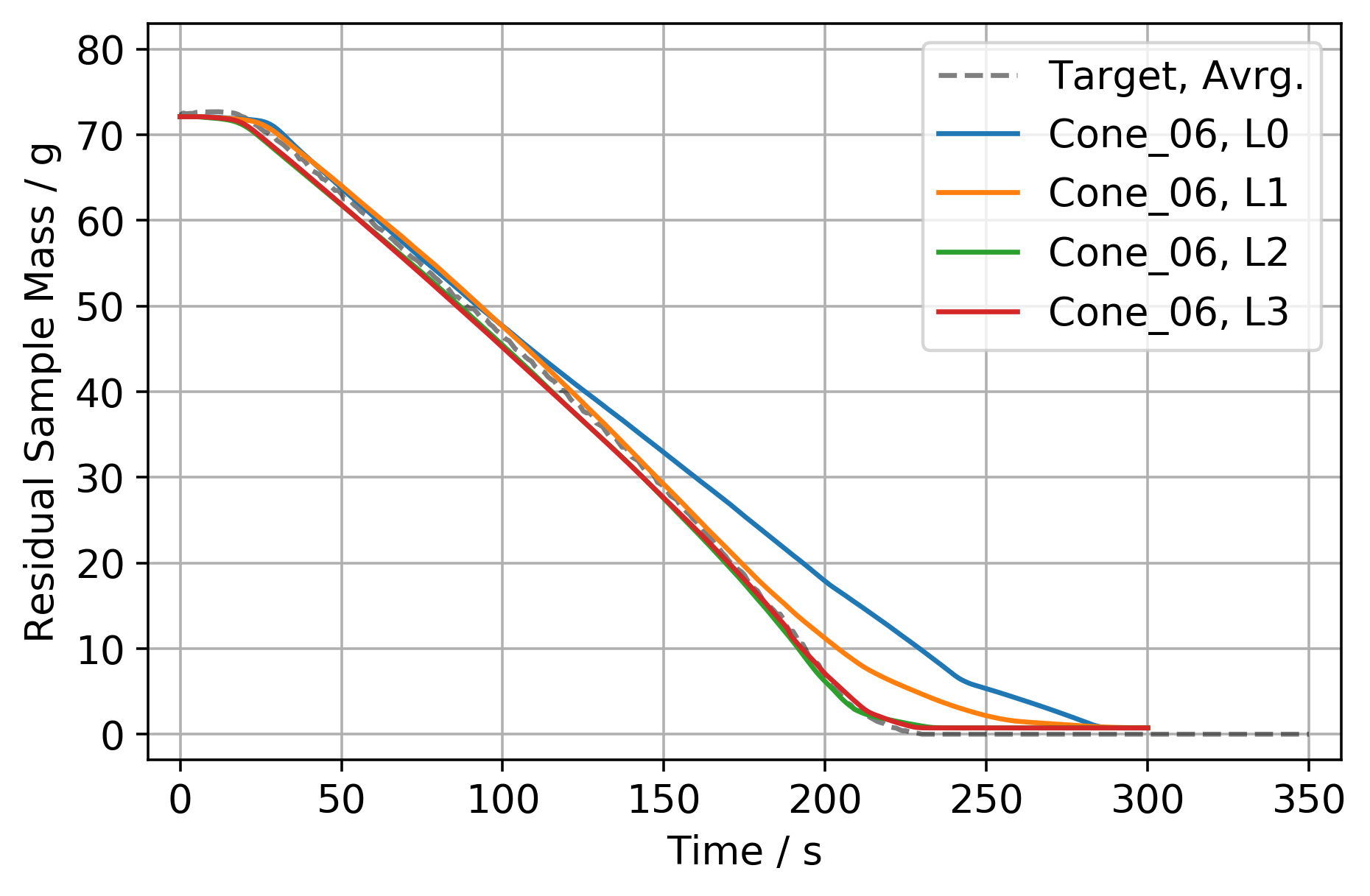
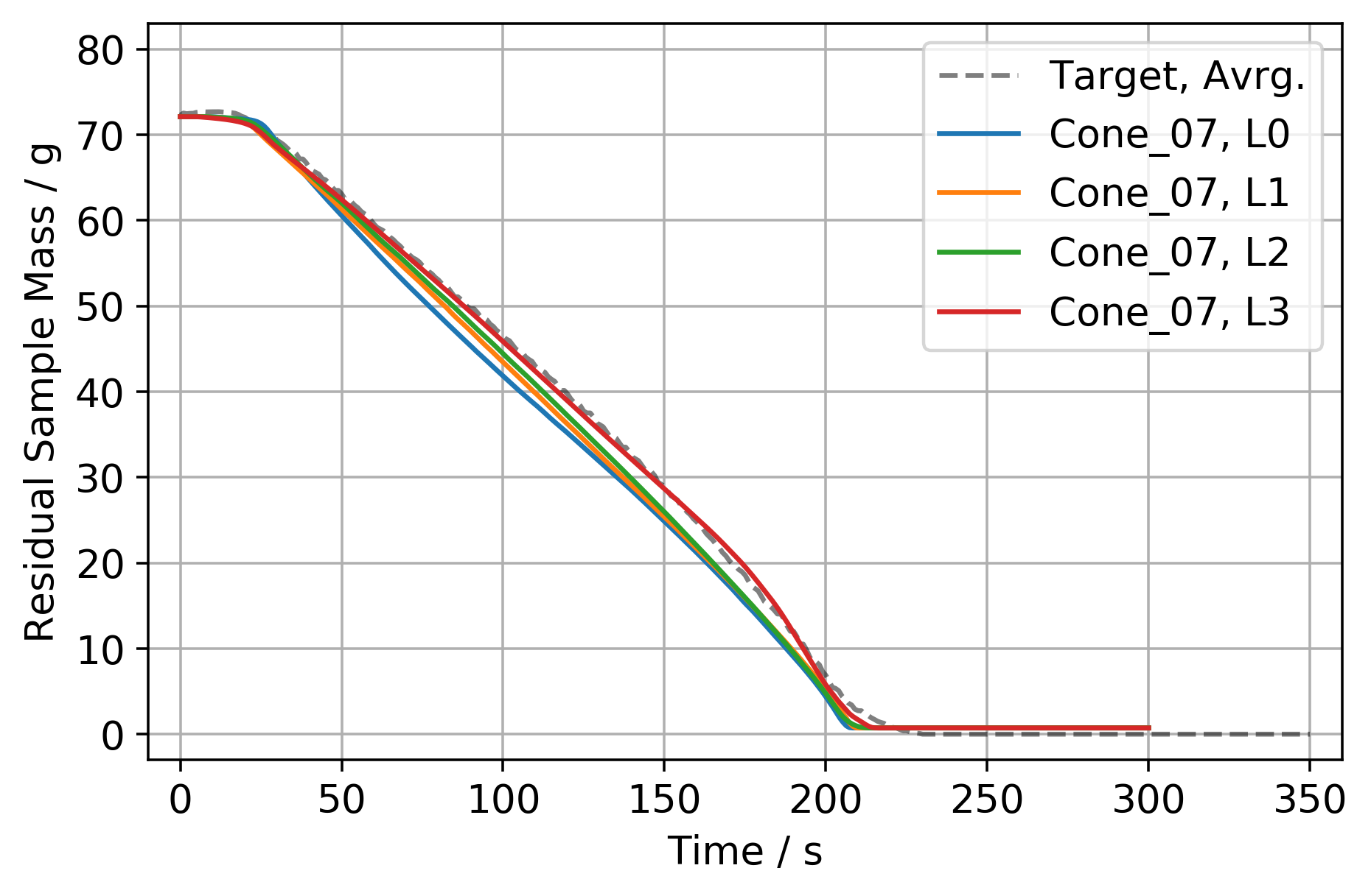
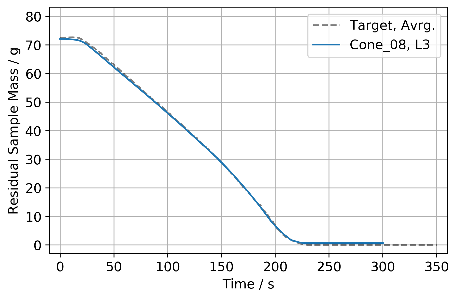
Appendix H Simple Cone Calorimeter Simulation – Fluid Cell Convergence

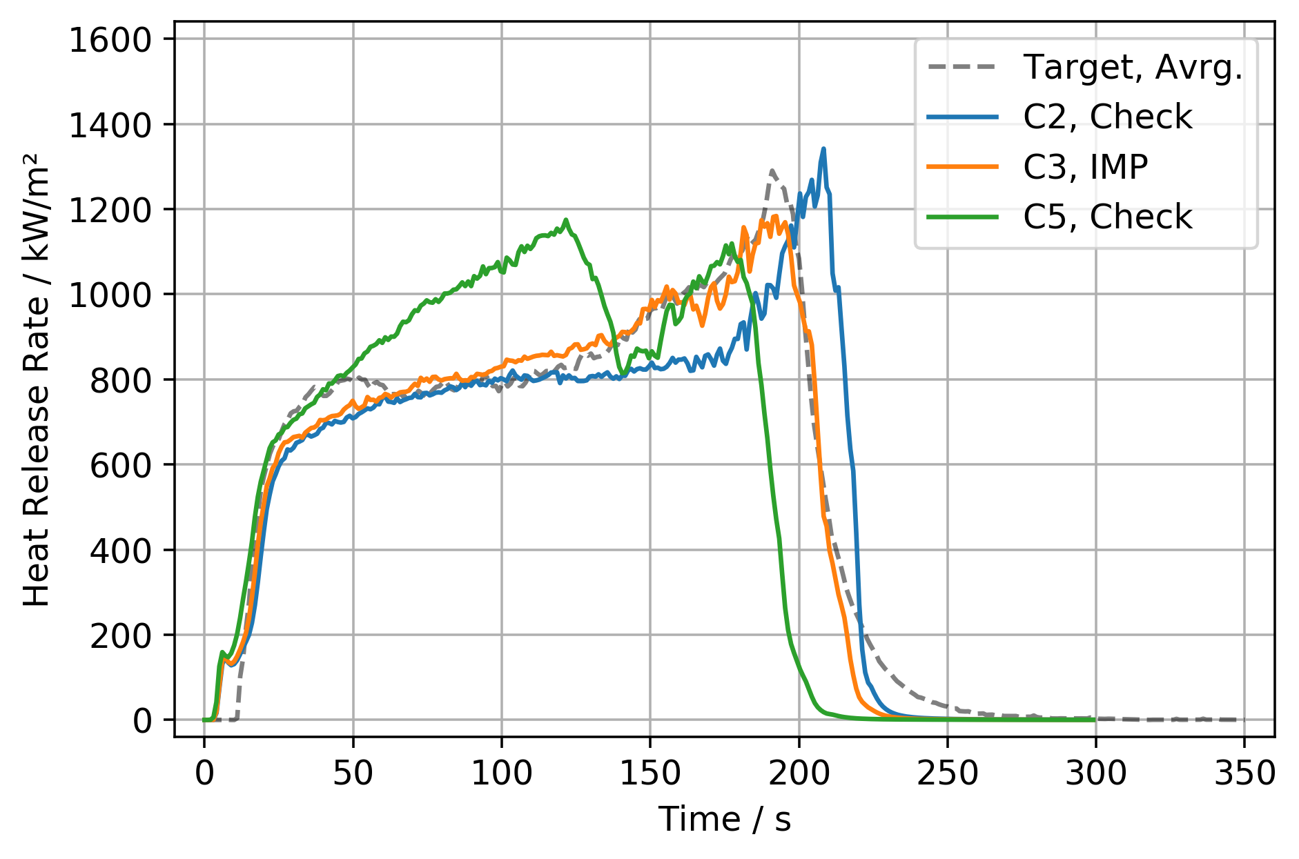
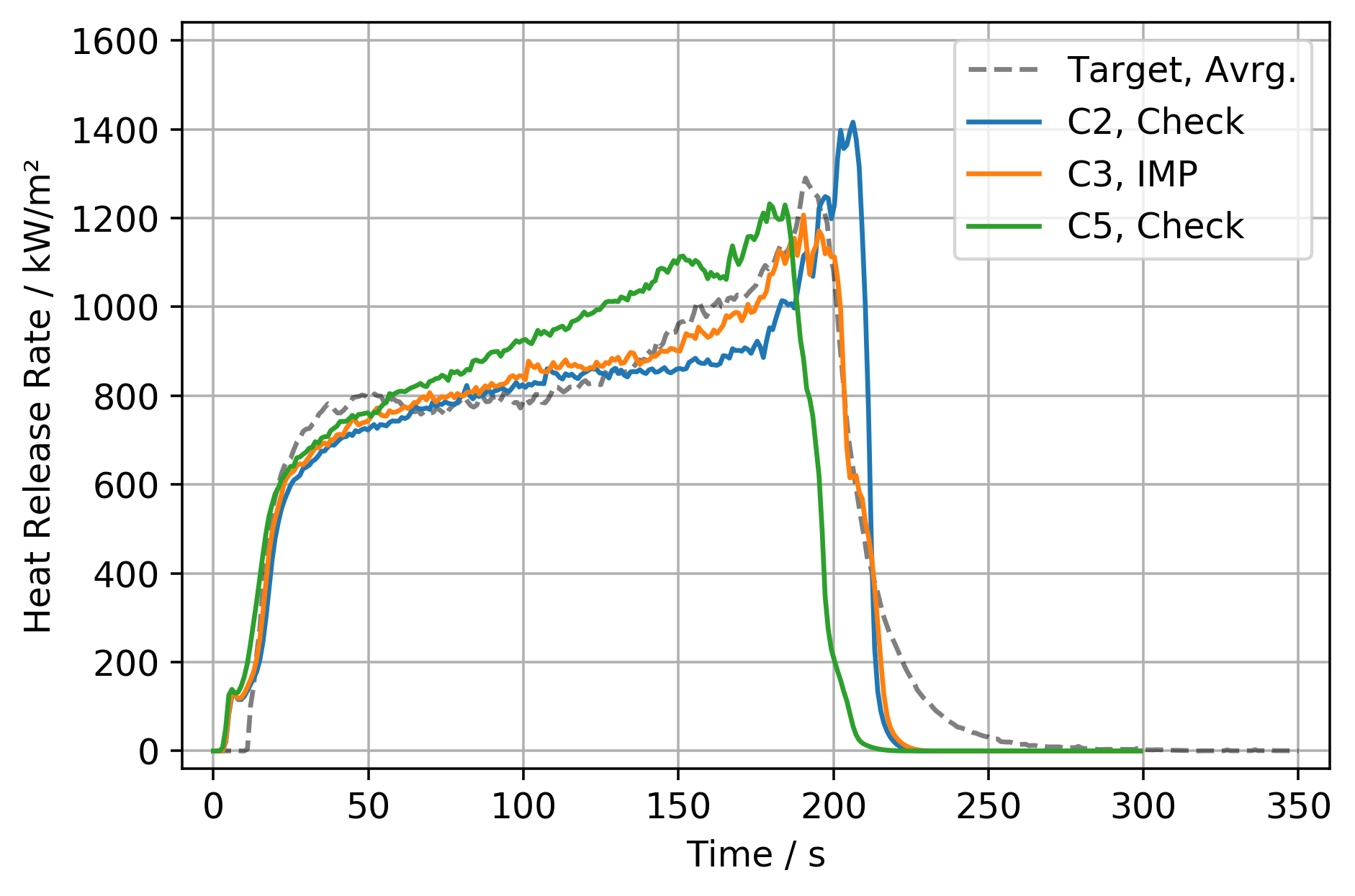
Appendix I Parallel Panel Simulation Results

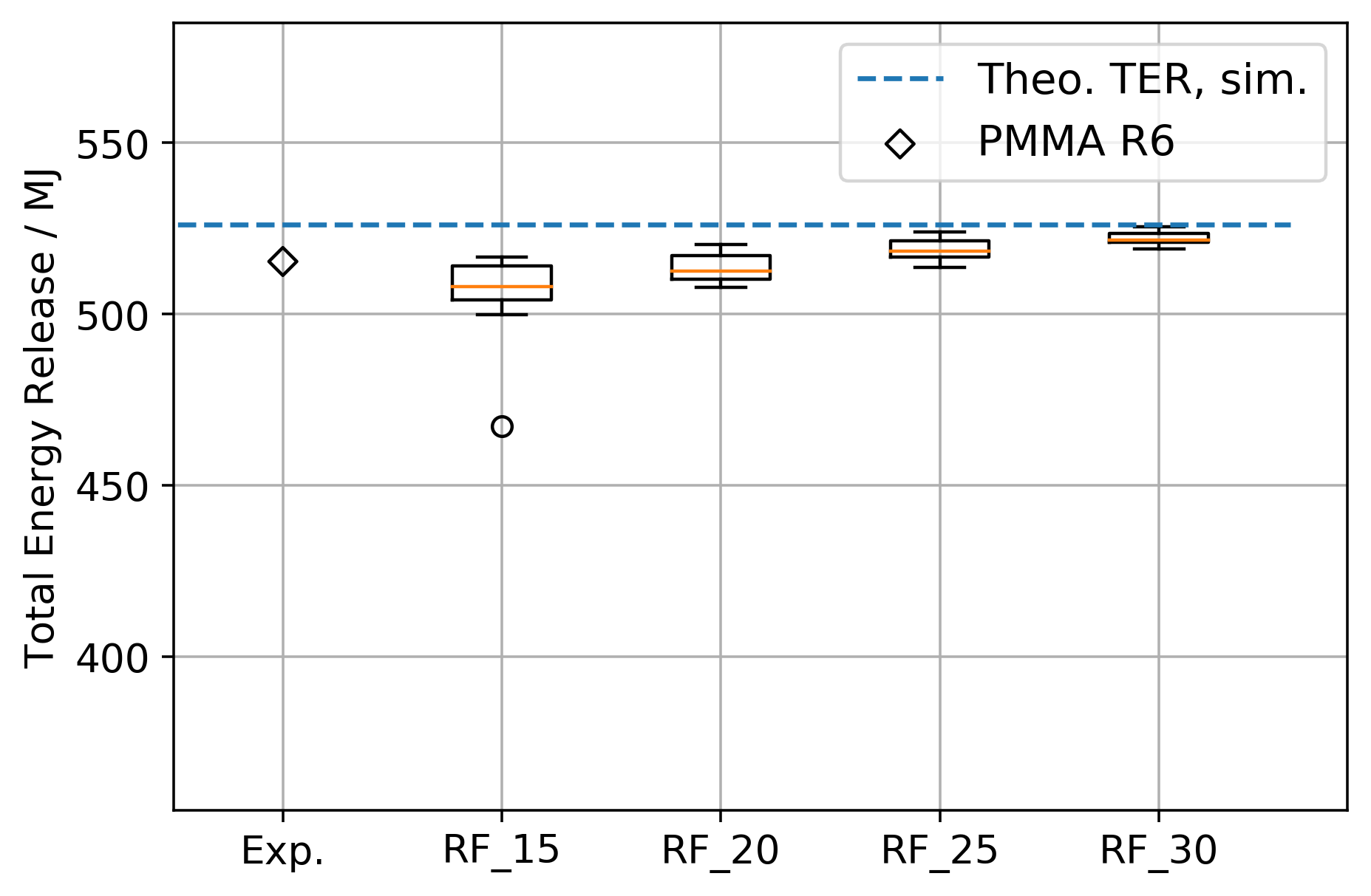
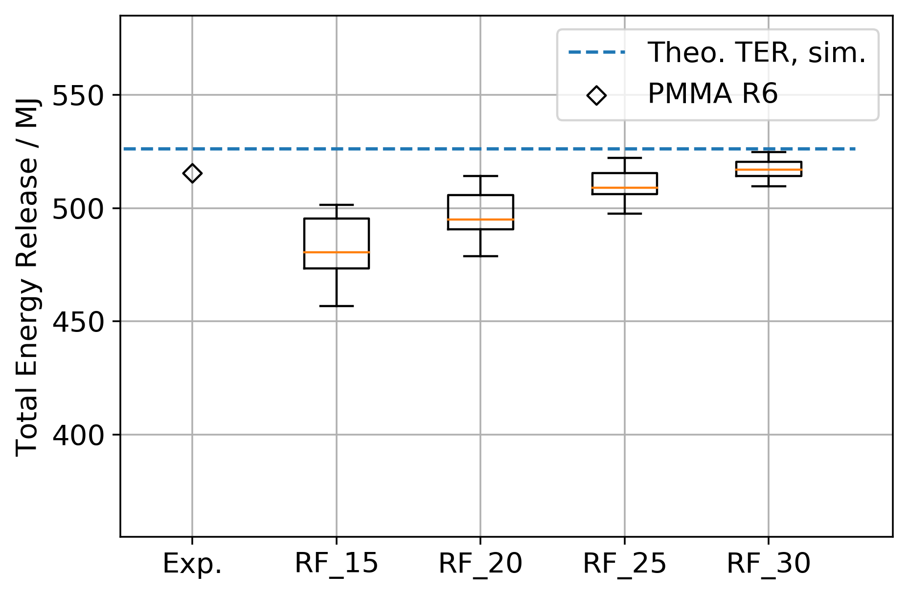
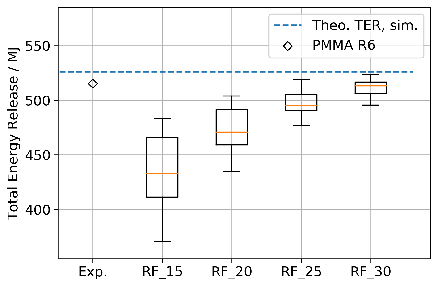
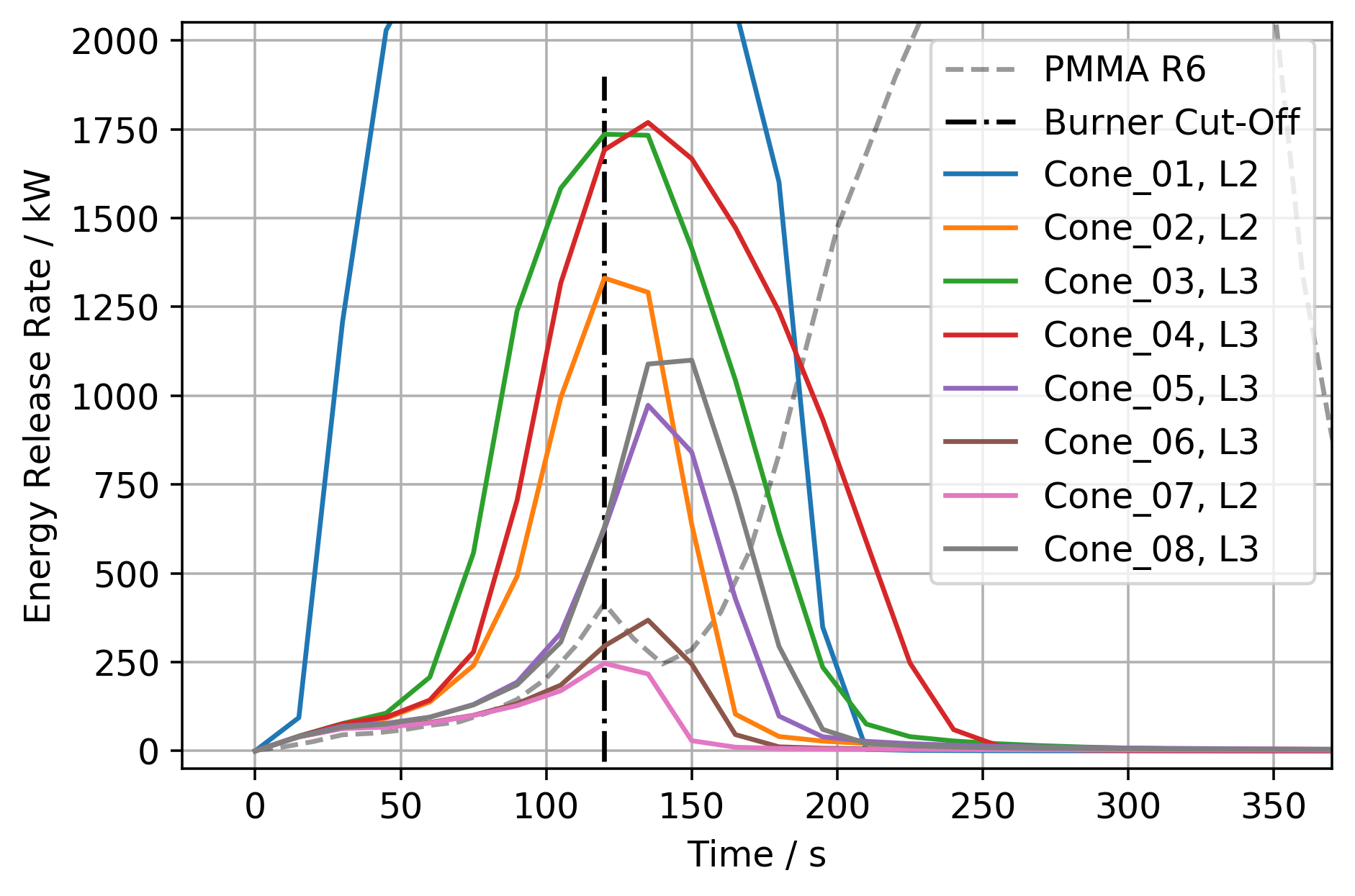
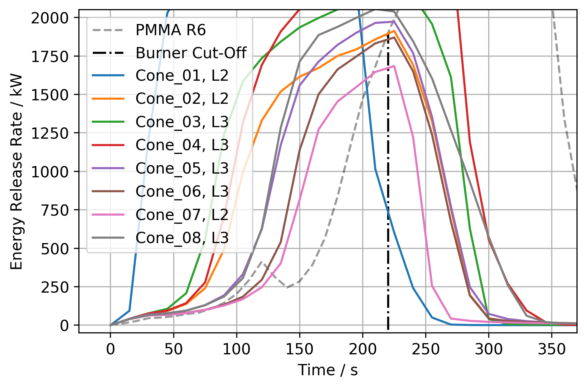
References

Matala [2013] Anna Matala. Methods and applications of pyrolysis modelling for polymeric materials. PhD thesis, Aalto University, Department of Mathematics and Systems Analysis Laboratory, Finland, 2013. URL http://urn.fi/URN:ISBN:978-951-38-8102-3.
Ding et al. [2019] Yan Ding, Stanislav I. Stoliarov, and Roland H. Kraemer. Pyrolysis model development for a polymeric material containing multiple flame retardants: Relationship between heat release rate and material composition. Combustion and Flame, 202:43–57, 04 2019. doi:10.1016/j.combustflame.2019.01.003.
Rogaume [2019] Thomas Rogaume. Thermal decomposition and pyrolysis of solid fuels: Objectives, challenges and modelling. Fire Safety Journal, 106:177 – 188, 05 2019. doi:10.1016/j.firesaf.2019.04.016.
Lautenberger et al. [2006] Chris Lautenberger, Guillermo Rein, and Carlos Fernandez-Pello. The application of a genetic algorithm to estimate material properties for fire modeling from bench-scale fire test data. Fire Safety Journal, 41(3):204 – 214, 2006. ISSN 0379-7112. doi:https://doi.org/10.1016/j.firesaf.2005.12.004. URL http://www.sciencedirect.com/science/article/pii/S0379711205001372.
Alonso et al. [2019] Alain Alonso, Mariano Lázaro, Pedro Lázaro, David Lázaro, and Daniel Alvear. Lldpe kinetic properties estimation combining thermogravimetry and differential scanning calorimetry as optimization targets. Journal of Thermal Analysis and Calorimetry, 138(4):2703–2713, Nov 2019. ISSN 1588-2926. doi:10.1007/s10973-019-08199-4. URL https://doi.org/10.1007/s10973-019-08199-4.
Lautenberger and Fernandez-Pello [2011] Chris Lautenberger and AC Fernandez-Pello. Optimization algorithms for material pyrolysis property estimation. Fire Safety Science, 10:751–764, 2011.
Batiot et al. [2022] B. Batiot, M. Bruns, S. Hostikka, I. Leventon, Y. Nakamura, P. Reszka, T. Rogaume, and S. Stoliarov. Measurement and Computation of Fire Phenomena (MaCFP) Condensed Phase Material Database. https://github.com/MaCFP/macfp-db, Commit: 7f89fd85f75cd2d4999c262f9b39f2f8109e12ef, DOI: https://doi.org/10.18434/mds2-2586, 2022.
Viitanen et al. [2022] Alexandra Viitanen, Simo Hostikka, and Jukka Vaari. CFD Simulations of Fire Propagation in Horizontal Cable Trays Using a Pyrolysis Model with Stochastically Determined Geometry. Fire Technology, July 2022. doi:10.1007/s10694-022-01291-6.
Rinta-Paavola and Hostikka [2022] Aleksi Rinta-Paavola and Simo Hostikka. A model for the pyrolysis of two nordic structural timbers. Fire and Materials, 46(1):55–68, 2022. doi:10.1002/fam.2947. URL https://onlinelibrary.wiley.com/doi/abs/10.1002/fam.2947.
Hehnen et al. [2020] Tristan Hehnen, Lukas Arnold, and Saverio La Mendola. Numerical Fire Spread Simulation Based on Material Pyrolysis – An Application to the CHRISTIFIRE Phase 1 Horizontal Cable Tray Tests. Fire, 3(3), 2020. ISSN 2571-6255. doi:10.3390/fire3030033. URL https://www.mdpi.com/2571-6255/3/3/33.
Hostikka and Matala [2017] Simo Hostikka and Anna Matala. Pyrolysis model for predicting the heat release rate of birch wood. Combustion Science and Technology, 189(8):1373–1393, 8 2017. ISSN 0010-2202. doi:10.1080/00102202.2017.1295959.
Alonso et al. [2023] Alain Alonso, David Lázaro, Mariano Lázaro, and Daniel Alvear. Numerical prediction of cables fire behaviour using non-metallic components in cone calorimeter. Combustion Science and Technology, 0(0):1–17, 2023. doi:10.1080/00102202.2023.2182198. URL https://doi.org/10.1080/00102202.2023.2182198.
Korobeinichev et al. [2019] O.P. Korobeinichev, A.A. Paletsky, M.B. Gonchikzhapov, R.K. Glaznev, I.E. Gerasimov, Y.K. Naganovsky, I.K. Shundrina, A.Yu. Snegirev, and R. Vinu. Kinetics of thermal decomposition of PMMA at different heating rates and in a wide temperature range. Thermochimica Acta, 671:17–25, 2019. ISSN 0040-6031. doi:10.1016/j.tca.2018.10.019. URL https://www.sciencedirect.com/science/article/pii/S0040603118303460.
Zeng et al. [2002] W. R. Zeng, S. F. Li, and W. K. Chow. Review on chemical reactions of burning poly(methyl methacrylate) pmma. Journal of Fire Sciences, 20(5):401–433, September 2002. doi:10.1177/0734904102020005482.
Fiola et al. [2021] Gregory J. Fiola, Dushyant M. Chaudhari, and Stanislav I. Stoliarov. Comparison of Pyrolysis Properties of Extruded and Cast Poly(methyl methacrylate). Fire Safety Journal, 120, 2021. ISSN 0379-7112. doi:https://doi.org/10.1016/j.firesaf.2020.103083. URL https://www.sciencedirect.com/science/article/pii/S0379711219307301. Fire Safety Science: Proceedings of the 13th International Symposium.
Karpov et al. [2018] Alexander I. Karpov, Oleg P. Korobeinichev, Artem A. Shaklein, Andrey A. Bolkisev, Amit Kumar, and Andrey G. Shmakov. Numerical study of horizontal flame spread over PMMA surface in still air. Applied Thermal Engineering, 144:937–944, 2018. ISSN 1359-4311. doi:https://doi.org/10.1016/j.applthermaleng.2018.08.106. URL https://www.sciencedirect.com/science/article/pii/S1359431118335750.
Karpov et al. [2015] Alexander Karpov, Artem Shaklein, Mikhail Korepanov, and Artem Galat. Numerical Study of the Radiative and Turbulent Heat Flux Behavior of Upward Flame Spread Over PMMA. In Kazunori Harada, Ken Matsuyama, Keisuke Himoto, Yuji Nakamura, and Kaoru Wakatsuki, editors, Fire Science and Technology 2015, pages 841–848, Singapore, 2015. Springer Singapore. ISBN 978-981-10-0376-9.
Wu et al. [2003] K.K. Wu, W.F. Fan, C.H. Chen, T.M. Liou, and I.J. Pan. Downward flame spread over a thick PMMA slab in an opposed flow environment: experiment and modeling. Combustion and Flame, 132(4):697–707, 2003. ISSN 0010-2180. doi:https://doi.org/10.1016/S0010-2180(02)00520-5. URL https://www.sciencedirect.com/science/article/pii/S0010218002005205.
Rauwoens et al. [2010] P. Rauwoens, J. Degroote, S. Wasan, J. Vierendeels, and B Merci. Upward Flame Spread Simulations by Coupling an Enthalpy-Based Pyrolysis Model with CFD. In Proceedings of the 6th International Seminar on Fire and Explosion Hazards, pages 241–251, Leeds, UK, 2010.
Kwon [2006] Jae-Wook Kwon. Evaluation of FDS V.4: Upward Flame Spread. Master’s thesis, Worcester Polytechnic Institute, Fire Protection Engineering, MA, USA, 2006. URL https://web.wpi.edu/Pubs/ETD/Available/etd-090606-112948/.
Chaudhari et al. [2021] Dushyant M. Chaudhari, Gregory J. Fiola, and Stanislav I. Stoliarov. Experimental analysis and modeling of buoyancy-driven flame spread on cast poly(methyl methacrylate) in corner configuration. Polymer Degradation and Stability, 183:109433, 2021. ISSN 0141-3910. doi:https://doi.org/10.1016/j.polymdegradstab.2020.109433. URL https://www.sciencedirect.com/science/article/pii/S0141391020303621.
Stoliarov and Lyon [2008] Stanislav I. Stoliarov and Richard E. Lyon. Thermo-kinetic model of burning for pyrolyzing materials. In Fire Safety Science – Proceedings of the Ninth Internatinoal Symposium, Karlsruhe, Germany, page 1141–1152, 2008. doi:10.3801/iafss.fss.9-1141.
McGrattan et al. [2021a] Kevin McGrattan, Simo Hostikka, Jason Floyd, Randall McDermott, and Marcos Vanella. Fire Dynamics Simulator User’s Guide, 05 2021a.
Moinuddin et al. [2020] Khalid Moinuddin, Qazi Samia Razzaque, and Ananya Thomas. Numerical simulation of coupled pyrolysis and combustion reactions with directly measured fire properties. Polymers, 12(9), 2020. ISSN 2073-4360. doi:10.3390/polym12092075. URL https://www.mdpi.com/2073-4360/12/9/2075.
Boulet et al. [2012] P. Boulet, G. Parent, Z. Acem, T. Rogaume, T. Fateh, J. Zaida, and F. Richard. Characterization of the radiative exchanges when using a cone calorimeter for the study of the plywood pyrolysis. Fire Safety Journal, 51:53–60, 2012. ISSN 0379-7112. doi:10.1016/j.firesaf.2012.03.003. URL https://www.sciencedirect.com/science/article/pii/S037971121200046X.
Hostikka and Axelsson [2003] Simo Hostikka and Jesper Axelsson. Modelling of the radiative feedback from the flames in cone calorimeter. Technical report, NORDTEST, 2003. URL https://www.nordtest.info/wp/2003/10/02/modelling-of-the-radiative-feedback-from-the-flames-in-cone-calorimeter-nt-tr-540/.
Leventon et al. [2022] I.T. Leventon, M.V. Heck, K.B. McGrattan, M.F. Bundy, and R.D. Davis. Experimental Measurements for Fire Model Validation - Parallel Panel Tests on PMMA. https://github.com/MaCFP/macfp-db/tree/master/Fire_Growth/NIST_Parallel_Panel, Commit: 25614bd527b658fca72265ed2940ea1287e83343, DOI: https://doi.org/10.18434/mds2-2812, 2022.
Hehnen and Arnold [2023] Tristan Hehnen and Lukas Arnold. PMMA Pyrolysis Simulation – from Micro- to Real-Scale – Dataset. Technical report, Forschungszentrum Jülich and Bergische Universität Wuppertal, Germany, January 2023. URL https://zenodo.org/record/7065338.
Hehnen [2022] Tristan Hehnen. PMMA Pyrolysis and Fire Propagation in FDS. www.youtube.com/@firesimandcoding;
www.youtube.com/playlist?list=PLWziITJoPnJKtVuaVudyO2Lz-OWaCE9Co, 2022.
McGrattan et al. [2021b] Kevin McGrattan, Simo Hostikka, Jason Floyd, Randall McDermott, and Marcos Vanella. Fire Dynamics Simulator Technical Reference Guide Volume 1: Mathematical Model, 05 2021b.
Duan et al. [1993] Qingyun Duan, Vijai K. Gupta, and Soroosh Sorooshian. Shuffled complex evolution approach for effective and efficient global minimization. Journal of optimization theory and applications, 76(3):501–521, 1993.
Arnold et al. [2018a] Lukas Arnold, Tristan Hehnen, Patrick Lauer, Corinna Trettin, and Ashish Vinayak. PROPTI – A Generalised Inverse Modelling Framework. In Journal of Physics: Conference Series, volume 1107, page 032016. IOP Publishing, 2018a.
Arnold et al. [2019] Lukas Arnold, Tristan Hehnen, Patrick Lauer, Corinna Trettin, and Ashish Vinayak. Application cases of inverse modelling with the PROPTI framework. Fire Safety Journal, page 102835, 2019. ISSN 0379-7112. doi:10.1016/j.firesaf.2019.102835. URL http://www.sciencedirect.com/science/article/pii/S0379711219300438.
Arnold et al. [2018b] Lukas Arnold, Tristan Hehnen, Patrick Lauer, Corinna Trettin, and Ashish Vinayak. PROPTI. Technical report, Forschungszentrum Jülich and Bergische Universität Wuppertal, Germany, March 2018b. URL https://zenodo.org/record/1438349.
Houska et al. [2015] Tobias Houska, Philipp Kraft, Alejandro Chamorro-Chavez, and Lutz Breuer. Spotting model parameters using a ready-made python package. PLoS ONE, 10:e0145180, 12 2015. URL doi:10.1371/journal.pone.0145180.
McNeill [1994] Ian C. McNeill. Products of Thermal Degradation in Polymer Systems Based on Methyl Methacrylate. International Journal of Polymeric Materials and Polymeric Biomaterials, 24(1-4):31–45, 1994. doi:10.1080/00914039408028548.
Bowman [2019] Graig T. Bowman. Non-equilibirum radical concentrations in shock-initiated methane oxidation. Fire Safety Journal, page 102835, 2019. ISSN 0379-7112. doi:10.1016/j.firesaf.2019.102835. URL http://www.sciencedirect.com/science/article/pii/S0379711219300438.
Zhukov and Kong [2018] Victor P. Zhukov and Alan F. Kong. A compact reaction mechanism of methane oxidation at high pressures. Progress in Reaction Kinetics and Mechanism, 43(1):62–78, 2018. doi:10.3184/146867818X15066862094914. URL https://doi.org/10.3184/146867818X15066862094914.
Zhukov et al. [2005] Victor P. Zhukov, V. A. Sechenov, and A. Yu. Starikovskii. Autoignition of a lean propane-air mixture at high pressures. Kinetics and Catalysis, 46(3):319–327, 2005. doi:10.1007/s10975-005-0079-7. URL https://doi.org/10.1007/s10975-005-0079-7.
Westbrook et al. [2002] C.K. Westbrook, W.J. Pitz, J.E. Boercker, H.J. Curran, J.F. Griffiths, C. Mohamed, and M. Ribaucour. Detailed chemical kinetic reaction mechanisms for autoignition of isomers of heptane under rapid compression. Proceedings of the Combustion Institute, 29(1):1311–1318, 2002. ISSN 1540-7489. doi:10.1016/S1540-7489(02)80161-4. URL https://www.sciencedirect.com/science/article/pii/S1540748902801614. Proceedings of the Combustion Institute.
Wolfhard and Parker [1949] H. G. Wolfhard and W. G. Parker. A new technique for the spectroscopic examination of flames at normal pressures. Proceedings of the Physical Society. Section A, 62(11):722–730, nov 1949. doi:10.1088/0370-1298/62/11/305.
Curran [2019] Henry J. Curran. Developing detailed chemical kinetic mechanisms for fuel combustion. Proceedings of the Combustion Institute, 37(1):57–81, 2019. ISSN 1540-7489. doi:10.1016/j.proci.2018.06.054. URL https://www.sciencedirect.com/science/article/pii/S1540748918302372.
Lannoye et al. [2023] Karen De Lannoye, Corinna Trettin, Alexander Belt, E.A. Reinecke, Roland Goertz, and Lukas Arnold. The Influence of Experimental Conditions on the Mass Loss for TGA in Fire Safety Science. Submitted to: Fire Safety Journal, 2023.
McGrattan et al. [2021c] Kevin McGrattan, Simo Hostikka, Jason Floyd, Randall McDermott, and Marcos Vanella. Fire Dynamics Simulator Technical Reference Guide Volume 3: Validation, 05 2021c.
Quintiere [2017] James G. Quintiere. Principles of Fire Behavior, Second Edition. CRC Press, 2017. ISBN 9781498735629.
Babrauskas [1982] Vyto Babrauskas. Development of the Cone Calorimeter: A Bench-Scale Heat Release Rate Apparatus Based on Oxygen Consumption. Technical report, National Institute of Standards and Technology, Gaithersburg, MD, 1982-11-01 1982.
iso [2015] ISO 5660-1:2015(E) — Part 1: Heat release rate (cone calorimeter method) and smoke production rate. ISO, 2015.
Brännström [2016] Fabian Brännström. Application of fire simulation within the railway industry. In 14th International Conference and Exhibition on Fire Science and Engineering. Interflam, July 2016.
De Lannoye et al. [2023] Karen De Lannoye, Alexander Belt, Ernst-Arndt Reinecke, Frank Markert, and Lukas Arnold. Comparison of Black and Transparent PMMA in the Cone Calorimeter. In Morgan C. Bruns and Marc L. Janssens, editors, ASTM SELECTED TECHNICAL PAPERS STP1642: Obtaining Data for Fire Growth Models, page 150–160. ASTM International, March 2023. doi:10.1520/STP164220210105.
Elliott et al. [2014] Angus Elliott, Alastair Temple, Cristian Maluk, and Luke Bisby. Novel Testing to Study the Performance of Intumescent Coatings under Non-Standard Heating Regimes. In Fire Safety Science, volume 11, pages 652–665, 02 2014. doi:10.3801/IAFSS.FSS.11-652.
Quaresma [2023] Tássia Quaresma. Sensitivity analysis of simulation input parameters, a comparison between flame spread and cone calorimeter setups. In European Conference & Expo on Fire Safety Engineering, SFPE23. SFPE, March 2023.
Jülich Supercomputing Centre [2021] Jülich Supercomputing Centre. JURECA: Data Centric and Booster Modules implementing the Modular Supercomputing Architecture at Jülich Supercomputing Centre. Journal of large-scale research facilities, 7(A182), 2021. doi:10.17815/jlsrf-7-182. URL http://dx.doi.org/10.17815/jlsrf-7-182.