A huge-amplitude white-light superflare on a L0 brown dwarf discovered by GWAC survey

Abstract

White-light superflares from ultra cool stars are thought to be resulted from magnetic reconnection, but the magnetic dynamics in a fully convective star is not clear yet. In this paper, we report a stellar superflare detected with the Ground Wide Angle Camera (GWAC), along with rapid follow-ups with the F60A, Xinglong 2.16m and LCOGT telescopes. The effective temperature of the counterpart is estimated to be $2200\pm 50$K by the BT-Settl model, corresponding to a spectral type of L0. The $R-$band light curve can be modeled as a sum of three exponential decay components, where the impulsive component contributes a fraction of 23% of the total energy, while the gradual and the shallower decay phases emit 42% and 35% of the total energy, respectively. The strong and variable Balmer narrow emission lines indicate the large amplitude flare is resulted from magnetic activity. The bolometric energy released is about $6.4\times 10^{33}$ ergs, equivalent to an energy release in a duration of 143.7 hours at its quiescent level. The amplitude of $\Delta R=-8.6$mag ( or $\Delta V=-11.2$ mag), placing it one of the highest amplitudes of any ultra-cool star recorded with excellent temporal resolution. We argue that a stellar flare with such rapidly decaying and huge amplitude at distances greater than 1 kpc may be false positive in searching for counterparts of catastrophic events such as gravitational wave events or gamma-ray bursts, which are valuable in time-domain astronomy and should be given more attention.

1 Introduction

Brown dwarfs (BDs) are substellar objects whose mass is between the mass of giant planets (11-16$M_{\mathrm{J}}$)(Spiegel, Burrows, & Milsom, 2011) and the stead hydrogen burning minimum mass (SHBMM, $\sim 0.07M_{\odot}$, depending on the models and metallicity) (Burrows et al., 2001; Baraffe et al., 2015; Zhang et al., 2017). In steady of the energy released in fusion, pressure due to degeneracy of electrons is believed to resist gravitational collapse in the vast majority of BDs with $M<0.9$SHBMM. Although their formation mechanism is still in debate (Chabrier et al., 2014). The popular star formation theories predict a great number of BDs in the universe (Béjar et al., 2001; Chabrier, 2002, 2003). However, due to their small size, low temperature, and small luminosity, only more than one thousand BDs have been identified from optical and infrared surveys since the first discovery in 1995 (Kirkpatrick, 1998; Sarro et al., 2023; Aberasturi, Solano, & Martín, 2011; Reylé, 2018).

It is widely believed that the interiors of ultra-cool dwarfs (UCDs; spectral type $\geq$M7) is fully convective and is important laboratory for the study of stellar magnetic dynamics (Luhman, 2012; Mullan & MacDonald, 2001). Strong kiloGuass magnetic field has been detected in a number of late M dwarfs through spectroscopy (Shulyak et al., 2017; Morin et al., 2010; Reiners & Basri, 2007) and in a batch of BDs through strong aurorae emission in GHz caused by the electron cyclotron maser instability (Kao & Sebastian Pineda, 2022; Kao et al., 2018; Route & Wolszczan, 2016; Pineda, Hallinan, & Kao, 2017; Richey-Yowell et al., 2020; Hallinan et al., 2008).

Although the periodically flares result from UCD’s aurorae emission has been frequently detected in radio (see citations listed above), the flare rate in white-light is much lower than that of early M-dwarfs by factors of 10-100 (Paudel et al., 2018, 2020; Gizis et al., 2013, 2017; Schmidt et al., 2016; Gizis et al., 2017; Rodríguez et al., 2018; Jackman et al., 2019; Xin et al., 2021). Similar as occurred in the Sun and early M-dwarfs (Namekata et al., 2017), these flares are believed to be result from the magnetic reconnection, which produce large amounts of energy in tens of seconds to hours. The super flares ($>10^{32}$ ergs) are intend to be accompanied with intense ultraviolet radiation and large coronal mass ejections at high velocities (Aarnio, Matt, & Stassun, 2012; Koller et al., 2021; Wang et al., 2021), which can have heavily impacts on the surrounding planetary atmosphere and the possible surface organisms (Hazra et al., 2022; Rimmer et al., 2018; Tilley et al., 2019).

In this paper, we report a super flare with an amplitude of $\Delta R=8.6$ mag on a L0 star detected in white-light by the GWAC system. Multi-wavelength photometries and optical spectra during the gradual decay phase were obtained for the flare. The total energy released in the bolometric energy is estimated to be about $6.4\times 10^{33}$ erg. This huge energy release makes the event one of the strongest BD flares observed to date.

The ground based wide angle cameras (GWAC) is one of the main ground-based telescopes of the Chinese-French space-based SVOM mission (Wei et al., 2016). The main science of GWAC is to monitor a very wide sky (aiming with a total field-of-view (FoV) of $\sim 5000$ $\mathrm{deg}^{2}$ ) in a high cadence (the exposure time and readout time are 10 and 5 sec, respectively) with a shallow detection ability ($\sim 16$ mag in $R-$band). It focuses on the discovery of the optical transients associated to gamma-ray bursts (Xin et al., 2020), gravitational waves (Turpin et al., 2020), fast radio bursts (Xin et al., 2021), and stellar flares (Xin et al., 2021; Wang et al., 2021, 2022), and to explosive the short-duration transients in time-domain astronomy (Xin et al., 2019). GWAC will be composed of ten mounts in total. Each mount has four $JFoV$ cameras. Each $JFoV$ camera has an effective aperture of 18 cm and a $f-ratio$ of $f/1.2$. Each camera is equipped with a $4K\times 4K$ E2V back-illuminated CCD chip, giving a pixel scale of 11.7 arcsec. No standard filters are equiped. The wavelength coverage is from 0.5 to 0.85$\mu m$. Currently, four units with a total FoV of $\sim 2200\mathrm{deg}^{2}$ have been deployed in Xinglong observatory, Chinese Academy of Sciences, China. In the survey, each mount of GWAC monitors a designed sky region for at least 30 minutes (Han et al., 2021). The observations for each sky could be longer depending on the observation weather and the availability of the instruments for each night.

The paper is organized as follows. The discovery of the superflare is described in Section.2. Section.3 reports the rapid follow-ups by both photometry and spectroscopy. The results are presented in Section.4. Section.5 gives discussion and conclusion.

2 Discovery of the super flare

On 2022 May 25 UT13:43:19, a fast fading transient was discovered by the GWAC online pipelines for a very bright optical emission (GWAC220525A) during its monitoring of the sky from 12:46:21 to 17:40:49 UT. The coordinates of the source measured from the GWAC images are R.A.=13:04:20.148 DEC=+50:16:14.53, J2000. The corresponding astrometric precision is about 2.0 arcsec (1$\sigma$). There is no any counterpart in not onlyour reference image which was obtained at 2020, Jan. 2 UT18:31:57, but also the successive frames taken by GWAC before the event. The finding charts before and during the first detection from GWAC as well as the image from the follow-up telescope F60A are displayed in Figure.1. The SDSS image is also shown for the comparison.

A standard aperture photometry was carried out at the location of the transient and for several nearby bright reference stars by using the IRAF APPHOT package. The corrections of bias, dark and flat-field were performed in a standard manner. The finally calibrated brightness of the source was obtained by using the SDSS catalogues through the Lupton (2005) transformation.

3 Follow-ups in Photometry and Spectroscopy

3.1 NAOC-GuangXi F60A observations

Once the flare was triggered by the GWAC real-time pipeline after passing all the filters, including the automatically check of the point spread function, the database of the known bright minor planets, the possibility of the moving among our images, it was immediately follow-uped by F60A via a dedicated real-time automatic transient validation system (RAVS)(Xu et al., 2020). This system is established not only to confirm candidates, but also to obtain a light-curve with optimized adaptive sampling and exposure based upon the brightness estimated from the evolution trend. For the case of GWAC220525A, rapid follow-up by F60A started at 1.3 min after the first detection of GWAC, and lasted for about 5 hours with an exposure time for each frame in the range from 30 to 200 seconds. More accuracy of the localization of the source was derived with R.A.=13:04:20.2, DEC=+50:16:14.5, J2000, with a precision of 0.1 arcsec (1$\sigma$), thanks for the high spatial resolution of F60A relative to GWAC images.

All the data reduction are performed in the standard manner including the correction of bias, dark and flat-field. The photometry calibration is carried out against the SDSS catalogs.

3.2 Xinglong 2.16m telescope observations

Xinglong 2.16m optical telescope (Fan et al., 2016) was triggered via a Target of Opportunity request at UT14:24:32, 41 minutes after the event. Two spectra were obtained by using the Beijing Faint Object Spectrographa and Camera (BFOSC). The exposure time are 10 min and 20 min. With a slit width of 1.8 arcseconds oriented in the south–north direction, the corresponding spectral resolution is $\sim$10Å, when grating G4 was used. This setup results in a wavelength coverage of 3850Å–8000Å. The wavelength calibration was performed with the iron–argon comparison lamps. After a bias subtraction and flat-field correction, standard procedures were adopted to reduce the two-dimensional spectra by using the IRAF package, The extracted one-dimensional spectrum was then calibrated in wavelength and in flux by the corresponding comparison lamp and standard calibration stars, respectively.

After the spectroscopic observations, additional photometric monitors, lasting for about 4 hours in total, were carried out by the BFOSC. The exposure time was set from 100 to 400 seconds according to the ability of the telescope and the fading brightness estimated by the RAVS. All the data are analyzed in the standard manner including the correction of bias and flat-field. Image stacking was then performed to increase the signal-to-noise ratio for subsequent photometry, which results in 25 measurements in the $R-$band. The photometry calibration is carried out against the SDSS catalogs in the same field again.

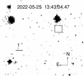
(a) GWAC image before trigger time T0

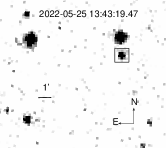
(b) GWAC image at trigger time T0

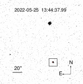
(c) F60A image

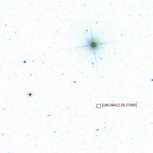
(d) SDSS image

Figure 1: Finding charts for GWAC220525A detected by GWAC,F60A and SDSS DR14. The localization of the flare is marked with a black box in each panels. Panel (a) and (b): GWAC images labeled with the universal time, which were before and near the peak of the event, respectively. The upper is North and the left is EAST. Panel (c): One image obtained by F60A, 79 seconds after the trigger time. The universe time for the measurement is also labeled. Panel (d): reference image derived from the SDSS DR13 survey for a comparison.

3.3 Photometry by LCOGT

The follow-up photometries were performed by Las Cumbres Observatory Global Telescope (LCOGT) (Brown et al., 2013) with three runs from May 25 to 27. 20 $R$-band frames were obtained in total. The exposure time of each image was set to be 300 seconds, which is determined from the brightness estimated from the trend of the brightness estimated from the measurements by both F60A and Xinglong 2.16m telescopes, and the limiting magnitude of the LCOGT telescopes. The correction of bias, dark and flat-field was carried-out with the IRAF software. The astrometric calibration was performed with the Astronomey.net (Lang et al., 2010). The flux calibration was also performed with the same manner adopted for the Xinglong 2.16m and F60A observations. The source is clear detected by stacking the images on each night.

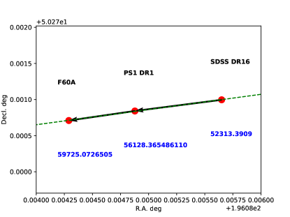
Figure 2: The celestial coordinates derived from SDSS DR16, Panstarrs DR1 and F60A (this work) are plotted by the red circles. The green dashed line and thick black arrows mark the locus on the sky by a linear fitting. The corresponding modified Julian days are labeled in blue. The values of the proper motion are deduced to be $\mu_{\text{RA}}=-241$ and $\mu_{\text{Dec}}=-50\ \mathrm{mas\ yr^{-1}}$, with an maximum of uncertainties of 10%.

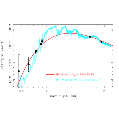
Figure 3: Spectral energy distribution for the source at the quiescent state. The data shown by the black circles are derived from the public archive (WISE, PanStarrs and SDSS surveys, Table 1 in this work). The red and cyan curves show the best-fit blackbody spectrum with a temperature of $1900\pm 50$K and BT-Setti model atmosphere with a temperature of $2200\pm 50$K, repsectively

4 Result

4.1 The quiescent counterpart and the nature of the event

With the astrometry, we cross-match the source with the existing survey catalogs through the VizieR Service. Only one source, hereafter named SDSS J1304 for short, can be founded in SDSS (York et al., 2000), Wide field Infrared Survey Explorer (WISE) (Wright et al., 2010), PanSTARRS DR1 catalog (PS1) (Chambers et al., 2016) within a search radius of 4 arcseconds. No any counterparts can be found at other catalog including Gaia catalog (Gaia Collaboration et al., 2018). The queried key parameters are presented in Table.LABEL:Survey. We plot the celestial coordinates measured by F60A, SDSS and PanStarrs together in Figure.2, which shows an evident proper motion in the past $\sim$20 years. The values of the proper motions are deduced to be $\mu_{\text{RA}}=-241$ and $\mu_{\text{Dec}}=-50\ \mathrm{mas\ yr^{-1}}$. The uncertainties of the proper motions estimated above shall be less than 10% considering the uncertainties of localization and the observation time for the measurements.

All magnitudes in Table.LABEL:Survey are converted to flux density, and the spectral energy distribution (SED) in the quiescent state is built and displayed in Figure.3. The SED is modeled with a black body (BB) spectrum and the BT-Settl model atmospheres available for stars, BDs and planets (Allard, 2014) by a $\chi^{2}$ minimization. The reduced $\chi^{2}$ is 0.90 and 1.18 for the blackbody and BT-Settl model, respectively. Both best-fit models are overplotted in Figure 3. The effective temperature $T_{\text{eff}}$ is obtained to be $1900\pm 25$K for the blackbody model and $2200\pm 50$K for the BT-Settl model. The latter temperature is adopted in this study, which corresponds to a spectral type of M9-L1 according to the relationship between $T_{\text{eff}}$ and the spectral type for low-mass stars (Filippazzo et al., 2015). We take L0 as its spectral type for the following analysis.

Due to its faintness, there is no any reported parallax about the distance of SDSS J1304. Based on the relation between absolution magnitude $M_{\text{W2}}$ and spectral type (Filippazzo et al., 2015), $M_{\text{W2}}\sim 10.0$ mag is obtained. With the distance modulus of 4.622, the distance of the source from us could be deduced to be $d=84\pm 5$ pc after taking the uncertainties of the relation into account.

Taking the first detection by the GWAC is at the peak of the flare (see Section 4.2), the flare amplitudes are calculated to be $\Delta V=-11.2$ mag and $\Delta R=-8.6$ mag by assuming a balckbody emission with a temperature of $\sim 10^{4}$K (Kowalski et al., 2013; Markus & Zhilyaev, 2022) at the peak. With the transparent curves and the zero points of individual filter, the quiescent emission level in $V-$ and $R-$bands used in the calculation is estimated to be $V_{\mathrm{q}}=25.5\pm 0.1$ mag and $R_{\mathrm{q}}=22.9\pm 0.1$ mag, respectively, by an integration of the best-fit BT-Settl model shown in Figure.3.

The two spectra obtained by the 2.16m telescope at the end of the gradual decay phase (see Figure.5 for the details) are displayed in Figure.4. Both spectra show emission lines of $\mathrm{H\alpha}$, $\mathrm{H\beta}$, and He 1$\lambda 5876$, which are commonly detected during a dMe’s flare (Kowalski et al., 2013) and considered to be associated with chromospheric activity. This result suggests that this kind of activities also take place in the BD studied here. We measure the flux of $\mathrm{H\alpha}$ and $\mathrm{H\beta}$ emission lines by a direct integration within the wavelength region 6544-6576Å and 4850-4874Å, respectively. The measured fluxes, along with the uncertainties, are listed in Table.LABEL:spec_line. Both spectra return a Balmer decrement of $\mathrm{H\alpha/H\beta}\approx 1.3$. This decrement can be understood by an emission from an optically thick plasma with a temperature around 5000K according to the local thermal equilibrium calculation (Stelzer et al., 2012).

Figure 4: The two spectra obtained by the 2.16 m telescope at Xinglong Observatory, China, during the gradual decay phase. The observations started at 41 min after the event. #1 is the first spectrum with an exposure time of 600 sec. and #2 show the second spectrum with an exposure time of 20 min. Emission line features are labeled in the figure, which confirms a high chromospheric activity of the source.

Table 1: Properties of SDSS J1304 (the quiescent counterpart of GWAC 220525A) extracted from various surveys. "Offset" means the angular distance from the position given by the survey to the one measured by the F60A.

Parameter	unit	Value
(1)	(2)	(3)
SDSS J130420.55+501615.5
(Ahumada et al., 2020)
R.A.	degree	196.085650
Decl.	degree	+50.270997d
$u$	mag	$24.847\pm 0.652$
$g$	mag	$25.023\pm 0.473$
$r$	mag	$23.714\pm 0.344$
$i$	mag	$21.083\pm 0.064$
$z$	mag	$19.229\pm 0.045$
JD	day	2452313.3909
Offset	arcsec	1.434
Pan-Starrs DR1 (168321960847785676)
(Chambers et al., 2016)
R.A.	degree	196.084877950
Decl.	degree	+50.270842040d
$i$	mag	$21.1139\pm 0.0266$
$z$	mag	$19.5545\pm 0.0327$
$y$	mag	$18.6101\pm 0.0274$
JD	day	2456128.365486110
Offset	arcsec	3.295
WISE J130420.42+501615.1
(Cutri et al., 2013)
R.A.	degree	196.085124
Decl.	degree	+50.270881
$W1$	mag	$14.869\pm 0.031$
$W2$	mag	$14.622\pm 0.05$
Offset	arcsec	1.870

Table 2: Emission line measurements of the spectra of GWAC 220525A displayed in the Figure.4. The emission flux is in the unit of ($\mathrm{10^{-15}\,erg\,s^{-1}\,cm^{-2})}$

Line	Flux(#1)	Flux(#2)
(1)	(2)	(3)
$\mathrm{H\alpha}$	8.1$\pm$0.2	4.5$\pm$0.1
$\mathrm{H\beta}$	6.1$\pm$0.4	3.4$\pm$0.6

Table 3: Fitted parameters of GWAC 220525A used in Equation.1.

$k_{1}$	0.715$\pm$0.001
$\alpha_{1}$	0.767$\pm$0.001
$k_{2}$	0.255$\pm$0.0002
$\alpha_{2}$	0.148$\pm$0.0002
$k_{3}$	0.0409$\pm$0.00003
$\alpha_{3}$	0.0251$\pm$0.00007

4.2 Optical light curve

The $R-$band light curve built from all the measurements from GWAC, F60A, 2.16m and LCOGT telescopes is ploted in Figure.5. We argue that the first detection of the flare by GWAC is close to the peak of the light curve, both because of the non-detection in the frame taken before the the first detection and because the first detection of the flare is the brightest in the light curve. The missing of the rising phase could be resulted from either a very fast energy release or the limited detection ability of the GWAC. Given the detection limit and survey cadence, the flare brighten by 1.5 magnitude in 15 seconds near the peak in the $R-$band.

By following our previous studies (Xin et al., 2021; Wang et al., 2021, 2022), a sum of a set of exponential functions is adopted to describe the decaying phase:

$$\frac{F_{\text{decay}}}{F_{\text{amp}}}=\sum_{i=1}^{n}k_{i}e^{-\alpha_{i}t}$$ (1)

where $F_{\text{decay}}$ is the flux during the decay phase, and $F_{\text{amp}}$ the amplitude flux of the flare which is determined at the peak time. $\alpha$ is the decaying slope. $n$ stands for the number of the components which is needed to account for the behavior of the light curve during the decaying phase, and $k$ is the amplitude of each component. In GWAC 220525A, our inspection by eyes shows that there are four measurements deviating the expected exponential decay at the end of the light curve (i.e., $\sim 10^{4}$ seconds since the peak). However, considering that the brightness derived from the four measurements is quite close to the quiescent level, we do not include them in our light-curve fitting and analysis. Briefly speaking, three exponential components are required to reproduce the observed light curve. In the light-curve fitting, $F_{\mathrm{amp}}$ is fixed to be 2788.97, and a bayesian information criterion (BIC) is adopted to test weather the fitting result by the model is over-fitted The best-fit model associated with a resulted $\chi^{2}=95.2$ with a degree of freedom of 28 is overplotted in Figure 5. Table.LABEL:fitting_parameters summarizes the fitted parameters of the three components.

4.3 Energy budget

Following the approach adopted in previous studies (Kowalski et al., 2013; Xin et al., 2021), the total energy $E_{R}$ in the $R$-band can be estimated by the formula $E_{R}=4\pi r^{2}\times F_{R,\mathrm{q}}\times ED$, where the quiescent flux $F_{R,\mathrm{q}}=2.4\times 10^{-15}$ erg cm^-2 s^-1, and the distance is $r=84$ pc. The equivalent duration $ED$ of a flare is defined to be the time needed to emit all the flare energy at a quiescent flux level (Kowalski et al., 2013). By integrating the modeled light curve over the range from the start to the end of the flare, $ED$ is estimated to be $\sim 5.17\times 10^{5}$ seconds, or 143.6829 hours. The energy $E_{R}$ is therefore evaluated to be $(1.07\pm 0.1)\times 10^{33}$ ergs. Strictly speaking, the method adopted here to estimate energy is only valid for the case in which the flare spectrum is same to the one in the quiescent state. Although this requirement is not fully consistent with fact (Xin et al., 2021), the resulted systematic on the energy due is only $\sim 8\%$ according to our experience. The bolometric energy is $(6.4\pm 0.7)\times 10^{33}$ ergs by assuming the temperature of the flare at the peak time is $10^{4}$K (Kowalski et al., 2013). The fractions of the emitted energy are: 23%, 42% and 35% in the impulsive-, gradual-, and shallow-decay phases, respectively.

4.4 Constraints on magnetic field

The maximum of the vertical magnetic field $B_{z}^{\mathrm{max}}$ can be estimated by the relations given in (Aulanier et al., 2013)

$$E_{\mathrm{bol}}=0.5\times 10^{32}\bigg{(}\frac{B_{z}^{\mathrm{max}}}{1000\mathrm{G}}\bigg{)}^{2}\bigg{(}\frac{L^{\mathrm{bipole}}}{50\mathrm{Mm}}\bigg{)}^{2}\ \mathrm{erg}$$ (2)

where $E_{\mathrm{bol}}$ and $L^{\mathrm{bipole}}$ is the bolometric flare energy and the linear separation between bipoles, respectively. The energy released for GWAC220525A returns a magnetic field about 1.3 kG, when the $L^{\mathrm{bipole}}$ is taken as the maximum distance $\pi R$, where the radius $R$=0.1$R_{\odot}$ is taken as a typical radius of a L0 type star. A kiloguass magnetic field has, in fact, been detected frequently in M to T dwarfs(Hallinan et al., 2008; Morin et al., 2010; Route & Wolszczan, 2016; Kao et al., 2018; Shulyak et al., 2017; Reiners & Basri, 2007; Berdyugina et al., 2017). In addition, a strong field of 3.6–4.7 kG has been inferred in the white-light superflare of a M9-type star detected by the GWAC (i.e., GWAC 181229A(Xin et al., 2021)).

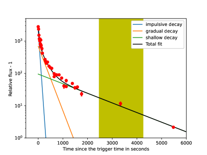
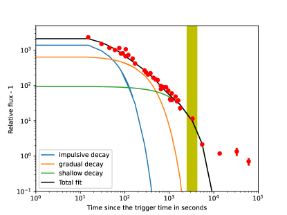
Figure 5: The $R$-band light curve of GWAC 220525A observed by GWAC, F60A, Xinglong 2.16m, and LCOGT telescopes and its modeling. X-axis is the seconds since the trigger time given by the GWAC. Y-aix is the flaring flux normalized by the quiescent flux level. The last four points are quite close to the quiescent flux level, which are not included in the light-curve fitting after taking their uncertainties into account. The best-fit model and the three exponential components are overplotted by the solid lines in different colors. The vertical shadowed region from bottom to top marks the epoch when the two spectra were obtained by the Xinglong 2.16m telescope. The upper panel is the zoomed bottom panel without the display of the measurements after 6000 seconds for the clarity of the modeling during the early phase. The y-axis for the upper panel is in the linear scale while the y-axis for the bottom panel is in the Logarithmic scale.

5 Discussion and conclusion

We here present a powerful white-light flare GWAC 220525A from a L0 star triggerred by the GWAC intense observations at a 15-second short cadence. This is the second white-light stellar flare of very high amplitude ($\Delta R=-8.6$ mag or $\Delta V=-11.2$ mag) and large energy release of an ultra-cool star independently detected by GWAC since 2018. The amplitude of GWAC 220525A is comparable with those previously reported in ultra-cool stars, such as the GWAC 181229A from a M9 star with $\Delta R=-9.5$ mag (Xin et al., 2021), the powerful stellar flares from an early L dwarf ASASSN-16ae (Schmidt et al., 2016) with $\Delta V<-11$ mag, L1 dwarf J005406.55-003101.8 with $\Delta V\sim-8$ mag (Gizis et al., 2017), ASASSN-18di with $\Delta V=-9.8$ mag (Rodríguez et al., 2018)，L2 dwarf ULAS J224940.13-011236.9 with $\Delta V\sim-10$ mag (Jackman et al., 2019), and a superflare with the largest amplitude of $\sim 6.3$ mag detected from Kepler/K2 mission on a L5 dwarf (Paudel et al., 2020) .

5.1 Detection probability of the rare events

The cumulative flare frequency $\nu$ is related with energy $E$ as $\log{\nu}=\alpha+\beta\times\log(E_{32})$ (Lacy, Moffett, & Evans, 1976) , where $\nu$ and $E_{32}$ are in unit of $\mathrm{day^{-1}}$ and $1\times 10^{32}$ erg, respectively. $\alpha$ and $\beta$ are the normalization and slope, respectively. There is evidence that the values of $\beta$ are similar with each others between BDs, the Sun, and other stars, but the normalization parameter is different (Gizis et al., 2013, 2017). However, other studies presented that the slopes are much shallower in cooler stars (Paudel et al., 2018, 2020). Based on $\alpha=-1.35\pm 0.06$ and $\beta=-0.59\pm 0.09$, which is derived from the flares in the energy range between $10^{31}$ and $2\times 10^{32}$ erg in L1 dwarf W1906+40 (Gizis et al., 2013), the rate for GWAC 220525A is predicted to be about 1.45 per year for a flare with energy larger than $6\times 10^{33}$ erg. One has to be caution that this result is sensitive to the parameters we used, which might be not the fact for the source studied in this work.

The detection limit of the GWAC is typical of 15.0 mag in the $R-$band, which means that there is a gap from the detection ability to the maximum brightness of GWAC 220525A for about 1.6 magnitudes. This difference in magnitude corresponds to an energy difference of 4.3 times, which means that only the flares from this dwarf with an energy larger than $\sim 1.4\times 10^{33}$ erg could be detected by the GWAC single images. It therefore results in a detection rate of about 3.44 per year, which is comparable with the estimates of the occurrence rates on the L dwarfs(Paudel et al., 2020), i.e., evergy 2.4 yr for a superflare with energy of $10^{33}$ erg, and every 7.9 yr for a superflare of energy of $10^{34}$ erg. Actually, we have carried out an off-line search of any other flares from this source in the GWAC achieved data obtained from Jan. 2018 to June 2022. In total, we searched 92,161 images. The exposure time for each frame has been fixed to be 10 seconds in our survey, corresponding to a total effective observation time of 256 hours for this field. Only the flare GWAC 220525A was detected in our off-line search. Regardless of the variation of the detection ability during these observations, the detection possibilities of such rare event from this source shall be less than 0.0039 per hour. This non-detection of other superflares supports the low flare rate estimated from the L1 dwarf W1906+40 (Gizis et al., 2013). More monitor needs to be performed to confirm the above estimation.

5.2 Complex of light curve and the configuration of magnetic fields

The light curve of the superflare in GWAC 220525A shows several features which make its decay deviates from an exponential shape. Several components are needed to model the whole shape of the light curve. The continuous cooling of the flaring plasma is interrupted obviously in this event, suggesting that the whole flare originates from multiple active regions. These results suggest that a complex structure of the flare with several loops superimposed consecutively, rather than a single loop(Fletcher et al., 2011).

The multiple phases in the light curve could reflect an evolution of the configuration of the magnetic fields in the corona. During the impulsive phase of GWAC 220525A, the emitted energy is only 23% of the total energy. The dominated energy is released in the later phases. For the gradual phase in this work, the energy faction is up to 42%, indicating new powerful magnetic reconnection occures continuously as the flare arcade caused by the chromospheric evaporation effect in the hot plasma in the framework of the “CSHKP model” (Carmichael, 1964; Sturrock, 1966; Hirayama, 1974; Kopp & Pneuman, 1976). In the current event, an additional decay phase with a much shallower decay index and an energy faction of about 35% is detected after the gradual phase. This kind of component is also detected in other superflare GWAC 181229A (Xin et al., 2021). This additional energy could be generated from an ongoing slow magnetic reconnection and its associated heating (MacCombie & Rust, 1979; Forbes, Malherbe, & Priest, 1989), either above the flare arcade, or conceivably between individual tangled strands of the arcade as they shrink down (Fletcher et al., 2011).

5.3 The possible accompanying CME

Many observations present that more powerful a solar flare, more intense the associated coronal mass ejections (CME) will be (Yashiro et al., 2008; Aarnio et al., 2011; Webb & Howard, 2012; Aarnio, Matt, & Stassun, 2012). This linkage might be valid for the stellar flares (Moschou et al., 2019). A few CME candidates accompanying by the stellar flares have been reported in previous studies (Houdebine, Foing, & Rodono, 1990; Koller et al., 2021; Wang et al., 2021; Chen et al., 2022). A superflare such as reported in this work is expected to be associated with a powerful CME, though there are some debates on the possible suppression on the CME in late M or cooler stars (Alvarado-Gómez et al., 2018; Fraschetti et al., 2019). Considering the habitable zone of a L0 BD is located at $\sim$0.07 AU from the host (Shields, Ballard, & Johnson, 2016), the possible CME, UV emission and high energy particles associated with the superflare would have very heavy impacts not only on the fully co-evolved atmosphere but also on the life (Cherenkov et al., 2017; Schwieterman et al., 2018) on the planets if existing around this dwarf.

Unfortunately, the grism G8 with a spectral resolution of $\sim 2$Å was not available for the Xinglong 2.16m telescope on the night. The low spectral resolution ($\sim 10$Å) of the grism G4 we used does not allow us to detect a possible CME as performed in our previous observations (Wang et al., 2022), unless the velocity of the outflow along the line-of-sight is higher than 1300 $\mathrm{km\ s^{-1}}$.

5.4 Possible "Frog" in time-domain astronomy

The era of time-domain astronomy has been coming. Various facilities with wide FoV in the word-wide are built to discover the counterparts associated to the gravitational wave, gamma-ray burst, fast radio burst, shock break-out emission from supernove, and other cosmic violent explosions. Among these activities, it is no doubt a tough task to identify an optical counterpart of an event with a poor localization (Abbott et al., 2020), such as a gravitational wave event. A localization with an uncertainty of hundreds to thousands degrees (Abbott et al., 2017) makes it not realtise to have intense and deep search for most of facilities in the worldwide if more sky-maps are intent to be covered(Turpin et al., 2020; Frostig et al., 2022). A high-amplitude stellar flare with a rapid decay slope from a very faint dwarf such as GWAC 220525A could make it a false-positive for these cosmic event. For example, the counterpart of this flare is estimated at a distance of 84 pc. If it was more distant from us, ten times more as an instance, the peak magnitude of the flare and the quiescent magnitude would be 18.5 mag and $\sim 28.0$ mag, respectively. On the one hand, a stellar flare with such "bright" peak could be detectable by lots of one meter class telescopes during their day-scale cadence surveys. However, since the fast decay after the peak, it is hard to obtain a spectrum before the end of the event due to a possible long-time delay from the discovery to the follow-ups after its successful identification. On the other hand, at the quiescent state, the counterpart could not be detectable for most of telescopes.

Overall, the characteristics of a bright peak, a fast decay and a very faint counterpart at the quiescent state would result in an incorrect identification by treating a stellar flare as the best candidates of the cosmic event with a bad localization. Highly intense monitor of millions of stars for their activities would be helpful to flag these sources, and a fast spectrum even with a low-resolution at the early phase after an event could provide a very essential clue on its nature.

DATA AVAILABILITY

The datasets generated during and/or analysed during the current study are available from the corresponding author on reasonable request.

References

- Aarnio et al. (2011) Aarnio A. N., Stassun K. G., Hughes W. J., McGregor S. L., 2011, SoPh, 268, 195. doi:10.1007/s11207-010-9672-7
- Aarnio, Matt, & Stassun (2012) Aarnio A. N., Matt S. P., Stassun K. G., 2012, ApJ, 760, 9. doi:10.1088/0004-637X/760/1/9
- Abbott et al. (2017) Abbott B. P., Abbott R., Abbott T. D., Acernese F., Ackley K., Adams C., Adams T., et al., 2017, PhRvL, 119, 161101. doi:10.1103/PhysRevLett.119.161101
- Abbott et al. (2020) Abbott B. P., Abbott R., Abbott T. D., Abraham S., Acernese F., Ackley K., Adams C., et al., 2020, LRR, 23, 3. doi:10.1007/s41114-020-00026-9
- Aberasturi, Solano, & Martín (2011) Aberasturi M., Solano E., Martín E. L., 2011, A&A, 534, L7. doi:10.1051/0004-6361/201117822
- Ahumada et al. (2020) Ahumada R., Allende Prieto C., Almeida A., Anders F., Anderson S. F., Andrews B. H., Anguiano B., et al., 2020, ApJS, 249, 3. doi:10.3847/1538-4365/ab929e
- Allard (2014) Allard F., 2014, IAUS, 299, 271. doi:10.1017/S1743921313008545
- Alvarado-Gómez et al. (2018) Alvarado-Gómez J. D., Drake J. J., Cohen O., Moschou S. P., Garraffo C., 2018, ApJ, 862, 93. doi:10.3847/1538-4357/aacb7f
- Aulanier et al. (2013) Aulanier G., Démoulin P., Schrijver C. J., Janvier M., Pariat E., Schmieder B., 2013, A&A, 549, A66. doi:10.1051/0004-6361/201220406
- Baraffe et al. (2015) Baraffe I., Homeier D., Allard F., Chabrier G., 2015, A&A, 577, A42. doi:10.1051/0004-6361/201425481
- Berdyugina et al. (2017) Berdyugina S. V., Harrington D. M., Kuzmychov O., Kuhn J. R., Hallinan G., Kowalski A. F., Hawley S. L., 2017, ApJ, 847, 61. doi:10.3847/1538-4357/aa866b
- Brown et al. (2013) Brown T. M., Baliber N., Bianco F. B., Bowman M., Burleson B., Conway P., Crellin M., et al., 2013, PASP, 125, 1031. doi:10.1086/673168
- Burrows et al. (2001) Burrows A., Hubbard W. B., Lunine J. I., Liebert J., 2001, RvMP, 73, 719. doi:10.1103/RevModPhys.73.719
- Béjar et al. (2001) Béjar V. J. S., Martín E. L., Zapatero Osorio M. R., Rebolo R., Barrado y Navascués D., Bailer-Jones C. A. L., Mundt R., et al., 2001, ApJ, 556, 830. doi:10.1086/321621
- Carmichael (1964) Carmichael H., 1964, NASSP, 451
- Chabrier et al. (2014) Chabrier G., Johansen A., Janson M., Rafikov R., 2014, prpl.conf, 619. doi:10.2458/azu_uapress_9780816531240-ch027
- Chabrier (2002) Chabrier G., 2002, ApJ, 567, 304. doi:10.1086/324716
- Chabrier (2003) Chabrier G., 2003, PASP, 115, 763. doi:10.1086/376392
- Chambers et al. (2016) Chambers K. C., Magnier E. A., Metcalfe N., Flewelling H. A., Huber M. E., Waters C. Z., Denneau L., et al., 2016, arXiv, arXiv:1612.05560. doi:10.48550/arXiv.1612.05560
- Chen et al. (2022) Chen H., Tian H., Li H., Wang J., Lu H., Xu Y., Hou Z., et al., 2022, ApJ, 933, 92. doi:10.3847/1538-4357/ac739b
- Cherenkov et al. (2017) Cherenkov A., Bisikalo D., Fossati L., Möstl C., 2017, ApJ, 846, 31. doi:10.3847/1538-4357/aa82b2
- Cutri et al. (2013) Cutri R. M., Wright E. L., Conrow T., Fowler J. W., Eisenhardt P. R. M., Grillmair C., Kirkpatrick J. D., et al., 2013, wise.rept
- Fan et al. (2016) Fan Z., Wang H., Jiang X., Wu H., Li H., Huang Y., Xu D., et al., 2016, PASP, 128, 115005. doi:10.1088/1538-3873/128/969/115005
- Filippazzo et al. (2015) Filippazzo J. C., Rice E. L., Faherty J., Cruz K. L., Van Gordon M. M., Looper D. L., 2015, ApJ, 810, 158. doi:10.1088/0004-637X/810/2/158
- Fletcher et al. (2011) Fletcher L., Dennis B. R., Hudson H. S., Krucker S., Phillips K., Veronig A., Battaglia M., et al., 2011, SSRv, 159, 19. doi:10.1007/s11214-010-9701-8
- Forbes, Malherbe, & Priest (1989) Forbes T. G., Malherbe J. M., Priest E. R., 1989, SoPh, 120, 285. doi:10.1007/BF00159881
- Fraschetti et al. (2019) Fraschetti F., Drake J. J., Alvarado-Gómez J. D., Moschou S. P., Garraffo C., Cohen O., 2019, ApJ, 874, 21. doi:10.3847/1538-4357/ab05e4
- Frostig et al. (2022) Frostig D., Biscoveanu S., Mo G., Karambelkar V., Dal Canton T., Chen H.-Y., Kasliwal M., et al., 2022, ApJ, 926, 152. doi:10.3847/1538-4357/ac4508
- Gaia Collaboration et al. (2018) Gaia Collaboration, Brown A. G. A., Vallenari A., Prusti T., de Bruijne J. H. J., Babusiaux C., Bailer-Jones C. A. L., et al., 2018, A&A, 616, A1. doi:10.1051/0004-6361/201833051
- Gizis et al. (2017) Gizis J. E., Paudel R. R., Schmidt S. J., Williams P. K. G., Burgasser A. J., 2017, ApJ, 838, 22. doi:10.3847/1538-4357/aa6197
- Gizis et al. (2017) Gizis J. E., Paudel R. R., Mullan D., Schmidt S. J., Burgasser A. J., Williams P. K. G., 2017, ApJ, 845, 33. doi:10.3847/1538-4357/aa7da0
- Gizis et al. (2013) Gizis J. E., Burgasser A. J., Berger E., Williams P. K. G., Vrba F. J., Cruz K. L., Metchev S., 2013, ApJ, 779, 172. doi:10.1088/0004-637X/779/2/172
- Hallinan et al. (2008) Hallinan G., Antonova A., Doyle J. G., Bourke S., Lane C., Golden A., 2008, ApJ, 684, 644. doi:10.1086/590360
- Han et al. (2021) Han X., Xiao Y., Zhang P., Turpin D., Xin L., Wu C., Cai H., et al., 2021, PASP, 133, 065001. doi:10.1088/1538-3873/abfb4e
- Hazra et al. (2022) Hazra G., Vidotto A. A., Carolan S., Villarreal D’Angelo C., Manchester W., 2022, MNRAS, 509, 5858. doi:10.1093/mnras/stab3271
- Hirayama (1974) Hirayama T., 1974, SoPh, 34, 323. doi:10.1007/BF00153671
- Houdebine, Foing, & Rodono (1990) Houdebine E. R., Foing B. H., Rodono M., 1990, A&A, 238, 249
- Jackman et al. (2019) Jackman J. A. G., Wheatley P. J., Bayliss D., Burleigh M. R., Casewell S. L., Eigmüller P., Goad M. R., et al., 2019, MNRAS, 485, L136. doi:10.1093/mnrasl/slz039
- Kao & Sebastian Pineda (2022) Kao M. M., Sebastian Pineda J., 2022, ApJ, 932, 21. doi:10.3847/1538-4357/ac660b
- Kao et al. (2018) Kao M. M., Hallinan G., Pineda J. S., Stevenson D., Burgasser A., 2018, ApJS, 237, 25. doi:10.3847/1538-4365/aac2d5
- Kirkpatrick (1998) Kirkpatrick J. D., 1998, ASPC, 134, 405
- Koller et al. (2021) Koller F., Leitzinger M., Temmer M., Odert P., Beck P. G., Veronig A., 2021, A&A, 646, A34. doi:10.1051/0004-6361/202039003
- Kopp & Pneuman (1976) Kopp R. A., Pneuman G. W., 1976, SoPh, 50, 85. doi:10.1007/BF00206193
- Kowalski et al. (2013) Kowalski A. F., Hawley S. L., Wisniewski J. P., Osten R. A., Hilton E. J., Holtzman J. A., Schmidt S. J., et al., 2013, ApJS, 207, 15. doi:10.1088/0067-0049/207/1/15
- Lacy, Moffett, & Evans (1976) Lacy C. H., Moffett T. J., Evans D. S., 1976, ApJS, 30, 85. doi:10.1086/190358
- Lang et al. (2010) Lang D., Hogg D. W., Mierle K., Blanton M., Roweis S., 2010, AJ, 139, 1782. doi:10.1088/0004-6256/139/5/1782
- Luhman (2012) Luhman K. L., 2012, ARA&A, 50, 65. doi:10.1146/annurev-astro-081811-125528
- MacCombie & Rust (1979) MacCombie W. J., Rust D. M., 1979, SoPh, 61, 69. doi:10.1007/BF00155447
- Markus & Zhilyaev (2022) Markus Y. S., Zhilyaev B. E., 2022, arXiv, arXiv:2204.11059. doi:10.48550/arXiv.2204.11059
- Morin et al. (2010) Morin J., Donati J.-F., Petit P., Delfosse X., Forveille T., Jardine M. M., 2010, MNRAS, 407, 2269. doi:10.1111/j.1365-2966.2010.17101.x
- Moschou et al. (2019) Moschou S.-P., Drake J. J., Cohen O., Alvarado-Gómez J. D., Garraffo C., Fraschetti F., 2019, ApJ, 877, 105. doi:10.3847/1538-4357/ab1b37
- Mullan & MacDonald (2001) Mullan D. J., MacDonald J., 2001, ApJ, 559, 353. doi:10.1086/322336
- Namekata et al. (2017) Namekata K., Sakaue T., Watanabe K., Asai A., Maehara H., Notsu Y., Notsu S., et al., 2017, ApJ, 851, 91. doi:10.3847/1538-4357/aa9b34
- Paudel et al. (2020) Paudel R. R., Gizis J. E., Mullan D. J., Schmidt S. J., Burgasser A. J., Williams P. K. G., 2020, MNRAS, 494, 5751. doi:10.1093/mnras/staa1137
- Paudel et al. (2018) Paudel R. R., Gizis J. E., Mullan D. J., Schmidt S. J., Burgasser A. J., Williams P. K. G., Berger E., 2018, ApJ, 858, 55. doi:10.3847/1538-4357/aab8fe
- Pineda, Hallinan, & Kao (2017) Pineda J. S., Hallinan G., Kao M. M., 2017, ApJ, 846, 75. doi:10.3847/1538-4357/aa8596
- Reiners & Basri (2007) Reiners A., Basri G., 2007, ApJ, 656, 1121. doi:10.1086/510304
- Reylé (2018) Reylé C., 2018, A&A, 619, L8. doi:10.1051/0004-6361/201834082
- Richey-Yowell et al. (2020) Richey-Yowell T., Kao M. M., Pineda J. S., Shkolnik E. L., Hallinan G., 2020, ApJ, 903, 74. doi:10.3847/1538-4357/abb826
- Rimmer et al. (2018) Rimmer P. B., Xu J., Thompson S. J., Gillen E., Sutherland J. D., Queloz D., 2018, SciA, 4, eaar3302. doi:10.1126/sciadv.aar3302
- Rodríguez et al. (2018) Rodríguez R., Schmidt S. J., Jayasinghe T., Stanek K. Z., Prieto J. L., Shappee B., Kochanek C. S., et al., 2018, RNAAS, 2, 8. doi:10.3847/2515-5172/aabe7d
- Route & Wolszczan (2016) Route M., Wolszczan A., 2016, ApJL, 821, L21. doi:10.3847/2041-8205/821/2/L21
- Sarro et al. (2023) Sarro L. M., Berihuete A., Smart R. L., Reylé C., Barrado D., García-Torres M., Cooper W. J., et al., 2023, A&A, 669, A139. doi:10.1051/0004-6361/202244507
- Schmidt et al. (2016) Schmidt S. J., Shappee B. J., Gagné J., Stanek K. Z., Prieto J. L., Holoien T. W.-S., Kochanek C. S., et al., 2016, ApJL, 828, L22. doi:10.3847/2041-8205/828/2/L22
- Schwieterman et al. (2018) Schwieterman E. W., Kiang N. Y., Parenteau M. N., Harman C. E., DasSarma S., Fisher T. M., Arney G. N., et al., 2018, AsBio, 18, 663. doi:10.1089/ast.2017.1729
- Shields, Ballard, & Johnson (2016) Shields A. L., Ballard S., Johnson J. A., 2016, PhR, 663, 1. doi:10.1016/j.physrep.2016.10.003
- Shulyak et al. (2017) Shulyak D., Reiners A., Engeln A., Malo L., Yadav R., Morin J., Kochukhov O., 2017, NatAs, 1, 0184. doi:10.1038/s41550-017-0184
- Spiegel, Burrows, & Milsom (2011) Spiegel D. S., Burrows A., Milsom J. A., 2011, ApJ, 727, 57. doi:10.1088/0004-637X/727/1/57
- Stelzer et al. (2012) Stelzer B., Alcalá J., Biazzo K., Ercolano B., Crespo-Chacón I., López-Santiago J., Martínez-Arnáiz R., et al., 2012, A&A, 537, A94. doi:10.1051/0004-6361/201118097
- Sturrock (1966) Sturrock P. A., 1966, Natur, 211, 695. doi:10.1038/211695a0
- Tilley et al. (2019) Tilley M. A., Segura A., Meadows V., Hawley S., Davenport J., 2019, AsBio, 19, 64. doi:10.1089/ast.2017.1794
- Turpin et al. (2020) Turpin D., Wu C., Han X.-H., Xin L.-P., Antier S., Leroy N., Cao L., et al., 2020, RAA, 20, 013. doi:10.1088/1674-4527/20/1/13
- Wang et al. (2022) Wang J., Li H. L., Xin L. P., Li G. W., Bai J. Y., Gao C., Ren B., et al., 2022, ApJ, 934, 98. doi:10.3847/1538-4357/ac7a35
- Wang et al. (2021) Wang J., Xin L. P., Li H. L., Li G. W., Sun S. S., Gao C., Han X. H., et al., 2021, ApJ, 916, 92. doi:10.3847/1538-4357/ac096f
- Webb & Howard (2012) Webb D. F., Howard T. A., 2012, LRSP, 9, 3. doi:10.12942/lrsp-2012-3
- Wei et al. (2016) Wei J., Cordier B., Antier S., Antilogus P., Atteia J.-L., Bajat A., Basa S., et al., 2016, arXiv, arXiv:1610.06892. doi:10.48550/arXiv.1610.06892
- Wright et al. (2010) Wright E. L., Eisenhardt P. R. M., Mainzer A. K., Ressler M. E., Cutri R. M., Jarrett T., Kirkpatrick J. D., et al., 2010, AJ, 140, 1868. doi:10.1088/0004-6256/140/6/1868
- Xin et al. (2021) Xin L. P., Li H. L., Wang J., Han X. H., Qiu Y. L., Cai H. B., Niu C. H., et al., 2021, ApJ, 922, 78. doi:10.3847/1538-4357/ac1daf
- Xin et al. (2021) Xin L. P., Li H. L., Wang J., Han X. H., Xu Y., Meng X. M., Cai H. B., et al., 2021, ApJ, 909, 106. doi:10.3847/1538-4357/abdd1b
- Xin et al. (2020) Xin L. P., Han X. H., Wei J. Y., Li L. H., Wang J., Turpin D., Cai H. B., et al., 2020, GCN, 29201
- Xin et al. (2019) Xin L., Han X., Wei J., Wang J., Qiu Y., Wu C., Li H., et al., 2019, mmag.conf, 260. doi:10.26119/SAO.2019.1.35558
- Xu et al. (2020) Xu Y., Xin L. P., Wang J., Han X. H., Qiu Y. L., Huang M. H., Wei J. Y., 2020, PASP, 132, 054502. doi:10.1088/1538-3873/ab7a73
- Yashiro et al. (2008) Yashiro S., Michalek G., Akiyama S., Gopalswamy N., Howard R. A., 2008, ApJ, 673, 1174. doi:10.1086/524927
- York et al. (2000) York D. G., Adelman J., Anderson J. E., Anderson S. F., Annis J., Bahcall N. A., Bakken J. A., et al., 2000, AJ, 120, 1579. doi:10.1086/301513
- Zhang et al. (2017) Zhang Z. H., Homeier D., Pinfield D. J., Lodieu N., Jones H. R. A., Allard F., Pavlenko Y. V., 2017, MNRAS, 468, 261. doi:10.1093/mnras/stx350