Removing supervision in semantic segmentation
with local-global matching and area balancing
Abstract
Removing supervision in semantic segmentation is still tricky. Current approaches can deal with common categorical patterns yet resort to multi-stage architectures. We design a novel end-to-end model leveraging local-global patch matching to predict categories, good localization, area and shape of objects for semantic segmentation. The local-global matching is, in turn, compelled by optimal transport plans fulfilling area constraints nearing a solution for exact shape prediction. Our model attains state-of-the-art in Weakly Supervised Semantic Segmentation, only image-level labels, with 75% mIoU on PascalVOC2012 val set and 46% on MS-COCO2014 val set. Dropping the image-level labels and clustering self-supervised learned features to yield pseudo-multi-level labels, we obtain an unsupervised model for semantic segmentation. We also attain state-of-the-art on Unsupervised Semantic Segmentation with 43.6% mIoU on PascalVOC2012 val set and 19.4% on MS-COCO2014 val set. Code is available at https://github.com/deepplants/PC2M.
1 Introduction
Semantic segmentation is the computational task of discovering object categories in an image, localising them, and predicting their shapes and dimensions. Recent research has successfully proved that weaker or no supervision can overtake demanding pixel supervision.
Weakly Supervised Segmentation methods (WSSS) [64, 18, 11, 60, 44] replace pixel supervision with image-level supervision. The image categories prior define the space of objects. This prior knowledge, combined with the intrinsic ability of deep networks to focus on regions of interest, allows localising class-discriminative regions (CAM [67]). Keeping CAM for proper localisation imposes a tremendous effort to expand and clean CAMs attention maps for improving mask-shapes, such as resorting to affinity net [1, 56, 66, 63].
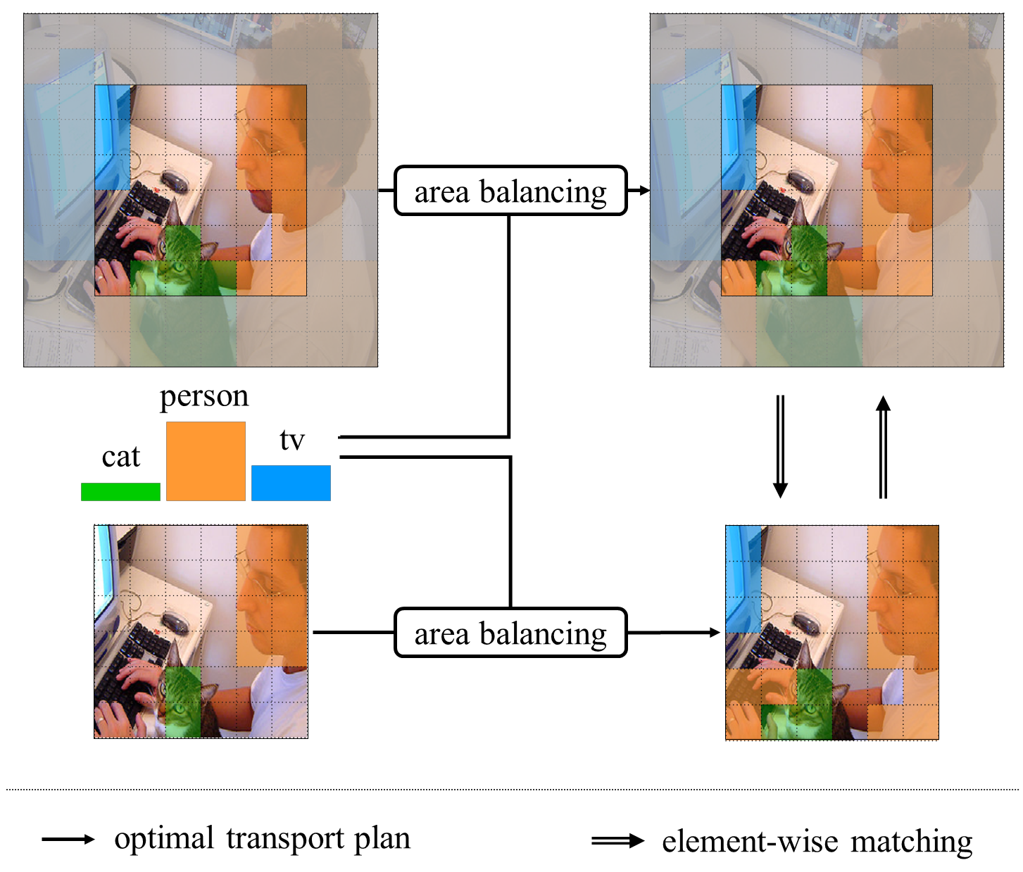

Some methods like AFA [45] and MCTFormer[64] have explored transformers [17], focusing on the use of the class token for uplifting categories to patches, still committing to CAMs for localisation. So far, only [44] have shown that transformers can replace CAM using dense attention for localisation and patch category assignments. CAM ensures sound localisation, although not shape consistency, and to go beyond this bottleneck, these two semantic segmentation properties must be assessed together when supervision is weakened or removed. We take appropriate steps in this direction, nearing the solution to sound localisation and mask shapes. The concept of our work is shown in Figure 1. Here, we present Patch-Class to Masks (PC2M) lifting dimension, hence shape, close to supervised methods.
Unsupervised Semantic Segmentation (USS) methods [23, 38, 25, 21, 12, 53, 35, 69, 24, 58] obtained so far successful results, following the self-supervised representation principles of pulling close similar data and pushing away different ones. Though here, as in dense self-supervised representations, data are not images but pixels, patches, or super-pixels (see, e.g. [55, 33, 39, 40, 62, 57]). These methods leverage pixel similarity and spatial information encoding them into distinctive features corresponding to disjoint categories. Categories discovery relies upon clustering methods to group the learned features into the relevant dataset classes.
Unlike image classification, object detection and recognition, semantic segmentation displays the perception of object states with their semantics, such as their shape, position within the image vantage point, and relative dimension. Dense bottom-up methods such as IIC [23], MaskContrast [53], Leopart [69], and SlotCon [58] focusing on pixel similarities, though producing high-quality masks of object parts, struggle to group consistently discovered parts.
To address this problem we promote our WSSS method to USS, replacing image-level labels with pseudo-labels. The proposed model clusters features self-supervised on ImageNet [46] Our PC2M, illustrated in Figure 2, advances the solution to the unsupervised mask-shape problem by handling the object area estimation for each category.
The main contributions of this work are:
We introduce PC2M an end-to-end network for semantic segmentation supervised with image-level labels. The improvements are due to:
1) PC2M is formed by two branches, one developing on augmentations with image parts and the other with augmentations using most of the image, in so forcing the network to collate local with global information, which is beneficial for grouping object parts;
2) PC2M relative-entropy loss expands with terms contrasting the objects’ area predictions from the two network branches with dense pseudo-labels estimated with transport plans. The transport plans are computed by solving an Optimal Transport (OT) problem [41] with properly generated discrete metrics. An exponential moving average gently drives the network to predict the correct object areas; see the example in Figure 1.
We establish new state-of-the-art performances in WSSS with 76.55% and 75.7% mIoU on PascalVOC2012 [20] train and test set (against the best supervised 89.0% mIoU with DeepLabv3+Xception-65-JFT [7]), and 46.0% on the MS-COCO2014 [34] val set.
We introduce a principled top-down approach to USS. We show that replacing ground-truth labels with self-supervised pseudo-labels leads to a model attaining state-of-the-art performance in USS, with a mIoU of 43.6% on PascalVOC-2012 and 19.42% on MS-COCO2014 val sets. Our top-down method sheds light on the importance of category knowledge. We show that the absence or low precision of contextual information encoded in image-level labels is detrimental to our framework. We argue that improving unsupervised methods for high-quality label extraction is essential for building robust unsupervised segmentation models.
2 Related Works
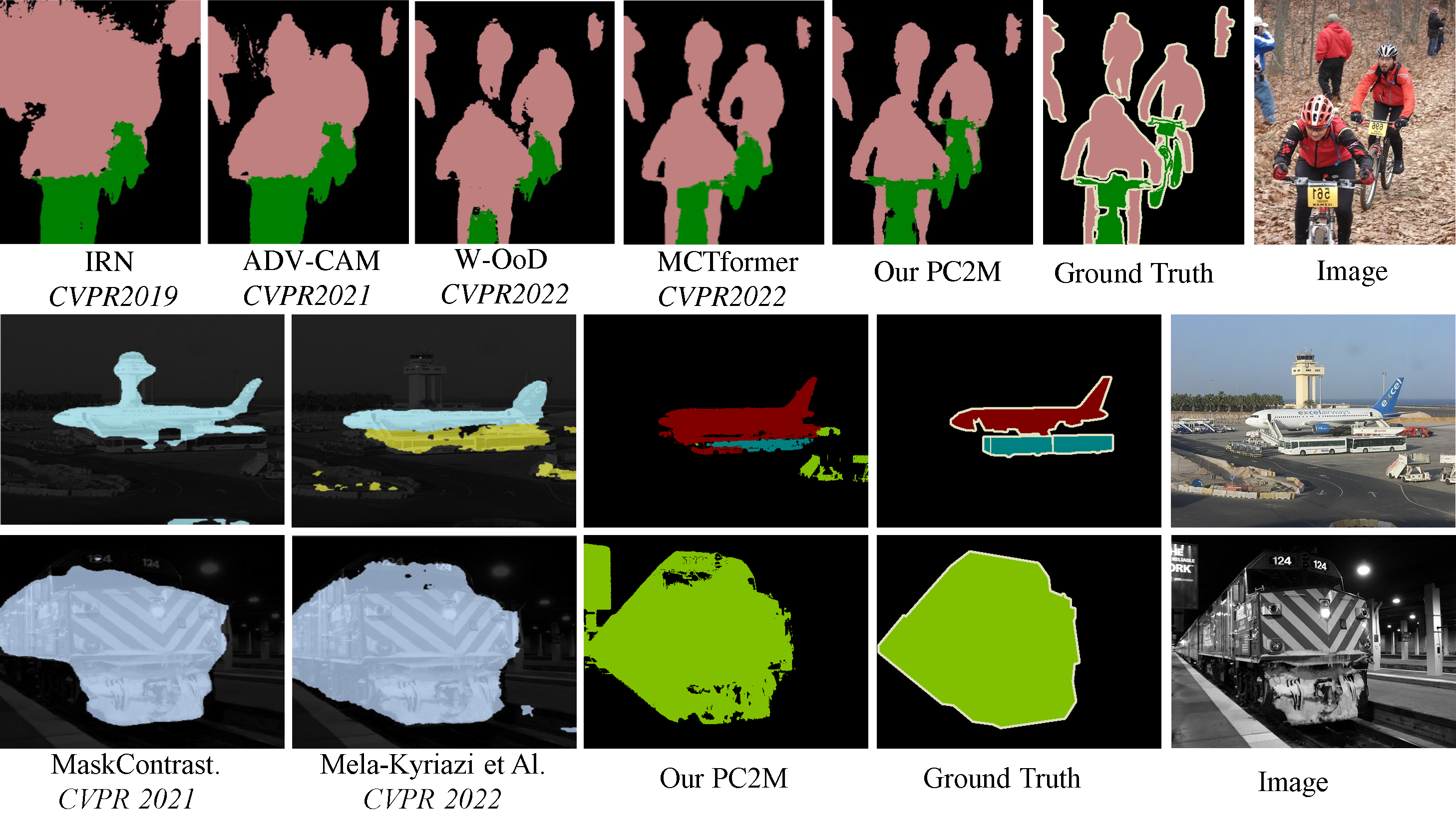
Figure 3 shows the progress of the WSSS and USS research streams in the most recent years.
Weakly supervised semantic segmentation. Recent methods of weakly-supervised segmentation predict pseudo-masks of the object categories with only image-level supervision. After [67] introduced Class Activation Maps (CAM) using a global average pooling layer in their CNN architecture, CAM has been massively used in WSSS [11, 32, 29, 48, 31]. CAM-based methods often rely on mask-refinement procedures to enhance the accuracy of the baseline models, such as dense CRF [27], and affinity maps [1]. Pseudo-mask generation has been contaminated by self-supervised learning in [56] via downstream tasks and transformations, ensuring CAM features equivariance. Contrastive representation learning, for dense pixel embedding, is used in RCA [68], C2AM [61], and in PPC [18]. Lately, transformer-based architectures have gained traction as an alternative to CNN, such as MTCformer [64], AFA [45], and ViT-PCM [44] revealing an improved capacity of ViT in creating complete and well-localised masks. While both [64] and [45] use CAM to refine their pseudo-masks, ViT-PCM predicts categorical distributions at the patch level.
Unsupervised semantic segmentation. USS assigns a semantic label to each image pixel without human annotations, implying the need for multi-label support to discriminate several regions in the image. There are two lines of research on USS. The first is followed by MaskContrast [53], focusing on dense pixel embedding using contrastive learning with initialised saliency maps as priors. MaskContrast is the first method to consider USS. The second line of research is grouping and clustering extended to pixels and patches. Leopart [69] uses DINO features [6] and learns an embedding for grouping similar pixels into object parts. Parts are then clustered according to the foreground and community detection. Clustering object parts incurs the risk of the same parts being assigned to the wrong objects. PiCIE [12] incorporates invariance to photometric and equivariance to geometric transformations. IIC [23] uses mutual information for clustering and applies it to image patches. Similarly, [24] start with classical grouping from OWT-UCM [4], a grouping method that can hardly be leveraged for large-scale datasets. The method of [35] is the first one that elegantly solves the multi-label problem. Indeed, [35] extracts DINO-ViT-Base [6] features to find the image segments by computing the gap between the non-null eigenvalues of the features Laplacian. In our top-down approach we follow a methodology similar to [35], to generate pseudo-labels supervising an end-to-end network for USS.
3 Our Approach
This section presents our method by first discussing the model achieving state-of-the-art semantic segmentation with image-level label supervision. We further show how to expand our framework to unsupervised segmentation.
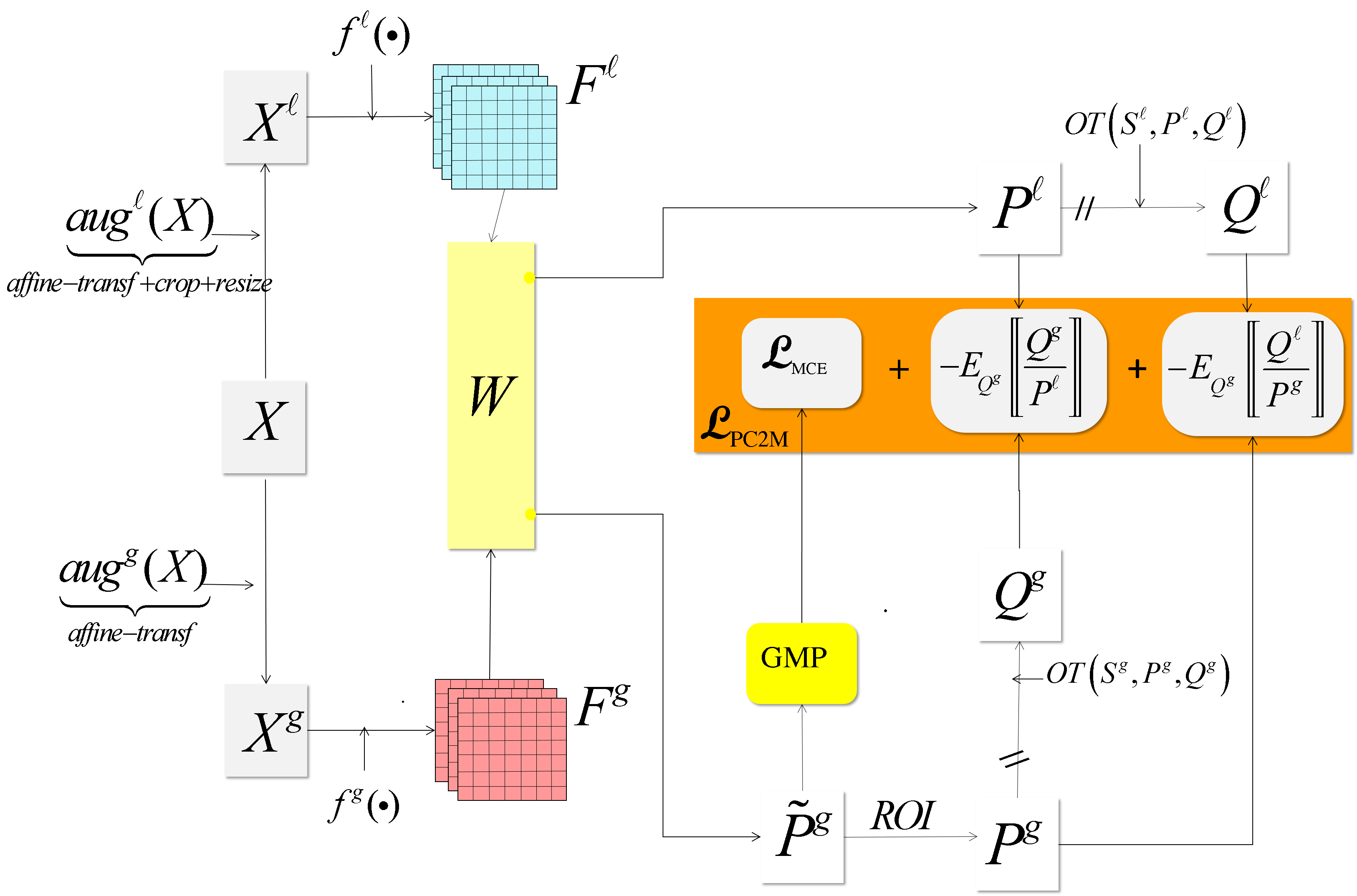
Similarly to [44], which has shown excellent ability in localising class-relevant image segments given image-level supervision, we define a two-branch network based on ViT [17]. By feeding different augmented views (one seizing most of the original image and one randomly cropping parts of it) to the two branches, we elicit representations for global and local views of a particular object category. The pooled predictions of the global branch are contrasted with the ground-truth image-level labels. We use both branches’ un-pooled patch predictions to yield dense pseudo-labels computed with the Sinkhorn-Knopp algorithm [15]. Namely, we formulate an Optimal Transport problem [41] to constrain the dense pseudo-labels to assign each patch to a single class. Additionally, each patch assignment is balanced by the estimated normalised area of each class in the dataset. Since this area is unknown, we begin the training under the hypothesis that each object has an area proportional to the relative frequency of its category and slowly update it with the network empirical estimates. Finally, we set up a contrastive loss between each branch patch prediction and the computed dense pseudo-labels.
3.1 Preliminaries
Let , with , be a specified dataset with class labels , with the cardinality of . In the multi-label segmentation setting . For each input image , we create two views: one global view retaining most of the original image, and a local view obtained by randomly cropping and resizing . The two views are augmented by randomly sampling a transformation from a set that includes jittering and affine transformations.
We consider an encoder as the backbone network indicated by ; although their weights are shared (see Figure 2), we refer to the two branches as and for clarity.
Let with be the number of encoded patches of dimension for a specific augmented view . Let be the number of samples we consider in a batch of each branch . Let and be the two feature matrices of the augmented views conveyed from each branch. Each feature vector , , specifies the feature encoding a patch of a sampled augmented view from branch . The features , are projected on a dense layer with units shared by the two network branches and . The estimated weights are .
is the un-normalised cosine similarity between the features of the encoded -th patch and the class represented by the weight vector , the posterior probability that the patch label is of class is:
| (1) |
which is the -th element of the prediction matrix , . enforces a categorical distribution for each patch : .
Optimization objective We first define the match-loss, given and , as follows:
| (2) |
Here, and are probability matrices with, respectively, marginal distributions , and , generated according to conditions specified in the next section. A stop-gradient operation avoids the gradient back-propagation of the entropy terms. The complete objective is:
Here is the standard multi-label binary cross-entropy loss, as in [44].
3.2 Optimal Transport for computing and
In this section, we describe how we generate the coupling matrices [51] used in the match-loss, with Optimal Transport (OT).
Here is the entropy of a coupling matrix, is a weight of the entropy regularization, , is a cost matrix, and are probability vectors in the probability simplices with and bins, and the polytope
| (4) |
provides the mass conservation criterion [41]. Solutions of the linear program in (3) find a transportation plan of minimal cost such that the marginal distributions of are the discrete measures and . In practice, (3) ensures a unique solution of the OT problem converging to the maximal entropy transport coupling for a small regularisation , see [41, 16].
Using the above results, and given , we define the two couples of probability vectors and , generating the transportation plans and . In the following, the computation of is the same as that of in the two branches; therefore, we drop the superscripts.
Since we interpret as the dense pseudo-labels for a specific algorithm iteration, the specified marginals over the class dimension can be deemed the vector of the normalised areas for each class in the full dataset. Given the image labels, we re-scale the class areas at each iteration to account for the class frequencies in the batch with respect to those in the dataset. Therefore, its exact form is111Each operation is intended element-wise:
| (5) |
Here is the estimated class areas distribution, and are the relative class frequencies in the dataset and in the current batch. is a normalization factor ensuring is a discrete measure. We initialise uniformily as .
At each epoch , is updated offline to the dataset’s current predictions for each with an exponential moving average (EMA). Where the probability density vector of each with respect to class is:
| (6) |
For all in the dataset the update of the -th element of at epoch is:
| (7) |
Here is the unit area momentum rate. For the optimization (3) the solution proposed in [15, 41] finds the optimal by computing two (unknown) scaling variables , such that , with , a Gibbs kernel, and a cost function. Here, to obtain and we define the two kernels to be the predictions and , that is, our cost matrices are, for : . The scaling vectors for and are computed by Sinkhorn’s algorithm presented in [15].
It is easy to see that if for all , with the number of patches in an image, then the Sinkhorn algorithm stops updating, a condition we call convergence for our method. In fact, since , with we have, dropping the superscript :
| (8) |
up to a constant.
On the other hand, the EMA stops updating when for all :
| (9) |
as can be derived from Equation 7. Hence, the network estimated marginal distributions over the class dimensions already match the prescribed distribution . Moreover, the marginal of the network predictions over the patches dimension matches by construction222We further discuss these equalities and convergence in Appendix A.
3.3 Unsupervised Segmentation
We withdraw the image-level labels and compute the pseudo-multi-labels using self-supervised features to make the above method unsupervised. Similar to [47] and [35] we use DINO [6] self-supervised features.
For each image in , split in patches, we construct a graph with vertices and edges where is a self-supervised pre-trained feature extractor and is the pairwise affinity function:
| (10) |
We compute the normalized Laplacian of the graph as , where is the degree matrix and . After calculating the eigendecomposition of the graph Laplacian, the eigenvectors are clustered to obtain homogeneous regions, which are cropped and resized to a standard dimension. For each crop of , we compute its CLS token feature and finally run -means clustering on all the crops in with . The cluster memberships of the crops define the desired pseudo-labels.
4 Experiments
We evaluate the effectiveness of our approach by performing experiments on the single semantic segmentation task but differentiating between two supervision strategies. First, we consider the weakly supervised case, and we further analyse the effectiveness of the unsupervised one.
4.1 Datasets and Metrics
For all experiments, we report the mIoU metric for the semantic segmentation task on PascalVOC2012 [20] (20 classes) augmented with the SBD dataset [22]. We also evaluate our method on MS-COCO2014 [34] (80 classes). We initialize our backbone as a Vision Transformer [17], namely ViT-B/16, with weights pre-trained on ImageNet [46], following [44] for the WSSS task. For unsupervised segmentation, we start from a DINO [6] initialization, similarly to [69, 35].
4.2 Implementation Details
After one warm-up epoch, during which the initialized weights are frozen, we unfreeze the last five layers of the network and train the model on 2 NVIDIA RTX A6000 GPUs. For the PascalVOC2012 dataset, the model has been trained for 45 epochs, with a total training time of 4h 10min, while for MS-COCO2014, the training phase lasted 4h 50min and ran for 10 epochs. We discuss the algorithmic complexity of our method in Appendix C. We use Adam [26] optimizer and scale the initial learning rate by after the warm-up step. At the end of every epoch, we update the target distributions for each class. The algorithm pseudo-code is presented in Appendix B. As specified in Eq. 7, we employ an exponential moving average (EMA). We modulate the EMA update via a momentum parameter and discuss its effects in Section 4.3.
4.3 Ablation Studies
In this paragraph, we investigate the relative importance of the main components of our method by systematically ablating them.
Optimal Transport. During early training phases, the MCE optimisation localises the relevant patches to each category. Though, initially, the actual area estimation is quite inaccurate. A low value of ensures that inaccurate estimations are discarded while encouraging matching predictions to the initial uniform distribution. While training progress, trades off between the current and past estimations. As a consequence of these observations, we set to for all experiments unless explicitly stated. As the network area predictions get more accurate, becomes irrelevant. Indeed, as shown in Figure 6, the EMA update of stops after epochs. In Figure 4 (left), we report the model’s performance as mIoU with varying values for . In practice, the slow EMA update improves mIoU over the frozen uniform distribution case. For higher values of , the network predictions are vulnerable to its own bias favouring the most frequent of categories. Figure 4 (right) shows that large s drive the network to a degenerate solution, exemplified by the entropy dropping to zero. In Table 2, we show that removing the OT step and relying only on global-local correspondence leads to a sharp drop in mIoU accuracy.
Match-loss. We evaluate the importance of trading predictions and transportation plans between the network branches via a cross-entropy loss. In order to do this, we remove the connection between the two branches provided by Equation 2 and minimise the cross-entropy between the predictions of a branch and its transportation plan. In Table 2, we can see a substantial decline of the mIoU accuracy of , which we ascribe to the drop of the local-global correspondence in the loss function.
ViT backbone. In Table 2 a comparison between different ViT architectures [17] performance is presented. While the accuracy of the and model are comparable, there is a drop () for the version of ViT. We deduce that the quality of the extracted features depends weakly on the model size.
| Backbone | OT | Match | Results |
|---|---|---|---|
| ViT-S/16 | ✓ | 35.12 | |
| ✓ | 61.42 | ||
| ✓ | ✓ | 69.05 | |
| ViT-B/8 | ✓ | ✓ | 73.12 |
| ViT-B/16 | ✓ | ✓ | 75.56 |
| ViT-L/16 | ✓ | ✓ | 75.24 |
| Supervision | Method | PascalVOC2012 | COCO2014 |
|---|---|---|---|
| WSSS | val | 75.0 | 46.0 |
| test | 75.7 | ||
| USS | val | 43.6 | 19.55 |
Exploring Different Levels of Supervision. As shown in Table 2 there is a drop of 30 points between weakly supervised and unsupervised mIoU. In this section, we examine how the availability of ground-truth labels influences these results. We randomly replace a fraction of the ground-truth labels for the generated pseudo-labels, using Hungarian matching [28] to map one to the other. In Figure 6, we recognize an initial sharp drop in accuracy with . The drop indicates that the amount of the pseudo-labels strongly influences the model accuracy in this regime; with , there is a smoother accuracy drop, indicating that in this interval, there might be some other component influencing this behaviour.

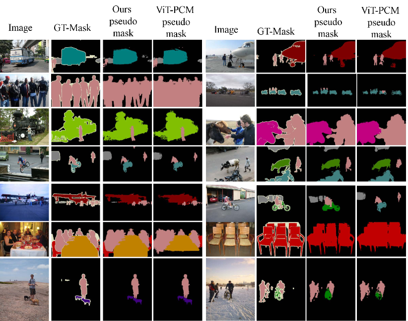
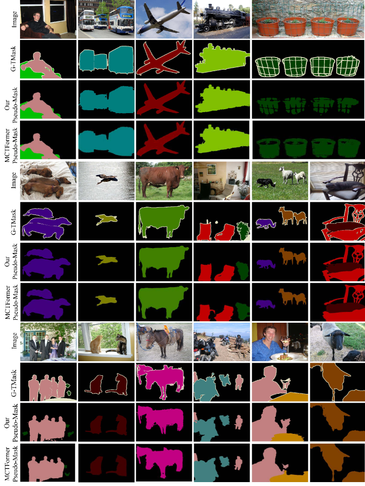
4.4 Qualitative results
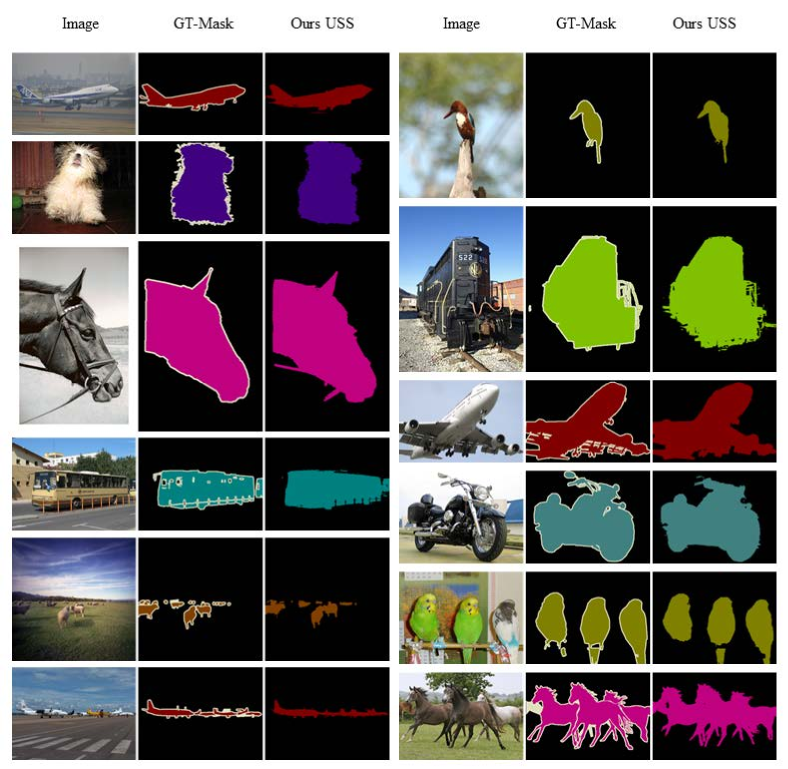
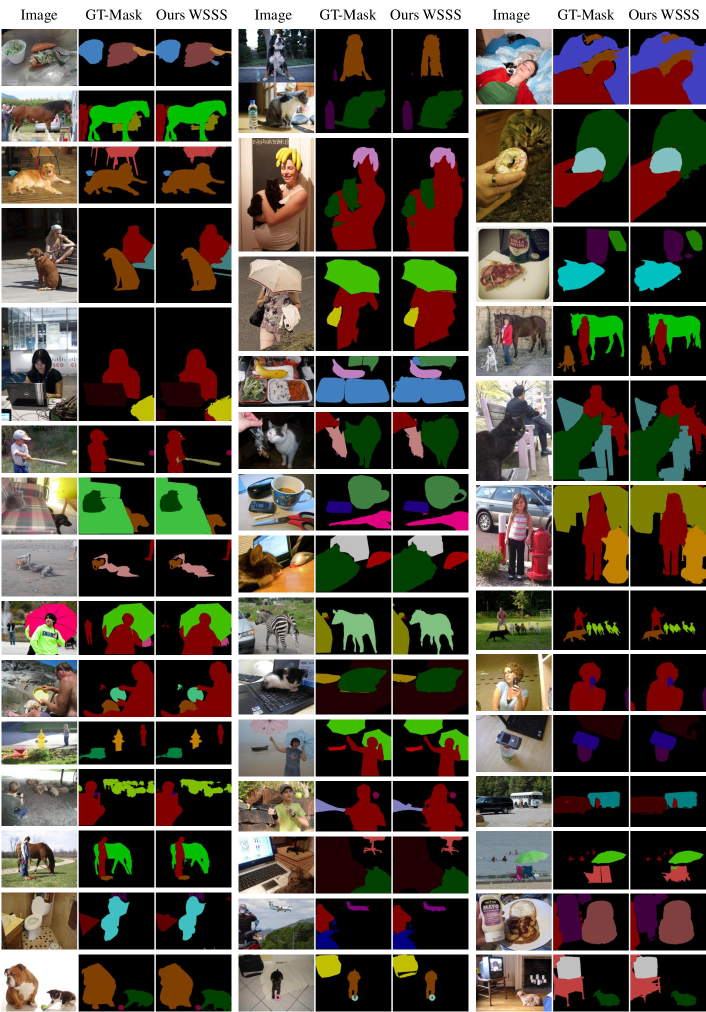
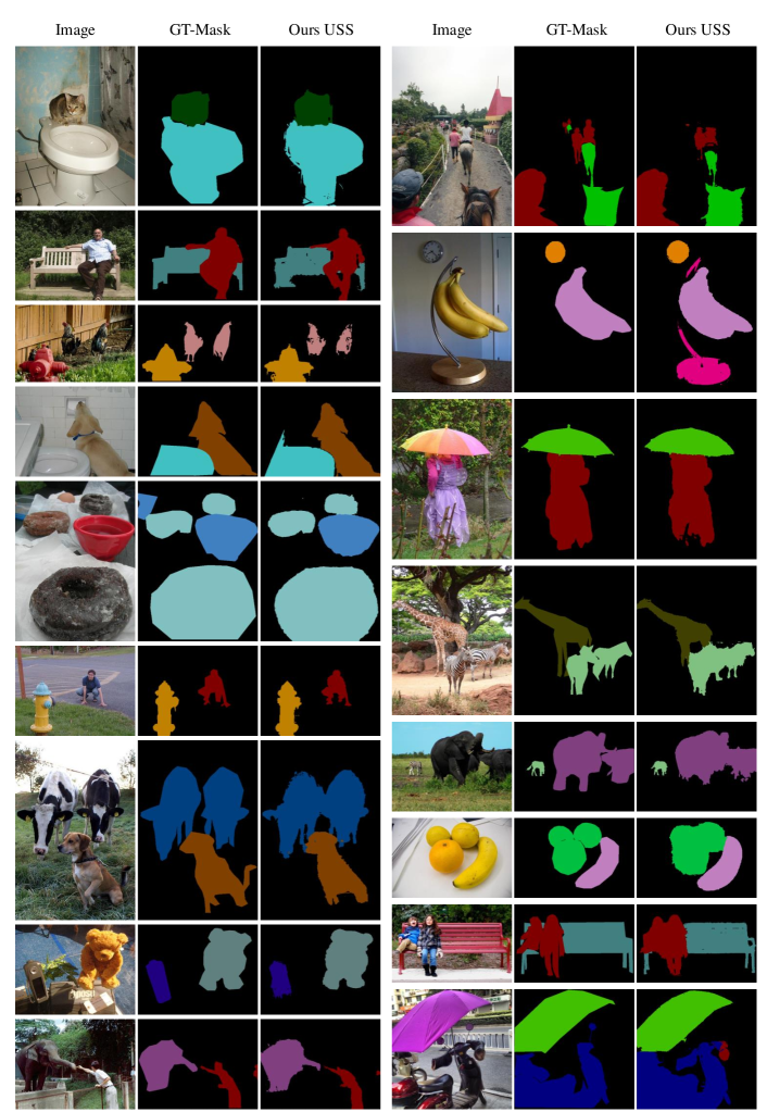
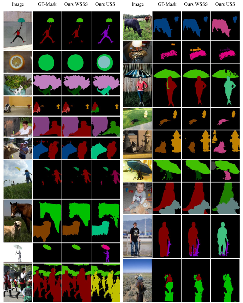
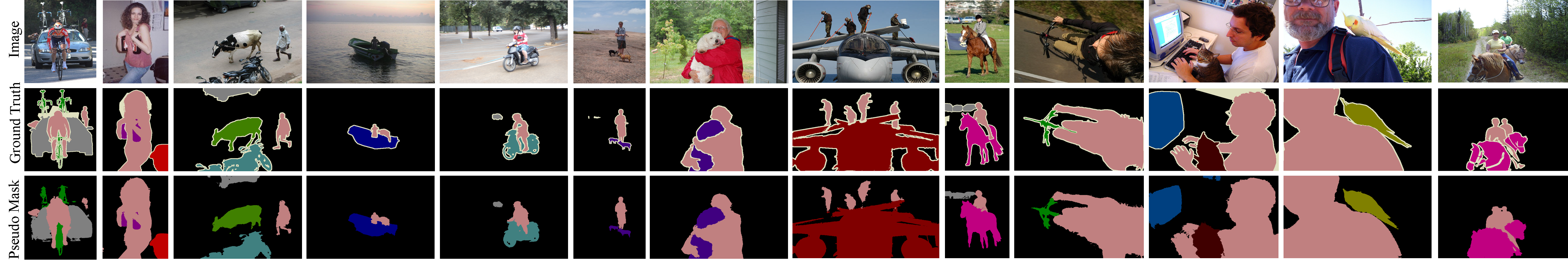
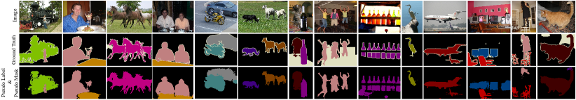
We show our qualitative results in Figures 7 to 9 for the weakly supervised and unsupervised tasks. Note that the white regions in the ground-truth masks are no-class. Our PC2M-generated pseudo-masks exhibit close-to-ground-truth mask shapes and contours. In Appendix E more qualitative results on both WSSS and USS on PascalVOC2012 and on MS-COCO2014 datasets can be found, together with qualitative comparisons to other approaches.
4.5 Comparison to the State of the Art
Weakly supervised semantic segmentation We compare our method with the most recent approaches in the literature (2021-2022) on PascalVOC2012[20], and MS-COCO2014 [34] since mIoU scores steadily grow over time. We have used the same nomenclature of ViT-PCM [44] distinguishing between raw Baseline Pseudo-Masks (BPM) and those refined with CRF [27]. See columns 3-4 of Table 3, where the contribution of CRF is apparent. On validation and test, DeepLab [7] is used to verify the predicted pseudo-masks, often resorting to a different backbone than the one used for predicting the pseudo-masks. Note that, as indicated with the in Tables 3, 4, 5, 7 and 6, we do not train any additional segmentation network to improve generalization, such as DeepLab, nor we use additional forms of supervision, such as saliency maps. Several authors [3, 45, 44] have observed that there is a striking difference between end-to-end networks and multi-stage networks. We can appreciate the disparity by looking at the accuracy jump between Table 3 and Table 4 for some models and the number of parameters used, for example, with Resnet38.
Just a few approaches have been tested on MS-COCO2014, due to the larger number of classes and resources required. Good results are attained by AFA [45], MCTformer[64] (which has an end-to-end version), and ViT-PCM [44], all based on ViT [17]. We also outperform the state-of-the-art on MS-COCO2014.
| Method | Backbone | BPM | BPM+CRF |
|---|---|---|---|
| AdvCAM[31]CVPR’21 | ResNet50 | 55.60 | 62.10 |
| CPN[66]ICCV’21 | ResNet38 | 57.43 | - |
| CSE[29]ICCV’21 | ResNet38 | 56.0 | 62.8 |
| EDAM[59]CVPR’21 | ResNet101 | 52.83 | 58.18 |
| AMR[42] AAAI’22 | Resnet50 | 56.8 | 69.7 |
| MCTformer[64]CVPR’22 | DeiT-S | 61.70 | - |
| PPC[18]CVPR’22 | Resnet38 | 61.50 | 64.00 |
| CLIMS[60]CVPR’22 | Resnet50 | 56.60 | - |
| SIPE[9]CVPR’22 | Resnet50 | 58.60 | 64.70 |
| AdvCAM+W-OoD[32]CVPR’22 | Resnet50 | 59.10 | 65.50 |
| AFA[45]CVPR’22 | MiT-B1 | 63.80 | 66.00 |
| ViT-PCM[44]ECCV’22 | ViT-B/16 | 67.71 | 71.4 |
| Ours⋆ | ViT-B/16 | 75.56 | 76.55 |
| Method | Backbone | Val | Test |
|---|---|---|---|
| AdvCAM[31]CVPR’21 | ResNet50 | 68.1 | 68.0 |
| CPN[66]ICCV’21 | ResNet38 | 67.8 | 68.5 |
| CSE[29]ICCV’21 | ResNet38 | 68.4 | 68.2 |
| EDAM[59]CVPR’21 | ResNet101 | 52.83 | 58.18 |
| AMR[42] AAAI’22 | Resnet101 | 68.8 | 69.1 |
| [54]CVPR’22 | Resnet101 | 66.2 | 66.9 |
| MCTformer[64]CVPR’22 | Resnet38 | 71.9 | 71.6 |
| PPC[18]CVPR’22 | Resnet38 | 72.60 | 73.60 |
| CLIMS[60]CVPR’22 | Resnet50 | 70.4 | 70.0 |
| SIPE[9]CVPR’22 | Resnet101 | 68.8 | 69.7 |
| AdvCAM+W-OoD[32]CVPR’22 | Resnet38 | 70.7 | 70.1 |
| MCIS[50]ECCV’20 | ResNet101 | 66.2 | 66.9 |
| AFA[45]CVPR’22 | MiT-B1 | 66.0 | 66.3 |
| ViT-PCM[44]ECCV’22 | ResNet 101 | 70.3 | 70.9 |
| Ours⋆ | ViT-B/16 | 75.0 | 75.7 |
| Method | Backbone | Val |
|---|---|---|
| RIB[30]Neurips’2021 | R101 | 43.8 |
| MCTformer[64]CVPR’22 | Resnet38 | 42.0 |
| SIPE[9]CVPR’22 | Resnet38 | 43.6 |
| AFA[45]CVPR’22 | MiT-B1 | 38.9 |
| ViT-PCM[44]ECCV’22 | ViT-B/16 | 45.0 |
| Ours⋆ | ViT-B/16 | 46.0 |
| Method | Pretrain Dataset | Backbone | Initial Weights | Val |
|---|---|---|---|---|
| MaskContrast[53]CVPR’2021 | COCO | - | MoCo-v2[10] | 35.0 |
| Leopart[69]CVPR’2022 | COCO | ViT-S/16 | DINO[6] | 41.7 |
| SemSpectral[35]CVPR’2022 | ImageNet | - | DINO[6] | 30.8 |
| HSG[24]CVPR’2022 | COCO | ResNet 50 | - | 41.9 |
| TransFGU[65]ECCV’2022 | ImageNet | ViT-S/8 | DINO[6] | 37.15 |
| Ours⋆ | ImageNet | ViT-B/16 | DINO[6] | 43.6 |
| Method | Pretrain Dataset | Backbone | Initial Weights | Val |
|---|---|---|---|---|
| MaskContrast[53]CVPR’2021 | COCO | - | MoCo-v2[10] | 3.73 |
| TransFGU[65]ECCV’2022 | ImageNet | ViT-S/8 | DINO[6] | 12.69 |
| Ours⋆ | ImageNet | ViT-B/16 | DINO[6] | 19.55 |
Unsupervised semantic segmentation. We compare our method with all available state-of-the-art results on PascalVOC2012 and MS-COCO2014; see Table 6 and Table 7. Initial methods confronted with COCO-stuff [5] and subsets of COCO-stuff due to the difficulty of dealing with the background. The methodology in [53, 35] uses weights from self-supervised representation learning, trained on ImageNet and further applies the unsupervised clustering method. Finally, DeepLab [7] is trained with a backbone pre-trained with self-supervision, and the output is matched with ground-truth labels from the validation set via the Hungarian matching [28]. On the other hand, HSG [24], Leopart[69] and TransFGU[65] evaluate directly on the predicted pseudo-mask. We do not use DeepLab either, outperforming current state-of-the-art; by the way, DeepLab results can be found in the Appendix for completeness.
On MS-COCO2014, our only competitor is TransFGU [65]; the reported results for MaskContrast are from the TransFGU re-implementation with ViT backbone trained by DINO. We improve their methods by 6.86 points in mIoU.
5 Limitations
Our PC2M models a categorical distribution over patches, so using it as a plug-and-play solution in CAM-based methods can be challenging. Indeed, a mapping of the CAM activations to the categorical distribution would be necessary. While for WSSS, the improvement has touched 15 points in mIoU in the last two years, the gap of USS with WSSS is 30 points in mIoU. Knowledge of contextual information is crucial to our top-down framework, and for this reason, it should be improved. Future work requires moving the pseudo labels generation in the loop with the mask prediction, especially caring about multi-labelling.
6 Conclusions
We presented the PC2M that proves excellent performance on semantic segmentation supervised by image-class labels only. We extended the method to unsupervised semantic segmentation by predicting pseudo-labels that can capture the multiplicity of objects in datasets such as PascalVOC2012 and MS-COCO2014. PC2M uses pseudo-labels to predict pseudo-masks. The gap between unsupervised semantic segmentation and the weakly supervised one remains relevant. Nevertheless, the results are promising from the perspective of conjugating the pseudo-labels prediction step with the pseudo-masks one. More details are in the Appendices.
References
- [1] Jiwoon Ahn and Suha Kwak. Learning pixel-level semantic affinity with image-level supervision for weakly supervised semantic segmentation. In CVPR, pages 4981–4990, 2018.
- [2] Jason M. Altschuler, Jonathan Weed, and Philippe Rigollet. Near-linear time approximation algorithms for optimal transport via sinkhorn iteration. CoRR, abs/1705.09634, 2017.
- [3] Nikita Araslanov and Stefan Roth. Single-stage semantic segmentation from image labels. In CVPR, pages 4253–4262, 2020.
- [4] Pablo Arbelaez, Michael Maire, Charless Fowlkes, and Jitendra Malik. From contours to regions: An empirical evaluation. In CVPR, pages 2294–2301. IEEE, 2009.
- [5] Holger Caesar, Jasper Uijlings, and Vittorio Ferrari. Coco-stuff: Thing and stuff classes in context. In CVPR, pages 1209–1218, 2018.
- [6] Mathilde Caron, Hugo Touvron, Ishan Misra, Hervé Jégou, Julien Mairal, Piotr Bojanowski, and Armand Joulin. Emerging properties in self-supervised vision transformers. In ICCV, pages 9650–9660, 2021.
- [7] Liang-Chieh Chen, George Papandreou, Iasonas Kokkinos, Kevin P. Murphy, and Alan Loddon Yuille. Deeplab: Semantic image segmentation with deep convolutional nets, atrous convolution, and fully connected crfs. IEEE TPAMI, 40:834–848, 2018.
- [8] Liang-Chieh Chen, Yukun Zhu, George Papandreou, Florian Schroff, and Hartwig Adam. Encoder-decoder with atrous separable convolution for semantic image segmentation. In ECCV, pages 801–818, 2018.
- [9] Qi Chen, Lingxiao Yang, Jian-Huang Lai, and Xiaohua Xie. Self-supervised image-specific prototype exploration for weakly supervised semantic segmentation. In CVPR, pages 4288–4298, 2022.
- [10] Xinlei Chen, Haoqi Fan, Ross Girshick, and Kaiming He. Improved baselines with momentum contrastive learning. arXiv preprint arXiv:2003.04297, 2020.
- [11] Zhaozheng Chen, Tan Wang, Xiongwei Wu, Xian-Sheng Hua, Hanwang Zhang, and Qianru Sun. Class re-activation maps for weakly-supervised semantic segmentation. In CVPR, pages 969–978, 2022.
- [12] Jang Hyun Cho, Utkarsh Mall, Kavita Bala, and Bharath Hariharan. Picie: Unsupervised semantic segmentation using invariance and equivariance in clustering. In CVPR, pages 16794–16804, 2021.
- [13] Michael B Cohen, Aleksander Madry, Dimitris Tsipras, and Adrian Vladu. Matrix scaling and balancing via box constrained newton’s method and interior point methods. In FOCS, pages 902–913. IEEE, 2017.
- [14] Thomas M. Cover and Joy A. Thomas. Elements of Information Theory 2nd Edition. Wiley-Interscience, 2006.
- [15] Marco Cuturi. Sinkhorn distances: Lightspeed computation of optimal transport. In NeurIPS, volume 26, 2013.
- [16] Marco Cuturi and Gabriel Peyré. Semidual regularized optimal transport. SIAM Review, 60(4):941–965, 2018.
- [17] Alexey Dosovitskiy, Lucas Beyer, Alexander Kolesnikov, Dirk Weissenborn, Xiaohua Zhai, Thomas Unterthiner, Mostafa Dehghani, Matthias Minderer, Georg Heigold, Sylvain Gelly, et al. An image is worth 16x16 words: Transformers for image recognition at scale. ICLR, 2021.
- [18] Ye Du, Zehua Fu, Qingjie Liu, and Yunhong Wang. Weakly supervised semantic segmentation by pixel-to-prototype contrast. In CVPR, pages 4320–4329, 2022.
- [19] Pavel E. Dvurechensky, Alexander V. Gasnikov, and Alexey Kroshnin. Computational optimal transport: Complexity by accelerated gradient descent is better than by sinkhorn’s algorithm. CoRR, abs/1802.04367, 2018.
- [20] Mark Everingham, Luc Van Gool, Christopher KI Williams, John Winn, and Andrew Zisserman. The pascal visual object classes (voc) challenge. IJCV, 88(2):303–338, 2010.
- [21] Robert Harb and Patrick Knöbelreiter. Infoseg: Unsupervised semantic image segmentation with mutual information maximization. In DAGM-GCPR, pages 18–32. Springer, 2021.
- [22] Bharath Hariharan, Pablo Arbeláez, Lubomir Bourdev, Subhransu Maji, and Jitendra Malik. Semantic contours from inverse detectors. In ICCV, pages 991–998. IEEE, 2011.
- [23] Xu Ji, Joao F Henriques, and Andrea Vedaldi. Invariant information clustering for unsupervised image classification and segmentation. In ICCV, pages 9865–9874, 2019.
- [24] Tsung-Wei Ke, Jyh-Jing Hwang, Yunhui Guo, Xudong Wang, and Stella X Yu. Unsupervised hierarchical semantic segmentation with multiview cosegmentation and clustering transformers. In CVPR, pages 2571–2581, 2022.
- [25] Wonjik Kim, Asako Kanezaki, and Masayuki Tanaka. Unsupervised learning of image segmentation based on differentiable feature clustering. IEEE TIP, 29:8055–8068, 2020.
- [26] Diederik P. Kingma and Jimmy Ba. Adam: A method for stochastic optimization. In ICLR, 2015.
- [27] Philipp Krähenbühl and Vladlen Koltun. Efficient inference in fully connected crfs with gaussian edge potentials. NeurIPS, 24, 2011.
- [28] Harold W Kuhn. The hungarian method for the assignment problem. NRLQ, 2(1-2):83–97, 1955.
- [29] Hyeokjun Kweon, Sung-Hoon Yoon, Hyeonseong Kim, Daehee Park, and Kuk-Jin Yoon. Unlocking the potential of ordinary classifier: Class-specific adversarial erasing framework for weakly supervised semantic segmentation. In ICCV, pages 6994–7003, 2021.
- [30] Jungbeom Lee, Jooyoung Choi, Jisoo Mok, and Sungroh Yoon. Reducing information bottleneck for weakly supervised semantic segmentation. NeurIPS, 34:27408–27421, 2021.
- [31] Jungbeom Lee, Eunji Kim, and Sungroh Yoon. Anti-adversarially manipulated attributions for weakly and semi-supervised semantic segmentation. In CVPR, pages 4071–4080, 2021.
- [32] Jungbeom Lee, Seong Joon Oh, Sangdoo Yun, Junsuk Choe, Eunji Kim, and Sungroh Yoon. Weakly supervised semantic segmentation using out-of-distribution data. In CVPR, pages 16897–16906, 2022.
- [33] Xiaoni Li, Yu Zhou, Yifei Zhang, Aoting Zhang, Wei Wang, Ning Jiang, Haiying Wu, and Weiping Wang. Dense semantic contrast for self-supervised visual representation learning. In ACMM, pages 1368–1376, 2021.
- [34] Tsung-Yi Lin, Michael Maire, Serge Belongie, James Hays, Pietro Perona, Deva Ramanan, Piotr Dollár, and C Lawrence Zitnick. Microsoft COCO: Common objects in context. In ECCV, pages 740–755, 2014.
- [35] Luke Melas-Kyriazi, Christian Rupprecht, Iro Laina, and Andrea Vedaldi. Deep spectral methods: A surprisingly strong baseline for unsupervised semantic segmentation and localization. In CVPR, pages 8364–8375, 2022.
- [36] Duc Tam Nguyen, Maximilian Dax, Chaithanya Kumar Mummadi, Thi Phuong Nhung Ngo, Thi Hoai Phuong Nguyen, Zhongyu Lou, and Thomas Brox. Deepusps: Deep robust unsupervised saliency prediction with self-supervision, 2019.
- [37] James B. Orlin. Max flows in O(Nm) time, or better. In ACM-STOC, page 765–774, 2013.
- [38] Yassine Ouali, Céline Hudelot, and Myriam Tami. Autoregressive unsupervised image segmentation. In ECCV, pages 142–158. Springer, 2020.
- [39] Bo Pang, Yizhuo Li, Yifan Zhang, Gao Peng, Jiajun Tang, Kaiwen Zha, Jiefeng Li, and Cewu Lu. Unsupervised representation for semantic segmentation by implicit cycle-attention contrastive learning. In AAAI, pages 2044–2052, 2022.
- [40] Bo Pang, Yifan Zhang, Yaoyi Li, Jia Cai, and Cewu Lu. Unsupervised visual representation learning by synchronous momentum grouping. In ECCV, pages 265–282. Springer, 2022.
- [41] Gabriel Peyré and Marco Cuturi. Computational optimal transport: With applications to data science. Found. Trends Mach. Learn., 11(5-6):355–607, 2019.
- [42] Jie Qin, Jie Wu, Xuefeng Xiao, Lujun Li, and Xingang Wang. Activation modulation and recalibration scheme for weakly supervised semantic segmentation. In AAAI, volume 36, pages 2117–2125, 2022.
- [43] Xuebin Qin, Zichen Zhang, Chenyang Huang, Chao Gao, Masood Dehghan, and Martin Jagersand. Basnet: Boundary-aware salient object detection. In CVPR, pages 7479–7489, 2019.
- [44] Simone Rossetti, Damiano Zappia, Marta Sanzari, Marco Schaerf, and Fiora Pirri. Max pooling with vision transformers reconciles class and shape in weakly supervised semantic segmentation. In ECCV, pages 801–818, 2022.
- [45] Lixiang Ru, Yibing Zhan, Baosheng Yu, and Bo Du. Learning affinity from attention: End-to-end weakly-supervised semantic segmentation with transformers. In CVPR, pages 16846–16855, 2022.
- [46] Olga Russakovsky, Jia Deng, Hao Su, Jonathan Krause, Sanjeev Satheesh, Sean Ma, Zhiheng Huang, Andrej Karpathy, Aditya Khosla, Michael Bernstein, et al. Imagenet large scale visual recognition challenge. IJCV, 115(3):211–252, 2015.
- [47] Oriane Siméoni, Gilles Puy, Huy V Vo, Simon Roburin, Spyros Gidaris, Andrei Bursuc, Patrick Pérez, Renaud Marlet, and Jean Ponce. Localizing objects with self-supervised transformers and no labels. In BMVC, 2021.
- [48] Erik Stammes, Tom FH Runia, Michael Hofmann, and Mohsen Ghafoorian. Find it if you can: end-to-end adversarial erasing for weakly-supervised semantic segmentation. In ICDIP, volume 11878, pages 610–619, 2021.
- [49] Robin Strudel, Ricardo Garcia, Ivan Laptev, and Cordelia Schmid. Segmenter: Transformer for semantic segmentation. In ICCV, pages 7262–7272, 2021.
- [50] Guolei Sun, Wenguan Wang, Jifeng Dai, and Luc Van Gool. Mining cross-image semantics for weakly supervised semantic segmentation. In ECCV, pages 347–365, 2020.
- [51] Hermann Thorisson. Coupling methods in probability theory. Scand. J. Stat., pages 159–182, 1995.
- [52] Wouter Van Gansbeke, Simon Vandenhende, Stamatios Georgoulis, and Luc V Gool. Revisiting contrastive methods for unsupervised learning of visual representations. NeurIPS, 34:16238–16250, 2021.
- [53] Wouter Van Gansbeke, Simon Vandenhende, Stamatios Georgoulis, and Luc Van Gool. Unsupervised semantic segmentation by contrasting object mask proposals. In CVPR, pages 10052–10062, 2021.
- [54] Wenguan Wang, Guolei Sun, and Luc Van Gool. Looking beyond single images for weakly supervised semantic segmentation learning. IEEE TPAMI, 2022.
- [55] Xinlong Wang, Rufeng Zhang, Chunhua Shen, Tao Kong, and Lei Li. Dense contrastive learning for self-supervised visual pre-training. In CVPR, pages 3023–3032. IEEE, 2021.
- [56] Yude Wang, Jie Zhang, Meina Kan, Shiguang Shan, and Xilin Chen. Self-supervised equivariant attention mechanism for weakly supervised semantic segmentation. In CVPR, pages 12275–12284, 2020.
- [57] Zhaoqing Wang, Qiang Li, Guoxin Zhang, Pengfei Wan, Wen Zheng, Nannan Wang, Mingming Gong, and Tongliang Liu. Exploring set similarity for dense self-supervised representation learning. In CVPR, pages 16590–16599, 2022.
- [58] Xin Wen, Bingchen Zhao, Anlin Zheng, Xiangyu Zhang, and Xiaojuan Qi. Self-supervised visual representation learning with semantic grouping. In NeurIPS, 2022.
- [59] Tong Wu, Junshi Huang, Guangyu Gao, Xiaoming Wei, Xiaolin Wei, Xuan Luo, and Chi Harold Liu. Embedded discriminative attention mechanism for weakly supervised semantic segmentation. In CVPR, pages 16765–16774, 2021.
- [60] Jinheng Xie, Xianxu Hou, Kai Ye, and Linlin Shen. Clims: Cross language image matching for weakly supervised semantic segmentation. In CVPR, pages 4483–4492, 2022.
- [61] Jinheng Xie, Jianfeng Xiang, Junliang Chen, Xianxu Hou, Xiaodong Zhao, and Linlin Shen. C2AM: Contrastive learning of class-agnostic activation map for weakly supervised object localization and semantic segmentation. In CVPR, pages 989–998, 2022.
- [62] Zhenda Xie, Yutong Lin, Zheng Zhang, Yue Cao, Stephen Lin, and Han Hu. Propagate yourself: Exploring pixel-level consistency for unsupervised visual representation learning. In CVPR, pages 16684–16693, 2021.
- [63] Lian Xu, Wanli Ouyang, Mohammed Bennamoun, Farid Boussaid, Ferdous Sohel, and Dan Xu. Leveraging auxiliary tasks with affinity learning for weakly supervised semantic segmentation. In ICCV, pages 6984–6993, 2021.
- [64] Lian Xu, Wanli Ouyang, Mohammed Bennamoun, Farid Boussaid, and Dan Xu. Multi-class token transformer for weakly supervised semantic segmentation. In CVPR, pages 4310–4319, 2022.
- [65] Zhaoyuan Yin, Pichao Wang, Fan Wang, Xianzhe Xu, Hanling Zhang, Hao Li, and Rong Jin. Transfgu: a top-down approach to fine-grained unsupervised semantic segmentation. In ECCV, pages 73–89. Springer, 2022.
- [66] Fei Zhang, Chaochen Gu, Chenyue Zhang, and Yuchao Dai. Complementary patch for weakly supervised semantic segmentation. In ICCV, pages 7242–7251, 2021.
- [67] Bolei Zhou, Aditya Khosla, Agata Lapedriza, Aude Oliva, and Antonio Torralba. Learning deep features for discriminative localization. In CVPR, pages 2921–2929, 2016.
- [68] Tianfei Zhou, Meijie Zhang, Fang Zhao, and Jianwu Li. Regional semantic contrast and aggregation for weakly supervised semantic segmentation. In CVPR, pages 4299–4309, 2022.
- [69] Adrian Ziegler and Yuki M Asano. Self-supervised learning of object parts for semantic segmentation. In CVPR, pages 14502–14511, 2022.
In these appendices, we make additional considerations on the PC2M model introduced in the main paper, providing further results in the following contents.
Appendix A Considerations on the discrete metric
In the main paper, we considered the optimal transport problem with entropic regularization [41]:
| (11) |
for both the branches of the network, with costs and . Note that the costs and are both convex and bound. In fact .
Nevertheless, the proposed costs are not metrics, which means that, in our case, we cannot consider OT a metric. Our objective is specifically on the transportation plans and , which we treat as pseudo-labels in the loss to constrain the network predictions.
We have specified the average area distribution as :
| (12) |
with
Thus we have two optimal transport problems:
| (13) |
We show that:
1) .
2) .
3) If then
| (14) |
We first prove 1).
Proof.
We recall is computed off-line at each epoch on the dataset current predictions. With a straightforward induction, since , and since is fixed, we have that . By definition, is the prediction map for , namely, the probability for any patch of the input image to belong to class , , obtained as the output prediction of the network, via , at the current epoch . And here, we are considering all images in the dataset . It follows that is equal for both branches, for all . Therefore for all . ∎
Next, we prove 2).
Proof.
Suppose and they both are transport plans satisfying Eq. 11. Then, according to Eq. 11, it must be that , and therefore that . Now and , with these costs fixed, and and are the predictions from the two branches of the network, under the hypothesis that and are different, due to different augmentations in the two branches. It follows that , hence the and minimizing Eq. 11 must be such that . ∎
Here we prove 3).
Proof.
Suppose , by simple manipulations of Eq. 12, it follows that . Here is any .
By definition of optimal transport and by 1) above, this implies that is the marginal of and also the marginal of . On the other hand, is the estimated probability of the patches at the network output via , therefore .
Since is the network output, by the fact that the marginal of is equal to the marginal of both and it follows that at the minimum of the relative entropy333Here we used the definition as given in [14]., also the marginals of and are both . As shown in the main paper, since the cost and the cost , the Sinkhorn algorithm stops updating. The update, for , is and which is already satisfied for the unknown variables , and the hypothesis that towards the end of training. ∎
A.1 Empirical convergence of to ground truth average areas
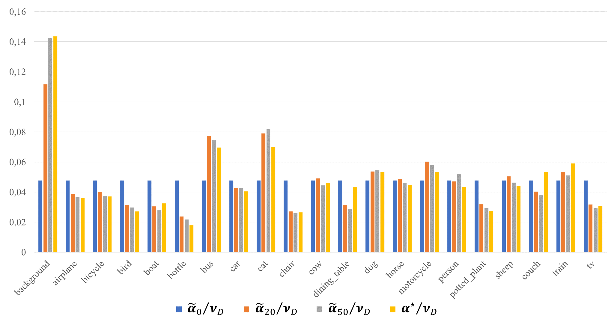
Given the above statements, it is natural to ask whether the normalised area converges to the ground truth normalised area , where is the ground truth area of category . We show experimentally that .
Figure 10 shows the evolution during training of the estimated average area distribution of categories for the PascalVOC2012[20] trainaug dataset [22], using for EMA update (see Eq. 7 in the main paper). Namely, we use Jensen–Shannon divergence () to assess the similarity between distributions. The red line in Figure 10 shows the divergence at epoch between and the ground truth area distribution of categories . This show, experimentally, that , for . The blue line in Figure 10 shows the convergence of the slow-moving distribution to a fixed target; that is, we compute the divergence at epoch between and to assess the magnitude of change of the distribution during the epochs. A similar graph can be shown between and .
In particular, as stated in Eq. 5 in the main paper, , which is used in Algorithm B, is defined to be , with the relative frequency of categories in the batch, here equal to 1 to obtain the unitary area. Noticing that is a constant, it follows that the above results also hold for . Therefore, in Figure 11 we show that the above-assessed similarity is consistently extended to up to a multiplicative factor proportional to , for all .
Appendix B Algorithmic Details
We present our pseudocode in Algorithm B. As stated in the main paper, we solve an optimal transport problem with regularised entropy penalty term to hasten convergence, which can be solved using a simple, alternate minimisation scheme. Since the objective is an -strongly convex function, problem in Eq. 3 has a unique optimal solution [41]. To do so we instantiate the Sinkhorn-Knopp algorithm following considerations in [41] and implementation in [15]. The number of iterations controls the trade-off between the optimality of the transport plan and computational cost. We empirically obtain the best compromise in terms of speed and performance, limiting the kernel balancing to 3 updates. A key insight is that, as , the optimal coupling becomes less and less sparse, and the solution leads to the tensor product . In contrast, as , the unique solution converges to the maximum entropy solution of the standard OT problem, and the convergence of Sinkhorn’s algorithm deteriorates [41]. We empirically found that using works the best in our experiments when using three iterations only. Moreover, we increase the value of with an exponential growth of rate for 40 epochs until reaching the final value of .
![[Uncaptioned image]](/html/2303.17410/assets/x3.png)
Appendix C Computational Cost
In this section, we analyse our framework’s computational cost in terms of space and time complexity. As highlighted in [44] ViT-based architectures have a memory footprint comparable with other weakly supervised segmentation models, as evidenced by the number of parameters of the model, which reaches 89.4 M. Regarding the running time of the model, we refer to Section 4.2 in the main paper. In Table 8, we show that the memory footprint of our unsupervised method is on par with other self-supervised frameworks.
| Model | Architectures | # Params () | mIoU% |
|---|---|---|---|
| Ours | ViT-B/16 + | ||
| ViT-PCM [44] (ViT-B/16) | 175 | 43.6 | |
| SemSpectral [35] | ViT-B/8 | ||
| DeepLab v3 (RN50) [7] (RN50) | 128 | 30.8 | |
| MaskContrast [52] | DeepLab v3 (DRN50) + | ||
| BASNet [43]+ | |||
| DeepUSPS [36] (DRN105) | 182 | 35.0 | |
| TransFGU [65] | 2*ViT-S/8 | ||
| + 2*Segmenter [49] (ViT-S/8) | 88 | 37.15 | |
| Leopart [69] | 2*ViT-B/8 | 172 | 41.7 |
Consider the optimisation problem in (3) with and let . For a large enough batch size, corresponds to the number of input patches. Finding solutions to the OT problem, computed via the Sinkhorn-Knopp (SK) algorithm, at each training iteration adds some computational cost to the proposed method. The time complexity of the SK algorithm is an active field of research; classical algorithms, such as the [37, 13], find solutions to the unregularised OT problem in . [15] showed that approximate solutions to the true minimum , such that , can be found relatively fast by solving the corresponding entropic regularised problem in (3). In particular, [2] provided an upper bound for the number of the arithmetic operations needed for convergence of the entropy-regularised SK algorithm: . Although without theoretical guarantees about the time complexity bound, [2] also provided a version of the SK algorithm, named GreenKhorn, which empirically performs better than the implementation by [15]. [19] recently improved on the results in [2] providing an algorithm with time complexity of . In our method, we use the SK implementation by [15], inducing a worst-case-scenario cost of for a dateset of dimension , at each epoch.
Appendix D Per-class accuracy in PascalVOC2012 and MS-COCO2014
This section presents additional tables for our results on the PascalVOC2012 dataset and the MS-COCO2014 datasets. In Table 9, we present the accuracy for the weakly-supervised segmentation task on MS-COCO2014 val set for each class and compare our results with the methods which have the best accuracy so far, namely MCTFormer [64] and ViT-PCM [44]. ViT-PCM already had the total best accuracy w.r.t. MCTFormer of 3 points in mIoU%, and we outperform ViT-PCM by about 1 point. In Table 10, we present the per-class mIoU% accuracy of our PC2M on the unsupervised segmentation task on MS-COCO2014 val set. Here we do not have available other methods to compare with. We can observe that for some classes such as ’baseball-bat’, ’fork’, ’spoon’ and ’toaster’, the mIoU accuracy is zero.
Table 11 reports the mIoU% accuracy for the two weakly-supervised and unsupervised semantic segmentation tasks on PascalVOC2012 val set. We observe that there is no proportion between the two methods. In the unsupervised task, some classes like ’boat’ are missed, and others classes like ’TV’, ’aeroplane and ’bus’ have an accuracy close to the one in the weakly-supervised task. Moreover, a common practice in WSSS is to test the accuracy of the generated pseudo-segmentations by using them as masks to train a standard segmentation model and compare the latter with the ground-truth supervised version. Interestingly, using our pseudo-masks to train DeepLabV3 [8] leads to a less accurate model than our PC2M, respectively 74.2% vs 75% mIoU. Nevertheless, both results are still competitive for the supervised DeepLabV3-JFT, which obtain 82.7% mIoU on PascalVOC2012 val set. See Table 11.
| Class | Ours (PC2M) | MCT-FormerCVPR’22 | ViT-PCMECCV’22 | Class | Ours (PC2M) | MCT-FormerCVPR’22 | ViT-PCMECCV’22 | ||
|---|---|---|---|---|---|---|---|---|---|
| [64] | [44] | [64] | [44] | ||||||
| 0. | background | 84.5 | 82.4 | 81.9 | 41. | wine-glass | 40.7 | 27.0 | 38.2 |
| 1. | person | 59.5 | 62.6 | 62.4 | 42. | cup | 37.5 | 29. | 40.9 |
| 2. | bicycle | 50.7 | 47.4 | 54.3 | 43. | fork | 8.1 | 13.9 | 33.3 |
| 3. | car | 48.7 | 47.2 | 49.2 | 44. | knife | 20.4 | 12.0 | 31.0 |
| 4. | motorcycle | 68.3 | 63.7 | 70.3 | 45. | spoon | 8.7 | 6.6 | 21.4 |
| 5. | airplane | 70.1 | 64.7 | 74.5 | 46. | bowl | 42.8 | 22.4 | 36.2 |
| 6. | bus | 70.9 | 78.6 | 76.0 | 47. | banana | 65.3 | 63.2 | 58.6 |
| 7. | train | 58.9 | 64.5 | 61.2 | 48. | apple | 54.1 | 44.4 | 52.1 |
| 8. | truck | 48.5 | 44.8 | 45.3 | 49. | sandwich | 39.4 | 39.7 | 57.1 |
| 9. | boat | 35.0 | 42.3 | 47.8 | 50. | orange | 65.9 | 63.0 | 55.8 |
| 10. | traffic-light | 46.2 | 49.9 | 22.2 | 51. | broccoli | 30.5 | 51.2 | 53.5 |
| 11. | fire-hydrant | 77.7 | 73.2 | 78.8 | 52. | carrot | 28.9 | 40.0 | 45.0 |
| 12. | stop-sign | 78.5 | 76.6 | 11.0 | 53. | hot-dog | 65.5 | 53.0 | 41.4 |
| 13. | parking-meter | 71.8 | 64.4 | 65.5 | 54. | pizza | 79.3 | 62.2 | 77.6 |
| 14. | bench | 40.9 | 32.8 | 42.6 | 55. | donut | 75.2 | 55.7 | 39.4 |
| 15. | bird | 69.0 | 62.6 | 67.0 | 56. | cake | 34.6 | 47.9 | 63.0 |
| 16. | cat | 82.2 | 78.2 | 20.4 | 57. | chair | 24.6 | 22.8 | 35.6 |
| 17. | dog | 77.2 | 68.2 | 71.7 | 58. | couch | 41.5 | 35.0 | 41.7 |
| 18. | horse | 69.2 | 65.8 | 68.6 | 59. | potted-plant | 26.0 | 13.5 | 37.9 |
| 19. | sheep | 77.0 | 70.1 | 67.2 | 60. | bed | 53.5 | 48.6 | 53.2 |
| 20. | cow | 76.4 | 68.3 | 70.4 | 61. | dining-table | 15.4 | 12.9 | 29.4 |
| 21. | elephant | 83.1 | 81.6 | 83.3 | 62. | toilet | 61.0 | 63.1 | 67.3 |
| 22. | bear | 85.0 | 80.1 | 74.2 | 63. | tv | 48.0 | 47.9 | 38.7 |
| 23. | zebra | 81.1 | 83.0 | 72.6 | 64. | laptop | 58.0 | 49.5 | 51.7 |
| 24. | giraffe | 76.0 | 76.9 | 67.3 | 65. | mouse | 14.3 | 13.4 | 13.9 |
| 25. | backpack | 18.4 | 14.6 | 24.3 | 66. | remote | 41.2 | 41.9 | 34.2 |
| 26. | umbrella | 69.0 | 61.7 | 67.7 | 67. | keyboard | 60.4 | 49.8 | 65.0 |
| 27. | handbag | 7.2 | 4.5 | 19.4 | 68. | cellphone | 60.5 | 54.1 | 56.8 |
| 28. | tie | 21.3 | 25.2 | 19.0 | 69. | microwave | 28.0 | 38.0 | 50.2 |
| 29. | suitcase | 52.5 | 46.8 | 47.6 | 70. | oven | 20.0 | 29.9 | 35.8 |
| 30 | . frisbee | 24.0 | 43.8 | 38.1 | 71. | toaster | 4.6 | 0.0 | 13.8 |
| 31. | skis | 3.1 | 12.8 | 20.3 | 72. | sink | 30.4 | 28.0 | 14.3 |
| 32. | snowboard | 17.5 | 31.4 | 41.6 | 73. | refrigerator | 11.0 | 40.1 | 44.9 |
| 33. | sports-ball | 8.0 | 9.2 | 7.1 | 74. | book | 38.1 | 32.2 | 40.6 |
| 34 | kite | 60.2 | 26.3 | 41.5 | 75. | clock | 56.4 | 43.2 | 51.3 |
| 35. | baseball-bat | 2.7 | 0.9 | 2.3 | 76. | vase | 24.7 | 22.6 | 25.0 |
| 36. | baseball-glove | 3.8 | 0.7 | 5.0 | 77. | scissors | 50.0 | 32.9 | 48.1 |
| 37 | skateboard | 19.9 | 7.8 | 10.3 | 78. | teddy-bear | 67.9 | 61.9 | 53.9 |
| 38 | surfboard | 34.9 | 46.5 | 45.9 | 79. | hair-drier | 20.9 | 0.0 | 13.4 |
| 39. | tennis-racket | 12.4 | 1.4 | 16.1 | 80. | toothbrush | 35.0 | 12.2 | 33.1 |
| 40. | bottle | 39.0 | 31.1 | 41.5 | mean | 45.92 | 42.0 | 45.0 |
| Classes | background | person | bicycle | car | motorcycle | airplane | bus | train | track | boat | traffic light |
|---|---|---|---|---|---|---|---|---|---|---|---|
| Accuracy | 69.0 | 4.4 | 35.8 | 1.1 | 55.4 | 32.8 | 51.2 | 23.1 | 25.1 | 17.5 | 39.6 |
| Classes | fire-hydrant | stop-sign | parking-meter | bench | bird | cat | dog | horse | ship | cow | elephant |
| Accuracy | 52.7 | 38.8 | 0.0 | 25.4 | 23.7 | 36.6 | 24.8 | 52.1 | 36.5 | 51.9 | 73.9 |
| Classes | bear | zebra | giraffe | backpack | umbrella | handbag | tie | suitcase | frisbee | skis | snowboard |
| Accuracy | 3.3 | 80.6 | 76.1 | 0.9 | 50.8 | 1.1 | 11.1 | 1.1 | 1.1 | 0.7 | 3.8 |
| Classes | sports-ball | kite | baseball-bat | baseball-glove | skateboard | surfboard | tennis-racket | bottle | wine-glass | cup | fork |
| Accuracy | 0.0 | 3.6 | 0.1 | 0.7 | 8.4 | 1.6 | 2.9 | 3.4 | 0.0 | 0.0 | 0.0 |
| Classes | knife | spoon | ball | banana | apple | sandwich | orange | broccoli | carrot | hot-dog | pizza |
| Accuracy | 0.0 | 0.0 | 14.5 | 58.8 | 0.0 | 36.4 | 24.0 | 16.1 | 0.0 | 0.3 | 66.1 |
| Classes | donut | cake | chair | coach | potted-plant | bed | dining-table | toilet | tv | laptop | mouse |
| Accuracy | 23.7 | 11.1 | 0.3 | 9.2 | 0.1 | 10.0 | 2.1 | 56.8 | 15.4 | 25.2 | 0.0 |
| Classes | remote | keyboard | cell | microwave | oven | toaster | sink | refrigerator | book | clock | vase |
| Accuracy | 0.1 | 0.0 | 17.8 | 14.6 | 4.5 | 0.0 | 12.8 | 0.1 | 7.8 | 49.1 | 22.4 |
| Classes | scissors | teddy-bear | hair-dryer | tooth-brush | mean | ||||||
| Accuracy | 6.2 | 56.7 | 0.0 | 0.3 | 19.5 |
| Task | bkg | aero | bike | bird | boat | btl | bus | car | cat | chair | cow | table | dog | horse | mbk | person | plant | sheep | sofa | train | tv | mean |
|---|---|---|---|---|---|---|---|---|---|---|---|---|---|---|---|---|---|---|---|---|---|---|
| WSSS | 92.8 | 87.4 | 49.0 | 90.7 | 73.9 | 77.2 | 87.4 | 82.0 | 87.3 | 40.7 | 86.5 | 33.3 | 89.2 | 88.7 | 82.5 | 77.2 | 66.6 | 91.7 | 49.4 | 78.5 | 62.5 | 75.0 |
| WSSS+DeepLabV3[8] | 92.7 | 86.8 | 45.8 | 82.6 | 70.7 | 75.4 | 92.4 | 83.8 | 90.7 | 42.2 | 86.2 | 41.2 | 89.2 | 86.2 | 78.7 | 77.4 | 57.1 | 84.7 | 45.0 | 82.0 | 66.5 | 74.2 |
| USS | 86.6 | 73.1 | 41.5 | 79.1 | 0.0 | 40.3 | 70.0 | 66.8 | 69.3 | 19.6 | 0.06 | 17.1 | 40.2 | 58.7 | 63.1 | 17.8 | 0.03 | 43.9 | 0.0 | 42.7 | 50.6 | 43.6 |
Appendix E Qualitative results and qualitative comparisons with other methods
This section compares our results with other weakly-supervised and unsupervised semantic segmentation methods on PascalVOC2012 val set and on MS-COCO2014 val set and shows our qualitative results.
E.1 Qualitative comparisons on PascalVOC2012
Weakly-supervised task. To assess our qualitative results, we compare the pseudo-masks obtained with our method with ViT-PCM [44] and MCTFormer [64]. ViT-PCM and MCTFormer currently get the best accuracy on weakly supervised segmentation. Results are illustrated in Figure 12 and Figure 13. Concerning MCTFormer [64], note that we have taken the images to make the comparison from the paper [64]; therefore, we have not chosen our best results. Still, in several images, it is clear that our method obtains more refined pseudo-masks than MCTFormer.
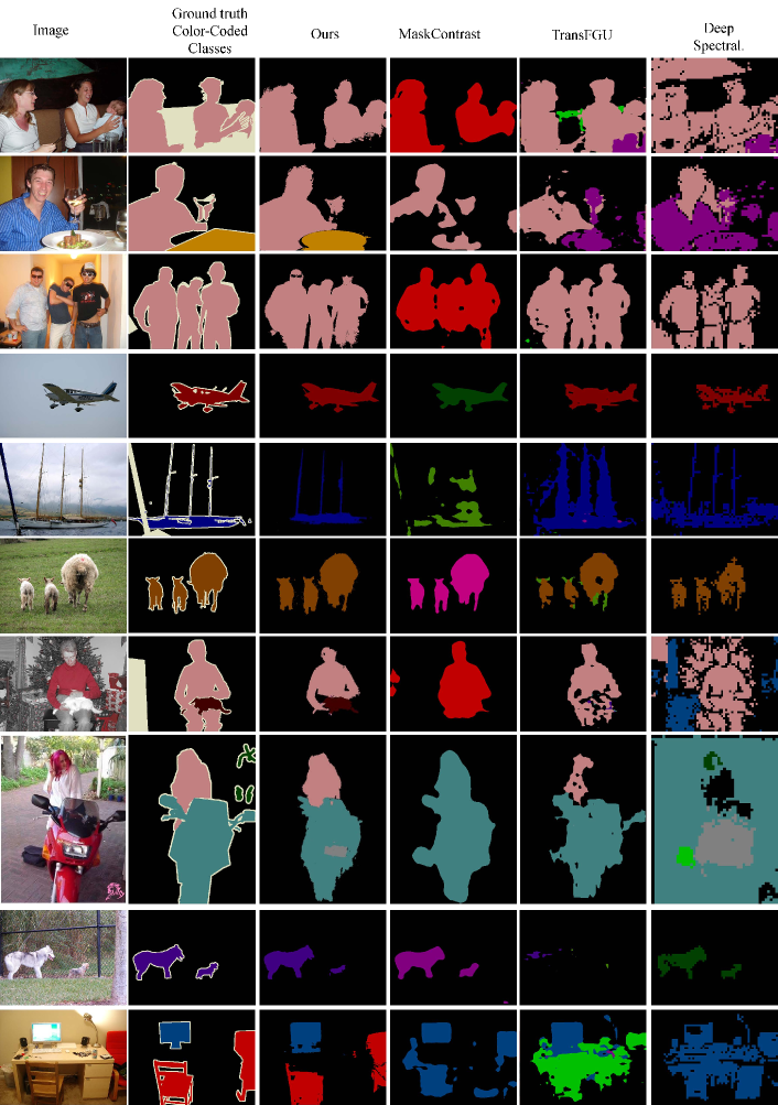
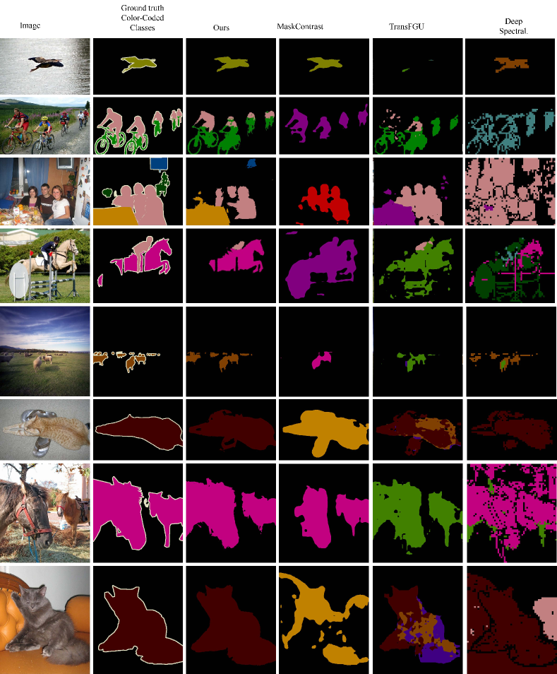
Unsupervised task. Here, we compare our results with three other approaches to unsupervised semantic segmentation. To produce the pseudo-mask and pseudo-labels, we have operated the publicly available software of MaskContrast [53], TransFGU[65], and Deep Spectral Segmentation [35]. First of all, we have verified that the declared results for each competitor were satisfied. In particular, for both MaskContrast and Deep Spectral Segmentation [35], we have used the PascalVOC2012 class colour palette to make it comparable with the other methods. The mapping to the PascalVOC2012 category set is obtained via the Hungarian algorithm to maximize the total mIoU%. Among our images returning correct classes, we have chosen those for which at least one of our competitors’ methods had a good shape or correct classes. See Figures 14 and 15. Figure 16 shows unsupervised masks on PascalVOC2012 val set.
E.2 Qualitative results on MS-COCO2014 val set
In Figure 18, we show our best mIoU% accuracy results for the WSSS task, while in Figure 17 we report our results on the USS task, on MS-COCO2014 val set. Finally, in Figure 19 we show qualitative comparisons of our weakly-supervised and unsupervised semantic segmentation results on MS-COCO2014 val. We intentionally show results in which segmentation masks are coherent for both methods, but objects are sometimes misclassified in the unsupervised setting, pointing to possible improvements in the image label clustering phase. Indeed, we observe low values for the generated pseudo multi-labels accuracy w.r.t. the ground-truth multi-labels, namely 42% macro F1-score and 37% micro F1-score on the MS-COCO2014 train set. Similarly, on the PascalVOC2012 trainaug set, we observe 53% macro F1-score and 51% micro F1-score.
Appendix F Considerations on the USS metrics
Currently used metrics for USS mix-up labels with shape accuracy. We would like to measure the shape accuracy for unsupervised semantic segmentation independently from the multi-label one. For each image , we consider the ground truth masks and the network predicted masks dropping the relative class ids. Thus we consider two sets of binary masks of cardinality . We use as the cost weight of the edges of a bipartite graph:
| (15) |
We solve the max cost associated with the graph, which does not imply the max match of the vertices. We take the average of all costs for each image in the validation set, obtaining . This metric clearly does not account for the semantics given by the multi-labels, but it singles out the geometric content of the image, which is a crucial aspect of USS. For our method, the over all images is 65.9% on PascalVOC2012 and 38.2% on MS-COCO2014 val sets.