Matrix Product Belief Propagation for reweighted stochastic dynamics over graphs

Abstract

Stochastic processes on graphs can describe a great variety of phenomena ranging from neural activity to epidemic spreading. While many existing methods can accurately describe typical realizations of such processes, computing properties of extremely rare events is a hard task. Particularly so in the case of recurrent models, in which variables may return to a previously visited state. Here, we build on the matrix product cavity method, extending it fundamentally in two directions: first, we show how it can be applied to Markov processes biased by arbitrary reweighting factors that concentrate most of the probability mass on rare events. Second, we introduce an efficient scheme to reduce the computational cost of a single node update from exponential to polynomial in the node degree. Two applications are considered: inference of infection probabilities from sparse observations within the SIRS epidemic model, and the computation of both typical observables and large deviations of several kinetic Ising models.

The problem of computing observables and marginal probabilities on a complex Markov process on large networks has been addressed extensively in the literature. While Monte-Carlo procedures can be often effective to compute averages approximately, they suffer from two separate issues: large relative sampling errors when computing averages that cancel out at the first order and they are limited to sampling “typical” events, as nontypical ones require an exponential number of samples. To address the first issue, many analytical solutions, mainly based on mean-field methods, have been devised [1, 2, 3, 4, 5, 6, 7]. A solution that is exact on acyclic graphs is Dynamic Cavity (DC) [8]. DC on general processes suffers from one main drawback, the fact that one must be able to represent the joint distribution of a single variable trajectory and a feedback field, and with some exceptions, the space of these trajectories is exponentially large (in the time horizon), and thus the approach becomes impracticable. One of these exceptions is on “non-recurrent” models, i.e. models in which each variable can only progress sequentially through a finite set of $k$ states, never going back to a previous state. In these cases the set of trajectories is polynomial in the time horizon (as an example with $q=3$, a trajectory $\left(1,1,2,2,2,2,3,3\right)$ on epochs $t=0,\dots,7$ can be represented by the integer tuple $\left(2,6\right)$ of epochs on which the variable effectively progresses to the next state in the sequence). Examples of non-recurrent models are the SI, SIR, SEIR compartmental models in computational epidemics, in which an individual can only transition from Susceptible to Exposed, from Exposed to Infective and from Infective to Recovered. While the use of non-recurrent models is pervasive, oftentimes a more realistic description demands that re-infections be taken into account. In such cases, “recurrent” models such as the SIS and SIRS are employed. Additionally, important processes in statistical physics such as Glauber dynamics belong to the class of models with recurrence.

In a recent work [9, 10], an interesting DC variant was proposed that exploits the Matrix Product State representation (MPS) to parametrize site trajectories and applied it to the Glauber dynamics on a Random Regular (RR) graph with degree 3. While these results are promising, the scheme suffers from two major limitations: first, it is computationally expensive (the update on a node of degree $z$ is of the order of $M^{2z-1}$ [10] where $M$ is the matrix dimension), making it impractical even for moderately large Erdos-Renyi (ER) random graphs, in which some large-degree vertices are surely present. Second, the scheme is devised to analyze a “free” dynamics without any sort of reweighting, which as we will see is necessary to study atypical trajectories. Matrix Product States, also known as Tensor Trains, are not new in physics and other areas of science, as they have been successfully applied both in many-body quantum systems [11, 12, 13], out-of-equilibrium statistical physics [14, 15], machine learning [16, 17] and more.

We propose an alternative approach, dubbed Matrix Product Belief Propagation (MPBP), based on the Pair Trajectory Belief Propagation formulation which was first introduced in [18]. It is closely related to DC but allows naturally to include non-negative reweighting terms on stochastic trajectories, thus allowing to study large deviations of the system. In practical terms, MPBP consist on a fixed point equation that is solved by iteration, whereas DC is solved sequentially in time, with a number of steps which is equal to the number of epochs of the dynamics. The latter approach is inherently limited to free dynamics: building trajectories sequentially in time makes it impossible to account for the effect of reweighting terms relative to future epochs.

The Julia code used to implement the method and produce the data presented in this work is publicly accessible at [19].

We describe in the following the models under consideration. Given a graph $G=\left(V,E\right)$ with $V=\left\{1,\dots,N\right\}$, consider a joint distribution over a set of discrete variables $\boldsymbol{x}=\{x_{1},\ldots,x_{N}\}$ throughout $T$ successive epochs of the form

$$p(\overline{\boldsymbol{x}})=\frac{1}{Z}\prod_{t=0}^{T-1}\prod_{i=1}^{N}f_{i}^{t+1}\left(x_{i}^{t+1},\boldsymbol{x}_{\partial i}^{t},x_{i}^{t}\right).$$ (1)

We use bold letters to indicate multiple variable indices $\boldsymbol{x}_{A}\equiv\{x_{j}\}_{j\in A}$ and overbars for multiple times indices $\overline{x}\equiv\{x^{t}\}_{t=0:T}$. Moreover, we indicate by $\partial i=\left\{j:\left(ij\right)\in E\right\}$ the set of neighbors of index $i$.

The form (1) includes (but notably is more general than) reweighted Markov dynamics $f_{i}^{t+1}(x_{i}^{t+1},\boldsymbol{x}_{\partial i}^{t},x_{i}^{t})=w(x_{i}^{0})^{\delta(t,0)}w(x_{i}^{t+1}|\boldsymbol{x}_{\partial i}^{t},x_{i}^{t})\phi_{i}^{t+1}(x_{i}^{t+1})$ with stochastic transitions $w$ and reweighting factors $\phi$

$$p(\overline{\boldsymbol{x}})=\frac{1}{Z}\prod_{i=1}^{N}w(x_{i}^{0})\prod_{t=0}^{T-1}w(x_{i}^{t+1}|\boldsymbol{x}_{\partial i}^{t},x_{i}^{t})\phi_{i}^{t+1}(x_{i}^{t+1}).$$ (2)

$\delta(y,z)$ is the Kroenecker delta which evaluates to $1$ if $y=z$, to $0$ otherwise, and $w(x_{i}^{0})$ is the initial state probability, which we take to be factorized over the sites.

Note that $Z=1$ in the absence of reweighting factors. Two types of reweighted dynamics of the form (2) will be used as running examples throughout this work. The first is Bayesian inference on a process of epidemic spreading. The posterior probability of the epidemic trajectory $\overline{\boldsymbol{x}}$ given some independent observations $\{O_{i}^{t}\}$ on the system is given by

$$p(\overline{\boldsymbol{x}}|O) =\frac{1}{p(O)}p(\overline{\boldsymbol{x}})p(O|\overline{\boldsymbol{x}}).$$ (3)

(3) can be seen as a particular case of (2), where $p(\overline{\boldsymbol{x}})=\prod_{i=1}^{N}w(x_{i}^{0})\prod_{t=0}^{T-1}w(x_{i}^{t+1}|\boldsymbol{x}_{\partial i}^{t},x_{i}^{t})$ and corresponds to the distribution of the free dynamics of the chosen epidemiological model, $p(O|\overline{\boldsymbol{x}})=\prod_{i}\prod_{t}p(O_{i}^{t}|x_{i}^{t})=\prod_{i}\prod_{t}\phi_{i}^{t}(x_{i}^{t})$ and $Z=p(O)$.

The simplest among the recurrent epidemiological models is the Susceptible-Infectious-Susceptible (SIS), where each individual starts with a probability $\gamma_{i}$ of being infectious at time zero. Then at each time step a susceptible node $i$ can be infected by each of its infectious neighbors $j\in\partial i$ with probability $\lambda_{ji}$, and an infectious node can recover with probability $\rho_{i}$. Observation terms $p(O_{i}^{t}|x_{i}^{t})$ are naturally used to model medical tests: $O_{i}^{t}$ is the outcome of a test performed on individual $i$ at time $t$. This formalism allows to incorporate information about the degree of accuracy of tests.

The second example is parallel Glauber dynamics for an Ising model at inverse temperature $\beta$ with couplings $\{J_{ij}\}$ and external fields $\{h_{i}\}$. Besides being one of the paradigmatic models in theoretical non-equilibrium statistical physics, Glauber dynamics is employed in the study of neural activity [20, 21]. It is defined by transitions

$$\tilde{w}(\sigma_{i}^{t+1}|\boldsymbol{\sigma}_{\partial i}^{t})=\frac{e^{\beta\sigma_{i}^{t+1}\left(\sum_{j\in\partial i}J_{ij}\sigma_{j}^{t}+h_{i}\right)}}{2\cosh\left[\beta\left(\sum_{j\in\partial i}J_{ij}\sigma_{j}^{t}+h_{i}\right)\right]}.$$ (4)

The dynamics does not converge to the equilibrium of the underlying Ising model $p_{J,h}(\boldsymbol{\sigma})=Z^{-1}\exp[-H_{J,h}(\boldsymbol{\sigma})]$, but it allows to compute observables of interest in some cases (see the Supplementary Information).

Moreover, we will allow $\sigma_{i}$ to stay in the same state with probability $p_{0}$. The transition thus becomes

$$w(\sigma_{i}^{t+1}|\boldsymbol{\sigma}_{\partial i}^{t},\sigma_{i}^{t})= (1-p_{0})\tilde{w}(\sigma_{i}^{t+1}|\boldsymbol{\sigma}_{\partial i}^{t})+$$

$$+p_{0}\delta(\sigma_{i}^{t+1},\sigma_{i}^{t}).$$ (5)

In the limit $p_{0}\to 0$, the stationary distribution converges to $p_{J,h}$ because the dynamics reduces to an asynchronous one (two or more simultaneous state changes happen with probability $\mathcal{O}(p_{0}^{2})$). See also the Supplementary Information.

Additionally, such dynamics can be “tilted” with e.g. a term $\prod_{i}\phi_{i}^{T}(\sigma_{i}^{T})=\prod_{i}e^{h\sigma_{i}^{T}}$ in order to study atypical trajectories. Note that other models studied in physics such as Bootstrap Percolation can be remapped into Glauber dynamics [22].

Related work

Mean-field methods

We briefly review the main features of existing approaches based on the cavity method. Dynamic Message Passing (DMP) [2, 23, 24] and the Cavity Master Equation [7, 6] are simple and fast approximate methods that were originally formulated on continuous time as ODEs for a vector of single-edge quantities (such as cavity magnetizations). Both methods are exact on acyclic graphs on non-recurrent models (such as SI or SIR), but only approximate on non-non-recurrent ones, and do not allow for atypical trajectories. $n$-step Dynamic Message Passing [3] makes an $n$-Markov ansatz on messages, exploring mainly $n=1$; its features are essentially those of DMP, with the difference that it applies to discrete time evolution and describes explicitly interactions at distance $n$ in time. Different flavors of the cluster variational method [5, 25] approximate the dynamics by treating exactly correlations between variables that are close either in time or space. Large deviations have been studied in [26] using a perturbation theory in the particular case of Glauber dynamics on a chain. Table 1 summarizes the features of the methods mentioned above. We take into consideration: ability to deal with reweighted dynamics, to deal with recurrent models, and to compute autocorrelations at arbitrary (time) distance.

	reweighting	Recurrent models	Autocorrelations
BP for non-recurrent models [18]	Y	N	Y
IBMF [1], DMP [2, 24, 3], CME [6]	N	Y	N
Dynamic Cluster Variational [5]	*	Y	Only two-times
Matrix Product Dynamic Cavity [9]	N	Y	Y
Matrix Product Belief Propagation	Y	Y	Y

Table 1: Features of existing analytical methods for the description of stochastic dynamics on graphs, Y for yes, N for no. The asterisks mean that the method could in principle be extended to include the considered feature although this has not, to the best of our knowledge, been done in the literature. IBMF stands for Individual-Based Mean Field, DMP for Dynamic Message Passing, CME for Cavity Master Equation. We did not include the perturbative approach [26] because it focuses on a very particular setting.

Monte Carlo

Throughout this work, the performance of algorithms is compared with Monte Carlo simulations. To estimate observables in a reweighted dynamics of the form (2) we employ a weighted sampling technique (see e.g. [27]): the posterior average of an observable $f$ is approximated by

$$\hat{f}=\frac{\sum_{\mu=1}^{M}\prod_{i,t}\phi_{i}^{t}\left((x_{i}^{t})^{(\mu)}\right)f\left(\boldsymbol{\overline{x}}^{(\mu)}\right)}{\sum_{\mu=1}^{M}\prod_{i,t}\phi_{i}^{t}\left((x_{i}^{t})^{(\mu)}\right)}$$ (6)

where $\left\{\boldsymbol{\overline{x}}^{(\mu)}\right\}_{\mu}$ are $M$ independent samples drawn from the prior $\prod_{i=1}^{N}w(x_{i}^{0})\prod_{t=0}^{T-1}w(x_{i}^{t+1}|\boldsymbol{x}_{\partial i}^{t},x_{i}^{t})$. Such strategy, however, turns out to be computationally prohibitive whenever the reweighting terms $\phi$ put most of the probability mass on atypical trajectories, which are (exponentially) unlikely to ever be sampled.

Matrix Product Belief Propagation

For the dynamic version of Belief Propagation (BP), we start with (1) as a distribution for single site trajectories $\overline{x}_{i}$. The associated factor graph would present many small loops due to the presence of both $\overline{x}_{i}$ and $\overline{x}_{j}$ in factors $f_{i}$ and $f_{j}$. Therefore, we work directly on the so-called dual factor graph where variables are pair of trajectories $(\overline{x}_{i},\overline{x}_{j})$ living on the edges of the original graph. For more details about this step we refer the reader to [18, fig. 3, eqns 8,9]. The BP equations on the dual factor graph read

$$m_{i\to j}(\overline{x}_{i},\overline{x}_{j})\propto \sum_{\overline{x}_{\partial i\setminus j}}\prod_{t=0}^{T-1}f_{i}^{t+1}(x_{i}^{t+1},\boldsymbol{x}_{\partial i}^{t},x_{i}^{t})$$

$$\times\prod_{k\in\partial i\setminus j}m_{k\to i}(\overline{x}_{k},\overline{x}_{i}).$$ (7)

Since the number of joint trajectories $(\overline{x}_{i},\overline{x}_{j})$ is exponentially large in $T$, an exact representation of the messages is in general computationally unfeasible. Here, similarly to [9], we parametrize messages in terms of matrix product states [13, 12, 11], also known as tensor trains in the mathematical literature [28]. Following the jargon of tensor networks, in the rest of the paper we will refer to the size of the matrices as bond dimension. For a wide class of dynamics including Glauber with $J_{ij}=\pm J$ and epidemic spreading with homogeneous infectivity, the computational cost for a single BP iteration is $\mathcal{O}(T|E|M^{6})$ where $T$ is the number of epochs, $|E|$ is the number of edges in the graph and $M$ is the bond dimension. In all the applications we considered, small bond dimension (scaling at most polynomially with $T$) was enough to obtain almost exact results. The full description of the approach is found in the Methods section.

Results

In this section we illustrate the effectiveness of MPBP applied to dynamics of epidemic spreading and of the kinetic Ising model. We first focus on free dynamics, showing results that are at least comparable with the existing methods, often more accurate. Then we move to reweighted processes, where our approach really represents an innovation.

Risk assessment in Epidemics

As examples of free dynamics, we estimate the marginal probability of an individual being in the infectious state under the SIS model, in several settings (fig. 1).

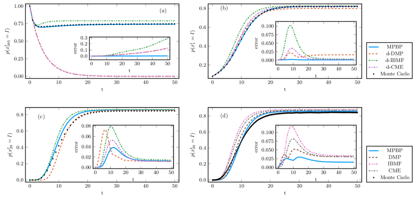
Figure 1: Marginal probabilities of free dynamics under the SIS model, comparison with models mentioned in the text. The main panels correspond to marginals for a single node of the graph, insets show the average absolute error over all nodes with respect to Monte Carlo simulations. Panels (a-c) compare against discretized versions of DMP, IBMF and CME (here with a "d-" prefix) and the Monte Carlo strategy reported in the text, panel (d) against regular continuous-time versions and a Gillespie-like Monte Carlo simulation. (a) Marginal of node $395$, the most connected one of a random tree with $N=1000$ nodes, $\lambda=0.3,\rho=0.2$. Node $395$ is the only infectious at time zero. Bond dimension $12$. (b) Marginal of node $1$ of a ER graph with $N=1000$ nodes, average connectivity $c=5$, $\lambda=0.1,\rho=0.05,\gamma=0.08$. Bond dimension $10$. (c) Marginal of node $29$ (zero-based numbering to match previous works) of Zachary’s karate club network, $N=34$ nodes, $\lambda=0.1,\rho=0.05$, node $0$ is the only infectious at time zero. Bond dimension $10$. (d) Same as (c) but the comparison is with continuous-time methods, with the addition of CME.

On a random tree and on a diluted random graph, both of size $N=1000$, MPBP shows almost no discrepancy with Monte Carlo averages (fig. 1a, 1b). In the former case a single node was picked as the sole infectious individual at time zero, in the latter a uniform probability $\gamma_{i}\equiv\gamma$ was put on each node. As a comparison we report the curves obtained using a discrete-time version of Dynamic message Passing (DMP) [24], Individual-Based Mean Field (IBMF) [1], and Cavity Master Equation (CME) [6], which were originally devised for continuous time evolution (more details in the supplementary information). We evaluate the accuracy of each method by considering the average absolute error with respect to a Monte Carlo simulation $\frac{1}{N}\sum_{i=1}^{N}\left|p(x_{i}^{t}=I)-p^{MC}(x_{i}^{t}=I)\right|$ (insets of fig. 1). The same analysis is repeated on Zachary’s karate club graph [29] (fig. 1c), the same benchmark used in [24, 7]. It must be pointed out that although MPBP shows by far the best performance in these comparison, the other considered methods are significantly simpler. None of the analytic methods is devised to analyze reweighted dynamics. Finally, we compare MPBP against three continuous-time methods, DMP, IBMF and CME, on the karate club graph (fig. 1d). The comparison is made by multiplying the transmission and recovery rates for the continuous setting $\lambda,\rho$ by the time-step $\Delta t$ (in this case $\Delta t=1$) to turn them into probabilities to be handled by MPBP. MPBP gives the best overall prediction across the considered window.

Moving to reweighted processes, fig. 2 shows the efficacy of MPBP when performing inference of trajectories given some observations. On a small ($N=23)$ random graph, a 10-step trajectory $\overline{\boldsymbol{y}}$ was sampled from a SIS prior distribution with $\lambda=0.15,\rho=0.12,\gamma=0.13$. We then observed the state of a random half $I\subset V$ of the nodes, added the corresponding reweighting factors $\prod_{i\in I}\phi_{i}^{T}(x_{i}^{T})=\prod_{i\in I}\delta(y_{i}^{T},x_{i}^{T})$ and performed inference using (3).

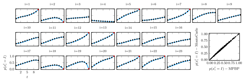
Figure 2: MPBP (solid line) with bond dimension $3$ correctly computes marginals of an SIS model defined on an Erdos-Renyi graph with $23$ nodes and average connectivity $4$, $\lambda=0.15,\rho=0.12,\gamma=0.13$. The state of a random half of the variables was observed at final time $T=10$ and used to reweight the distribution (red dots). Black dots are the average over $10^{6}$ Monte Carlo simulations. (Bottom-right) Comparison of all points from the previous plots, the Pearson correlation coefficient is $0.9986$.

The MPBP estimate for the posterior marginals, obtained with matrices of size $3$, agrees almost perfectly with Monte Carlo simulations. This is good indication that MPBP applied to sparse problems will keep giving accurate results even when on larger and/or more constrained instances where Monte Carlo methods fail, leaving little to compare against.

Realistic scenarios are often better described by the Susceptible-Infectious-Recovered-Susceptible (SIRS) model where transmission of infections is analogous to the SIS case, but an infectious node $i$ can recover with probability $\rho_{i}$ and a recovered become susceptible again with probability $\sigma_{i}$. From a practical point of view, extending the SIR to SIRS in the MPBP framework takes little effort: it suffices to enrich the factors with the new transition $R\to S$. Fig. 3 shows the performance of MPBP at estimating the posterior trajectories for a single realization of an epidemic drawn from a prior whose parameters $\lambda,\rho,\sigma,\gamma$ are homogeneous and known.

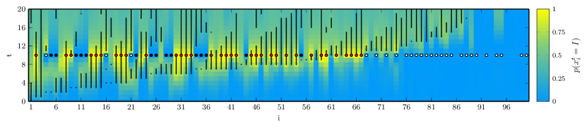
Figure 3: Inference on a single epidemic outbreak sampled from a SIRS model on an Erdos-Renyi graph with average connectivity $c=2.5$, $N=100$. Bond dimension $M=3$. The process to be inferred was drawn from a SIRS prior with $\lambda=0.4,\rho=\sigma=0.15,\gamma=0.01$, the same parameters were used for the inference. The state of $75\%$ of the nodes was observed at time $10$ (white=S, red=I, black=R) and used to reweight the distribution. Black lines correspond to true infection periods.

The state of a random $75\%$ of the system was observed at an intermediate time (colored dots). We see good agreement between the true infection times (black lines) and the marginal probabilities of being Infectious (in yellow). Nodes are sorted in increasing order of true first infection time.

Kinetic Ising

As examples of free dynamics we consider the evolution of magnetization $\langle\sigma_{i}^{t}\rangle$ and time autocovariance $\langle\sigma_{i}^{t}\sigma_{i}^{s}\rangle-\langle\sigma_{i}^{t}\rangle\langle\sigma_{i}^{s}\rangle$ for pairs of epochs $(t,s)$, on ferromagnetic, Random Field and spin-glass Ising Models (fig. 4), under the stochastic transition (5).

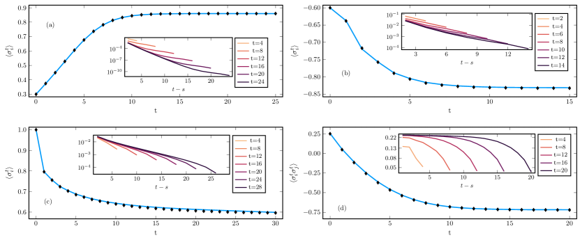
Figure 4: Magnetization $\langle\sigma_{i}^{t}\rangle$ (a-c) or nearest-neighbor correlation $\langle\sigma_{i}^{t}\sigma_{j}^{t}\rangle$ (d) as a function of time for different Ising models. Solid lines are MPBP, dots are Monte Carlo simulations on graphs of size $N_{MC}$, dashed horizontal lines are the equilibrium values (a-c) or 1RSB prediction (d) for the corresponding static versions of the models. Insets show autocovariances $\langle\sigma_{i}^{t}\sigma_{i}^{s}\rangle-\langle\sigma_{i}^{t}\rangle\langle\sigma_{i}^{s}\rangle$, only even epochs are shown for panels (a-c) because of odd-even effects in the dynamics of ferromagnetic models (as in [9, 25]). (a) Infinite $8$-Random Regular Graph, $\beta J=0.2$, $N_{MC}=5000$, bond dimension $25$. (b) Infinite Erdos-Renyi graph with mean connectivity $c=4$, $\beta J=0.5$, $N_{MC}=5000$, bond dimension $18$. (c) Random Field Ising Model on Erdos-Renyi graph with mean connectivity $c=3,\beta J=2/c$, $N=N_{MC}=1000$ and $\beta h_{i}=\pm 0.6$ sampled uniformly, matrix size $10$. (d) Antiferromagnetic Ising Model on infinite $3$-Random Regular Graph with $J=-1,\beta=\infty$, $N_{MC}=5000$, bond dimension $23$.

First we consider a model with uniform couplings $J_{ij}\equiv J$ on an infinite Random Regular Graph like the one studied in [9] but with degree $8$ instead of $3$. We then apply our method to an infinite Erdos-Renyi graph, again with uniform couplings and in the ferromagnetic phase, using a population dynamics approach. Next, we study a Random Field Ising Model (RFIM) with uniform couplings and random external fields $h_{i}=\pm h$ on a large graph. In all three cases the system is initialized in a magnetized state and the fraction of up spins grows or decreases monotonically until it reaches a stationary value. For these second and third models we picked the same settings as in [25]. Finally, we consider an antiferromagnetic model with $J=-1$ at zero temperature ($\beta=\infty$), focusing on the nearest-neighbor correlation $\langle\sigma_{i}^{t}\sigma_{j}^{t}\rangle$, $(i,j)\in E$ rather than the magnetization, which is null at steady state. Above the critical inverse temperature $\beta_{c}=\log\left(1+\sqrt{2}\right)$ [30], the underlying Ising system is in a glassy phase. For this model we used the modified version of the dynamics reported in (5) with $p_{0}=0.25$.

Finally, we study the large deviation behavior of a free dynamic $W(\overline{\boldsymbol{\sigma}})=\prod_{i=1}^{N}w(\sigma_{i}^{0})\prod_{t=0}^{T-1}w(\sigma_{i}^{t+1}|\boldsymbol{\sigma}_{\partial i}^{t})$ by tilting it with an external field at final time $\prod_{i}\phi_{i}^{T}(\sigma_{i}^{T})=\prod_{i}e^{h\sigma_{i}^{T}}$. In the thermodynamic limit $N\to\infty$ this allows to select a particular value for the magnetization at final time $m=\frac{1}{N}\sum_{i}\sigma_{i}^{T}$. The Bethe Free Energy computed via MPBP is an approximation for

$$f(h)= -\frac{1}{N}\log\sum_{\{\sigma_{i}^{t}\}_{i,t}}W(\overline{\boldsymbol{\sigma}})e^{h\sum_{i}\sigma_{i}^{T}}$$ (8)

$$= -\frac{1}{N}\log\sum_{m}e^{-N[g(m)-hm]}$$ (9)

$$\xrightarrow{N\to\infty} \min_{m}\left\{g(m)-hm\right\}$$ (10)

$$= g(m(h))-hm(h)$$ (11)

where $g(m)=-\frac{1}{N}\log\sum_{\{\sigma_{i}^{t}\}_{i,t}}W(\overline{\boldsymbol{\sigma}})\delta\left(Nm,\sum_{i}\sigma_{i}^{T}\right)$, and $m(h)=\arg\min_{m}\left\{g(m)-hm\right\}$. In regions where $g(m)$ is convex, the Legendre transform (10) can be inverted to obtain a large deviation law for the probability of observing the system at final time with magnetization $m$

$$p(m)\sim e^{-N\left[f\left(h(m)\right)+mh(m)\right]}$$ (12)

where $h(m)$ is the inverse of $m(h)$. Fig. 5 shows the estimate of $g(m)$ for a ferromagnetic Ising model on an infinite random graph initialized at magnetization $m^{0}=0.1$ and evolving for $T=10$ epochs. $p(m)$ has a minimum at $m\approx 0.145$ which corresponds to the free dynamics $h=0$.

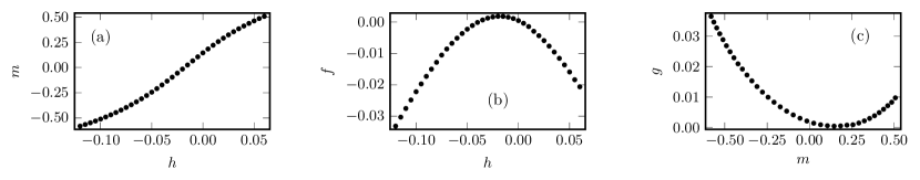
Figure 5: Large deviation study of Glauber dynamics on an infinite 3-Random Regular Graph. Free dynamics with $\beta J=0.6$, $T=10$, magnetization at time zero $m^{0}=0.1$, zero external field, reweighted with an external field at final time $\prod_{i}\phi_{i}^{T}(\sigma_{i}^{T})=\prod_{i}e^{h\sigma_{i}^{T}}$. (a) Magnetization vs reweighting field, (b) Bethe Free Energy vs reweighting field, (c) Magnetization-constrained free energy $g(m)$ vs magnetization. Bond dimension $25$.

Such an analysis could not have been carried out by means of Monte Carlo methods since the probability of sampling a trajectory ending at $m$ is infinitesimal, as is clear from the large deviation law in fig. 5.

Discussion

It is often the case that stochastic processes which can be described accurately, be it by analytical or Monte-Carlo methods, become computationally difficult as soon as the dynamics is biased by some reweighting factor. This constitutes a massive limitation since reweighting is essential whenever one is interested in describing atypical trajectories, an emblematic example being inference in epidemic models. As of today there exist, to the best of our knowledge, no analytic method able to describe reweighted complex dynamics on networks except for the simple case of non-recurrent models. In this article we adopted the matrix-product parametrization, inspired by techniques used originally in quantum physics and recently applied to classical stochastic dynamics in [9], to devise the Matrix Product Belief Propagation method. We used it to describe reweighted Markov dynamics on graphs, and applied it to epidemic spreading and a dynamical Ising models. With respect to the important work in [9, 10], which we recall that applies only to free dynamics, our contribution is twofold.

First, we develop for MPBP a general scheme to render the computation time linear in the node degree rather than exponential on a wide class of models, allowing us to compare it extremely favorably with existing methods on standard benchmark examples (which typically include vertices with large degrees). The bottleneck of the whole computation in the final scheme is due to the SVD factorization, which are cubic in the bond dimension $M$: larger matrices give a better approximation, but require a greater computational effort. The overall cost per iteration, assuming the bond dimension constant, is $O\left(T\left|E\right|\right)$, i.e. linear in the number of edges of the graph. A small number of iterations is normally sufficient for approximate convergence a fixed point. A strategy we found to be effective is to start with matrix size $M$ very small, say $4$ or $5$, iterate until convergence, then repeat with increasingly larger $M$. It is fair to point out, however, that although linear, depending on the target accuracy of the approximation defined by the parameter $M$, the method may be substantially more computationally intensive than the others used for comparison.

Second and more importantly, the MPBP approach allows to include reweighting factors. In particular, the approach proposed in [9, 10] is iterated forward in (dynamical) time, and thus allows no backward flow of information which is necessary with reweighting factors. Reweighting factors are necessary to analyze conditioned dynamics and rare events.

MPBP, like many other statistical physics-inspired approaches to stochastic dynamics, is based on the cavity approximation. The Belief Propagation formalism gives access to the thermodynamic limit for certain ensembles of random graphs, provides an approximation to the partition function through the Bethe Free Energy, and allows to compute time autocorrelations. The limits of validity of MPBP are inherited from those of the cavity approximation: using the jargon of disordered systems, the approximation is accurate as long as the problem is in a Replica Symmetric (RS) phase. In the case of epidemic inference presented in fig. 3 this is surely the case, since the trajectory to be inferred was sampled from the same prior used for the inference. This amounts to working on the Nishimori line, where it is known that no replica symmetry-breaking takes place [31]. A study of the performance in regimes where replica symmetry is broken is left for future investigation.

On graphs with short loops, the performance of BP degrades substantially. In the static case, this issue can sometimes be overcome by resorting to higher order approximations [32]. We argue that the same ideas can be translated to dynamics, for example by describing explicitly the joint trajectory of quadruples of neighboring variables on a square lattice.

Software implementing the method is available at [19] and can be used to directly reproduce the results in the article. The framework is flexible and accommodates for the inclusion of new models of dynamics.

As a final remark, we recall that the method applies more in general to any distribution of the type (1), where $t$ need not be interpreted as a time index but could, for instance, span a further spatial direction. Investigation along this line is left for future work.

Materials and methods

As anticipated, messages are parametrized in terms of matrix products

$$m_{i\to j}(\overline{x}_{i},\overline{x}_{j})\propto \prod_{t=0}^{T}A_{i\to j}^{t}(x_{i}^{t},x_{j}^{t})$$ (13)

where, for any $(x_{i}^{t},x_{j}^{t})$, $A_{i\to j}^{t}(x_{i}^{t},x_{j}^{t})$ is a real-valued matrix. We set $A^{0}$ to have one row and $A^{T}$ to have one column, so that the whole product gives a scalar. Plugging the ansatz (13) into the RHS of the BP equation (7) gives

$$m_{i\to j}(\overline{x}_{i},\overline{x}_{j})\propto\prod_{t=0}^{T}B_{i\to j}^{t}(x_{i}^{t+1},x_{i}^{t},x_{j}^{t})$$ (14)

with

$$B_{i\to j}^{t}(x_{i}^{t+1},x_{i}^{t},x_{j}^{t})= \sum_{\{x_{k}^{t}\}_{k\in\partial i\setminus j}}f_{i}^{t+1}(x_{i}^{t+1},\boldsymbol{x}_{\partial i}^{t},x_{i}^{t})$$

$$\times\left[\bigotimes_{k\in\partial i\setminus j}A_{k\to i}^{t}(x_{k}^{t},x_{i}^{t})\right].$$ (15)

Two steps are missing in order to close the BP equations under a matrix product ansatz, as discussed in [9]. First, matrices must be recast into the form (13). Second, if incoming $A$ matrices have bond dimension $M$, $B$ matrices will have bond dimension $M^{|\partial i|-1}$ and thus will keep growing indefinitely throughout the iterations. Both issues are solved by means of two successive sweeps of Singular Value Decompositions (SVD). SVD decomposes a real-valued matrix $A$ as $A_{ij}=\sum_{k,l=1}^{M}U_{ik}\Lambda_{kl}V_{jl}$ where $\Lambda_{kl}=\lambda_{k}\delta_{k,l}$ is the diagonal matrix of singular values $\lambda_{1}\geq\lambda_{2}\geq\ldots\geq\lambda_{M}\geq 0$ and $U^{\dagger}U=VV^{\dagger}=\mathds{1}$ (we use the dagger symbol for matrix transpose to avoid confusion with the time labels $t,T$, but all matrices are real-valued). By retaining only the largest $M^{\prime}$ singular values and setting the others to zero, one can approximate $A_{ij}$ with $\widetilde{A}_{ij}\coloneqq\sum_{k=1}^{M^{\prime}}U_{ik}\lambda_{k}V_{jk}$ making an error $\lVert A-\widetilde{A}\rVert_{F}^{2}=\sum_{ij}\left(A_{ij}-\widetilde{A}_{ij}\right)^{2}=\sum_{k=M^{\prime}+1}^{M}\lambda_{k}^{2}$. As a result, both $U$ and $V$ are smaller in size.

The first sweep is done from left to right $t=0,1,2,\ldots,T-1$ by performing an SVD decomposition

$$B_{i\to j}^{t}(x_{i}^{t+1},x_{i}^{t},x_{j}^{t})=C_{i\to j}^{t}(x_{i}^{t},x_{j}^{t})\Lambda^{t}\left[V^{t}(x_{i}^{t+1})\right]^{\dagger}$$ (16)

then redefine $B_{i\to j}^{t+1}(x_{i}^{t+2},x_{i}^{t+1},x_{j}^{t+1})$ as $\Lambda^{t}\left[V^{t}(x_{i}^{t+1})\right]^{\dagger}B_{i\to j}^{t+1}(x_{i}^{t+2},x_{i}^{t+1},x_{j}^{t+1})$. The decomposition in (16) is performed by incorporating $x_{i}^{t},x_{j}^{t}$ as row indices and $x_{i}^{t+1}$ as column index (see the supplementary information for more details). At the end of this first sweep, the message looks like

$$m_{i\to j}(\overline{x}_{i},\overline{x}_{j})=\prod_{t=0}^{T}C_{i\to j}^{t}(x_{i}^{t},x_{j}^{t})$$ (17)

where, thanks to the properties of the SVD, it holds that

$$\sum_{x_{i}^{t}x_{j}^{t}}\left[C_{i\to j}^{t}(x_{i}^{t},x_{j}^{t})\right]^{\dagger}C_{i\to j}^{t}(x_{i}^{t},x_{j}^{t})=\mathbb{\mathds{1}}.$$ (18)

At this point the form (13) is recovered: the BP equations are closed under a matrix product ansatz. All that is left to do is perform a second sweep of SVD, this time discarding the smallest singular values to obtain matrices of reduced size. Going right to left $t=T,T-1,\ldots,1$, incorporating $(x_{i}^{t},x_{j}^{t})$ as column indices:

$$C_{i\to j}^{t}(x_{i}^{t},x_{j}^{t}) \stackrel{{\scriptstyle{\rm SVD,trunc}}}{{\eqqcolon}}U^{t}\Lambda^{t}A_{i\to j}^{t}(x_{i}^{t},x_{j}^{t})$$ (19)

$$C_{i\to j}^{t-1}(x_{i}^{t-1},x_{j}^{t-1}) \leftarrow C_{i\to j}^{t-1}(x_{i}^{t-1},x_{j}^{t-1})U^{t}\Lambda^{t}$$

The errors made during the truncations are controlled: consider a generic step $t$ in the sweep from right to left. The MPS is in the so-called mixed-canonical form [33]:

$$C^{0}\cdots C^{t}A^{t+1}\cdots A^{T}$$ (20)

with $C^{0}\cdots C^{t-1}$ left-orthogonal ($C^{\dagger}C=\mathds{1}$) and $A^{t+1}\cdots A^{T}$ right-orthogonal ($AA^{\dagger}=\mathds{1}$). $C^{t}$ is neither.

Canonical forms are a useful tool to perform controlled truncations [28, 33]. The error in replacing $C^{t}$ by $\widetilde{C}^{t}$ which retains only $M^{\prime}$ of the $M$ singular values is

$$\lVert C^{0}\cdots C^{t}A^{t+1}\cdots A^{T}-C^{0}\cdots\widetilde{C}^{t}A^{t+1}\cdots A^{T}\rVert_{F}^{2}$$

$$=\lVert C^{t}-\widetilde{C}^{t}\rVert_{F}^{2}=\sum_{k=M^{\prime}+1}^{M}\lambda_{k}^{2}$$ (21)

where the first equality holds thanks to the orthonormality of $C$ and $A$ matrices. Keeping the MPS in canonical form ensures that the global error on the matrix product reduces to the local error on $C^{t}$.

As a side remark, we point out that there exist techniques to compute directly the SVD truncated to the $M^{\prime}$ largest singular values [34, 35]. Such strategies can be advantageous for large $M$ and small $M^{\prime}$.

The results in this work were obtained by fixing the number of retained singular values, and hence the bond dimension. Alternatively, given a target threshold $\varepsilon$, one can select $M^{\prime}$ adaptively such that, e.g. $\frac{\lambda_{M^{\prime}}}{\sqrt{\sum_{k}\lambda_{k}^{2}}}<\varepsilon$, as in [9]. We find the approach with fixed bond dimension better suited for an iterative solver such as BP, where messages are computed and then overwritten many times before convergence is reached. During the first iterations a coarse approximation with small bond dimension is sufficient and helps to keep the computation time under control. Then, as messages approach a fixed point, one can refine the estimate by either increasing the bond dimension or switching to a threshold-based truncation method.

Bond dimension

Issues may arise whenever excessive truncations turn the matrix product into an ill-defined probability distribution taking negative values. This is to be expected and indeed was encountered in the experiments we run. Re-running BP with larger bond dimension invariably solved the problem. Figure 6 shows the effect of varying the bond dimension in two of the settings shown in the previous plots. Instead, truncating too much may lead to unreasonable results such as negative probability values.

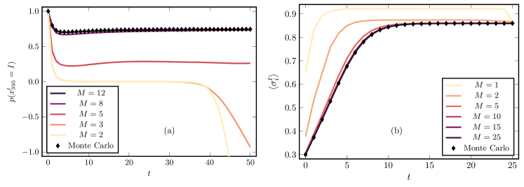
Figure 6: Effect of varying the bond dimension $M$ on the accuracy of the approximation. (a) SIS model on a tree, the same settings as figure 1a. Too small bond dimension gives unreasonable results. (b) Glauber dynamics on infinite random regular graph of degree $8$, same settings as figure 4a.

Turning to the expressive power of the MPS ansatz, it is reasonable to expect that truncating conservatively, i.e. allowing large bond dimension, will lead to better and better approximations. Indeed, matrix products with arbitrarily large bond dimension can represent exactly any distribution. However, it is hard to make quantitative statements about the relationship between bond dimension and the complexity that can be captured. Based on the discussion in the context of quantum mechanics (see e.g. [33, section 4.2.2]), it is plausible to assume that strong and long-range (here in time, in the quantum context these are usually in space) correlations need large matrices to be captured accurately. However this cannot possibly be the whole story, since there exists a simple counterexample: any trajectory of the SI epidemic model can be represented using MPS of finite bond dimension despite featuring infinite-range correlations. More details are found in the supplementary information.

Convergence

The BP equations are iterated until convergence to a fixed point. We opted for an asynchronous update scheme because it tends to feature better convergence properties with respect to a synchronous one. Nevertheless, the two can be used interchangeably. As usual with BP, the procedure naturally lends itself to parallelization, to a larger extent with the synchronous approach.

As a criterion for convergence to a fixed point we computed the marginal distributions at all nodes and epochs $b_{i}^{t}(x_{i}^{t})$ (see (23)) and checked whether, for an iteration $it$ and the successive one,

$$\max_{i\in\{1,\ldots,N\}}\max_{t\in\{0,\ldots,T\}}\max_{x_{i}^{t}}\left|\left[b_{i}^{t}(x_{i}^{t})\right]^{(it+1)}-\left[b_{i}^{t}(x_{i}^{t})\right]^{(it)}\right|<\varepsilon$$ (22)

for some small threshold $\varepsilon$. A stricter criterion can be considered by computing $\max_{(i,j)\in E}\sum_{\overline{x}_{i},\overline{x}_{j}}\lVert m_{i\to j}(\overline{x}_{i},\overline{x}_{j})^{(it+1)}-m_{i\to j}(\overline{x}_{i},\overline{x}_{j})^{(it)}\rVert_{F}$. The two criteria lead to similar outcomes (results not shown, see implementation [19]).

It is worth noting that in the case of free dynamics one can build the messages incrementally from time $0$ to time $T$ as in DC (see e.g. [9]), with no need to iterate until convergence. Because each sweep of SVD over $t$ matrices takes linear time in $t$, the total computational cost when using such scheme scales quadratically with $T$. Instead, initializing messages for all $T$ epochs and then doing $N_{iter}$ iterations as in our method takes $\mathcal{O}(N_{iter}T)$. The two are essentially equivalent since we observed that typically the number of iterations needed to converge is of the order of $T$.

It is worth noting that, up to the errors introduced by the truncations, which we showed to be controlled, MPBP is exact on acyclic graphs.

Observables

On a fixed point of the BP equations, single-node marginal distributions, “beliefs”, are given by

$$b_{i}(\overline{x}_{i})\propto \sum_{\overline{x}_{\partial i}}\prod_{t=0}^{T-1}f_{i}^{t+1}(x_{i}^{t+1},\boldsymbol{x}_{\partial i}^{t},x_{i}^{t})$$

$$\times\prod_{k\in\partial i}m_{k\to i}(\overline{x}_{k},\overline{x}_{i}).$$ (23)

Single-variable and pair marginal distributions as well as time autocorrelations can be computed efficiently on a fixed point of BP by means of standard tensor network contraction techniques (for details, see supplementary information or [28]). The BP formalism also gives access to the Bethe Free Energy, an approximation to (minus the logarithm of) the normalization of (2), which can be interpreted as the likelihood of the parameters of the dynamics (e.g. infection rates, temperature,…). In cases where such parameters are unknown, they can be learned via a maximum-likelihood procedure.

Thermodynamic limit

Just like standard BP, MPBP lends itself to be extended to infinite graphs. In the case of random regular graphs with homogeneous properties (e.g. $\lambda_{ij}\equiv\lambda,\rho_{i}\equiv\rho$ for epidemic models, $J_{ij}\equiv J,h_{i}\equiv h$ for Glauber dynamics), a single message is sufficient to represent the distribution in the thermodynamic limit. For graph ensembles with variable degree and/or parameters distributed according to some disorder, we adopt a population dynamics approach (more details in the supplementary information).

A family of models with linear computational cost

As mentioned before, in the scheme proposed in [9], matrices before truncation have size $M^{z-1}$ where $M$ is the size of matrices in the incoming messages and $z$ is the degree. The bottleneck are the sweeps of SVDs which yield a computational cost $\mathcal{O}(M^{3z-3})$ for a single BP message. Although in a later work [10, section 6] it was shown that such cost can be reduced to $\mathcal{O}(M^{2z-1})$, the exponential dependence on the degree still represents an issue even for graphs of moderately large connectivity. Here we show an improved scheme that, for a wide class of models including many in epidemics and kinetic Ising, performs the computation in $\mathcal{O}(M^{6})$. The dependence on $z$ is only polynomial and depends on the details of the model.

It is enough to notice that in many cases transition probabilities $w(x_{i}^{t+1}|\boldsymbol{x}_{\partial i}^{t},x_{i}^{t})$ depend on $\boldsymbol{x}_{\partial i}^{t}$ only through some intermediate variable which incorporates the aggregate interaction with all the neighbors. In epidemic models like SI, SIR, SIRS, the transition probability only depends on the event that at least one of the neighbors has infected node $i$. In the case of kinetic Ising the transition probability only depends on the local field, which is a weighted sum of neighboring spins.

More formally, consider intermediate scalar variables $y_{A}^{t}$ with $A\subseteq\partial i$ encoding information about $\boldsymbol{x}_{A}^{t}$. By definition of conditional probability

$$p\left(x_{i}^{t+1}|\boldsymbol{x}_{\partial i}^{t},x_{i}^{t}\right) =\sum_{y_{\partial i}}p\left(x_{i}^{t+1}|y_{\partial i}^{t},x_{i}^{t}\right)p\left(y_{\partial i}^{t}|\boldsymbol{x}_{\partial i}^{t},x_{i}^{t}\right)$$ (24)

If it holds that

$$p\left(y_{A\cup B}^{t}|x_{A\cup B}^{t},x_{i}^{t}\right)= \sum_{y_{A},y_{B}}p\left(y_{A\cup B}^{t}|y_{A}^{t},y_{B}^{t},x_{i}^{t}\right)$$

$$\times p\left(y_{A}^{t},y_{B}^{t}|x_{\partial i}^{t},x_{i}^{t}\right)$$ (25)

$$= \sum_{y_{A},y_{B}}p\left(y_{A\cup B}^{t}|y_{A}^{t},y_{B}^{t},x_{i}^{t}\right)$$

$$\times p\left(y_{A}^{t}|x_{A}^{t},x_{i}^{t}\right)p\left(y_{B}^{t}|x_{B}^{t},x_{i}^{t}\right)$$ (26)

for $A\cup B\subseteq\partial i$ (i.e. that the $y$ of disjoint index sets are independent given the $x$’s), then it suffices to provide:

1. $p\left(y_{j}^{t}|x_{j}^{t},x_{i}^{t}\right)$

2. $p\left(y_{A\cup B}^{t}|y_{A}^{t},y_{B}^{t},x_{i}^{t}\right)$

to be able to compute the set of outgoing messages from a node in a recursive manner. This is more efficient than the naive implementation provided that the number of values that each $y$ can assume does not grow exponentially with the number of $x$’s it incorporates. More details of the computation can be found in the supplementary information.

Supplementary information

I Parallel Glauber dynamics and equilibrium

I.1 Marginals and correlations in Parallel Glauber dynamics

It is well known that (fully symmetric) Glauber dynamics with asynchronous update converges to the equilibrium distribution for the underlying Ising model on a graph $G=(V,E)$ [36] (a fact that can be trivially verified by checking the detailed balance condition)

$$p^{eq}(\boldsymbol{\sigma})\propto\exp\left\{\beta\left[\sum_{(ij)\in E}J_{ij}\sigma_{i}\sigma_{j}+\sum_{i=1}^{N}h_{i}\sigma_{i}\right]\right\}.$$ (S1)

Parallel updates like the ones considered in this work, instead, lead to a stationary distribution [37]

$$p^{stat}(\boldsymbol{\sigma})\propto\exp\left\{\sum_{i}\left[\log\cosh\beta\left(\sum_{j\in\partial i}J_{ij}\sigma_{j}+h_{i}\right)+\beta h_{i}\sigma_{i}\right]\right\}.$$ (S2)

Here we show that, provided that the underlying model lives on a bipartite graph:

1. The two distributions have the same marginals, i.e. $p^{eq}(\sigma_{i})=p^{stat}(\sigma_{i})$.

2. The joint distribution for neighboring variables $p^{eq}(\sigma_{i},\sigma_{j})$ is equal to $p(\sigma_{i}^{t+1},\sigma_{j}^{t})$ where $\boldsymbol{\sigma}^{t},\boldsymbol{\sigma}^{t+1}$ are configurations sampled using the parallel Glauber update at the stationary state.

To see why the two propositions are true, consider an augmented system $\tilde{G}=(\tilde{V},\tilde{E})$ consisting of two copies of the vertices of the original graph. The new system is made of $2N$ variables $\{\sigma_{1},\ldots,\sigma_{N},\sigma^{\prime}_{1},\ldots,\sigma^{\prime}_{N}\}$. Each variable $\sigma_{i}$ interacts with the copies of its neighbors in the original graph $\{\sigma^{\prime}_{j}\}_{j:(ij)\in E}$, and vice-versa. The new system is distributed according to

$$p^{aug}(\boldsymbol{\sigma},\boldsymbol{\sigma^{\prime}})\propto\exp\left\{\beta\sum_{i=1}^{N}\left[\sum_{j:(ij)\in E}J_{ij}\sigma_{i}\sigma^{\prime}_{j}+\sum_{i}h_{i}(\sigma_{i}+\sigma^{\prime}_{i})\right]\right\}.$$ (S3)

By marginalizing over $\boldsymbol{\sigma}$ or $\boldsymbol{\sigma^{\prime}}$, it is easy to see that either subset is distributed according to $p^{stat}$. Moreover, because the original graph $G$ was bipartite ($V=A\cup B,A\cap B=\emptyset$), the new graph $\tilde{G}$ is made of two disconnected components: the first contains variables $\{\sigma_{i}\}_{i\in A}\cup\{\sigma^{\prime}_{j}\}_{j\in B}$, the second the other half. By construction, the two subsets of variables corresponding to the two components are distributed independently and each according to $p^{eq}$. Without loss of generality, take $i\in A$. Since the two sets $\{\sigma_{i}\}_{i\in V}$ and $\{\sigma_{i}\}_{i\in A}\cup\{\sigma^{\prime}_{j}\}_{j\in B}$, follow the same distribution, in particular they share the same marginal for the set $\{i\}\cup\partial i$, i.e. $p^{eq}(\sigma_{i},\boldsymbol{\sigma}_{\partial i}=\boldsymbol{\sigma^{\prime}}_{\partial i})=p^{aug}(\sigma_{i},\boldsymbol{\sigma^{\prime}}_{\partial i})=p^{stat}(\boldsymbol{\sigma^{\prime}}_{\partial i})p^{aug}(\sigma_{i}|\boldsymbol{\sigma^{\prime}}_{\partial i})$. Marginalizing over the neighbors, one sees that $p^{aug}(\sigma_{i})=p^{stat}(\sigma_{i})=p^{eq}(\sigma_{i})$, thereby proving the first claim. Moreover, $p^{aug}(\sigma_{i}|\boldsymbol{\sigma^{\prime}}_{\partial i})=\tilde{w}(\sigma_{i}^{t+1}=\sigma_{i}|\boldsymbol{\sigma}_{\partial i}^{t}=\boldsymbol{\sigma^{\prime}}_{\partial i})$, the transition (4). By marginalizing over all neighbors but $j$, one obtains that $i$ and $j$ at two subsequent steps of the dynamics follow the equilibrium distribution, proving the second claim. As acyclic graphs are bipartite, these results hold for any acyclic graph, including the infinite size limits of Erdos-Renyi and Random Regular graphs considered in the article.

Note that the bipartiteness of $G$ is not a serious restriction. Indeed, given an arbitrary graph $G$, possibly non bipartite, one can design a parallel dynamics converging to $p^{eq}$ by considering an associated bipartite graph $G^{\prime}$ which is constructed from $G$ as follows: for every edge $(i,j)$, add a new spin $\sigma_{ij}$ and replace $(i,j)$ by a couple of edges $(i,(ij)),((ij),j)$ connected to $ij$ with couplings $J_{i,ij}=+\infty,J_{ij,j}=J_{ij}$ (or alternatively, $J_{i,ij}=\tanh^{-1}\left[\sqrt{\tanh(|J_{ij}|)}\right],J_{ij,j}=J_{i,ij}\operatorname{sign}(J_{ij})$). Marginalizing over the extra spins $\{\sigma_{ij}\}$ one recovers the original $p^{eq}$ and the new graph $G^{\prime}$ is clearly bipartite.

I.2 Self-coupling

A way of obtaining the equilibrium distribution of a given Ising Hamiltonian that is alternative to the $p_{0}\to\infty$ limit of (5) is given by self-couplings. One can enrich the dynamics by adding a coupling $J_{ii}$ between a spin and itself at the successive epoch. The transition becomes

$$\tilde{w}(\sigma_{i}^{t+1}|\boldsymbol{\sigma}_{\partial i}^{t},\sigma_{i}^{t})=\frac{e^{\beta\sigma_{i}^{t+1}\left(\sum_{j\in\partial i}J_{ij}\sigma_{j}^{t}+J_{ii}\sigma_{i}^{t}+h_{i}\right)}}{2\cosh\left[\beta\left(\sum_{j\in\partial i}J_{ij}\sigma_{j}^{t}+J_{ii}\sigma_{i}^{t}+h_{i}\right)\right]}$$ (S4)

and the stationary distribution

$$p^{stat}(\boldsymbol{\sigma})\propto\exp\left\{\sum_{i}\left[\log\cosh\beta\left(\sum_{j\in\partial i}J_{ij}\sigma_{j}+J_{ii}\sigma_{i}+h_{i}\right)+\beta h_{i}\sigma_{i}\right]\right\}.$$ (S5)

In the limit $J_{ii}\gg 1$, one gets

$$\log\cosh\beta\left(\sum_{j\in\partial i}J_{ij}\sigma_{j}+J_{ii}\sigma_{i}+h_{i}\right)=\sum_{j\in\partial i}J_{ij}\sigma_{i}\sigma_{j}+J_{ii}+h_{i}\sigma_{i}+\mathcal{O}(e^{-J_{ii}})$$ (S6)

and the stationary distribution becomes

$$p^{stat}(\boldsymbol{\sigma})\propto\exp\left\{2\beta\sum_{i}\left[\frac{1}{2}\sum_{j\in\partial i}J_{ij}\sigma_{i}\sigma_{j}+h_{i}\sigma_{i}\right]\right\}.$$ (S7)

By comparison with (S1), we see that the resulting distribution is that of an Ising model at equilibrium at double the inverse temperature.

II Details of the BP equations

Equation (15), with matrix indices and the special cases $t=0,T$ made explicit, reads

$$\left[B_{i\to j}^{0}(x_{i}^{1},x_{i}^{0},x_{j}^{0})\right]_{\{a_{k}^{1}\}_{k\in\partial i\setminus j}} =\sum_{\{x_{k}^{0}\}_{k\in\partial i\setminus j}}f_{i}^{1}(x_{i}^{1}|\boldsymbol{x}_{\partial i}^{0},x_{i}^{0})\prod_{k\in\partial i\setminus j}\left[A_{k\to i}^{0}(x_{k}^{0},x_{i}^{0})\right]_{a_{k}^{1}}$$ (S8)

$$\left[B_{i\to j}^{t}(x_{i}^{t+1},x_{i}^{t},x_{j}^{t})\right]_{\{a_{t}^{k},a_{t+1}^{k}\}_{k\in\partial i\setminus j}} =\sum_{\{x_{k}^{t}\}_{k\in\partial i\setminus j}}f_{i}^{t+1}(x_{i}^{t+1},\boldsymbol{x}_{\partial i}^{t},x_{i}^{t})\prod_{k\in\partial i\setminus j}\left[A_{k\to i}^{t}(x_{k}^{t},x_{i}^{t})\right]_{a_{k}^{t},a_{k}^{t+1}}\quad\forall t\in\{1,\ldots,T-1\}$$ (S9)

$$\left[B_{i\to j}^{T}(x_{i}^{T},x_{j}^{T})\right]_{\{a_{k}^{T}\}_{k\in\partial i\setminus j}} =\sum_{\{x_{k}^{T}\}_{k\in\partial i\setminus j}}\prod_{k\in\partial i\setminus j}\left[A_{k\to i}^{T}(x_{k}^{T},x_{i}^{T})\right]_{a_{k}^{T}}$$ (S10)

III How to perform SVD on a tensor

SVD is only defined for matrices, i.e. arrays with two indices. Whenever one wishes to apply it to tensors (intended not in the differential-geometric sense, but as arrays of dimension higher than two), indices must be split into two subsets and treated as “macro-indices” of a new matrix [28]. In computer science lingo, one reshapes the high-dimensional array into a two-dimensional one. For instance, the SVD in (16) in full detail reads

$$\left[B_{i\to j}^{t}(x_{i}^{t+1},x_{i}^{t},x_{j}^{t})\right]_{\underline{a}^{t},\underline{a}^{t+1}}\stackrel{{\scriptstyle{\rm SVD}}}{{=}}\sum_{k=1}^{K}\left[C_{i\to j}^{t}(x_{i}^{t},x_{j}^{t})\right]_{\underline{a}^{t},k}\Lambda^{t}_{kk}\left[V^{t}(x_{i}^{t+1})\right]^{\dagger}_{k,\underline{a}^{t+1}}$$ (S11)

where $(x_{i}^{t},x_{j}^{t},\underline{a}^{t})$ are treated as a macro-index for the rows of $B$ and $(x_{i}^{t+1},\underline{a}^{t+1})$ the macro-index for the columns. The range of values for $k$ is determined by the minimum between the number of rows and columns of $B$:

$$K=\min\left\{q^{2}M^{|\partial i|-1},qM^{|\partial i|-1}\right\}$$ (S12)

where $q$ is the size of the domain of each $x_{i}^{t}$ and $M$ is the bond dimension of the incoming messages, for simplicity supposed equal for all neighbors and times. Analogously, (19) in detail reads

$$\left[C_{i\to j}^{t}(x_{i}^{t},x_{j}^{t})\right]_{\underline{a}^{t},\underline{a}^{t+1}}\stackrel{{\scriptstyle{\rm SVD,trunc}}}{{=}}\sum_{k=1}^{M}U^{t}_{\underline{a}^{t},k}\Lambda^{t}_{kk}\left[A_{i\to j}^{t}(x_{i}^{t},x_{j}^{t})\right]_{k,\underline{a}^{t+1}}.$$ (S13)

Finally, the orthonormality property (18) with explicit indices reads:

$$\sum_{x_{i}^{t},x_{j}^{t},\underline{a}^{t}}\left[C_{i\to j}^{t}(x_{i}^{t},x_{j}^{t})\right]_{\underline{a}^{t},k}\left[C_{i\to j}^{t}(x_{i}^{t},x_{j}^{t})\right]_{\underline{a}^{t},k^{\prime}}=\delta(k,k^{\prime})$$ (S14)

IV Evaluation of observables

Given a joint distribution in matrix product form

$$p(x^{0},x^{1},\ldots,x^{T})=\frac{1}{Z}\sum_{a^{1},a^{2},\ldots,a^{T}}\left[A^{0}(x^{0})\right]_{a^{1}}\left[A^{1}(x^{1})\right]_{a^{1},a^{2}}\cdots\left[A^{T-1}(x^{T-1})\right]_{a^{T-1},a^{T}}\left[A^{T}(x^{T})\right]_{a^{T}}$$ (S15)

one can efficiently compute: normalization, marginals, autocorrelations.

Normalization and marginals

Marginalizing at time $t$ gives

$$p^{t}(x^{t})= \sum_{\{x^{s}\}_{s\neq t}}p(x^{0},x^{1},\ldots,x^{T})$$ (S16)

$$=\frac{1}{Z} \sum_{a^{t},a^{t+1}}\left[L^{t-1}\right]_{a^{t}}\left[A^{t}(x^{t})\right]_{a^{t},a^{t+1}}\left[R^{t+1}\right]_{a^{t+1}}$$ (S17)

where we defined partial normalizations from the left and from the right

$$\begin{cases}\left[L^{t}\right]_{a^{t+1}}\coloneqq&\sum\limits_{\begin{subarray}{c}a^{1},\ldots,a^{t}\end{subarray}}\prod\limits_{s=0}^{t}\sum\limits_{x^{s}}\left[A^{s}(x^{s})\right]_{a^{s},a^{s+1}}\\ \left[R^{t}\right]_{a^{t}}\coloneqq&\sum\limits_{\begin{subarray}{c}a^{t+1},\ldots,a^{T}\end{subarray}}\prod\limits_{s=t}^{T}\sum\limits_{x^{s}}\left[A^{s}(x^{s})\right]_{a^{s},a^{s+1}}\end{cases}$$ (S18)

with initial conditions

$$\begin{cases}\left[L^{0}\right]_{a^{1}}\coloneqq&\sum\limits_{x^{0}}\left[A^{0}(x^{0})\right]_{a^{1}}\\ \left[R^{T}\right]_{a^{T}}\coloneqq&\sum\limits_{x^{T}}\left[A^{T}(x^{T})\right]_{a^{T}}\end{cases}.$$ (S19)

The normalization is given by

$$Z=\sum_{a^{t}}\left[L^{t}\right]_{a^{t+1}}\left[R^{t+1}\right]_{a^{t+1}}\quad\forall t\in 0,1,\ldots,T-1.$$ (S20)

Autocorrelations

Further define “middle” partial normalizations from $t$ to $s$ ($t<s$ without loss of generality)

$$\left[M^{t,s}\right]_{a^{t+1},a^{u}} =\sum_{a^{t+2},\ldots,a^{u-1}}\prod_{u=t+1}^{s-1}\sum_{x_{i}^{u},x_{f}^{u}}\left[A^{u}(x^{u})\right]_{a^{u},a^{u+1}}$$ (S21)

$$=\sum_{a^{s-1}}\left[M^{t,s-1}\right]_{a^{t+1},a^{s-1}}\left(\sum_{x^{u-1}}\left[A^{s-1}(x^{s-1})\right]_{a^{s-1},a^{s}}\right)$$ (S22)

with initial condition

$$\left[M^{t,t+1}\right]_{a,b}=\delta(a,b)\quad\forall t\in\{0,1,\ldots,T-1\}.$$ (S23)

Now

$$p^{t,s}(x^{t},x^{s})= \sum_{\{x^{u}\}_{u\neq t,s}}p(x^{0},x^{1},\ldots,x^{T})$$ (S24)

$$= \frac{1}{Z}\sum_{\begin{subarray}{c}a^{t},a^{t+1}\\ a^{s},a^{s+1}\end{subarray}}\left[L^{t-1}\right]_{a^{t}}\left[A^{t}(x^{t})\right]_{a^{t},a^{t+1}}\left[M^{t,s}\right]_{a^{t+1},a^{s}}\left[A^{s}(x^{s})\right]_{a^{s},a^{s+1}}\left[R^{s+1}\right]_{a^{s+1}}.$$ (S25)

V Bethe Free Energy

The Bethe Free Energy for a graphical model with pair-wise interactions is given by

$$F_{Bethe}=-\sum_{i}\log z_{i}+\frac{1}{2}\sum_{i}\sum_{j\in\partial i}\log z_{ij}$$ (S26)

where

$$z_{i} =\sum_{\overline{x}_{i},\boldsymbol{\overline{x}}_{\partial i}}\prod_{t=0}^{T-1}f_{i}^{t+1}(x_{i}^{t+1}|\boldsymbol{x}_{\partial i}^{t},x_{i}^{t})\prod_{k\in\partial i}m_{k\to i}(\overline{x}_{k},\overline{x}_{i})$$ (S27)

$$z_{ij} =\sum_{\overline{x}_{i},\overline{x}_{j}}m_{i\to j}(\overline{x}_{i},\overline{x}_{j})m_{j\to i}(\overline{x}_{j},\overline{x}_{i}).$$ (S28)

It is useful to define

$$z_{i\to j}=\sum_{\overline{x}_{i},\overline{x}_{j}}\sum_{\boldsymbol{\overline{x}}_{\partial i\setminus j}}\prod_{t=0}^{T-1}f_{i}^{t+1}(x_{i}^{t+1}|\boldsymbol{x}_{\partial i}^{t},x_{i}^{t})\prod_{k\in\partial i\setminus j}m_{k\to i}(\overline{x}_{k},\overline{x}_{i})=\frac{z_{i}}{z_{ij}}.$$ (S29)

Finally,

$$F_{Bethe} =\sum_{i}\left[\left(\frac{d_{i}}{2}-1\right)\log z_{i}-\frac{1}{2}\sum_{j\in\partial i}\log z_{i\to j}\right]$$ (S30)

The Bethe free energy can be obtained using only $\left\{z_{i}\right\},\left\{z_{i\to j}\right\},$which are already computed when normalizing messages during the BP iterations.

VI Efficient BP computations

We give here details of the efficient procedure for the computation of BP messages mentioned in the main text. Re-writing the BP equation (omitting for clarity the $\phi$ terms) in terms of the auxiliary variables $\{y_{A}^{t}\}_{A\subseteq\partial i}$ gives

$$m_{i\to j}(\overline{x}_{i},\overline{x}_{j}) \propto\sum_{\overline{\boldsymbol{x}}_{\partial i\setminus j}}\prod_{t}w(x_{i}^{t+1}|\boldsymbol{x}_{\partial i\setminus j}^{t},x_{i}^{t},x_{j}^{t})\prod_{k\in\partial i\setminus j}m_{k\to i}(\overline{x}_{k},\overline{x}_{i})$$ (S31)

$$\propto\sum_{\overline{\boldsymbol{x}}_{\partial i\setminus j}}\sum_{\overline{y}_{\partial i\setminus j}}\prod_{t}p(x_{i}^{t+1}|y_{\partial i\setminus j}^{t},x_{i}^{t},x_{j}^{t})p(y_{\partial i\setminus j}^{t}|\boldsymbol{x}_{\partial i\setminus j}^{t},x_{i}^{t})\prod_{k\in\partial i\setminus j}m_{k\to i}(\overline{x}_{k},\overline{x}_{i})$$ (S32)

$$\propto\sum_{\overline{y}_{\partial i\setminus j}}\prod_{t}p(x_{i}^{t+1}|y_{\partial i\setminus j}^{t},x_{i}^{t},x_{j}^{t})\tilde{m}_{\partial i\setminus j\to i}(\overline{y}_{\partial i\setminus j},\overline{x}_{i})$$ (S33)

where we defined $\tilde{m}_{\partial i\setminus j\to i}(\overline{y}_{\partial i\setminus j},\overline{x}_{i})=\sum_{\boldsymbol{\overline{x}}_{\partial i\setminus j}}\prod_{t}p(y_{\partial i\setminus j}^{t}|\boldsymbol{x}_{\partial i\setminus j}^{t},x_{i}^{t})\prod_{k\in\partial i\setminus j}m_{k\to i}(\overline{x}_{k},\overline{x}_{i})$.

Now $\tilde{m}_{\partial i\setminus j\to i}$ can be computed as the aggregation of all messages $\tilde{m}_{k\to i}$with $k<j$ and messages $\tilde{m}_{k\to i}$with $k>j$:

$$\tilde{m}_{\partial i\setminus j\to i}(\overline{y}_{\partial i\setminus j},\overline{x}_{i})=\sum_{\overline{y}_{<j}}\sum_{\overline{y}_{>j}}\prod_{t}p(y_{\partial i\setminus j}^{t}|y_{<j}^{t},y_{>j}^{t},x_{i}^{t})\tilde{m}_{<j}(\overline{y}_{<j},\overline{x}_{i})\tilde{m}_{>j}(\overline{y}_{>j},\overline{x}_{i})$$ (S34)

where we used the short-hand notation $\lessgtr j=\{k\in\partial i\setminus j,k\lessgtr j\}$. The last equation is naturally cast to matrix product form with

$$\left[\tilde{A}_{\partial i\setminus j\to i}^{t}(y_{\partial i\setminus j}^{t},x_{i}^{t})\right]_{(a^{t},b^{t}),(a^{t+1},b^{t+1})}=\sum_{y_{<j}^{t}}\sum_{y_{>j}^{t}}p(y_{\partial i\setminus j}^{t}|y_{<j}^{t},y_{>j}^{t},x_{i}^{t})\left[\tilde{A}_{<j}(y_{<j}^{t},x_{i}^{t})\right]_{a^{t},a^{t+1}}\left[\tilde{A}_{>j}(y_{>j}^{t},x_{i}^{t})\right]_{b^{t},b^{t+1}}$$ (S35)

where subscripts for the matrices match those of the corresponding messages in (S34). Matrices on the LHS have size double than those at RHS, therefore we perform the same SVD-based truncations explained in the main text. This is where the computational bottleneck lies: suppose that the incoming matrices have size $M\times M$. Performing a SVD on $\tilde{A}_{\partial i\setminus j\to i}^{t}$, reshaped as a matrix with $(a^{t},b^{t})$ as row index and $(a^{t+1},b^{t+1},y_{\partial i\setminus j}^{t},x_{i}^{t})$ as column index, costs $\mathcal{O}(nM^{6})$ where $n$ is the number of values taken by $y_{\partial i\setminus j}^{t}$ and depends on the model. As long as $n$ depends at most polynomially on the degree $z=|\partial i|$, the exponential dependence is avoided.

Messages $\tilde{m}$ can be computed recursively after having noticed that they satisfy analogous properties to (26):

$$\tilde{m}_{A\cup B}(\overline{y}_{A\cup B},\overline{x}_{i})=\sum_{\overline{y}_{A},\overline{y}_{B}}\prod_{t}p(y_{A\cup B}^{t}|y_{A}^{t},y_{B}^{t},x_{i}^{t})\tilde{m}_{A}(\overline{y}_{A},\overline{x}_{i})\tilde{m}_{B}(\overline{y}_{B},\overline{x}_{i})$$ (S36)

starting from $\tilde{m}_{\{k\}\to i}(\overline{y}_{\{k\}},\overline{x}_{i})=\sum_{\overline{x}_{k}}\prod_{t}p(y_{\{k\}}^{t}|x_{k}^{t},x_{i}^{t})m_{k\to i}(\overline{x}_{k},\overline{x}_{i})$ and $\tilde{m}_{\emptyset\to i}(\overline{y}_{\emptyset},\overline{x}_{i})\propto 1\>\forall\>(\overline{y}_{\emptyset},\overline{x}_{i}$). Finally, we use (S33) to compute $m_{i\to j}(\overline{x}_{i},\overline{x}_{j})$ for all $j$: just as in (15) we get matrices with dependency on both $x_{i}^{t+1}$ and $x_{i}^{t}$

$$B_{i\to j}^{t}(x_{i}^{t+1},x_{i}^{t},x_{j}^{t})=\sum_{y_{\partial i\setminus j}^{t}}p(x_{i}^{t+1}|y_{\partial i\setminus j}^{t},x_{i}^{t},x_{j}^{t})\tilde{A}_{\partial i\setminus j\to i}(y_{\partial i\setminus j}^{t},x_{i}^{t})$$ (S37)

which are treated in the same way as explained in the main text for the generic BP implementation. At this point one can use the already computed quantities to retrieve the belief at node $i$

$$b_{i}(\overline{x}_{i})\propto\sum_{\overline{y}_{\partial i}}\prod_{t}p(x_{i}^{t+1}|y_{\partial i}^{t},x_{i}^{t})\tilde{m}_{\partial i\to i}(\overline{y}_{\partial i},\overline{x}_{i})$$ (S38)

with $j$ being any neighbor of $i$.

The strategy just described is summarized in algorithm 1. The procedure is manifestly linear in the degree, for an overall cost of $\mathcal{O}(znM^{6})$ for the update of all messages outgoing from a node. In cases where there exists no convenient choice for the auxiliary variables $y$, the scheme could still be implemented with $y_{A}^{t}=\otimes_{a\in A}\{x_{A}^{t}\}$ and $n\sim q^{z}$: unsurprisingly, one recovers the exponential cost with respect to the degree.

• for $j\in\partial i$

  • $\tilde{m}_{\{k\}\to i}(\overline{y}_{\{k\}},\overline{x}_{i})\leftarrow\sum_{\overline{x}_{k}}\prod_{t}p(y_{\{k\}}^{t}|x_{k}^{t},x_{i}^{t})m_{k\to i}(\overline{x}_{k},\overline{x}_{i})$

• $\tilde{m}_{\emptyset\to i}(\overline{y}_{\emptyset},\overline{x}_{i})\leftarrow 1$

• for $j\in\partial i$

  • $\tilde{m}_{<j}(\overline{y}_{<j},\overline{x}_{i})\leftarrow\sum_{\overline{y}_{<j-1}}\sum_{\overline{y}_{\{j-1\}}}\prod_{t}p(y_{<j}^{t}|y_{<j-1}^{t},y_{\{j-1\}}^{t},x_{i}^{t})\tilde{m}_{<j-1}(\overline{y}_{<j-1},\overline{x}_{i})\tilde{m}_{\{j-1\}}(\overline{y}_{\{j-1\}},\overline{x}_{i})$

  • $\tilde{m}_{>j}(\overline{y}_{>j},\overline{x}_{i})\leftarrow\sum_{\overline{y}_{>j+1}}\sum_{\overline{y}_{\{j+1\}}}\prod_{t}p(y_{>j}^{t}|y_{>j+1}^{t},y_{\{j+1\}}^{t},x_{i}^{t})\tilde{m}_{>j+1}(\overline{y}_{>j+1},\overline{x}_{i})\tilde{m}_{\{j+1\}}(\overline{y}_{\{j+1\}},\overline{x}_{i})$

• for $j\in\partial i$

  • $\tilde{m}_{\partial i\setminus j\to i}(\overline{y}_{\partial i\setminus j},\overline{x}_{i})\leftarrow\sum_{\overline{y}_{<j}}\sum_{\overline{y}_{>j}}\prod_{t}p(y_{\partial i\setminus j}^{t}|y_{<j}^{t},y_{>j}^{t},x_{i}^{t})\tilde{m}_{<j}(\overline{y}_{<j},\overline{x}_{i})\tilde{m}_{>j}(\overline{y}_{>j},\overline{x}_{i})$

  • $m_{i\to j}(\overline{x}_{i},\overline{x}_{j})\leftarrow\sum_{\overline{y}_{\partial i\setminus j}}\prod_{t}p(x_{i}^{t+1}|y_{\partial i\setminus j}^{t},x_{i}^{t},x_{j}^{t})\tilde{m}_{\partial i\setminus j\to i}(\overline{y}_{\partial i\setminus j},\overline{x}_{i})$

Algorithm 1 Efficient computation of outgoing messages and belief for a generic node $i$.

Figure S1 sketches the recursive procedure described above and shows the computation time necessary to run $10$ iterations of MPBP for a SIS model on a star graph (one central node connected to $z$ others) of varying size. The naive update scheme shows exponential growth in computational time, in contrast with the linear behavior of the recursive strategy.

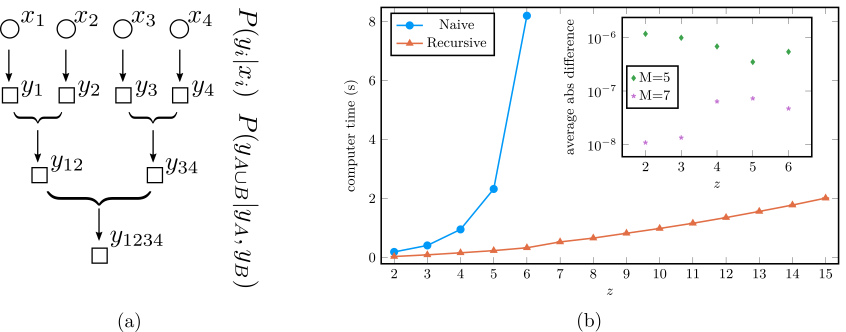
Figure S1: (a) Sketch of the recursive procedure described in this section. (b) Computer time to run 10 iterations of MPBP with the naive vs recursive update for a SIS model on a star graph of degree $z$, $\lambda=0.2,\rho=0.1,\gamma=0.05$, no reweighting, bond dimension $5$, average over $20$ random instances. Error bars are smaller than the points. Inset: absolute difference between values of the marginals for the two methods, averaged over epochs, sites and instances, for two values of bond dimension. Such very small discrepancies are due to the fact that the recursive update, unlike the naive one, performs truncations at each intermediate step.

For the SIS model (SIRS behaves analogously) we pick $y_{A}^{t}$ to be the event that at least one of $k\in A$ infects $i$:

$$p\left(y_{k}^{t}|x_{k}^{t},x_{i}^{t}\right) =\begin{cases}\lambda_{ki}\delta(y_{j}^{t},I)+(1-\lambda_{ki})\delta(y_{k}^{t},S)&\text{if }x_{k}^{t}=S\\ \delta(y_{k}^{t},S)&\text{otherwise }\end{cases}$$ (S39)

$$p\left(y_{A\cup B}^{t}|y_{A}^{t},y_{B}^{t},x_{i}^{t}\right) =\delta(y_{A\cup B}^{t},I)\mathds{1}\left[y_{A}^{t}=I\vee y_{B}^{t}=I\right]+\delta(y_{A\cup B}^{t},S)\mathds{1}\left[y_{A}^{t}=S\wedge y_{B}^{t}=S\right]$$ (S40)

where $\mathds{1}\left[\mathcal{P}\right]$ is the indicator function which evaluates to $1$ when predicate $\mathcal{P}$ is true, to $0$ otherwise.

In this case, all $y$ variables are binary, yielding a computational cost $\mathcal{O}(zM^{6})$ for the update of $z$ messages.

In the case of parallel Glauber dynamics the most general setting where these simplifications apply is couplings with constant absolute value $\left|J_{ij}\right|\equiv J$ and arbitrary external fields, often referred to as the $\pm J$ Ising model. The case with $J_{ij}\equiv J$, $h=0$ studied in [9] is automatically covered. The transition probability (4) takes the form

$$e^{\beta\sigma_{i}^{t+1}\left[J\left(\sum_{j\in\partial i}\operatorname{sign}(J_{ij})\sigma_{j}^{t}\right)+h_{i}\right]} \propto e^{\beta\sigma_{i}^{t+1}\left[J\left(y_{\partial i\setminus j}^{t}+\operatorname{sign}(J_{ij})\sigma_{j}^{t}\right)+h_{i}\right]}$$ (S41)

with $y_{A}^{t}=\sum_{k\in A}\operatorname{sign}(J_{ik})\sigma_{k}^{t}$. It is easy to see that $p\left(y_{\{k\}}^{t}|\sigma_{k}^{t},\sigma_{i}^{t}\right)=\delta\left(y_{\{k\}}^{t},\operatorname{sign}(J_{ik})\sigma_{k}^{t}\right)$ and $p\left(y_{A\cup B}^{t}|y_{A}^{t},y_{B}^{t},\sigma_{i}^{t}\right)=\delta\left(y_{A\cup B}^{t},y_{A}^{t}+y_{B}^{t}\right)$. In this case, $y_{A}^{t}$ can take value $-|A|,-|A|+2,\ldots,|A|-2,|A|$, for a total $2|A|+1$ values. The maximum is achieved for $A=\partial i\setminus j$, yielding a computational cost $\mathcal{O}(z^{2}M^{6})$ for the update of $z$ messages.

VII Population dynamics

For systems with homogeneous properties (e.g. Ising model on a regular graph with homogeneous coupling constant $J_{ij}\equiv J$ and external field $h_{i}\equiv h$), efficient computations in the thermodynamic limit $N\to\infty$ are possible (see e.g. fig. 4(a)). Messages living on each edge of the graph asymptotically become all equal, therefore it is enough to store a single message. This is a standard approach within the cavity method [38] and has been used also in [9]. Whenever the node degree or other parameters of the system are distributed according to some disorder, such a simple approach is not viable. The standard strategy in these cases is to work with a finite collection of BP messages playing the role of a discretized approximation to the true distribution of messages within the disorder ensemble. The approach is called population dynamics [38] and has been used in this paper to produce the data in figure 4(b) where the node degree is randomly distributed.

A population of $P$ messages in matrix-product form (13) is initialized at random. Then, the following is iterated a sufficiently large number $N_{it}$ of times as follows. At each iteration, a degree $z$ is sampled from the degree distribution, then $z$ messages are picked at random from the population. At this point one can imagine a node with $z$ neighbors and the picked messages incoming through the $z$ edges. The outgoing messages are computed according to the BP equation (7), with SVD truncations to some fixed bond dimension. With little further computational effort, the belief (marginal probability distribution (23)) and possibly other observables are also calculated and stored. The newly computed messages are then inserted into the population replacing the ones used as incoming. After $N_{it}$ such iterations, the output of the algorithm is the statistics over the stored observables. Care must be taken in selecting only the samples collected after a stationary state has been reached, i.e. when the population had converged to a good representation of the target probability distribution.

The whole procedure can be run multiple times with increasing bond dimension to verify whether a better approximation can be achieved with larger matrices. The bond dimension is in principle allowed to vary also within the iterations.

A pseudo-code implementation for Glauber dynamics on an infinite Erdos-Renyi graph is provided in algorithm 2.

Algorithm 2 Population dynamics for Glauber dynamics on infinite Erdos-Renyi graph, pseudo-code

$\boldsymbol{m}$: array of $P$ randomly-initialized messages

$\boldsymbol{\tilde{m}}$: auxiliary array of messages for intermediate calculations

$p(z)$: residual degree distribution (Poisson)

$N_{it}$: number of iterations

$M$: max bond dimension for SVD truncations

for $it\in\{1,2,\ldots,N_{it}\}$ do

     sample $z\sim p(z)$

     sample $i_{1},i_{2},\ldots,i_{z}$ from $\{1,2,\ldots,P\}$

     for $j\in\{i_{1},i_{2},\ldots,i_{z}\}$ do

         $\tilde{m}_{j}\leftarrow f_{BP}(\boldsymbol{m}_{\{i_{1},i_{2},\ldots,i_{z}\}\setminus j})$, truncations to size $M$ $\triangleright$ $f_{BP}$ is (7)

     end for

     for $j\in\{i_{1},i_{2},\ldots,i_{z}\}$ do

         $m_{j}\leftarrow\tilde{m}_{j}$

     end for

     store $b=f_{\rm belief}(\boldsymbol{m}_{\{i_{1},i_{2},\ldots,i_{z}\}})$ $\triangleright$ $f_{\rm belief}$ is (23)

end for

Output: average over the stored beliefs, used to estimate average magnetization and autocovariance

VIII Discretized mean-field methods

We report the expressions for the discretized version of Dynamic Message Passing (DMP), Individual-Based Mean Field (IBMF) and Cavity Master Equation (CME) which were used to produce the data in fig. 1. They consist in a discrete time evolution for the expectation of single-variable marginals and cavity marginals (DMP and CME). In the limit of infinitesimal time-step, they reduce to their continuous counterparts. Define $I_{i}^{t}$ as the probability of individual $i$ being in state $I$ at time $t$, $I_{i\to j}^{t}$ ($(ij)\in E$) the probability of individual $i$ being in state $I$ at time $t$ and having been infected by someone other than $j$. We parametrize transmission and recovery probabilities as a rate $\lambda,\rho$ times the time-step $\Delta t$ so that in the continuous-time limit, the equations in their original version are recovered in terms of rates.

For IBMF we have

$$I_{i}^{t+\Delta t}=(1-\rho_{i}\Delta t)I_{i}^{t}+\left(1-\prod_{j\in\partial i}(1-\lambda_{ji}\Delta tI_{j}^{t})\right)(1-I_{i}^{t})$$ (S42)

for DMP

$$I_{i}^{t+\Delta t} =(1-\rho_{i}\Delta t)I_{i}^{t}+\left(1-\prod_{j\in\partial i}(1-\lambda_{ji}\Delta tI_{j\to i}^{t})\right)(1-I_{i}^{t})$$ (S43)

$$I_{i\to j}^{t+\Delta t} =(1-\rho_{i}\Delta t)I_{i\to j}^{t}+\left(1-\prod_{k\in\partial i\setminus j}(1-\lambda_{ki}\Delta tI_{k\to i}^{t})\right)(1-I_{i}^{t})$$ (S44)

and for CME

$$I_{i}^{t+\Delta t} =(1-\rho_{i}\Delta t)I_{i}^{t}+\left(1-\prod_{j\in\partial i}(1-\lambda_{ji}\Delta tI_{j\to i}^{t})\right)(1-I_{i}^{t})$$ (S45)

$$I_{i\to j}^{t+\Delta t} =(1-\rho_{i}\Delta t)I_{i\to j}^{t}+\left(1-\prod_{k\in\partial i\setminus j}(1-\lambda_{ki}\Delta tI_{k\to i}^{t})\right)(1-I_{i\to j}^{t})$$ (S46)

IX Exact mappings

We show examples of models which can be represented exactly by a MPS.

Models with mass on a finite support

Any arbitrary distribution $p(\overline{x})=p(x^{0},x^{1},\ldots,x^{T})$ can in principle be represented via a MPS, albeit with bond dimension exponentially large in $T$: to see this, re-write $p$ trivially as a superposition of delta distributions

$$p(\overline{x})=\sum_{\overline{y}}p(\overline{y})\prod_{t=0}^{T}\delta\left(x^{t},y^{t}\right)$$ (S47)

where the product over $t$ is interpreted as a product of $1\times 1$ matrices. Since the linear combination of two MPSs is itself a MPS [28]:

$$a\prod_{t}A^{t}(x^{t})+b\prod_{t}B^{t}(x^{t})=\prod_{t}C^{t}(x^{t})$$ (S48)

with

$$C^{0}(x^{0})=\left[\begin{array}[]{cc}aA^{0}(x^{0})&bB^{0}(x^{0})\end{array}\right],\quad C^{t}(x^{t})=\left[\begin{array}[]{cc}A^{t}(x^{t})&0\\ 0&B^{t}(x^{t})\end{array}\right],\quad C^{T}(x^{T})=\left[\begin{array}[]{c}A^{T}(x^{T})\\ B^{T}(x^{T})\end{array}\right]$$ (S49)

then $p$ can be expressed by a MPS with bond dimension $q^{T}$, $q$ being the number of values taken by each $x^{t}$. Now, if the distribution under consideration puts non-zero probability only over a small set $\mathcal{T}$ of trajectories, the number of components in the superposition, and hence the final bond dimension, is $|\mathcal{T}|.$

Any non-recurrent and Markovian model with $q$ states such as SIR (Susceptible Infectious Recovered, $q=3$), SEIR (Susceptible Exposed Infectious Recovered, $q=4$), etc., allows only a sub-exponential fraction of the $q^{T}$ potential trajectories. Take as an example the SIR model: each message $m_{i\to j}$ can be parametrized by the infection and recovery times for individuals $i$ and $j$, for a total $\mathcal{O}(T^{4})$ possible trajectories. The same reasoning goes for a generic non-recurrent Markovian model with $q$ states, yielding bond dimension $\mathcal{O}(T^{q^{2}})$.

Chain models

Consider $T+1$ variables each taking one in $q$ values whose distribution is factorized over an open chain

$$p(x^{0},x^{1},\ldots,x^{T})\propto\prod_{i=0}^{T-1}\psi^{t}(x^{t},x^{t+1}).$$ (S50)

We show that there exists an equivalent formulation in MPS form, with matrices of size $q\times q$. Introduce additional variables $\{a^{t}\}_{t=1:T}$with $a^{t}=x^{t}$ to get

$$p(x^{1},x^{2},\ldots,x^{T}) \propto\sum_{a^{1},a^{2},\ldots,a^{T}}\delta(x^{0},a^{1})\prod_{t=0}^{T-2}\left\{\psi^{t}(a^{t+1},x^{t+1})\delta(x^{t+1},a^{t+2})\right\}\psi^{T-1}(a^{T},x^{T})$$ (S51)

$$\propto\sum_{a^{1},a^{2},\ldots,a^{T}}\left[A^{0}(x^{0})\right]_{a^{1}}\prod_{t=1}^{T-1}\left[A^{t}(x^{t})\right]_{a^{t},a^{t+1}}\left[A^{T}(x^{T})\right]_{a^{T}}$$ (S52)

$$\propto\prod_{t=0}^{T}A^{t}(x^{t})$$ (S53)

with

$$\begin{cases}\left[A^{0}(x^{0})\right]_{a^{1}}&=\delta(x^{0},a^{1})\\ \left[A^{t}(x^{t})\right]_{a^{t},a^{t+1}}&=\psi^{t-1}(a^{t},x^{t})\delta(x^{t},a^{t+1})\\ \left[A^{N}(x^{T})\right]_{a^{N}}&=\psi^{T-1}(a^{T},x^{T})\end{cases}\quad\forall t\in 1,2,\ldots,T-1$$ (S54)

where each $a$ ranges over $q$ values. We note the following implication: messages in the $1$-step DMP method Del Ferraro and Aurell [3], which are parametrized as chain models, can be represented with matrices of size $q^{2}\times q^{2}$.

One-particle trajectories in the SI model

We show that the probability of any trajectory of an individual in the SI model can be represented by a MPS with matrices of size $2\times 2$. It suffices to show that such probability factorizes over a chain. In the following we will sometimes use the convention $S=0,I=1$. The rule that once an individual $i$ is infected at time $t$ it can never recover is then encoded compactly as $\prod_{t=1}^{T}\mathds{1}\left[x_{i}^{t+1}\geq x_{i}^{t}\right]$.

For a generic time $t$ consider the conditional probability $p(x^{t+1}|x^{0},x^{1},\ldots,x^{t})$. If $x^{t}=I$ then $p(x^{t+1}|x^{0},x^{1},\ldots,x^{t})=\delta(x^{t+1},I)$. If $x^{t}=S$ then it must also be that $x^{0}=x^{1}=\ldots=x^{t-1}=S$. We conclude that the state at time $t+1$ depends on the previous states only through the state at time $t$: $p(x^{t+1}|x^{0},x^{1},\ldots,x^{t})=p(x^{t+1}|x^{t})$. Hence,

$$p(x^{0},x^{1},\ldots,x^{N})=\prod_{t=0}^{T-1}p(x^{t+1}|x^{0},x^{1},\ldots,x^{t})=\prod_{t=0}^{T-1}p(x^{t+1}|x^{t})$$ (S55)

The same thesis can be proven via a different argument: for “non-recurrent” models like SI, information about the trajectory can be encoded into a single parameter: the infection time. Infection at some time $t_{i}\in\{0,1,\ldots,T,\infty\}$ (we use the convention that no infection corresponds to $t=\infty$) corresponds to $x^{0}=\ldots=x^{t-1}=S,x^{t}=\ldots,x^{T}=I$. It is sometimes convenient to switch between these two equivalent representations.

We propose a chain-factorized ansatz and show that it fully specifies the probability of a trajectory

$$p(x^{0},x^{1},\ldots,x^{T})=\left[\prod_{t=0}^{T-1}\mathds{1}\left[x^{t}\leq x^{t+1}\right]q^{t}(x^{t})\right]q^{T}(x^{T}).$$ (S56)

The probability of any of the allowed trajectories is

$$p(t_{i}=t)=p(x^{0}=\ldots=x^{t-1}=S,x^{t}=\ldots,x^{T}=I)=\prod_{t=0}^{t-1}q^{t}(S)\prod_{t=t}^{T}q^{t}(I).$$ (S57)

The ratio of probabilities of infection at times $t+1$ and $t$ gives

$$\frac{p(t_{i}=t+1)}{p(t_{i}=t)}=\frac{q^{t}(S)}{q^{t}(I)}.$$ (S58)

Parametrizing as $q^{t}(S)\propto 1,q^{t}(I)\propto e^{-h^{t}}$, we get

$$h^{t}=\log\frac{q^{t}(S)}{q^{t}(I)}=\log\frac{p(t_{i}=t+1)}{p(t_{i}=t)}.$$ (S59)

In full detail, the resulting MPS is

$$\begin{cases}\left[A^{0}(x^{0})\right]_{a^{1}}&=\delta(x^{0},a^{1})\\ \left[A^{t}(x^{t})\right]_{a^{t},a^{t+1}}&=\mathds{1}\text{$\left[a^{t}\leq x^{t}\right]$}q^{t-1}(a^{t})\delta(x^{t},a^{t+1})\quad\forall t\in 1,\ldots,T-1\\ \left[A^{T}(x^{T})\right]_{a^{T}}&=\mathds{1}\text{$\left[a^{T}\leq x^{T}\right]$}q^{T-1}(a^{T})q^{T}(x^{T})\end{cases}$$ (S60)

Pair trajectories in the SI model

We show that any BP message in the SI model can be represented exactly by a MPS with matrices of size $6\times 6$. Consider the BP equations for the SI model parametrized with infection times (see [39])

$$m_{i\to j}(t_{i},t_{j}) \propto\sum_{t_{\partial i\setminus j}}\delta\left(t_{i},\min_{k\in\partial i}\left\{t_{k}\right\}\right)\prod_{k\in\partial i\setminus j}m_{k\to i}(t_{k},t_{i})$$ (S61)

$$\propto\mathds{1}\left[t_{i}\leq t_{j}\right]\prod_{k\in\partial i\setminus j}\sum_{t_{k}}\mathds{1}\left[t_{i}\leq t_{k}\right]m_{k\to i}(t_{k},t_{i})-\mathds{1}\left[t_{i}<t_{j}\right]\prod_{k\in\partial i\setminus j}\sum_{t_{k}}\mathds{1}\left[t_{i}<t_{k}\right]m_{k\to i}(t_{k},t_{i})$$ (S62)

$$\propto\mathds{1}\left[t_{i}\leq t_{j}\right]a_{i\to j}(t_{i})-\mathds{1}\left[t_{i}<t_{j}\right]b_{i\to j}(t_{i})$$ (S63)

$$\propto\mathds{1}\left[t_{i}\leq t_{j}\right]c_{i\to j}(t_{i})+\mathds{1}\left[t_{i}=t_{j}\right]b_{i\to j}(t_{i})$$ (S64)

where we used $\delta\left(x,\min_{k\in S}\left\{x_{k}\right\}\right)=\prod_{k\in S}\mathds{1}\left[x\leq x_{k}\right]-\prod_{k\in S}\mathds{1}\left[x<x_{k}\right]$ and defined $a_{i\to j}(t_{i})=\prod_{k\in\partial i\setminus j}\sum_{t_{k}}\mathds{1}\left[t_{i}\leq t_{k}\right]m_{k\to i}(t_{k},t_{i})$, $b_{i\to j}(t_{i})=\prod_{k\in\partial i\setminus j}\sum_{t_{k}}\mathds{1}\left[t_{i}<t_{k}\right]m_{k\to i}(t_{k},t_{i})$, $c_{i\to j}(t_{i})=a_{i\to j}(t_{i})-b_{i\to j}(t_{i})$.

Once normalized, both $c_{i\to j}$ and $b_{i\to j}$ are probability distributions for a single SI trajectory, hence they can be re-parametrized (with a slight abuse of notation) as MPSs $c_{i\to j}(x_{i})=\prod_{t}\mathds{1}\left[x_{i}^{t+1}\geq x_{i}^{t}\right]\tilde{c}_{i\to j}^{t}(x_{i}^{t})$, $b_{i\to j}(x_{i})=\prod_{t}\mathds{1}\left[x_{i}^{t+1}\geq x_{i}^{t}\right]\tilde{b}_{i\to j}^{t}(x_{i}^{t})$. Introducing the SI rule also for $x_{j},$we get

$$m_{i\to j}(x_{i},x_{j})\propto\prod_{t}\mathds{1}\left[x_{i}^{t}=x_{j}^{t}\right]\mathds{1}\left[x_{i}^{t+1}\geq x_{i}^{t}\right]\tilde{b}_{i\to j}(x_{i})+\prod_{t}\mathds{1}\left[x_{i}^{t}\leq x_{j}^{t}\right]\mathds{1}\left[x_{i}^{t+1}\geq x_{i}^{t}\right]\mathds{1}\left[x_{j}^{t+1}\geq x_{j}^{t}\right]\tilde{c}_{i\to j}^{t}(x_{i}^{t}).$$ (S65)

The first term is a chain-factorized distribution for, say, $x_{i}$ times the constraint $x_{j}^{t}=x_{i}^{t}\forall t$, hence it can be represented as an MPS with $2\times 2$ matrices. The second term is a chain of $4$-state variables $\{(x_{i}^{t},x_{j}^{t})\}_{t=0:T}$, hence it can be represented as an MPS with $4\times 4$ matrices. In full detail

$$\prod_{t}\mathds{1}\left[x_{i}^{t}=x_{j}^{t}\right]\mathds{1}\left[x_{i}^{t+1}\geq x_{i}^{t}\right]\tilde{b}_{i\to j}(x_{i})=\sum_{a_{i}^{1},\ldots,a_{i}^{T}}\prod_{t}\underbrace{\mathds{1}\left[x_{i}^{t}=x_{j}^{t}\right]\delta(x_{i}^{t},a_{i}^{t+1})\mathds{1}\left[a_{i}^{t}\leq x_{i}^{t}\right]\tilde{b^{t-1}}_{i\to j}(a_{i}^{t})}_{\left[B^{t}(x_{i}^{t},x_{j}^{t})\right]_{a_{i}^{t},a_{i}^{t+1}}}$$ (S66)

$$\prod_{t}\mathds{1}\left[x_{i}^{t}\leq x_{j}^{t}\right]\mathds{1}\left[x_{i}^{t+1}\geq x_{i}^{t}\right]\mathds{1}\left[x_{j}^{t+1}\geq x_{j}^{t}\right]\tilde{c}_{i\to j}^{t}(x_{i}^{t})=\sum_{\begin{subarray}{c}a_{i}^{1},\ldots,a_{i}^{T}\\ a_{j}^{1},\ldots,a_{j}^{T}\end{subarray}}\prod_{t}\underbrace{\mathds{1}\left[x_{i}^{t}\leq x_{j}^{t}\right]\delta(x_{i}^{t},a_{i}^{t+1})\delta(x_{j}^{t},a_{j}^{t+1})\mathds{1}\left[a_{i}^{t}\leq x_{i}^{t}\right]\mathds{1}\left[a_{j}^{t}\leq x_{j}^{t}\right]\tilde{c}_{i\to j}^{t-1}(a_{i}^{t})}_{\left[C^{t}(x^{t})\right]_{(a_{i}^{t},a_{j}^{t}),(a_{i}^{t+1},a_{j}^{t+1})}}$$ (S67)

Finally, since the mixture of two MPSs is itself an MPS (S48), we get that $m_{i\to j}$ can be written as a MPS with matrices of size $2+4=6$.

X Pair-wise reweightings

The distribution (2) can be made more general by adding reweighting terms involving neighboring variables $\left\{\psi_{ij}^{t}(x_{i}^{t},x_{j}^{t})\right\}_{(ij)\in E}$. Now

$$\begin{aligned} p(\overline{\boldsymbol{x}})\propto&\prod_{i=1}^{N}w(x_{i}^{0})\prod_{t=0}^{T-1}\prod_{i=1}^{N}w(x_{i}^{t}|\boldsymbol{x}_{\partial i}^{t-1},x_{i}^{t-1})\phi_{i}^{t}(x_{i}^{t})\prod_{(ij)}\psi_{ij}^{t}(x_{i}^{t},x_{j}^{t})\end{aligned}.$$ (S68)

The message ansatz stays the same. The BP equation becomes

$$m_{i\to j}(\overline{x}_{i},\overline{x}_{j})\propto\sum_{\overline{x}_{\partial i\setminus j}}w(x_{i}^{0})\phi_{i}^{0}(x_{i}^{0})\prod_{t}w(x_{i}^{t+1}|\boldsymbol{x}_{\partial i}^{t},x_{i}^{t})\phi_{i}^{t+1}(x_{i}^{t+1})\prod_{k\in\partial i\setminus j}\psi_{ik}^{t+1}(x_{i}^{t+1},x_{k}^{t+1})\prod_{k\in\partial i\setminus j}m_{k\to i}(\overline{x}_{k},\overline{x}_{i})$$ (S69)

and the $B$ matrices read

$$\left[B_{i\to j}^{0}(x_{i}^{1},x_{i}^{0},x_{j}^{0})\right]_{\{a_{k}^{1}\}_{k\in\partial i\setminus j}} =w(x_{i}^{0})\phi_{i}^{0}(x_{i}^{0})\sum_{\{x_{k}^{0}\}_{k\in\partial i\setminus j}}w(x_{i}^{1}|\boldsymbol{x}_{\partial i}^{0},x_{i}^{0})\prod_{k\in\partial i\setminus j}\psi_{ij}^{0}(x_{k}^{0},x_{i}^{0})\left[A_{k\to i}^{0}(x_{k}^{0},x_{i}^{0})\right]_{a_{k}^{1}}$$ (S70)

$$\left[B_{i\to j}^{t}(x_{i}^{t+1},x_{i}^{t},x_{j}^{t})\right]_{\{a_{t}^{k},a_{t+1}^{k}\}_{k\in\partial i\setminus j}} =\phi_{i}^{t}(x_{i}^{t})\sum_{\{x_{k}^{t}\}_{k\in\partial i\setminus j}}w(x_{i}^{t+1}|\boldsymbol{x}_{\partial i}^{t},x_{i}^{t})\prod_{k\in\partial i\setminus j}\psi_{ik}^{t}(x_{k}^{t},x_{i}^{t})\left[A_{i\to j}^{t}(x_{i}^{t},x_{j}^{t})\right]_{a_{k}^{t},a_{k}^{t+1}}$$

$$\quad\forall t\in\{1,\ldots,T-1\}$$

$$\left[B_{i\to j}^{T}(x_{i}^{T},x_{j}^{T})\right]_{\{a_{k}^{T}\}_{k\in\partial i\setminus j}} =\phi_{i}^{T}(x_{i}^{T})\sum_{\{x_{k}^{T}\}_{k\in\partial i\setminus j}}\prod_{k\in\partial i\setminus j}\psi_{ik}^{T}(x_{i}^{T},x_{k}^{T})\left[A_{k\to i}^{T}(x_{k}^{T},x_{i}^{T})\right]_{a_{k}^{T}}.$$

References

• Van Mieghem et al. [2008] P. Van Mieghem, J. Omic,  and R. Kooij, IEEE/ACM Transactions On Networking 17, 1 (2008).
• Karrer and Newman [2010] B. Karrer and M. E. Newman, Physical Review E 82, 016101 (2010).
• Del Ferraro and Aurell [2015] G. Del Ferraro and E. Aurell, Phys. Rev. E 92, 010102 (2015).
• Pelizzola [2013] A. Pelizzola, The European Physical Journal B 86, 1 (2013).
• Pelizzola and Pretti [2017] A. Pelizzola and M. Pretti, Journal of Statistical Mechanics: Theory and Experiment 2017, 073406 (2017).
• Aurell et al. [2017] E. Aurell, G. Del Ferraro, E. Domínguez,  and R. Mulet, Phys. Rev. E 95, 052119 (2017).
• Ortega et al. [2022] E. Ortega, D. Machado,  and A. Lage-Castellanos, Phys. Rev. E 105, 024308 (2022).
• Neri and Bollé [2009] I. Neri and D. Bollé, Journal of Statistical Mechanics: Theory and Experiment 2009, P08009 (2009).
• Barthel et al. [2018] T. Barthel, C. De Bacco,  and S. Franz, Physical Review E 97, 010104 (2018).
• Barthel [2020] T. Barthel, Journal of Statistical Mechanics: Theory and Experiment 2020, 013217 (2020).
• Perez-Garcia et al. [2007] D. Perez-Garcia, F. Verstraete, M. M. Wolf,  and J. I. Cirac, Quantum Info. Comput. 7, 401 (2007).
• Verstraete and Cirac [2006] F. Verstraete and J. I. Cirac, Physical review b 73, 094423 (2006).
• Fannes et al. [1992] M. Fannes, B. Nachtergaele,  and R. F. Werner, Communications in mathematical physics 144, 443 (1992).
• Derrida et al. [1993] B. Derrida, M. R. Evans, V. Hakim,  and V. Pasquier, Journal of Physics A: Mathematical and General 26, 1493 (1993).
• Bañuls and Garrahan [2019] M. C. Bañuls and J. P. Garrahan, Physical review letters 123, 200601 (2019).
• Han et al. [2018] Z.-Y. Han, J. Wang, H. Fan, L. Wang,  and P. Zhang, Physical Review X 8, 031012 (2018).
• Stoudenmire and Schwab [2016] E. Stoudenmire and D. J. Schwab, Advances in neural information processing systems 29 (2016).
• Altarelli et al. [2013] F. Altarelli, A. Braunstein, L. Dall’Asta,  and R. Zecchina, Physical Review E 87, 062115 (2013).
• Crotti and Braunstein [2023] S. Crotti and A. Braunstein, “MatrixProductBP,” https://github.com/stecrotti/MatrixProductBP.jl (2023), accessed 27/10/2023.
• Renart et al. [2010] A. Renart, J. De La Rocha, P. Bartho, L. Hollender, N. Parga, A. Reyes,  and K. D. Harris, science 327, 587 (2010).
• Roudi and Hertz [2011] Y. Roudi and J. Hertz, Physical review letters 106, 048702 (2011).
• Ohta and Sasa [2010] H. Ohta and S.-i. Sasa, Europhysics Letters 90, 27008 (2010).
• Van Mieghem [2011] P. Van Mieghem, Computing 93, 147 (2011).
• Shrestha et al. [2015] M. Shrestha, S. V. Scarpino,  and C. Moore, Physical Review E 92, 022821 (2015).
• Vázquez et al. [2017] E. D. Vázquez, G. Del Ferraro,  and F. Ricci-Tersenghi, Journal of Statistical Mechanics: Theory and Experiment 2017, 033303 (2017).
• Del Ferraro and Aurell [2014] G. Del Ferraro and E. Aurell, Journal of the Physical Society of Japan 83, 084001 (2014).
• Antulov-Fantulin et al. [2015] N. Antulov-Fantulin, A. Lančić, T. Šmuc, H. Štefančić,  and M. Šikić, Physical review letters 114, 248701 (2015).
• Oseledets [2011] I. V. Oseledets, SIAM Journal on Scientific Computing 33, 2295 (2011).
• [29] J. Kunegis, “Zachary karate club,” http://konect.cc/networks/ucidata-zachary/, accessed: 14.01.2023.
• Coja-Oghlan et al. [2022] A. Coja-Oghlan, P. Loick, B. F. Mezei,  and G. B. Sorkin, SIAM Journal on Discrete Mathematics 36, 1306 (2022).
• Iba [1999] Y. Iba, Journal of Physics A: Mathematical and General 32, 3875 (1999).
• Yedidia et al. [2000] J. S. Yedidia, W. Freeman,  and Y. Weiss, Advances in neural information processing systems 13 (2000).
• Schollwöck [2011] U. Schollwöck, Annals of physics 326, 96 (2011).
• Larsen [1998] R. M. Larsen, DAIMI Report Series  (1998).
• Baglama and Reichel [2005] J. Baglama and L. Reichel, SIAM Journal on Scientific Computing 27, 19 (2005).
• Glauber [1963] R. J. Glauber, Journal of mathematical physics 4, 294 (1963).
• Peretto [1984] P. Peretto, Biological cybernetics 50, 51 (1984).
• Mezard and Montanari [2009] M. Mezard and A. Montanari, Information, physics, and computation (Oxford University Press, 2009).
• Altarelli et al. [2014] F. Altarelli, A. Braunstein, L. Dall’Asta, A. Lage-Castellanos,  and R. Zecchina, Physical review letters 112, 118701 (2014).