A Quantization Procedure for Nonlinear Pricing with an Application to Electricity Markets

Abstract

We consider a revenue maximization model, in which a company aims at designing a menu of contracts, given a population of customers. A standard approach consists in constructing an incentive-compatible continuum of contracts, i.e., a menu composed of an infinite number of contracts, where each contract is especially adapted to an infinitesimal customer, taking his type into account. Nonetheless, in many applications, the company is constrained to offering a limited number of contracts. We show that this question reduces to an optimal quantization problem, similar to the pruning problem that appeared in the max-plus based numerical methods in optimal control. We develop a new quantization algorithm, which, given an initial menu of contracts, iteratively prunes the less important contracts, to construct an implementable menu of the desired cardinality, while minimizing the revenue loss. We apply this algorithm to solve a pricing problem with price-elastic demand, originating from the electricity retail market. Numerical results show an improved performance by comparison with earlier pruning algorithms.

I INTRODUCTION

I-A Motivation from electricity markets

Electricity retail markets are now open to competition in most countries, and providers are free to design a menu of offers/contracts in addition to regulated alternatives (fixed prices), so that each consumer can select among the vast jungle of offers the one which maximizes his utility. Finding an appropriate utility function which fairly represents the consumer behavior is all but immediate. In this paper, the choice of a contract is based on the minimization of the invoice (rational choice theory, see e.g. [1]), and we suppose that each customer can adjust his consumption to the electricity prices (price elasticity). This phenomenon is highlighted by the actual energy crisis: consumers are likely to make huge efforts in view of consumption reduction.

A key problem for electricity providers is to design an optimal menu of offers, maximizing their revenue, under a restriction on the “size” of the menu (number of contracts). In fact, from an optimization point of view, proposing more contracts increases the revenue, as it allows one to adjust the menu to the individual preferences of the different types of customers. However, in practice, it is essential to restrict the number of contracts, in order to make the commercial offer more visible to agents, easier to understand, and also to keep an implementable menu for the company.

I-B The optimal nonlinear pricing problem

We consider more generally the revenue maximization problem faced by a seller, called principal, or leader in the setting of Stackelberg games [2]. This problem has been addressed by the theory of mechanism design [3] through the question of nonlinear pricing. The so-called monopolist problem is among the most studied ones: in this approach, the population is represented as a continuum of buyers (called agents or followers), and a contract can be specifically designed for each agent (continuum menu). In the seminal paper [4], Rochet and Choné study the monopolist problem by introducing a dual approach. In some specific cases (linear-quadratic setting and specific agents distribution), analytic solutions can be found in one [5] or many dimensions [6], via reformulation as welfare maximization using virtual valuation technique. Extending the framework of Rochet and Choné to decomposable variational problem under convexity requirement, Carlier [7] addresses the question of the existence and uniqueness of a solution, and proposes an iterative algorithm. In the specific case $\operatorname{\mathbb{R}}^{2}$, Mirebeau [8] introduces a more efficient method using an adaptive mesh based on stencils. The infinite-size menu is therefore characterized by a value-function satisfying the incentive-compatibility conditions as with the full-participation condition, the latter supposing that contracting with the whole population is optimal. Bergemann, Yeh and Zhang recently considered the question of the optimal quantization of a menu [9].

I-C Contributions

Our main contribution is the development of new quantization algorithms which, given the infinite-size menu, aim at finding the best $n$-contracts approximation that maximizes the revenue. This 2-step strategy bypasses the combinatorial difficulty tackled in bilevel pricing – see e.g. [10, 11] – where formulations directly embed customer choices over the $n$ contracts, becoming rapidly untractable for large size of menu. We show that the quantization problem is equivalent to the pruning problem, which arose, following McEneaney [12], in the development of the max-plus based curse-of-dimensionality attenuation methods in numerical optimal control, see [13, 14, 15], and [16] for an application. In these methods, the value function of an optimal control problem is represented as a supremum of “basis functions”, and one looks for a sparse representation – with a prescribed number of basis functions. In the present application, the basis functions are linear functions, representing contracts. We develop a greedy descent algorithm which iteratively removes the less “important” contracts. We consider different importance measures, taking into account the $L_{1}$ and $L_{\infty}$ approximation errors previously considered in the study of the pruning problem, and also a specific measure of the loss of revenue, see Algorithms 1 and 2. An essential feature of these algorithms is the low incremental cost per iteration, with an update rule requiring only local computations – in a “small neighborhood” of the active set of a basis function. To do so, we exploit discrete geometry techniques, by associating to a basis decomposition a polyhedral complex, which is updated dynamically.

To apply this algorithm to the optimal design of a menu in the electricity retail market, we generalize the framework of [7] to allow for a nondecomposable (still convex) cost. Indeed, the revenue of the provider depends on the furniture cost, supposed to be an increasing function of the global consumption, see e.g. ([17, 18]). In this extended setting, we prove the existence and uniqueness of the solution, see Theorem II.2. The solving of this problem is then tackled by a direct method (discretization of the variational problem). A key feature of the pricing application is the elastic behavior of the customers, who adapt their consumption according to prices. We show that, after an appropriate change of variables, this actually reduces to the previous model, see Theorem IV.1. Numerical tests, on a realistic instance (arising from the French electricity market), illustrate the efficiency of our approach both in terms of revenue gain and of computational time, see Figure 3. Our algorithm also allows one to estimate the minimal admissible number of contracts, given a target level of acceptable revenue loss by comparison with the case of an infinite number of contracts.

I-D Related works

In the nonlinear pricing context, the restriction to a finite number of offers has been regarded only recently. In [9], the authors analyze the loss of revenue induced by this restriction, exhibiting upper bounds of order $1/n^{2/d}$, where $d$ is the dimension and $n$ the maximal number of contracts. A similar asymptotic error rate arose in a different setting of quantization theory, see e.g. [14]. Moreover, in the linear-quadratic setting of [9], the extreme distributions realizing the worst revenue loss satisfies separability conditions à la Armstrong [6], leading to an explicit expression for the optimal quantization. We do not satisfy these requirements here, as we tackle a broader class of variational problem, hence the need of efficient methods to solve the pricing problems with a finite number of contracts. In [19], a discretization is obtained by writing the utility function as a supremum of finitely many affine functions, and so the solution they obtain can be viewed as a $n$-contracts menu. However, the scheme also discretizes the population (with the same size as the contracts). In the present application, this is not desirable, since the size of the population has to be much larger that the size of the menu.

The present algorithms should be compared with the pruning methods to compute a sparse representation of a function as maximum of a prescribed number of basis functions. The pruning problem was shown in [14] to be a continuous version of the facility location problem, a hard combinatorial optimization problem. The pruning algorithms developed in [13, 14] rely on a notion of importance metric, measuring the contribution of each basis function to the approximation error. A basic algorithm in [13, 14] perform a single pass which keeps only the $n$ basis functions with the highest importance metric, the latter being evaluated either by solving a convex programming problem or in approximate way, after a discretization of the state space. A greedy ascent algorithm is also implemented in [14], adding incrementally functions by decreasing order of importance. In contrast, the present algorithm does not require a discretization of the state space. Moreover, the use of fast (local) updates of the importance measure allows us to perform a greedy descent starting from the complete family of basis functions, and removing at each stage the less important one. This leads to improved performances on our application case.

The paper is organized as follows: in Section II, we define the nonlinear pricing problem, adapted to our application case, and encompassing the monopolist framework. In Section III, we approximate the continuum menu by a finite set of contracts, and present refined pruning algorithms with local update. Then, in Section IV, we specify the problem encountered in electricity markets, and show how it boils down to the general case of Section II. Finally, we numerically study the effectiveness of our approach in Section V.

II NONLINEAR PRICING WITH COUPLING COSTS

II-A Notation

For two vectors $x$ and $y$ of $\operatorname{\mathbb{R}}^{d}$, we denote by $\left<x,y\right>$ the scalar product and $x\odot y$ the entrywise product. Moreover, for a discrete set $S$, we denote by $|S|$ the cardinality of $S$.

II-B Generalized monopolist problem

Let us consider a heterogeneous population, where each agent in the population is defined by a $d$-dimensional vector of characteristics $x\in X$. We suppose that $X\subset\operatorname{\mathbb{R}}^{d}_{>0}$ is a compact polyhedral domain. An agent of type $x$ will derive a utility $\left<x,\alpha\odot q_{k}\right>-p_{k}$ from consuming a good $k$ with quality $q_{k}\in\operatorname{\mathbb{R}}^{d}_{>0}$ and price $p_{k}\in\operatorname{\mathbb{R}}_{>0}$. The vector $\alpha\in(\operatorname{\mathbb{R}}^{*})^{d}$ is an exogeneous data rescaling the quality vector. The agents are distributed according to $\rho$ satysfying $\int_{X}\rho(x)\textnormal{d}x=1$.

Let us consider a monopolist (principal) who designs a contract menu represented by a pair of functions $x\mapsto(p(x),q(x))\in P\times Q$. For each agent $x$, these functions indicate respectively the price and the quality that the agent is supposed to prefer. Here, $P$ and $Q$ are compact subsets of $\operatorname{\mathbb{R}}_{>0}$ and $\operatorname{\mathbb{R}}^{d}_{>0}$. To ensure that the contract $(p(x),q(x))$ really satisfies agent of type $x$, an additional constraint on the shape of the function, called incentive-compatibility condition is required: denoting by $u(x):=\left<x,\alpha\odot q(x)\right>-p(x)$ the utility function for the menu designed by the monopolist,

$$~{}u(y)-u(x)\geq\left<y-x,\alpha\odot q(x)\right>,\;\forall x,y\in X\enspace.$$ (1)

Let $U_{x}$ be the set of admissible values of $u$ for type $x$:

$$U_{x}:=\{\left<x,\alpha\odot q\right>-p\mid(p,q)\in P\times Q\}\enspace.$$

Each set $U_{x}$ is compact by compactness of $P$ and $Q$.

Proposition II.1 ([20])

Let $q(\cdot)$ be defined on $X$, with values in $Q$. There exists a function $p:X\to P$ such that $u(\cdot)$ satisfies (1) if and only if

1. $u(x)\in U_{x},$ for $x\in X$,

2. $u$ is convex on $X$,

3. $\nabla u(x)=\alpha\odot q(x)$ for a.e. $x\in X$.

The aim of the monopolist is then to maximize a revenue function, defined as

$$J(u,q):=\int_{X}L(x,u(x),q(x))\textnormal{d}x-C\left(\int_{X}M(x,q(x))\textnormal{d}x\right)\,,$$ (2)

In (2), the cost function $C$ takes as input data aggregated on the whole domain $X$. Such coupling cost naturally appears in some applications, for instance in electricity retail market, see Section IV.

Assumption II.1

The integrand $L$ is linear in $u$ and $q$. Moreover, the integrand $M$ is strictly convex in $q$, and $C$ is increasing and strictly convex.

In addition to the incentive-compatibility condition, the utility must be greater to a reservation utility:

$$u(x)\geq R(x)\enspace.$$ (3)

The problem solved by the monopolist is then

$$\max_{u,q}\left\{J(u,q)\;\left|\begin{split}&u,q\text{ satisfy }\eqref{eq::i_compatibility},\eqref{eq::reservation_utility}\\ &(u(x),q(x))\in U_{x}\times Q\text{ for }x\in X\end{split}\right.\right\}$$ (4)

Theorem II.2

Under II.1, Problem (4) has a unique optimal solution.

The proof of Theorem II.2 is given in Section VII-A. This result should be compared with [21], where the (decomposable) criteria is defined by an integrand that must satisfy coercivity condition, which entails that a minimizing sequence $(u_{n})$ must be bounded in the $W^{1,1}$ Sobolev norm. Here, $J$ is not necessarily coercive. Instead, the compactness argument directly comes with assumptions on $P$ and $Q$.

II-C Resolution of the infinite-size case

As an extension of the monopolist problem, Problem (4) can be solved to optimality through a discretization scheme. In [19], the authors proved the convergence of the discretized problem to the continuous one, which can be extended to nondecomposable cost. Efficient numerical methods have been proposed in [7] and [8]. Let us define a regular grid $\Sigma$ of $X$. Each of the methods provides a solution $\{(\hat{p}_{i},\hat{q}_{i})\}_{i\in\Sigma}$, inducing a convex utility function $\hat{u}_{\Sigma}$ that can be represented as the supremum of affine functions, with the notation:

$$\hat{u}_{S}(x)=\max_{i\in S}\hat{u}_{i}(x),\;S\subseteq\Sigma\enspace,$$ (5)

where $\hat{u}_{i}:x\in\operatorname{\mathbb{R}}^{d}\mapsto\left<\hat{q}_{i},x\right>-\hat{p}_{i}$. In the context of max-plus methods [12, 22], the functions $\hat{u}_{i}$ are called basis functions and can be more general than affine functions, but we focus here on this specific case, as this naturally appears in the model (affine contracts).

III PRUNING PROCEDURES

III-A Pruning method for max-plus basis decomposition

Let us now suppose that the monopolist has a maximal number of $n$ contracts he can design. Given the discretized infinite-size solution $u_{\Sigma}$, the question can be recast as the following combinatorial problem:

$$\min_{S\subseteq\Sigma}\;\left\{d(\hat{u}_{S},\hat{u}_{\Sigma})\text{ s.t. }|S|\leq n\right\}\enspace,$$ (6)

where the function $d(\cdot)$ can be either

1. the $L_{\infty}$ norm $d_{\infty}(u,v)=\left\|u-v\right\|_{L_{\infty}(X)}$,

2. the $L_{1}$ norm $d_{1}(u,v)=\left\|u-v\right\|_{L_{1}(X)}$,

3. and the $J$-based criterion $d_{J}(u,v)=J(v,\alpha^{\scalebox{0.5}[1.0]{$-$}1}\odot\nabla v)-J(u,\alpha^{\scalebox{0.5}[1.0]{$-$}1}\odot\nabla u)\enspace.$

The third case corresponds to the maximization of the function $J$, where $\alpha^{\scalebox{0.5}[1.0]{$-$}1}\odot q=\nabla u$ thanks to II.1.

Theorem III.1 ([14])

Let $X\subseteq\operatorname{\mathbb{R}}^{d}$ and $v:X\to\operatorname{\mathbb{R}}$ strongly convex of class $\operatorname{\mathcal{C}}^{2}$. Then, both $L_{1}$ and $L_{\infty}$ approximation errors are $\Omega\left(\frac{1}{n^{2/d}}\right)$ as $n\to\infty$.

Theorem III.1 exhibits an error rate identical to the complexity bound proved in [9] in a different setting.

We define the importance metric of basis function $i$ as

$$\nu(S,i)=d(\hat{u}_{S\backslash\{i\}},\hat{u}_{S})\enspace.$$ (7)

This corresponds to an incremental version of the criteria (6). For the $L_{\infty}$ and $L_{1}$ case, if $\nu(S,i)=0$, then the $i$-th basis function does not contribute to the max-sum. Otherwise, if $\nu(S,i)>0$, then it expresses the maximal difference between the shape of $\hat{u}_{S}$ with and without $\hat{u}_{i}$, depending on the criterion. For the criterion $d_{J}$, it expresses the loss of revenue for the principal when contract $i$ is removed.

III-B Specific case: minimizing $L_{\infty}$ error

For a $L_{\infty}$ approximation error, the importance metric (7) can be computed by solving a linear program, see [14]:

$$\max_{x\in X,\,\nu} \quad\nu P^{S}_{i}$$ ()

s.t $$\quad\forall j\in S\backslash\{i\},\quad\hat{u}_{i}(x)-\hat{u}_{j}(x)\geq\nu\quad(\lambda_{ij})$$

In ($P^{S}_{i}$), we denote by $(\lambda_{ij})_{j}$ the dual variable associated with each constraint. The set of saturated constraints is then characterized by the positive variables $\lambda_{ij}$.

Algorithm 1 Pruning for $L_{\infty}$ importance metric

1:$n$$\triangleright$ Desired number of contracts

2:$S\leftarrow\Sigma$ $\triangleright$ Indices of kept contracts

3:$I\leftarrow\Sigma$ $\triangleright$ Indices of problems to re-compute

4:for $t=1:|\Sigma|-n$ do

5:    for $i\in I$ do

6:         $\nu_{i},\lambda_{i}\leftarrow$ solution of $(P^{S}_{i})$

7:         $J_{i}\leftarrow\{j\in S\backslash\{i\}\mid\lambda_{ij}>0\}$

8:    end for

9:    $r\leftarrow\operatorname*{arg\,min}_{i\in S}\nu_{i}$ $\triangleright$ Contract to remove

10:    $S\leftarrow S\backslash\{r\}$

11:    $I\leftarrow\{i\in S\mid r\in J_{i}\}$

12:end for

13:return $S$

Algorithm 1 describes a greedy descent procedure: we start from the complete set of contracts $S$, and iteratively remove the less important contract exploiting a fast local update of the importance metric. Compared with [14], we take advantage of the linearity of the basis functions $\hat{u}_{i}$ to exploit the optimal dual variables $\lambda_{ij}$ in the linear program ($P^{S}_{i}$):

Proposition III.2 (Local update)

Let $\lambda_{ij}$ be the optimal dual variables in ($P^{S}_{i}$) for a contract $i\in S$. Then, the importance metric of $i$ stays unchanged when we remove a contract $j\in S$ s.t. $\lambda_{ij}=0$, i.e., $\nu(S\backslash\{j\},i)=\nu(S,i)$.

III.2 ensures the correctness of Algorithm 1, where we only re-compute at each iteration the values $\nu_{i}$ for a very small subset of $\Sigma$. This leads to a huge gain in computation time, see Section V.

III-C $L_{1}$ and $J$-based approximation error

Contrary to the $L_{\infty}$ case, the computation exploits the geometric structure. Indeed, the representation of the function $\hat{u}_{S}$ as a maximum of basis functions’ $\hat{u}_{j},j\in S$ induces a polyhedral complex, in which every function $\hat{u}_{i}$ determines a polyhedral cell $\mathcal{C}_{i}$, consisting of the types $x\in X$ such that $\hat{u}_{S}(x)=\hat{u}_{i}(x)$. Removing a basis function $\hat{u}_{i}$ from the supremum $\hat{u}_{S}=\sup_{j\in S}\hat{u}_{j}$ yields a local modification of the latter supremum, concentrated on a neighborhood of the cell $\mathcal{C}_{i}$. Hence, we will need to compute at each iteration the neighbors of each contract cell $\mathcal{C}_{i}$ with $i\in S$. This idea may be compared with the notion of Delaunay triangulation associated to a Voronoï diagram [23]. During the algorithm, we keep in memory two sets: $J_{i}$ represents the neighboring cells of cell $i$, and $V_{i}$ is the vertex representation of cell $i$. Two routines are used for both the $L_{1}$ and $J$-based criterion:

• Vrep$(S,i)$ returns the V-representation (representation by vertices) of the polyhedral cell $\mathcal{C}_{i}$ induced by contract $i$ for a given set $S$, taking as input the H-representation (representation by half-spaces) $\{x\in X\mid\hat{u}_{i}(x)\geq\hat{u}_{j}(x),\;\forall j\in S\}$ of the cell $i$. This is done using the revised reverse search algorithm implemented in the library lrs, see [24].

• updateNeighbors$((V_{S})_{i\in I})$ updates the neighbors of each cell $i\in I$ knowing the vertex representation.

Proposition III.3 (Local update)

The importance metric of a contract $i\in S$ stays unchanged when we remove a contract $j$ which is not in the neighborhood of $i$, i.e., $\nu(S\backslash\{j\},i)=\nu(S,i)$ for $j\in S\backslash J_{i}$.

III.3 ensures the correctness of Algo. 2, where we only re-compute vertex representations for a small subset of contracts (corresponding to the neighboring cells of the lastly removed contract, see line 8 of the algorithm). This local update is illustrated in Figure 1. The update of the importance metric in line 11 differs between the $L_{1}$ and $J$-based cases, and is described in Algos. 3a–3b. In Algo. 3a, the integral that appears in the computation of $\nu_{i}$ can be evaluated analytically using Green’s formula, as it integrates a linear form over a polytope, see Appendix VII-B. In Algo. 3b, $\delta_{L}$ can be computed in the same way. For $M_{0}$ and $\delta_{M}$, this generally involves the integration of the function $x\mapsto M(x,\hat{q}_{i})$. In the present application, this function is linear, and so the direct integration is possible, see (14)–(15).

Algorithm 2 Pruning with local update (for $L_{1}$ and $J$-based)

1:$n$$\triangleright$ Desired number of contracts

2:for $i\in\Sigma$ do

3:    $V_{i}\leftarrow$ Vrep$(\Sigma,i)$ $\triangleright$ Vertex representation

4:end for

5:$S\leftarrow\Sigma$ $\triangleright$ Indices of kept contracts

6:$I\leftarrow\Sigma$ $\triangleright$ Indices of problems to re-compute

7:for $t=1:|\Sigma|-n$ do

8:    $(J_{i})_{i\in I}\leftarrow$ updateNeighbors$((V_{i})_{i\in I})$

9:    for $i\in I$, $j\in J_{i}$ do

10:         $F_{j,-i}\leftarrow$ Vrep$(S\backslash\{i\},j)$ $\triangleright$ Future cells

11:    end for

12:    $\nu\leftarrow$ updateImpMetric$(I,(V_{i})_{i\in S},(F_{j,\scalebox{0.5}[1.0]{$-$}i})_{j\in J_{i},i\in S})$

13:    $r\leftarrow\operatorname*{arg\,min}_{i\in S}\nu_{i}$ $\triangleright$ Contract to remove

14:    $S\leftarrow S\backslash\{r\}$

15:    for $j\in J_{r}$ do

16:         $V_{j}\leftarrow F_{j,-r}$ $\triangleright$ Update vertex representation

17:    end for

18:    $I\leftarrow J_{r}$

19:end for

20:return $S$

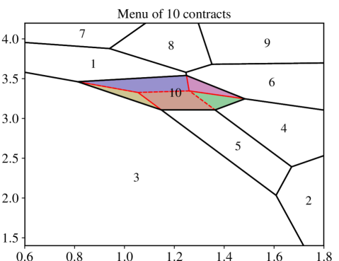
Figure 1: Evaluation of contract by dividing into subregions ($d=2$)
The green polyhedron corresponds to $F_{4,-10}\cap V_{10}$.

Algorithm 3a updateImpMetric   ($L_{1}$ error)

1:$I$, $(V_{i})_{i\in S}$, $(F_{j,-i})_{i\in I,j\in J_{i}}$

2:for $i\in I$ do$\triangleright$ Update metric on cells

3:    $\nu_{i}\leftarrow\sum_{j\in J_{i}}\iint_{F_{j,-i}\cap V_{i}}(\hat{u}_{i}(x)-\hat{u}_{j}(x))\textnormal{d}x$

4:end for

5:return $\nu$

Algorithm 3b updateImpMetric  ($J$-based error)

1:$I$, $(V_{i})_{i\in S}$, $(F_{j,-i})_{i\in I,j\in J_{i}}$

2:$M_{0}\leftarrow\sum_{i\in S}\iint_{V_{i}}M(x,\hat{q}_{i})\textnormal{d}x$

3:for $i\in S$ do$\triangleright$ Update metric on cells

4:    $\delta_{L}\leftarrow\displaystyle\sum_{j\in J_{i}}\iint_{F_{j,-i}\cap V_{i}}L(x,\hat{u}_{i}(x),\hat{q}_{i})-L(x,\hat{u}_{j}(x),\hat{q}_{j})\textnormal{d}x$

5:    $\delta_{M}\leftarrow\sum_{j\in J_{i}}\iint_{F_{j,-i}\cap V_{i}}M(x,\hat{q}_{j})-M(x,\hat{q}_{i})\textnormal{d}x$

6:    $\nu_{i}\leftarrow\delta_{L}-C(M_{0})+C(M_{0}+\delta_{M})$

7:end for

Proposition III.4 (Critical steps)

Let $m$ be the maximum number of neighbors of a polyhedral cell during the execution of the algorithm (for all $t$ and $i$, $|J_{i}|\leq m$). Then,

• The number of linear programs $(P^{S}_{i})$ solved in Algo. 1 is in $O(m|\Sigma|)$,

• The number of computations of a vertex representation of a polyhedral cell (calls to Vrep$(S,i)$ / reverse search) is in $O(m^{2}|\Sigma|)$.

By comparison with III.4, a naïve implementation (full recomputation of the importance metric at each step) of the two algorithms would respectively lead to a number of critical steps in $O(|\Sigma|^{2})$ and $O(m|\Sigma|^{2})$. Each linear program $P^{S}_{i}$ can be solved in polynomial time (by an interior point method). Reverse search has an incremental running time of $O(|\Sigma|d)$ per vertex if the input is nondegenerate, see [24].

IV APPLICATION TO ELECTRICITY MARKETS

IV-A Price elasticity

Let us consider a provider holding several contracts, each of them defined by a fixed price component $p\in\operatorname{\mathbb{R}}$ (in €), and $d$ variable price components $z\in\operatorname{\mathbb{R}}^{d}$ (in €/kWh). In France, the contracts often take into account $d=2$ time periods, with different prices for Peak / Off-peak consumptions. Moreover, the price coefficients $(p,z)$ of each contract are supposed to belong to a non-empty polytope $P\times Z\subset\operatorname{\mathbb{R}}^{d+1}$:

Assumption IV.1

Let $p^{-},p^{+}$ be in $\operatorname{\mathbb{R}}_{>0}$ and $z^{-},z^{+}$ be in $\operatorname{\mathbb{R}}^{d}_{>0}$. Then, $P=[p^{-},p^{+}]$, and the polytope $Z$ is of the following form:

$$Z:=\left\{z^{-}\leq z\leq z^{+}\mid z_{i_{1}}\leq\kappa_{i_{1},i_{2}}z_{i_{2}}\text{ for }i_{1}\leq_{\mathcal{P}}i_{2}\right\}\enspace,$$

where $\mathcal{P}$ is a partially ordered set (poset) of $\{1,\ldots,d\}$, and $\leq_{\mathcal{P}}$ the ordering relation, and $\kappa_{i_{1},i_{2}}>0$. When $\kappa\equiv 1$, $z^{-}\equiv 0$ and $z^{+}\equiv 1$, $Z$ is known as an order polytope [25].

IV.1 is natural for the electricity pricing problem: the price can be freely determined within a box (bounds), as long as some inequalities between peak price coefficients and off-peak price coefficients are fulfilled.

We suppose that each agent in the (infinite-size) population is characterized by a reference consumption vector $\check{x}\in X\subset\operatorname{\mathbb{R}}^{d}_{>0}$. Here, supposing a continuum of agents is justified since we consider in the application case the population of a whole country. We suppose that the consumption is elastic to prices, i.e., a consumer can deviate from its reference consumption $\check{x}$. In addition, we suppose that electricity elasticity can be captured into a utility-based framework, see e.g. [26] for the properties that the utility must satisfy. Here, we focus on isoelastic utilities:

Assumption IV.2 (Isoelastic utility function)

For a reference consumption $\check{x}$, the utility of consuming an amount of energy $x\in\operatorname{\mathbb{R}}^{d}_{\geq 0}$ is depicted through a Constant Relative Risk Aversion (CRRA,[27, 28]) or isoelastic utility:

$$\mathcal{U}_{\check{x}}:x\in\operatorname{\mathbb{R}}^{d}_{\geq 0}\mapsto\frac{1}{\eta}\sum_{i=1}^{d}\beta_{\check{x}i}(x_{i})^{\eta},\;\eta\in(\scalebox{0.5}[1.0]{$-$}\infty,0)\cup(0,1]\enspace.$$ (8)

The coefficient $\eta$ is called the risk aversion coefficient.

In this context, this elasticity measure depicts the easiness of a customer to adopt another energy source to fulfill his needs. In [28], the authors model the electric elasticity by this kind of utility function, and separate the case $\eta<0$ and $\eta\in(0,1]$. The first regime ($\eta<0$) will model a household consumption: the satisfaction coming from consuming energy saturates to a maximum utility, and a zero consumption is prohibited. In contrast, the second regime ($\eta\in(0,1]$) will represent the high flexibility of the industrial sector, which can adapt more easily its consumption according to price. We refer to [29] and references therein for empirical studies on the intensity of the elasticity coefficient $\eta$.

For a contract defined by price coefficients $(p,z)\in\operatorname{\mathbb{R}}\times\operatorname{\mathbb{R}}^{d}$, a consumer $\check{x}$ will optimize his consumption in order to maximize the welfare function, obtained by subtracting the electricity cost to (8):

$$\operatorname{\mathcal{U}}^{*}_{\check{x}}:(p,z)\in\operatorname{\mathbb{R}}\times\operatorname{\mathbb{R}}^{d}\mapsto\max_{x\in{\operatorname{\mathbb{R}}_{\geq 0}}^{d}}\left\{\operatorname{\mathcal{U}}_{\check{x}}(x)-\left<x,z\right>\right\}-p\enspace.$$ (9)

We denote by $\operatorname{\mathcal{U}}^{*}_{\check{x}}$ the welfare function as the maximization term in (9) corresponds to a Fenchel-Legendre transform up to a change of sign. As a consequence, $\operatorname{\mathcal{U}}^{*}_{\check{x}}$ is convex and nonincreasing. We now make the following assumption to fix the value of $\beta$:

Assumption IV.3

The reference consumption $\check{x}\in\operatorname{\mathbb{R}}^{d}$ is obtained for reference prices $\check{p}\in\operatorname{\mathbb{R}}$ and $\check{z}\in\operatorname{\mathbb{R}}^{d}$.

Under IV.3, the optimal consumption of customer $\check{x}$ on period $i\in\{1,\ldots,d\}$, denoted $\operatorname{\mathcal{E}}_{\check{x}i}$, is given by

$$\operatorname{\mathcal{E}}_{\check{x}i}(z)=\check{x}_{i}\left(z_{i}/\check{z}_{i}\right)^{\frac{-1}{1-\eta}}\;\geq 0\enspace,$$ (10)

and the welfare function is given by

$$\operatorname{\mathcal{U}}^{*}_{\check{x}}(p,z)=\left(\tfrac{1}{\eta}-1\right)\sum_{i=1}^{d}\check{x}_{h}\check{z}_{h}\left(z_{h}/\check{z}_{h}\right)^{\frac{-\eta}{1-\eta}}-p\enspace.$$ (11)

Equations 10 and 11 are obtained from the first order optimality condition (zero derivative) for (9) ($\beta_{\check{x}i}=\check{z}_{h}\left(\check{x}_{h}\right)^{1-\eta}$).

IV-B Infinite-size menu of offers

In this section, we relax the assumption of a finite number of contracts, by supposing that the provider is able to define as many offers as consumers. Therefore, the infinite-size menu of offers can be represented by two functions $p:X\to\operatorname{\mathbb{R}}$ and $z:X\to\operatorname{\mathbb{R}}^{d}$, representing respectively the fixed price component and the variable price components. Let us define the (weighted) invoice of a consumer as

$$\operatorname{\mathcal{L}}_{\check{x}}:(p,z)\in\operatorname{\mathbb{R}}\times\operatorname{\mathbb{R}}^{d}\mapsto(p+\left<\operatorname{\mathcal{E}}_{\check{x}}(z),z\right>)\rho(\check{x})\enspace,$$ (12)

where $\rho(\check{x})\geq 0$ represents the density of customers with reference consumption $\check{x}$. The provider’s revenue maximization problem is then

$$\max_{p,z} \;\operatorname{\mathcal{J}}^{1}(p,z)-\operatorname{\mathcal{J}}^{2}(z)$$ (13a)

s.t. $$\;\operatorname{\mathcal{U}}^{*}_{x}(p(x),z(x))\geq\operatorname{\mathcal{U}}^{*}_{x}(p(y),z(y)),\,\forall x,y\in X$$ (13b)

$$\;\operatorname{\mathcal{U}}^{*}_{x}(p(x),z(x))\geq R(x),\,\forall x\in X$$ (13c)

$$\;p(x)\in P,\;z(x)\in Z$$ (13d)

where $\operatorname{\mathcal{J}}^{1}(p,z)=\int_{X}\operatorname{\mathcal{L}}_{x}(p(x),z(x))\textnormal{d}x$ and $\operatorname{\mathcal{J}}^{2}(z)=C\left(\int_{X}\sum_{i=1}^{d}\operatorname{\mathcal{E}}_{xi}(z(x))\rho(x)\textnormal{d}x\right)$.

Equations 13b and 13c are respectively the incentive-compatibility condition and participation constraint. Taking $C$ as a strictly convex increasing function of the global consumption is often considered in the literature. In particular, this cost function is often modeled as a piecewise linear function, see e.g. [18], or as a quadratic function, see e.g. [17]. In fact, the marginal cost to supply electricity is not constant and increases with the consumption. The convexity of the reservation utility is also a classical assumption, as this reservation utility should be a supremum over the utilities of alternative offers (each of them being linear function of the reference consumption).

Let us make the following change of variables:

$$q_{i}:=(z_{i}/\check{z}_{i})^{\frac{-\eta}{1-\eta}}\enspace.$$

Then, the consumption on period $i\in\{1,\ldots,d\}$ is a convex function of $q_{i}$, expressed as $\mathfrak{E}_{\check{x}i}(q_{i})=\check{x}_{i}[q_{i}]^{\frac{1}{\eta}}\enspace,$ and both the utility and the weighted invoice now read as linear functions of $p$ and $q$: defining $\alpha=(\eta^{\scalebox{0.5}[1.0]{$-$}1}-1)\check{z}$,

$$u(x) :=\left<x,\alpha\odot q(x)\right>-p(x)\enspace,$$ (14)

$$L(x,u(x),q(x)) :=\left(\tfrac{1}{\eta}\left<x,\check{z}\odot q(x)\right>-u(x)\right)\rho(x)\enspace,$$

Theorem IV.1

Under IV.1, the provider’s revenue maximization problem (13) is equivalent to a monopolist problem of the form (4) with

$$M(x,q(x)):=\rho(x)\sum_{i=1}^{d}x_{i}[q_{i}(x)]^{\tfrac{1}{\eta}}$$ (15)

and, if $\eta<0$,

$$Q=\left\{q\in\operatorname{\mathbb{R}}^{d}\left|\begin{split}&\left(z^{-}/\check{z}\right)^{\frac{-\eta}{1-\eta}}\leq q\leq\left(z^{+}/\check{z}\right)^{\frac{-\eta}{1-\eta}}\\ &q_{i_{1}}\leq\left(\kappa_{i_{1},i_{2}}\tfrac{\check{z}_{i_{2}}}{\check{z}_{i_{1}}}\right)^{\frac{-\eta}{1-\eta}}q_{i_{2}}\text{ for }i_{1}\leq_{\mathcal{P}}i_{2}\end{split}\right.\right\},$$

otherwise,

$$Q=\left\{q\in\operatorname{\mathbb{R}}^{d}\left|\begin{split}&\left(z^{+}/\check{z}\right)^{\frac{-\eta}{1-\eta}}\leq q\leq\left(z^{-}/\check{z}\right)^{\frac{-\eta}{1-\eta}}\\ &q_{i_{1}}\geq\left(\kappa_{i_{1},i_{2}}\tfrac{\check{z}_{i_{2}}}{\check{z}_{i_{1}}}\right)^{\frac{-\eta}{1-\eta}}q_{i_{2}}\text{ for }i_{1}\leq_{\mathcal{P}}i_{2}\end{split}\right.\right\}$$

Proof:

Owing to assumption on the set $Q$ and the strict monotonicity of $z\mapsto z^{\frac{-\eta}{1-\eta}}$ (increasing for $\eta<0$ and decreasing for $\eta>0$), one can explicitly derive the form of $Q$. The rest of the formulation is immediate. ∎

V NUMERICAL RESULTS

V-A Instance

The numerical results were obtained on a laptop i7- 1065G7 CPU@1.30GHz. We provide in Table I the values of the parameters used in the application. In particular, we consider reference prices $(\hat{p},\hat{z})$ corresponding to French regulated prices, and reference consumption spread around the mean French consumption per household ($\operatorname{\mathcal{E}}_{\text{moy}}=4$MWh). The cost function is taken as a quadratic function, scaled so that the marginal cost $C^{\prime}(\operatorname{\mathcal{E}}_{\text{moy}})=0.08$€/kWh. In comparison, the production cost is estimated in France around 0.05€/kWh for nuclear plants and up to 0.09€/kWh for wind energy.

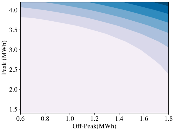
(a) Infinite-size menu

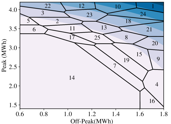
(b) Menu of 25 contracts

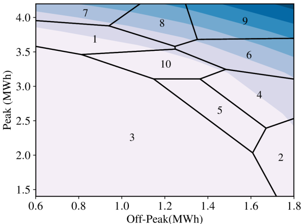
(c) Menu of 10 contracts

Figure 2: $L_{1}$-norm pruning for the electricity market case.
The normalized utility $u-R$ is depicted with colormap (light gray corresponds to the zero value and blue to high value).

$\eta$	-0.1
$\check{p}$	140€
$\check{z}$	(0,174,019)€/kWh
$C(\cdot)$	$0.01(\cdot)^{2}$
$(p^{-},p^{+})$	$(0,500)$€
$(q_{1}^{-},q_{1}^{+})$	$(0.05,0.5)$€/kWh
$(q_{2}^{-},q_{2}^{+})$	$(0.05,0.5)$€/kWh
$\rho$	Uniform$([0.6,1.8]\times[1.4,4.2])$
$R(\cdot)$	linear function (one regulated contract)

TABLE I: Instance used in the numerical results.

We display in Figure 2 the infinite-size menu and the quantized solution for two different sizes of menu (25 contracts and 10 contracts). In each cell $\operatorname{\mathcal{C}}_{i}$, the contract $i$ brings to customers of reference consumption $x\in\operatorname{\mathcal{C}}_{i}$ the maximal utility given the quantized menu, i.e., $\hat{u}_{S}(x)=\hat{u}_{i}(x)$ for $x\in\operatorname{\mathcal{C}}_{i}$. We observe that there is a region/cell (light gray region) where the monopolist reproduces the alternative option (of utility $R$). On the other side, for high consumption (peak or off-peak), the monopolist manages to design contracts that provide strictly higher utility than the regulated offer, and at the same time, procure to the monopolist a higher revenue.

V-B Comparison of pruning objectives

In the upper graph of Figure 3, the three pruning objectives studied in the paper ($L_{\infty}$, $L_{1}$ and $J$-based) are compared with the 1-step approach of [13, 14]. The approach consists in sorting the importance metrics for all $i\in\Sigma$, and directly taking the $n$ contracts with highest importance metric (here we consider the $J$-based importance metric). We display the relative objective loss, defined as 1 - $J_{t}/J_{\text{ref}}$, where $J_{t}$ is the objective for a menu of size $t$ and $J_{\text{ref}}$ the objective obtained with the infinite-size menu. Note that removing a contract can induce a violation of the full-participation constraint ($u\geq R$). Therefore, in order to recover a feasible solution at each iteration, we lift up the solution with the simple rule $u\leftarrow u+\max\{\max_{x\in X}\{R(x)-u(x)\},0\}$.

On this example, the pruning procedure of Algo. 2 (greedy descent) leads to a significant loss reduction, whatever the criterion, compared with the 1-step approach. As expected, we observe that the $J$-based pruning has the smallest relative loss in the objective, as we minimize the error at each iteration of the process. In contrast, the $L_{\infty}$-norm does not capture sufficiently well the behavior of the objective function $J$, and has larger objective loss, even for a large number of contracts.

We also depicted the cumulated time along the iterations in the lower graph of Figure 3 (we do not display the time for the 1-step procedure, as it is very fast, in less than 0.5s). For comparison, we add the cumulative time of a “naïve” $J$-based pruning, recomputing at each iteration the importance metric of each cell (global update). On this example, we observe that the computational time is already reduced by a factor almost 3 (this factor would be greater in higher dimension, as the neighborhood would be larger). As expected, the $L_{\infty}$ criterion is the fastest, owing to the fast local update rule exploiting the sparsity of optimal Lagrange multipliers (Algorithm 1), and the $J$-based and $L_{1}$-norm criteria have similar computational time, as they use the same algorithmic architecture, see Algo. 2. In terms of loss minimization, the $J$-based pruning shows a loss of revenue reduced by a factor of around $2$ by comparison with other methods. This approach allows us to determine the minimum number of contracts given an admissible revenue loss: e.g., Figure 3 shows that, with a $J$-based quantization, a menu of $10$ contracts suffices to limit the revenue loss to $4$%.

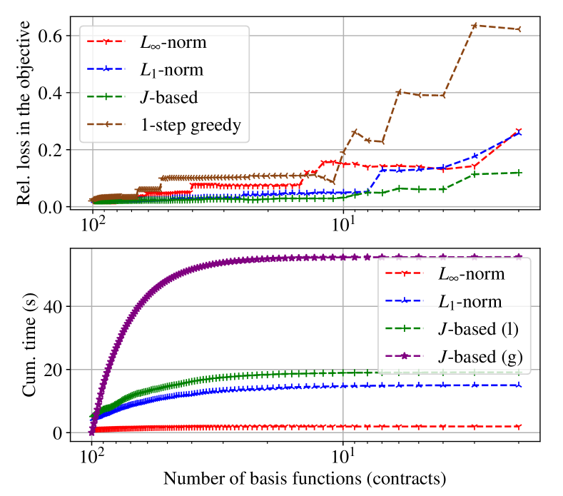
Figure 3: Comparison of error bounds for the three types of pruning objective. The upper graph shows the loss of optimality induced by a reduced number of contracts. The lower graph depicts cumulative time along the iterations. (g) stands for global update while (l) stands for local update.

VI CONCLUSION

We have addressed a nonlinear pricing problem incorporating coupling costs. This arises in electricity markets, where supply costs depend on the global consumption. We have developed a quantization procedure, allowing to maximize the revenue of a provider, given a cardinality constraint on the set of contracts. This relies on refined pruning procedures, inspired by the max-plus basis methods in numerical optimal control. In particular, we exploited the local nature of the pruning process, in order to reduce the computational time. Thus, this leads to a new class of applications for methods originally developed in optimal control, and this also improves the complexity of a key ingredient of these methods.

A strong parallel with vector quantization can be made, see e.g. [30]. In this context, a different quantization problem is addressed by Lloyd’s procedures, ibid.. Whether these ideas can be adapted to the quantization of the maximum of affine functions with revenue criterion is left for further work.

VII APPENDIX

VII-A Proof of Theorem II.2

Using II.1, for any solution, $\nabla u(x)=\alpha\odot q(x)$ for a.e. $x\in X$. We then directly study the existence and uniqueness in $(u,\nabla u)$.

Existence. Let $H^{1}(X)$ be the Sobolev space associated with $X$. We define

$$\operatorname{\mathcal{K}}=\left\{u\left|\begin{split}&u\text{ convex and }u\geq R\\ &u(x)\in U_{x},\;\alpha^{\scalebox{0.5}[1.0]{$-$}1}\odot\nabla u(x)\in Q\;,\;\forall x\in X\end{split}\right.\right\}\enspace.$$

The set $\operatorname{\mathcal{K}}$ is a closed, convex and bounded subset of $H^{1}(X)$ (it is bounded since $X$ is bounded and $\|u\|_{L_{\infty}}$ and $\|\nabla u\|_{L_{\infty}}$ are bounded too; it is convex since $R$ is convex).

Besides, $J$ is concave (II.1). Moreover, as $Q\subset\operatorname{\mathbb{R}}_{>0}^{d}$, there exist $a,b>0$ such that for any $x\in X$, $a\leq\|\nabla u(x)\|\leq b$. Therefore, there exists $c\in\operatorname{\mathbb{R}}_{+}$ such that $|J(u,\nabla u)|\leq c$, and as a consequence, $J$ is continuous on $\operatorname{\mathcal{K}}$, see [31, Chapter 1, Proposition 2.5].

Using the fact that $H^{1}(X)$ is reflexive and [31, Chapter 2, Proposition 1.2], Problem (4) admits at least one solution.

Uniqueness. (Same arguments as in [4]) Let now consider two distinct solutions $u_{1}$ and $u_{2}$. Then, if $\nabla u_{1}\neq\nabla u_{2}$ on a measurable subset, any function $tu_{1}+(1-t)u_{2}$ is valid and gives a strictly better solution than $u_{1}$ and $u_{2}$ (due to strict convexity of the cost function $u\mapsto C(\int_{X}M(x,\nabla u(x))\textnormal{d}x)$ and linearity of $L$). Therefore, $u_{1}-u_{2}$ is a constant function. By linearity of $L$, the objective value obtained with $u_{1}$ and $u_{2}$ differ by the same constant. This contradicts the optimality of the two solutions $u_{1}$ and $u_{2}$.

VII-B Fast metric updates using Green’s formula

The next proposition allows us to implement efficiently the local updates of the importance metric performed in 3a–3b.

Proposition VII.1

Let $P$ a 2D-polytope describes by its vertices $(x_{i},y_{i})\in\operatorname{\mathbb{R}}^{2}$ (counter-clockwise ordered). Then for any $a,b,c\in\operatorname{\mathbb{R}}$,

$$\iint_{P}(ax+by+c)dxdy=\sum_{i=1}^{N}\left[\begin{split}&\oint_{y_{i}}^{y_{i+1}}b(q_{i}+\tfrac{1}{\tau_{i}}y)ydy\\ &\scalebox{0.5}[1.0]{$-$}\oint_{x_{i}}^{x_{i+1}}(ax+c)(p_{i}+\tau_{i}x)dx\end{split}\right],$$

with $\tau_{i}=\frac{y_{i+1}-y_{i}}{x_{i+1}-x_{i}}$, $p_{i}:=y_{i}-\tau_{i}x_{i}$ and $q_{i}:=x_{i}-\frac{1}{\tau}y_{i}$.

Proof:

The application of the Green formula gives :

$$\iint_{P}(ax+by+c)dxdy=\oint_{\operatorname{\mathcal{C}}_{P}}(bxy)dy-(ax+c)ydx\enspace,$$

where $\operatorname{\mathcal{C}}_{P}$ is the contour of the polytope $P$. We then decompose on each edges, and use the change of variable $x=q+y/\tau$ in the first integral and $y=x+\tau x$ in the second one. ∎

References

- [1] John Scott “Rational choice theory” In Understanding contemporary society: Theories of the present 129, 2000, pp. 126–138
- [2] M. Simaan and J.. Cruz “On the Stackelberg strategy in nonzero-sum games” In Journal of Optimization Theory and Applications 11.5 Springer ScienceBusiness Media LLC, 1973, pp. 533–555 DOI: 10.1007/bf00935665
- [3] Tilman Börgers, Daniel Krähmer and Roland Strausz “An Introduction to the Theory of Mechanism Design” Oxford University PressNew York, 2015 DOI: 10.1093/acprof:oso/9780199734023.001.0001
- [4] Jean-Charles Rochet and Philippe Choné “Ironing, sweeping, and multidimensional screening” In Econometrica JSTOR, 1998, pp. 783–826
- [5] Michael Mussa and Sherwin Rosen “Monopoly and product quality” In Journal of Economic theory 18.2 Academic Press, 1978, pp. 301–317
- [6] Mark Armstrong “Multiproduct Nonlinear Pricing” In Econometrica 64.1 JSTOR, 1996, pp. 51 DOI: 10.2307/2171924
- [7] Guillaume Carlier and Xavier Dupuis “An iterated projection approach to variational problems under generalized convexity constraints” In Applied Mathematics and Optimization 76.3 Springer, 2017, pp. 565–592
- [8] Jean-Marie Mirebeau “Adaptive, anisotropic and hierarchical cones of discrete convex functions” In Numerische Mathematik 132.4 Springer, 2016, pp. 807–853
- [9] Dirk Bergemann, Edmund Yeh and Jinkun Zhang “Nonlinear pricing with finite information” In Games and Economic Behavior 130 Elsevier BV, 2021, pp. 62–84 DOI: 10.1016/j.geb.2021.08.004
- [10] Martine Labbé, Patrice Marcotte and Gilles Savard “A bilevel model of taxation and its application to optimal highway pricing” In Management science 44 INFORMS, 1998, pp. 1608–1622
- [11] Elizabeth Baldwin and Paul Klemperer “Understanding Preferences: “Demand Types”, and the Existence of Equilibrium With Indivisibilities” In Econometrica 87.3 The Econometric Society, 2019, pp. 867–932 DOI: 10.3982/ecta13693
- [12] William M. McEneaney “A Curse-of-Dimensionality-Free Numerical Method for Solution of Certain HJB PDEs” In SIAM Journal on Control and Optimization 46.4 Society for Industrial & Applied Mathematics (SIAM), 2007 DOI: 10.1137/040610830
- [13] William M. McEneaney, Ameet Deshpande and Stephane Gaubert “Curse-of-complexity attenuation in the curse-of-dimensionality-free method for HJB PDEs” In 2008 American Control Conference IEEE, 2008 DOI: 10.1109/acc.2008.4587234
- [14] Stephane Gaubert, William McEneaney and Zheng Qu “Curse of dimensionality reduction in max-plus based approximation methods: Theoretical estimates and improved pruning algorithms” In IEEE Conference on Decision and Control and European Control Conference IEEE, 2011 DOI: 10.1109/cdc.2011.6161386
- [15] Stephane Gaubert, Zheng Qu and Srinivas Sridharan “Bundle-based pruning in the max-plus curse of dimensionality free method” In Proceedings of the 21st International Symposium on Mathematical Theory of Networks and Systems July 7-11, 2014. Groningen, The Netherland, 2014, pp. 166–172
- [16] W.. McEneaney and P.. Dower “The Principle of Least Action and Fundamental Solutions of Mass-Spring and N-Body Two-Point Boundary Value Problems” In SIAM Journal on Control and Optimization 53.5, 2015 DOI: 10.1137/130921908
- [17] W. Ackooij, I. Lopez, A. Frangioni, F. Lacalandra and M. Tahanan “Large-scale unit commitment under uncertainty: an updated literature survey” In Annals of Operations Research 271.1 Springer ScienceBusiness Media LLC, 2018, pp. 11–85 DOI: 10.1007/s10479-018-3003-z
- [18] Ekaterina Alekseeva, Luce Brotcorne, Sébastien Lepaul and A. Montmeat “A bilevel approach to optimize electricity prices” In Yugoslav Journal of Operations Research, 2019
- [19] Ivar Ekeland and Santiago Moreno-Bromberg “An algorithm for computing solutions of variational problems with global convexity constraints” In Numerische Mathematik 115.1 Springer ScienceBusiness Media LLC, 2009, pp. 45–69 DOI: 10.1007/s00211-009-0270-2
- [20] Jean-Charles Rochet “A necessary and sufficient condition for rationalizability in a quasi-linear context” In Journal of Mathematical Economics 16.2 Elsevier BV, 1987, pp. 191–200 DOI: 10.1016/0304-4068(87)90007-3
- [21] Guillaume Carlier “A general existence result for the principal-agent problem with adverse selection” In Journal of Mathematical Economics 35.1 Elsevier BV, 2001, pp. 129–150 DOI: 10.1016/s0304-4068(00)00057-4
- [22] Marianne Akian, Stéphane Gaubert and Asma Lakhoua “The Max-Plus Finite Element Method for Solving Deterministic Optimal Control Problems: Basic Properties and Convergence Analysis” In SIAM Journal on Control and Optimization 47.2 Society for Industrial & Applied Mathematics (SIAM), 2008, pp. 817–848 DOI: 10.1137/060655286
- [23] Steven Fortune “Voronoi Diagrams and Delaunay Triangulations” In Lecture Notes Series on Computing World Scientific, 1995, pp. 225–265 DOI: 10.1142/9789812831699˙0007
- [24] David Avis “A Revised Implementation of the Reverse Search Vertex Enumeration Algorithm” In Polytopes — Combinatorics and Computation Basel: Birkhäuser Basel, 2000, pp. 177–198 DOI: 10.1007/978-3-0348-8438-9˙9
- [25] Richard P. Stanley “Two poset polytopes” In Discrete & Computational Geometry 1.1 Springer ScienceBusiness Media LLC, 1986, pp. 9–23 DOI: 10.1007/bf02187680
- [26] Pedram Samadi, Hamed Mohsenian-Rad, Robert Schober and Vincent W.. Wong “Advanced Demand Side Management for the Future Smart Grid Using Mechanism Design” In IEEE Transactions on Smart Grid 3.3, 2012, pp. 1170–1180 DOI: 10.1109/TSG.2012.2203341
- [27] Robert S. Pindyck “Uncertain outcomes and climate change policy” In Journal of Environmental Economics and Management 63.3 Elsevier BV, 2012, pp. 289–303 DOI: 10.1016/j.jeem.2011.12.001
- [28] Clémence Alasseur, Ivar Ekeland, Romuald Élie, Nicolás Hernández Santibáñez and Dylan Possamaï “An Adverse Selection Approach to Power Pricing” In SIAM Journal on Control and Optimization 58.2 Society for Industrial & Applied Mathematics (SIAM), 2020, pp. 686–713 DOI: 10.1137/19m1260578
- [29] Amir Niromandfam and Saeid Pashaei Choboghloo “Modeling electricity demand, welfare function and elasticity of electricity demand based on the customers risk aversion behavior” arXiv, 2020 DOI: 10.48550/ARXIV.2010.07600
- [30] Gilles Pagès “Introduction to vector quantization and its applications for numerics” In ESAIM: Proceedings and Surveys 48 EDP Sciences, 2015, pp. 29–79 DOI: 10.1051/proc/201448002
- [31] Ivar Ekeland and Roger Temam “Convex analysis and variational problems” SIAM, 1999