$B\to X_{u}\ell\nu_{\ell}\gamma$ and determination of non-perturbative parameters

Abstract

This article explores the calculation of non-perturbative parameters present in the matrix element of semileptonic inclusive $B$ decay. These are important for inclusive determination of the Cabbibo-Kobayashi-Maskawa (CKM) parameters in the standard model. We focus on calculating the rate for radiative inclusive decay, $B\to X_{u}\ell\nu_{\ell}\gamma$, where $\gamma$ is hard. By comparing both the radiative and non-radiative ($B\to X_{u}\ell\nu_{\ell}$) modes are found to require the same non-perturbative parameters. We propose forming ratios, $R_{1}$ and $R_{2}$, from $B\to X_{u}\ell\nu_{\ell}\gamma$ and $B\to X_{u}\ell\nu_{\ell}$ widths in different lepton energy ranges respectively. Our results provide an efficient way to unambiguously calculate the non-perturbative parameters, especially when combined with total width calculations of $B\to X_{u}\ell\nu_{\ell}$. This is in heavy quark expansion shown explicitly by working to $\mathcal{O}(\frac{1}{m_{b}})$ and determining $\lambda_{1}$ and $\lambda_{2}$.

1 Introduction

$B$ meson decays are complex processes that provide an ideal platform for precision studies of the Standard Model (SM) as they involve various physical scales. Inclusive decay modes (the final state mesons are summed over) are considered to be theoretically cleaner than exclusive ones (final state particles are explicitly identified) as the latter involve transition form factors which are rather difficult to evaluate. The inclusive $B$ meson decays are theoretically cleaner as they take the advantage of hard scale, $m_{b}$, which is much larger than $\Lambda_{QCD}$. The presence of the hard scale enables the use of the Heavy Quark Expansion (HQE) [1, 2] and local Operator Product Expansion (OPE) [3, 4], and hence a systematic theoretical treatment of the decay rates.

The HQE is a fundamental tool in the study of heavy quark physics. It provides a series expansion in $\frac{1}{m_{Q}}$, where $Q$ is the heavy quark[5]. Though the mass of $b$ quark is heavy enough to use the expansion in $\frac{1}{m_{b}}$, yet corrections to the heavy quark limit are significant for achieving high precision. OPE is a powerful tool that enables a systematic treatment of non-perturbative Quantum Chromodynamics (QCD) effects by seperating the effects originating at large and small distances [6, 7]. For a heavy quark system, it turns out to be a series expansion in powers of $\frac{\Lambda_{\text{QCD}}}{m_{b}}$ [8, 9] when combined with the theory of heavy quark expansion.

The corrections to the leading term ($m_{b}\to\infty$) in the heavy quark expansion are expected to be small in end region of the phase space. This part of the phase space allows the contribution of several hadronic states which satisfy the condition: $m_{X}^{2}\to m_{q}^{2}+\#\Lambda_{\text{QCD}}m_{b}$. The observables, like the decay rate, which average over these hadronic states can then be predicted reliably. To $\mathcal{O}(\frac{1}{m_{b}})$ in HQE, the major uncertainty in these predictions arises from the values of non-perturbative parameters, $\lambda_{1}$ and $\lambda_{2}$. Throughout the article, we consistently work to $\mathcal{O}(\frac{1}{m_{b}})$ in HQE. These parameters are defined as [10, 11]

$$\lambda_{1}=\frac{1}{2m_{H_{Q}}}\langle H_{Q}|\bar{Q}{\bf\Pi}^{2}Q|H_{Q}\rangle,\hskip 14.22636pt({\bf\Pi}=i{\bf D})\hskip 28.45274pt\text{and}\hskip 28.45274pt3\lambda_{2}=\frac{1}{2m_{H_{Q}}}\langle H_{Q}|\bar{Q}\frac{i}{2}\sigma_{\mu\nu}G^{\mu\nu}Q|H_{Q}\rangle$$ (1)

where, $D$ is covariant derivative, and $|H_{Q}\rangle$ represent the states of hadrons containing one heavy quark and light cloud (for $b$ hadrons $H_{Q}=B,\lambda_{b}$, etc.). The notation $\mu_{\pi}^{2}$ and $\mu_{G}^{2}$ is also used instead of $\lambda_{1}$ and $\lambda_{2}$ for $b$ hadrons. The two are related as [12]

$$\mu_{\pi}^{2}(B)=-\lambda_{1}+\mathcal{O}(\alpha_{s})\,\hskip 28.45274pt\text{and}\hskip 28.45274pt\mu_{G}^{2}(B)=3\lambda_{2}$$ (2)

Physically, $\lambda_{1}$ provides information about the average spatial momentum squared of the heavy quark, while $\lambda_{2}$ represents the amount of color magnetic field produced by the light cloud at the position of the heavy quark [13, 12].

In the past, the parameters $\lambda_{1}$ and $\lambda_{2}$ have been determined using QCD models [14, 15, 16, 17], and also have been extracted by fitting to the experimental data [18, 19, 20, 21, 22]. Ref. [23] determines $\mu_{\pi}^{2}$ and $\mu_{G}^{2}$ in quenched lattice QCD using the NRQCD action including $\mathcal{O}(\frac{1}{m_{Q}})$ for the heavy quark. They compute $\lambda_{2}$ explicitly but not $\lambda_{1}$, and rather calculate difference of matrix elements, using two different methods. Also, these two different methods of computation have followed different central values. Consequently, having an unambiguous predictions for these parameters becomes important.

In this article, we discuss how the experimental determination of the total decay width for $B\to X_{u}\ell\nu_{\ell}\gamma$ decay along with the data on the total decay width for $B\to X_{u}\ell\nu_{\ell}$ can help us in this regard. The emitted photon is a hard photon and the process should not be thought of as soft photon correction to $B\to X_{u}\ell\nu_{\ell}$. To this order in $\frac{1}{m_{b}}$, the decay widths of both these modes, i.e. $B\to X_{u}\ell\nu_{\ell}$ and $B\to X_{u}\ell\nu_{\ell}\gamma$, have linear dependence on $\lambda_{1}$ and $\lambda_{2}$:

$$\text{decay width}\sim A+B\lambda_{1}+C\lambda_{2}.$$ (3)

for different values of ${A,B,C}$ for the two modes. Therefore knowing (or experimentally measuring) one of the sides of these equations will provide a simultaneous set of linear equations which can then be solved to get unambiguous determinations of $\lambda_{1}$ and $\lambda_{2}$. While we are including terms $\mathcal{O}(\frac{1}{m_{b}})$ in HQE, it is straight forward to include higher order terms. To avoid the uncertainties which may arise due to the presence of the Cabibbo-Kobayashi-Maskawa (CKM) element ($V_{ub}$), we propose to consider the ratio of the decay width in different ranges of the leptonic energy instead of directly working with the decay width (see Section-4 for details). Such ratios are defined as

$$R_{1}=\frac{\int_{0}^{0.2}dy\frac{d\Gamma_{\gamma}}{dy}}{\int_{0}^{0.5}dy\frac{d\Gamma_{\gamma}}{dy}}\ \ \ \ \ \text{ and}\hskip 56.9055ptR_{2}=\frac{\int_{0}^{0.5}dy\frac{d\Gamma}{dy}}{\int_{0}^{1}dy\frac{d\Gamma}{dy}}$$ (4)

where $y$ is the lepton energy expressed in dimensionless units. The rest of the article is organised as follows: in Section- 2, as a warm up, we first calculate the decay width for the non-radiative process $B\to X_{u}\ell\nu_{\ell}$ mode. This is achieved by directly using the Cutkosky method applied to the amplitude in contrast with the usual approach of writing down the hadronic tensor in terms of invariant quantities and employing analytical properties. Both the approaches are actually equivalent and we explicitly verify that the result matches with [4, 11] as it should. In Section- 3, we provide the details of the calculation of the decay width for $B\to X_{u}\ell\nu_{\ell}\gamma$ mode. In Section- 4, we discuss our results for the differential decay rate for $B\to X_{u}\ell\nu_{\ell}\gamma$ and its sensitivity to the energy of the hard photon. Also, we provide a method to calculate (or determine) non-perturbative parameters $\lambda_{1}$ and $\lambda_{2}$. Finally, we conclude in Section-5 and discuss the implications of the decay rate of $B\to X_{u}\ell\nu_{\ell}\gamma$ for calculation of $\lambda_{1}$ and $\lambda_{2}$.

2 Decay rate of $B\to X_{u}\ell\nu_{\ell}$

The weak Hamiltonian density for the inclusive semi-leptonic $B$ meson decays to final state containing a $u$ quark ($B\to X_{u}\ell\nu_{\ell}$) is given by

$$\mathcal{H}_{weak}=\frac{4G_{F}}{\sqrt{2}}V_{ub}(\bar{u}\gamma_{\mu}P_{L}b)(\bar{\ell}\gamma^{\mu}P_{L}\nu_{\ell})$$ (5)

where, $G_{F}$ and $V_{ub}$ are Fermi constant and CKM element, respectively.

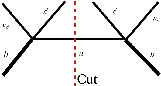
Figure 1: Representative Diagram of forward scattering for $b\to u\ell\nu_{\ell}$

The process of $B\to X_{u}\ell\nu_{\ell}$ involves the $b\to u$ transition and sum over the final state mesons containing the $u$ quark. To calculate the decay width for the inclusive process, the forward scattering matrix element is a useful quantity. Fig.(1) shows the Feynman diagram for the forward scattering matrix element of the inclusive semi-leptonic $B\to X_{u}\ell\nu_{\ell}$ decay. The imaginary part of the forward scattering matrix element or called the transition matrix element, $\langle B|\hat{T}|B\rangle$, is related to the decay to an inclusive final state through the optical theorem. It is given by

$$\Gamma\propto\frac{1}{2m_{B}}Im\big{\{}\langle B|\hat{T}(b\to u\to b)|B\rangle\big{\}}$$ (6)

where the operator sandwiched between the hadronic states is called forward scattering operator (or transition operator). The explicit form of the transition operator reads

$$\hat{T}^{\mu\nu}(b\to u\to b)=i\int d^{4}xe^{-iq.x}\frac{1}{2m_{B}}T\{J^{\mu\dagger}_{w}(x)J^{\nu}_{w}(0)\}$$ (7)

where $T$ denotes the time ordered product and $J^{\mu}_{w}\ (=\bar{u}\gamma^{\mu}P_{L}b)$ is the weak current. Further, the differential decay rate for $B\to X_{u}\ell\nu_{\ell}$ process is given by

$$\frac{d^{3}\Gamma}{dq^{2}dE_{\ell}dE_{\nu}} = \frac{1}{4}\sum_{X_{u}}\sum_{\text{spins}}\frac{1}{2m_{B}}|\langle X_{u}\ell\nu|\mathcal{H}_{weak}|B\rangle|^{2}\delta^{4}(p_{B}-p_{X}-p_{\ell}-p_{\nu})$$ (8)

$$= 2G_{F}^{2}|V_{ub}|^{2}\mathcal{M}_{\mu\nu}\mathcal{L}^{\mu\nu}$$

where $q^{2}=(p_{\ell}+p_{\nu})^{2}$, $E_{\ell}$ is the lepton energy, and $E_{\nu}$ is the neutrino energy. Furthermore, the leptonic tensor ($\mathcal{L}_{\mu\nu}$) is defined directly from the electroweak Lagrangian

$$\mathcal{L}_{\mu\nu}=(\bar{\nu}_{\ell}\gamma_{\mu}(1-\gamma_{5})\ell)(\bar{\ell}\gamma_{\nu}(1-\gamma_{5})\nu)$$ (9)

whereas, the hadronic tensor, $\mathcal{M}_{\mu\nu}$, is expressed in terms of matrix elements of electroweak currents, and is given by

$$\mathcal{M}_{\mu\nu}=\frac{1}{2m_{B}}\sum_{X_{u}}\langle B|J^{\mu}|X_{u}\rangle\langle|X_{u}|J^{\nu}|B\rangle\delta^{4}(p_{B}-p_{X}-p_{\ell}-p_{\nu}).$$ (10)

The hadronic tensor ($\mathcal{M}_{\mu\nu}$) is defined as the absorptive part of the matrix element of the transition operator (i.e. Eqn. (7)). Explicitly,

$$\mathcal{M}_{\mu\nu}=-i\hskip 2.84544ptDisc.(\langle B|\hat{T}_{\mu\nu}|B\rangle)$$ (11)

Instead of using the general parametrization for the hadronic tensor and relying on the analytical properties, we directly evaluate the transition operator ($\hat{T}_{\mu\nu}$) along with the leptonic tensor ($\mathcal{L}_{\mu\nu}$) to obtain the matrix element involved in the inclusive semi-leptonic $B\to X_{u}\ell\nu_{\ell}$ decay. At the lowest order in perturbation theory (i.e. in $\alpha_{s}$ expansion), the quark level amplitude ($\mathcal{M}_{NR}$) for the Fig. (1)) is given by

$$\mathcal{M}_{NR}=\frac{i}{(p_{b}+\Pi-q)^{2}-m_{u}^{2}}\bar{b}\gamma_{\nu}P_{L}(\not{p_{b}}+\not{\Pi}-\not{q}+m_{b})\gamma_{\mu}P_{L}b\mathcal{L}^{\mu\nu}$$ (12)

The subscript ‘NR’ refers to non-radiative process i.e. the process without a photon in the final state. Further, $p_{b}+\Pi$ is the effective momentum of $b$ quark, where $p_{b}=m_{b}v$ is heavy quark momentum while $\Pi$ is residual momentum of heavy quark. Also, $q\ (=p_{\ell}+p_{\nu})\sim\mathcal{O}(m_{b})$ while $\Pi$ $\sim\mathcal{O}(\Lambda_{\text{QCD}})$. Hence, the expansion of $\mathcal{M}_{NR}$ in powers of $\Pi$ produces an expansion in powers of $\frac{\Lambda_{\text{QCD}}}{m_{b}}$. Expanding the denominator to $(\frac{\Lambda_{\text{QCD}}}{m_{b}})^{2}$,

$$\frac{1}{(p_{b}+\Pi-q)^{2}-m_{u}^{2}} = \frac{1}{((p_{b}-q)^{2}-m_{u}^{2})}\Big{[}1-\frac{2(p_{b}-q).\Pi+\Pi^{2}}{((p_{b}-q)^{2}-m_{u}^{2})}+\frac{2((p_{b}-\Pi).\Pi)^{2}}{((p_{b}-q)^{2}-m_{u}^{2}))^{2}}\Big{]}$$ (13)

The hadronic part of $\mathcal{M}_{NR}$ is then sandwiched between the $B$ meson states. The obtained matrix elements are simplified as [11]

$$\langle B(v)|\bar{b}\gamma^{\mu}b|B(v)\rangle = 2p_{B}^{\mu}$$

$$\langle B(v)|\bar{b}\gamma_{\mu}\Pi_{\tau}b|B(v)\rangle = \frac{\lambda_{1}+3\lambda_{2}}{3m_{b}}(2g_{\mu\tau}-5v_{\mu}v_{\tau})$$

$$\langle B(v)|\bar{b}\gamma_{\mu}\Pi_{(\alpha}\Pi_{\beta)}b|B(v)\rangle = \frac{2\lambda_{1}}{3m_{b}}(g_{\alpha\beta}-v_{\alpha}v_{\beta})v_{\mu}$$

$$\langle B(v)|\bar{b}\gamma_{\mu}\Pi^{2}b|B(v)\rangle = \frac{2\lambda_{1}}{m_{b}}v_{\mu}$$ (14)

Next, we calculate the imaginary part of the denominator,

$$\frac{1}{((p_{b}-q)^{2}-m_{u}^{2})}\to(-2\pi i)\delta((p_{b}-q)^{2}-m_{u}^{2})\Theta((p_{b}^{0}-q^{0})).$$ (15)

Integrating over the neutrino energy, the double differential decay rate for $B\to X_{u}\ell\nu_{\ell}$ mode is calculated as

$$\frac{d^{2}\Gamma}{dyd\hat{q^{2}}} = \frac{G_{F}^{2}|V_{ub}|^{2}m_{b}^{5}}{96\pi^{3}}y\Big{[}6(1-\frac{\hat{q^{2}}}{y})(1-\rho-y+\hat{q^{2}})+\lambda_{1}\Big{(}-3+3\rho+4\frac{\hat{q}^{2}}{y}-4\rho\frac{\hat{q^{2}}}{y}-6\hat{q^{2}}+4\frac{(\hat{q^{2}})^{2}}{y}$$ (16)

$$- \delta(z)\Big{(}1-2\rho+\rho^{2}-3y(1-\rho)-3\frac{\hat{q^{2}}}{y}+2\rho\frac{\hat{q^{2}}}{y}+\rho^{2}\frac{\hat{q^{2}}}{y}+11\hat{q^{2}}-3\rho\bar{q^{2}}-3x\hat{q^{2}}-6\frac{(\hat{q^{2}})^{2}}{y}-2\rho\frac{(\hat{q^{2}})^{2}}{y}+2(\hat{q^{2}})^{2}$$

$$+ \frac{(\hat{q^{2}})^{3}}{y}\Big{)}+\delta^{\prime}(z)(1-\frac{\hat{q^{2}}}{y})(1-\rho-y+\hat{q^{2}})(1-2\rho+\rho^{2}-2\hat{q^{2}}-2\rho\hat{q^{2}}+(\hat{q^{2}})^{2})\Big{)}+3\lambda_{2}\Big{(}1-5\rho+2\frac{\hat{q^{2}}}{y}$$

$$+ 10\rho\frac{\hat{q^{2}}}{y}+10\hat{q^{2}}(1-\frac{\hat{q^{2}}}{y})-\delta(z)\Big{(}-1+6\rho-5\rho^{2}+y(1-5\rho)+\frac{\hat{q^{2}}}{y}(1-2\rho)+5\rho^{2}\frac{\hat{q^{2}}}{y}+\hat{q^{2}}(1+15\rho)$$

$$+ 5y\hat{q^{2}}-2\frac{(\hat{q^{2}})^{2}}{y}-10(1+y)\frac{(\hat{q^{2}})^{2}}{y}+\frac{(\hat{q^{2}})^{3}}{y}\Big{)}\Big{)}\Big{]}$$

where $y=\dfrac{2E_{\ell}}{m_{b}}$, $q^{2}=(p_{\ell}+p_{\nu})^{2}$, $\hat{q^{2}}=\dfrac{q^{2}}{m_{b}^{2}}$, $\rho=\dfrac{m_{u}^{2}}{m_{b}^{2}}$ and $z=1-y-\frac{\hat{q^{2}}}{y}+\hat{q^{2}}-\rho$. Eqn. (16) is in perfect agreement with [4, 11]. The lepton spectrum for $B\to X_{u}\ell\nu_{\ell}$ in the limit $\rho\to 0$ is

$$\frac{d\Gamma}{dy}=2\Gamma_{0}\Big{[}y^{2}(3-2y)-\frac{\lambda_{1}}{m_{b}^{2}}\Big{(}-\frac{5}{3}y^{3}+\frac{1}{6}\delta(1-y)+\frac{1}{6}\delta^{\prime}(1-y)\big{)}-\frac{\lambda_{2}}{m_{b}^{2}}\Big{(}-(6+5y)y^{2}+\frac{11}{2}\delta(1-y)\Big{)}\Big{]}$$ (17)

where, $\Gamma_{0}=\frac{G_{F}^{2}|V_{ub}|^{2}m_{b}^{5}}{192\pi^{3}}$. It is important to note that the contribution from the parton model, which is proportional to $2y^{2}(3-2y)$, does not vanish at the endpoint. This leads to the presence of delta functions and their derivatives in the lepton spectrum. After integrating over the lepton energy, the total decay rate is obtained as

$$\Gamma=\Gamma_{0}\Big{(}1+\frac{\lambda_{1}}{2m_{b}^{2}}-9\frac{\lambda_{2}}{2m_{b}^{2}}\Big{)}$$ (18)

which has the same form as shown in Eqn.(3).

3 Differential rate of $B\to X_{u}\ell\nu_{\ell}\gamma$

In this section, we calculate the differential rate for $B\to X_{u}\ell\nu_{\ell}\gamma$ mode. Fig. (2) shows all the Feynman diagrams contributing to the decay width of $B\to X_{u}\ell\nu_{\ell}\gamma$ at leading order in perturbation theory. At the leading order ($m_{b}\to\infty$), the decay width for the process $B\to X_{u}\ell\nu_{\ell}\gamma$ is obtained by the partonic result and further the preasymptotic effects i.e. the sub-leading contributions in heavy quark expansion are obtained in the powers of $\frac{\Lambda_{\text{QCD}}}{m_{b}}$.

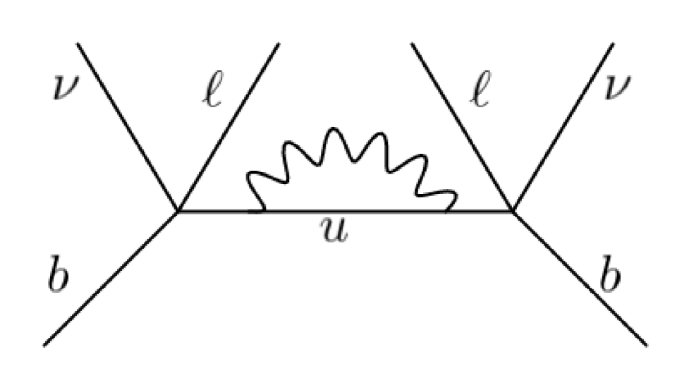
(a)

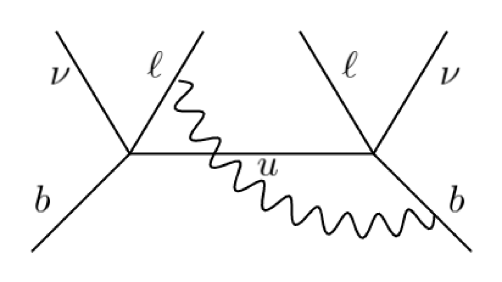
(b)

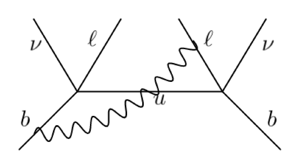
(c)

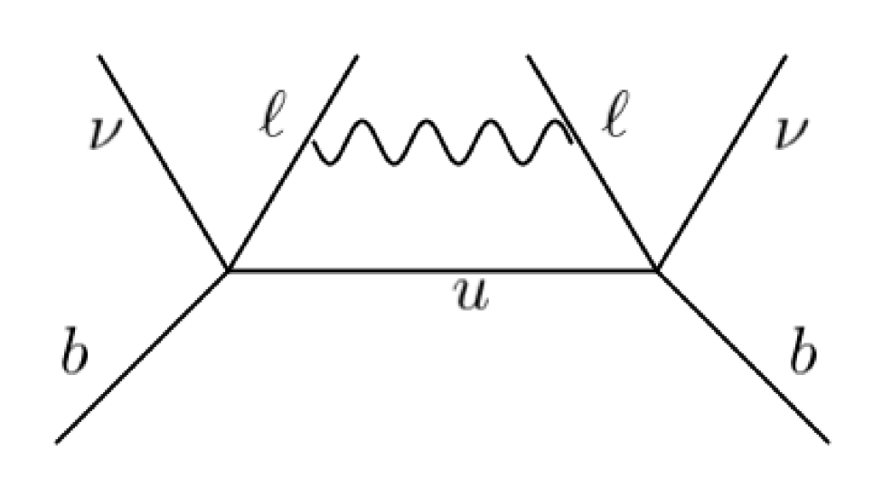
(d)

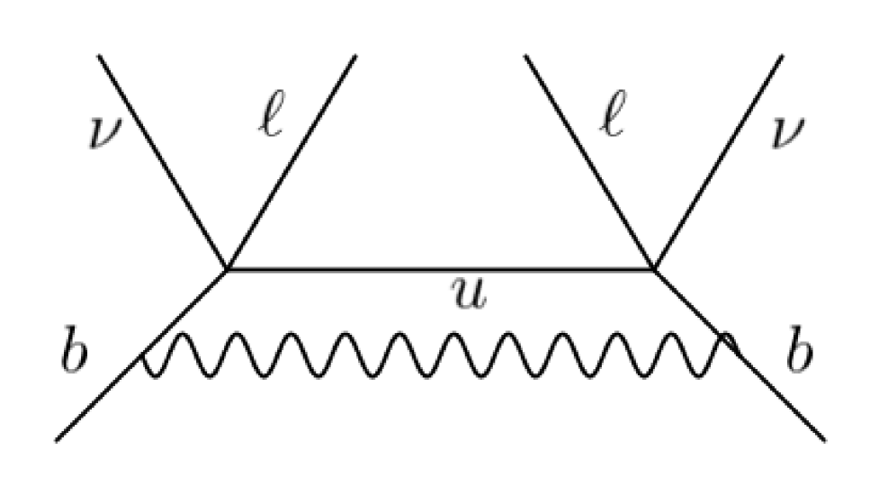
(e)

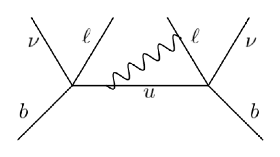
(f)

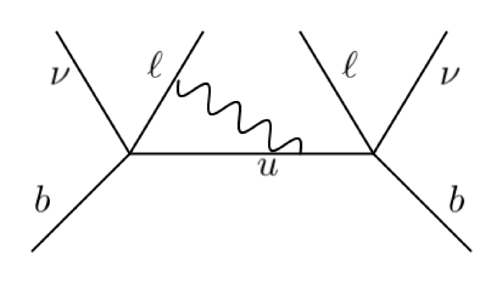
(g)

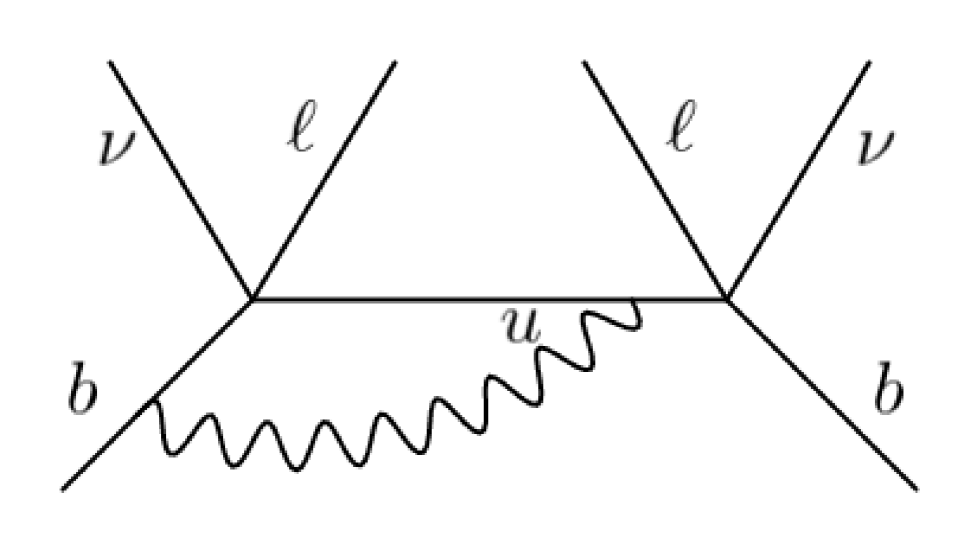
(h)

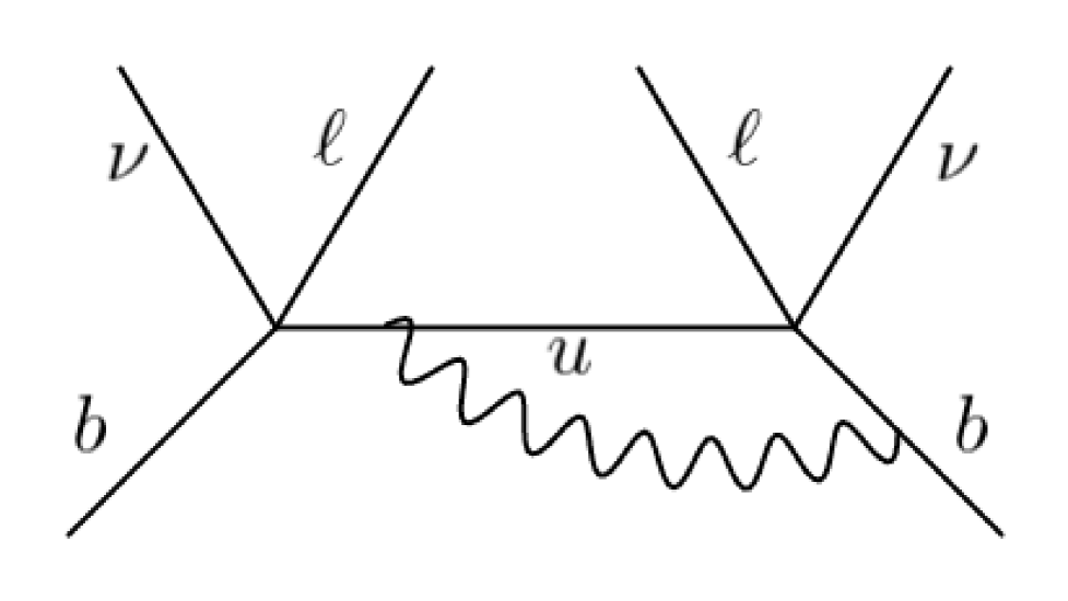
(i)

Figure 2: Feynman diagrams for $B\to X_{u}\ell\nu_{\ell}\gamma$.

Similar to Section-2, our focus is on the $B\to B$ forward scattering matrix element instead of the amplitude for $B\to X_{u}\ell\nu_{\ell}\gamma$ itself. The imaginary part of the amplitude shown in Fig.(3) is related to the inclusive rate for the $B\to X_{u}\ell\nu_{\ell}\gamma$ transition, as dictated by the optical theorem. However, the process $B\to X_{u}\ell\nu_{\ell}\gamma$ is highly non-trivial compared to the $B\to X_{u}\ell\nu_{\ell}$ mode due to the presence of a photon line between the charged quarks and leptons, as shown in Fig.(2). This means that some diagrams, such as Figs.2(b), 2(c), do not easily separate into leptonic and hadronic parts like in the $B\to X_{u}\ell\nu_{\ell}$ mode. Since the hadronic part in some of the diagrams communicates with the leptonic part through the photon, the calculation of the matrix element is more complex when expressed in terms of invariant tensors and using analytic properties of the transition operator. Also, in the present case, the transition tensor will be a four index object, two for the weak currents and two for the electromagnetic currents representing the photon emission. Therefore, it is more straightforward to use the Cutkosky method directly to compute the matrix element. As we verified in the last section, this method reproduces correct results for the decay rate of $B\to X_{u}\ell\nu_{\ell}$ mode.

Now, the decay rate for the semi-leptonic inclusive process $B\to X_{u}\ell\nu_{\ell}\gamma$ is given by

$$\Gamma_{\gamma}=\Big{(}\frac{4G_{F}}{\sqrt{2}}\Big{)}^{2}|V_{ub}|^{2}\frac{1}{2m_{B}}\int\frac{d^{3}p_{l}}{(2\pi)^{3}2E_{l}}\int\frac{d^{3}p_{\nu}}{(2\pi)^{3}2E_{\nu}}\int\frac{d^{4}k}{(2\pi)^{4}}Im\Big{[}\langle B|I\mathcal{M}_{\mu\nu}\mathcal{L}^{\mu\nu}|B\rangle\Big{]}$$ (19)

with

$$I\mathcal{M}_{\mu\nu}\mathcal{L}^{\mu\nu}=\sum_{m=1}^{9}I_{m}\mathcal{M}_{\mu\nu}^{(m)}\mathcal{L}^{\mu\nu(m)}$$ (20)

where, $\mathcal{M}_{\mu\nu}^{(m)}$ and $\mathcal{L}_{\mu\nu}^{(m)}$ contain the Dirac structure for quark and leptonic part respectively, and, $I_{m}$ contains denominator part of the propagator. Also, $m=1,...9$ corresponds to Fig. 2 $(a),...(i)$. $k$ is photon four momentum, $p_{\ell(\nu)}$ is lepton (neutrino) four momentum. The explicit calculation of forward scattering operator for Fig 2 (a) is presented below. All other diagrams can be calculated analogously. Calculating the hadronic and leptonic tensors requires the computation of $\mathcal{M}_{\mu\nu}^{(m)}$, $\mathcal{L}_{\mu\nu}^{(m)}$, and $I_{m}$. At the leading order in $\alpha_{s}$, the explicit forms of $\mathcal{M}_{\mu\nu}^{(1)}$, $\mathcal{L}_{\mu\nu}^{(1)}$, and $I_{1}$ are

$$\mathcal{M}_{\mu\nu}^{(1)} = 2(-ig^{\alpha\beta})\bar{b}\gamma^{\nu}\left(1-\gamma^{5}\right)i\left(\not{p_{b}}+\not{\Pi}-\not{q}\right)(-ieQ_{u})\gamma^{\alpha}i\left(\not{p_{b}}+\not{\Pi}-\not{k}-\not{q}+m_{u}\right)(-ieQ_{u})\gamma^{\beta}i\big{(}\not{p_{b}}$$

$$+ \not{\Pi}-\not{q}\big{)}\gamma^{\mu}\left(1-\gamma^{5}\right)b,$$

$$\mathcal{L}_{\mu\nu}^{(1)} = \left(\bar{\ell}\gamma^{\mu}(1-\gamma^{5})\nu_{\ell}\right)\left(\bar{\nu}_{\ell}\gamma^{\nu}(1-\gamma^{5})\ell\right),$$ (21)

and

$$I_{1} = \frac{1}{(k^{2}+i\epsilon)((p_{b}+\Pi-q)^{2}-m_{u}^{2}+i\epsilon)((p_{b}+\Pi-q-k)^{2}-m_{u}^{2}+i\epsilon)((p_{b}+\Pi-q)^{2}-m_{u}^{2}+i\epsilon)}$$ (22)

respectively. As before, the effective momentum of $b$ quark is given by $p_{b}+\Pi$. Expanding $I_{1}$ in powers of $\Pi$ yields an expansion in terms of $\frac{\Lambda_{\text{QCD}}}{m_{b}}$, similar to the $B\to X_{u}\ell\nu_{\ell}$ mode. The explicit form of $I_{1}$ up to $\mathcal{O}(\Pi^{2})$ is obtained from Eqn.(22), and is given by

$$I_{1} = \frac{1}{k^{2}((p_{b}-q-k)^{2}-m_{u}^{2})}\Big{[}\frac{1}{(p_{u}.k)^{2}}-\frac{2(p_{b}-q).\Pi}{(p_{u}.k)^{3}}-\frac{\Pi^{2}}{(p_{u}.k)^{3}}+\frac{2((p_{b}-q).\Pi)^{2}}{(p_{u}.k)^{4}}\Big{]}$$ (23)

$$- \frac{1}{k^{2}((p_{b}-q-k)^{2}-m_{u}^{2})^{2}}\Big{[}\frac{2p_{u}.\Pi}{(p_{u}.k)^{2}}-\frac{4(p_{u}.\Pi)(p_{b}-q).\Pi}{(p_{u}.k)^{3}}-\frac{\Pi^{2}}{(p_{u}.k)^{2}}\Big{]}$$

$$+ \frac{1}{k^{2}((p_{b}-q-k)^{2}-m_{u}^{2})^{3}}\Big{[}\frac{2(p_{u}.\Pi)^{2}}{(p_{u}.k)^{2}}\Big{]}$$

Similar to Section-2, the Cutkosky method is exploited (see Fig.(3)) to calculate the imaginary part of the matrix element.

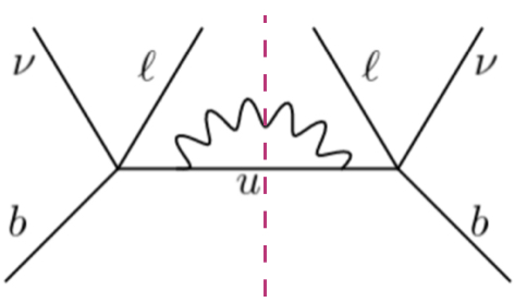
Figure 3: Representative diagram with explicit cut

Mathematically, this essentially replaces the cut propagator by a product of delta function and theta function enforcing the positive energy condition. For example

$$\frac{1}{((p_{b}-q-k)^{2}-m_{u}^{2}+i\epsilon)}\to(-2\pi i)\delta((p_{b}-q-k)^{2}-m_{u}^{2})\Theta((p_{b}^{0}-q^{0}-k^{0})).$$ (24)

More generally one has the identity

$$-\frac{1}{\pi}Im\Big{(}\frac{1}{(p_{b}-q-k)^{2}-m_{u}^{2}}\Big{)}^{n}=\frac{(-1)^{(n-1)}}{(n-1)!}\delta^{(n-1)}((p_{b}-q-k)^{2}-m_{u}^{2}),$$ (25)

where the superscript of the delta function denotes $(n-1)$th derivative with respect to its argument itself. When working with terms involving the derivatives of the delta function, it is important to handle them with care. The first step is to use integration by parts to remove the derivatives from the delta function and transfer them on to other functions multiplying it. However, it is crucial to use the theta function carefully during this process because it determines the minimum value of the neutrino energy, denoted by $E_{\nu}$. See Appendix B for details of kinematics.

Subsequently, we proceed by combining the terms $\mathcal{M}{\mu\nu}^{(1)}$, $\mathcal{L}{\mu\nu}^{(1)}$, and $I_{1}$ to compute the imaginary part of the amplitude. Notably, our analysis reveals that no new operators are produced beyond those already present in the decay rate of the $B\to X_{u}\ell\nu_{\ell}$ process. All the pertinent operators, up to dimension five, are listed in Eqn.(14).

It is evident that only $I_{1}$ contributes to the imaginary part of the matrix element. Hence, we have presented an explicit expression of the matrix element in accordance with the representation outlined in Eqn.(23). Each square bracket contains terms with expansion in $\Pi$ up to second order. The imaginary parts of the coefficients of these square brackets contribute to the delta function and its derivatives. We designate the forward scattering matrix element as

$$\mathcal{J}_{1}(n;\alpha)=\langle B(v)|Im\{I_{1}\mathcal{M}_{\mu\nu}^{(1)}\mathcal{L}_{\mu\nu}^{(1)}\}|B(v)\rangle(n\alpha).$$ (26)

Where, $n=0,1,2$ denotes expansion powers of $\Pi$ and $\alpha=a,c,d$ represents square brackets of Eqn.(23) in order. For example in $\mathcal{J}(0;a)$, ${}^{\prime}0^{\prime}$ denotes the expansion in $\Pi$ to $\mathcal{O}(\Pi^{0})$ and ${}^{\prime}a^{\prime}$ tells that elements of first square bracket of Eqn.(23) are chosen. We now explicitly list all the the expressions for each of the terms of $I_{1}$ without the delta function or its derivatives.

$$\mathcal{O}(\Pi^{0}):$$

$$\mathcal{J}_{1}(0;a) = \frac{-1}{m_{b}(p_{u}.k)^{2}}16(p_{b}.p_{\ell})\Big{(}(q^{2}+m_{b}^{2}-2(p_{b}.q))(p_{\nu}.(p_{b}+k-q))-2((p_{b}-q).k)(q-p_{b}).p_{\nu}\Big{)}$$ (27)

$$\mathcal{O}(\Pi):$$

$$\mathcal{J}_{1}(1;a) = \frac{-1}{3m_{b}^{3}(p_{u}.k)^{3}}64(\lambda_{1}+3\lambda_{2})\Big{(}2m_{b}^{2}(p_{\ell}.q)+(p_{b}.p_{\ell})(3m_{b}^{2}-5(p_{b}.q))\Big{)}\Big{(}(q^{2}+m_{b}^{2}-2(p_{b}.q))$$ (28)

$$(p_{\nu}.(p_{b}+k-q))-2((p_{b}-q).k)(p_{\nu}.q-p_{b}.p_{\nu})\Big{)}$$

$$\mathcal{O}(\Pi^{2}):$$

$$\mathcal{J}_{1}(2;a) = \frac{1}{3m_{b}^{3}(p_{u}.k)^{4}}32\lambda_{1}(p_{b}.p_{\ell})\Big{(}-2(p_{u}.k)^{2}(m_{b}^{2}(p_{\nu}.k-5(p_{\nu}.q))+(p_{b}.p_{\nu})(2(p_{b}.(q+k))+3m_{b}^{2}))$$ (29)

$$+ ((q^{2}+m_{b}^{2}-2(p_{b}.q))(p_{\nu}.(p_{b}+k-q))-2(p_{b}-q).k((p_{b}-q).p_{\nu}))((p_{b}.q)^{2}+m_{b}^{2}(3(p_{u}.k)-q^{2}))$$

$$+ 4(p_{u}.k)\Big{(}m_{b}^{2}((p_{\ell}.p_{\nu})(2p_{b}.(q+k)-4(q.k)-3q^{2})+(p_{b}.p_{\nu})(p_{b}.q+2(q.k+q^{2}))+2q^{2}(p_{\nu}.k))$$

$$+ (p_{b}.q)(2(p_{\nu}.q)(p_{b}.(q+k))-2(p_{b}.q)(p_{\nu}.k)+(p_{b}.p_{\nu})(q^{2}+2(q.k)-4p_{b}.(q+k)))-m_{b}^{4}(p_{\nu}.q))\Big{)}\Big{)}$$

The sum, $\mathcal{J}_{1}(0;a)+\mathcal{J}_{1}(1;a)+\mathcal{J}_{1}(2;a)$, is multiplied with $\delta(k^{2})\theta(k^{0})\delta(((p_{b}-q-k)^{2}-m_{u}^{2}))\theta((p_{b}-q-k)^{0})$. Similarly, the second square brackets of Eqn.(23) with hadronic and leptonic tensors (Eqn.(21)) produce the terms expanded in powers of $\Pi$. Since this set of terms comes multiplied with $\frac{1}{((p_{b}-q-k)^{2}-m_{u}^{2})^{2}}$ i.e. square of the propagator, the sum of these terms has an overall factor of $\delta(k^{2})\theta(k^{0})\delta^{\prime}(((p_{b}-q-k)^{2}-m_{u}^{2}))\theta((p_{b}-q-k)^{0})$.

$$\mathcal{O}(\Pi):$$

$$\mathcal{J}_{1}(1;c) = \frac{-1}{3m_{b}^{3}(p_{u}.k)^{2}}128(\lambda_{1}+3\lambda_{2})\Big{(}(m_{b}^{2}+q^{2}-2p_{b}.q)((p_{b}-q+k).p_{\nu})-2((p_{b}-q).k)((p_{b}-q).p_{\nu})\Big{)}$$ (30)

$$\Big{(}(p_{b}.p_{\ell})(5p_{b}.(q+k)-3m_{b}^{2})-2m_{b}^{2}(p_{\ell}.(q+k))\Big{)}$$

$$\mathcal{O}(\Pi^{2}):$$

$$\mathcal{J}_{1}(2;c) = \frac{-1}{3m_{b}^{3}(p_{u}.k)^{3}}128\Big{(}\lambda_{1}(p_{b}.p_{\ell})\Big{(}8((p_{u}.k+p_{b}.q)(p_{\nu}.q)--(2(p_{u}.k)+p_{b}.q)(p_{b}.p_{\nu}))(p_{b}.k)^{2}$$ (31)

$$+ 2\Big{(}(4(p_{\nu}.k)(p_{u}.k)+(7p_{u}.k-4k.q-4q^{2})(p_{\nu}.q)+(4(q.k)-3(p_{u}.k)+4q^{2})(p_{b}.p_{\nu}))m_{b}^{2}$$

$$- 2(p_{b}.q)((p_{\nu}.k)(2(p_{u}.k)-q^{2}+2(p_{b}.q)-m_{b}^{2})+(p_{\nu}.q)(2k.q-4(p_{u}.k)+q^{2}-4(p_{b}.q)+m_{b}^{2}))$$

$$+ 2(2(q.k)(p_{u}.k+p_{b}.q)+(p_{u}.k)(q^{2}-8(p_{b}.q)+m_{b}^{2})+(p_{b}.q)(q^{2}-4(p_{b}.q)+m_{b}^{2}))(p_{b}.p_{\nu}))(p_{b}.k)$$

$$+ \Big{(}8(p_{b}-p_{\nu}).q(k.q)^{2}+2(2(3q^{2}-2(q.p_{b})+m_{b}^{2})(p_{\nu}.q-p_{b}.p_{\nu})+p_{u}.k(11(p_{b}.p_{\nu})-15(q.p_{\nu})))(k.q)$$

$$+ 4q^{2}(q^{2}-2(p_{b}.q)-m_{b}^{2})(p_{b}-q).p_{\nu}+p_{u}.k((2(p_{b}.q)-m_{b}^{2})(7q-3p_{b}).p_{\nu}+q^{2}(11p_{b}-15q).p_{\nu})\Big{)}m_{b}^{2}$$

$$+ 4(p_{b}.q)\Big{(}p_{b}.qp_{\nu}.q(2(p_{u}-q).k-q^{2}+2p_{b}.q-m_{b}^{2})+(2(q.k)(p_{u}.k+p_{b}.q)+p_{u}.k(q^{2}-4p_{b}.q+m_{b}^{2})$$

$$+ p_{b}.q(q^{2}-2p_{b}.q+m_{b}^{2}))(p_{b}.p_{\nu})\Big{)}+(p_{\nu}.k)\Big{(}4(q^{2}-2p_{b}.q+m_{b}^{2})((p_{b}.q)^{2}-(q^{2}+k.q)m_{b}^{2})$$

$$+ (p_{u}.k)((7q^{2}+2p_{b}.q-m_{b}^{2})m_{b}^{2}-8(p_{b}.q)^{2})\Big{)}\Big{)}\Big{)}$$

In a similar way, we then consider the imaginary part of the third square bracket of Eqn. (23), and combine with Eqn. (21). Explicitly the amplitude in the expanded in powers of $\Pi$ is

$$\mathcal{O}(\Pi^{2}):$$

$$\mathcal{J}_{1}(2;d) = \frac{1}{3m_{b}^{3}(p_{u}.k)^{2}}256\lambda_{1}(p_{b}.p_{\ell})\Big{(}(-2p_{b}.q+m_{b}^{2}+q^{2})(p_{b}+k-q).p_{\nu}-2(p_{b}-q).k(q-p_{b}).p_{\nu}\Big{)}$$ (32)

$$\Big{(}((q+k).p_{b})^{2}-m_{b}^{2}(2q.k+q^{2})\Big{)}.$$

Here, $`d^{\prime}$ refers to the elements of the third square bracket of Eqn. (23). Moreover, the $\mathcal{J}_{1}(2;d)$ has a multiplicative factor of $\delta(k^{2})\theta(k^{0})\delta^{\prime\prime}(((p_{b}-q-k)^{2}-m_{u}^{2}))\theta((p_{b}-q-k)^{0})$.

Next, combining all the amplitudes, the total forward matrix element for Fig.2(a) is given by

$$\langle B|Im\{I_{1}\mathcal{M}_{\mu\nu}^{(1)}\mathcal{L}_{\mu\nu}^{(1)}|B\}\rangle = \delta(k^{2})\theta(k^{0})\Big{[}(\mathcal{J}_{1}(0;a)+\mathcal{J}_{1}(1;a)+\mathcal{J}_{1}(2;a))\delta((p_{b}-q-k)^{2}-m_{u}^{2})+(\mathcal{J}_{1}(1b)+\mathcal{J}_{1}(2b))$$ (33)

$$\delta^{\prime}((p_{b}-q-k)^{2}-m_{u}^{2})+(\mathcal{J}_{1}(2;c))\delta^{\prime\prime}((p_{b}-q-k)^{2}-m_{u}^{2})\Big{]}\theta((p_{b}-q-k)^{0})$$

Integration by parts is then used to simplify such expressions;

$$\delta^{\prime}(x)\theta(x)f(x) = -\delta(x)\delta(x)f(x)-\delta(x)\theta(x)f^{\prime}(x),\ \text{and}$$ (34)

$$\delta^{\prime\prime}(x)\theta(x)f(x) = \delta(x)\delta^{\prime}(x)f(x)+2\delta(x)\delta(x)f^{\prime}(x)+\delta(x)+\theta(x)f^{\prime\prime}(x).$$ (35)

These relations will be used to carry out integrals over phase space. In a similar way, the forward matrix elements for the remaining eight Feynman diagrams as shown in Fig.(2) are calculated. Relevant expressions for $\mathcal{M}_{\mu\nu}^{(m)}$, $\mathcal{L}_{\mu\nu}^{(m)}$, and $I_{m}$ $m=2,...9$ for all the Feynman diagrams are provided in Appendix A.

4 Results

As a general rule, the four-body phase space comprises of five distinct variables. In the context of inclusive decays, we have an additional variable, namely the invariant mass squared of the final state meson $(p_{X}^{2})$, which we trade for $q^{\prime 2}\ (=(p_{\ell}+p_{\nu}+k)^{2})$. The other independent variables are the lepton energy $y\ (=\frac{2p_{b}.p_{\ell}}{m_{B}^{2}})$, the energy of the hard photon $x\ (=\frac{2p_{b}.k}{m_{B}^{2}})$, the neutrino energy, and three angles. These are defined in the rest frame of the $B$ meson. A detailed description of the kinematics is furnished in Appendix B.

We begin by integrating over all variables except $y$ to determine the spectrum of the charged lepton for different values of $x$. Fig. (4(a)) illustrates the differential decay rate as a function of the lepton energy ($y$) for various photon energy values ($x$). We observe that as the photon becomes increasingly soft, the leptonic energy end point shifts accordingly, which is consistent with the kinematics of the process.

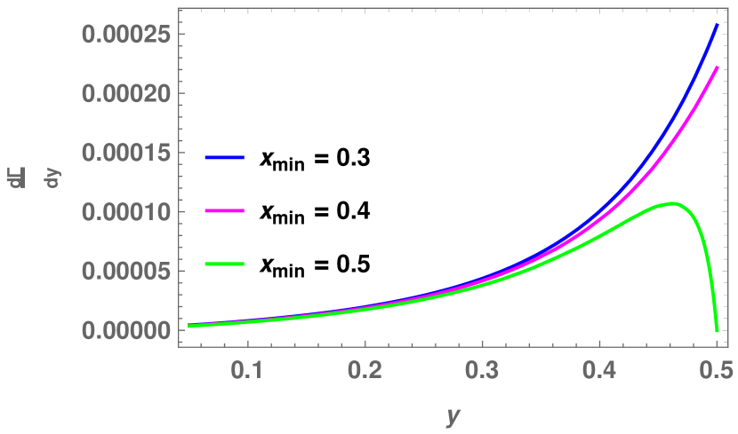
(a)

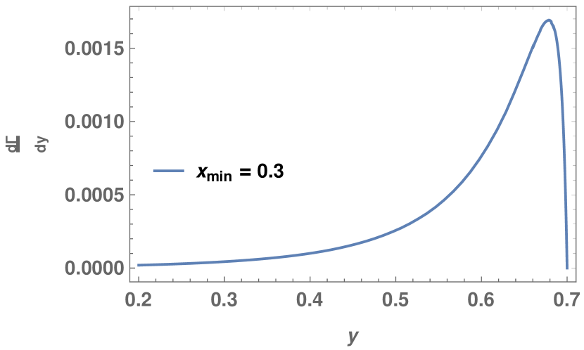
(b)

Figure 4: (a) : Differential decay width of $B\to X_{u}\mu\nu_{\mu}\gamma$ for different value of normalized photon energy ($x$), and (b) : Differential decay width of $B\to X_{u}\mu\nu_{\mu}\gamma$ for particular normalized photon energy ($x_{min}=0.3$).

To provide a complete picture of the distribution for the differential decay rate, we present the distribution for $x_{min}=0.3$ which corresponds to $k_{min}\sim 0.8\ GeV$ in Fig.(4(b)). The plot shows that the distribution ends at the kinematical boundary which is, as expected, larger than that for $x_{min}=0.5$, and more towards non-readiative, $B\to X_{u}\ell\nu_{\ell}$, case.

Further, as an example of possible additional observable, we define the photon (differential) forward-backward asymmetry, $A_{FB}(y)$, with respect to recoiling final state hadron as

$$A_{FB}(y)=\frac{\int_{0}^{1}dt\frac{d^{2}\Gamma_{\gamma}}{dydt}-\int_{-1}^{0}dt\frac{d^{2}\Gamma_{\gamma}}{dydt}}{\int_{-1}^{1}dt\frac{d^{2}\Gamma_{\gamma}}{dydt}}$$ (36)

where $t=cos\theta_{X\gamma}$ is the angle between the outgoing photon and recoiling hadron ($X$) in the rest frame of $B$ meson. The forward-backward asymmetry is shown in Fig.(5) for $\lambda_{1}=-0.2$ and $\lambda_{2}=0.12$.

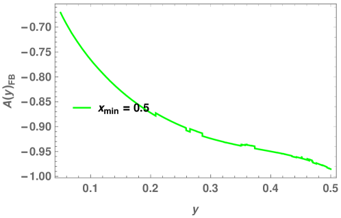
Figure 5: Forward-backward asymmetry ($A_{FB}$) with lepton energy (y).

Finally, Fig.(6) depicts the differential decay rate as a function of the normalized photon energy ($x$), which shows that with lowering of the energy of the photon, the decay rate behaves as for the non-radiative mode.

It is worth noting that infrared divergences can be effectively circumvented by assigning sufficient mass to the photon i.e. the photon is made sufficiently hard. To avoid any contribution from mass singularities, we choose to work with muons in the final state. Furthermore, by choosig a lower cut for the polar angle, we can eliminate any collinear singularities that might arise.

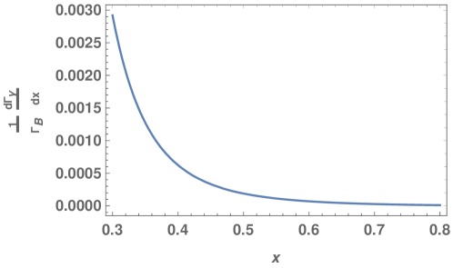
Figure 6: Differential decay width of $B\to X_{u}\mu\nu_{\mu}\gamma$ with photon energies ($x$).

For $B\to X_{u}\mu\nu_{\mu}\gamma$, where the photon is hard, the total decay width ($\Gamma_{\gamma}$) for the radiative mode is expected to be suppressed by $\mathcal{O}(\alpha)$ compared to the total decay width for $B\to X_{u}\mu\nu_{\mu}$. In order to check if this expectation is met, we evaluate the ratio of the radiative decay width ($\Gamma_{\gamma}$) to the non-radiative decay width ($\Gamma$). We find that this ratio is approximately $0.01$ for hard photons with energy around $1$GeV ($x_{min}=0.5$), thus confirming the expectation.

4.1 Non-perturbative parameters

After determining the decay width, we now propose a simple yet efficient method for calculating the non-perturbative parameters $\lambda_{1}$ and $\lambda_{2}$. We observe that using the ratio of the decay widths, instead of the widths themselves, is more suitable since the latter may contain uncertainties due to the CKM element $V_{ub}$. Moreover, such ratios yield ratios of simple functions of $\lambda_{1}$ and $\lambda_{2}$. By knowing the experimentally measured values of $R_{1}$ and $R_{2}$, we can simultaneously solve these two linear equations to obtain $\lambda_{1}$ and $\lambda_{2}$. The two ratios that we propose to employ are as in Eqn.(4). Both numerator and denominator have the form $A+B\lambda_{1}+C\lambda_{2}$. Thus each of the ratios has the form

$$\frac{A+B\lambda_{1}+C\lambda_{2}}{A^{\prime}+B^{\prime}\lambda_{1}+C^{\prime}\lambda_{2}}=R_{1}\ \text{(say)}$$ (37)

and same for $R_{2}$. These are still two linear equations in $\lambda_{1}$ and $\lambda_{2}$. To further illustrate the practicality of our proposed method, we perform a sample calculation for non-perturbative parameters $\lambda_{1}$ and $\lambda_{2}$. At this point, there is no data available to directly determine $\lambda_{1}$ and $\lambda_{2}$. To proceed further in order to demonstrate the case of obtaining $\lambda_{1}$ and $\lambda_{2}$ once the suggested ratios are experimentally available, we obtain a value for $R_{2}$ using the known values of $\lambda_{1}$ and $\lambda_{2}$, and for $R_{1}$ we choose it to be $\alpha_{em}R_{2}$. With these values, we can then numerically calculate the non-perturbative parameters $\lambda_{1}$ and $\lambda_{2}$. Our results yield $\lambda_{1}=-0.24$ $GeV^{2}$ and $\lambda_{2}=0.15$ $GeV^{2}$, which are consistent with previously values reported in the literature [22, 24]: $\lambda_{1}=-0.19\pm 0.10$ $GeV^{2}$ and $\lambda_{2}=0.12\pm 0.01$ $GeV^{2}$. This motivates the need for a measurement of experimental measurement of the decay width of $B\to X_{u}\ell\nu_{\ell}\gamma$. Such a determination will aid in precise determination of $\lambda_{1}$ and $\lambda_{2}$. As mentioned earlier, we have focused on $\mathcal{O}(\frac{1}{m_{b}})$ terms in HQE and therefore are sensitive only to $\lambda_{1}$ and $\lambda_{2}$ (or $\mu_{\pi}^{2}$ and $\mu_{G}^{2}$). At higher orders, the expressions develop dependence on more such non-perturbative parameters. Measurements of $B\to X_{u}\ell\nu_{\ell}\gamma$ rate and ratio $R_{1}$ will infact be very helpful in a simultaneous and easy determination of these parameters when combined with $B\to X_{u}\ell\nu_{\ell}$ data and ratio $R_{2}$.

5 Summary

To summarize, we have proposed a method to calculate the non-perturbative parameters $\lambda_{1}$ and $\lambda_{2}$ in the context of inclusive $B$ meson decays. We first calculated the decay width for the inclusive modes $B\to X_{u}\ell\nu_{\ell}$ and $B\to X_{u}\ell\nu_{\ell}\gamma$ directly using the Cutkosky method and the heavy qaurk expansion applied to the amplitude, retaining terms to order $(\frac{\Lambda_{QCD}}{m_{b}})$ in HQE. Since the radiative mode, $B\to X_{u}\ell\nu_{\ell}\gamma$, involves a hard photon, the most general tensorial structure will involve four indices as opposed to two for $B\to X_{u}\ell\nu_{\ell}$. In view of this and related complications to pick out the analytic properties in order to evaluate decay rate, we decided to compute the relevant amplitude directly (or brute force) by using Cutkosky method. The differential rate contains two non-perturbative parameters $\lambda_{1}$ and $\lambda_{2}$. Further, the differential and total decay rates were then obtained by integrating over the four-body phase space variables. The differential rate and forward-backward asymmetry are plotted with respect to lepton energy for different $x_{min}$ values that define the hardness of the photon. It was found that the decay rate for radiative mode ($B\to X_{u}\ell\nu_{\ell}\gamma$) is $\mathcal{O}(\alpha)$ times non-radiative mode ($B\to X_{u}\ell\nu_{\ell}$) when the photon is sufficiently hard.

Next, two ratios, $R_{1}$ and $R_{2}$, are formed using the differential rate for radiative (for photon energy $\geq\ \text{few times}\ \Lambda_{QCD}\sim 500MeV$) and non-radiative modes respectively, in different lepton energy ranges. These ratios are independent of the CKM element and provide two linear equations in $\lambda_{1}$ and $\lambda_{2}$, allowing an unambiguous determination of these parameters. A simple example is also shown in Section-4.1 to demonstrate the calculation of the these parameters, $\lambda_{1}$ and $\lambda_{2}$, which are found to be consistent with existing values. It should be mentioned that at present the radiative mode has not been measured. The results of this exercise encourage us to have precise measurements of the radiative mode, more so since at higher orders in HQE, there are more non-perturbative parameters that enter the amplitude. The radiative inclusive semi-leptonic mode will be very useful in aiding a clean determination of these.

The decay rate for free quark decay in $B\to X_{u}\ell\nu{\ell}$ $\propto 2y^{2}(2y-3)$, where $y$ is the normalized lepton energy in the rest frame of $B$ meson. This indicates the difference in partonic and hadronic end points, with former being $\frac{m_{b}}{2}$ and the latter being at $\frac{m_{B}}{2}$, resulting in an end point region of order $\bar{\Lambda}=m_{B}-m_{b}$. In order to correctly include this region, it is required to sum over the infinite terms present in the heavy quark expansion. However, this expansion in $\frac{\bar{\Lambda}}{m_{b}}$ brings higher-order derivatives of delta function at each successive order resulting in a failure of OPE and QCD perturbation theory in this region. Therefore in order to incorporate the end-point behaviour, the distribution function of the heavy quark or the shape function, needs to be introduced in the decay rate of $B\to X_{u}\ell\nu{\ell}$ and $B\to X_{s}\gamma$ mode [13, 10].

Now, in the case of radiative decay ($B\to X_{u}\ell\nu_{\ell}\gamma$) mode, it is noted that the presence of a hard photon in the final state causes the endpoint to shift in comparison to the non-radiative decay. The partonic and hadronic end points are at $\frac{m_{b}}{2}-x_{min}$ and $\frac{m_{B}}{2}-x_{min}$ respectively. However, the challenge due to the difference in partonic and hadronic endpoints remains similar to $B\to X_{u}\ell\nu_{\ell}$ mode. Hence, the shape function for this process is required. Further, one can try to use a simple form of the shape function, $\propto(1-y-x)^{a}e^{(1+a)(x+y)}$, similar to the one suggested for non-radiative decay mode [25, 26]. However, this may be very naive at this point, and hence it is required to compute the shape function for this process and verify its universality before any definitive conclusions can be drawn. While the issue of the form of the shape function remains unsettled at this point, and is left for a future study, the main idea that the use of radiative inclusive decay rate can aid in a quick determination of $\lambda_{1}$ and $\lambda_{2}$ stays unaffected.

In conclusion, our proposed method provides a simple yet efficient way to calculate non-perturbative parameters $\lambda_{1}$ and $\lambda_{2}$ in inclusive $B$ decays once the decay rate for radiative $B\to X_{u}\ell\nu_{\ell}\gamma$ is known experimentally.

Appendix A Contributions from different diagrams to the inclusive Matrix Element

The explicit structure of $\mathcal{M}_{\mu\nu}^{(m)}$, $\mathcal{L}_{\mu\nu}^{(m)}$ and $I_{m}$ are listed below. All the relevant expressions for Fig.2(a) are listed in Section-3. We now present explicit expressions for diagrams Fig.2(b) to Fig.2(i).

1. Fig.2(b):

$$\mathcal{M}_{\mu\nu}^{(2)} = 2(-ig^{\alpha\beta})\bar{b}(-ieQ_{b})\gamma_{\alpha}i\left(\not{p_{b}}+\not{\Pi}-\not{k}+m_{b}\right)\gamma^{\nu}(1-\gamma^{5})i\left(\not{p_{b}}+\not{\Pi}-\not{k}-\not{q}+m_{u}\right)\gamma^{\mu}\left(1-\gamma^{5}\right)b$$

$$\mathcal{L}_{\mu\nu}^{(2)} = \left(\bar{\ell}(-ieQ_{\ell})\gamma_{\beta}i\left(\not{p_{l}}+\not{k}+m_{l}\right)\gamma^{\mu}(1-\gamma^{5})\nu_{\ell}\right)\left(\bar{\nu}_{\ell}\gamma^{\nu}(1-\gamma^{5})\ell\right)$$ (38)

$$I_{2} = \frac{1}{k^{2}((p_{b}-q-k)^{2}-m_{u}^{2})}\Big{[}\frac{-1}{(p_{b}.k)(p_{\ell}.k)}-\frac{(p_{b}-k).\Pi}{(p_{\ell}.k)(p_{b}.k)^{2}}-\frac{\Pi^{2}}{2(p_{\ell}.k)(p_{b}.k)^{2}}-\frac{((p_{b}-k).\Pi)^{2}}{2(p_{\ell}.k)(p_{b}.k)^{3}}\Big{]}$$ (39)

$$- \frac{1}{k^{2}((p_{b}-q-k)^{2}-m_{u}^{2})^{2}}\Big{[}\frac{2p_{u}.\Pi}{(p_{\ell}.k)(p_{b}.k)}+\frac{2(p_{u}.\Pi)(p_{b}-k).\Pi}{(p_{\ell}.k)(p_{b}.k)^{2}}+\frac{\Pi^{2}}{(p_{\ell}.k)(p_{b}.k)}\Big{]}$$

$$- \frac{1}{k^{2}((p_{b}-q-k)^{2}-m_{u}^{2})^{3}}\Big{[}\frac{2(p_{u}.\Pi)^{2}}{(p_{\ell}.k)(p_{b}.k)}\Big{]}$$

$$\mathcal{O}(\Pi^{0}):$$

$$\mathcal{J}_{2}(0;a) = \frac{-1}{m_{b}(p_{b}.k)(p_{\ell}.k)}16\Big{(}-2(p_{b}.p_{\nu})\Big{(}2(p_{b}.p_{\ell})^{2}+(p_{\ell}.k)^{2}+p_{\ell}.k(p_{b}.q+p_{\ell}.q-3p_{b}.p_{\ell})-(p_{b}.k)(p_{\ell}.k)$$ (40)

$$- p_{b}.p_{\ell}(q.k-2p_{b}.k+2p_{\ell}.q)\Big{)}+m_{b}^{2}\Big{(}p_{\ell}.k((p_{b}+q).p_{\nu})+p_{\ell}.p_{\nu}(p_{b}.k-q.k-2p_{\ell}.k)$$

$$- ((q-p_{b}).p_{\ell})(p_{\nu}.k+2p_{\ell}.p_{\nu})\Big{)}-2((p_{b}.p_{\ell})(p_{\nu}.k)-(p_{b}.k)(p_{\ell}.p_{\nu}))((q+k-p_{b}).p_{\ell})\Big{)}$$

$$\mathcal{O}(\Pi):$$

$$\mathcal{J}_{2}(1;a) = \frac{-1}{3m_{b}^{3}(p_{b}.k)^{2}(p_{\ell}.k)}32(\lambda_{1}+3\lambda_{2})\Big{(}2m_{b}^{2}\Big{(}p_{\nu}.k\big{(}p_{b}.p_{\ell}(p_{\ell}.q-2q.k-3p_{\ell}.k)-(p_{b}.p_{\ell})^{2}$$ (41)

$$+ 2p_{\ell}.k(p_{b}.q+2p_{\ell}.k+2p_{\ell}.q)\big{)}+p_{b}.p_{\nu}\big{(}6(p_{b}.p_{\ell})^{2}-p_{b}.p_{\ell}(7p_{\ell}.k+3q.k+6p_{\ell}.q)$$

$$+ p_{\ell}.k(3p_{b}.q+p_{\ell}.(q+k))\big{)}\Big{)}+(p_{b}.k)^{2}\big{(}10(p_{\ell}.p_{\nu}(q+k-p_{b}).p_{\ell})+p_{b}.p_{\nu}(p_{\ell}.q-2p_{b}.p_{\ell})$$

$$+ m_{b}^{2}p_{\ell}.p_{\nu}\big{)}+p_{b}.k\Big{(}-10p_{b}.p_{\nu}\big{(}2(p_{b}.p_{\ell})^{2}-p_{b}.p_{\ell}(3p_{\ell}.k+q.k+2p_{\ell}.q)+p_{\ell}.k(p_{b}.q+(q+k).p_{\ell})\big{)}$$

$$+ m_{b}^{2}\big{(}p_{\nu}.k(9p_{b}-5q).p_{\ell}+p_{\ell}.k(9p_{b}-12p_{\ell}+q)-p_{\ell}.p_{\nu}(12(q-p_{b}).p_{\ell}+q.k)-6p_{b}.p_{\nu}(q-2p_{b}).p_{\ell}\big{)}$$

$$- 10(p_{b}.p_{\ell})(p_{\nu}.k)((q+k-p_{b}).p_{\ell})-3m_{b}^{4}(p_{\ell}.p_{\nu})\Big{)}+m_{b}^{4}\big{(}3(p_{b}-q).p_{\ell}((k+2p_{\ell}).p_{\nu})+3(q.k)(p_{\ell}.p_{\nu})$$

$$- 3(p_{\ell}.k)(p_{\nu}.(p_{b}-2p_{\ell}+q))+4p_{\nu}.k\big{)}\Big{)}$$

$$\mathcal{J}_{2}(1;c) = \frac{1}{3m_{b}^{3}(p_{b}.k)(p_{\ell}.k)}128(\lambda_{1}+3\lambda_{2})\Big{(}m_{b}^{4}\big{(}p_{\nu}.k((q-3p_{b}).p_{\ell})-p_{\ell}.k((4k+5q+3p_{b}-6p_{\ell}).p_{\nu})$$ (42)

$$+ p_{\ell}.p_{\nu}(5k.q+6p_{\ell}.q-6p_{b}.p_{\ell})\big{)}+\big{(}2((4k+2q+p_{b}).p_{\nu})(p_{\ell}.k)^{2}+\big{(}2p_{\nu}.k(2q.p_{b}+6q.p_{\ell}-3p_{b}.p_{\ell})$$

$$+ 4p_{\nu}.q((q-2p_{b}).p_{\ell})+2q^{2}(p_{b}.p_{\nu})-2((q+7p_{b}).p_{\ell})p_{b}.p_{\nu}+p_{b}.q((5q+11p_{b}-6p_{\ell}).p_{\nu})$$

$$- 4(q.k)(p_{\ell}.p_{\nu})\big{)}p_{\ell}.k+4(p_{\nu}.q)(p_{b}.p_{\ell})((p_{b}-q).p_{\ell})+p_{\nu}.k\big{(}4(q.p_{\ell})^{2}-2(p_{b}.p_{\ell})^{2}-p_{b}.q((q-5p_{b}).p_{\ell})$$

$$- 2p_{b}.p_{\ell}(2k.q+q^{2}+p_{\ell}.q)\big{)}-2p_{b}.p_{\nu}\big{(}2q.p_{\ell}((k+p_{\ell}).q)+p_{b}.p_{\ell}((3k+4p_{\ell}).q)-6(p_{b}.p_{\ell})^{2}\big{)}$$

$$+ p_{\ell}.p_{\nu}\big{(}6p_{b}.q((p_{b}-q).p_{\ell})+k.q(4p_{b}.p_{\ell}-4q.p_{\ell}-5q.p_{b})\big{)}\big{)}m_{b}^{2}+10q.p_{b}\big{(}-(p_{\nu}.k)(p_{b}.p_{\ell})$$

$$((k+q-p_{b}).p_{\ell})-p_{b}.p_{\nu}\big{(}2(p_{b}.p_{\ell})^{2}-p_{b}.p_{\ell}(k.q+3k.p_{\ell}+2q.p_{\ell})+p_{\ell}.k(k.p_{\ell}+q.p_{b}+q.p_{\ell})\big{)}\big{)}$$

$$+ (p_{b}.k)^{2}\big{(}m_{b}^{2}p_{\ell}.p_{\nu}+10((q-2p_{b}).p_{\ell})(p_{b}.p_{\nu})+((k+q-p_{b}).p_{\ell})(p_{\ell}.p_{\nu})\big{)}+p_{b}.k\big{(}-3(p_{\ell}.p_{\nu})m_{b}^{4}$$

$$+ \big{(}p_{\nu}.k((9p_{b}-q).p_{\ell})+p_{\ell}.k((q+p_{b}).p_{\nu})+p_{\ell}.p_{\nu}(2q^{2}+q.p_{b}-12k.p_{\ell}-k.q)-2((2q+p_{b}+6p_{\ell}).p_{\nu})$$

$$(q.p_{\ell})+4p_{b}.p_{\ell}((q+3p_{b}+3p_{\ell}).p_{\nu})\big{)}m_{b}^{2}+10\big{(}-(p_{\nu}.k)(p_{b}.p_{\ell})((k+q-p_{b}).p_{\ell})-p_{b}.p_{\nu}\big{(}(p_{\ell}.k)^{2}$$

$$+ p_{\ell}.k(q.p_{b}+q.p_{\ell}-3p_{b}.p_{\ell})+2(p_{b}.p_{\ell})^{2}-(q.p_{b})(q.p_{\ell})-((k-2p_{b}+2p_{\ell}).q)\big{)}+((k+q-p_{b}).p_{\ell})$$

$$(p_{b}.q)(p_{\ell}.p_{\nu})\big{)}\big{)}\Big{)}$$

$$\mathcal{O}(\Pi^{2}):$$

$$\mathcal{J}_{2}(2;a) = \frac{1}{3m_{b}^{3}(p_{b}.k)^{2}(p_{\ell}.k)}16\lambda_{1}\Big{(}\big{(}3(p_{\ell}.k)((q+p_{b}).p_{\nu})-3p_{\ell}.p_{\nu}((3q+10p_{\ell}).k)-3p_{\ell}.(q-p_{b})$$ (43)

$$((k+2p_{\ell}).p_{\nu})\big{)}m_{b}^{4}-2\big{(}p_{\nu}.k((7k+5q-5p_{b}).p_{\ell})(p_{b}.p_{\ell})+p_{b}.p_{\nu}\big{(}6(p_{b}.p{\ell})^{2}-3p_{b}.p_{\ell}$$

$$(k.q+5k.p_{\ell}+2q.p_{\ell})+p_{\ell}.k(7p_{\ell}.k+3p_{b}.q+5p_{\ell}.q)\big{)}\big{)}m_{b}^{2}+(p_{b}.k)^{2}\big{(}2p_{\ell}.q((p_{b}-p_{\ell}).p_{\nu})$$

$$- 2p_{b}.p_{\ell}((2p_{b}+p_{\ell}).p_{\nu})-p_{\ell}.p_{\nu}(3m_{b}^{2}+2p_{\ell}.k)\big{)}+p_{b}.k\big{(}3(p_{\ell}.p_{\nu})m_{b}^{4}-4(p_{b}.p_{\nu})m_{\ell}^{2}m_{b}^{2}$$

$$+ 6((q-2p_{b}).p_{\ell})(p_{b}.p_{\nu})m_{b}^{2}-(k.q-8q.p_{\ell}+8p_{b}.p_{\ell})(p_{\ell}.p_{\nu})m_{b}^{2}+p_{b}.p_{\nu}\big{(}2(p_{\ell}.k)^{2}-4(p_{b}.p_{\ell})^{2}$$

$$+ 2(q.k)(p_{b}.p_{\ell})+4(p_{\ell}.q)(p_{b}.p_{\ell})\big{)}+p_{\nu}.k\big{(}2(pb.p_{\ell})((q+p_{b}).p_{\ell})-((q-5p_{b}).p_{\ell})m_{b}^{2}\big{)}$$

$$+ p_{\ell}.k\big{(}((q+5p_{b}+12p_{\ell}).p_{\nu})m_{b}^{2}+2(p_{\nu}.k)(p_{b}.p_{\ell})+2(p_{\ell}.q-p_{b}.q+3p_{b}.p_{\ell})(p_{b}.p_{\nu})\big{)}\big{)}\Big{)}$$

(44)

$$\mathcal{J}_{2}(2;c) = \frac{-1}{3m_{b}^{3}(p_{b}.k)^{2}(p_{\ell}.k)}128\lambda_{1}\big{(}m_{b}^{4}\big{(}-k.(2q+3p_{b})\big{(}k.p_{\nu}((q-p_{b}).p_{\ell})-k.p_{\ell}((q+p_{b}).p_{\nu})\big{)}-p_{\ell}.p_{\nu}\big{(}2(k.q)^{2}$$ (45)

$$+ q.k(5p_{b}.k+4(k+q-p_{b}).p_{\ell})+p_{b}.k((10k+10q-6p_{b}).p_{\ell}-3p_{b}.k)\big{)}\big{)}+2\big{(}(p_{\ell}.p_{\nu})(p_{b}.k)^{3}$$

$$+ (p_{b}.k)^{2}\big{(}(p_{b}.p{\nu})(p_{\ell}.(k+5q))+p_{\ell}.p_{\nu}(7k.p_{\ell}-q^{2}+q.p_{b}+7q.p_{\ell})+p_{b}.p_{\ell}((k+2q-6p_{b}-3p_{\ell}).p_{\nu})\big{)}$$

$$+ \big{(}-7(p_{b}.p_{\nu})(p_{\ell}.k)^{2}+\big{(}(p_{b}.p_{\nu})(q^{2}-4q.p_{b}-9q.p_{\ell})+p_{b}.p_{\ell}((15p_{b}-2q-7k).p_{\nu})+2(p_{\ell}.p_{\nu})$$

$$((k+p_{b}).q)\big{)}p_{\ell}.k+2(q.p_{\nu})(p_{b}.p_{\ell})(p_{b}.p_{\ell}-k.q-q.p_{\ell})+(p_{\nu}.k)(p_{b}.p_{\ell})(q^{2}-q.p_{b}-7q.p_{\ell}+5p_{b}.p_{\ell})$$

$$- 2(q.p_{\ell})^{2}(p_{b}.p_{\nu})-(p_{b}.p_{\ell})(p_{b}.p_{\nu})(6p_{b}.p_{\ell}-3k.q-12q.p_{\ell})+2(p_{\ell}.p_{\nu})((q.p_{b})(q.p_{\ell})+k.q\big{(}q.p_{b}+q.p_{\ell}$$

$$- p_{b}.p_{\ell}\big{)})\big{)}p_{b}.k+2k.q\big{(}-(p_{\nu}.k)((k+q-p_{b}).p_{\ell})(p_{b}.p_{\ell})-p_{b}.p_{\nu}\big{(}2(p_{b}.p_{\ell})^{2}-p_{b}.p_{\ell}(k.q+3p_{\ell}.k+2q.p_{\ell})$$

$$+ p_{\ell}.k(k.p_{\ell}+q.(p_{b}+p_{\ell}))\big{)}\big{)}\big{)}m_{b}^{2}-4k.p_{b}((k+q).p_{b})\big{(}-p_{b}.p_{\nu}(p_{\ell}.k)^{2}-p_{\ell}.k\big{(}(p_{\nu}.k)(p_{b}.p_{\ell})+(q.p_{\ell})$$

$$(p_{b}.p_{\nu})-(p_{b}.k)(p_{\ell}.p_{\nu})\big{)}+p_{b}.p_{\ell}\big{(}2p_{b}.p_{\nu}((k+p_{\ell}).p_{b})-(k.p_{\nu})(q.p_{\ell})\big{)}+(k.p_{b})(q.p_{\ell})(p_{\ell}.p_{\nu})\big{)}\Big{)}$$

$$\mathcal{J}_{2}(2;d) = \frac{-1}{3m_{b}^{3}(p_{b}.k)(p_{\ell}.k)}256\lambda_{1}\big{(}((q+k).p_{b})^{2}-m_{b}^{2}(2k.q+q^{2})\big{)}\Big{(}-2p_{b}.p_{\nu}\big{(}2(p_{b}.p_{\ell})^{2}+(p_{\ell}.k)^{2}+p_{\ell}.k$$ (46)

$$(q.(p_{\ell}+p_{b})-3p_{b}.p_{\ell})-(p_{b}.k)(q.p_{\ell})-p_{b}.p_{\ell}(k.q+2q.p_{\ell}-2k.p_{b})\big{)}+m_{b}^{2}\big{(}k.p_{\ell}((p_{b}+q).p_{\nu})$$

$$+ (p_{\ell}.p_{\nu})((p_{b}-2p_{\ell}-q).k)-((q-p_{b}).p_{\ell})((k+2p_{\ell}).p_{\nu})\big{)}-2(p_{b}.p_{\ell})(k.p_{\nu})(-p_{b}+k+q).p_{\ell}$$

$$+ 2(k.p_{b})(p_{\ell}.p_{\nu})((k+q-p_{b}).p_{\ell})\Big{)}$$

2. Fig.2(c):

$$\mathcal{M}_{\mu\nu}^{(3)} = 2(-ig^{\alpha\beta})\bar{b}\gamma^{\nu}(1-\gamma^{5})i\left(\not{p_{b}}+\not{\Pi}-\not{q}-\not{k}+m_{u}\right)\gamma^{\mu}\left(1-\gamma^{5}\right)i\left(\not{p_{b}}+\not{\Pi}-\not{k}+m_{b}\right)(-ieQ_{b})\gamma_{\alpha}b$$

$$\mathcal{L}_{\mu\nu}^{(3)} = \left(\bar{\ell}\gamma^{\mu}(1-\gamma^{5})\nu_{\ell}\right)\left(\bar{\nu}_{\ell}\gamma^{\nu}(1-\gamma^{5})(-ieQ_{l})\gamma_{\alpha}i\left(\not{p_{l}}+\not{k}+m_{l}\right)\ell\right)$$ (47)

$$I_{3} = I_{2}$$ (48)

$$\mathcal{O}(\Pi^{0}):$$

$$\mathcal{J}_{3}(0;a) = \frac{1}{m_{b}(p_{b}.k)(p_{\ell}.k)}16\Big{(}-(p_{b}.p_{\nu})(p_{\ell}.k)^{2}+p_{\ell}.k\big{(}m_{b}^{2}((p_{b}-2p_{\ell}+q).p_{\nu})-2p_{b}.p_{\nu}(-2p_{b}.p_{\ell}+q.(p_{b}+p_{\ell}))\big{)}$$ (49)

$$- m_{b}^{2}\big{(}(q.p_{\ell}-p_{b}.p_{\ell})(k.p_{\nu}+2p_{\ell}.p_{\nu})+(k.q)(p_{\ell}.p_{\nu})\big{)}+k.p_{b}\big{(}p_{\ell}.p_{\nu}(2q.p_{\ell}+m_{b}^{2})+2p_{b}.p_{\nu}((q-2p_{b}).p_{\ell})$$

$$+ m_{\ell}^{2}k.p_{\nu}+k.p_{\ell}((p_{\ell}-2k).p_{\nu})\big{)}+2p_{b}.p_{\ell}\big{(}p_{b}.p_{\nu}(k.q+2q.p_{\ell}-2p_{b}.p_{\ell})-(k.p_{\nu})(q.p_{\ell})\big{)}\Big{)}$$

$$\mathcal{O}(\Pi):$$

$$\mathcal{J}_{3}(1;a) = \frac{-1}{3m_{b}^{3}(p_{b}.k)^{2}(p_{\ell}.k)}32(\lambda_{1}+3\lambda_{2})\Big{(}(p_{b}.k)^{2}\big{(}5p_{\ell}.k(2k.p_{\nu}-p_{\ell}.p_{\nu})-5m_{\ell}^{2}(k.p_{\nu})-10p_{b}.p_{\nu}((q-2p_{b}).p_{\ell})$$ (50)

$$- P_{\ell}.p_{\nu}(10q.p_{\ell}+m_{b}^{2})\big{)}+p_{b}.k\big{(}5(p_{b}.p_{\nu})(p_{\ell}.k)^{2}+m_{b}^{2}\big{(}p_{\ell}.p_{\nu}(k.q+12q.p_{\ell}-6p_{b}.p_{\ell})+6p_{b}.p_{\nu}\big{(}q.p_{\ell}$$

$$- 2p_{b}.p_{\ell}\big{)}\big{)}+k.p_{\ell}\big{(}m_{b}^{2}((q-9p_{\ell}+6k-9p_{b}).p_{\nu})+15(p_{b}.p_{\ell})(k.p_{\nu})+10p_{b}.p_{\nu}(q.(p_{b}+p_{\ell})-2p_{b}.p_{\ell})\big{)}$$

$$+ k.p_{\nu}\big{(}5q.p_{\ell}(2p_{b}.p_{\ell}+m_{b}^{2})+3m_{b}^{2}(m_{\ell}^{2}-3p_{b}.p_{\ell})\big{)}-10(p_{b}.p_{\ell})(p_{b}.p_{\nu})(-2p_{b}.p_{\ell}+k.q+2q.p_{\ell})+3m_{b}^{4}$$

$$(p_{\ell}.p_{\nu})\big{)}+m_{b}^{2}\big{(}-p_{\nu}.k\big{(}4(p_{b}.p_{\ell})^{2}+p_{b}.p_{\ell}(5k.p_{\ell}-4k.q+2q.p_{\ell})+4k.p_{\ell}(q.p_{b}+2k.p_{\ell}+2q.p_{\ell})\big{)}$$

$$+ p_{b}.p_{\nu}\big{(}(k.p_{\ell})^{2}-2k.p_{\ell}(3q.p_{b}+q.p_{\ell}-4p_{b}.p_{\ell})+6p_{b}.p_{\ell}(k.q+2q.p_{\ell}-2p_{b}.p_{\ell})\big{)}+m_{b}^{2}\big{(}k.p_{\ell}$$

$$((3p_{b}-2p_{\ell}+q).p_{\nu}+4k.p_{\nu})-3(q.p_{\ell}-p_{b}.p_{\ell})(k.p_{\nu}+2p_{\ell}.p_{\nu})-3(k.q)(p_{\ell}.p_{\nu})\big{)}\big{)}\Big{)}$$

$$\mathcal{J}_{3}(1;c) = \frac{1}{3m_{b}^{3}(p_{b}.k)(p_{\ell}.k)}128(\lambda_{1}+3\lambda_{2})\Big{(}5(p_{b}.k)^{2}\big{(}k.p_{\ell}((2k+4q-4p_{b}-p_{\ell}).p_{\nu})-m_{\ell}^{2}((k+2q-2p_{b}).p_{\nu})$$ (51)

$$+ 2p_{b}.p_{\ell}((p_{\ell}-2(k+q-p_{b})).p_{\nu})\big{)}+\big{(}5(p_{b}.p_{\nu})(p_{\ell}.k)^{2}+\big{(}3m_{b}^{2}((p_{\ell}+4p_{b}-4q).p_{\nu})+10p_{b}.p_{\ell}$$

$$((2q-3p_{b}).p_{\nu})+5q.p_{b}((4q-4p_{b}-p_{\ell}).p_{\nu})+k.p_{\nu}(-6m_{b}^{2}+10q.p_{b}+15p_{b}.p_{\ell})\big{)}p_{\ell}.k+\big{(}2(q-p_{b}).p_{\nu}$$

$$(6m_{b}^{2}-5q.p_{b})+p_{\nu}.k(9m_{b}^{2}-5q.p_{b})\big{)}m_{\ell}^{2}+2p_{b}.p_{\ell}\big{(}3m_{b}^{2}((2q-2p_{b}-p_{\ell}).p_{\nu})-10(q.p_{b}+p_{b}.p_{\ell})$$

$$(q.p_{\nu}-p_{b}.p_{\nu})+5(q.p_{b})(p_{\ell}.p_{\nu})+k.p_{\nu}\big{(}6m_{b}^{2}-10q.p_{b}-15p_{b}.p_{\ell}\big{)}\big{)}\big{)}p_{b}.k+2m_{b}^{2}\big{(}k.q((k+2q-2p_{b}).p_{\nu})$$

$$+ 3((k+q-p_{b}).p_{\nu})(q.p_{b}-m_{b}^{2})\big{)}m_{\ell}^{2}+2p_{b}.p_{\ell}\big{(}\big{(}(2q.p_{\ell}+3p_{b}.p_{\ell})(3k.p_{\nu}+2q.p_{\nu}-2p_{b}.p_{\nu})+k.q$$

$$((4(k+q-p_{b})-2p_{\ell}).p_{\nu})\big{)}m_{b}^{2}-5(q.p_{b})(p_{b}.p_{\ell})(3k.p_{\nu}+2q.p_{\nu}-2p_{b}.p_{\nu})\big{)}+p_{\ell}.k\big{(}\big{(}k.p_{\nu}(7p_{b}.p_{\ell}-6q.p_{\ell})$$

$$- 8(q.p_{\ell})(q.p_{\nu})+2(4q.p_{\ell}+5p_{b}.p_{\ell})p_{b}.p_{\nu}+2k.q\big{(}4p_{b}.p_{\nu}+p_{\ell}.p_{\nu}-4q.p_{\ell}-2k.p_{\nu}\big{)}\big{)}m_{b}^{2}+5(q.p_{b})(p_{b}.p_{\ell})$$

$$((3k+4q-6p_{b}).p_{\nu})\big{)}+(p_{\ell}.k)^{2}\big{(}5p_{b}.p_{\nu}(m_{b}^{2}+q.p_{b})-2(4k.p_{\nu}+5q.p_{\nu})m_{b}^{2}\big{)}\Big{)}$$

$$\mathcal{O}(\Pi^{2}):$$

$$\mathcal{J}_{3}(2;a) = \frac{1}{3m_{b}^{3}(p_{b}.k)^{2}(p_{\ell}.k)}16\lambda_{1}\Big{(}(p_{b}.k)^{2}\big{(}-m_{\ell}^{2}(p_{\nu}.k)+2((q-2p_{b}).p_{\ell})(p_{b}.p_{\nu})+k.p_{\ell}((2k-p_{\ell}).p_{\nu})$$ (52)

$$- p_{\ell}.p_{\nu}(9m_{b}^{2}+2q.p_{\ell}+4p_{b}.p_{\ell})\big{)}+\big{(}3(p_{\ell}.p_{\nu})m_{b}^{4}+(p_{b}.p_{\nu})m_{b}^{2}(2m_{\ell}^{2}+6q.p_{\ell}-12p_{b}.p_{\ell})-\big{(}k.q-8q.p_{\ell}$$

$$+ 2p_{b}.p_{\ell}\big{)}(p_{\ell}.p_{\nu})m_{b}^{2}+((k.p_{\ell})^{2}-4(p_{b}.p_{\ell})^{2}+2(k.q)(p_{b}.p_{\ell})+4(q.p_{\ell})(p_{b}.p_{\ell}))(p_{b}.p_{\nu})+p_{\ell}.k$$

$$\big{(}((q+2p_{b}+9p_{\ell}).p_{\nu})m_{b}^{2}+2(q.p_{\ell}+4p_{b}.p_{\ell}-q.p_{b})p_{b}.p_{\nu}+3(p_{\nu}.k)(p_{b}.p_{\ell}-2m_{b}^{2})\big{)}+p_{\nu}.k\big{(}3m_{b}^{2}m_{\ell}^{2}$$

$$+ q.p_{\ell}(2p_{b}.p_{\ell}-m_{b}^{2})+4p_{b}.p_{\ell}(2m_{b}^{2}+p_{b}.p_{\ell})\big{)}\big{)}p_{b}.k+m_{b}^{2}\big{(}-11(p_{b}.p_{\nu})(p_{\ell}.k)^{2}+\big{(}m_{b}^{2}((3q+3p_{b}-10p_{\ell}).p_{\nu})$$

$$- 17(k.p_{\nu})(p_{b}.p_{\ell})-2p_{b}.p_{\nu}(3q.p_{b}+5q.p_{\ell}-12p_{b}.p_{\ell})\big{)}p_{\ell}.k+3(k.q+2q.p_{\ell}-2p_{b}.p_{\ell})\big{(}2(p_{b}.p_{\ell})(p_{b}.p_{\nu})$$

$$- (p_{\ell}.p_{\nu})m_{b}^{2}\big{)}+k.p_{\nu}\big{(}p_{b}.p_{\ell}(3m_{b}^{2}+4p_{b}.p_{\ell})-q.p_{\ell}(3m_{b}^{2}+10p_{b}.p_{\ell})\big{)}\big{)}\Big{)}$$

$$\mathcal{J}_{3}(2;c) = \frac{-1}{3m_{b}^{3}(p_{b}.k)^{2}(p_{\ell}.k)}128\Big{(}2\big{(}\left(2q.p_{\nu}+k.p_{\nu}\right)m_{l}^{2}+k.p_{\ell}\left(-2k.p_{\nu}+p_{\ell}.p_{\nu}-4q.p_{\nu}\right)+p_{b}.p_{\ell}$$ (53)

$$\left(4p_{b}.p_{\nu}-2p_{\ell}.p_{\nu}\right)\big{)}(k.p_{b})^{3}+\big{(}-2\left(p_{b}.p_{\nu}\right)(k.p_{\ell})^{2}+k.p_{\ell}\big{(}\left(28q.p_{\nu}-20\left(p_{b}.p_{\nu}\right)-3\left(p_{\ell}.p_{\nu}\right)\right)m_{b}^{2}$$

$$+ \left(22m_{b}^{2}-4q.p_{b}-6p_{b}.p_{\ell}\right)k.p_{\nu}+4p_{b}.p_{\ell}\left(p_{b}.p_{\nu}-2q.p_{\nu}\right)+2q.p_{b}\left(p_{\ell}.p_{\nu}-4q.p_{\nu}\right)\big{)}+m_{l}^{2}\big{(}\big{(}-11k.p_{\nu}$$

$$+ 6p_{b}.p_{\nu}-14q.p_{\nu}\big{)}m_{b}^{2}+2q.p_{b}\left(2q.p_{\nu}+k.p_{\nu}\right)\big{)}+4p_{b}.p_{\ell}\left(\left(p_{b}.p_{\ell}\right)\left(2p_{b}.p_{\nu}+k.p_{\nu}\right)+q.p_{b}\left(2p_{b}.p_{\nu}-p_{\ell}.p_{\nu}\right)\right)$$

$$+ 2m_{b}^{2}\left(2\left(2q.p_{\ell}-5p_{b}.p_{\ell}\right)k.p_{\nu}+4q.p_{\ell}\left(q.p_{\nu}-p_{b}.p_{\nu}\right)+p_{b}.p_{\ell}\left(-10q.p_{\nu}+6p_{b}.p_{\nu}+3p_{\ell}.p_{\nu}\right)\right)\big{)}$$

$$(k.p_{b})^{2}+2\left(k.q\right)m_{b}^{2}\big{(}p_{b}.p_{\nu}(k.p_{\ell})^{2}+2m_{b}^{2}m_{l}^{2}\left(-p_{b}.p_{\nu}+.kp_{\nu}+.qp_{\nu}\right)-2(p_{b}.p_{\ell})^{2}\big{(}3k.p_{\nu}+2q.p_{\nu}$$

$$- 2p_{b}.p_{\nu}\big{)}+\left(k.p_{\ell}\right)\left(p_{b}.p_{\ell}\right)\left(3k.p_{\nu}+4q.p_{\nu}-6p_{b}.p_{\nu}\right)\big{)}+k.p_{b}\big{(}\left(3m_{b}^{2}-2q.p_{b}\right)\left(p_{b}.p_{\nu}\right)(k.p_{\ell})^{2}$$

$$- 2m_{b}^{2}\left(\left(3p_{b}.p_{\nu}-5\left(k.p_{\nu}+q.p_{\nu}\right)\right)m_{b}^{2}+2q.p_{b}\left(k.p_{\nu}+q.p_{\nu}\right)+k.q\left(2q.p_{\nu}+k.p_{\nu}-2p_{b}.p_{\nu}\right)\right)m_{l}^{2}$$

$$+ 2p_{b}.p_{\ell}\big{(}\big{(}2p_{b}.p_{\nu}\left(3p_{b}.p_{\ell}-2q.p_{\ell}\right)+\left(4q.p_{\ell}-13p_{b}.p_{\ell}\right)k.p_{\nu}+2\left(2q.p_{\ell}-5p_{b}.p_{\ell}\right)q.p_{\nu}+2\left(k.q\right)$$

$$\left(p_{\ell}.p_{\nu}-2\left(-p_{b}.p_{\nu}+.kp_{\nu}+.qp_{\nu}\right)\right)\big{)}m_{b}^{2}+2\left(q.p_{b}\right)\left(p_{b}.p_{\ell}\right)\left(2p_{b}.p_{\nu}+k.p_{\nu}\right)\big{)}+\left(k.p_{\ell}\right)$$

$$\big{(}\left(p_{b}.p_{\ell}\left(25k.p_{\nu}+28q.p_{\nu}-26p_{b}.p_{\nu}\right)+\left(k.q\right)\left(4k.p_{\nu}+8q.p_{\nu}-8\left(p_{b}.p_{\nu}\right)-2\left(p_{\ell}.p_{\nu}\right)\right)\right)m_{b}^{2}$$

$$- 2\left(q.p_{b}\right)\left(p_{b}.p_{\ell}\right)\left(3k.p_{\nu}+4q.p_{\nu}-2p_{b}.p_{\nu}\right)\big{)}\big{)}\Big{)}$$

$$\mathcal{J}_{3}(2;d) = \frac{1}{3m_{b}^{3}(p_{b}.k)(p_{\ell}.k)}256\lambda_{1}\big{(}\left(k.p_{b}+q.p_{b}\right)^{2}-m_{b}^{2}\left(2k.q+q^{2}\right)\big{)}\Big{(}-2\left(p_{b}.p_{\ell}\right)^{2}\left(-2p_{b}.p_{\nu}+3k.p_{\nu}+2q.p_{\nu}\right)$$ (54)

$$+ \left(p_{b}.p_{\nu}\right)\left(k.p_{\ell}\right)^{2}+2m_{b}^{2}m_{l}^{2}\left(-p_{b}.p_{\nu}+k.p_{\nu}+q.p_{\nu}\right)+k.p_{b}\big{(}m_{l}^{2}\left(2p_{b}.p_{\nu}-k.p_{\nu}-2q.p_{\nu}\right)+\left(k.p_{\ell}\right)$$

$$\left(-4p_{b}.p_{\nu}+2k.p_{\nu}-p_{\ell}.p_{\nu}+4q.p_{\nu}\right)+2\left(p_{b}.p_{\ell}\right)\left(p_{\ell}.p_{\nu}-2\left(-p_{b}.p_{\nu}+k.p_{\nu}+q.p_{\nu}\right)\right)\big{)}+\left(p_{b}.p_{\ell}\right)\left(k.p_{\ell}\right)$$

$$\left(-6p_{b}.p_{\nu}+3k.p_{\nu}+4q.p_{\nu}\right)\Big{)}$$

3. Fig.2(d):

$$\mathcal{M}_{\mu\nu}^{(4)} = \bar{b}\gamma^{\nu}(1-\gamma^{5})i\left(\not{p_{b}}+\not{\Pi}-\not{q}-\not{k}+m_{b}\right)\gamma^{\mu}\left(1-\gamma^{5}\right)b$$

$$\mathcal{L}_{\mu\nu}^{(4)} = (-ig^{\alpha\beta})\left(\bar{\ell}(-ieQ_{l})\gamma_{\alpha}i\left(\not{p_{l}}+\not{k}+m_{l}\right)\gamma^{\mu}(1-\gamma^{5})\nu_{\ell}\right)\left(\bar{\nu}_{\ell}\gamma^{\nu}(1-\gamma^{5})i\left(\not{p_{l}}+\not{k}+m_{l}\right)(-ieQ_{l})\gamma_{\beta}\ell\right)$$ (55)

$$I_{4} = \frac{1}{k^{2}((p_{b}-q-k)^{2}-m_{u}^{2})}\Big{[}\frac{1}{(p_{\ell}.k)^{2}}\Big{]}-\frac{1}{k^{2}((p_{b}-q-k)^{2}-m_{u}^{2})^{2}}\Big{[}\frac{2p_{u}.\Pi}{(p_{\ell}.k)^{2}}+\frac{\Pi^{2}}{(p_{\ell}.k)^{2}}\Big{]}$$ (56)

$$+ \frac{1}{k^{2}((p_{b}-q-k)^{2}-m_{u}^{2})^{3}}\Big{[}\frac{2(p_{u}.\Pi)^{2}}{(p_{\ell}.k)^{2}}\Big{]}$$

$$\mathcal{O}(\Pi^{0}):$$

$$\mathcal{J}_{4}(0;a) = \frac{1}{m_{b}(p_{\ell}.k)^{2}}64p_{b}.p_{\nu}\Big{(}k.p_{\ell}(k.q-k.p_{b})-m_{\ell}^{2}(k.p_{\ell}+k.q+q.p_{\ell}-k.p_{b}-p_{b}.p_{\ell})\Big{)}$$ (57)

$$\mathcal{O}(\Pi):$$

$$\mathcal{J}_{4}(1;a) = \frac{-1}{3m_{b}^{3}(p_{\ell}.k)^{2}}64(\lambda_{1}+3\lambda_{2})\Big{(}m_{\ell}^{2}(2m_{b}^{2}(k.p_{\nu}+p_{\ell}.p_{\nu})-5p_{b}.p_{\nu}(k.p_{b}+p_{b}.p_{\ell}))+k.p_{\ell}\big{(}5(k.p_{b})(p_{b}.p_{\nu})$$ (58)

$$- 2m_{b}^{2}k.p_{\nu}\big{)}\Big{)}$$

$$\mathcal{J}_{4}(1;c) = \frac{1}{3m_{b}^{3}(p_{\ell}.k)^{2}}512(\lambda_{1}+3\lambda_{2})\big{(}m_{\ell}^{2}(k.p_{\ell}+k.q+q.p_{\ell}-k.p_{b}-p_{b}.p_{\ell})+k.p_{\ell}(k.p_{b}-k.q)\big{)}$$ (59)

$$\big{(}2m_{b}^{2}(k.p_{\nu}+q.p_{\nu})+p_{b}.p_{\nu}(3m_{b}^{2}-5(k.p_{b}+q.p_{b}))\big{)}$$

$$\mathcal{O}(\Pi^{2}):$$

$$\mathcal{J}_{4}(2;a) = 0$$ (60)

$$\mathcal{J}_{4}(2;c) = \frac{-1}{3m_{b}^{3}(p_{\ell}.k)^{2}}256\lambda_{1}\Big{(}4p_{b}.p_{\nu}\left(m_{\ell}^{2}-k.p_{\ell}\right)\left(k.p_{b}\right)^{2}+2k.p_{b}\big{(}m_{\ell}^{2}\big{(}m_{b}^{2}\left(k.p_{\nu}+q.p_{\nu}\right)+p_{b}.p_{\nu}\big{(}2\left(p_{b}.p_{\ell}+q.p_{b}\right)$$ (61)

$$+ 3m_{b}^{2}\big{)}\big{)}-\left(p_{b}.p_{\nu}\right)\left(k.p_{\ell}\right)\left(2q.p_{b}+3m_{b}^{2}\right)-m_{b}^{2}m_{\ell}^{2}\left(k.p_{\nu}+q.p_{\nu}\right)\big{)}+m_{\ell}^{2}\big{(}m_{b}^{2}\big{(}p_{b}.p_{\ell}\left(6p_{b}.p_{\nu}+k.p_{\nu}+q.p_{\nu}\right)$$

$$- p_{b}.p_{\nu}\left(11\left(k.p_{\ell}+q.p_{\ell}\right)+12k.q\right)\big{)}+4\left(p_{b}.p_{\ell}\right)\left(p_{b}.p_{\nu}\right)\left(q.p_{b}\right)\big{)}+m_{b}^{2}\big{(}10\left(k.q\right)\left(p_{b}.p_{\nu}\right)\left(k.p_{\ell}\right)+m_{\ell}^{2}\big{(}\left(p_{b}.p_{\nu}\right)$$

$$\left(k.p_{\ell}+2k.q+q.p_{\ell}\right)-\left(p_{b}.p_{\ell}\right)\left(k.p_{\nu}+q.p_{\nu}\right)\big{)}\big{)}\Big{)}$$

$$\mathcal{J}_{4}(2;d) = \frac{1}{3m_{b}^{3}(p_{\ell}.k)^{2}}1024\lambda_{1}p_{b}.p_{nu}\big{(}(k.p_{b}+q.p_{b})^{2}-m_{b}^{2}(2k.q+q^{2})\big{)}\Big{(}m_{\ell}^{2}(-k.p_{b}-p_{b}.p_{\ell}+k.p_{\ell}+k.q+q.p_{\ell})$$ (62)

$$+ k.p_{\ell}(k.p_{b}-k.q)\Big{)}$$

4. Fig.2(e):

$$\mathcal{M}_{\mu\nu}^{(5)} = (-ig^{\alpha\beta})\bar{b}(-ieQ_{b})\gamma^{\alpha}i\left(\not{p_{b}}+\not{\Pi}-\not{k}+m_{b}\right)\gamma^{\nu}(1-\gamma^{5})i\left(\not{p_{b}}+\not{\Pi}-\not{q}-\not{k}+m_{u}\right)\gamma^{\mu}\left(1-\gamma^{5}\right)i\Big{(}\not{p_{b}}$$

$$+ \not{\Pi}-\not{k}+m_{b}\Big{)}(-ieQ_{b})\gamma^{\beta}b$$

$$\mathcal{L}_{\mu\nu}^{(5)} = \left(\bar{\ell}\gamma^{\mu}(1-\gamma^{5})\nu_{\ell}\right)\left(\bar{\nu}_{\ell}\gamma^{\nu}(1-\gamma^{5})\gamma_{\alpha}\ell\right)$$ (63)

$$I_{5} = \frac{1}{k^{2}((p_{b}-q-k)^{2}-m_{u}^{2})}\Big{[}\frac{1}{(p_{b}.k)^{2}}+\frac{2(p_{b}-k).\Pi}{(p_{b}.k)^{3}}+\frac{\Pi^{2}}{(p_{b}.k)^{3}}+\frac{((p_{b}-k).\Pi)^{2}}{(p_{b}.k)^{4}}\Big{]}$$ (64)

$$+ \frac{1}{k^{2}((p_{b}-q-k)^{2}-m_{u}^{2})^{2}}\Big{[}\frac{-2p_{u}.\Pi}{(p_{b}.k)^{2}}-\frac{4(p_{u}.\Pi)(p_{b}-k).\Pi}{(p_{b}.k)^{3}}-\frac{\Pi^{2}}{(p_{b}.k)^{2}}\Big{]}$$

$$+ \frac{1}{k^{2}((p_{b}-q-k)^{2}-m_{u}^{2})^{3}}\frac{2(p_{u}.\Pi)^{2}}{(p_{b}.k)^{2}}$$

$$\mathcal{O}(\Pi^{0}):$$

$$\mathcal{J}_{5}(0;a) = \frac{1}{m_{b}(p_{b}.k)^{2}}32\Big{(}m_{b}^{2}\big{(}k.p_{\nu}(p_{b}.p_{\ell}-2q.p_{\ell})+k.p_{\ell}(p_{b}.p_{\nu}-2k.p_{\nu})-p_{b}.p_{\ell}(q.p_{\nu})+p_{b}.p_{\nu}(q.p_{\ell})\big{)}$$ (65)

$$+ 2k.p_{b}(k.p_{\nu})((k+q-p_{b}).p_{\ell})\Big{)}$$

$$\mathcal{O}(\Pi):$$

$$\mathcal{J}_{5}(1;a) = \frac{1}{3m_{b}^{3}(p_{b}.k)^{3}}128(\lambda_{1}+3\lambda_{2})\Big{(}10k.p_{\nu}(k.p_{b})^{2}((k+q-p_{b}).p_{\ell})+m_{b}^{4}\big{(}k.p_{\nu}(8q.p_{\ell}-5p_{b}.p_{\ell})+k.p_{\ell}$$ (66)

$$((2q+10k-5p_{b}).p_{\nu})+3p_{b}.p_{\ell}(q.p_{\nu})-3p_{b}.p_{\nu}(q.p_{\ell})\big{)}+m_{b}^{2}p_{b}.k\big{(}k.p_{n}(11p_{b}.p_{\ell}-16q.p_{\ell})+k.p_{\ell}$$

$$(p_{b}.p_{\nu}-16k.p_{\nu})-5p_{b}.p_{\ell}(q.p_{\nu})+p_{b}.p_{\nu}(4p_{b}.p_{\ell}+q.p_{\ell})\big{)}\Big{)}$$

$$\mathcal{J}_{5}(1;c) = \frac{1}{3m_{b}^{3}(p_{b}.k)^{2}}256(\lambda_{1}+3\lambda_{2})\Big{(}m_{b}^{2}\big{(}4p_{\ell}.p_{\nu}(k.p_{b})^{2}+k.p_{b}\big{(}k.p_{\nu}(11p_{b}.p_{\ell}-16q.p_{\ell})+k.p_{\ell}\big{(}p_{b}.p_{\nu}$$ (67)

$$- 4(4k.p_{\nu}+q.p_{\nu})\big{)}-q.p_{\nu}(p_{b}.p_{\ell}+4q.p_{\ell})+p_{b}.p_{\nu}(4p_{b}.p_{\ell}+q.p_{\ell})\big{)}-4k.q(k.p_{\nu}-p_{b}.p_{\nu})((k+q-p_{b}).p_{\ell})$$

$$+ q.p_{b}\big{(}k.p_{\nu}(p_{b}.p_{\ell}-6q.p_{\ell})+k.p_{\ell}(p_{b}.p_{\nu}-6k.p_{\nu})-5p_{b}.p_{\ell}(q.p_{\nu})+p_{b}.p_{\nu}(4p_{b}.p_{\ell}+q.p_{\ell})\big{)}\big{)}+m_{b}^{4}\big{(}5k.p_{\nu}$$

$$(2q.p_{\ell}-p_{b}.p_{\ell})+k.p_{\ell}((10k+44q-5p_{b}).p_{\nu})+q.p_{\nu}(p_{b}.p_{\ell}+4q.p_{\ell})-5p_{b}.p{\nu}(q.p_{\ell})\big{)}+10k.p_{b}(k.p_{\nu})$$

$$(k.p_{b}+q.p_{b})(k.p_{\ell}+q.p_{\ell}-p_{b}.p_{\ell})\Big{)}$$

$$\mathcal{O}(\Pi^{2}):$$

$$\mathcal{J}_{5}(2;a) = \frac{1}{3m_{b}^{3}(p_{b}.k)^{3}}64\lambda_{1}\Big{(}2k.p_{\nu}(k.p_{b})^{2}((p_{b}+k+q).p_{\ell})+m_{b}^{4}\big{(}k.p_{\nu}(10q.p_{\ell}-7p_{b}.p_{\ell})+7k.p_{\ell}(2k.p_{\nu}-p_{b}.p_{\nu})$$ (68)

$$- 2k.p_{b}(p_{\ell}.p_{\nu})+3p_{b}.p_{\ell}(q.p_{\nu})-3(p_{b}.p_{\nu})(q.p_{\ell})\big{)}+m_{b}^{2}k.p_{b}\big{(}k.p_{\nu}(7p_{b}.p_{\ell}-12q.p_{\ell})-8k.p_{\ell}(p_{b}.p_{\nu}+2k.p_{\nu})$$

$$+ 2k.p_{b}(p_{\ell}.p_{\nu})-p_{b}.p_{\ell}(q.p_{\nu}-13p_{b}.p_{\nu})-6p_{b}.p_{\nu}(q.p_{\ell})\big{)}\Big{)}$$

$$\mathcal{J}_{5}(2;c) = \frac{-1}{3m_{b}^{3}(p_{b}.k)^{3}}256\lambda_{1}\Big{(}4(k.p_{b}+q.p_{b})(k.p_{b})^{2}\big{(}2k.p_{\nu}(k.p_{\ell}+q.p_{\ell}-p_{b}.p_{\ell})-p_{b}.p_{\nu}(k.p_{\ell})\big{)}+m_{b}^{4}\big{(}4k.q$$ (69)

$$\big{(}p_{b}.p_{\ell}(q.p_{\nu})-p_{b}.p_{\nu}(k.p_{\ell}+q.p_{\ell})-p_{b}.p_{\ell}(k.p_{\nu})+2q.p_{\ell}(k.p_{\nu})\big{)}+k.p_{b}\big{(}k.p_{\nu}(p_{b}.p_{\ell}+2q.p_{\ell})+k.p_{\ell}$$

$$(p_{b}.p_{\nu}-2k.p_{\nu}-8q.p_{\nu})+q.p_{\nu}(7p_{b}.p_{\ell}-4q.p_{\ell})+p_{b}.p_{\nu}(q.p_{\ell})\big{)}\big{)}+2m_{b}^{2}p_{b}.k\big{(}2q.p_{b}\big{(}p_{b}.p_{\nu}\big{(}\big{(}q+2k$$

$$- 2p_{b}\big{)}.p_{\ell}\big{)}-2k.p_{\nu}((q+k-p_{b}).p_{\ell})\big{)}+2k.q\big{(}k.p_{\nu}(p_{b}.p_{\ell}-2q.p_{\ell})+p_{b}.p_{\ell}(p_{b}.p_{\nu}-q.p_{\nu})-2k.p_{\ell}(k.p_{\nu})\big{)}$$

$$+ k.p_{b}\big{(}k.p_{\nu}(7p_{b}.p_{\ell}-5q.p_{\ell})+k.p_{\ell}(2p_{b}.p_{\nu}-3k.p_{\nu}+4q.p_{\nu})-4p_{b}.p_{\ell}(p_{b}.p_{\nu})+2q.p_{\ell}(q.p_{\nu})\big{)}\big{)}\Big{)}$$

$$\mathcal{J}_{5}(2;d) = \frac{-1}{3m_{b}^{3}(p_{\ell}.k)^{2}}512\lambda_{1}\big{(}(pb.k+p_{b}.q)^{2}-m_{b}^{2}(2k.q+q^{2})\big{)}\big{(}m_{b}^{2}\big{(}p_{\nu}.k(p_{b}.p_{\ell}-2q.p_{\ell})+k.p_{\ell}(p_{b}.p_{\nu}-2k.p_{\nu})$$ (70)

$$- p_{b}.p_{\ell}(q.p_{\nu})+(p_{b}.p_{\nu})(q.p{\ell})\big{)}+2k.p_{b}(k.p_{\nu})(k.p_{\ell}+q.p_{\ell}-p_{b}.p_{\ell})\Big{)}.$$

5. Fig.2(f):

$$\mathcal{M}_{\mu\nu}^{(6)} = (-ig^{\alpha\beta})\bar{b}\gamma^{\nu}(1-\gamma^{5})i\left(\not{p_{b}}+\not{\Pi}-\not{q}-\not{k}+m_{u}\right)(-ieQ_{u})\gamma^{\alpha}i\left(\not{p_{b}}+\not{\Pi}-\not{q}+m_{u}\right)\gamma^{\mu}\left(1-\gamma^{5}\right)b$$

$$\mathcal{L}_{\mu\nu}^{(6)} = \left(\bar{\ell}\gamma^{\mu}(1-\gamma^{5})\nu_{\ell}\right)\left(\bar{\nu}_{\ell}\gamma^{\nu}(1-\gamma^{5})i\left(\not{p_{l}}+\not{k}+m_{l}\right)(-ieQ_{l})\gamma_{\beta}\ell\right)$$ (71)

$$I_{6} = I_{7}=\frac{1}{k^{2}((p_{b}-q-k)^{2}-m_{u}^{2})}\Big{[}\frac{1}{(p_{u}.k)(p_{\ell}.k)}-\frac{(p_{b}-q).\Pi}{(p_{\ell}.k)(p_{u}.k)^{2}}-\frac{\Pi^{2}}{2(p_{\ell}.k)(p_{u}.k)^{2}}+\frac{((p_{b}-q).\Pi)^{2}}{2(p_{\ell}.k)(p_{u}.k)^{3}}\Big{]}$$ (72)

$$+ \frac{1}{k^{2}((p_{b}-q-k)^{2}-m_{u}^{2})^{2}}\Big{[}\frac{-2p_{u}.\Pi}{(p_{\ell}.k)(p_{u}.k)}+\frac{2(p_{u}.\Pi)(p_{b}-q).\Pi}{(p_{\ell}.k)(p_{u}.k)^{2}}-\frac{\Pi^{2}}{(p_{\ell}.k)(p_{u}.k)}\Big{]}$$

$$+ \frac{1}{k^{2}((p_{b}-q-k)^{2}-m_{u}^{2})^{3}}\frac{2(p_{u}.\Pi)^{2}}{(p_{\ell}.k)(p_{u}.k)}$$

$$\mathcal{O}(\Pi^{0}):$$

$$\mathcal{J}_{6}(0;a) = \frac{1}{m_{b}(p_{\ell}.k)(p_{u}.k)}32p_{b}.p_{\nu}\Big{(}2(q.p_{\ell}-p_{b}.p_{\ell})\big{(}k.p_{\ell}+k.q+q.p_{\ell}-k.p_{b}-p_{b}.p_{\ell}\big{)}-m_{\ell}^{2}\big{(}k.q+m_{b}^{2}+q^{2}$$ (73)

$$- k.p_{b}-2q.p_{b}\big{)}\Big{)}$$

$$\mathcal{O}(\Pi):$$

$$\mathcal{J}_{6}(1;a) = \frac{1}{3m_{b}^{3}(p_{\ell}.k)(k.p_{u})^{2}}64(\lambda_{1}+3\lambda_{2})\big{(}2m_{b}^{2}q.p_{\nu}+p_{b}.p_{\nu}(3m_{b}^{2}-5q.p_{b})\big{)}\Big{(}2(q.p_{\ell}-p_{b}.p_{\ell})\big{(}k.p_{\ell}+k.q+q.p_{\ell}$$ (74)

$$- p_{b}.p_{\ell}-k.p_{b}\big{)}-m_{\ell}^{2}(k.q+q^{2}+m_{b}^{2}-k.p_{b}-2q.p_{b})\Big{)}$$

$$\mathcal{J}_{6}(1;c) = \frac{1}{3m_{b}(p_{\ell}.k)(p_{u}.k)}256(\lambda_{1}+3\lambda_{2})\Big{(}m_{\ell}^{2}(k.q+q^{2}+m_{b}^{2}-k.p_{b}-2q.p_{b})-2(q.p_{\ell}-p_{b}.p_{\ell})\big{(}k.p_{\ell}+k.q+q.p_{\ell}$$ (75)

$$- k.p_{b}-p_{b}.p_{\ell}\big{)}\Big{)}\big{(}p_{b}.p_{\nu}(5(k.q+q.p_{b})-3m_{b}^{2})-2m_{b}^{2}(k.p_{\nu}+q.p_{\nu})\big{)}$$

$$\mathcal{O}(\Pi^{2}):$$

$$\mathcal{J}_{6}(2;a) = \frac{1}{3m_{b}^{3}(p_{\ell}.k)(p_{u}.k)^{3}}32\lambda_{1}p_{b}.p_{\nu}\Big{(}2k.p_{u}\big{(}m_{\ell}^{2}(m_{b}^{2}(k.q+2q^{2})-2(q.p_{b})^{2})+2(k.p_{\ell}+2q.p_{\ell}-2p_{b}.p_{\ell})$$ (76)

$$\big{(}(p_{b}.p_{\ell})(q.p_{b})-m_{b}^{2}(q.p_{\ell})\big{)}+2k.q\big{(}p_{b}.p_{\ell}(q.p_{b}+m_{b}^{2})-2m_{b}^{2}q.p_{\ell}\big{)}+k.p_{b}\big{(}2m_{b}^{2}q.p_{\ell}+q.p_{b}(2q.p_{\ell}$$

$$- 4p_{b}.p_{\ell}-m_{\ell}^{2})\big{)}\big{)}-\big{(}2(q.p_{\ell}-p_{b}.p_{\ell})(k.p_{\ell}+k.q+q.p_{\ell}-k.p_{b}-p_{b}.p_{\ell})-m_{\ell}^{2}\big{(}k.q+q^{2}+m_{b}^{2}-k.p_{b}$$

$$- 2q.p_{b}\big{)}\big{)}\big{(}(q.p_{b})^{2}+m_{b}^{2}(3k.p_{u}-q^{2})\big{)}-2(k.p_{u})^{2}\big{(}m_{b}^{2}(m_{\ell}^{2}-2k.p_{\ell})+2p_{b}.p_{\ell}(k.p_{b}+p_{b}.p_{\ell})\big{)}\Big{)}$$

$$\mathcal{J}_{6}(2;c) = \frac{-1}{3m_{b}^{3}(p_{\ell}.k)(p_{u}.k)^{2}}128\lambda_{1}\Big{(}m_{b}^{2}(k.p_{u})(q.p_{\nu})(2(p_{b}.p_{\ell})^{2}-m_{b}^{2}p_{\ell}.k+k.p_{\ell}(q.p_{b})-2(k.q)(p_{b}.p_{\ell})-3(k.p_{\ell})(p_{b}.p_{\ell})$$ (77)

$$- 4(q.p_{\ell})(p_{b}.p_{\ell}))+m_{b}^{2}(q.p_{\ell})^{2}(p_{b}.p_{\nu})\big{(}8k.q-24k.p_{u}+8q^{2}\big{)}+m_{b}^{2}(p_{b}.p_{\ell})^{2}(p_{b}.p_{\nu})\big{(}8k.q-12k.p_{u}+8q^{2}\big{)}$$

$$+ m_{b}^{2}p_{b}.p_{\nu}\big{(}(p_{u}.k)(p_{\ell}.k)(q.p_{b}-6p_{\ell}.k-8k.q-q^{2})+\big{)}\Big{)}$$

$$\mathcal{J}_{6}(2;d) = -\frac{1}{3\left(k.p_{\ell}\right)(k.p_{u})^{2}}128\lambda_{1}\Big{(}\left(q.p_{\nu}\right)\left(k.p_{u}\right)\big{(}-\left(k.p_{\ell}\right)m_{b}^{4}-4\left(q.p_{\ell}\right)\left(p_{b}.p_{\ell}\right)m_{b}^{2}-2\left(k.q\right)\left(p_{b}.p_{\ell}\right)m_{b}^{2}$$ (78)

$$- 3\left(k.p_{\ell}\right)\left(p_{b}.p_{\ell}\right)m_{b}^{2}\big{)}+\left(k.p_{u}\right)\left(p_{b}.p_{\nu}\right)\big{(}-24\left(q.p_{\ell}\right)^{2}m_{b}^{2}-12\left(p_{b}.p_{\ell}\right)^{2}m_{b}^{2}\big{)}+q^{2}\left(p_{b}.p_{\nu}\right)m_{b}^{2}\big{(}8\left(q.p_{\ell}\right)^{2}$$

$$+ 8\left(p_{b}.p_{\ell}\right)^{2}-\left(k.p_{\ell}\right)\left(k.p_{u}\right)\big{)}+8\left(k.q\right)\left(p_{b}.p_{\nu}\right)m_{b}^{2}\big{(}\left(q.p_{\ell}\right)^{2}+\left(p_{b}.p_{\ell}\right)^{2}+(k.q+q^{2})q.p_{\ell}\big{)}+\left(q.p_{\ell}\right)\left(p_{b}.p_{\nu}\right)$$

$$m_{b}^{2}\big{(}8(q^{2}+k.q)\left(k.p_{\ell}\right)-6(4k.q+5k.p_{\ell})k.p_{u}\big{)}-8\left(p_{b}.p_{\nu}\right)m_{b}^{2}\big{(}p_{b}.p_{\ell}\big{(}k.q+k.p_{\ell}+2q.p_{\ell}\big{)}(q^{2}+k.q)$$

$$- (6k.p_{\ell}+8k.q)\left(k.p_{\ell}\right)\left(k.p_{u}\right)\big{)}+\left(k.p_{u}\right)m_{b}^{2}\big{(}q.p_{\nu}\big{(}2\left(p_{b}.p_{\ell}\right){}^{2}+\left(q.p_{b}\right)\left(k.p_{\ell}\right)\big{)}+\left(q.p_{b}\right)\left(k.p_{\ell}\right)\left(p_{b}.p_{\nu}\right)$$

$$+ \big{(}19k.q+26k.p_{\ell}+38q.p_{\ell}+2q^{2}+3k.q\big{)}\left(p_{b}.p_{\ell}\right)\left(p_{\ell}.p_{\nu}\right)\big{)}+\big{(}4\big{(}\big{(}\left(q^{2}+k.q+p_{b}.q\right)m_{b}^{2}+q.p_{b}\big{(}q^{2}+k.q$$

$$- 3q.p_{b}\big{)}\big{)}m_{l}^{2}-2\left(q.p_{\ell}-p_{b}.p_{\ell}\right)\big{(}\left(q^{2}+k.q\right)m_{b}^{2}+q.p_{b}\big{(}k.q-p_{b}.q+p_{\ell}.q-p_{b}.p_{\ell}+k.p_{\ell}\big{)}\big{)}\big{)}\left(p_{b}.p_{\nu}\right)$$

$$+ \big{(}-\left(p_{\ell}.p_{\nu}\right)\left(q.p_{b}\right)^{2}-m_{b}^{2}\big{(}(k.p_{\ell}+2q.p_{\ell})\left(q.p_{\nu}\right)+6(2\left(p_{b}.p_{\ell}\right)+m_{l}^{2})\left(p_{b}.p_{\nu}\right)\big{)}+\big{(}\left(p_{b}.p_{\ell}\right)^{2}$$

$$- \left(2q.p_{\ell}+k.p_{\ell}-2p_{b}.p_{\ell}\right)m_{b}^{2}\big{)}\left(k.p_{\nu}\right)+2(p_{b}.p_{\ell}+m_{b}^{2})\left(p_{b}.p_{\ell}\right)\left(q.p_{\nu}\right)+\left(p_{b}.p_{\nu}\right)\big{(}-16\left(p_{b}.p_{\ell}\right)^{2}+8m_{b}^{2}\left(k.p_{\ell}\right)$$

$$+ 19m_{b}^{2}\left(q.p_{\ell}\right)+7\left(p_{b}.p_{\ell}\right)\big{(}k.q+k.p_{\ell}+2q.p_{\ell}\big{)}\big{)}+(q^{2}+2k.q)m_{b}^{2}\left(p_{\ell}.p_{\nu}\right)+\left(q.p_{b}\right)\big{(}-9\left(p_{b}.p_{\nu}\right)m_{l}^{2}$$

$$+ \left(7q.p_{\ell}+.kp_{\ell}\right)\left(p_{b}.p_{\nu}\right)+\left(p_{b}.p_{\ell}\right)\left(2q.p_{\nu}-16\left(p_{b}.p_{\nu}\right)-3\left(p_{\ell}.p_{\nu}\right)\right)\big{)}\big{)}\left(k.p_{u}\right)\big{)}\left(k.p_{b}\right)-8(\left(q.p_{b}\right)^{2}\left(q.p_{\ell}\right)^{2}$$

$$+ (q.p_{b}+2k.p_{u})\left(q.p_{b}\right)\left(p_{b}.p_{\ell}\right){}^{2})\left(p_{b}.p_{\nu}\right)+\big{(}-4\left(k.q\right)^{2}m_{b}^{2}-4\left(q^{2}+m_{b}^{2}-2\left(q.p_{b}\right)\right)\left(q^{2}m_{b}^{2}-\left(q.p_{b}\right){}^{2}\right)$$

$$+ \big{(}-4m_{b}^{4}+\big{(}-8q^{2}+8.p_{b}q+15k.p_{u}\big{)}m_{b}^{2}+4\left(q.p_{b}\right)^{2}\big{)}\left(k.q\right)+6\left(m_{b}^{4}+2\left(q^{2}-q.p_{b}\right)m_{b}^{2}-\left(q.p_{b}\right)^{2}\right)$$

$$\left(k.p_{u}\right)\big{)}m_{l}^{2}\left(p_{b}.p_{\nu}\right)-8\left(q.p_{b}\right){}^{2}\left(q.p_{\ell}\right)\left(p_{b}.p_{\nu}\right)\big{(}k.q+k.p_{\ell}\big{)}+8\left(q.p_{b}\right)^{2}\left(p_{b}.p_{\ell}\right)\left(p_{b}.p_{\nu}\right)(k.q+k.p_{\ell}+2q.p_{\ell})$$

$$- \left(k.p_{u}\right)\left(p_{\ell}.p_{\nu}\right)(2\left(q.p_{b}\right){}^{2}\left(p_{b}.p_{\ell}\right)+\left(k.p_{b}\right){}^{3})+\left(k.p_{b}\right){}^{2}\big{(}4\left(q.p_{b}\right)\left(-m_{l}^{2}+2q.p_{\ell}-2\left(p_{b}.p_{\ell}\right)\right)\left(p_{b}.p_{\nu}\right)$$

$$+ \left(p_{b}.p_{\ell}\right)\left(k.p_{\nu}\right)\left(k.p_{u}\right)+\big{(}-3\left(p_{b}.p_{\nu}\right)m_{l}^{2}+\left(7q.p_{\ell}+k.p_{\ell}\right)\left(p_{b}.p_{\nu}\right)-2\left(q.p_{b}\right)\left(p_{\ell}.p_{\nu}\right)+\left(p_{b}.p_{\ell}\right)$$

$$\left(2q.p_{\nu}-p_{\ell}.p_{\nu}-16p_{b}.p_{\nu}\right)\big{)}k.p_{u}\big{)}+\big{(}-\left(k.p_{\ell}\right)m_{b}^{4}+p_{b}.p_{\ell}\left(q^{2}-2k.p_{\ell}+2p_{b}.p_{\ell}-3q.p_{\ell}\right)m_{b}^{2}$$

$$+ \left(\left(p_{b}.p_{\ell}\right){}^{2}+m_{b}^{2}k.p_{\ell}\right)q.p_{b}-\left(q.p_{b}\right){}^{2}\left(p_{b}.p_{\ell}\right)\big{)}\left(k.p_{\nu}\right)\left(k.p_{u}\right)+(2\left(p_{b}.p_{\ell}\right)\left(q.p_{\nu}\right)+7\big{(}k.q+k.p_{\ell}+2q.p_{\ell})$$

$$p_{b}.p_{\nu}\big{)}\left(q.p_{b}\right)\left(p_{b}.p_{\ell}\right)\left(k.p_{u}\right)\Big{)}$$

6. Fig.2(g):

$$\mathcal{M}_{\mu\nu}^{(7)} = (-ig^{\alpha\beta})\bar{b}\gamma^{\nu}(1-\gamma^{5})i\left(\not{p_{b}}+\not{\Pi}-\not{q}+m_{u}\right)(-ieQ_{u})\gamma^{\alpha}i\left(\not{p_{b}}+\not{\Pi}-\not{q}-\not{k}+m_{u}\right)\gamma^{\mu}\left(1-\gamma^{5}\right)b$$

$$\mathcal{L}_{\mu\nu}^{(7)} = \left(\bar{\ell}(-ieQ_{l})\gamma_{\beta}i\left(\not{p_{l}}+\not{k}+m_{l}\right)\gamma^{\mu}(1-\gamma^{5})\nu_{\ell}\right)\left(\bar{\nu}_{\ell}\gamma^{\nu}(1-\gamma^{5})\ell\right)$$ (79)

$$I_{7} = I_{6}$$ (80)

$$\mathcal{O}(\Pi^{0}):\ \mathcal{J}_{7}(0;a) = \mathcal{J}_{6}(0;a)$$ (81)

$$\mathcal{O}(\Pi):\ \mathcal{J}_{7}(1;a) = \mathcal{J}_{6}(1;a),\mathcal{J}_{7}(1;c)=\mathcal{J}_{6}(1;c)$$ (82)

$$\mathcal{O}(\Pi^{2}):\ \mathcal{J}_{7}(2;a) = \mathcal{J}_{6}(2;a),\ \mathcal{J}_{7}(2;c)=\mathcal{J}_{6}(2;c),\ \mathcal{J}_{7}(2;d)=\mathcal{J}_{6}(2;d)$$ (83)

7. Fig.2(h):

$$\mathcal{M}_{\mu\nu}^{(8)} = (-ig^{\alpha\beta})\bar{b}\gamma^{\nu}(1-\gamma^{5})i\left(\not{p_{b}}+\not{\Pi}-\not{q}+m_{u}\right)(-ieQ_{u})\gamma^{\alpha}i\left(\not{p_{b}}+\not{\Pi}-\not{q}-\not{k}+m_{u}\right)\gamma^{\mu}\left(1-\gamma^{5}\right)i\Big{(}\not{p_{b}}$$

$$+ \not{\Pi}-\not{k}+m_{b}\Big{)}(-ieQ_{b})\gamma^{\alpha}b$$

$$\mathcal{L}_{\mu\nu}^{(8)} = \left(\bar{\ell}\gamma^{\mu}(1-\gamma^{5})\nu_{\ell}\right)\left(\bar{\nu}_{\ell}\gamma^{\nu}(1-\gamma^{5})\ell\right)$$ (84)

$$I_{8} = \frac{1}{k^{2}((p_{b}-q-k)^{2}-m_{u}^{2})}\Big{[}\frac{-1}{(p_{u}.k)(p_{b}.k)}+\frac{(p_{b}-q).\Pi}{(p_{b}.k)(p_{u}.k)^{2}}-\frac{(p_{b}-k).\Pi}{(p_{b}.k)^{2}(p_{u}.k)}+\frac{\Pi^{2}}{2(p_{b}.k)(p_{u}.k)^{2}}$$ (85)

$$- \frac{\Pi^{2}}{2(p_{b}.k)^{2}(p_{u}.k)}-\frac{((p_{b}-q).\Pi)^{2}}{2(p_{b}.k)(p_{u}.k)^{3}}-\frac{((p_{b}-k).\Pi)^{2}}{2(p_{b}.k)^{3}(p_{u}.k)}+\frac{((p_{b}-q).\Pi)((p_{b}-k).\Pi)}{(p_{u}.k)^{2}(p_{b}.k)^{2}}\Big{]}$$

$$+ \frac{1}{k^{2}((p_{b}-q-k)^{2}-m_{u}^{2})^{2}}\Big{[}\frac{2p_{u}.\Pi}{(p_{b}.k)(p_{u}.k)}-\frac{2(p_{u}.\Pi)(p_{b}-q).\Pi}{(p_{b}.k)(p_{u}.k)^{2}}+\frac{2(p_{u}.\Pi)(p_{b}-k).\Pi}{(p_{b}.k)^{2}(p_{u}.k)}+\frac{\Pi^{2}}{(p_{b}.k)(p_{u}.k)}\Big{]}$$

$$+ \frac{1}{k^{2}((p_{b}-q-k)^{2}-m_{u}^{2})^{3}}\frac{-2(p_{u}.\Pi)^{2}}{(p_{b}.k)(p_{u}.k)}$$

$$\mathcal{O}(\Pi^{0}):$$

$$\mathcal{J}_{8}(0;a) = \frac{1}{m_{b}\left(k.p_{b}\right)\left(k.p_{u}\right)}16\Big{(}-2\left(p_{\ell}.p_{\nu}\right)\left(k.p_{b}\right){}^{2}+m_{b}^{2}\big{(}-\left(p_{\ell}.p_{\nu}\right)\left(-2\left(k.p_{b}\right)-2\left(q.p_{b}\right)+k.q+q^{2}\right)$$ (86)

$$- 2\left(p_{b}.p_{\ell}\right)\left(q.p_{\nu}\right)+2\left(q.p_{\ell}\right)\left(p_{b}.p_{\nu}+q.p_{\nu}\right)\big{)}+\left(k.p_{\nu}\right)\big{(}\left(q.p_{\ell}\right)\left(2\left(q.p_{b}\right)-m_{b}^{2}\right)-\left(p_{b}.p_{\ell}\right)\big{(}-2k.p_{b}$$

$$+ 2k.q+q^{2}\big{)}\big{)}+\left(k.p_{\ell}\right)\left(2\left(k.p_{\nu}\right)\left(q.p_{b}-m_{b}^{2}\right)-2\left(k.p_{b}\right)\left(q.p_{\nu}\right)+\left(p_{b}.p_{\nu}\right)\left(2\left(k.p_{b}\right)-q^{2}\right)+m_{b}^{2}\left(q.p_{\nu}\right)\right)$$

$$- 2\left(k.p_{b}\right)\left(p_{b}.p_{\nu}\right)\left(q.p_{\ell}\right)-2\left(k.p_{b}\right)\left(q.p_{\ell}\right)\left(q.p_{\nu}\right)+2\left(k.p_{b}\right)\left(p_{b}.p_{\ell}\right)\left(q.p_{\nu}\right)+2\left(k.q\right)\left(p_{b}.p_{\nu}\right)\left(q.p_{\ell}\right)$$

$$+ q^{2}\left(k.p_{b}\right)\left(p_{\ell}.p_{\nu}\right)+2\left(k.q\right)\left(k.p_{b}\right)\left(p_{\ell}.p_{\nu}\right)-2\left(k.p_{b}\right)\left(q.p_{b}\right)\left(p_{\ell}.p_{\nu}\right)+m_{b}^{4}\left(-\left(p_{\ell}.p_{\nu}\right)\right)-4\left(p_{b}.p_{\nu}\right)\left(q.p_{b}\right)$$

$$\left(q.p_{\ell}\right)+2q^{2}\left(p_{b}.p_{\ell}\right)\left(p_{b}.p_{\nu}\right)\Big{)}$$

$$\mathcal{O}(\Pi):$$

$$\mathcal{J}_{8}(1;a) = \frac{1}{3m_{b}^{3}\left(k.p_{b}\right)^{2}\left(k.p_{u}\right)^{2}}16(\lambda_{1}+3\lambda_{2})\big{(}2p_{\ell}.p_{\nu}(k.p_{b})^{3}(5q.p_{b}-3m_{b}^{2})+(p_{b}.k)^{2}\big{(}6m_{b}^{4}(p_{\ell}.p_{\nu})+m_{b}^{2}\big{(}-2q.p_{\nu}$$ (87)

$$(3k.p_{\ell}+7q.p_{\ell}-5p_{b}.p_{\ell})+k.p_{\nu}(4q.p_{\ell}+6p_{b}.p_{\ell})+6p_{b}.p_{\nu}(k.p_{\ell}-q.p_{\ell})+(2k.q+8k.p_{u}+5q^{2}-16q.p_{b})$$

$$p_{\ell}.p_{\nu}\big{)}+10\big{(}-(k.p_{u}-q.p_{b})(k.p_{\ell}+q.p_{\ell})q.p_{\nu}-q.p_{b}(q.p_{\ell}-k.p_{\ell})(p_{b}.p_{\nu})\big{)}+5\big{(}2(q.p_{b})^{2}-(2k.q+q^{2})q.p_{b}$$

$$+ k.p_{u}(2k.q+q^{2})\big{)}p_{\ell}.p_{\nu}\big{)}+p_{b}.k\big{(}-3(p_{\ell}.p_{\nu})m_{b}^{6}+m_{b}^{4}\big{(}-8(q.p_{\nu})(p_{b}.p_{\ell})+2q.p_{\ell}(5q.p_{\nu}+4p_{b}.p_{\nu})$$

$$+ p_{\ell}.p_{\nu}\big{(}k.q-6k.p_{u}-3q^{2}+9q.p_{b}\big{)}\big{)}+m_{b}^{2}\big{(}2q.p_{\nu}\big{(}5(k.p_{u}-q.p_{b})q.p_{\ell}+p_{b}.p_{\ell}(2k.q-4k.p_{u}+q^{2}+3q.p_{b})\big{)}$$

$$+ 2p_{b}.p_{\nu}\big{(}q.p_{\ell}(5k.q+2k.p_{u}-q^{2}-13q.p_{b})+(5q^{2}-2k.q)p_{b}.p_{\ell}\big{)}+p_{\ell}.p_{\nu}\big{(}4(k.q)^{2}+k.q\big{(}2q^{2}-15k.p_{u}$$

$$- 3q.p_{b}\big{)}+3q.p_{b}(q^{2}-2q.p_{b})+k.p_{u}(8q.p_{b}-5q^{2})\big{)}\big{)}+10p_{b}.p_{\nu}\big{(}q.p_{\ell}(2(q.p_{b})^{2}+k.q(k.p_{u}-q.p_{b}))-q^{2}$$

$$(q.p_{b})(p_{b}.p_{\ell})\big{)}+k.p_{\nu}\big{(}-7(q.p_{\ell})m_{b}^{4}-m_{b}^{2}\big{(}q.p_{\ell}(4k.q+k.p_{u}-2q^{2}-15q.p_{b})+p_{b}.p_{\ell}\big{(}6k.q+2k.p_{u}+9q^{2}$$

$$- 4q.p_{b}\big{)}\big{)}+5(k.p_{u}-q.p_{b})\big{(}2(q.p_{b})(q.p_{\ell})-(2k.q+q^{2})p_{b}.p_{\ell}\big{)}\big{)}+k.p_{\ell}\big{(}3m_{b}^{4}(q.p_{\nu}-2k.p_{\nu})-\big{(}4k.p_{\nu}$$

$$(2k.p_{u}-q^{2}-3q.p_{b})+q.p_{\nu}\big{(}4k.q-15k.p_{u}+2q^{2}+q.p_{b}\big{)}+p_{b}.p_{\nu}(5(2k.p_{u}+q^{2})-4k.q)\big{)}m_{b}^{2}+5\big{(}k.p_{u}$$

$$- q.p_{b}\big{)}(2k.p_{\nu}(q.p_{b})-q^{2}(p_{b}.p_{\nu}))\big{)}\big{)}+(k.p_{u})m_{b}^{2}\big{(}3(p_{b}.p_{\ell})m_{b}^{4}-m_{b}^{2}\big{(}k.p_{\nu}(q.p_{\ell}-2p_{b}.p_{\ell})-6(q.p_{\nu})(p_{b}.p_{\ell})$$

$$+ 6q.p_{\ell}(q.p_{\nu}+p_{b}.p_{\nu})-3(q^{2}-2q.p_{b})p_{\ell}.p_{\nu}\big{)}-(2(q.p_{b})(q.p_{\ell})-q^{2}(p_{b}.p_{\ell}))(k.p_{\nu}-6p_{b}.p_{\nu})+k.q\big{(}3m_{b}^{2}$$

$$(p_{\ell}.p_{\nu})+k.p_{\nu}(14p_{b}.p_{\ell}-8q.p_{\ell})-2p_{b}.p_{\nu}(q.p_{\ell}+2p_{b}.p_{\ell})\big{)}+k.p_{\ell}\big{(}-3m_{b}^{2}(q.p_{\nu})+p_{b}.p_{\nu}\big{(}-2m_{b}^{2}+q^{2}$$

$$+ 4q.p_{b}\big{)}+2k.p_{\nu}(5m_{b}^{2}+2q^{2}-7q.p_{b})\big{)}\big{)}\Big{)}$$

$$\mathcal{J}_{8}(1;c) = \frac{1}{3\big{(}k.p_{b}\big{)}\big{(}k.p_{u}\big{)}m_{b}}128\big{(}-3\big{(}p_{\ell}.p_{\nu}\big{)}m_{b}^{6}+\big{(}\big{(}p_{\ell}.p_{\nu}\big{)}\big{(}-3q^{2}+k.q+9p_{b}.q\big{)}+\big{(}3q.p_{\ell}+2p_{b}.p_{\ell}\big{)}\big{(}k.p_{\nu}\big{)}$$ (88)

$$+ 2\big{(}5q.p_{\ell}+4p_{b}.p_{\ell}\big{)}\big{(}q.p_{\nu}\big{)}-8\big{(}q.p_{\ell}\big{)}\big{(}p_{b}.p_{\nu}\big{)}-\big{(}k.p_{\ell}\big{)}\big{(}10k.p_{\nu}+3q.p_{\nu}+2p_{b}.p_{\nu}\big{)}\big{)}m_{b}^{4}+\big{(}-2\big{(}k.p_{\nu}\big{)}$$

$$\big{(}q.p_{\ell}\big{)}q^{2}-3\big{(}k.p_{\nu}\big{)}\big{(}p_{b}.p_{\ell}\big{)}q^{2}-2\big{(}q.p_{\nu}\big{)}\big{(}p_{b}.p_{\ell}\big{)}q^{2}+2\big{(}q.p_{\ell}\big{)}\big{(}p_{b}.p_{\nu}\big{)}q^{2}+10\big{(}p_{b}.p_{\ell}\big{)}\big{(}p_{b}.p_{\nu}\big{)}q^{2}-\big{(}k.p_{\nu}\big{)}$$

$$\big{(}q.p_{b}\big{)}\big{(}q.p_{\ell}\big{)}-10\big{(}q.p_{b}\big{)}\big{(}q.p_{\nu}\big{)}\big{(}q.p_{\ell}\big{)}-4\big{(}k.p_{\nu}\big{)}\big{(}q.p_{b}\big{)}\big{(}p_{b}.p_{\ell}\big{)}-26\big{(}q.p_{b}\big{)}\big{(}q.p_{\nu}\big{)}\big{(}p_{b}.p_{\ell}\big{)}-4\big{(}k.q\big{)}\big{(}q.p_{\ell}\big{)}$$

$$\big{(}k.p_{\nu}\big{)}+4\big{(}k.q\big{)}\big{(}p_{b}.p_{\ell}\big{)}\big{(}k.p_{\nu}\big{)}+6\big{(}k.q\big{)}\big{(}p_{b}.p_{\ell}\big{)}\big{(}q.p_{\nu}\big{)}+4\big{(}k.q\big{)}\big{(}q.p_{\ell}\big{)}\big{(}p_{b}.p_{\nu}\big{)}+6\big{(}q.p_{b}\big{)}\big{(}q.p_{\ell}\big{)}\big{(}p_{b}.p_{\nu}\big{)}$$

$$+ \big{(}-6\big{(}q.p_{b}\big{)}{}^{2}+2\big{(}k.q\big{)}\big{(}q^{2}+2k.q\big{)}+3\big{(}q^{2}-k.q\big{)}\big{(}q.p_{b}\big{)}\big{)}\big{(}p_{\ell}.p_{\nu}\big{)}+\big{(}k.p_{\ell}\big{)}\big{(}\big{(}q.p_{b}\big{)}\big{(}20k.p_{\nu}+11q.p_{\nu}$$

$$+ 4p_{b}.p_{\nu}\big{)}+\big{(}q^{2}+2k.q\big{)}\big{(}2\big{(}q.p_{\nu}\big{)}-7\big{(}p_{b}.p_{\nu}\big{)}\big{)}\big{)}\big{)}m_{b}^{2}+\big{(}9\big{(}p_{\ell}.p_{\nu}\big{)}m_{b}^{4}+\big{(}\big{(}p_{\ell}.p_{\nu}\big{)}\big{(}8q^{2}+7k.q-22\big{(}q.p_{b}\big{)}\big{)}$$

$$- 4\big{(}5q.p_{\ell}+4p_{b}.p_{\ell}\big{)}\big{(}q.p_{\nu}\big{)}+16\big{(}q.p_{\ell}\big{)}\big{(}p_{b}.p_{\nu}\big{)}\big{)}m_{b}^{2}+\big{(}-11\big{(}q.p_{\ell}\big{)}m_{b}^{2}+\big{(}5q^{2}+6m_{b}^{2}\big{)}\big{(}p_{b}.p_{\ell}\big{)}+10\big{(}q.p_{b}\big{)}$$

$$\big{(}q.p_{\ell}-p_{b}.p_{\ell}\big{)}\big{)}\big{(}k.p_{\nu}\big{)}+10\big{(}\big{(}q.p_{b}\big{)}\big{(}q.p_{\ell}\big{)}-\big{(}k.q-3\big{(}q.p_{b}\big{)}\big{)}\big{(}p_{b}.p_{\ell}\big{)}\big{)}\big{(}q.p_{\nu}\big{)}-10\big{(}\big{(}p_{b}.p_{\ell}\big{)}q^{2}+\big{(}q.p_{b}\big{)}$$

$$\big{(}q.p_{\ell}\big{)}\big{)}\big{(}p_{b}.p_{\nu}\big{)}-5\big{(}q^{2}+2k.q-2\big{(}q.p_{b}\big{)}\big{)}\big{(}q.p_{b}\big{)}\big{(}p_{\ell}.p_{\nu}\big{)}+\big{(}k.p_{\ell}\big{)}\big{(}\big{(}10k.p_{\nu}+14p_{b}.p_{\nu}+q.p_{\nu}\big{)}m_{b}^{2}+5$$

$$\big{(}q^{2}+2k.q\big{)}\big{(}p_{b}.p_{\nu}\big{)}-10\big{(}q.p_{b}\big{)}\big{(}.kp_{\nu}+.qp_{\nu}+.p_{b}p_{\nu}\big{)}\big{)}\big{)}\big{(}k.p_{b}\big{)}+10\big{(}k.p_{b}\big{)}{}^{3}\big{(}p_{\ell}.p_{\nu}\big{)}+\big{(}k.p_{b}\big{)}{}^{2}\big{(}-16$$

$$\big{(}p_{\ell}.p_{\nu}\big{)}m_{b}^{2}-5\big{(}q^{2}+2k.q-4\big{(}q.p_{b}\big{)}\big{)}\big{(}p_{\ell}.p_{\nu}\big{)}+10\big{(}-\big{(}p_{b}.p_{\nu}\big{)}\big{(}k.p_{\ell}+q.p_{\ell}\big{)}+\big{(}q.p_{\ell}-p_{b}.p_{\ell}\big{)}\big{(}k.p_{\nu}\big{)}$$

$$+ \big{(}q.p_{\ell}+p_{b}.p_{\ell}\big{)}\big{(}q.p_{\nu}\big{)}\big{)}\big{)}+5\big{(}q.p_{b}\big{)}\big{(}\big{(}p_{b}.p_{\ell}\big{)}\big{(}q^{2}\big{(}k.p_{\nu}-2\big{(}p_{b}.p_{\nu}\big{)}\big{)}-2\big{(}k.q-2\big{(}q.p_{b}\big{)}\big{)}\big{(}q.p_{\nu}\big{)}\big{)}+\big{(}k.p_{\ell}\big{)}$$

$$\big{(}\big{(}q^{2}+2k.q\big{)}\big{(}p_{b}.p_{\nu}\big{)}-2\big{(}q.p_{b}\big{)}\big{(}k.p_{\nu}+q.p_{\nu}\big{)}\big{)}\big{)}\big{)}\big{(}\lambda_{1}+3\lambda_{2}\big{)}$$

$$\mathcal{O}(\Pi^{2}):$$

$$\mathcal{J}_{8}(2;a) = \frac{1}{3\big{(}k.p_{b}\big{)}{}^{2}\big{(}k.p_{u}\big{)}{}^{3}m_{b}^{3}}16\Big{(}2\big{(}k.p_{u}\big{)}{}^{2}\big{(}k.p_{b}\big{)}\big{(}2\big{(}3q.p_{\ell}+k.p_{\ell}\big{)}\big{(}p_{b}.p_{\nu}\big{)}+\big{(}-3m_{b}^{2}+4k.p_{b}+2q.p_{b}\big{)}\big{(}p_{\ell}.p_{\nu}\big{)}$$ (89)

$$- 2\big{(}p_{b}.p_{\ell}\big{)}\big{(}3k.p_{\nu}+q.p_{\nu}\big{)}\big{)}m_{b}^{2}+\big{(}\big{(}k.p_{u}\big{)}\big{(}2\big{(}k.q\big{)}-3\big{(}k.p_{u}\big{)}\big{)}m_{b}^{2}+\big{(}\big{(}3\big{(}k.p_{u}\big{)}-q^{2}\big{)}m_{b}^{2}+\big{(}k.p_{u}-q.p_{b}\big{)}{}^{2}\big{)}$$

$$\big{(}k.p_{b}\big{)}\big{)}\big{(}\big{(}p_{\ell}.p_{\nu}\big{)}m_{b}^{4}+\big{(}\big{(}p_{\ell}.p_{\nu}\big{)}\big{(}q^{2}+k.q-2\big{(}k.p_{b}\big{)}-2\big{(}q.p_{b}\big{)}\big{)}+2\big{(}p_{b}.p_{\ell}\big{)}\big{(}q.p_{\nu}\big{)}-2\big{(}q.p_{\ell}\big{)}$$

$$\big{(}q.p_{\nu}+p_{b}.p_{\nu}\big{)}\big{)}m_{b}^{2}+\big{(}-\big{(}q.p_{\nu}\big{)}m_{b}^{2}+2\big{(}m_{b}^{2}-q.p_{b}\big{)}\big{(}k.p_{\nu}\big{)}+2\big{(}k.p_{b}\big{)}\big{(}q.p_{\nu}\big{)}+\big{(}q^{2}-2\big{(}k.p_{b}\big{)}\big{)}\big{(}p_{b}.p_{\nu}\big{)}\big{)}$$

$$\big{(}k.p_{\ell}\big{)}-2\big{(}k.p_{b}\big{)}\big{(}q.p_{\nu}\big{)}\big{(}p_{b}.p_{\ell}\big{)}+\big{(}\big{(}p_{b}.p_{\ell}\big{)}\big{(}q^{2}+2k.q-2\big{(}k.p_{b}\big{)}\big{)}+\big{(}m_{b}^{2}-2\big{(}q.p_{b}\big{)}\big{)}\big{(}q.p_{\ell}\big{)}\big{)}\big{(}k.p_{\nu}\big{)}$$

$$+ 2\big{(}k.p_{b}\big{)}\big{(}q.p_{\ell}\big{)}\big{(}q.p_{\nu}\big{)}-2\big{(}k.q\big{)}\big{(}q.p_{\ell}\big{)}\big{(}p_{b}.p_{\nu}\big{)}+2\big{(}k.p_{b}\big{)}\big{(}q.p_{\ell}\big{)}\big{(}p_{b}.p_{\nu}\big{)}+4\big{(}q.p_{b}\big{)}\big{(}q.p_{\ell}\big{)}\big{(}p_{b}.p_{\nu}\big{)}$$

$$- 2q^{2}\big{(}p_{b}.p_{\ell}\big{)}\big{(}p_{b}.p_{\nu}\big{)}+2\big{(}(\big{(}k.p_{b}\big{)})\big{)}{}^{2}\big{(}p_{\ell}.p_{\nu}\big{)}-\big{(}k.p_{b}\big{)}q^{2}\big{(}p_{\ell}.p_{\nu}\big{)}-2\big{(}k.q\big{)}\big{(}k.p_{b}\big{)}\big{(}p_{\ell}.p_{\nu}\big{)}+2\big{(}k.p_{b}\big{)}$$

$$\big{(}q.p_{b}\big{)}\big{(}p_{\ell}.p_{\nu}\big{)}\big{)}-2\big{(}k.p_{u}\big{)}\big{(}\big{(}\big{(}k.p_{\ell}\big{)}\big{(}k.p_{u}\big{)}\big{(}2k.p_{\nu}-p_{b}.p_{\nu}-2q.p_{\nu}\big{)}+\big{(}k.p_{b}\big{)}\big{(}-2\big{(}p_{\ell}.p_{\nu}\big{)}q^{2}$$

$$- \big{(}q.p_{\nu}\big{)}\big{(}p_{b}.p_{\ell}\big{)}-2\big{(}q.p_{\ell}\big{)}\big{(}k.p_{\nu}\big{)}+\big{(}q.p_{\ell}\big{)}\big{(}2q.p_{\nu}+p_{b}.p_{\nu}\big{)}\big{)}+\big{(}\big{(}p_{b}.p_{\ell}\big{)}\big{(}k.p_{\nu}\big{)}+2\big{(}k.q\big{)}\big{(}p_{\ell}.p_{\nu}\big{)}\big{)}\big{(}k.p_{u}\big{)}\big{)}m_{b}^{4}$$

$$+ \big{(}2\big{(}\big{(}q^{2}+k.q\big{)}\big{(}p_{\ell}.p_{\nu}\big{)}-\big{(}q.p_{\nu}\big{)}\big{(}-p_{b}.p_{\ell}+k.p_{\ell}+q.p_{\ell}\big{)}\big{)}\big{(}k.p_{b}\big{)}{}^{2}+\big{(}k.p_{b}\big{)}\big{(}-\big{(}p_{b}.p_{\ell}\big{)}\big{(}q.p_{\nu}\big{)}q^{2}+\big{(}q.p_{\ell}\big{)}$$

$$\big{(}p_{b}.p_{\nu}\big{)}q^{2}+2\big{(}p_{b}.p_{\ell}\big{)}\big{(}p_{b}.p_{\nu}\big{)}q^{2}+2\big{(}\big{(}q.p_{b}\big{)}\big{(}q.p_{\ell}+p_{b}.p_{\ell}\big{)}-\big{(}q^{2}+k.q+2k.p_{u}\big{)}\big{(}p_{b}.p_{\ell}\big{)}\big{)}\big{(}k.p_{\nu}\big{)}$$

$$+ 2\big{(}q.p_{b}\big{)}\big{(}q.p_{\ell}\big{)}\big{(}q.p_{\nu}\big{)}-2\big{(}q.p_{b}\big{)}\big{(}p_{b}.p_{\ell}\big{)}\big{(}q.p_{\nu}\big{)}+2\big{(}k.q\big{)}\big{(}q.p_{\ell}\big{)}\big{(}p_{b}.p_{\nu}\big{)}-2\big{(}q.p_{b}\big{)}\big{(}q.p_{\ell}\big{)}\big{(}p_{b}.p_{\nu}\big{)}-2\big{(}k.q\big{)}$$

$$\big{(}p_{b}.p_{\ell}\big{)}\big{(}p_{b}.p_{\nu}\big{)}-2\big{(}\big{(}q.p_{b}\big{)}\big{(}k.p_{u}-q.p_{b}\big{)}+\big{(}k.q\big{)}\big{(}k.p_{u}\big{)}\big{)}\big{(}p_{\ell}.p_{\nu}\big{)}+2\big{(}p_{b}.p_{\ell}\big{)}\big{(}q.p_{\nu}\big{)}\big{(}k.p_{u}\big{)}+2\big{(}k.p_{\ell}\big{)}$$

$$\big{(}k.p_{\nu}+q.p_{\nu}\big{)}\big{(}k.p_{u}\big{)}\big{)}+\big{(}\big{(}p_{b}.p_{\nu}\big{)}\big{(}\big{(}k.p_{\ell}\big{)}\big{(}q^{2}+2p_{b}.q\big{)}-2\big{(}k.q\big{)}\big{(}q.p_{\ell}+p_{b}.p_{\ell}\big{)}\big{)}+\big{(}\big{(}q^{2}+2k.q\big{)}\big{(}p_{b}.p_{\ell}\big{)}$$

$$- 2\big{(}q.p_{b}\big{)}\big{(}k.p_{\ell}+q.p_{\ell}\big{)}\big{)}\big{(}k.p_{\nu}\big{)}\big{)}\big{(}k.p_{u}\big{)}\big{)}m_{b}^{2}+2\big{(}k.p_{b}\big{)}\big{(}k.p_{u}-q.p_{b}\big{)}\big{(}\big{(}p_{\ell}.p_{\nu}\big{)}\big{(}(\big{(}k.p_{b}\big{)})\big{)}{}^{2}-\big{(}\big{(}k.p_{\ell}-q.p_{\ell}\big{)}$$

$$\big{(}p_{b}.p_{\nu}\big{)}-\big{(}q.p_{b}\big{)}\big{(}p_{\ell}.p_{\nu}\big{)}+\big{(}p_{b}.p_{\ell}\big{)}\big{(}.kp_{\nu}+.qp_{\nu}\big{)}\big{)}\big{(}k.p_{b}\big{)}+\big{(}2\big{(}q.p_{b}\big{)}\big{(}q.p_{\ell}\big{)}-q^{2}\big{(}p_{b}.p_{\ell}\big{)}\big{)}\big{(}p_{b}.p_{\nu}\big{)}\big{)}\big{)}\Big{)}\lambda_{1}$$

$$\mathcal{J}_{8}(2;c) = -\frac{1}{3\big{(}k.p_{b}\big{)}{}^{2}\big{(}k.p_{u}\big{)}{}^{2}}128\Big{(}4\big{(}q.p_{b}\big{)}\big{(}p_{\ell}.p_{\nu}\big{)}\big{(}k.p_{b}\big{)}{}^{4}+2\big{(}-2\big{(}q^{2}+k.q+p_{b}.q\big{)}\big{(}p_{\ell}.p_{\nu}\big{)}m_{b}^{2}-2\big{(}k.p_{\nu}\big{)}\big{(}\big{(}q.p_{b}\big{)}$$ (90)

$$\big{(}p_{b}.p_{\ell}-q.p_{\ell}\big{)}+\big{(}q.p_{\ell}\big{)}\big{(}k.p_{u}\big{)}\big{)}+\big{(}q.p_{b}\big{)}\big{(}-\big{(}p_{\ell}.p_{\nu}\big{)}\big{(}q^{2}+2k.q-4\big{(}q.p_{b}\big{)}\big{)}+2\big{(}q.p_{\ell}+p_{b}.p_{\ell}\big{)}\big{(}q.p_{\nu}\big{)}$$

$$- 2\big{(}k.p_{\ell}+q.p_{\ell}\big{)}\big{(}p_{b}.p_{\nu}\big{)}\big{)}+\big{(}\big{(}p_{\ell}.p_{\nu}\big{)}\big{(}q^{2}+2k.q+5m_{b}^{2}\big{)}-2\big{(}q.p_{\ell}\big{)}\big{(}q.p_{\nu}\big{)}\big{)}\big{(}k.p_{u}\big{)}\big{)}\big{(}k.p_{b}\big{)}{}^{3}+\big{(}2\big{(}2\big{(}q^{2}$$

$$+ k.q-2\big{(}k.p_{u}\big{)}\big{)}+q.p_{b}\big{)}\big{(}p_{\ell}.p_{\nu}\big{)}m_{b}^{4}+\big{(}\big{(}p_{\ell}.p_{\nu}\big{)}\big{(}4\big{(}k.q\big{)}^{2}-8\big{(}q.p_{b}\big{)}{}^{2}-2\big{(}-3q^{2}+p_{b}.q+6k.p_{u}\big{)}\big{(}k.q\big{)}$$

$$- 2\big{(}q^{2}-5\big{(}k.p_{u}\big{)}\big{)}\big{(}q.p_{b}\big{)}+q^{2}\big{(}2q^{2}-9\big{(}k.p_{u}\big{)}\big{)}\big{)}+2\big{(}\big{(}q.p_{\ell}\big{)}\big{(}p_{b}.p_{\nu}\big{)}\big{(}2k.q+2\big{(}q^{2}+p_{b}.q\big{)}-5\big{(}k.p_{u}\big{)}\big{)}$$

$$+ \big{(}p_{b}.p_{\ell}\big{)}\big{(}\big{(}k.p_{\nu}\big{)}\big{(}2q^{2}+2k.q-3\big{(}k.p_{u}\big{)}\big{)}-\big{(}2k.q+2\big{(}q^{2}+p_{b}.q\big{)}-5\big{(}k.p_{u}\big{)}\big{)}\big{(}q.p_{\nu}\big{)}\big{)}+\big{(}q.p_{\ell}\big{)}\big{(}-\big{(}q.p_{\nu}\big{)}$$

$$\big{(}2k.q+2\big{(}q^{2}+p_{b}.q\big{)}-7\big{(}k.p_{u}\big{)}\big{)}+\big{(}2\big{(}q^{2}+k.q-4\big{(}k.p_{u}\big{)}\big{)}+q.p_{b}\big{)}\big{(}-k.p_{\nu}\big{)}\big{)}\big{)}\big{)}m_{b}^{2}+2\big{(}\big{(}2\big{(}p_{b}.p_{\nu}\big{)}\big{(}q^{2}$$

$$+ k.q\big{)}+\big{(}q.p_{b}\big{)}\big{(}q.p_{\nu}\big{)}\big{)}m_{b}^{2}+2\big{(}q.p_{b}\big{)}\big{(}m_{b}^{2}-q.p_{b}+k.p_{u}\big{)}\big{(}k.p_{\nu}\big{)}+\big{(}q.p_{b}\big{)}\big{(}\big{(}q^{2}+2k.q\big{)}\big{(}p_{b}.p_{\nu}\big{)}-2\big{(}q.p_{b}\big{)}$$

$$\big{(}q.p_{\nu}+p_{b}.p_{\nu}\big{)}\big{)}+\big{(}-\big{(}q.p_{\nu}\big{)}m_{b}^{2}-\big{(}p_{b}.p_{\nu}\big{)}\big{(}q^{2}+2k.q+7m_{b}^{2}\big{)}+2\big{(}q.p_{b}\big{)}\big{(}q.p_{\nu}\big{)}\big{)}\big{(}k.p_{u}\big{)}\big{)}\big{(}k.p_{\ell}\big{)}$$

$$+ 2\big{(}\big{(}\big{(}p_{b}.p_{\ell}\big{)}\big{(}\big{(}q^{2}-2\big{(}q.p_{b}\big{)}\big{)}\big{(}q.p_{b}\big{)}-\big{(}k.p_{u}\big{)}q^{2}\big{)}+2\big{(}q.p_{b}\big{)}\big{(}q.p_{\ell}\big{)}\big{(}q.p_{b}-k.p_{u}\big{)}\big{)}\big{(}k.p_{\nu}\big{)}+2\big{(}\big{(}p_{b}.p_{\ell}\big{)}$$

$$\big{(}3\big{(}q.p_{b}\big{)}{}^{2}+\big{(}k.q\big{)}\big{(}k.p_{u}-q.p_{b}\big{)}\big{)}+\big{(}q.p_{b}\big{)}\big{(}q.p_{\ell}\big{)}\big{(}q.p_{b}-k.p_{u}\big{)}\big{)}\big{(}q.p_{\nu}\big{)}-2\big{(}q.p_{b}\big{)}\big{(}\big{(}p_{b}.p_{\ell}\big{)}q^{2}+\big{(}q.p_{b}\big{)}$$

$$\big{(}q.p_{\ell}\big{)}\big{)}\big{(}p_{b}.p_{\nu}\big{)}+\big{(}2\big{(}q.p_{b}\big{)}{}^{2}-\big{(}q^{2}+2k.q\big{)}\big{(}q.p_{b}\big{)}+\big{(}q^{2}+2k.q\big{)}\big{(}k.p_{u}\big{)}\big{)}\big{(}q.p_{b}\big{)}\big{(}p_{\ell}.p_{\nu}\big{)}\big{)}\big{)}\big{(}k.p_{b}\big{)}{}^{2}$$

$$+ \big{(}\big{(}-2q^{2}-2k.q+3k.p_{u}\big{)}\big{(}p_{\ell}.p_{\nu}\big{)}m_{b}^{6}+\big{(}-2\big{(}p_{\ell}.p_{\nu}\big{)}\big{(}k.q\big{)}^{2}+\big{(}\big{(}2q^{2}-7\big{(}k.p_{u}\big{)}\big{)}\big{(}q.p_{\ell}\big{)}-2\big{(}k.p_{u}\big{)}\big{(}p_{b}.p_{\ell}\big{)}\big{)}$$

$$\big{(}k.p_{\nu}\big{)}+2\big{(}2\big{(}p_{b}.p_{\ell}\big{)}\big{(}q^{2}-2\big{(}k.p_{u}\big{)}\big{)}+\big{(}q.p_{\ell}\big{)}\big{(}2q^{2}-5\big{(}k.p_{u}\big{)}\big{)}\big{)}\big{(}q.p_{\nu}\big{)}+4\big{(}2\big{(}k.p_{u}\big{)}-q^{2}\big{)}\big{(}q.p_{\ell}\big{)}\big{(}p_{b}.p_{\nu}\big{)}$$

$$+ \big{(}2\big{(}q.p_{b}\big{)}{}^{2}+q^{2}\big{(}7k.p_{u}-2q^{2}\big{)}+4\big{(}q.p_{b}\big{)}\big{(}q^{2}-2k.p_{u}\big{)}\big{)}\big{(}p_{\ell}.p_{\nu}\big{)}+\big{(}k.q\big{)}\big{(}\big{(}p_{\ell}.p_{\nu}\big{)}\big{(}-4q^{2}+4p_{b}.q+3k.p_{u}\big{)}$$

$$- 4\big{(}p_{b}.p_{\nu}\big{)}\big{(}q.p_{\ell}\big{)}+2\big{(}q.p_{\ell}\big{)}\big{(}k.p_{\nu}\big{)}+4\big{(}q.p_{\ell}+p_{b}.p_{\ell}\big{)}\big{(}q.p_{\nu}\big{)}\big{)}\big{)}m_{b}^{4}+\big{(}4\big{(}\big{(}q.p_{\nu}\big{)}\big{(}p_{b}.p_{\ell}\big{)}-\big{(}k.p_{u}\big{)}\big{(}p_{\ell}.p_{\nu}\big{)}\big{)}$$

$$\big{(}k.q\big{)}^{2}+2\big{(}-2\big{(}p_{\ell}.p_{\nu}\big{)}\big{(}q.p_{b}\big{)}{}^{3}+\big{(}\big{(}p_{\ell}.p_{\nu}\big{)}q^{2}-2\big{(}q.p_{\ell}+p_{b}.p_{\ell}\big{)}\big{(}q.p_{\nu}\big{)}+2\big{(}q.p_{\ell}\big{)}\big{(}p_{b}.p_{\nu}\big{)}\big{)}\big{(}q.p_{b}\big{)}{}^{2}+q^{2}$$

$$\big{(}\big{(}\big{(}q.p_{\ell}\big{)}\big{(}k.p_{u}\big{)}+\big{(}p_{b}.p_{\ell}\big{)}\big{(}2q^{2}-5\big{(}k.p_{u}\big{)}\big{)}\big{)}\big{(}p_{b}.p_{\nu}\big{)}-\big{(}k.p_{u}\big{)}\big{(}q.p_{\nu}\big{)}\big{(}p_{b}.p_{\ell}\big{)}\big{)}+\big{(}q.p_{b}\big{)}\big{(}2\big{(}5\big{(}k.p_{u}\big{)}-2q^{2}\big{)}$$

$$\big{(}q.p_{\nu}\big{)}\big{(}p_{b}.p_{\ell}\big{)}-\big{(}k.p_{u}\big{)}q^{2}\big{(}p_{\ell}.p_{\nu}\big{)}\big{)}\big{)}+\big{(}\big{(}p_{b}.p_{\ell}\big{)}\big{(}\big{(}k.p_{u}\big{)}\big{(}5q^{2}+4.p_{b}q\big{)}-2q^{4}\big{)}+2\big{(}q.p_{b}\big{)}\big{(}k.p_{u}-q.p_{b}\big{)}$$

$$\big{(}q.p_{\ell}\big{)}\big{)}\big{(}k.p_{\nu}\big{)}+2\big{(}k.q\big{)}\big{(}\big{(}p_{\ell}.p_{\nu}\big{)}\big{(}(\big{(}q.p_{b}\big{)})\big{)}{}^{2}+\big{(}2\big{(}k.p_{u}\big{)}\big{(}q.p_{\ell}\big{)}-\big{(}q^{2}+2k.p_{u}\big{)}\big{(}p_{b}.p_{\ell}\big{)}\big{)}\big{(}k.p_{\nu}\big{)}$$

$$+ 2\big{(}p_{b}.p_{\ell}\big{)}\big{(}\big{(}p_{b}.p_{\nu}\big{)}q^{2}+\big{(}q^{2}-2\big{(}q.p_{b}\big{)}\big{)}\big{(}q.p_{\nu}\big{)}\big{)}+\big{(}\big{(}p_{\ell}.p_{\nu}\big{)}\big{(}q.p_{b}-q^{2}\big{)}-5\big{(}p_{b}.p_{\ell}\big{)}\big{(}q.p_{\nu}\big{)}+2\big{(}q.p_{\ell}\big{)}\big{(}q.p_{\nu}$$

$$- p_{b}.p_{\nu}\big{)}\big{)}\big{(}k.p_{u}\big{)}\big{)}\big{)}m_{b}^{2}+\big{(}2\big{(}q.p_{b}-m_{b}^{2}\big{)}\big{(}-2\big{(}(\big{(}q.p_{b}\big{)})\big{)}{}^{2}+2\big{(}q^{2}+k.q\big{)}m_{b}^{2}+\big{(}2\big{(}q.p_{b}\big{)}-5m_{b}^{2}\big{)}\big{(}k.p_{u}\big{)}\big{)}$$

$$\big{(}k.p_{\nu}\big{)}-2\big{(}\big{(}q.p_{b}\big{)}{}^{2}-\big{(}q^{2}+k.q\big{)}m_{b}^{2}\big{)}\big{(}\big{(}q.p_{\nu}\big{)}\big{(}2\big{(}q.p_{b}\big{)}-m_{b}^{2}\big{)}-\big{(}q^{2}+2k.q\big{)}\big{(}p_{b}.p_{\nu}\big{)}\big{)}+\big{(}\big{(}7q.p_{\nu}+2p_{b}.p_{\nu}\big{)}$$

$$m_{b}^{4}+\big{(}9q^{2}+10k.q\big{)}\big{(}p_{b}.p_{\nu}\big{)}m_{b}^{2}+2\big{(}-8\big{(}q.p_{\nu}\big{)}m_{b}^{2}-\big{(}p_{b}.p_{\nu}\big{)}\big{(}q^{2}+2k.q+2m_{b}^{2}\big{)}\big{)}\big{(}q.p_{b}\big{)}+4\big{(}q.p_{b}\big{)}{}^{2}\big{(}q.p_{\nu}\big{)}\big{)}$$

$$\big{(}k.p_{u}\big{)}\big{)}\big{(}k.p_{\ell}\big{)}+2\big{(}q.p_{b}\big{)}\big{(}p_{b}.p_{\ell}\big{)}\big{(}-2\big{(}q.p_{b}\big{)}\big{(}p_{b}.p_{\nu}\big{)}q^{2}+\big{(}k.p_{\nu}\big{)}\big{(}q.p_{b}-k.p_{u}\big{)}q^{2}+2\big{(}2\big{(}q.p_{b}\big{)}{}^{2}+\big{(}k.q\big{)}$$

$$\big{(}k.p_{u}-q.p_{b}\big{)}\big{)}\big{(}q.p_{\nu}\big{)}\big{)}\big{)}\big{(}k.p_{b}\big{)}+2\big{(}k.q\big{)}m_{b}^{2}\big{(}\big{(}p_{\ell}.p_{\nu}\big{)}m_{b}^{4}+\big{(}\big{(}p_{\ell}.p_{\nu}\big{)}\big{(}q^{2}+k.q-2\big{(}q.p_{b}\big{)}\big{)}-2\big{(}q.p_{\nu}\big{)}\big{(}q.p_{\ell}$$

$$+ p_{b}.p_{\ell}\big{)}+2\big{(}q.p_{\ell}\big{)}\big{(}p_{b}.p_{\nu}\big{)}+\big{(}q.p_{\ell}\big{)}\big{(}-k.p_{\nu}\big{)}\big{)}m_{b}^{2}+\big{(}k.p_{\ell}\big{)}\big{(}\big{(}2k.p_{\nu}+q.p_{\nu}\big{)}m_{b}^{2}+\big{(}q^{2}+2k.q\big{)}\big{(}p_{b}.p_{\nu}\big{)}$$

$$- 2\big{(}q.p_{b}\big{)}\big{(}k.p_{\nu}+q.p_{\nu}\big{)}\big{)}+\big{(}p_{b}.p_{\ell}\big{)}\big{(}q^{2}\big{(}k.p_{\nu}-2\big{(}p_{b}.p_{\nu}\big{)}\big{)}-2\big{(}k.q-2\big{(}q.p_{b}\big{)}\big{)}\big{(}q.p_{\nu}\big{)}\big{)}\big{)}\big{(}k.p_{u}\big{)}\Big{)}\lambda_{1}$$

$$\mathcal{J}_{8}(2;d) = \frac{1}{3m_{b}^{3}\big{(}k.p_{b}\big{)}\big{(}k.p_{u}\big{)}}256\lambda_{1}\big{(}\big{(}k.p_{b}+q.p_{b}\big{)}{}^{2}-m_{b}^{2}\big{(}2k.q+q^{2}\big{)}\big{)}\big{(}2\big{(}p_{\ell}.p_{\nu}\big{)}\big{(}k.p_{b}\big{)}{}^{2}+m_{b}^{2}\big{(}\big{(}p_{\ell}.p_{\nu}\big{)}$$ (91)

$$\big{(}-2\big{(}q.p_{b}\big{)}+k.q+q^{2}\big{)}-2\big{(}q.p_{\nu}\big{)}\big{(}p_{b}.p_{\ell}+q.p_{\ell}\big{)}+2\big{(}p_{b}.p_{\nu}\big{)}\big{(}q.p_{\ell}\big{)}-\big{(}k.p_{\nu}\big{)}\big{(}q.p_{\ell}\big{)}\big{)}+\big{(}k.p_{\ell}\big{)}$$

$$\big{(}m_{b}^{2}\big{(}2k.p_{\nu}+q.p_{\nu}\big{)}+\big{(}p_{b}.p_{\nu}\big{)}\big{(}-2\big{(}k.p_{b}\big{)}+2k.q+q^{2}\big{)}-2\big{(}q.p_{b}\big{)}\big{(}k.p_{\nu}+q.p_{\nu}\big{)}\big{)}+\big{(}k.p_{b}\big{)}$$

$$\big{(}-\big{(}p_{\ell}.p_{\nu}\big{)}\big{(}-2\big{(}q.p_{b}\big{)}+2k.q+q^{2}+2m_{b}^{2}\big{)}+2\big{(}k.p_{\nu}\big{)}\big{(}q.p_{\ell}-p_{b}.p_{\ell}\big{)}-2\big{(}p_{b}.p_{\nu}\big{)}\big{(}q.p_{\ell}\big{)}+2\big{(}q.p_{\nu}\big{)}$$

$$\big{(}p_{b}.p_{\ell}+q.p_{\ell}\big{)}\big{)}+\big{(}p_{b}.p_{\ell}\big{)}\big{(}q^{2}\big{(}k.p_{\nu}-2\big{(}p_{b}.p_{\nu}\big{)}\big{)}-2\big{(}q.p_{\nu}\big{)}\big{(}k.q-2\big{(}q.p_{b}\big{)}\big{)}\big{)}+m_{b}^{4}\big{(}p_{\ell}.p_{\nu}\big{)}\big{)}$$

8. Fig.2(i):

$$\mathcal{M}_{\mu\nu}^{(9)} = (-ig^{\alpha\beta})\bar{b}(-ieQ_{b})\gamma^{\alpha}i\left(\not{p_{b}}+\not{\Pi}-\not{k}+m_{b}\right)\gamma^{\nu}(1-\gamma^{5})i\left(\not{p_{b}}+\not{\Pi}-\not{q}-\not{k}+m_{u}\right)(-ieQ_{u})\gamma^{\beta}i\Big{(}\not{p_{b}}$$

$$+ \not{\Pi}-\not{q}+m_{u}\Big{)}\gamma^{\mu}\left(1-\gamma^{5}\right)b$$

$$\mathcal{L}_{\mu\nu}^{(9)} = \left(\bar{\ell}\gamma^{\mu}(1-\gamma^{5})\nu_{\ell}\right)\left(\bar{\nu}_{\ell}\gamma^{\nu}(1-\gamma^{5})\ell\right)$$ (92)

$$I_{9}=I_{8}$$ (93)

$$\mathcal{O}(\Pi^{0}):$$

$$\mathcal{J}_{9}(0;a) = \frac{1}{m_{b}\big{(}k.p_{b}\big{)}\big{(}k.p_{u}\big{)}}16\big{(}-2\big{(}p_{\ell}.p_{\nu}\big{)}\big{(}k.p_{b}\big{)}{}^{2}+m_{b}^{2}\big{(}\big{(}p_{\ell}.p_{\nu}\big{)}\big{(}2k.p_{b}+2q.p_{b}-k.q-q^{2}\big{)}-2\big{(}p_{b}.p_{\ell}\big{)}\big{(}q.p_{\nu}\big{)}$$ (94)

$$+ 2\big{(}q.p_{\ell}\big{)}\big{(}p_{b}.p_{\nu}+q.p_{\nu}\big{)}\big{)}+\big{(}k.p_{\nu}\big{)}\big{(}\big{(}q.p_{\ell}\big{)}\big{(}2\big{(}q.p_{b}\big{)}-m_{b}^{2}\big{)}-\big{(}p_{b}.p_{\ell}\big{)}\big{(}-2k.p_{b}+2k.q+q^{2}\big{)}\big{)}+\big{(}k.p_{\ell}\big{)}$$

$$\big{(}2\big{(}k.p_{\nu}\big{)}\big{(}q.p_{b}-m_{b}^{2}\big{)}-2\big{(}k.p_{b}\big{)}\big{(}q.p_{\nu}\big{)}+\big{(}p_{b}.p_{\nu}\big{)}\big{(}2\big{(}k.p_{b}\big{)}-q^{2}\big{)}+m_{b}^{2}\big{(}q.p_{\nu}\big{)}\big{)}-2\big{(}k.p_{b}\big{)}\big{(}p._{b}p_{\nu}\big{)}\big{(}q.p_{\ell}\big{)}$$

$$- 2\big{(}k.p_{b}\big{)}\big{(}q.p_{\ell}\big{)}\big{(}q.p_{\nu}\big{)}+2\big{(}k.p_{b}\big{)}\big{(}p_{b}.p_{\ell}\big{)}\big{(}q.p_{\nu}\big{)}+2\big{(}k.q\big{)}\big{(}p_{b}.p_{\nu}\big{)}\big{(}q.p_{\ell}\big{)}+q^{2}\big{(}k.p_{b}\big{)}\big{(}p_{\ell}.p_{\nu}\big{)}+2\big{(}k.q\big{)}\big{(}k.p_{b}\big{)}$$

$$\big{(}p_{\ell}.p_{\nu}\big{)}-2\big{(}k.p_{b}\big{)}\big{(}q.p_{b}\big{)}\big{(}p_{\ell}.p_{\nu}\big{)}-m_{b}^{4}p_{\ell}.p_{\nu}-4\big{(}p_{b}.p_{\nu}\big{)}\big{(}q.p_{b}\big{)}\big{(}q.p_{\ell}\big{)}+2q^{2}\big{(}p_{b}.p_{\ell}\big{)}\big{(}p_{b}.p_{\nu}\big{)}\big{)}$$

$$\mathcal{O}(\Pi):$$

$$\mathcal{J}_{9}(1;a) = \frac{1}{3\big{(}k.p_{b}\big{)}{}^{2}\big{(}k.p_{u}\big{)}{}^{2}m_{b}^{3}}16\big{(}2\big{(}5\big{(}q.p_{b}\big{)}-3m_{b}^{2}\big{)}\big{(}p_{\ell}.p_{\nu}\big{)}\big{(}k.p_{b}\big{)}{}^{3}+\big{(}6\big{(}p_{\ell}.p_{\nu}\big{)}m_{b}^{4}+\big{(}\big{(}p_{\ell}.p_{\nu}\big{)}\big{(}5q^{2}+2k.q$$ (95)

$$- 16\big{(}q.p_{b}\big{)}+8k.p_{u}\big{)}+\big{(}4q.p_{\ell}+6p_{b}.p_{\ell}\big{)}\big{(}k.p_{\nu}\big{)}-2\big{(}3k.p_{\ell}+7q.p_{\ell}-5\big{(}p_{b}.p_{\ell}\big{)}\big{)}\big{(}q.p_{\nu}\big{)}+6\big{(}k.p_{\ell}-q.p_{\ell}\big{)}$$

$$\big{(}p_{b}.p_{\nu}\big{)}\big{)}m_{b}^{2}+5\big{(}2\big{(}q.p_{b}\big{)}{}^{2}-\big{(}q^{2}+2k.q\big{)}\big{(}q.p_{b}\big{)}+\big{(}q^{2}+2k.q\big{)}\big{(}k.p_{u}\big{)}\big{)}\big{(}p_{\ell}.p_{\nu}\big{)}+10\big{(}-\big{(}q.p_{b}\big{)}\big{(}k.p_{\nu}$$

$$+ q.p_{\nu}\big{)}\big{(}p_{b}.p_{\ell}\big{)}-\big{(}k.p_{u}-q.p_{b}\big{)}\big{(}k.p_{\ell}+q.p_{\ell}\big{)}\big{(}q.p_{\nu}\big{)}+\big{(}q.p_{b}\big{)}\big{(}q.p_{\ell}-k.p_{\ell}\big{)}\big{(}p_{b}.p_{\nu}\big{)}\big{)}\big{)}\big{(}k.p_{b}\big{)}{}^{2}+\big{(}k.p_{b}\big{)}$$

$$\big{(}-3\big{(}p_{\ell}.p_{\nu}\big{)}m_{b}^{6}+\big{(}\big{(}p_{\ell}.p_{\nu}\big{)}\big{(}-3q^{2}+.kq+9.p_{b}q-6\big{(}k.p_{u}\big{)}\big{)}-8\big{(}p_{b}.p_{\ell}\big{)}\big{(}q.p_{\nu}\big{)}+2\big{(}q.p_{\ell}\big{)}\big{(}5q.p_{\nu}$$

$$+ 4p_{b}.p_{\nu}\big{)}\big{)}m_{b}^{4}+\big{(}\big{(}p_{\ell}.p_{\nu}\big{)}\big{(}4\big{(}k.q\big{)}^{2}+3\big{(}q.p_{b}\big{)}\big{(}q^{2}-2\big{(}q.p_{b}\big{)}\big{)}+\big{(}k.q\big{)}\big{(}2q^{2}-3\big{(}q.p_{b}\big{)}-18k.p_{u}\big{)}$$

$$+ \big{(}8\big{(}q.p_{b}\big{)}-5q^{2}\big{)}\big{(}k.p_{u}\big{)}\big{)}+2\big{(}5\big{(}q.p_{\ell}\big{)}\big{(}k.p_{u}-q.p_{b}\big{)}+\big{(}q^{2}+2k.q+3.p_{b}q-4\big{(}k.p_{u}\big{)}\big{)}\big{(}p_{b}.p_{\ell}\big{)}\big{)}\big{(}q.p_{\nu}\big{)}$$

$$+ 2\big{(}\big{(}p_{b}.p_{\ell}\big{)}\big{(}5q^{2}-2\big{(}k.q\big{)}\big{)}+\big{(}-q^{2}+5k.q-13\big{(}q.p_{b}\big{)}+2k.p_{u}\big{)}\big{(}q.p_{\ell}\big{)}\big{)}\big{(}p_{b}.p_{\nu}\big{)}\big{)}m_{b}^{2}+\big{(}-7\big{(}q.p_{\ell}\big{)}m_{b}^{4}$$

$$- \big{(}\big{(}p_{b}.p_{\ell}\big{)}\big{(}9q^{2}+6k.q-4\big{(}q.p_{b}\big{)}+2k.p_{u}\big{)}+\big{(}-2q^{2}+4k.q-15\big{(}q.p_{b}\big{)}+4k.p_{u}\big{)}\big{(}q.p_{\ell}\big{)}\big{)}m_{b}^{2}+5\big{(}k.p_{u}$$

$$- q.p_{b}\big{)}\big{(}2\big{(}q.p_{b}\big{)}\big{(}q.p_{\ell}\big{)}-\big{(}q^{2}+2k.q\big{)}\big{(}p_{b}.p_{\ell}\big{)}\big{)}\big{)}\big{(}k.p_{\nu}\big{)}+10\big{(}\big{(}2\big{(}q.p_{b}\big{)}{}^{2}+\big{(}k.q\big{)}\big{(}k.p_{u}-q.p_{b}\big{)}\big{)}\big{(}q.p_{\ell}\big{)}$$

$$- q^{2}\big{(}q.p_{b}\big{)}\big{(}p_{b}.p_{\ell}\big{)}\big{)}\big{(}p_{b}.p_{\nu}\big{)}+\big{(}k.p_{\ell}\big{)}\big{(}3\big{(}q.p_{\nu}-2\big{(}k.p_{\nu}\big{)}\big{)}m_{b}^{4}-\big{(}\big{(}p_{b}.p_{\nu}\big{)}\big{(}5\big{(}q^{2}+2k.p_{u}\big{)}-4\big{(}k.q\big{)}\big{)}+4\big{(}-q^{2}$$

$$- 3\big{(}q.p_{b}\big{)}+2k.p_{u}\big{)}\big{(}k.p_{\nu}\big{)}+\big{(}2q^{2}+4k.q+.p_{b}q-18\big{(}k.p_{u}\big{)}\big{)}\big{(}q.p_{\nu}\big{)}\big{)}m_{b}^{2}+5\big{(}k.p_{u}-q.p_{b}\big{)}\big{(}2\big{(}k.p_{\nu}\big{)}\big{(}q.p_{b}\big{)}$$

$$- q^{2}\big{(}p_{b}.p_{\nu}\big{)}\big{)}\big{)}\big{)}+m_{b}^{2}\big{(}3\big{(}p_{\ell}.p_{\nu}\big{)}m_{b}^{4}-\big{(}-3\big{(}p_{\ell}.p_{\nu}\big{)}\big{(}q^{2}-2\big{(}q.p_{b}\big{)}\big{)}-6\big{(}q.p_{\nu}\big{)}\big{(}p_{b}.p_{\ell}\big{)}+\big{(}q.p_{\ell}-2\big{(}p_{b}.p_{\ell}\big{)}\big{)}$$

$$\big{(}k.p_{\nu}\big{)}+6\big{(}q.p_{\ell}\big{)}\big{(}.qp_{\nu}+.p_{b}p_{\nu}\big{)}\big{)}m_{b}^{2}+\big{(}-3\big{(}q.p_{\nu}\big{)}m_{b}^{2}+2\big{(}2q^{2}+5m_{b}^{2}-7\big{(}q.p_{b}\big{)}\big{)}\big{(}k.p_{\nu}\big{)}+\big{(}q^{2}+4.p_{b}q$$

$$- 2m_{b}^{2}\big{)}\big{(}p_{b}.p_{\nu}\big{)}\big{)}\big{(}k.p_{\ell}\big{)}-\big{(}2\big{(}q.p_{b}\big{)}\big{(}q.p_{\ell}\big{)}-q^{2}\big{(}p_{b}.p_{\ell}\big{)}\big{)}\big{(}k.p_{\nu}-6\big{(}p_{b}.p_{\nu}\big{)}\big{)}+\big{(}k.q\big{)}\big{(}3\big{(}p_{\ell}.p_{\nu}\big{)}m_{b}^{2}+\big{(}14$$

$$\big{(}p_{b}.p_{\ell}\big{)}-8\big{(}q.p_{\ell}\big{)}\big{)}\big{(}k.p_{\nu}\big{)}-2\big{(}2p_{b}.p_{\ell}+.qp_{\ell}\big{)}\big{(}p_{b}.p_{\nu}\big{)}\big{)}\big{)}\big{(}k.p_{u}\big{)}\big{)}\big{(}\lambda_{1}+3\lambda_{2}\big{)}$$

$$\mathcal{J}_{9}(1;c) = -\frac{1}{3\big{(}k.p_{b}\big{)}\big{(}k.p_{u}\big{)}m_{b}^{3}}128\big{(}-3\big{(}p_{\ell}.p_{\nu}\big{)}m_{b}^{6}+\big{(}\big{(}p_{\ell}.p_{\nu}\big{)}\big{(}-3q^{2}+k.q+9p_{b}.q\big{)}-\big{(}k.p_{\nu}\big{)}\big{(}3q.p_{\ell}+2p_{b}.p_{\ell}\big{)}$$ (96)

$$+ 2\big{(}5\big{(}q.p_{\ell}\big{)}-4\big{(}p_{b}.p_{\ell}\big{)}\big{)}\big{(}q.p_{\nu}\big{)}+8\big{(}q.p_{\ell}\big{)}\big{(}p_{b}.p_{\nu}\big{)}+\big{(}k.p_{\ell}\big{)}\big{(}-10k.p_{\nu}+3q.p_{\nu}+2p_{b}.p_{\nu}\big{)}\big{)}m_{b}^{4}+\big{(}-2$$

$$\big{(}p_{b}.p_{\nu}\big{)}\big{(}q.p_{\ell}\big{)}q^{2}-7\big{(}k.p_{\nu}\big{)}\big{(}p_{b}.p_{\ell}\big{)}q^{2}+2\big{(}q.p_{\ell}\big{)}\big{(}k.p_{\nu}\big{)}q^{2}+2\big{(}p_{b}.p_{\ell}\big{)}\big{(}q.p_{\nu}\big{)}q^{2}+10\big{(}p_{b}.p_{\ell}\big{)}\big{(}p_{b}.p_{\nu}\big{)}q^{2}$$

$$- 10\big{(}q.p_{b}\big{)}\big{(}q.p_{\nu}\big{)}\big{(}q.p_{\ell}\big{)}-26\big{(}q.p_{b}\big{)}\big{(}p_{b}.p_{\nu}\big{)}\big{(}q.p_{\ell}\big{)}-14\big{(}k.q\big{)}\big{(}k.p_{\nu}\big{)}\big{(}p_{b}.p_{\ell}\big{)}+4\big{(}k.q\big{)}\big{(}q.p_{\ell}\big{)}\big{(}k.p_{\nu}\big{)}+11\big{(}q.p_{b}\big{)}$$

$$\big{(}q.p_{\ell}\big{)}\big{(}k.p_{\nu}\big{)}+4\big{(}q.p_{b}\big{)}\big{(}p_{b}.p_{\ell}\big{)}\big{(}k.p_{\nu}\big{)}+4\big{(}k.q\big{)}\big{(}p_{b}.p_{\ell}\big{)}\big{(}q.p_{\nu}\big{)}+6\big{(}q.p_{b}\big{)}\big{(}p_{b}.p_{\ell}\big{)}\big{(}q.p_{\nu}\big{)}+6\big{(}k.q\big{)}\big{(}q.p_{\ell}\big{)}$$

$$\big{(}p_{b}.p_{\nu}\big{)}+\big{(}-6\big{(}q.p_{b}\big{)}{}^{2}+2\big{(}k.q\big{)}\big{(}q^{2}+2k.q\big{)}+3\big{(}q^{2}-k.q\big{)}\big{(}q.p_{b}\big{)}\big{)}\big{(}p_{\ell}.p_{\nu}\big{)}+\big{(}k.p_{\ell}\big{)}\big{(}20\big{(}q.p_{b}\big{)}\big{(}k.p_{\nu}\big{)}$$

$$- \big{(}2q^{2}+4k.q+.p_{b}q\big{)}\big{(}q.p_{\nu}\big{)}+\big{(}-3q^{2}+4k.q-4\big{(}q.p_{b}\big{)}\big{)}\big{(}p_{b}.p_{\nu}\big{)}\big{)}\big{)}m_{b}^{2}+\big{(}9\big{(}p_{\ell}.p_{\nu}\big{)}m_{b}^{4}+\big{(}\big{(}p_{\ell}.p_{\nu}\big{)}\big{(}8q^{2}$$

$$+ 7k.q-22\big{(}q.p_{b}\big{)}\big{)}+16\big{(}p_{b}.p_{\ell}\big{)}\big{(}q.p_{\nu}\big{)}-4\big{(}q.p_{\ell}\big{)}\big{(}5q.p_{\nu}+4p_{b}.p_{\nu}\big{)}\big{)}m_{b}^{2}+\big{(}\big{(}q.p_{\ell}\big{)}m_{b}^{2}+\big{(}5q^{2}+10k.q$$

$$+ 14m_{b}^{2}\big{)}\big{(}p_{b}.p_{\ell}\big{)}-10\big{(}q.p_{b}\big{)}\big{(}.qp_{\ell}+.p_{b}p_{\ell}\big{)}\big{)}\big{(}k.p_{\nu}\big{)}+10\big{(}q.p_{b}\big{)}\big{(}q.p_{\ell}-p_{b}.p_{\ell}\big{)}\big{(}q.p_{\nu}\big{)}-10\big{(}\big{(}p_{b}.p_{\ell}\big{)}q^{2}+\big{(}k.q$$

$$- 3\big{(}q.p_{b}\big{)}\big{)}\big{(}q.p_{\ell}\big{)}\big{)}\big{(}p_{b}.p_{\nu}\big{)}-5\big{(}q^{2}+2k.q-2\big{(}q.p_{b}\big{)}\big{)}\big{(}q.p_{b}\big{)}\big{(}p_{\ell}.p_{\nu}\big{)}+\big{(}k.p_{\ell}\big{)}\big{(}5\big{(}p_{b}.p_{\nu}\big{)}q^{2}-10\big{(}q.p_{b}\big{)}\big{(}-q.p_{\nu}$$

$$+ k.p_{\nu}+p_{b}.p_{\nu}\big{)}+m_{b}^{2}\big{(}10k.p_{\nu}+6p_{b}.p_{\nu}-11q.p_{\nu}\big{)}\big{)}\big{)}\big{(}k.p_{b}\big{)}+\big{(}k.p_{b}\big{)}{}^{2}\big{(}-\big{(}p_{\ell}.p_{\nu}\big{)}\big{(}16m_{b}^{2}+5\big{(}q^{2}+2k.q$$

$$- 4\big{(}q.p_{b}\big{)}\big{)}\big{)}-10\big{(}p_{b}.p_{\ell}\big{)}\big{(}k.p_{\nu}+q.p_{\nu}\big{)}+10\big{(}q.p_{\ell}\big{)}\big{(}q.p_{\nu}+p_{b}.p_{\nu}\big{)}+10\big{(}k.p_{\ell}\big{)}\big{(}q.p_{\nu}-p_{b}.p_{\nu}\big{)}\big{)}+10\big{(}k.p_{b}\big{)}{}^{3}$$

$$\big{(}p_{\ell}.p_{\nu}\big{)}+5\big{(}q.p_{b}\big{)}\big{(}\big{(}p_{b}.p_{\nu}\big{)}\big{(}q^{2}\big{(}k.p_{\ell}-2p_{b}.p_{\ell}\big{)}-2\big{(}k.q-2\big{(}q.p_{b}\big{)}\big{)}\big{(}q.p_{\ell}\big{)}\big{)}+\big{(}\big{(}q^{2}+2k.q\big{)}\big{(}p_{b}.p_{\ell}\big{)}$$

$$- 2\big{(}q.p_{b}\big{)}\big{(}k.p_{\ell}+q.p_{\ell}\big{)}\big{)}\big{(}k.p_{\nu}\big{)}\big{)}\big{)}\big{(}\lambda_{1}+3\lambda_{2}\big{)}$$

$$\mathcal{O}(\Pi^{2}):$$

$$\mathcal{J}_{9}(2;a) = -\frac{1}{3\big{(}k.p_{b}\big{)}{}^{2}\big{(}k.p_{u}\big{)}{}^{3}m_{b}^{3}}16\big{(}2\big{(}-\big{(}q.p_{b}\big{)}{}^{2}+\big{(}k.p_{u}\big{)}{}^{2}+q^{2}m_{b}^{2}-3m_{b}^{2}\big{(}k.p_{u}\big{)}\big{)}\big{(}p_{\ell}.p_{\nu}\big{)}\big{(}k.p_{b}\big{)}{}^{3}+\big{(}2\big{(}3k.p_{u}$$ (97)

$$- q^{2}\big{)}\big{(}p_{\ell}.p_{\nu}\big{)}m_{b}^{4}+\big{(}\big{(}p_{\ell}.p_{\nu}\big{)}\big{(}2\big{(}q.p_{b}\big{)}{}^{2}+q^{2}\big{(}9k.p_{u}-q^{2}\big{)}+\big{(}k.q\big{)}\big{(}6k.p_{u}-2q^{2}\big{)}+2\big{(}q.p_{b}\big{)}\big{(}q^{2}-5k.p_{u}\big{)}\big{)}$$

$$+ 2\big{(}\big{(}p_{b}.p_{\ell}\big{)}\big{(}5\big{(}k.p_{u}\big{)}-q^{2}\big{)}+\big{(}q.p_{\ell}\big{)}\big{(}q^{2}-7k.p_{u}\big{)}\big{)}\big{(}q.p_{\nu}\big{)}+2\big{(}q.p_{\ell}\big{)}\big{(}p_{b}.p_{\nu}\big{)}\big{(}q^{2}-3\big{(}k.p_{u}\big{)}\big{)}\big{)}m_{b}^{2}+\big{(}-\big{(}2$$

$$p_{b}.p_{\nu}+q.p_{\nu}\big{)}\big{(}(\big{(}k.p_{u}\big{)})\big{)}{}^{2}-2\big{(}q.p_{\nu}-p_{b}.p_{\nu}\big{)}\big{(}\big{(}(\big{(}q.p_{b}\big{)})\big{)}{}^{2}-q^{2}m_{b}^{2}\big{)}+2\big{(}\big{(}3\big{(}p_{b}.p_{\nu}\big{)}-5\big{(}q.p_{\nu}\big{)}\big{)}m_{b}^{2}$$

$$+ 2\big{(}q.p_{b}\big{)}\big{(}q.p_{\nu}\big{)}\big{)}\big{(}k.p_{u}\big{)}\big{)}\big{(}k.p_{\ell}\big{)}-2\big{(}k.p_{u}\big{)}{}^{2}\big{(}q.p_{\nu}\big{)}\big{(}p_{b}.p_{\ell}\big{)}+\big{(}-\big{(}2p_{b}.p_{\ell}+q.p_{\ell}\big{)}\big{(}k.p_{u}\big{)}{}^{2}+2\big{(}\big{(}q.p_{b}\big{)}{}^{2}$$

$$- q^{2}m_{b}^{2}\big{)}\big{(}p_{b}.p_{\ell}\big{)}+6m_{b}^{2}\big{(}p_{b}.p_{\ell}\big{)}\big{(}k.p_{u}\big{)}\big{)}\big{(}k.p_{\nu}\big{)}-2\big{(}q.p_{b}\big{)}{}^{2}\big{(}q.p_{\ell}\big{)}\big{(}q.p_{\nu}\big{)}-2\big{(}k.p_{u}\big{)}{}^{2}\big{(}q.p_{\ell}\big{)}\big{(}q.p_{\nu}\big{)}+2\big{(}q.p_{b}\big{)}{}^{2}$$

$$\big{(}p_{b}.p_{\ell}\big{)}\big{(}q.p_{\nu}\big{)}-2\big{(}q.p_{b}\big{)}{}^{2}\big{(}q.p_{\ell}\big{)}\big{(}p_{b}.p_{\nu}\big{)}+2\big{(}k.p_{u}\big{)}{}^{2}\big{(}q.p_{\ell}\big{)}\big{(}p_{b}.p_{\nu}\big{)}-2\big{(}q.p_{b}\big{)}{}^{3}\big{(}p_{\ell}.p_{\nu}\big{)}+\big{(}q.p_{b}\big{)}{}^{2}q^{2}\big{(}p_{\ell}.p_{\nu}\big{)}$$

$$+ \big{(}k.p_{u}\big{)}{}^{2}q^{2}\big{(}p_{\ell}.p_{\nu}\big{)}+2\big{(}q.p_{b}\big{)}{}^{2}\big{(}k.q\big{)}\big{(}p_{\ell}.p_{\nu}\big{)}+\big{(}k.p_{u}\big{)}{}^{2}\big{(}k.q\big{)}\big{(}p_{\ell}.p_{\nu}\big{)}+2\big{(}k.p_{u}\big{)}{}^{2}\big{(}q.p_{b}\big{)}\big{(}p_{\ell}.p_{\nu}\big{)}-2\big{(}k.p_{u}\big{)}$$

$$q^{2}\big{(}q.p_{b}\big{)}\big{(}p_{\ell}.p_{\nu}\big{)}-4\big{(}k.q\big{)}\big{(}k.p_{u}\big{)}\big{(}q.p_{b}\big{)}\big{(}p_{\ell}.p_{\nu}\big{)}+4\big{(}q.p_{b}\big{)}\big{(}q.p_{\ell}\big{)}\big{(}q.p_{\nu}\big{)}\big{(}k.p_{u}\big{)}\big{)}\big{(}k.p_{b}\big{)}{}^{2}+\big{(}k.p_{b}\big{)}\big{(}\big{(}p_{\ell}.p_{\nu}\big{)}$$

$$\big{(}q^{2}-3\big{(}k.p_{u}\big{)}\big{)}m_{b}^{6}+\big{(}2\big{(}q.p_{\ell}\big{)}\big{(}p_{b}.p_{\nu}\big{)}\big{(}4\big{(}k.p_{u}\big{)}-q^{2}\big{)}+2\big{(}\big{(}q.p_{\ell}\big{)}\big{(}5\big{(}k.p_{u}\big{)}-q^{2}\big{)}+\big{(}p_{b}.p_{\ell}\big{)}\big{(}q^{2}-4k.p_{u}\big{)}\big{)}$$

$$\big{(}q.p_{\nu}\big{)}+\big{(}q^{4}-2\big{(}q.p_{b}\big{)}q^{2}-\big{(}q.p_{b}\big{)}{}^{2}-\big{(}k.p_{u}\big{)}{}^{2}+\big{(}k.q\big{)}\big{(}q^{2}+.kp_{u}\big{)}+\big{(}8\big{(}q.p_{b}\big{)}-7q^{2}\big{)}\big{(}k.p_{u}\big{)}\big{)}\big{(}p_{\ell}.p_{\nu}\big{)}\big{)}$$

$$m_{b}^{4}+\big{(}\big{(}p_{\ell}.p_{\nu}\big{)}\big{(}2\big{(}q.p_{b}\big{)}{}^{3}-\big{(}q^{2}+k.q\big{)}\big{(}q.p_{b}\big{)}{}^{2}+\big{(}2\big{(}k.q-2\big{(}k.p_{u}\big{)}\big{)}q^{2}+\big{(}k.q\big{)}\big{(}4\big{(}k.q\big{)}-13\big{(}k.p_{u}\big{)}\big{)}\big{)}$$

$$\big{(}k.p_{u}\big{)}+2\big{(}q^{2}-2\big{(}k.q\big{)}\big{)}\big{(}q.p_{b}\big{)}\big{(}k.p_{u}\big{)}\big{)}+2\big{(}\big{(}p_{b}.p_{\ell}\big{)}\big{(}\big{(}k.p_{u}\big{)}\big{(}2\big{(}k.q\big{)}-q^{2}\big{)}-\big{(}q.p_{b}\big{)}{}^{2}\big{)}+\big{(}\big{(}q.p_{b}\big{)}{}^{2}$$

$$+ 4\big{(}k.p_{u}\big{)}{}^{2}-2\big{(}k.q\big{)}\big{(}k.p_{u}\big{)}\big{)}\big{(}q.p_{\ell}\big{)}\big{)}\big{(}q.p_{\nu}\big{)}+2\big{(}\big{(}\big{(}q.p_{b}\big{)}{}^{2}+\big{(}k.q\big{)}\big{(}5\big{(}k.p_{u}\big{)}-q^{2}\big{)}+\big{(}k.p_{u}\big{)}\big{(}q^{2}-2\big{(}k.p_{u}\big{)}\big{)}$$

$$+ 2\big{(}q.p_{b}\big{)}\big{(}q^{2}-5\big{(}k.p_{u}\big{)}\big{)}\big{)}\big{(}q.p_{\ell}\big{)}-\big{(}\big{(}q^{2}-5k.p_{u}\big{)}q^{2}+2\big{(}k.q\big{)}\big{(}k.p_{u}\big{)}\big{)}\big{(}p_{b}.p_{\ell}\big{)}\big{)}\big{(}p_{b}.p_{\nu}\big{)}\big{)}m_{b}^{2}+\big{(}-\big{(}-13$$

$$\big{(}q.p_{\nu}\big{)}m_{b}^{2}+\big{(}q.p_{b}\big{)}\big{(}q.p_{\nu}\big{)}+\big{(}q^{2}+10m_{b}^{2}\big{)}\big{(}p_{b}.p_{\nu}\big{)}\big{)}\big{(}k.p_{u}\big{)}{}^{2}+\big{(}q^{2}m_{b}^{2}-\big{(}q.p_{b}\big{)}^{2}\big{)}\big{(}q^{2}\big{(}p_{b}.p_{\nu}\big{)}-\big{(}q.p_{\nu}\big{)}m_{b}^{2}\big{)}$$

$$+ 2\big{(}\big{(}q^{2}-3k.p_{u}\big{)}m_{b}^{4}+\big{(}-\big{(}q.p_{b}\big{)}{}^{2}+\big{(}k.p_{u}\big{)}{}^{2}+\big{(}5k.p_{u}-q^{2}\big{)}\big{(}q.p_{b}\big{)}\big{)}m_{b}^{2}+\big{(}q.p_{b}\big{)}\big{(}k.p_{u}-q.p_{b}\big{)}{}^{2}\big{)}\big{(}k.p_{\nu}\big{)}$$

$$+ \big{(}3\big{(}q.p_{\nu}\big{)}m_{b}^{4}+4\big{(}k.q\big{)}\big{(}p_{b}.p_{\nu}-q.p_{\nu}\big{)}m_{b}^{2}+q^{2}\big{(}2\big{(}q.p_{b}\big{)}-5m_{b}^{2}\big{)}\big{(}p_{b}.p_{\nu}\big{)}\big{)}\big{(}k.p_{u}\big{)}\big{)}\big{(}k.p_{\ell}\big{)}+\big{(}\big{(}\big{(}q.p_{\ell}\big{)}m_{b}^{2}$$

$$- \big{(}p_{b}.p_{\ell}\big{)}\big{(}q^{2}+2k.q+2m_{b}^{2}\big{)}+3\big{(}q.p_{b}\big{)}\big{(}q.p_{\ell}\big{)}\big{)}\big{(}k.p_{u}\big{)}{}^{2}+\big{(}\big{(}q.p_{b}\big{)}{}^{2}-q^{2}m_{b}^{2}\big{)}\big{(}\big{(}q.p_{\ell}\big{)}\big{(}2\big{(}q.p_{b}\big{)}-m_{b}^{2}\big{)}-\big{(}q^{2}$$

$$+ 2k.q\big{)}\big{(}p_{b}.p_{\ell}\big{)}\big{)}+\big{(}-7\big{(}q.p_{\ell}\big{)}m_{b}^{4}-3\big{(}3q^{2}+2k.q\big{)}\big{(}p_{b}.p_{\ell}\big{)}m_{b}^{2}+2\big{(}7\big{(}q.p_{\ell}\big{)}m_{b}^{2}+\big{(}q^{2}+2k.q+2m_{b}^{2}\big{)}\big{(}p_{b}.p_{\ell}\big{)}\big{)}$$

$$\big{(}q.p_{b}\big{)}-4\big{(}q.p_{b}\big{)}{}^{2}\big{(}q.p_{\ell}\big{)}\big{)}\big{(}k.p_{u}\big{)}\big{)}\big{(}k.p_{\nu}\big{)}-4\big{(}q.p_{b}\big{)}{}^{3}\big{(}q.p_{\ell}\big{)}\big{(}p_{b}.p_{\nu}\big{)}+2\big{(}q.p_{b}\big{)}{}^{2}\big{(}k.q\big{)}\big{(}q.p_{\ell}\big{)}\big{(}p_{b}.p_{\nu}\big{)}$$

$$+ 2\big{(}k.p_{u}\big{)}{}^{2}\big{(}k.q\big{)}\big{(}q.p_{\ell}\big{)}\big{(}p_{b}.p_{\nu}\big{)}+4\big{(}k.p_{u}\big{)}{}^{2}\big{(}q.p_{b}\big{)}\big{(}q.p_{\ell}\big{)}\big{(}p_{b}.p_{\nu}\big{)}-4\big{(}k.q\big{)}\big{(}k.p_{u}\big{)}\big{(}q.p_{b}\big{)}\big{(}q.p_{\ell}\big{)}\big{(}p_{b}.p_{\nu}\big{)}+2$$

$$\big{(}q.p_{b}\big{)}{}^{2}q^{2}\big{(}p_{b}.p_{\ell}\big{)}\big{(}p_{b}.p_{\nu}\big{)}-2\big{(}k.p_{u}\big{)}^{2}q^{2}\big{(}p_{b}.p_{\ell}\big{)}\big{(}p_{b}.p_{\nu}\big{)}+\big{(}k.p_{u}\big{)}{}^{2}\big{(}k.q\big{)}\big{(}q.p_{b}\big{)}\big{(}p_{\ell}.p_{\nu}\big{)}\big{)}+m_{b}^{2}\big{(}-2\big{(}\big{(}p_{\ell}.p_{\nu}\big{)}$$

$$m_{b}^{2}+2\big{(}p_{b}.p_{\ell}\big{)}\big{(}k.p_{\nu}\big{)}-2\big{(}q.p_{\ell}\big{)}\big{(}p_{b}.p_{\nu}\big{)}\big{)}\big{(}k.q\big{)}^{2}+\big{(}k.q\big{)}\big{(}-2\big{(}p_{\ell}.p_{\nu}\big{)}m_{b}^{4}+\big{(}\big{(}p_{\ell}.p_{\nu}\big{)}\big{(}-2q^{2}+4.p_{b}q$$

$$+ 7k.p_{u}\big{)}-2\big{(}q.p_{\ell}\big{)}\big{(}k.p_{\nu}\big{)}+4\big{(}q.p_{\ell}-p_{b}.p_{\ell}\big{)}\big{(}q.p_{\nu}\big{)}+4\big{(}q.p_{\ell}\big{)}\big{(}p_{b}.p_{\nu}\big{)}+2\big{(}k.p_{\ell}\big{)}\big{(}q.p_{\nu}-2\big{(}k.p_{\nu}\big{)}\big{)}\big{)}m_{b}^{2}$$

$$+ 2\big{(}\big{(}p_{b}.p_{\ell}\big{)}\big{(}7\big{(}k.p_{u}\big{)}-q^{2}\big{)}+2\big{(}q.p_{b}\big{)}\big{(}.kp_{\ell}+.qp_{\ell}\big{)}\big{)}\big{(}k.p_{\nu}\big{)}-2\big{(}\big{(}k.p_{\ell}\big{)}q^{2}+\big{(}4q.p_{b}+5k.p_{u}\big{)}\big{(}q.p_{\ell}\big{)}$$

$$+ 2\big{(}k.p_{u}-q^{2}\big{)}\big{(}p_{b}.p_{\ell}\big{)}\big{)}\big{(}p_{b}.p_{\nu}\big{)}\big{)}+\big{(}3\big{(}p_{\ell}.p_{\nu}\big{)}m_{b}^{4}+\big{(}3\big{(}p_{\ell}.p_{\nu}\big{)}\big{(}q^{2}-2\big{(}q.p_{b}\big{)}\big{)}+\big{(}3q.p_{\ell}+2p_{b}.p_{\ell}\big{)}\big{(}k.p_{\nu}\big{)}$$

$$+ 6\big{(}p_{b}.p_{\ell}\big{)}\big{(}q.p_{\nu}\big{)}-6\big{(}q.p_{\ell}\big{)}\big{(}.qp_{\nu}+.p_{b}p_{\nu}\big{)}\big{)}m_{b}^{2}+\big{(}-7\big{(}q.p_{\nu}\big{)}m_{b}^{2}+2\big{(}5m_{b}^{2}-7\big{(}q.p_{b}\big{)}\big{)}\big{(}k.p_{\nu}\big{)}+\big{(}5q^{2}$$

$$+ 4.p_{b}q-2m_{b}^{2}\big{)}\big{(}p_{b}.p_{\nu}\big{)}\big{)}\big{(}k.p_{\ell}\big{)}-\big{(}2\big{(}q.p_{b}\big{)}\big{(}q.p_{\ell}\big{)}-q^{2}\big{(}p_{b}.p_{\ell}\big{)}\big{)}\big{(}5\big{(}k.p_{\nu}\big{)}-6\big{(}p_{b}.p_{\nu}\big{)}\big{)}\big{)}\big{(}k.p_{u}\big{)}\big{)}\big{(}k.p_{u}\big{)}\big{)}\lambda_{1}$$

$$\mathcal{J}_{9}(2;c) = -\frac{1}{3\big{(}k.p_{b}\big{)}{}^{2}\big{(}k.p_{u}\big{)}{}^{2}}128\big{(}4\big{(}q.p_{b}\big{)}\big{(}p_{\ell}.p_{\nu}\big{)}\big{(}k.p_{b}\big{)}{}^{4}+2\big{(}-2\big{(}q^{2}+k.q+p_{b}.q\big{)}\big{(}p_{\ell}.p_{\nu}\big{)}m_{b}^{2}+\big{(}q.p_{b}\big{)}$$ (98)

$$\big{(}-\big{(}p_{\ell}.p_{\nu}\big{)}\big{(}q^{2}+2k.q-4\big{(}q.p_{b}\big{)}\big{)}-2\big{(}p_{b}.p_{\ell}\big{)}\big{(}k.p_{\nu}+q.p_{\nu}\big{)}+2\big{(}q.p_{\ell}\big{)}\big{(}q.p_{\nu}+p_{b}.p_{\nu}\big{)}\big{)}-2\big{(}k.p_{\ell}\big{)}$$

$$\big{(}\big{(}q.p_{b}\big{)}\big{(}p_{b}.p_{\nu}-q.p_{\nu}\big{)}+\big{(}q.p_{\nu}\big{)}\big{(}k.p_{u}\big{)}\big{)}+\big{(}\big{(}p_{\ell}.p_{\nu}\big{)}\big{(}q^{2}+2k.q+3m_{b}^{2}\big{)}-2\big{(}q.p_{\ell}\big{)}\big{(}q.p_{\nu}\big{)}\big{)}\big{(}k.p_{u}\big{)}\big{)}$$

$$\big{(}k.p_{b}\big{)}{}^{3}+\big{(}2\big{(}2\big{(}q^{2}+k.q-2\big{(}k.p_{u}\big{)}\big{)}+q.p_{b}\big{)}\big{(}p_{\ell}.p_{\nu}\big{)}m_{b}^{4}+\big{(}\big{(}p_{\ell}.p_{\nu}\big{)}\big{(}4\big{(}k.q\big{)}^{2}-8\big{(}q.p_{b}\big{)}{}^{2}-2\big{(}-3q^{2}$$

$$+ p_{b}.q+7k.p_{u}\big{)}\big{(}k.q\big{)}-2\big{(}q^{2}-3\big{(}k.p_{u}\big{)}\big{)}\big{(}q.p_{b}\big{)}+q^{2}\big{(}2q^{2}-11k.p_{u}\big{)}\big{)}+2\big{(}\big{(}p_{b}.p_{\ell}\big{)}\big{(}2q^{2}+2k.q-9\big{(}k.p_{u}\big{)}\big{)}$$

$$+ \big{(}q.p_{b}\big{)}\big{(}q.p_{\ell}\big{)}\big{)}\big{(}k.p_{\nu}\big{)}+2\big{(}\big{(}2k.q+2\big{(}q^{2}+.p_{b}q\big{)}-3\big{(}k.p_{u}\big{)}\big{)}\big{(}p_{b}.p_{\ell}\big{)}-\big{(}2k.q+2\big{(}q^{2}+p_{b}.q\big{)}-9\big{(}k.p_{u}\big{)}\big{)}$$

$$\big{(}q.p_{\ell}\big{)}\big{)}\big{(}q.p_{\nu}\big{)}-2\big{(}2k.q+2\big{(}q^{2}+.p_{b}q\big{)}-3\big{(}k.p_{u}\big{)}\big{)}\big{(}q.p_{\ell}\big{)}\big{(}p_{b}.p_{\nu}\big{)}\big{)}m_{b}^{2}+2\big{(}-\big{(}\big{(}2\big{(}q^{2}+k.q\big{)}+q.p_{b}\big{)}$$

$$\big{(}q.p_{\nu}\big{)}-2\big{(}q^{2}+k.q\big{)}\big{(}p_{b}.p_{\nu}\big{)}\big{)}m_{b}^{2}-\big{(}k.p_{u}\big{)}\big{(}-9\big{(}q.p_{\nu}\big{)}m_{b}^{2}+2\big{(}q.p_{b}\big{)}\big{(}q.p_{\nu}\big{)}+\big{(}q^{2}+m_{b}^{2}\big{)}\big{(}p_{b}.p_{\nu}\big{)}\big{)}$$

$$+ 2\big{(}q.p_{b}\big{)}\big{(}m_{b}^{2}-q.p_{b}+.kp_{u}\big{)}\big{(}k.p_{\nu}\big{)}+\big{(}q.p_{b}\big{)}\big{(}2\big{(}q.p_{b}\big{)}\big{(}q.p_{\nu}\big{)}+\big{(}q^{2}-2\big{(}q.p_{b}\big{)}\big{)}\big{(}p_{b}.p_{\nu}\big{)}\big{)}\big{)}\big{(}k.p_{\ell}\big{)}+2\big{(}-2$$

$$\big{(}q.p_{b}\big{)}\big{(}q.p_{\nu}\big{)}\big{(}\big{(}q.p_{b}\big{)}\big{(}p_{b}.p_{\ell}-q.p_{\ell}\big{)}+\big{(}q.p_{\ell}\big{)}\big{(}k.p_{u}\big{)}\big{)}+\big{(}\big{(}p_{b}.p_{\ell}\big{)}\big{(}-2\big{(}q.p_{b}\big{)}{}^{2}-\big{(}k.p_{u}\big{)}\big{(}q^{2}+2k.q\big{)}+\big{(}q^{2}$$

$$+ 2k.q\big{)}\big{(}q.p_{b}\big{)}\big{)}+2\big{(}q.p_{b}\big{)}\big{(}k.p_{u}-q.p_{b}\big{)}\big{(}q.p_{\ell}\big{)}\big{)}\big{(}k.p_{\nu}\big{)}+2\big{(}\big{(}3\big{(}q.p_{b}\big{)}{}^{2}+\big{(}k.q\big{)}\big{(}k.p_{u}-q.p_{b}\big{)}\big{)}\big{(}q.p_{\ell}\big{)}$$

$$- q^{2}\big{(}q.p_{b}\big{)}\big{(}p_{b}.p_{\ell}\big{)}\big{)}\big{(}p_{b}.p_{\nu}\big{)}+\big{(}2\big{(}q.p_{b}\big{)}{}^{2}-\big{(}q^{2}+2k.q\big{)}\big{(}q.p_{b}\big{)}+\big{(}q^{2}+2k.q\big{)}\big{(}k.p_{u}\big{)}\big{)}\big{(}q.p_{b}\big{)}\big{(}p_{\ell}.p_{\nu}\big{)}\big{)}\big{)}\big{(}k.p_{b}\big{)}^{2}$$

$$+ \big{(}\big{(}-2q^{2}-2k.q+3k.p_{u}\big{)}\big{(}p_{\ell}.p_{\nu}\big{)}m_{b}^{6}+\big{(}-2\big{(}p_{\ell}.p_{\nu}\big{)}\big{(}k.q\big{)}^{2}+\big{(}\big{(}k.p_{u}\big{)}\big{(}7q.p_{\ell}+2p_{b}.p_{\ell}\big{)}-2q^{2}\big{(}q.p_{\ell}\big{)}\big{)}$$

$$\big{(}k.p_{\nu}\big{)}+2\big{(}2\big{(}p_{b}.p_{\ell}\big{)}\big{(}2\big{(}k.p_{u}\big{)}-q^{2}\big{)}+\big{(}q.p_{\ell}\big{)}\big{(}2q^{2}-5k.p_{u}\big{)}\big{)}\big{(}q.p_{\nu}\big{)}+\big{(}2\big{(}q.p_{b}\big{)}{}^{2}+q^{2}\big{(}7\big{(}k.p_{u}\big{)}-2q^{2}\big{)}$$

$$+ 4\big{(}q.p_{b}\big{)}\big{(}q^{2}-2\big{(}k.p_{u}\big{)}\big{)}\big{)}\big{(}p_{\ell}.p_{\nu}\big{)}+\big{(}k.q\big{)}\big{(}\big{(}p_{\ell}.p_{\nu}\big{)}\big{(}-4q^{2}+4.p_{b}q+3k.p_{u}\big{)}-4\big{(}q.p_{\nu}\big{)}\big{(}p_{b}.p_{\ell}\big{)}-2\big{(}q.p_{\ell}\big{)}$$

$$\big{(}k.p_{\nu}\big{)}+4\big{(}q.p_{\ell}\big{)}\big{(}.qp_{\nu}+.p_{b}p_{\nu}\big{)}\big{)}+4\big{(}q.p_{\ell}\big{)}\big{(}p_{b}.p_{\nu}\big{)}\big{(}q^{2}-2\big{(}k.p_{u}\big{)}\big{)}\big{)}m_{b}^{4}+\big{(}-4\big{(}\big{(}p_{b}.p_{\ell}\big{)}\big{(}k.p_{\nu}\big{)}-\big{(}q.p_{\ell}\big{)}$$

$$\big{(}p_{b}.p_{\nu}\big{)}+\big{(}p_{\ell}.p_{\nu}\big{)}\big{(}k.p_{u}\big{)}\big{)}\big{(}k.q\big{)}^{2}+\big{(}\big{(}p_{b}.p_{\ell}\big{)}\big{(}\big{(}k.p_{u}\big{)}\big{(}11q^{2}-4\big{(}q.p_{b}\big{)}\big{)}-2q^{4}\big{)}+2\big{(}q.p_{b}\big{)}\big{(}2q^{2}+p_{b}.q$$

$$- 9k.p_{u}\big{)}\big{(}q.p_{\ell}\big{)}\big{)}\big{(}k.p_{\nu}\big{)}+2\big{(}-2\big{(}p_{\ell}.p_{\nu}\big{)}\big{(}q.p_{b}\big{)}{}^{3}+\big{(}\big{(}p_{\ell}.p_{\nu}\big{)}q^{2}+2\big{(}p_{b}.p_{\ell}\big{)}\big{(}q.p_{\nu}\big{)}-2\big{(}q.p_{\ell}\big{)}\big{(}q.p_{\nu}+p_{b}.p_{\nu}\big{)}\big{)}$$

$$\big{(}q.p_{b}\big{)}{}^{2}+q^{2}\big{(}\big{(}k.p_{u}\big{)}\big{(}q.p_{\nu}\big{)}\big{(}p_{b}.p_{\ell}\big{)}-\big{(}\big{(}p_{b}.p_{\ell}\big{)}\big{(}5\big{(}k.p_{u}\big{)}-2q^{2}\big{)}+\big{(}q.p_{\ell}\big{)}\big{(}k.p_{u}\big{)}\big{)}\big{(}p_{b}.p_{\nu}\big{)}\big{)}+\big{(}q.p_{b}\big{)}\big{(}2\big{(}5$$

$$\big{(}k.p_{u}\big{)}-2q^{2}\big{)}\big{(}q.p_{\ell}\big{)}\big{(}p_{b}.p_{\nu}\big{)}-\big{(}k.p_{u}\big{)}q^{2}\big{(}p_{\ell}.p_{\nu}\big{)}\big{)}\big{)}+2\big{(}k.q\big{)}\big{(}\big{(}p_{\ell}.p_{\nu}\big{)}\big{(}q.p_{b}\big{)}{}^{2}+\big{(}\big{(}p_{b}.p_{\ell}\big{)}\big{(}7\big{(}k.p_{u}\big{)}-3q^{2}\big{)}$$

$$+ 2\big{(}q.p_{b}\big{)}\big{(}q.p_{\ell}\big{)}\big{)}\big{(}k.p_{\nu}\big{)}+2\big{(}\big{(}p_{b}.p_{\ell}\big{)}q^{2}+\big{(}q^{2}-2\big{(}q.p_{b}\big{)}\big{)}\big{(}q.p_{\ell}\big{)}\big{)}\big{(}p_{b}.p_{\nu}\big{)}+\big{(}-\big{(}p_{\ell}.p_{\nu}\big{)}\big{(}q^{2}-2\big{(}q.p_{b}\big{)}\big{)}+2$$

$$\big{(}q.p_{\ell}-p_{b}.p_{\ell}\big{)}\big{(}q.p_{\nu}\big{)}-7\big{(}q.p_{\ell}\big{)}\big{(}p_{b}.p_{\nu}\big{)}\big{)}\big{(}k.p_{u}\big{)}\big{)}\big{)}m_{b}^{2}+\big{(}-2\big{(}\big{(}q^{2}+.kq\big{)}m_{b}^{2}-\big{(}q.p_{b}\big{)}{}^{2}\big{)}\big{(}q^{2}\big{(}p_{b}.p_{\nu}\big{)}$$

$$- \big{(}q.p_{\nu}\big{)}m_{b}^{2}\big{)}+2\big{(}\big{(}k.p_{u}\big{)}\big{(}5m_{b}^{4}-9\big{(}q.p_{b}\big{)}m_{b}^{2}+2\big{(}q.p_{b}\big{)}{}^{2}\big{)}-2\big{(}q.p_{b}-m_{b}^{2}\big{)}\big{(}\big{(}q.p_{b}\big{)}{}^{2}-\big{(}q^{2}+k.q\big{)}m_{b}^{2}\big{)}\big{)}\big{(}k.p_{\nu}\big{)}$$

$$+ \big{(}-\big{(}7q.p_{\nu}+2p_{b}.p_{\nu}\big{)}m_{b}^{4}+\big{(}4\big{(}k.q\big{)}\big{(}q.p_{\nu}\big{)}+\big{(}7q^{2}-4k.q+4.p_{b}q\big{)}\big{(}p_{b}.p_{\nu}\big{)}\big{)}m_{b}^{2}-2q^{2}\big{(}q.p_{b}\big{)}\big{(}p_{b}.p_{\nu}\big{)}\big{)}\big{(}k.p_{u}\big{)}\big{)}$$

$$\big{(}k.p_{\ell}\big{)}+2\big{(}q.p_{b}\big{)}\big{(}2\big{(}p_{b}.p_{\nu}\big{)}\big{(}\big{(}2\big{(}q.p_{b}\big{)}{}^{2}+\big{(}k.q\big{)}\big{(}k.p_{u}-q.p_{b}\big{)}\big{)}\big{(}q.p_{\ell}\big{)}-q^{2}\big{(}q.p_{b}\big{)}\big{(}p_{b}.p_{\ell}\big{)}\big{)}+\big{(}k.p_{u}-q.p_{b}\big{)}$$

$$\big{(}2\big{(}q.p_{b}\big{)}\big{(}q.p_{\ell}\big{)}-\big{(}q^{2}+2k.q\big{)}\big{(}p_{b}.p_{\ell}\big{)}\big{)}\big{(}k.p_{\nu}\big{)}\big{)}\big{)}\big{(}k.p_{b}\big{)}+2\big{(}k.q\big{)}m_{b}^{2}\big{(}\big{(}p_{\ell}.p_{\nu}\big{)}m_{b}^{4}+\big{(}\big{(}p_{\ell}.p_{\nu}\big{)}\big{(}q^{2}+k.q$$

$$- 2\big{(}q.p_{b}\big{)}\big{)}+2\big{(}p_{b}.p_{\ell}\big{)}\big{(}q.p_{\nu}\big{)}-2\big{(}q.p_{\ell}\big{)}\big{(}q.p_{\nu}+p_{b}.p_{\nu}\big{)}\big{)}m_{b}^{2}+\big{(}\big{(}p_{b}.p_{\nu}\big{)}q^{2}+2\big{(}m_{b}^{2}-q.p_{b}\big{)}\big{(}k.p_{\nu}\big{)}+m_{b}^{2}\big{(}$$

$$-\big{(}q.p_{\nu}\big{)}\big{)}\big{)}\big{(}k.p_{\ell}\big{)}+\big{(}\big{(}p_{b}.p_{\ell}\big{)}\big{(}q^{2}+2k.q\big{)}+\big{(}m_{b}^{2}-2\big{(}q.p_{b}\big{)}\big{)}\big{(}q.p_{\ell}\big{)}\big{)}\big{(}k.p_{\nu}\big{)}-2\big{(}\big{(}p_{b}.p_{\ell}\big{)}q^{2}+\big{(}k.q-2\big{(}q.p_{b}\big{)}\big{)}$$

$$\big{(}q.p_{\ell}\big{)}\big{)}\big{(}p_{b}.p_{\nu}\big{)}\big{)}\big{(}k.p_{u}\big{)}\big{)}\lambda_{1}$$

$$\mathcal{J}_{9}(2;d) = \frac{1}{3m_{b}^{3}\big{(}k.p_{b}\big{)}\big{(}k.p_{u}\big{)}}256\lambda_{1}\big{(}\big{(}k.p_{b}+q.p_{b}\big{)}{}^{2}-m_{b}^{2}\big{(}2k.q+q^{2}\big{)}\big{)}\big{(}2\big{(}p_{\ell}.p_{\nu}\big{)}\big{(}k.p_{b}\big{)}{}^{2}+m_{b}^{2}\big{(}\big{(}p_{\ell}.p_{\nu}\big{)}\big{(}-2$$ (99)

$$\big{(}k.p_{b}\big{)}-2\big{(}q.p_{b}\big{)}+k.q+q^{2}\big{)}+2\big{(}p_{b}.p_{\ell}\big{)}\big{(}q.p_{\nu}\big{)}-2\big{(}q.p_{\ell}\big{)}\big{(}p_{b}.p_{\nu}+q.p_{\nu}\big{)}\big{)}+\big{(}k.p_{\nu}\big{)}\big{(}\big{(}p_{b}.p_{\ell}\big{)}\big{(}-2\big{(}k.p_{b}\big{)}$$

$$+ 2k.q+q^{2}\big{)}+\big{(}q.p_{\ell}\big{)}\big{(}m_{b}^{2}-2q.p_{b}\big{)}\big{)}+\big{(}k.p_{\ell}\big{)}\big{(}2\big{(}k.p_{\nu}\big{)}\big{(}m_{b}^{2}-q.p_{b}\big{)}+2\big{(}k.p_{b}\big{)}\big{(}q.p_{\nu}\big{)}+\big{(}p_{b}.p_{\nu}\big{)}\big{(}q^{2}$$

$$- 2\big{(}k.p_{b}\big{)}\big{)}+m_{b}^{2}\big{(}-q.p_{\nu}\big{)}\big{)}-2\big{(}k.q\big{)}\big{(}p_{b}.p_{\nu}\big{)}\big{(}q.p_{\ell}\big{)}+2\big{(}k.p_{b}\big{)}\big{(}q.p_{\ell}\big{)}\big{(}q.p_{\nu}\big{)}-2\big{(}k.p_{b}\big{)}\big{(}p_{b}.p_{\ell}\big{)}\big{(}q.p_{\nu}\big{)}$$

$$+ 2\big{(}k.p_{b}\big{)}\big{(}p_{b}.p_{\nu}\big{)}\big{(}q.p_{\ell}\big{)}-q^{2}\big{(}k.p_{b}\big{)}\big{(}p_{\ell}.p_{\nu}\big{)}-2\big{(}k.q\big{)}\big{(}k.p_{b}\big{)}\big{(}p_{\ell}.p_{\nu}\big{)}+2\big{(}k.p_{b}\big{)}\big{(}q.p_{b}\big{)}\big{(}p_{\ell}.p_{\nu}\big{)}+m_{b}^{4}\big{(}p_{\ell}.p_{\nu}\big{)}$$

$$+ 4\big{(}p_{b}.p_{\nu}\big{)}\big{(}q.p_{b}\big{)}\big{(}q.p_{\ell}\big{)}-2q^{2}\big{(}p_{b}.p_{\ell}\big{)}\big{(}p_{b}.p_{\nu}\big{)}\big{)}$$

Appendix B Kinematics

In this section, we describe the kinematics involve in the decay. However four body decay generally consist of five independent kinematical variables. The inclusive four body decay consist of six independent variable where one extra variable is due to invariant mass squared for decayed hadron ($p_{X}^{2}$). Here, we have traded $p_{X}^{2}$ with $q^{\prime 2}(=(p_{\ell}+p_{\nu}+k)^{2})$. Further we define two Lorentz invariant variables as

$$y=\frac{2p_{B}.p_{\ell}}{m_{B}^{2}}\ \text{and}\ x=\frac{2p_{B}.k}{m_{B}^{2}}$$ (100)

Other three variables are neutrino energy ($E_{\nu}$), and two angles: (a) $\theta_{X\gamma}$ is the angle between the recoiling hadron and hard photon, (b) $\theta_{X\ell}$ is the angle between the final state recoiling hadron ($X$) and charged lepton. The general form of triple differential decay

$$\frac{d^{3}\Gamma}{dq^{\prime 2}dE_{\ell}dE_{\nu}}=\int\frac{d^{4}p_{\ell}}{(2\pi)^{4}}2\pi\delta(p_{\ell}^{2}-m_{\ell}^{2})\theta(p_{\ell}^{0})\int\frac{d^{4}p_{\nu}}{(2\pi)^{4}}2\pi\delta(p_{\nu}^{2})\theta(p_{\nu}^{0})\delta(E_{\ell}-p_{\ell}^{0})\delta(E_{\nu}-p_{\nu}^{0})\delta(q^{\prime 2}-(q+k)^{2})$$

$$\int\frac{d^{4}k}{(2\pi)^{4}}\frac{1}{k^{2}((p_{b}+\Pi-q-k)^{2}-m_{u}^{2})}(2\pi)^{4}\delta^{4}({p_{b}-q^{\prime}-p_{X}})$$ (101)

Cutcosky method implies that

$$\int\frac{d^{4}k}{(2\pi)^{4}}\to\int\frac{d^{4}k}{(2\pi)^{4}}\int\frac{d^{4}p_{X}}{(2\pi)^{4}}(2\pi)^{4}\delta^{4}(p_{b}-q-p_{X}-k)$$ (102)

and the propagator is replaced with delta functions. For example, in the Fig.2(a), propagators are

$$\frac{1}{k^{2}} \to -2\pi i\delta(k^{2})\theta(k^{0})$$ (103)

$$\frac{1}{((p_{b}+\Pi-q-k)^{2}-m_{u}^{2})} \to -2\pi i\delta(((p_{b}+\Pi-q-k)^{2}-m_{u}^{2}))\theta((p_{b}+\Pi-q-k)^{0})$$ (104)

Incorporating the Cutkosky method, the differential decay width is

$$\frac{d^{3}\Gamma}{dq^{\prime 2}dE_{\ell}dE_{\nu}} = \int\frac{d^{3}p_{\ell}}{(2\pi)^{3}}\delta(p_{\ell}^{2})\theta(p_{\ell}^{0})\int\frac{d^{3}p_{\nu}}{(2\pi)^{3}}\delta(p_{\nu}^{2})\theta(p_{\nu}^{0})\delta(q^{\prime 2}-(q+k)^{2})\int\frac{d^{4}k}{(2\pi)^{4}}\frac{d^{4}p_{X}}{(2\pi)^{4}}(-2\pi i)\delta(k^{2})\theta(k^{0})$$ (105)

$$(-2\pi i) \delta((p_{b}+\Pi-q-k)^{2}-m_{u}^{2})(2\pi)^{4}\delta^{4}({p_{b}-q^{\prime}-p_{X}})(2\pi)^{4}|\mathcal{M}|^{2}\delta^{4}(p_{B}-q-p_{X}-k)$$

$$= -\frac{1}{8\pi^{2}}E_{\ell}E_{\nu}\int d(cos\theta_{\ell\nu})\delta(q^{\prime 2}-(q+k)^{2})\int\frac{d^{3}k}{2E_{\gamma}}\delta((p_{B}+\Pi-q-k)^{2}-m_{u}^{2})|\mathcal{M}|^{2}\delta^{4}(p_{B}-q-p_{X}-k)$$

$$= -\frac{1}{8\pi^{2}}\int\frac{d^{3}k}{2E_{\gamma}}\delta((p_{B}+\Pi-q-k)^{2}-m_{u}^{2})|\mathcal{M}|^{2}\delta^{4}(p_{B}-q-p_{X}-k)$$

where $\theta_{\ell\nu}$ is the angle between the lepton and neutrino. Further the delta function with $\Pi$ can be expanded in the power of $\Pi$. Explicitly, it is given by

$$\delta\big{(}p_{b}+\Pi-q-k\big{)}^{2} = \delta\big{(}p_{b}-q-k\big{)}^{2}+2\Pi.(p_{b}-q-k)\delta^{\prime}\big{(}p_{b}-q-k\big{)}^{2}+\Pi^{2}\Big{(}\delta^{\prime}\big{(}p_{b}-q-k\big{)}^{2}+2(p_{b}-q-k)^{2}$$ (106)

$$\delta^{\prime\prime}\big{(}p_{b}-q-k\big{)}^{2}\Big{)}+...$$

Another important point to note is that the integration domain in $E_{\nu}$ has a boundary from below:

$$E_{\nu}\geq\frac{q^{\prime 2}-2q.k-m_{\ell}^{2}}{4E_{\ell}}$$ (107)

Therefore, it should be ensured that $E_{\nu}$ does not cross the boundary. This is enforced by introducing appropriate theta function in the integral. This plays an important role in the integration of delta functions and their derivative present in the differential rate $\frac{d^{2}\Gamma}{dq^{\prime 2}dE_{\ell}}$.

References

- [1] Nathan Isgur, Daryl Scora, Benjamin Grinstein, and Mark B. Wise. Semileptonic B and D Decays in the Quark Model. Phys. Rev. D, 39:799–818, 1989.
- [2] Shmuel Nussinov and Werner Wetzel. Comparison of Exclusive Decay Rates for b — u and b — c Transitions. Phys. Rev. D, 36:130, 1987.
- [3] Valery A. Khoze, Mikhail A. Shifman, N. G. Uraltsev, and M. B. Voloshin. On Inclusive Hadronic Widths of Beautiful Particles. Sov. J. Nucl. Phys., 46:112, 1987.
- [4] B. Blok, L. Koyrakh, Mikhail A. Shifman, and A. I. Vainshtein. Differential distributions in semileptonic decays of the heavy flavors in QCD. Phys. Rev. D, 49:3356, 1994. [Erratum: Phys.Rev.D 50, 3572 (1994)].
- [5] Mikhail A. Shifman and M. B. Voloshin. On Production of d and D* Mesons in B Meson Decays. Sov. J. Nucl. Phys., 47:511, 1988.
- [6] Kenneth G. Wilson. Nonlagrangian models of current algebra. Phys. Rev., 179:1499–1512, 1969.
- [7] K. Symanzik. Small distance behavior analysis and Wilson expansion. Commun. Math. Phys., 23:49–86, 1971.
- [8] Estia Eichten and Brian Russell Hill. An Effective Field Theory for the Calculation of Matrix Elements Involving Heavy Quarks. Phys. Lett. B, 234:511–516, 1990.
- [9] Howard Georgi. An Effective Field Theory for Heavy Quarks at Low-energies. Phys. Lett. B, 240:447–450, 1990.
- [10] Matthias Neubert. Heavy quark symmetry. Phys. Rept., 245:259–396, 1994.
- [11] Aneesh V. Manohar and Mark B. Wise. Heavy quark physics, volume 10. 2000.
- [12] Nikolai Uraltsev. Topics in the heavy quark expansion. pages 1577–1670, 10 2000.
- [13] Ikaros I. Y. Bigi, Mikhail A. Shifman, N. G. Uraltsev, and A. I. Vainshtein. On the motion of heavy quarks inside hadrons: Universal distributions and inclusive decays. Int. J. Mod. Phys. A, 9:2467–2504, 1994.
- [14] E. Bagan, Patricia Ball, Vladimir M. Braun, and Hans Gunter Dosch. QCD sum rules in the effective heavy quark theory. Phys. Lett. B, 278:457–464, 1992.
- [15] Matthias Neubert. Symmetry breaking corrections to meson decay constants in the heavy quark effective theory. Phys. Rev. D, 46:1076–1087, 1992.
- [16] Patricia Ball and Vladimir M. Braun. Next-to-leading order corrections to meson masses in the heavy quark effective theory. Phys. Rev. D, 49:2472–2489, 1994.
- [17] Ikaros I. Y. Bigi, Mikhail A. Shifman, N. G. Uraltsev, and Arkady I. Vainshtein. Sum rules for heavy flavor transitions in the SV limit. Phys. Rev. D, 52:196–235, 1995.
- [18] Zoltan Ligeti and Yosef Nir. Phenomenological constraints on anti-Lambda and lambda(1). Phys. Rev. D, 49:R4331–R4334, 1994.
- [19] Anton Kapustin and Zoltan Ligeti. Moments of the photon spectrum in the inclusive B — X(s) gamma decay. Phys. Lett. B, 355:318–324, 1995.
- [20] Adam F. Falk, Michael E. Luke, and Martin J. Savage. Phenomenology of the 1/m(Q) expansion in inclusive B and D meson decays. Phys. Rev. D, 53:6316–6325, 1996.
- [21] Martin Gremm, Anton Kapustin, Zoltan Ligeti, and Mark B. Wise. Implications of the B – X lepton anti-lepton-neutrino lepton spectrum for heavy quark theory. Phys. Rev. Lett., 77:20–23, 1996.
- [22] Martin Gremm and Anton Kapustin. Order 1/m(b)**3 corrections to B – X(c) lepton anti-neutrino decay and their implication for the measurement of Lambda-bar and lambda(1). Phys. Rev. D, 55:6924–6932, 1997.
- [23] S. Aoki et al. Heavy quark expansion parameters from lattice NRQCD. Phys. Rev. D, 69:094512, 2004.
- [24] J. Abdallah et al. Determination of heavy quark non-perturbative parameters from spectral moments in semileptonic B decays. Eur. Phys. J. C, 45:35–59, 2006.
- [25] Alexander L. Kagan and Matthias Neubert. QCD anatomy of B — X(s gamma) decays. Eur. Phys. J. C, 7:5–27, 1999.
- [26] Fulvia De Fazio and Matthias Neubert. B — X(u) lepton anti-neutrino lepton decay distributions to order alpha(s). JHEP, 06:017, 1999.