Effective field theory with resonant $P$-wave interaction

Abstract

A new effective field theory is developed to describe shallow $P$-wave resonances using nonlocal, momentum-dependent two-body potentials. This approach is expected to facilitate many-body calculations and is demonstrated to converge and to be renormalizable in perturbative calculations at subleading orders. The theory is applied to the neutron-$\alpha$ system, with good agreement found between its predictions and a phase-shift analysis of neutron-$\alpha$ elastic scattering. In the three-body system consisting of two neutrons and an $\alpha$ particle, the nonlocal potential in this framework is found to recover the same qualitative features as previously shown with energy-dependent formulations.

I Introduction

In the usual framework of nonrelativistic effective field theory (EFT) where $t$-channel exchanged particles are integrated out, the momentum-independent contact operators are leading-order (LO) two-body interactions. If treated nonperturbatively, this formulation can be used to describe $S$-wave dynamics featuring a large scattering length. A series of momentum-polynomial terms will follow in perturbative calculations to produce corrections to the $S$ matrix in the form of the effective range. If the effective range is rather large Beane et al. (1998); Gegelia (1998); Bedaque et al. (2003); Habashi et al. (2020, 2021); Peng et al. (2023); Beane and Farrell (2022); van Kolck (2022) or a shallow $P$-wave resonance is present Bertulani et al. (2002); Bedaque et al. (2003); Epelbaum et al. (2021), a single-parameter LO interaction becomes inadequate. An auxiliary dimeron field  Bertulani et al. (2002); Bedaque et al. (2003); Long (2013) is often introduced to construct energy-dependent interactions so that a second fine-tuned parameter can be accounted for at LO. Other energy-dependent formulations without dimeron fields exist too Epelbaum et al. (2021). However, energy-dependent potentials are not straightforward to implement in many-body calculations. For instance, when studying ⁶He with an energy-dependent neutron-alpha ($n\alpha$) potential Rotureau and van Kolck (2013); Ji et al. (2014); Ryberg et al. (2017), one has to modify the standard orthogonality and closure conditions in order to retain hermiticity Göbel et al. (2019). It is the goal of this paper to develop momentum-dependent EFT interactions for shallow $P$-wave resonances.

For the case where the $S$-wave scattering length and effective range are both large, an unconventional EFT framework was proposed in Refs. Peng et al. (2023); Beane and Farrell (2022); van Kolck (2022) that can fine tune the scattering length and effective range simultaneously. At the center of the framework is the following nonlocal $S$-wave potential:

$$V_{0}(p^{\prime},p)=-\frac{2\pi}{\mu}\frac{\lambda}{\sqrt{p^{\prime 2}+2\mu\Delta}\sqrt{p^{2}+2\mu\Delta}}\,,$$ (1)

where $p$ ($p^{\prime}$) is the magnitude of the incoming (outgoing) center-of-mass (c.m.) momentum and $\mu$ the reduced mass. It is unusual to organize EFTs around such a nonlocal potential, but it has been shown for $NN$ scattering that subleading interactions can be systematically added while satisfying renormalization-group (RG) invariance Beane and Farrell (2022). Not only does it recover the effective range expansion (ERE) Beane and Farrell (2022), the potential can be used to accompany pion-exchanges in such a way chiral symmetry of the chiral Lagrangian is respected Peng et al. (2023). Applications of this potential to nuclear-structure calculations can be found in Refs. Sanchez Sanchez et al. (2020); Yang et al. (2021).

We discuss in this paper how to extend the potential (1) to describe a shallow $P$-wave resonance. The immediate application is the $n\alpha$ system. EFT construction for $n\alpha$ interactions is useful for describing model-independently the helium isotope chain and for shedding light on studies of other isotopes near the neutron drip line.

The LO $P$-wave potential is discussed in Sec. II, with attention given to its differences in comparison with the energy-dependent counterpart. This is followed by construction of higher-order $P$-wave amplitudes in Sec. III. Section IV shows that the $nn\alpha$ three-body force is still at LO for renormalization purpose and finally, we summarize the findings in Sec. V.

II Nonlocal $P$-wave potential

The obvious extension of the $S$-wave potential (1) to $P$ waves is given by

$$V^{(0)}(p^{\prime},p)=-\frac{2\pi}{\mu}\frac{\lambda p^{\prime}p}{\sqrt{p^{\prime 2}+2\mu\Delta}\sqrt{p^{2}+2\mu\Delta}}\,,$$ (2)

where $\Delta>0$. We would like to cast this potential into a Lagrangian. Since the $n\alpha$ system is the main application in the paper, it is chosen for presentation. With the two-component spinor $n$ (scalar $\alpha$) representing the neutron ($\alpha$) field and a four-component spinor $\Psi$ the auxiliary field for the $n\alpha$ $P_{3/2}$ resonance, we have

$$\begin{split}\mathcal{L}(x)&=\frac{1}{2}n^{\dagger}\left(i\partial_{0}+\frac{\nabla^{2}}{2m_{n}}\right)n+\alpha^{\dagger}\left(i\partial_{0}+\frac{\nabla^{2}}{2m_{\alpha}}\right)\alpha+\frac{\mu}{\lambda}\Psi^{\dagger}\Psi\\ &+\left[\Psi_{a}^{\dagger}(x)\int d^{3}r\mathcal{F}(r)\,n^{T}\left(x_{0},\vec{x}+\frac{4}{5}\vec{r}\right)\vec{T}_{a}\cdot\hat{r}\,\alpha\left(x_{0},\vec{x}-\frac{\vec{r}}{5}\right)+\mathrm{H.c.}\right]+\cdots\,,\end{split}$$ (3)

where $T_{a}^{i\,s}\equiv\langle 3/2,a|1,i;1/2,s\rangle$ are Clebsch-Gordan coefficients, $i$ is the Cartesian index for the three-dimensional unit vector, and $s$ the index for two-component spinors. Unlike in previous works employing the auxiliary field, $\Psi$ does not have a kinetic term, not even at higher orders, and thus does not propagate in time. Its coupling to $n\alpha$ is not point-like, instead underpinned by the spatial form-factor function

$$\mathcal{F}(r)=\frac{d}{dr}\int\frac{d^{3}p}{(2\pi)^{3}}\frac{e^{-i\vec{p}\cdot\vec{r}}}{\sqrt{\vec{p}\,^{2}+2\mu\Delta}}\,.$$ (4)

$n\alpha$ potentials are defined as Feynman diagrams irreducible by cutting $n\alpha$ intermediate states. The nonlocal $n\alpha\Psi$ vertex, combined with the instantaneous $\Psi$ propagator, eventually gives rise to the LO potential (2).

One iterates this LO potential nonperturbatively by resumming all the $n\alpha$ bubbles, equivalent to solving the following partial-wave Lippmann-Schwinger equation (LSE):

$$T_{l}(p^{\prime},p;k)=V_{l}(p^{\prime},p)+\frac{\mu}{\pi^{2}}\int^{\Lambda}\mathrm{d}q\,q^{2}\,V_{l}(p^{\prime},q)\frac{T_{l}(q,p;k)}{k^{2}-q^{2}+i0}\,,$$ (5)

where $k^{2}/2\mu$ is the c.m. energy. Here $\Lambda$ only serves the purpose of indicating that the integral is regularized by a momentum cutoff. The regulator function does not have to be a sharp cutoff, but it is assumed to be at least separable. The separable form of $V^{(0)}(p^{\prime},p)$ facilitates the straightforward solution

$$T^{(0)}(p^{\prime},p;k)=-\frac{2\pi}{\mu}\frac{p^{\prime}}{\sqrt{p^{\prime 2}+2\mu\Delta}}\,\tau(k)\,\frac{p}{\sqrt{p^{2}+2\mu\Delta}}\,,$$ (6)

where

$$\begin{split}\tau(k)&=\left[\lambda^{-1}+\frac{2}{\pi}\int^{\Lambda}dq\frac{q^{4}}{(q^{2}+\gamma^{2})(k^{2}-q^{2}+i0)}\right]^{-1}\\ &=\frac{k^{2}+\gamma^{2}}{\gamma^{2}(\gamma+\lambda_{R}^{-1})+\lambda_{R}^{-1}k^{2}-ik^{3}}\end{split}$$ (7)

with renormalized $\lambda_{R}$ and $\gamma$ defined by

$$\lambda_{R}^{-1} \equiv\lambda^{-1}-\frac{2}{\pi}\int^{\Lambda}dq\,,$$ (8)

$$\gamma \equiv\sqrt{2\mu\Delta}>0\,.$$ (9)

It could be useful to make it clear that $\tau(k)$ has generally two poles by rewriting it as

$$\tau(k)=\frac{ik-\gamma}{k^{2}+i\eta k-\eta\gamma}\,,$$ (10)

thus presenting the full off-shell $T^{(0)}(p^{\prime},p;k)$ instead as

$$T^{(0)}(p^{\prime},p;k)=-\frac{2\pi}{\mu}\frac{p^{\prime}}{\sqrt{{p^{\prime}}^{2}+\gamma^{2}}}\frac{ik-\gamma}{k^{2}+i\eta k-\eta\gamma}\frac{p}{\sqrt{{p}^{2}+\gamma^{2}}}\,.$$ (11)

where $\eta\equiv\gamma+\lambda_{R}^{-1}$. Although the off-energy-shell amplitude has branch cuts in the complex plane of $p$ or $p^{\prime}$, the on-shell LO amplitude does not and it has the wanted ERE of the $T$ matrix:

$$\begin{split}T^{(0)}(k,k;k)&=-\frac{2\pi}{\mu}\frac{k^{2}}{k^{2}+\gamma^{2}}\tau(k)\\ &=-\frac{2\pi}{\mu}\frac{k^{2}}{\gamma^{2}\eta+\lambda_{R}^{-1}k^{2}-ik^{3}}\,,\end{split}$$ (12)

where the ERE parameters are identified as

$$a_{1}^{-1} =-\gamma^{2}\eta\,,$$ (13)

$$\frac{r_{1}}{2} =\lambda_{R}^{-1}\,.$$ (14)

For this potential to support an EFT, it is crucial to show that systematic corrections can be added on top of it. We will investigate in Sec. III what subleading potentials lead to higher ERE terms. Before that, we discuss what kind of two-body physics can be described by the LO amplitude if $\lambda$ and $\Delta$ are varied.

$p=i\gamma$ and $p^{\prime}=i\gamma$ are a branch point of off-shell $T^{(0)}(p^{\prime},p;k)$ (11), and they combine to become a pole when $p=p^{\prime}=k$ in Eq. (12). [The other branch point $p(p^{\prime})=-i\gamma$ cancels the zero of $\tau(k)$ when $p=p^{\prime}=k$.] Interestingly, the pole at $k=i\gamma$ does not correspond to a physical bound state. In fact, the bound states, if any, must be associated with the poles of $\tau(k)$. To see this, we begin by recalling that the Schrödinger equation for the bound states is equivalent to the homogeneous LSE:

$$(H_{0}+V)|\Psi\rangle=E|\Psi\rangle\Longrightarrow|\Psi\rangle=\frac{1}{E-H_{0}}V|\Psi\rangle\,,$$ (15)

where $H_{0}$ is the kinetic energy, $V$ the $P$-wave potential (2), $E$ the energy eigenvalue and $|\Psi\rangle$ the eigenstate. In momentum space, this abstract equation becomes a homogeneous variant of Eq. (5), provided that one redefines $\Psi(q;E)\equiv T(q;E)/(2\mu E-q^{2})$:

$$\Psi(p;E)=-\frac{2}{\pi}\frac{1}{2\mu E-p^{2}}\frac{\lambda p}{\sqrt{{p}^{2}+\gamma^{2}}}\int^{\Lambda}\mathrm{d}q\,q^{2}\,\frac{q}{\sqrt{q^{2}+\gamma^{2}}}\Psi(q;E)\,.$$ (16)

Because the integral on the right-hand side does not depend on $p$, the wave function must have the form

$$\Psi(p;E)\propto\frac{1}{2\mu E-p^{2}}\frac{p}{\sqrt{{p}^{2}+\gamma^{2}}}\,,$$ (17)

and the eigenvalue $E$ satisfies

$$\lambda\left[\lambda^{-1}+\frac{2}{\pi}\int^{\Lambda}dq\frac{q^{4}}{(q^{2}+\gamma^{2})(2\mu E-q^{2})}\right]=0\,.$$ (18)

Comparing the above equation with Eq. (7), we see that an energy eigenvalue is precisely the location of a pole of $\tau(\sqrt{2\mu E})$. This also agrees with what is expected from the Lehmann-Symanzik-Zimmermann reduction formula: the full off-shell $T^{(0)}(p^{\prime},p;k)$ factorizes as $k\to\sqrt{2\mu E}$ while $p^{\prime}$ and $p$ stay fixed,

$$T^{(0)}(p^{\prime},p;k)\to\frac{p^{\prime}}{\sqrt{{p^{\prime}}^{2}+\gamma^{2}}}\frac{R(E)}{k^{2}/2\mu-E}\frac{p}{\sqrt{{p}^{2}+\gamma^{2}}}+\,\text{finite terms}\,.$$ (19)

Comparing Eq. (11) with Eq.(19), we find that the $k$-plane pole term $R(E)/(k^{2}/2\mu-E)$ can only be attributed to $\tau(k)$.

This loss of correspondence between a positive imaginary $k$-plane pole of the $S$ matrix and a bound state is unusual, but it could be advantageous. In the energy-dependent potential implemented by the dynamically propagated dimeron field Braaten et al. (2012); Nishida (2012), the third pole corresponds to a negative-norm state, which eventually causes to violate the Wigner bound Hammer and Lee (2009, 2010).

With that, we conclude that $P$-wave threshold dynamics is primarily decided by the pair of poles of $\tau(k)$, denoted by $k_{\pm}$. We now categorize the poles according to the values taken by $\lambda$ and $\gamma$. Because we are interested in only attractive forces, the bare parameter $\lambda$ is always positive, and $\gamma$ is positive too by construction. Depending on the value of $\eta=\gamma+\lambda_{R}^{-1}$, the poles $k_{\pm}$ can be on the positive imaginary axis (bound state), on the negative imaginary axis (virtual), or in the lower half-plane (resonance), as tabulated in Table 1. Except for in the row labeled by “bound / virtual” where one pole is virtual state and the other is bound state, the pair of poles are either both resonance or both virtual.

Type	$\eta$	Pole position $(k_{\pm})$
bound / virtual	$\eta<0$	$\frac{i}{2}\left[|\eta|\pm\sqrt{|\eta|(4\gamma+|\eta|)}\right]$
resonance	$0<\eta$	$\quad\frac{1}{2}\left[\pm\sqrt{\eta\left(3\gamma+|\lambda_{R}^{-1}|\right)}-i\eta\right]$
	$0<\eta<4\gamma$	$\quad\frac{1}{2}\left(\pm\sqrt{4\eta\gamma-\eta^{2}}-i\eta\right)$
virtual	$4\gamma<\eta$	$-\frac{i}{2}\left(\eta\pm\sqrt{\eta^{2}-4\eta\gamma}\right)$

Table 1: Categories of pole positions of $\tau(k)$ Eq. (10) according to the value of $\eta$.

One would usually assume $\gamma$ and $\lambda_{R}^{-1}$ to be independent low-energy parameters, and refer to them by a generic low-energy scale $M_{\text{lo}}$. Therefore, the position of $k_{+}$ and $k_{-}$ is comparable with $M_{\text{lo}}$. But a less boring scenario is realized by nature: In the case of $n\alpha$ $P$-wave resonance Bertulani et al. (2002); Bedaque et al. (2003); van Kolck (2005a), the real part of the resonance position is over five times as large as the imaginary part. Or equivalently, $|k_{+}-k_{-}|/|k_{+}+k_{-}|\simeq 5.6$, with $k_{\pm}=(\pm 34.5-i6.2)$ MeV obtained from the $P_{3/2}$ ERE parameters of $n\alpha$ scattering: $a_{1}=-62.951\,\text{fm}^{3}$ and $r_{1}=-0.8819\,\text{fm}^{-1}$ Arndt et al. (1973). As can be seen from Table 1, the smallness of their imaginary part comes to life because of near cancellation in $\eta=\gamma+\lambda_{R}^{-1}$. Reference Bedaque et al. (2003) chose accordingly the following scaling for low-energy constant (LECs):

$$\lambda_{R}^{-1} =-87.0\,\text{MeV}\sim M_{\text{hi}}\,,$$ (20)

$$\gamma =99.4\,\text{MeV}\sim M_{\text{hi}}\,,$$ (21)

$$\eta =12.4\,\text{MeV}\sim\frac{M_{\text{lo}}^{2}}{M_{\text{hi}}}\,.$$ (22)

This arrangement actually makes it “easier” for the underlying theory to form such a shallow resonance in the sense only $\eta$ needs to be fine-tuned. It also sets the breakdown scale $M_{\text{hi}}\simeq 90$ MeV. Although this special scaling is interesting, we continue to count $\gamma$ and $\lambda_{R}^{-1}$ as low-energy scales for the rest of the paper. When $\gamma$ or $\lambda_{R}^{-1}$ becomes large, one needs to expand the results in $\gamma^{-1}$ or $\lambda_{R}$ and drop higher-order terms.

III Higher orders

We wish to show that this formulation can be systematically improved. In analogy to adding derivative couplings for subleading corrections in many effective field theories, we add derivatives to the form-factor function in Eq. (3) and construct higher-dimension $n\alpha\Psi$ transition vertex

$$\begin{split}\mathcal{L}^{(1)}(x)=\frac{g_{2}}{2\lambda}\left[\Psi_{a}^{\dagger}(x)\int d^{3}r\,n^{T}\left(x_{0},\vec{x}+\frac{4\vec{r}}{5}\right)\vec{T}_{a}\cdot\hat{r}\frac{d^{2}\mathcal{F}(r)}{dr^{2}}\alpha\left(x_{0},\vec{x}-\frac{\vec{r}}{5}\right)+\mathrm{H.c.}\right]\,,\end{split}$$ (23)

which translates to the following next-to-leading order (NLO) $n\alpha$ potential:

$$V_{g_{2}}^{(1)}(p^{\prime},p)=\frac{2\pi}{\mu}\,\frac{g_{2}}{2}\,\frac{p^{\prime}p\,(p^{\prime 2}+p^{2})}{\sqrt{p^{\prime 2}+\gamma^{2}}\sqrt{p^{2}+\gamma^{2}}}\,.$$ (24)

In addition, we need to account for corrections to $\lambda$ and $\Delta$ at subleading orders, which is implemented by formally expanding the bare parameters,

$$\lambda = \lambda^{(0)}+\lambda^{(1)}+\cdots\,,$$ (25)

$$\Delta = \Delta^{(0)}+\Delta^{(1)}+\cdots\,,$$ (26)

and using this expansion in Eq. (2):

$$\begin{split}V^{(1)}_{\lambda}(p^{\prime},p)&=-\frac{2\pi}{\mu}\frac{p^{\prime}p}{\sqrt{p^{\prime 2}+2\mu\Delta^{(0)}}\sqrt{p^{2}+2\mu\Delta^{(0)}}}\\ &\qquad\times\left\{\lambda^{(1)}-\lambda^{(0)}\mu\Delta^{(1)}\left(\frac{1}{p^{\prime 2}+2\mu\Delta^{(0)}}+\frac{1}{p^{2}+2\mu\Delta^{(0)}}\right)\right\}\,.\end{split}$$ (27)

The sum of $V_{g_{2}}^{(1)}$ and $V_{\lambda}^{(1)}$ resembles the NLO $S$-wave potential in Ref. Beane and Farrell (2022) except for the $P$-wave momenta prefactor $p^{\prime}p$.

The justification for using these NLO potentials comes ultimately from the generalized shape parameter they produce — $P_{1}k^{4}$. Treating $V_{g_{2}}^{(1)}$ as a perturbation, one obtains its correction to the $T$ matrix:

$$\begin{split}T^{(1)}_{g_{2}}(k;\Lambda)=&\frac{\mu}{2\pi}\frac{\left[T^{(0)}(k)\right]^{2}}{k^{2}}\frac{g_{2}}{\lambda}\left[\gamma^{2}L_{\Lambda 3}+\left(L_{\Lambda 3}+\gamma^{2}\lambda^{-1}\right)k^{2}+\lambda^{-1}k^{4}\right]\,,\end{split}$$ (28)

where

$$L_{\Lambda 3}\equiv\gamma^{3}+\frac{2}{\pi}\int^{\Lambda}dq(q^{2}-\gamma^{2})\,.$$ (29)

Here, we have dropped the superscript ⁽⁰⁾ of the LO parameters $\lambda$ and $\gamma$ to avoid cluttered symbols. Insertion of $V_{\lambda}^{(1)}$ into the LO amplitude provides necessary counterterms to absorb divergences in $T^{(1)}_{g_{2}}$. The renormalized NLO amplitude is then given by

$$\begin{split}T^{(1)}(k)=&-\frac{\mu}{2\pi}\frac{\left[T^{(0)}(k)\right]^{2}}{k^{2}}\left[\frac{\lambda^{(1)}_{R}}{\lambda_{R}^{2}}\gamma^{2}-2\mu\Delta^{(1)}\left(\lambda_{R}^{-1}+\frac{3}{2}\gamma\right)-\frac{g_{2R}}{\lambda_{R}}\gamma^{5}\right.\\ &\left.+\left(\frac{\lambda^{(1)}_{R}}{\lambda_{R}^{2}}-\frac{g_{2R}}{\lambda_{R}}\gamma^{2}\left(\lambda_{R}^{-1}+\gamma\right)\right)k^{2}-\frac{g_{2R}}{\lambda_{R}^{2}}k^{4}\right]\,,\end{split}$$ (30)

where the renormalized parameters are defined as

$$\frac{g_{2R}}{\lambda^{2}_{R}} =\frac{g_{2}(\Lambda)}{\lambda^{2}(\Lambda)}\,,$$ (31)

$$\quad\frac{\lambda^{(1)}_{R}}{\lambda_{R}^{2}}-\frac{g_{2R}}{\lambda_{R}}\gamma^{3} =\frac{\lambda^{(1)}(\Lambda)}{\lambda^{2}(\Lambda)}-\frac{g_{2}(\Lambda)}{\lambda(\Lambda)}\left(\gamma^{3}+\frac{2}{\pi}\int^{\Lambda}dqq^{2}\right)\,.$$ (32)

Again, we have dropped the superscript ⁽⁰⁾ of $\lambda_{R}$. The NLO corrections to ERE parameters are identified as follows:

$$a_{1}^{(1)} =\left[\frac{g_{2R}}{\lambda_{R}}\gamma^{5}+2\mu\Delta^{(1)}(\lambda_{R}^{-1}+\frac{3}{2}\gamma)-\frac{\lambda^{(1)}_{R}}{\lambda_{R}^{2}}\gamma^{2}\right]\frac{1}{\gamma^{4}(\gamma+\lambda_{R}^{-1})^{2}}\,,$$ (33)

$$\frac{r_{1}^{(1)}}{2} =-\frac{\lambda^{(1)}_{R}}{\lambda_{R}^{2}}+\frac{g_{2R}}{\lambda_{R}}\left(\lambda_{R}^{-1}+\gamma\right)\,,$$ (34)

$$P_{1} =\frac{g_{2R}}{\lambda_{R}^{2}}\,.$$ (35)

These expressions show that the NLO terms, either divergent or convergent with respect to $\Lambda$, can be rearranged into the form of the ERE series. It is important for $\lambda^{(1)}$ and $\Delta^{(1)}$ to appear in the corrections to $a_{1}$ and $r_{1}k^{2}/2$ so that they can absorb divergences generated by the $g_{2}$ coupling.

At next-to-next-to-leading order (N²LO), it becomes rather cumbersome to list all the analytic expressions that show how the LECs are renormalized and how they work together to construct a still higher-order ERE term $\propto k^{6}$. In addition, for the application to $n\alpha$ scattering the NLO already achieves excellent agreement with the phase shift analysis from Ref. Arndt et al. (1973), as we will see later. Therefore, instead of displaying the full set of N²LO expressions we will be content to know that there are enough counterterms to absorb new divergences and that besides a $k^{6}$ ERE term there is no other analytic structure of the amplitude emerging at N²LO, such as a pole or a branch cut.

There are three N²LO contributions that are most divergent. The first stems from a new $n\alpha\Psi$ vertex with a fourth derivative:

$$\begin{split}\mathcal{L}^{(2)}(x)=\frac{g_{4}}{2\lambda}\left[\Psi_{a}^{\dagger}(x)\int d^{3}r\,n^{T}\left(x_{0},\vec{x}+\frac{4\vec{r}}{5}\right)\vec{T}_{a}\cdot\hat{r}\frac{d^{4}\mathcal{F}(r)}{dr^{4}}\alpha\left(x_{0},\vec{x}-\frac{\vec{r}}{5}\right)+\mathrm{H.c.}\right]\,,\end{split}$$ (36)

which gives rise to a N²LO potential

$$V_{g_{4}}^{(2)}(p^{\prime},p)=\frac{2\pi}{\mu}\,\frac{g_{4}}{2}\,\frac{p^{\prime}p\,(p^{\prime 4}+p^{4})}{\sqrt{p^{\prime 2}+\gamma^{2}}\sqrt{p^{2}+\gamma^{2}}}\,.$$ (37)

Inserting this potential into the LO amplitude generates the following correction:

$$\begin{split}T^{(2)}_{g_{4}}(k;\Lambda)=&\frac{\mu}{2\pi}\frac{\left[T^{(0)}(k)\right]^{2}}{k^{2}}\frac{g_{4}}{\lambda}\left[\gamma^{2}L_{\Lambda 5}+k^{2}\frac{2}{\pi}\int^{\Lambda}dqq^{4}\right.\\ &+\left.(L_{\Lambda 3}+\lambda^{-1}\gamma^{2})k^{4}+\lambda^{-1}k^{6}\right]\,,\end{split}$$ (38)

where

$$L_{\Lambda 5}\equiv-\gamma^{5}+\frac{2}{\pi}\int^{\Lambda}dq(q^{4}-q^{2}\gamma^{2}+\gamma^{4})\,.$$ (39)

A second N²LO potential has no free parameters, constructed by connecting two NLO $n\alpha\Psi$ vertexes with a $\Psi$ propagator:

$$V_{g_{2}\Psi g_{2}}^{(2)}(p^{\prime},p)=-\frac{2\pi}{\mu}\,\frac{g_{2}^{2}}{4\lambda}\,\frac{p^{\prime}p\,(p^{\prime 2}p^{2})}{\sqrt{p^{\prime 2}+\gamma^{2}}\sqrt{p^{2}+\gamma^{2}}}\,.$$ (40)

(It might be possible to use the equation of motion to reduce this potential to the $g_{4}$ one Beane and Savage (2001), but it is rather a digression from our main line of investigation.) The corresponding contribution to the amplitude is given by

$$\begin{split}T^{(2)}_{g_{2}\Psi g_{2}}(k;\Lambda)=&-\frac{\mu}{2\pi}\frac{\left[T^{(0)}(k)\right]^{2}}{k^{2}}\frac{g_{2}^{2}}{4\lambda}\left[\gamma^{2}L_{\Lambda 3}^{2}\right.\\ &\left.+(L_{\Lambda 3}+2\gamma^{2}\lambda^{-1})L_{\Lambda 3}k^{2}+2\lambda^{-1}L_{\Lambda 3}k^{4}+\lambda^{-2}k^{6}\right]\,.\end{split}$$ (41)

This N²LO amplitude is not to be confused with two insertions of $V_{g_{2}}^{(1)}$ into the LO diagrams. In the latter, the neighboring $g_{2}$ vertexes are connected by a pair of $n\alpha$ propagators instead of a $\Psi$ propagator:

$$\begin{split}T^{(2)}_{g_{2}}(k;\Lambda)=&\frac{\mu}{2\pi}\frac{\left[T^{(0)}(k)\right]^{2}}{k^{2}}\left(\frac{g_{2}}{2\lambda}\right)^{2}\Big{[}\gamma^{2}\left(\lambda L_{\Lambda 3}^{2}-L_{\Lambda 5}\right)\\ &\qquad+\left(\lambda L_{\Lambda 3}^{2}-L_{\Lambda 5}+5\gamma^{2}L_{\Lambda 3}\right)k^{2}\\ &\qquad+\left(5L_{\Lambda 3}+4\lambda^{-1}\gamma^{2}\right)k^{4}+4\lambda^{-1}k^{6}\Big{]}\\ &+\left(\frac{\mu}{2\pi}\right)^{2}\frac{\left[T^{(0)}(k)\right]^{3}}{k^{4}}\left(\frac{g_{2}}{\lambda}\right)^{2}\\ &\qquad\times\Big{[}\gamma^{2}L_{\Lambda 3}+(L_{\Lambda 3}+\lambda^{-1}\gamma^{2})k^{2}+\lambda^{-1}k^{4}\Big{]}^{2}\,.\end{split}$$ (42)

We have split $T^{(2)}_{g_{2}}$ into two parts: one is proportional to $[T^{(0)}]^{2}$ and the other to $[T^{(0)}]^{3}$. The $[T^{(0)}]^{3}$ part contains no new physics compared with Eq. (28), as it merely restores unitarity at the $\mathcal{O}(g_{2}^{2})$ level. The $[T^{(0)}]^{2}$ part, however, indeed provides new corrections to ERE terms up to $k^{6}$.

Yet another N²LO potential is constructed by collecting second-order terms in expansions  (25) and (26), such as $\lambda^{(2)}$, $\Delta^{(2)}$, and $\Delta^{(1)}\lambda^{(1)}$. Two insertions of the NLO potential $V_{\lambda}^{(1)}+V_{g_{2}}^{(1)}$ also contribute. They are expected to generate corrections to $a_{1}$, $r_{1}k^{2}/2$, and $P_{1}k^{4}$, and these corrections, together with $g_{4}$, are able to absorb divergences exhibited as ERE coefficients up to $k^{6}$ in Eqs. (38), (41), and (42).

We put these EFT potentials to the test by applying them to $n\alpha$ scattering. The LS equation is solved numerically, with the LO potential fully iterated while NLO and N²LO potentials treated perturbatively. In the calculations, the potentials are regularized by the quartic Gaussian function:

$$V(p^{\prime},p)\to\exp\left(-\frac{p^{4}}{\Lambda^{4}}\right)V(p^{\prime},p)\exp\left(-\frac{{p^{\prime}}^{4}}{\Lambda^{4}}\right)\,.$$ (43)

In Fig. 1, the $P_{3/2}$ phase shifts of $n\alpha$ scattering as a function of $k$ are compared with the phase shift analysis Arndt et al. (1973). The LECs are obtained by fitting to empirical values below and around the resonance peak $k\simeq 40$ MeV. Because we have demonstrated renormalization analytically up to NLO, therefore, only one value of $\Lambda$ is used: $\Lambda=0.8$ GeV. Already at NLO the EFT achieves sufficient accuracy and leaves little room to improve.

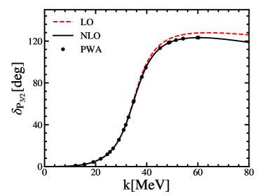
Figure 1: The $P_{3/2}$ phase shifts of $n\alpha$ scattering as a function of $k$. “PWA” refer to the phase shift analysis from Ref. Arndt et al. (1973).

IV Three-body system of neutron-neutron-$\alpha$

If the two-body system is the only application, developing an EFT to reproduce the well-known ERE seems an overkill. Nuclear EFTs often find their usefulness when more particles are present, e.g., a photon or other nucleons. Having built the EFT potentials for $n\alpha$, we apply its LO term in this section to the three-body system of $nn\alpha$ Rotureau and van Kolck (2013); Ji et al. (2014); Ryberg et al. (2017). This application is part of the research program of so-called halo/cluster EFTs (see Refs. van Kolck (2005b); Hammer et al. (2017); Ando (2021); Hammer et al. (2020) for reviews).

The $nn\alpha$ system is interesting in its own right. In this three-body system, none of the two-body subsystems are bound but $nn\alpha$ together can form the stable isotope of ⁶He, an instance of so-called Borromean states. The $n\alpha$ interaction supports a narrow $P$-wave resonance but not a bound state, and the $nn$ pair is not known to be bound either, dictated instead by a shallow $S$-wave virtual state. However, the three-body system is bound by 0.969 MeV, known as the ground state of ⁶He.

We follow mostly the computational framework of Refs. Ji et al. (2014); Hammer et al. (2017), with the only difference being the form of $n\alpha$ interaction. Some of the technicalities will be reviewed briefly. In addition to Eq. (3), we need Lagrangian terms to describe $nn$ interaction and, especially, the short-range three-body force that couples a neutron spectator to the $n\alpha$ pair in the $P$ wave:

$$\mathcal{L}_{nn} =-C_{\phi n}\left(\phi^{\dagger}n_{\delta}S^{\delta}n_{-\delta}+\mathrm{H.c.}\right)+\sigma\phi^{\dagger}\phi\,,$$ (44)

$$\mathcal{L}_{nn\alpha} =-h\left(G_{0}^{ab}T_{a}^{is}\Psi_{b}\overleftrightarrow{\partial_{i}}n_{s}\right)^{\dagger}\left(G_{0}^{cd}T_{c}^{jr}\Psi_{d}\overleftrightarrow{\partial_{j}}n_{r}\right)\,.$$ (45)

where $\phi$ is the ${{}^{1}\!{S}_{0}}$ $nn$ dibaryon field, and $S^{\delta}\equiv\langle 0,0|1/2,\delta;1/2,-\delta\rangle$ and $G_{0}^{ab}\equiv\langle 0,0|3/2,a;3/2,b\rangle$ are the Clebsch-Gordan coefficients and dummy indices are assumed to be summed up. With $m_{n}$ ($m_{\Psi}$) the mass of the neutron ($n\alpha$ resonance) Hammer et al. (2017), $\overleftrightarrow{\partial_{i}}\equiv[(m_{n}\overleftarrow{\nabla}-m_{\Psi}\overrightarrow{\nabla})/(m_{n}+m_{\Psi})]_{i}$ is the Galilean invariant derivative.

The three-body equation for the ⁶He bound state can be described diagrammatically in Fig. 2, where the two Faddeev components $F_{\alpha}$ and $F_{n}$ are defined according to which of $n$ and $\alpha$ is the spectator in Jacobi coordinates Ji et al. (2014); Hammer et al. (2017). The spin-parity $0^{+}$ state of the entire three-body system is considered, while at LO the $nn$ pair interacts in ${{}^{1}\!{S}_{0}}$ and the $n\alpha$ pair in the ${}^{2}P_{3/2}$ resonant channel. $F_{\alpha}$ and $F_{n}$ are defined such that the relative Jacobian angular momentum between the spectator particle and the pair is projected onto the $S$ wave between $\alpha$ and the $nn$ pair, and onto the $P$ wave between $n$ and the $n\alpha$ pair.

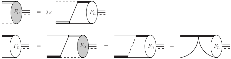
Figure 2: Diagrammatic representation for the coupled-channel $nn\alpha$ Faddeev equations. The single dashed and solid lines refer, respectively, to the $\alpha$ and neutron field. The grey and dark thick lines represent respectively the $nn$ and $n\alpha$ dimeron fields, $\phi$ and $\Psi$.

We use the second diagram of the second line in Fig. 2 to explain the kinematics. As a rule, the spectator external line is always chosen to be on-shell. Therefore, the neutron external line carries on-shell four-momentum $(q^{2}/2m_{n},\vec{q}\,)$, and the $\Psi$ external line for the $n\alpha$ pair has off-shell four-momentum $(-B_{3}-q^{2}/2m_{n},-\vec{q}\,)$ so that the three-body total energy is $-B_{3}$. After the $n\alpha$ pair exchanging a neutron with the spectator neutron, the remaining $\alpha$ carries a final four-momentum of $(q_{0}^{\prime},\vec{q}\,^{\prime})$, while the emerging $nn$ pair has $(-B_{3}-q_{0}^{\prime},-\vec{q}\,^{\prime})$. In addition, the $n\alpha$ pair carries a relative momentum between its constituents:

$$\vec{\pi}_{1}=\frac{4}{5}\vec{q}+\vec{q}\,^{\prime}\,.$$ (46)

We integrate out $q_{0}^{\prime}$ by picking the pole of the $\alpha$ propagator, which is consistent with the aforementioned rule of making the external spectator on-shell. The resulting integrals can be further decomposed by expanding with the Legendre polynomials in $\hat{q}\cdot\hat{q}^{\prime}$.

There are several key elements in assembling the coupled-channel integral equations, including the kernel functions and the dressed $nn$ and $n\alpha$ dimeron propagators. The kernel functions are the propagators of the exchanged particles multiplied by appropriate vertices. The one corresponding to the exchanged neutron combined with the $\phi nn$ and $n\alpha\Psi$ vertices, shown in the second diagram of the second line in Fig. 2, is given by

$$X_{n\alpha}(q,q^{\prime};B_{3})=\sqrt{2}\left[\frac{4}{5}q\,G_{n\alpha,0}(q,q^{\prime};B_{3})+q^{\prime}\,G_{n\alpha,1}(q,q^{\prime};B_{3})\right]\,,$$ (47)

where the angle-averaged Green’s function $G_{n\alpha,l}$ is projected onto the orbital quantum number $l$ by the Legendre polynomial $P_{l}$:

$$\begin{split}G_{n\alpha,l}(q,q^{\prime};B_{3})=\frac{m_{n}}{2}\int_{-1}^{1}d(\hat{q}\cdot\hat{q}^{\prime})\frac{P_{l}(\hat{q}\cdot\hat{q}^{\prime})}{\sqrt{\pi_{1}^{2}+\gamma^{2}}\left(m_{n}B_{3}+\frac{5}{8}\pi_{1}^{2}+\frac{3}{5}q^{2}\right)}\,.\end{split}$$ (48)

The kernel function for the second diagram of the first line in Fig. 2 is similar to $X_{n\alpha}(q,q^{\prime};B_{3})$, except for a simple adjustment of switching $q$ and $q^{\prime}$. The kernel function for the exchanged $\alpha$ in the third diagram of the second line is given by

$$X_{nn}(q,q^{\prime};B_{3}) = \frac{27}{25}qq^{\prime}\,G_{nn,0}(q,q^{\prime};B_{3})$$ (49)

$$\;+\frac{2}{5}(q^{2}+q^{\prime 2})\,G_{nn,1}(q,q^{\prime};B_{3})+qq^{\prime}\,G_{nn,2}(q,q^{\prime};B_{3}),$$

where

$$G_{nn,l}(q,q^{\prime};B_{3})=\frac{m_{n}}{2}\int_{-1}^{1}d(\hat{q}\cdot\hat{q}^{\prime})\frac{P_{l}(\hat{q}\cdot\hat{q}^{\prime})}{\sqrt{\pi_{2}^{2}+\gamma^{2}}\left(m_{n}B_{3}+\frac{5}{8}\pi_{2}^{2}+\frac{3}{5}q^{2}\right)\sqrt{\pi_{3}^{2}+\gamma^{2}}}\,,$$ (50)

with

$$\vec{\pi}_{2} = \frac{1}{5}\vec{q}+\vec{q}\,^{\prime}\,,$$

$$\vec{\pi}_{3} = \vec{q}+\frac{1}{5}\vec{q}\,^{\prime}\,.$$ (51)

For more detailed explanation concerning, for instance, the angular-momentum recoupling coefficients, we refer to Ref. Ji et al. (2014).

The $nn$ interaction is subsumed in the dressed ${{}^{1}\!{S}_{0}}$ dibaryon propagator, depicted by the grey lines, that depends only on the ${{}^{1}\!{S}_{0}}$ scattering length $a_{0}=-18.6$ fm at LO:

$$D_{nn}(\kappa)=-\frac{1}{2\pi^{2}m_{n}}\frac{1}{\kappa-a_{0}^{-1}}\,,$$ (52)

where $\kappa$ is related to the dibaryon four-momentum $(p_{0},\vec{p}\,)$ through $\kappa\equiv\sqrt{-m_{n}p_{0}+\vec{p}\,^{2}-i0}$. The ${{}^{1}\!{S}_{0}}$ $nn$ scattering amplitude can be written with $D_{nn}$ as

$$f_{nn}(k)=\frac{1}{k\cot\delta_{S}-ik}=-2\pi^{2}m_{n}D_{nn}(-ik)\,,$$ (53)

where $k$ is the c.m. momentum.

The dressed $\Psi$ propagator packs the two-body $P_{3/2}$ interaction of $n\alpha$:

$$D_{n\alpha}(\kappa)=-\frac{5}{16\pi^{2}m_{n}}\frac{\kappa+\gamma}{\kappa^{2}+\eta\kappa+\eta\gamma}\,,$$ (54)

where $\kappa\equiv\frac{2}{5}\sqrt{-10m_{n}p_{0}+\vec{p}\,^{2}-i0}$. The $P_{3/2}$ partial-wave amplitude of $n\alpha$ scattering is expressed in terms of $D_{n\alpha}$:

$$f_{n\alpha}(k)=\frac{1}{k\cot\delta_{P}-ik}=-\frac{16}{5}\frac{\pi^{2}m_{n}\eta}{\gamma-ik}D_{n\alpha}(-ik)\,.$$ (55)

With these ingredients, the coupled-channel integral equations for $F_{\alpha}(q)$ and $F_{n}(q)$ are established as follows:

$$F_{\alpha}(q) = 8\pi\int^{\Lambda_{3}}_{0}q^{\prime 2}dq^{\prime}\,X_{n\alpha}(q^{\prime},q;B_{3})\,D_{n\alpha}(\kappa_{1})\,F_{n}(q^{\prime})\,,$$ (56)

$$F_{n}(q) = 4\pi\int^{\Lambda_{3}}_{0}q^{\prime 2}dq^{\prime}\,X_{n\alpha}(q,q^{\prime};B_{3})\,D_{nn}(\kappa_{0})\,F_{\alpha}(q^{\prime})$$ (57)

$$+4\pi\int^{\Lambda_{3}}_{0}q^{\prime 2}dq^{\prime}\,\left[X_{nn}(q,q^{\prime};B_{3})+\frac{qq^{\prime}}{\Lambda_{3}^{4}}{H_{0}}(\Lambda_{3})\right]\,D_{n\alpha}(\kappa_{1})\,F_{n}(q^{\prime})~{},$$

where the $nn\alpha$ coupling $H_{0}(\Lambda_{3})\equiv h\Lambda_{3}^{4}$ and the c.m. momenta for the dimeron propagators are related to $B_{3}$ and $q^{\prime}$ as

$$\kappa_{0} \equiv \sqrt{m_{n}B_{3}+\frac{3}{8}{q^{\prime}}^{2}}\,,$$ (58)

$$\kappa_{1} \equiv \frac{2}{5}\sqrt{10m_{n}B_{3}+6{q^{\prime}}^{2}}\,.$$ (59)

For simplicity, we regularize the Jacobi momentum $q^{\prime}$ by an ultraviolet sharp cutoff $\Lambda_{3}$, while taking the cutoff values in the two-body interactions to infinities.

We begin by solving the three-body equations without the three-body force. More specifically, we calculate the binding energies of the $nn\alpha$ system $B_{3}$ as a function of $\Lambda_{3}$ while setting the three-body force parameter $H_{0}(\Lambda_{3})=0$. In the upper panel in Fig. 3, $B_{3}$ indicates a power-law dependence on $\Lambda_{3}$ when $\Lambda_{3}$ is much larger than $1/|a_{0}|$, $|k_{\pm}|$, and $\sqrt{m_{n}B_{3}}$. Meanwhile, a series of new bound states emerge as $\Lambda_{3}$ increases, and their binding energies form approximately a geometric series. These behaviors suggest that the Thomas collapse can also exist in three-body systems involving $P$-wave pairwise interactions.

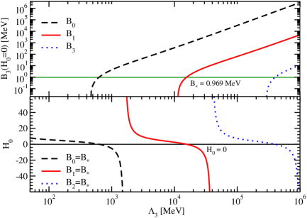
Figure 3: (Color online) Upper panel: The three-body binding energies as functions of the cutoff $\Lambda_{3}$ with $H_{0}=0$. The green solid line indicates the physical binding energy $B_{*}$. Lower panel: ${H_{0}}$ as a function of the cutoff $\Lambda_{3}$. The black solid line indicates the zero axis for $H_{0}=0$.

Therefore, it is essential to have the $nn\alpha$ three-body interaction at LO, in order to eliminate the cutoff dependence, in the meantime preventing the Thomas collapse. By tuning $H_{0}$ for any given values of $\Lambda_{3}$, the three-body binding energy is fitted to the experimental value of ⁶He binding energy $B_{*}=0.969$ MeV. In the lower panel in Fig. 3, $H_{0}$ displays logarithmic oscillatory dependence on $\Lambda_{3}$, similar to the system dominated by two-body $S$-wave interactions Bedaque et al. (1999). However, the logarithmic period of ${H}_{0}(\Lambda_{3})$ is no longer a constant. This is because the symmetry of discrete scale invariance, which is observed in $S$-wave three-body systems, is broken by the presence of $\gamma$, an important element in the LO $n\alpha$ potential to form the $P$-wave resonance.

For lowest cutoff values where there is only one bound state, fitting to $B_{*}$ is straightforward. As $\Lambda_{3}$ increases, $H_{0}$ decreases to negative values and eventually diverges at $\Lambda_{3}\approx 1.6$ GeV for the first time, where we begin instead to fit the first excited three-body state $B_{1}$ to $B_{*}$, resulting in emergence of a new $H_{0}$ branch from positive infinity. That is, the ground state is left to become an unphysical spurious state in the EFT. When $B_{1}$ is fixed, the ground-sate energy $B_{0}$ stays above 800 MeV, which is far beyond the EFT breakdown scale. Similar discontinuity of $H_{0}(\Lambda_{3})$ is also shown at $\Lambda_{3}\approx 40$ GeV, when $B_{1}$ becomes too large to reproduce $B_{*}$, and the second excited state is used to reproduce the physical ⁶He state.

After the three-body energy is renormalized, the Faddeev components $F_{n}(q)$ and $F_{\alpha}(q)$ are calculated and checked for their cutoff dependence. In Fig. 4, the Faddeev components $F_{n}$ and $F_{\alpha}$ are plotted as functions of the Jacobi momentum $q$ for a set of cutoff values. The low-momentum part of both Faddeev components exhibits an insignificant cutoff variation for $\Lambda_{3}\geqslant 300$ MeV, which suggests that the structure properties of ⁶He will be cutoff invariant at LO.

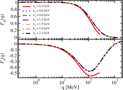
Figure 4: (Color online) The Faddeev components $F_{\alpha}$ and $F_{n}$ as functions of $q$, calculated with $\Lambda_{3}=$ 0.3 GeV (red solid line), 0.6 GeV (blue dotted line), 0.9 GeV (green dash-dotted line), 1.2 GeV (purple long-dashed line), 1.5 GeV (orange dot-dashed line), 1.8 GeV (brown dot-dashed line), and 2.1 GeV (black dot-dashed line). The Faddeev components are normalized to $F_{\alpha}(0)=1$.

We have shown that the nonlocal, momentum-dependent $n\alpha$ interaction (2) can produce the same qualitative features of the $nn\alpha$ three-body system as those in Refs. Rotureau and van Kolck (2013); Ji et al. (2014) using an energy-dependent $n\alpha$ potential. The most important one is that the $nn\alpha$ three-body force must appear at LO. By replacing the energy-dependent $n\alpha$ potential with the momentum-dependent one, we can retain the fully unitary form of the $n\alpha$ dimeron propagator $D_{n\alpha}$, and in the meantime, without worrying about the unphysical redundant pole.

V Summary and outlook

Inspired by previous works for $S$-wave interactions, we have used a momentum-dependent nonlocal potential (2) to develop an EFT for shallow $P$-wave resonances. The goal is to construct a framework more suitable, at least for some many-body methods, to apply in many-body calculations than previous implementations based on energy-dependent potentials.

We have shown that the potential generates the effective-range expansion with the scattering volume and generalized effective range term as the LO. Although the LO $S$ matrix has a third pole besides the resonance poles, it does not correspond to a negative-norm bound state unlike in the case of energy-dependent potentials. Higher-order ERE terms can be attained by adding systematically higher-order potentials in perturbation theory. Despite their ultraviolet (UV) suppression the potentials still need regularization, and renormalization was explained up to N²LO for the two-body sector. Subleading potentials resemble those $S$-wave potentials proposed in Ref. Beane and Farrell (2022), although the UV/IR symmetry of the $S$-matrix seems to be lost.

We then applied the framework to the neutron-$\alpha$ system where the $P_{3/2}$ resonance is a prominent feature. The same scaling for the ERE parameters as in Ref. Bertulani et al. (2002) was assumed, but our framework does not generate the deep bound state as that of Ref. Bertulani et al. (2002) would. In addition, the correspondence between the Lagrangian parameters is, not surprisingly, obscured by distinctive forms of the interactions. The NLO phase shifts showed excellent agreement with the phase shift analysis from Ref. Arndt et al. (1973).

The neutron-neutron-$\alpha$ system was studied, with the intention to examine whether the three-body physics learned in Ref. Ji et al. (2014) can be recovered with the nonlocal potential. The answer is affirmative. The three-body force is confirmed to be at LO on renormalization ground. With the three-body parameter $H_{0}$ fitted to the ⁶He binding energy, the running of $H_{0}(\Lambda)$ also shows a limit-cycle behavior. However, the advantage of the momentum-dependent $n$-$\alpha$ interaction will only be fully realized in still higher-body calculations where it becomes increasingly difficult to implement energy-dependent potentials. This is under investigation.