General exponential basis set parametrization: Application to time-dependent bivariational wave functions

Abstract

We present eom for general time-dependent wave functions with exponentially parametrized biorthogonal basis sets. The equations are fully bivariational in the sense of the tdbvp and offer an alternative, constraint free formulation of adaptive basis sets for bivariational wave functions. We simplify the highly non-linear basis set equations using Lie algebraic techniques and show that the computationally intensive parts of the theory are in fact identical to those that arise with linearly parametrized basis sets. Our approach thus offers easy implementation on top of existing code in the context of both nuclear dynamics and time-dependent electronic structure. Computationally tractable working equations are provided for single and double exponential parametrizations of the basis set evolution. The eom are generally applicable for any value of the basis set parameters, unlike the approach of transforming the parameters to zero at each evaluation of the eom. We show that the basis set equations contain a well-defined set of singularities, which are identified and removed by a simple scheme. The exponential basis set equations are implemented in conjunction with tdmvcc and we investigate the propagation properties in terms of the average integrator step size. For the systems we test, the exponentially parametrized basis sets yield slightly larger step sizes compared to linearly parametrized basis set.

I Introduction

Optimized basis sets are ubiquitous in time-independent quantum chemistry, since the proper choice of basis is crucial to a compact representation of the wave function. The paradigmatic example in electronic structure theory is the scf method, while vibrational scf (vscf) plays a similar role in vibrational structure theory. Correlated electronic wave function methods that simultaneously optimize the basis set are also in widespread use, with multi-configurational scf (mcscf) as the standard example and dmrg with self-consistently optimized orbitals (DMRG-SCF)Zgid and Nooijen (2008); Ghosh et al. (2008); Ma et al. (2017) as a more recent example. Basis set optimization also plays a role in electronic cc theory through orthogonalSherrill et al. (1998); Pedersen, Koch, and Hättig (1999) and non-orthogonalPedersen, Fernández, and Koch (2001) orbital-optimized coupled cluster (occ and nocc). These and similar methods require special formal considerations since they are not variational (in the sense of providing an upper bound on the energy) and since the bra and ket states are parametrized in an asymmetric fashion. A principled way of handling this asymmetry while ensuring convergence to fci is to use the bivariational framework pioneered by ArponenArponen (1983). The nocc method is fully bivariational and thus convergesMyhre (2018) to fci, while occ does notKöhn and Olsen (2005).

Optimized or adaptive basis sets are also important in explicitly time-dependent theory as illustrated by the success of methods such as mctdhMeyer, Manthe, and Cederbaum (1990); Beck et al. (2000) for nuclear dynamics and the related mctdhfZanghellini et al. (2003); Caillat et al. (2005) for electronic dynamics. Various schemes that use adaptive basis sets (like mctdh and mctdhf) but restrict or truncate the wave function expansion are known as well. Kato and Kono (2004); Sato and Ishikawa (2013); Miyagi and Madsen (2013); Haxton and McCurdy (2015); Sato and Ishikawa (2015); Worth (2000); Wodraszka and Carrington (2016); Larsson and Tannor (2017); Madsen et al. (2020a, b) Methods that treat mixed particle types (e.g. fermionic and bosonic) also exist. Alon, Streltsov, and Cederbaum (2007, 2008); Nest (2009); Manthe and Weike (2017)

There has been considerable interest in formulating theories that combine the idea of adaptive basis sets with the use of asymmetric parametrizations such as coupled cluster. Although such theories can be quite involved, several works have appeared in the context of electronicKvaal (2012); Sato et al. (2018); Pedersen and Kvaal (2019); Kristiansen et al. (2020); Pathak, Sato, and Ishikawa (2020, 2021); Kristiansen et al. (2022) and nuclearMadsen et al. (2020c); Højlund et al. (2022) dynamics. Some of these works (as well as the present work) utilize Arponen’s tdbvpArponen (1983), which offers a clear formal strategy for deriving eom. However, additional work is typically needed to obtain the eom in a computationally tractable format and to analyze the eom for redundancies and singularities.

It is well known that unitary (invertible) basis set transformations can be parametrized in terms of the exponential of an anti-Hermitian (general) one-particle operator $\hat{\kappa}$ (see Ref. 37 for an overview of the standard mathematical machinery). This constraint free approach results in simple equations when expanding around $\hat{\kappa}=0$ and has been used frequently in the context of time-independent theory and response theory where one can trivially obtain $\hat{\kappa}=0$ by absorbing a non-zero $\hat{\kappa}$ into the Hamiltonian integrals. In an explicitly time-dependent context the situation is more complicated and a linear parametrization with constraints has usually been preferred over the exponential parametrization. However, a few exceptions can be found in the literature: Pedersen and KochPedersen and Koch (1998) presented general considerations on exponentially parametrized tdhf but did not derive explicit eom for $\hat{\kappa}$. Madsen et al.Madsen et al. (2018) derived and implemented the eom for xtdh without assuming $\hat{\kappa}=0$. In this case the exponential parametrization resulted in substantial computational gains compared to the conventional linear parametrization. Recently, Kristiansen et al.Kristiansen et al. (2022) considered time-dependent occ and nocc with double excitations (TDOCCD and TDNOCCD) and introduced the corresponding second-order approximations TDOMP2 and TDNOMP2 with exponentially parametrized orbitals. They used the $\hat{\kappa}=0$ method to simplify derivations while keeping the benefit of a contraint free formulation. We note that the exponential parametrization with $\hat{\kappa}=0$ and the linear parametrization with constraints result in very similar working equations although the derivations have different starting points. Allowing $\hat{\kappa}\neq 0$ leads to substantially different equations.

The question of how to parametrize basis sets is not only one of mathematical convenience— it also plays an important role in the propagation of time-dependent wave functions. This inludes questions of numerical stability and integrator step size, the latter being a determining factor of the computational cost.

In a recent paperHøjlund et al. (2022) we considered linear basis set parametrization and a novel parametrization based on polar decomposition for general time-dependent bivariational wave functions. The purpose of that work was mainly to study the effect on the numerical stability of tdmvccMadsen et al. (2020c) and it was shown that a so-called restricted polar parametrization offered improved numerical stability compared to the linear parametrization. The present work considers the eom for similar kinds of wave functions with exponentially parametrized basis sets without assuming $\hat{\kappa}=0$. In addition to the single exponential formalism, we also consider a double exponential basis set parametrization. The former corresponds to the linear parametrization, while the latter parallels the polar parametrization of Ref. 36. The eom derived are general with respect to the type of wave function expansion but the main application is cc theory where a bivariational formulation is natural. We note that the derivations are mainly presented in the language and notation of vibrational structure theory but that all theoretical results carry over to electronic structure theory after minor notational adjustments such as dropping mode indices and sums over modes.

The paper is organized as follows: Section II covers the theory, including a brief introduction to the tdbvp and derivations of eom. This is followed by a description of our implementation for the nuclear dynamics case in Sec. III and a few numerical examples in Sec. IV. Section V concludes the paper with a summary of our findings and an outlook on future work.

II Theory

II.1 The time-dependent bivariational principle

Following ArponenArponen (1983), we consider a general bivariational Lagrangian,

$$\mathcal{L}=\langle\Psi^{\prime}|(i\partial_{t}-H)|\Psi\rangle,$$ (1)

where the bra and ket states are independent. We then determine stationary points ($\delta\mathcal{S}=0$) of the action-like functional

$$\mathcal{S}=\int_{t_{0}}^{t_{1}}\mathcal{L}\differential{t}$$ (2)

under the condition that the variations of the bra and ket vanish at the endpoints of the integral. In the exact-theory case, a short calculation shows that this procedure is equivalent to the tdse and its complex conjugate. For approximate, parametrized wave functions, the stationarity condition is instead equivalent to a set of ele,

$$0=\partialderivative{\mathcal{L}}{y_{i}}-\derivative{t}\partialderivative{\mathcal{L}}{\dot{y}_{i}},$$ (3)

for all parameters $y_{i}$ (a short proof of this well-known fact is given in Ref. 36 in a notation consistent with the present work). Writing the Lagrangian as

$$\mathcal{L}=\mathcal{I}-\mathcal{H}$$ (4)

with

$$\mathcal{I}(\mathbf{y},\dot{\mathbf{y}})=i\braket{\Psi^{\prime}}{\dot{\Psi}}=i\sum_{j}\dot{y}_{j}\Big{\langle}\Psi^{\prime}\mspace{2.0mu}\Big{|}\mspace{1.5mu}\partialderivative{\Psi}{y}\Big{\rangle},$$ (5a)

$$\mathcal{H}(\mathbf{y},t)=\langle\Psi^{\prime}|H|\Psi\rangle,$$ (5b)

the ele in Eq. (3) become

$$\partialderivative{\mathcal{I}}{y_{i}}-\derivative{t}\partialderivative{\mathcal{I}}{\dot{y}_{i}}=\partialderivative{\mathcal{H}}{y_{i}}.$$ (6)

After carrying out the derivatives using the chain and product rules and cancelling terms, one gets the following appealing eom:

$$i\sum_{j}\mathcal{M}_{ij}\dot{y}_{j} =\partialderivative{\mathcal{H}}{y_{i}}.$$ (7)

Here, we have defined an anti-symmetric matrix $\bm{\mathcal{M}}$ with elements

$$\mathcal{M}_{ij}=\Big{\langle}\partialderivative{\Psi^{\prime}}{y_{i}}\mspace{2.0mu}\Big{|}\mspace{1.5mu}\partialderivative{\Psi}{y_{j}}\Big{\rangle}-\Big{\langle}\partialderivative{\Psi^{\prime}}{y_{j}}\mspace{2.0mu}\Big{|}\mspace{1.5mu}\partialderivative{\Psi}{y_{i}}\Big{\rangle}.$$ (8)

The eom in Eq. (7) consititute a natural bivariational analogue of the general variational eom considered by e.g. Kramer and SaracenoKramer and Saraceno (1981) and OhtaOhta (2004).

II.2 Parametrization

We will consider general wave function parametrizations of the form

$$\ket{\Psi(\bm{\alpha},\bm{\kappa})} =e^{\hat{\kappa}}\ket{\psi(\bm{\alpha})}$$ (9a)

$$\bra{\Psi^{\prime}(\bm{\alpha},\bm{\kappa})} =\bra{\psi^{\prime}(\bm{\alpha})}e^{-\hat{\kappa}}$$ (9b)

where the one-particle operator $\hat{\kappa}$ generates invertible linear transformations of the basis functions (modals or orbitals). In the vibrational case, we use the notation of many-mode second quantizationChristiansen (2004) and write

$$\hat{\kappa}=\sum_{m}\sum_{p^{m}q^{m}}\kappa^{m}_{{p}^{m}{q}^{m}}E^{m}_{{p}^{m}{q}^{m}}.$$ (10)

The parameters $\kappa^{m}_{{p}^{m}{q}^{m}}$ are collected in vectors $\bm{\kappa}^{m}$ or matrices $\mathbf{K}^{m}$ depending on context. The one-mode shift operators,

$$E^{m}_{{p}^{m}{q}^{m}}=a^{m\mspace{-0.5mu}\raisebox{0.90417pt}{$\scriptstyle\dagger$}}_{\mspace{0.0mu}p^{m}}b^{m}_{\mspace{-1.0mu}q^{m}},$$ (11)

satisfy the commutator

$$[E^{m}_{{p}^{m}{q}^{m}},E^{m^{\prime}}_{{r}^{m^{\smash{\prime}}}\!{s}^{m^{\smash{\prime}}}}]=\delta_{mm^{\prime}}(\delta_{q^{m}r^{m}}E^{m}_{{p}^{m}{s}^{m}}-\delta_{p^{m}s^{m}}E^{m}_{{r}^{m}{q}^{m}})$$ (12)

and constitute the generators of the general linear group. The well-known one-electron shift operators satisfy essentially the same commutatorHelgaker, Jørgensen, and Olsen (2000), which means that the derivations in this work carry over to electronic structure theory after removing mode indices as appropriate. We will denote the remaining wave function parameters $\bm{\alpha}$ as configurational parameters. The non-transformed states $\ket{\psi(\bm{\alpha})}$ and $\bra{\psi^{\prime}(\bm{\alpha})}$ are assumed to be expressed in the same primitive basis as the $\hat{\kappa}$ operator. We will allow for the case where the wave function is expanded in an active subset of the primitive basis. In Sec. II.3 we simply require that the primitive basis is biorthonormal, while we require orthonormality in Sec. II.6. We note that this restriction can likely be lifted with appropriate modifications of the derivations.

II.3 Equations of motion

Ordering the parameters like $\mathbf{y}=(\bm{\alpha},\bm{\kappa})$, the eom in Eq. (7) assume the structure

$$i\left[\begin{array}[]{c | c}\mathbf{M}&{\mspace{8.0mu}\tilde{\mathbf{A}}\mspace{5.0mu}}\\ \hline\cr-\tilde{\mathbf{A}}^{\mspace{-2.0mu}\mspace{-3.0mu}\mathsf{T}}&{\mspace{8.0mu}\tilde{\mathbf{C}}\mspace{5.0mu}}\end{array}\right]\left[\begin{array}[]{c}\dot{\bm{\alpha}}\\ \hline\cr\dot{\bm{\kappa}}\end{array}\right]=\left[\begin{array}[]{c}\mathbf{h}\\ \hline\cr\tilde{\mathbf{f}}\end{array}\right].$$ (19)

The various matrix elements can be calculated by direct application of Eq. (8) followed by the appropriate use of

$$e^{\hat{\kappa}}e^{-\hat{\kappa}} =1,$$ (20a)

$$\partialderivative{e^{-\hat{\kappa}}}{\kappa^{m}_{{p}^{m}{q}^{m}}}e^{\hat{\kappa}} =-e^{-\hat{\kappa}}\partialderivative{e^{\hat{\kappa}}}{\kappa^{m}_{{p}^{m}{q}^{m}}}$$ (20b)

where the latter follows from taking the derivative of the former. For notational convenience, we define a similarity transformed derivativeHall (2015); Olsen and Jørgensen (1985)

$$D^{m}_{{p}^{m}{q}^{m}} =e^{-\hat{\kappa}}\partialderivative{e^{\hat{\kappa}}}{\kappa^{m}_{{p}^{m}{q}^{m}}}$$

$$=e^{-\hat{\kappa}^{m}}\partialderivative{e^{\hat{\kappa}^{m}}}{\kappa^{m}_{{p}^{m}{q}^{m}}}$$

$$=\sum_{n=0}^{\infty}\frac{(-1)^{n}}{(n+1)!}(\mathrm{ad}_{\hat{\kappa}^{m}})^{n}E^{m}_{{p}^{m}{q}^{m}}$$

$$=\sum_{r^{m}s^{m}}d^{m}_{({p}^{m}{q}^{m})({r}^{m}{s}^{m})}E^{m}_{{r}^{m}{s}^{m}}$$ (21)

with $\mathrm{ad}_{\hat{\kappa}^{m}}(X)=[\hat{\kappa}^{m},X]$ (the second equality follows from the fact that $[\hat{\kappa}^{m},\hat{\kappa}^{m^{\prime}}]=0$ for $m\neq m^{\prime}$). This operator is a one-particle operator as indicated by the last equality in Eq. (II.3). For now we assume that the matrix elements $d^{m}_{({p}^{m}{q}^{m})({r}^{m}{s}^{m})}$ are available and collect them in a matrix $\mathbf{D}^{m}$. We will later show how the elements of $\mathbf{D}^{m}$ can be calculated and, in particular, how transformations by $\mathbf{D}^{m}$ can be performed in an efficient manner without explicitly constructing the full matrix. The matrix elements needed for Eq. (19) are now given by

$$M_{ij} =\Big{\langle}\partialderivative{\psi^{\prime}}{\alpha_{i}}\mspace{2.0mu}\Big{|}\mspace{1.5mu}\partialderivative{\psi}{\alpha_{j}}\Big{\rangle}-\Big{\langle}\partialderivative{\psi^{\prime}}{\alpha_{j}}\mspace{2.0mu}\Big{|}\mspace{1.5mu}\partialderivative{\psi}{\alpha_{i}}\Big{\rangle}$$ (22a)

$$\tilde{A}_{{i}({m^{\prime}}{r}^{m^{\smash{\prime}}}\!{s}^{m^{\smash{\prime}}})} =\partialderivative{\alpha_{i}}\langle\psi^{\prime}|D^{m^{\prime}}_{{r}^{m^{\smash{\prime}}}\!{s}^{m^{\smash{\prime}}}}|\psi\rangle$$ (22b)

$$\tilde{C}_{({m}\,{p}^{m}{q}^{m})({m^{\prime}}{r}^{m^{\smash{\prime}}}\!{s}^{m^{\smash{\prime}}})} =\langle\psi^{\prime}|[D^{m^{\prime}}_{{r}^{m^{\smash{\prime}}}\!{s}^{m^{\smash{\prime}}}},D^{m}_{{p}^{m}{q}^{m}}]|\psi\rangle$$ (22c)

$$h_{i} =\partialderivative{\alpha_{i}}\langle\psi^{\prime}|\bar{H}|\psi\rangle$$ (22d)

$$\tilde{f}_{(m\,{p}^{m}{q}^{m})} =\langle\psi^{\prime}|[\bar{H},D^{m}_{{p}^{m}{q}^{m}}]|\psi\rangle$$ (22e)

where we have defined

$$\bar{H}=e^{-\hat{\kappa}}He^{\hat{\kappa}}$$ (23)

and used a tilde to indicate the quantities that depend on the $D^{m}_{{p}^{m}{q}^{m}}$ operators. These quantities can be quite complicated since $D^{m}_{{p}^{m}{q}^{m}}$ is generally a full one-particle operator. In particular, one cannot immediately analyze the elements of $\tilde{\mathbf{A}}$ and $\tilde{\mathbf{C}}$ for zeros. Having calculated the matrix elements of the eom, it is easy to show that Eq. (19) is equivalent to

$$i\dot{\bm{\alpha}} =\mathbf{M}^{-1}\big{(}\mathbf{h}-i\tilde{\mathbf{A}}\dot{\bm{\kappa}}\big{)},$$ (24a)

$$i\big{(}\tilde{\mathbf{C}}+\tilde{\mathbf{A}}^{\mspace{-3.0mu}\mathsf{T}}\mathbf{M}^{-1}\tilde{\mathbf{A}}\big{)}\dot{\bm{\kappa}} =\tilde{\mathbf{f}}+\tilde{\mathbf{A}}^{\mspace{-3.0mu}\mathsf{T}}\mathbf{M}^{-1}\mathbf{h}.$$ (24b)

if $\mathbf{M}$ is invertible. The $\mathbf{M}$ matrix is usually rather trivial in a way that does not depend on the concrete parameter values but rather on the type of parametrization. Two examples (coupled cluster and linearly expanded wave functions) are given in Ref. 36. In those cases, the $\mathbf{M}$ matrix and its inverse are simply given by

$$\mathbf{M}=\left[\begin{array}[]{c | c}\mathbf{0}&-\mathbf{1}\\ \hline\cr+\mathbf{1}&\mathbf{0}\end{array}\right],\quad\mathbf{M}^{-1}=\left[\begin{array}[]{c | c}\mathbf{0}&+\mathbf{1}\\ \hline\cr-\mathbf{1}&\mathbf{0}\end{array}\right].$$ (29)

For extended coupled cluster, the $\mathbf{M}$ matrix is not trivial but it can still be inverted analytically and without singularities.Hansen, Madsen, and Christiansen (2020) We are currently not aware of any wave function where $\mathbf{M}$ can become singular. Instead, the main difficulty is that Eq. (24b) cannot generally (i.e. for $\hat{\kappa}\neq 0$) be solved as it stands due to the presence of redundancies that do not simply consist of certain blocks being equal to zero. We can circumvent this problem by introducing appropriate zeroth order quantities, i.e.

$$A_{{i}({m^{\prime}}{r}^{m^{\smash{\prime}}}\!{s}^{m^{\smash{\prime}}})} =\partialderivative{\alpha_{i}}\langle\psi^{\prime}|E^{m^{\prime}}_{{r}^{m^{\smash{\prime}}}\!{s}^{m^{\smash{\prime}}}}|\psi\rangle,$$ (30a)

$$C_{({m}\,{p}^{m}{q}^{m})({m^{\prime}}{r}^{m^{\smash{\prime}}}\!{s}^{m^{\smash{\prime}}})} =\langle\psi^{\prime}|[E^{m^{\prime}}_{{r}^{m^{\smash{\prime}}}\!{s}^{m^{\smash{\prime}}}},E^{m}_{{p}^{m}{q}^{m}}]|\psi\rangle,$$ (30b)

$$f_{(m\,{p}^{m}{q}^{m})} =\langle\psi^{\prime}|[\bar{H},E^{m}_{{p}^{m}{q}^{m}}]|\psi\rangle.$$ (30c)

These are simpler to calculate and, more importantly, allow a straight-forward (although possibly tedious) identification of vanishing matrix elements through analysis of the shift operator expressions. The introduction of a block-diagonal matrix $\mathbf{D}$ with elements

$$d_{({m}\,{p}^{m}{q}^{m})({m^{\prime}}{r}^{m^{\smash{\prime}}}\!{s}^{m^{\smash{\prime}}})}=\delta_{mm^{\prime}}d^{m}_{({p}^{m}{q}^{m})({r}^{m}{s}^{m})}$$ (31)

now allows us to write

$$\tilde{\mathbf{A}} =\mathbf{A}\mathbf{D}^{\mspace{-3.0mu}\mathsf{T}},$$ (32a)

$$\tilde{\mathbf{C}} =\mathbf{D}\mathbf{C}\mathbf{D}^{\mspace{-3.0mu}\mathsf{T}},$$ (32b)

$$\tilde{\mathbf{f}} =\mathbf{D}\mathbf{f},$$ (32c)

thus relating the simple zeroth order matrices to the infinite order matrices. Substituting Eqs. (32) into Eqs. (24) then yields

$$i\dot{\bm{\alpha}} =\mathbf{M}^{-1}\big{(}\mathbf{h}-i\mathbf{A}\mathbf{D}^{\mspace{-3.0mu}\mathsf{T}}\dot{\bm{\kappa}}\big{)},$$ (33a)

$$i\mathbf{D}\big{(}\mathbf{C}+\mathbf{A}^{\mspace{-3.0mu}\mathsf{T}}\mathbf{M}^{-1}\mathbf{A}\big{)}\mathbf{D}^{\mspace{-3.0mu}\mathsf{T}}\dot{\bm{\kappa}} =\mathbf{D}\big{(}\mathbf{f}+\mathbf{A}^{\mspace{-3.0mu}\mathsf{T}}\mathbf{M}^{-1}\mathbf{h}\big{)}.$$ (33b)

These equations are further simplified by removing $\mathbf{D}$ on both sides of Eq. (33b) and introducing the definition

$$\mathbf{g}=i\mathbf{D}^{\mspace{-3.0mu}\mathsf{T}}\dot{\bm{\kappa}}$$ (34)

in order to write

$$i\dot{\bm{\alpha}} =\mathbf{M}^{-1}\big{(}\mathbf{h}-\mathbf{A}\mathbf{g}\big{)},$$ (35a)

$$\big{(}\mathbf{C}+\mathbf{A}^{\mspace{-3.0mu}\mathsf{T}}\mathbf{M}^{-1}\mathbf{A}\big{)}\mathbf{g} =\big{(}\mathbf{f}+\mathbf{A}^{\mspace{-3.0mu}\mathsf{T}}\mathbf{M}^{-1}\mathbf{h}\big{)}.$$ (35b)

Equations (35) are the central equations of the present work and determine the time evolution of the parameters. Equation (35a) directly gives the time derivative of the configurational parameters, while Eq. (35b) determines the evolution of the basis set parameters in a slightly indirect way: First the equation is solved, and then $\dot{\bm{\kappa}}$ is recovered from Eq. (34). In the general case, this involves the inversion of $\mathbf{D}^{\mspace{-3.0mu}\mathsf{T}}$, while the computation reduces to $\dot{\bm{\kappa}}=-i\mathbf{g}$ in the $\hat{\kappa}=0$ case. It is interesting to note that Eqs. (35) are in fact identical to the central equations for bivariational wave functions with linearly parametrized basis sets [Eqs. (46) and (63) in Ref. 36]. It that work, Eq. (35b) appeared as a consequence of the necessary biorthonormality constraints and it was shown how it can be analyzed for redundancies and solved for relevant types of wave functions, e.g. cc. The important point here is that the central and computationally intensive equations are independent of the choice of basis set parametrization.

As a final simplification we define

$$\mathbf{h}^{\prime} =\mathbf{h}-\mathbf{A}\mathbf{g}$$ (36)

and write the configurational eom compactly as

$$i\dot{\bm{\alpha}} =\mathbf{M}^{-1}\mathbf{h}^{\prime}.$$ (37)

According to Eqs. (22d) and (30a) one may calculate the elements of $\mathbf{h}^{\prime}$ as

$$h_{i}^{\prime}=\partialderivative{\alpha_{i}}\langle\psi^{\prime}|(\bar{H}-\hat{g})|\psi\rangle=\partialderivative{\mathcal{H}^{\prime}}{\alpha_{i}}$$ (38)

with the one-particle operator $\hat{g}$ and the modified Hamiltonian function $\mathcal{H}^{\prime}$ given by

$$\hat{g} =\sum_{m}\sum_{p^{m}q^{m}}g^{m}_{{p}^{m}{q}^{m}}E^{m}_{{p}^{m}{q}^{m}},$$ (39)

$$\mathcal{H}^{\prime} =\langle\psi^{\prime}|(\bar{H}-\hat{g})|\psi\rangle.$$ (40)

Assuming that we are able to solve Eq. (35b) for $\mathbf{g}$, we need to recover $\dot{\bm{\kappa}}$ in order to integrate the eom. Using the definition in Eq. (34) and taking $\mathbf{D}^{\mspace{-3.0mu}\mathsf{T}}$ to be invertible, this means that we should compute

$$\dot{\bm{\kappa}}^{m}=-i(\mathbf{D}^{m})^{-\mspace{-3.0mu}\mathsf{T}}\mathbf{g}^{m}$$ (41)

for each mode. Doing this efficiently requires some general considerations on similarity transformed derivatives such as the one in Eq. (II.3). These considerations are covered by the next section.

II.4 Similarity transformed derivative

In this section, we leave the notation of the main text and consider a general Lie group. We note that the following derivations are rather generic in a Lie group context but we give the details for the convenience of the reader. Somewhat similar considerations (although considerably less general) can be found in Exercise 3.5 of Ref. 37.

The generators of the group (i.e. the basis of the Lie algebra) will be denoted by $E_{i}$ where $i$ might be a compound index. An element $X$ of the Lie algebra can then be written as

$$X=X_{i}E_{i}$$ (42)

where repeated indices imply summation (this convention is used throughout this section). The Lie algebra is characterized by the commutators (Lie brackets)

$$[E_{i},E_{j}]=f^{k}_{ij}E_{k}$$ (43)

where the scalars $f^{k}_{ij}$ are denoted structure constants. Equation (43) is completely general and covers, e.g., the one-particle shift operator commutator in Eq. (12). We will consider the case where $X$ depends on a parameter $s$ through the coefficients $X_{i}$ and compute the quantityHall (2015)

$$D=e^{-X(s)}\derivative{s}e^{X(s)}=\sum_{k=0}^{\infty}\frac{(-1)^{k}}{(k+1)!}(\mathrm{ad}_{X})^{k}\dot{X}$$ (44)

where

$$\mathrm{ad}_{X}(Y)=[X,Y],$$ (45)

$$\dot{X}=\derivative{X}{s}=\derivative{X_{i}}{s}E_{i}=\dot{X}_{i}E_{i}.$$ (46)

Before proceeding we note that

$$[X,E_{i}]=X_{j}[E_{j},E_{i}]=X_{j}f^{k}_{ji}E_{k}=Q_{ik}E_{k}$$ (47)

where we have defined a matrix $\mathbf{Q}$ with elements

$$Q_{ik}=X_{j}f^{k}_{ji}.$$ (48)

Equation (47) simply shows that commutation by $X$ translates to contraction with the matrix $\mathbf{Q}$. Using this fact, the first few commutators in the expansion become

$$(\mathrm{ad}_{X})^{0}\dot{X} =\dot{X}_{i}E_{i}$$

$$=\dot{X}_{i}(\mathbf{Q}^{0})_{ij}E_{j},$$ (49a)

$$(\mathrm{ad}_{X})^{1}\dot{X} =[X,\dot{X}_{i}E_{i}]$$

$$=\dot{X}_{i}(\mathbf{Q}^{1})_{ij}E_{j},$$ (49b)

$$(\mathrm{ad}_{X})^{2}\dot{X} =[X,[X,\dot{X}_{i}E_{i}]]$$

$$=\dot{X}_{i}(\mathbf{Q}^{2})_{ij}E_{j},$$ (49c)

$$\mathmakebox[\widthof{{}={}}][c]{\vdots}$$

Combining this pattern with Eq. (44) yields an attractive expression, namely

$$D=\dot{X}_{i}\Bigg{[}\sum_{k=0}^{\infty}\frac{(-1)^{k}}{(k+1)!}\mathbf{Q}^{k}\Bigg{]}_{ij}E_{j}\equiv\dot{X}_{i}d_{ij}E_{j}.$$ (50)

We collect the elements $d_{ij}$ in a matrix $\mathbf{D}$. This matrix encodes the structure of the Lie algebra (through the structure constants) and the information tied to the specific element $X$ and provides, in essence, a local basis for expressing $D$ directly in terms of the generators.

If we choose $s=X_{k}$, then it must be the case that $\dot{X}_{i}=\delta_{ki}$ and the equation above simplifies to

$$D=d_{kj}E_{j}$$ (51)

In this case, we see that the $\mathbf{D}$ matrix simply contains the expansion coefficients for the operator $D$. In order to compute $\mathbf{D}$, we assume that $\mathbf{Q}$ is diagonalizable as $\mathbf{Q}=\mathbf{P}\bm{\Lambda}\mathbf{P}^{-1}$ and write

$$\mathbf{D} =\mathbf{P}\varphi(\bm{\Lambda})\mathbf{P}^{-1}$$ (52)

where the function

$$\varphi(z) =\sum_{k=0}^{\infty}\frac{(-1)^{k}}{(k+1)!}z^{k}=\left\{\begin{array}[]{@{}c@{\quad}l@{}}\displaystyle\frac{1-\mathrm{exp}(-z)}{z}&\text{if }z\neq 0\\ 1&\text{if }z=0\end{array}\right.$$ (55)

is applied to the diagonal elements $\lambda_{i}$ of $\bm{\Lambda}$, i.e. to the eigenvalues of $\mathbf{Q}$. We have used the limit $\varphi(z)\rightarrow 1$ as $z\rightarrow 0$ to define $\varphi(0)$. Looking at Eq. (52) it is evident that $\mathbf{D}$ has eigenvalues $\varphi(\lambda_{i})$. This implies that $\mathbf{D}$ is invertible when $\varphi(\lambda_{i})\neq 0$, i.e. when $\lambda_{i}\neq 2\pi ik$ where $k$ is a non-zero integer.

II.5 Simplified equations of motion

Section II.4 provides a feasible and very general procedure for computing the $\mathbf{D}^{m}$ matrices. However, it is not at all obvious that this procedure will lead to efficient working equations. In Appendix A we work out the details and show that an attractive result can indeed be obtained provided the matrix $\mathbf{K}^{m}$ (which holds the elements of the vector $\bm{\kappa}^{m}$) is diagonalizable. Dropping the mode index for clarity, we assume that

$$\mathbf{K} =\mathbf{R}\bm{\mu}\mathbf{L}^{\dagger},\quad\mathbf{L}^{\dagger}\mathbf{R}=\mathbf{R}\mathbf{L}^{\dagger}=\mathbf{1}$$ (56)

where $\bm{\mu}$ is diagonal and construct an auxiliary matrix $\mathbf{\Omega}$ with elements

$$\omega_{pq}=1/\varphi(\mu_{p}-\mu_{q}).$$ (57)

The numbers $\varphi(\mu_{p}-\mu_{q})$ are in fact the eigenvalues of $\mathbf{D}^{\mspace{-3.0mu}\mathsf{T}}$ and our assumption that $\mathbf{D}^{\mspace{-3.0mu}\mathsf{T}}$ is invertible is equivalent to assuming

$$\varphi(\mu_{p}-\mu_{q})\neq 0\quad\Longleftrightarrow\quad\mu_{p}-\mu_{q}\neq 2\pi ik$$ (58)

where $k$ is a non-zero integer. With these prerequisites in place, the result is given by

$$\dot{\mathbf{K}}=-i\mathbf{R}\big{(}\mathbf{\Omega}\circ\big{(}\mathbf{L}^{\dagger}\mathbf{G}\mathbf{R}\big{)}\big{)}\mathbf{L}^{\dagger}$$ (59)

where $\dot{\mathbf{K}}$ and $\mathbf{G}$ are the matrices holding the elements of the vectors $\dot{\bm{\kappa}}$ and $\mathbf{g}$, respectively, for each mode (see Appendix A for details). The symbol $\circ$ denotes the Hadamard (or element-wise) product. Although the transformation in Eq. (59) may look somewhat unusual, it is not expensive to perform and can be easily implemented.

In summary, the steps necessary for the exponential parametrization are as follows: (i) solve Eq. (35b) to obtain $\mathbf{G}$; (ii) diagonalize $\mathbf{K}$ as in Eq. (56); (iii) compute $\mathbf{\Omega}$ using Eq. (57); and (iv) obtain $\dot{\mathbf{K}}$ from Eq. (59). Regarding the computational cost, we note that the diagonalization step scales as $\mathcal{O}(N^{3})$, where $N$ is the dimension of $\mathbf{K}$, i.e. the number of basis functions. The computation of Eq. (59) involves $4N^{3}+N^{2}$ multiplications if the matrix and Hadamard products are done sequentially. In total, the computational cost arising from the exponential parametrization scales as $\mathcal{O}(N^{3})$ (keeping only the leading term).

In the vibrational case, the diagonalization of $\mathbf{K}$ and computation of Eq. (59) is performed separately for each mode so the cost is $\mathcal{O}(MN^{3})$, where $M$ is the number of modes and $N$ is the number of basis functions per mode. It is important to note that $N$ does not scale with the size of the system, so the additional steps involved in the exponential parametrization have a cost that is simply linear in $M$. This cost can safely be considered negligible.

For electrons, the number of basis functions does scale with the size of the system so the cost is not negligible as such. In addition, $N$ may conceivably be very large (e.g. in the case of grid-based methods) so that diagonalization of $\mathbf{K}$ is not realistic. In cases where the diagonalization is feasible, the $\mathcal{O}(N^{3})$ scaling is often much lower than the scaling arising from the wave function expansion and from integral transformations. In those cases, the operations related to the basis set parametrization are not decisive for the cost of evaluating the full set of eom.

Finally, it should be recalled that the most important computational difference between various choices of basis set parametrization may derive from the performance of the numerical integration, i.e. from the number of eom evaluations. For a given choice of integration algorithm, this number is determined by the average integrator step size, which we will consider in Sec. IV.

II.6 Double exponential parametrization

For each mode we may choose to parametrize the basis functions in terms of the unique polar decompositionHall (2015),

$$e^{\hat{\kappa}}=e^{\hat{\kappa}^{\prime}}e^{\hat{\kappa}^{\prime\prime}}$$ (60)

where $\hat{\kappa}^{\prime}$ is anti-Hermitian and $\hat{\kappa}^{\prime\prime}$ is Hermitian (we have dropped the mode index for clarity). These properties imply that $e^{\hat{\kappa}^{\prime}}$ is unitary while $e^{\hat{\kappa}^{\prime\prime}}$ is positive definite (i.e. Hermitian with strictly positive eigenvalues). We note that double exponential orbital transformations have been considered by OlsenOlsen (2015) in the context of ground state ci calculations with non-orthogonal orbitals.

In order to motivate such a parametrization we need to consider the situation where the basis set is divided into active and secondary subsets, with the wave function being expanded in the active basis alone. The exponential parametrization employed in the present work ensures that the bra basis functions (given by $e^{-\hat{\kappa}}$) and the ket basis functions (given by $e^{\hat{\kappa}}$) are biorthonormal by construction. Specifically, the active bra and ket functions are biorthonormal. However, there is no guarantee that they span the same space. Although this situation is allowed by the formalism, we have foundHøjlund et al. (2022) that the active bra and ket basis functions sometimes tend to drift very far apart, even to an extent that eventually causes numerical breakdown at long integration times. In order to alleviate this issue, we converted the linear basis set parametrization to a parametrization based on polar decomposition, which allowed a (non-variational) restriction that was shown to enhance numerical stability by locking the bra and ket spaces together. The linear and polar parametrizations of Ref. 36 are exactly equivalent to the single exponential and double exponential parametrizations of the present work. In particular, the double exponential parametrization allows a restriction analogus to that of the restricted polar parametrization. We do not consider this restriction explicitly in the present work since it is easily introduced by setting appropriate matrix elements to zero (see Ref. 36 for details).

Returning to the derivations, we note that Eq. (60) implies that

$$e^{-\hat{\kappa}}\derivative{e^{\hat{\kappa}}}{t}=e^{-\hat{\kappa}^{\prime\prime}}e^{-\hat{\kappa}^{\prime}}\derivative{e^{\hat{\kappa}^{\prime}}e^{\hat{\kappa}^{\prime\prime}}}{t},$$ (61)

which we will use as our starting point. Rather than rederiving everything from scratch, we will seek to convert the eom derived so far to the double exponential format. We start by noting that the left-hand side of Eq. (61) can be written as

$$e^{-\hat{\kappa}}\derivative{e^{\hat{\kappa}}}{t} =\sum_{pq}\dot{\kappa}_{pq}\,e^{-\hat{\kappa}}\partialderivative{e^{\hat{\kappa}}}{\kappa_{pq}}$$

$$=\sum_{pq}\dot{\kappa}_{pq}D_{pq}$$

$$=\sum_{pq}\sum_{rs}\dot{\kappa}_{pq}d_{(pq)(rs)}E_{rs}$$

$$=-i\sum_{rs}g_{rs}E_{rs}$$

$$=-i\hat{g}$$ (62)

where we have used Eqs. (II.3) and (34). The right-hand side is equal to

$$e^{-\hat{\kappa}^{\prime\prime}}e^{-\hat{\kappa}^{\prime}}\derivative{e^{\hat{\kappa}^{\prime}}e^{\hat{\kappa}^{\prime\prime}}}{t} =e^{-\hat{\kappa}^{\prime\prime}}\Big{(}e^{-\hat{\kappa}^{\prime}}\derivative{e^{\hat{\kappa}^{\prime}}}{t}\Big{)}e^{\hat{\kappa}^{\prime\prime}}+\Big{(}e^{-\hat{\kappa}^{\prime\prime}}\derivative{e^{\hat{\kappa}^{\prime\prime}}}{t}\Big{)}$$

$$=e^{-\hat{\kappa}^{\prime\prime}}(-i\hat{g}^{\prime})e^{\hat{\kappa}^{\prime\prime}}+(-i\hat{g}^{\prime\prime})$$ (63)

with the definitions

$$\hat{g}^{\prime} =ie^{-\hat{\kappa}^{\prime}}\derivative{e^{\hat{\kappa}^{\prime}}}{t},$$ (64a)

$$\hat{g}^{\prime\prime} =ie^{-\hat{\kappa}^{\prime\prime}}\derivative{e^{\hat{\kappa}^{\prime\prime}}}{t}.$$ (64b)

It follows from Eqs. (64) and the properties of $\hat{\kappa}^{\prime}$ and $\hat{\kappa}^{\prime\prime}$ that

$$(\hat{g}^{\prime})^{\dagger} =\hat{g}^{\prime},$$ (65a)

$$(\hat{g}^{\prime\prime})^{\dagger} =e^{\hat{\kappa}^{\prime\prime}}(-\hat{g}^{\prime\prime})e^{-\hat{\kappa}^{\prime\prime}}$$ (65b)

which through Eqs. (60)–(II.6) implies

$$\hat{g}=e^{-\hat{\kappa}^{\prime\prime}}\big{(}\hat{g}^{\prime}-(\hat{g}^{\prime\prime})^{\dagger}\big{)}e^{\hat{\kappa}^{\prime\prime}}.$$ (66)

In matrix notation, this is

$$\mathbf{G} =e^{-\mathbf{K}^{\prime\prime}}\big{(}\mathbf{G}^{\prime}-(\mathbf{G}^{\prime\prime})^{\dagger}\big{)}e^{\mathbf{K}^{\prime\prime}}$$

$$=\mathbf{P}^{-1}\big{(}\mathbf{G}^{\prime}-(\mathbf{G}^{\prime\prime})^{\dagger}\big{)}\mathbf{P}$$ (67)

where we have introduced $\mathbf{P}=e^{\mathbf{K}^{\prime\prime}}$ for notational convenience. Since we have taken the primitive basis to be orthonormal (see Sec. II.2), the properties of the operators $\hat{g}^{\prime}$ and $\hat{g}^{\prime\prime}$ carry over directly to their matrix representations (we may for example conclude that the matrix $\mathbf{G}^{\prime}$ is Hermitian since the operator $\hat{g}^{\prime}$ is Hermitian). Equation (II.6) has exactly the same kind of structure that was encountered in Ref. 36. Similar to that work, we define a similarity transformed version of $\mathbf{G}$, i.e.

$$\bar{\mathbf{G}}=\mathbf{P}\mathbf{G}\mathbf{P}^{-1}=\mathbf{G}^{\prime}-(\mathbf{G}^{\prime\prime})^{\dagger},$$ (68)

and use the Hermitianity of $\mathbf{G}^{\prime}$ to write

$$\mathbb{H}(\bar{\mathbf{G}}) =\mathbf{G}^{\prime}-\mathbb{H}(\mathbf{G}^{\prime\prime}),$$ (69a)

$$\mathbb{A}(\bar{\mathbf{G}}) =\mathbb{A}(\mathbf{G}^{\prime\prime})$$ (69b)

where $\mathbb{H}$ and $\mathbb{A}$ denote the Hermitian and anti-Hermitian parts, respectively, of a square matrix. In order to progress we combine $\mathbf{G}^{\prime\prime}=\mathbb{A}(\mathbf{G}^{\prime\prime})+\mathbb{H}(\mathbf{G}^{\prime\prime})$ with the property from Eq. (65b) to get the following equation:

$$\mathbb{A}(\mathbf{G}^{\prime\prime})\mathbf{P}-\mathbf{P}\,\mathbb{A}(\mathbf{G}^{\prime\prime}) =\mathbb{H}(\mathbf{G}^{\prime\prime})\mathbf{P}+\mathbf{P}\,\mathbb{H}(\mathbf{G}^{\prime\prime}).$$ (70)

The matrix $\mathbf{P}=e^{\mathbf{K}^{\prime\prime}}$ is known from the outset while $\mathbb{A}(\mathbf{G}^{\prime\prime})$ is given by Eq. (69b) and so the left-hand side of Eq. (70) is known. Equations such as Eq. (70) are called Lyapunov or, more generally, Sylvester equations and are well-known in the mathematical literature.Laub (2005) We showed in the appendix of Ref. 36 that Eq. (70) can be efficiently solved for $\mathbb{H}(\mathbf{G}^{\prime\prime})$ provided that an eigenvalue decomposition of $\mathbf{P}$ is available. Before stating the result, we diagonalize $\mathbf{K}^{\prime}$ (anti-Hermitian) and $\mathbf{K}^{\prime\prime}$ (Hermitian) as

$$\mathbf{K}^{\prime}=\mathbf{S}\bm{\eta}\mathbf{S}^{\dagger},\quad\mathbf{S}^{\dagger}\mathbf{S}=\mathbf{S}\mathbf{S}^{\dagger}=\mathbf{1},$$ (71a)

$$\mathbf{K}^{\prime\prime}=\mathbf{T}\bm{\zeta}\mathbf{T}^{\dagger},\quad\mathbf{T}^{\dagger}\mathbf{T}=\mathbf{T}\mathbf{T}^{\dagger}=\mathbf{1}.$$ (71b)

The eigenvalues $\eta_{p}$ are purely imaginary while the $\zeta_{p}$ are purely real. Equation (71b) allows us to write

$$\mathbf{P} =\exp(\mathbf{K}^{\prime\prime})=\mathbf{T}\exp(\bm{\zeta})\mathbf{T}^{\dagger}=\mathbf{T}\bm{\epsilon}\mathbf{T}^{\dagger}$$ (72)

where the eigenvalues $\epsilon_{p}=\exp(\zeta_{p})$, are purely real and strictly positive. The expression for $\mathbb{H}(\mathbf{G}^{\prime\prime})$ now reads

$$\mathbb{H}(\mathbf{G}^{\prime\prime})=\mathbf{T}\big{(}\mathbf{\Gamma}\circ\big{(}\mathbf{T}^{\dagger}\mathbb{A}(\bar{\mathbf{G}})\mathbf{T}\big{)}\big{)}\mathbf{T}^{\dagger}$$ (73)

where the matrix $\mathbf{\Gamma}$ has elements

$$\gamma_{pq}=\frac{-\epsilon_{p}+\epsilon_{q}}{\epsilon_{p}+\epsilon_{q}}.$$ (74)

Note that $\mathbf{\Gamma}$ is real anti-symmetric and thus anti-Hermitian by construction. The denominator in Eq. (74) is always greater than zero since $\epsilon_{p}>0$ as already mentioned. Combining Eqs. (69) and (73) now yields

$$\mathbf{G}^{\prime} =\mathbb{H}(\bar{\mathbf{G}}) +\mathbf{T}\big{(}\mathbf{\Gamma}\circ\big{(}\mathbf{T}^{\dagger}\mathbb{A}(\bar{\mathbf{G}})\mathbf{T}\big{)}\big{)}\mathbf{T}^{\dagger},$$ (75a)

$$\mathbf{G}^{\prime\prime} =\mathbb{A}(\bar{\mathbf{G}}) +\mathbf{T}\big{(}\mathbf{\Gamma}\circ\big{(}\mathbf{T}^{\dagger}\mathbb{A}(\bar{\mathbf{G}})\mathbf{T}\big{)}\big{)}\mathbf{T}^{\dagger}.$$ (75b)

Having determined $\mathbf{G}^{\prime}$ and $\mathbf{G}^{\prime\prime}$ we recover $\dot{\mathbf{K}}^{\prime}$ and $\dot{\mathbf{K}}^{\prime\prime}$ through transformations analogous to Eq. (59). For that purpose we construct the auxiliary matrices $\mathbf{\Omega}^{\prime}$ and $\mathbf{\Omega}^{\prime\prime}$ with elements

$$\omega_{pq}^{\prime} =1/\varphi(\eta_{p}-\eta_{q}),$$ (76a)

$$\omega_{pq}^{\prime\prime} =1/\varphi(\zeta_{p}-\zeta_{q}).$$ (76b)

The eigenvalues $\eta_{p}$ and $\zeta_{p}$ are taken from Eqs. (71) and the function $\varphi$ is given by Eq. (55). The resulting time derivatives then follow as

$$\dot{\mathbf{K}}^{\prime} =-i\mathbf{S}\big{(}\mathbf{\Omega}^{\prime}\circ\big{(}\mathbf{S}^{\dagger}\mathbf{G}^{\prime}\mathbf{S}\big{)}\big{)}\mathbf{S}^{\dagger},$$ (77a)

$$\dot{\mathbf{K}}^{\prime\prime} =-i\mathbf{T}\big{(}\mathbf{\Omega}^{\prime\prime}\circ\big{(}\mathbf{T}^{\dagger}\mathbf{G}^{\prime\prime}\mathbf{T}\big{)}\big{)}\mathbf{T}^{\dagger}.$$ (77b)

The matrix $\mathbf{K}^{\prime\prime}$ has real eigenvalues and so the condition in Eq. (58) always holds. Thus Eq. (77b) is never singular. Conversely, the matrix $\mathbf{K}^{\prime}$ has purely imaginary eigenvalues so Eq. (77a) can become singular.

The overall procedure for the double exponential parametrization is as follows: (i) solve Eq. (35b) to obtain $\mathbf{G}$; (ii) diagonalize $\mathbf{K}^{\prime}$ and $\mathbf{K}^{\prime\prime}$ as in Eqs. (71); (iii) compute $\bar{\mathbf{G}}$ in Eq. (68); (iv) compute $\mathbf{G}^{\prime}$ and $\mathbf{G}^{\prime\prime}$ in Eqs. (75); and (v) recover $\dot{\mathbf{K}}^{\prime}$ and $\dot{\mathbf{K}}^{\prime\prime}$ from Eqs. (77). The discussion of computational cost is completely analogous to that at the end of Sec. II.5.

II.7 Removing singularities

Before implementing the single and double exponential basis set eom, we need to adress the possible singularities. We first note that one is not likely to encounter exact singularities in a numerical settings but rather near-singularities. Such near-singularities will not necessarily cause numerical breakdown but they will result in very large $\dot{\mathbf{K}}^{m}$ (single exponential case) or $\dot{\mathbf{K}}^{\prime m}$ (double exponential case), thus making the eom hard to propagate. We expect that a good, adaptive integrator will be able to manage such difficulties at the price of temporarily reducing the step size. Although such a situation is not disastrous it should be avoided since the cost of propagating the wave function is inversely proportional to the average step size.

For the single exponential case, we remove a (near-)singularity in a given mode $m$ by absorbing the non-zero $\hat{\kappa}^{m}$ into the Hamiltonian:

$$H\leftarrow\exp(-\hat{\kappa}^{m})H\exp(\hat{\kappa}^{m})$$ (78)

In practice this simply amounts to transforming the Hamiltonian integrals and resetting $\hat{\kappa}^{m}$ to zero (equivalently, this process can be phrased as a transformation of the primitive basis). The same procedure applies to $\hat{\kappa}^{\prime m}$ in the double exponential case and we note that a transformation by the unitary operator $\exp(\hat{\kappa}^{\prime m})$ keeps the primitive basis orthonormal (which was needed for the derivations in Sec. II.6).

As a criterion for resetting mode $m$, we take the simple approach of monitoring the numbers $\varphi_{p^{m}q^{m}}^{m}=\varphi(\mu_{p^{m}}^{m}-\mu_{q^{m}}^{m})$, which in the single exponential case are simply the eigenvalues of $(\mathbf{D}^{m})^{\mspace{-3.0mu}\mathsf{T}}$; see Eqs. (55) and (58). We currently perform the reset of mode $m$ if

$$|\varphi^{m}_{\mathrm{min}}|=\min_{p^{m}q^{m}}\big{|}\varphi_{p^{m}q^{m}}^{m}\big{|}<\tau$$ (79)

where $\tau$ is a user-defined threshold. The minimum eigenvalue has the benefit of not scaling significantly with the size of the primitive basis in contrast to e.g. the determinant of $(\mathbf{D}^{m})^{\mspace{-3.0mu}\mathsf{T}}$ (which is the product of the eigenvalues).

It should be noted that algorithms for integrating ode typically evaluate the eom several times in order to determine an appropriate step. We perform the check in Eq. (79) after each such evaluation but the reset is only done after the step is completed and if the criterion was fulfilled at least once. Choosing the threshold $\tau$ sufficiently large results in the reset of every mode after every integrator step.

II.8 Comparison to local derivatives

Section II.7 describes how one can reset non-zero $\hat{\kappa}^{m}$ in order to avoid (near-)singularities in the eom. Having $\hat{\kappa}^{m}=0$ also results in simpler working equations, e.g.

$$\dot{\mathbf{K}}^{m}=-i\mathbf{G}^{m},$$ (80)

and one could thus consider an approach where the resets are performed before every evaluation of the eom, thus basing the propagation on temporally local derivatives of the Lagrangian. This is indeed the approach taken by Kristiansen et al.Kristiansen et al. (2022) in their derivation of (electronic) time-dependent orbital-optimized coupled cluster with double excitations (TDOCCD), non-orthogonal TDOCCD (TDNOCCD) and the corresponding second-order approximations TDOMP2 and TDNOMP2.

Although formally equivalent, it is not immediately clear to us that the two approaches are fully equivalent in a numerical setting where time is discretized. To illustrate the point, consider the situation where initially $\hat{\kappa}^{m}=0$ for each mode. For the two sets of eom to be completely equivalent, we require that they result in the same integrator step, i.e. they should describe the same physical evolution of the system. For definiteness, we consider a general (explicit or implicit) Runge-Kutta methodHairer, Nørsett, and Wanner (2009); Hairer, Lubich, and Wanner (2006):

$$\mathbf{y}_{n+1} =\mathbf{y}_{n}+h\sum_{i=1}^{s}b_{i}\mathbf{k}_{i}$$ (81a)

$$\mathbf{k}_{i} =f(t_{n}+c_{i}h,\mathbf{y}_{n}+h\sum_{j=1}^{s}a_{ij}\mathbf{k}_{j}),\quad i=1,\ldots,s$$ (81b)

Here, $\mathbf{y}_{n}$ and $\mathbf{y}_{n+1}$ are the vectors containing current and updated parameters, $h$ is the step size, the scalars $c_{i}$, $b_{i}$ and $a_{ij}$ are the parameters defining the method, $s$ is the number of stages and $f(t,\mathbf{y})=\dot{\mathbf{y}}(t,\mathbf{y})$. The auxiliary vectors $\mathbf{k}_{i}$ should satisfy the (generally non-linear) equations in Eq. (81b). Since the two approaches result in numerically different values of $f(t,\mathbf{y})$, it seems to us that the solution to Eq. (81b) and thus the integrator step predicted by Eq. (81a) will differ (also when the $\hat{\kappa}^{m}$ are initially equal to zero). We hypothesize that this difference is small when $h$ is small. Thus, this work does not question the usefullness of the local derivative approach. Rather, the point is that while the general formulation for non-zero $\hat{\kappa}^{m}$ might seem very complicated at the outset, it turns out that it is in fact simple to implement with limited computational cost as discussed in Sec. II.5.

III Implementation

The single and double exponential modal eom have been implemented in the midasArtiukhin et al. (2022) in conjunction with the tdmvccMadsen et al. (2020c) method. The existing tdmvcc code has been refactored to make it largely agnostic to the parametrization of the modals. Modal parameters are now stored in an abstract class that is easily specialized using C++ class inheritance. We note that the computationally intensive parts of the code are independent of the choice of modal parametrization.

This modular design is possible since the time evolution of the modals is always governed by the same set of eqations, Eq. (35b). Having solved these equations (which is a mayor computational task), the additional steps leading to linearMadsen et al. (2020c), polarHøjlund et al. (2022) or exponential parametrization (this work) are all simple and cheap to perform. The computational overhead resulting from the exponential parametrization (which requires the diagonalization of one-mode quantities and a number of one-mode transformations) scales linearly with respect to the number of modes and is negligible for all but the smallest systems.

We note that the tdmvcc method is presently implemented using the general but inefficient fsmr framework that was introduced in Ref. 45. This limits our calculations to small systems (approximately six modes and rather small active basis sets). Efficient, polynomial-scaling implementations of TDMVCC are the subject of current research in our group.

IV Numerical examples

IV.1 Computational details

We consider two numerical examples from Ref. 35 in order to study the performance and stability of the single and double exponential modal parametrizations. The first example is the ivr of water after the excitation of the symmetric stretch to $n=2$. The initial state is obtained as the $[0,2,0]$ state on the harmonic part of the pes, i.e. the initial state is a simple harmonic oscillator state. The wave packet is then propagated at the TDMVCC$[2]$ level on the full (anharmonic and coupled) pes using the dop853 integratorHairer, Nørsett, and Wanner (2009) with integrator tolerances $\tau_{\mathrm{abs}}=10^{-10}$ and $\tau_{\mathrm{rel}}=10^{-10}$. The calculation uses 30 primitive modals and 4 active modals for each mode.

The second example is the Franck–Condon emission ($S_{1}\rightarrow S_{0}$) of the 5D trans-bithiophene model of Ref. 51. The initial state is taken to be the vscf ground state of the $S_{1}$ electronic surface. The wave packet is then placed on the $S_{0}$ surface and propagated at the TDMVCC$[2]$ level using the same integrator settings as above. Once again, we use 30 primitive and 4 active modals for each mode.

For both examples we repeat the calculations using linearly parametrized modals (see Refs. 35 and 36) and with single and double exponentially parametrized modals. Reset thresholds $\tau=0,0.1,0.3,0.5,0.7,\infty$ are considered. The threshold $\tau=0$ corresponds to never resetting the basis set parameters, while the threshold $\tau=\infty$ corresponds to resetting after every step.

In both cases we show acf to illustrate the equivalence of the various modal parametrizations. The acf is not an observable as such but is conveys important information about the dynamics of the system while being sensitive to errors in the wave function parameters.

IV.2 acf

Figure 1 shows acf for the linear and single exponential water ivr calculations. The acf all coincide perfectly, demonstrating the numerical equivalence of the various modal parametrizations. The dynamics is strongly oscillatory with a dominating period of roughly $370\text{\,}{a.u.}$ ($9\text{\,}\mathrm{f}\mathrm{s}$).

Figure 2 display acf for the 5D trans-bithiophene model using linearly and double exponentially parametrized modals. We once again observe perfect agreement between the different parametrizations. This time the dynamics is significantly slower, which is also reflected in the integrator step size (see later).

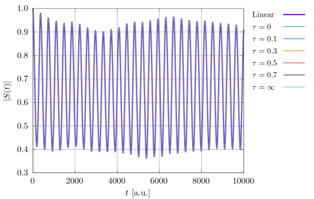
Figure 1: acf for the ivr of water described at the TDMVCC$[2]$ level. The reference calculation (purple) uses linearly parametrized modals, while the remaining calculations use single exponentially parametrized modals with a number of reset thresholds $\tau$ (see text). Note that the lines coincide so some are not visible.

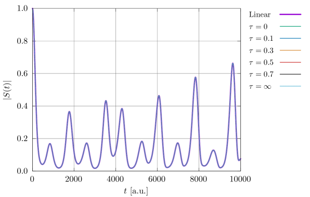
Figure 2: acf for the 5D trans-bithiophene model described at the TDMVCC$[2]$. The reference calculation (purple) uses linearly parametrized modals, while the remaining calculations use double exponentially parametrized modals with a number of reset thresholds $\tau$ (see text). Note that the lines coincide so some are not visible.

IV.3 Integrator step size

Having demonstrated the equivalence of the linear and exponential formalisms (and the correctness of the implementation) we turn to examine their performance and behaviour with respect to the integrator step size. Figure 3 shows the step size and the minimum eigenvalues $|\varphi^{m}_{\mathrm{min}}|$ of Eq. (79) for the water ivr calculation using single exponentially parametrized modals and $\tau=0$ (i.e. no resets). The step size exhibits a series of very sharp dips that coincide with small values of $|\varphi^{m}_{\mathrm{min}}|$. This is exactly the kind of near-singularity behaviour that was described in Sec. II.7. In this particular case, it seems that mode $1$ (i.e. the symmetric stretch, which was initially excited) is responsible for most near-singularities in the time interval shown. We note that the near-singularities are very short-lived and that the integrator is perfectly capable of stepping through them. This suggests that the formal existence of singularities in the modal eom is not catastrophic in a numerical setting. In Fig. 4, the water ivr calculation is repeated with $\tau=0.1$. The resets are clearly visible in the figure and have the effect of removing any (near-)singularities. As a consequence, the step size is stabilized close to its mean value.

Analogous results are shown for the 5D trans-bithiophene model in Figs. 5 and 6 (using double exponentially parametrized modals). A few near-singularities are also observed for this system but they are much less frequent compared to the water ivr case (this difference can be explained partially by the fact that the trans-bithiophene dynamics is simply slower). The near-singularities are again removed efficiently by the threshold-based resets.

Figures S1–S4 in the supplementary material show very similar behaviour for the ivr of water with double exponential modals and the 5D trans-bithiophene model with single exponential modals.

In order to assess performance in a more quantitative fashion we present average step sizes ($h_{\mathrm{mean}}$) for water and trans-bithiophene in Tables 1 and 2. The tables also include the mean stepsize relative to a reference calculation with linearly parametrized modals, i.e.

$$h_{\mathrm{rel}}=\frac{h_{\mathrm{mean}}}{h_{\mathrm{mean}}^{\mathrm{linear}}}.$$ (82)

For water (Table 1), the thresholds $\tau=0$ (no resets) and $\tau=\infty$ (reset after every step) perform slightly worse than the linear reference for single as well as double exponential calculations. Considering Fig. 3, it is perhaps not surprising that $\tau=0$ leads to smaller average steps due to the near-singularities. The remaining thresholds ($\tau=0.1,0.3,0.5,0.7$) all perform slightly better than the linear reference, although the difference is small (on the order of a few percent). The single and double exponential calculations perform essentially the same.

For trans-bithiophene (Table 2), all calculations with exponentially parametrized modals perform slightly better than the reference except for the single exponential calculation with $\tau=0$. The double exponentially parametrized modals result in slightly larger average steps compared to the single exponential case, but the difference is again small.

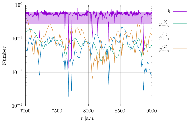
Figure 3: Integrator step size ($h$) and $|\varphi^{m}_{\mathrm{min}}|$ for the ivr of water described at the TDMVCC$[2]$ level using single exponentially parametrized modals ($\tau=0$, i.e. no resets). The shaded area covers the mean step size plus/minus its standard deviation (computed within the shown time interval). Only part of the full time interval is shown for greater visibility.

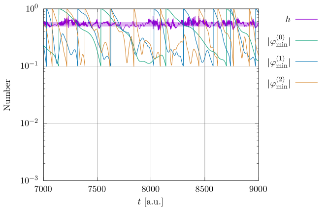
Figure 4: Integrator step size ($h$) and $|\varphi^{m}_{\mathrm{min}}|$ for the ivr of water described at the TDMVCC$[2]$ level using single exponentially parametrized modals ($\tau=0.1$). The shaded area covers the mean step size plus/minus its standard deviation (computed within the shown time interval). Only part of the full time interval is shown for greater visibility.

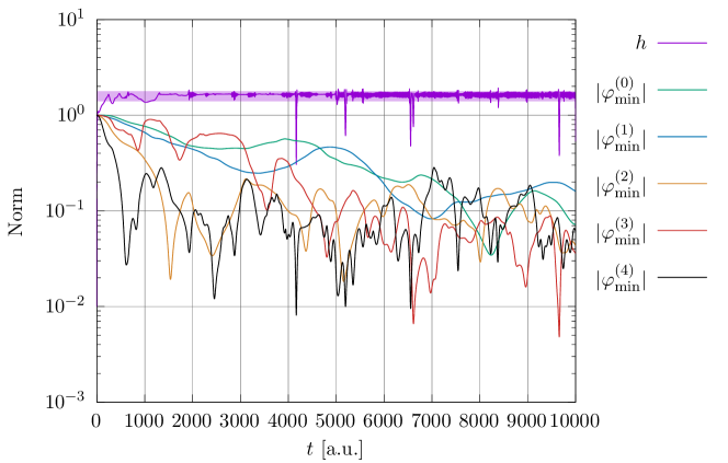
Figure 5: Integrator step size ($h$) and $|\varphi^{m}_{\mathrm{min}}|$ for the 5D trans-bithiophene model described at the TDMVCC$[2]$ level using double exponentially parametrized modals ($\tau=0$, i.e. no resets). The shaded area covers the mean step size plus/minus its standard deviation.

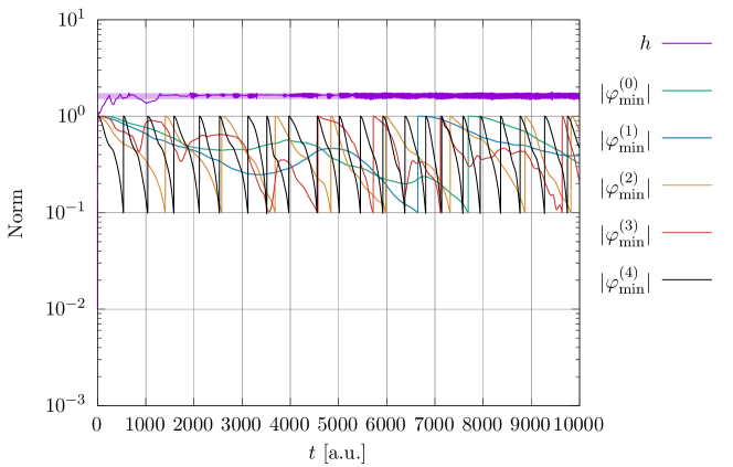
Figure 6: Integrator step size ($h$) and $|\varphi^{m}_{\mathrm{min}}|$ for the 5D trans-bithiophene model described at the TDMVCC$[2]$ level using double exponentially parametrized modals ($\tau=0.1$). The shaded area covers the mean step size plus/minus its standard deviation.

Table 1: Mean and relative step sizes for the ivr of water described at the TDMVCC$[2]$ level. $h_{\mathrm{mean}}$ is given in atomic units and $h_{\mathrm{rel}}$ is given relative to the linear case.

Type	$\tau$	$h_{\mathrm{mean}}$	$h_{\mathrm{rel}}$
Linear	—	$0.4088$	$1.0000$
Single	$0$	$0.3880$	$0.9491$
	$0.1$	$0.4182$	$1.0229$
	$0.3$	$0.4175$	$1.0211$
	$0.5$	$0.4151$	$1.0154$
	$0.7$	$0.4119$	$1.0075$
	$\infty$	$0.4080$	$0.9979$
Double	$0$	$0.3879$	$0.9488$
	$0.1$	$0.4178$	$1.0220$
	$0.3$	$0.4174$	$1.0210$
	$0.5$	$0.4151$	$1.0154$
	$0.7$	$0.4129$	$1.0099$
	$\infty$	$0.4079$	$0.9977$

Table 2: Mean and relative step sizes for the 5D trans-bithiophene model described at the TDMVCC$[2]$ level. $h_{\mathrm{mean}}$ is given in atomic units and $h_{\mathrm{rel}}$ is given relative to the linear case.

Type	$\tau$	$h_{\mathrm{mean}}$	$h_{\mathrm{rel}}$
Linear	—	$1.5704$	$1.0000$
Single	$0$	$1.5574$	$0.9917$
	$0.1$	$1.6075$	$1.0236$
	$0.3$	$1.6080$	$1.0240$
	$0.5$	$1.6088$	$1.0245$
	$0.7$	$1.6090$	$1.0246$
	$\infty$	$1.6100$	$1.0253$
Double	$0$	$1.5901$	$1.0126$
	$0.1$	$1.6184$	$1.0306$
	$0.3$	$1.6186$	$1.0308$
	$0.5$	$1.6194$	$1.0313$
	$0.7$	$1.6184$	$1.0306$
	$\infty$	$1.6202$	$1.0318$

V Summary and outlook

A general set of eom for time-dependent wave functions with exponentially parametrized biorthogonal basis sets has been derived in a fully bivariational framework. The non-trivial connection to the eom for linearly parametrized basis sets was elucidated, thus offering a unified perspective on the two approaches. In particular, it was shown that the computationally intensive parts are in fact identical for the two kinds of parametrizations. The exponential parametrization can thus be implemented on top of existing code with limited programming effort.

Careful analysis of the equations showed the existence of a well-defined set of singularities related to the eigenvalues of the matrices containing the basis set parameters. It was demonstrated how these singularities can be removed in a controlled manner by a simple update of the Hamiltonian integrals. The monitoring of singularities requires only quantities that are computed in any case.

The exponential eom were subsequently used as a starting point for deriving eom for a double exponential parametrization, thus providing a separation of the basis set time evolution into a unitary part and a part describing the deviation from unitarity. The transformations necessary to obtain the double exponential formulation again carry negligible additional cost.

Finally, we presented numerical results for calculations on water and a 5D trans-bithiophene model. The calculations showed that the single and double exponential parametrizations result in slightly larger step sizes compared to linearly parametrized reference calculations. Although the effect on step size is minor, our findings underline the fact that one should not necessarily consider the exponential basis set parametrization as more costly compared to the linear parametrization. We have argued that the additional operations needed for the exponential parametrization are computationally cheap, while an increase in the average itegrator step size leads directly to fewer costly evaluations of the eom.

Although the present work focuses on bivariational wave functions, we note that the mathematical machinery for converting between linearly and exponentially parametrized basis sets is also applicable to other types of wave functions. We thus anticipate that these results will be usefull in future treatments of both nuclear quantum dynamics and time-dependent electronic structure.

Supplementary material

The supplementary material contains additional figures related to the water and 5D trans-bithiophene calculations presented within the article.

Author declarations

Conflict of Interest

The authors have no conflicts to disclose.

Author Contributions

Mads Greisen Højlund: Conceptualization (equal); Data curation (lead); Formal analysis (equal); Investigation (lead); Software (lead); Visualization (lead); Writing – original draft (lead); Writing – review & editing (equal). Alberto Zoccante: Conceptualization (equal); Formal analysis (equal); Writing – review & editing (equal). Ove Christiansen: Conceptualization (equal); Formal analysis (equal); Funding acquisition (lead); Project administration (lead); Supervision (lead); Writing – review & editing (equal).

Data availability

The data that supports the findings of this study are available within the article and its supplementary material.

Appendix A Similarity transformed derivative: Specialization

Direct application of Eq. (51) shows that

$$D_{pq}=e^{-\hat{\kappa}}\partialderivative{e^{\hat{\kappa}}}{\kappa_{pq}}=\sum_{rs}d_{(pq)(rs)}E_{rs}$$ (A1)

where we have reintroduced explicit summation and left out the mode index $m$ to avoid notational clutter. This is identical to Eq. (II.3) but now includes a concrete recipe for computing the $\mathbf{D}$ matrix. In order to actually carry out the computation we need to consider the structure constants describing the generators $E_{pq}$. By writing

$$[E_{pq},E_{rs}] =\delta_{qr}E_{ps}-\delta_{ps}E_{rq}$$ (A2)

$$=\sum_{\bar{r}\bar{s}}(\delta_{qr}\delta_{\bar{r}p}\delta_{\bar{s}s}-\delta_{ps}\delta_{\bar{r}r}\delta_{\bar{s}q})E_{\bar{r}\bar{s}}$$ (A3)

we see that

$$f^{\bar{r}\bar{s}}_{(pq)(rs)}=(\delta_{qr}\delta_{\bar{r}p}\delta_{\bar{s}s}-\delta_{ps}\delta_{\bar{r}r}\delta_{\bar{s}q}).$$ (A4)

The $\mathbf{Q}$ matrix is now given by

$$Q_{(rs)(\bar{r}\bar{s})} =\sum_{pq}\kappa_{pq}f^{\bar{r}\bar{s}}_{(pq)(rs)}$$

$$=\sum_{pq}\kappa_{pq}\delta_{qr}\delta_{\bar{r}p}\delta_{\bar{s}s}-\sum_{pq}\kappa_{pq}\delta_{ps}\delta_{\bar{r}r}\delta_{\bar{s}q}$$

$$=\kappa_{\bar{r}r}\delta_{\bar{s}s}-\kappa_{s\bar{s}}\delta_{\bar{r}r}$$ (A5)

or, equivalently,

$$\mathbf{Q} =\mathbf{K}^{\mspace{-3.0mu}\mathsf{T}}\otimes\mathbf{1}-\mathbf{1}\otimes\mathbf{K}$$

$$=\mathbf{K}^{\mspace{-3.0mu}\mathsf{T}}\otimes\mathbf{1}+\mathbf{1}\otimes(-\mathbf{K})$$

$$=\mathbf{K}^{\mspace{-3.0mu}\mathsf{T}}\oplus(-\mathbf{K}).$$ (A6)

Here, $\otimes$ denotes the Kronecker product while $\oplus$ denotes the so-called Kronecker sum. The simple structure in Eq. (A) allows us to analyse and manipulate the $\mathbf{Q}$ matrix in a convenient way. Let $\mathbf{K}$ have eigenvalues $\mu_{1},\ldots,\mu_{N}$ where $N$ is the order of the matrix. Then $-\mathbf{K}$ has eigenvalues $-\mu_{1},\ldots,-\mu_{N}$ while $\mathbf{Q}$ has eigenvalues(Laub, 2005)

$$\lambda_{pq}=\mu_{p}-\mu_{q},\quad p,q=1,\ldots,N.$$ (A7)

We see that $\mathbf{Q}$ has at least $N$ eigenvalues equal to zero and so $\mathbf{Q}$ is always singular. Now assume that $\mathbf{K}$ is diagonalizable as

$$\mathbf{K} =\mathbf{R}\bm{\mu}\mathbf{L}^{\dagger},\quad\mathbf{L}^{\dagger}\mathbf{R}=\mathbf{R}\mathbf{L}^{\dagger}=\mathbf{1}$$ (A8)

where $\bm{\mu}$ is a diagonal matrix holding the eigenvalues $\mu_{p}$. In the notation of Eq. (A8), the rows of $\mathbf{L}^{\dagger}$ are the left eigenvectors of $\mathbf{K}$ while the columns of $\mathbf{V}$ are the right eigenvectors of $\mathbf{K}$. In addition, let

$$\bm{\Lambda}=\bm{\mu}\otimes\mathbf{1}-\mathbf{1}\otimes\bm{\mu}$$ (A9)

be the diagonal matrix holding the eigenvalues $\lambda_{pq}=\mu_{p}-\mu_{q}$ of $\mathbf{Q}$. It follows directly that

$$(\mathbf{L}^{*}\otimes\mathbf{R})\bm{\Lambda}(\mathbf{R}^{\mspace{-3.0mu}\mathsf{T}}\otimes\mathbf{L}^{\dagger}) =(\mathbf{L}^{*}\otimes\mathbf{R})(\bm{\mu}\otimes\mathbf{1}-\mathbf{1}\otimes\bm{\mu})(\mathbf{R}^{\mspace{-3.0mu}\mathsf{T}}\otimes\mathbf{L}^{\dagger})$$

$$=(\mathbf{L}^{*}\bm{\mu}\mathbf{R}^{\mspace{-3.0mu}\mathsf{T}})\otimes(\mathbf{R}\mathbf{L}^{\dagger})-(\mathbf{L}^{*}\mathbf{R}^{\mspace{-3.0mu}\mathsf{T}})\otimes(\mathbf{R}\bm{\mu}\mathbf{L}^{\dagger})$$

$$=\mathbf{K}^{\mspace{-3.0mu}\mathsf{T}}\otimes\mathbf{1}-\mathbf{1}\otimes\mathbf{K}$$

$$=\mathbf{Q}.$$ (A10)

We see that $\mathbf{Q}$ can be diagonalized in a simple way provided $\mathbf{K}$ is diagonalizable. The matrices

$$\bm{\mathfrak{R}} =\mathbf{L}^{*}\otimes\mathbf{R}$$ (A11a)

$$\bm{\mathfrak{L}}^{\dagger} =\mathbf{R}^{\mspace{-3.0mu}\mathsf{T}}\otimes\mathbf{L}^{\dagger}$$ (A11b)

contain the right and left eigenvectors of $\mathbf{Q}$, respectively, and satisfy $\bm{\mathfrak{L}}^{\dagger}\bm{\mathfrak{R}}=\bm{\mathfrak{R}}\bm{\mathfrak{L}}^{\dagger}=\mathbf{1}$ due to Eq. (A8). Following Eq. (52), we are now ready to compute

$$\mathbf{D} =\bm{\mathfrak{R}}\varphi(\bm{\Lambda})\bm{\mathfrak{L}}^{\dagger} =\bm{\mathfrak{R}}\mathbf{\Phi}\bm{\mathfrak{L}}^{\dagger},$$ (A12a)

$$\mathbf{D}^{\mspace{-3.0mu}\mathsf{T}} =\bm{\mathfrak{L}}^{*}\varphi(\bm{\Lambda})\bm{\mathfrak{R}}^{\mspace{-3.0mu}\mathsf{T}} =\bm{\mathfrak{L}}^{*}\mathbf{\Phi}\bm{\mathfrak{R}}^{\mspace{-3.0mu}\mathsf{T}}$$ (A12b)

where the diagonal matrix $\mathbf{\Phi}$ has diagonal elements

$$\varphi_{pq}=\varphi(\lambda_{pq})=\varphi(\mu_{p}-\mu_{q}).$$ (A13)

If $\mathbf{D}$ and thus $\mathbf{D}^{\mspace{-3.0mu}\mathsf{T}}$ is invertible, we write

$$\mathbf{D}^{-\mspace{-3.0mu}\mathsf{T}}=\bm{\mathfrak{L}}^{*}\mathbf{\Phi}^{-1}\bm{\mathfrak{R}}^{\mspace{-3.0mu}\mathsf{T}}$$ (A14)

and proceed to compute the matrix-vector product

$$\dot{\bm{\kappa}} =-i\mathbf{D}^{-\mspace{-3.0mu}\mathsf{T}}\mathbf{g}$$

$$=-i\bm{\mathfrak{L}}^{*}\mathbf{\Phi}^{-1}\bm{\mathfrak{R}}^{\mspace{-3.0mu}\mathsf{T}}\mathbf{g}$$

$$=-i(\mathbf{R}\otimes\mathbf{L}^{*})\mathbf{\Phi}^{-1}(\mathbf{L}^{\dagger}\otimes\mathbf{R}^{\mspace{-3.0mu}\mathsf{T}})\mathbf{g}.$$ (A15)

This exact type of product was encountered in the appendix of Ref. 36 and can be simplified by using that

$$(\mathbf{A}\otimes\mathbf{B})\mathrm{vec}(\mathbf{C})=\mathrm{vec}(\mathbf{A}\mathbf{C}\mathbf{B}^{\mspace{-3.0mu}\mathsf{T}})$$ (A16)

where $\mathrm{vec}(\cdot)$ denotes the row-major vectorization mapping. Rather than repeating the steps, we simply state the result:

$$\dot{\mathbf{K}}=-i\mathbf{R}\big{(}\mathbf{\Omega}\circ\big{(}\mathbf{L}^{\dagger}\mathbf{G}\mathbf{R}\big{)}\big{)}\mathbf{L}^{\dagger}.$$ (A17)

Here, $\dot{\mathbf{K}}$ and $\mathbf{G}$ are the matrices holding the elements of the vectors $\dot{\bm{\kappa}}$ and $\mathbf{g}$, respectively, while the symbol $\circ$ denotes the Hadamard (or element-wise) product. We have, in addition, introduced the $N\times N$ matrix $\mathbf{\Omega}$ that holds the $N^{2}$ diagonal elements of the $N^{2}\times N^{2}$ diagonal matrix $\mathbf{\Phi}^{-1}$, i.e.

$$\omega_{pq}=1/\varphi(\lambda_{pq})=1/\varphi(\mu_{p}-\mu_{q}).$$ (A18)

This result holds, as mentioned, when $\mathbf{D}^{\mspace{-3.0mu}\mathsf{T}}$ is invertible. According to the discussion in Sec. II.4, this is the case exactly when

$$\mu_{p}-\mu_{q}\neq 2\pi ik$$ (A19)

where $k$ is a non-zero integer.

References

- Zgid and Nooijen (2008) D. Zgid and M. Nooijen, J. Chem. Phys. 128, 144116 (2008).
- Ghosh et al. (2008) D. Ghosh, J. Hachmann, T. Yanai, and G. K.-L. Chan, J. Chem. Phys. 128, 144117 (2008).
- Ma et al. (2017) Y. Ma, S. Knecht, S. Keller, and M. Reiher, J. Chem. Theory Comput. 13, 2533 (2017).
- Sherrill et al. (1998) C. D. Sherrill, A. I. Krylov, E. F. C. Byrd, and M. Head-Gordon, J. Chem. Phys. 109, 4171 (1998).
- Pedersen, Koch, and Hättig (1999) T. B. Pedersen, H. Koch, and C. Hättig, J. Chem. Phys. 110, 8318 (1999).
- Pedersen, Fernández, and Koch (2001) T. B. Pedersen, B. Fernández, and H. Koch, J. Chem. Phys. 114, 6983 (2001).
- Arponen (1983) J. Arponen, Ann. Phys. 151, 311 (1983).
- Myhre (2018) R. H. Myhre, J. Chem. Phys. 148, 094110 (2018).
- Köhn and Olsen (2005) A. Köhn and J. Olsen, J. Chem. Phys. 122, 084116 (2005).
- Meyer, Manthe, and Cederbaum (1990) H.-D. Meyer, U. Manthe, and L. Cederbaum, Chem. Phys. Lett. 165, 73 (1990).
- Beck et al. (2000) M. H. Beck, A. Jäckle, G. A. Worth, and H.-D. Meyer, Phys. Rep. 324, 1 (2000).
- Zanghellini et al. (2003) J. Zanghellini, M. Kitzler-Zeiler, C. Fabian, T. Brabec, and A. Scrinzi, Laser Phys. 13, 1064 (2003).
- Caillat et al. (2005) J. Caillat, J. Zanghellini, M. Kitzler, O. Koch, W. Kreuzer, and A. Scrinzi, Phys. Rev. A 71, 012712 (2005).
- Kato and Kono (2004) T. Kato and H. Kono, Chem. Phys. Lett. 392, 533 (2004).
- Sato and Ishikawa (2013) T. Sato and K. L. Ishikawa, Phys. Rev. A 88, 023402 (2013).
- Miyagi and Madsen (2013) H. Miyagi and L. B. Madsen, Phys. Rev. A 87, 062511 (2013).
- Haxton and McCurdy (2015) D. J. Haxton and C. W. McCurdy, Phys. Rev. A 91, 012509 (2015).
- Sato and Ishikawa (2015) T. Sato and K. L. Ishikawa, Phys. Rev. A 91, 023417 (2015).
- Worth (2000) G. A. Worth, J. Chem. Phys. 112, 8322 (2000).
- Wodraszka and Carrington (2016) R. Wodraszka and T. Carrington, J. Chem. Phys. 145, 044110 (2016).
- Larsson and Tannor (2017) H. R. Larsson and D. J. Tannor, J. Chem. Phys. 147, 044103 (2017).
- Madsen et al. (2020a) N. K. Madsen, M. B. Hansen, G. A. Worth, and O. Christiansen, J. Chem. Phys. 152, 084101 (2020a).
- Madsen et al. (2020b) N. K. Madsen, M. B. Hansen, G. A. Worth, and O. Christiansen, J. Chem. Theory Comput. 16, 4087 (2020b).
- Alon, Streltsov, and Cederbaum (2007) O. E. Alon, A. I. Streltsov, and L. S. Cederbaum, Phys. Rev. A 76, 062501 (2007).
- Alon, Streltsov, and Cederbaum (2008) O. E. Alon, A. I. Streltsov, and L. S. Cederbaum, Phys. Rev. A 77, 033613 (2008).
- Nest (2009) M. Nest, Chemical Physics Letters 472, 171 (2009).
- Manthe and Weike (2017) U. Manthe and T. Weike, J. Chem. Phys. 146, 064117 (2017).
- Kvaal (2012) S. Kvaal, J. Chem. Phys. 136, 194109 (2012).
- Sato et al. (2018) T. Sato, H. Pathak, Y. Orimo, and K. L. Ishikawa, J. Chem. Phys. 148, 051101 (2018).
- Pedersen and Kvaal (2019) T. B. Pedersen and S. Kvaal, J. Chem. Phys. 150, 144106 (2019).
- Kristiansen et al. (2020) H. E. Kristiansen, Ø. S. Schøyen, S. Kvaal, and T. B. Pedersen, J. Chem. Phys. 152, 071102 (2020).
- Pathak, Sato, and Ishikawa (2020) H. Pathak, T. Sato, and K. L. Ishikawa, J. Chem. Phys. 153, 034110 (2020).
- Pathak, Sato, and Ishikawa (2021) H. Pathak, T. Sato, and K. L. Ishikawa, J. Chem. Phys. 154, 234104 (2021).
- Kristiansen et al. (2022) H. E. Kristiansen, B. S. Ofstad, E. Hauge, E. Aurbakken, Ø. S. Schøyen, S. Kvaal, and T. B. Pedersen, J. Chem. Theory Comput. 18, 3687 (2022).
- Madsen et al. (2020c) N. K. Madsen, M. B. Hansen, O. Christiansen, and A. Zoccante, J. Chem. Phys. 153, 174108 (2020c).
- Højlund et al. (2022) M. G. Højlund, A. B. Jensen, A. Zoccante, and O. Christiansen, J. Chem. Phys. 157, 234104 (2022).
- Helgaker, Jørgensen, and Olsen (2000) T. Helgaker, P. Jørgensen, and J. Olsen, Molecular Electronic-Structure Theory (Wiley, Chichester ; New York, 2000).
- Pedersen and Koch (1998) T. B. Pedersen and H. Koch, J. Chem. Phys. 108, 12 (1998).
- Madsen et al. (2018) N. K. Madsen, M. B. Hansen, A. Zoccante, K. Monrad, M. B. Hansen, and O. Christiansen, J. Chem. Phys. 149, 134110 (2018).
- Kramer and Saraceno (1981) P. Kramer and M. Saraceno, Geometry of the Time-Dependent Variational Principle in Quantum Mechanics, Lecture Notes in Physics, Vol. 140 (Springer Berlin Heidelberg, Berlin, Heidelberg, 1981).
- Ohta (2004) K. Ohta, Phys. Rev. A 70, 022503 (2004).
- Christiansen (2004) O. Christiansen, J. Chem. Phys. 120, 2140 (2004).
- Hall (2015) B. C. Hall, Lie Groups, Lie Algebras, and Representations, Graduate Texts in Mathematics, Vol. 222 (Springer International Publishing, Cham, 2015).
- Olsen and Jørgensen (1985) J. Olsen and P. Jørgensen, J. Chem. Phys. 82, 3235 (1985).
- Hansen, Madsen, and Christiansen (2020) M. B. Hansen, N. K. Madsen, and O. Christiansen, J. Chem. Phys. 153, 044133 (2020).
- Olsen (2015) J. Olsen, J. Chem. Phys. 143, 114102 (2015).
- Laub (2005) A. J. Laub, Matrix Analysis for Scientists and Engineers (Society for Industrial and Applied Mathematics, Philadelphia, 2005).
- Hairer, Nørsett, and Wanner (2009) E. Hairer, S. P. Nørsett, and G. Wanner, Solving Ordinary Differential Equations I: Nonstiff Problems, 2nd ed., Springer Series in Computational Mathematics No. 8 (Springer, Heidelberg ; London, 2009).
- Hairer, Lubich, and Wanner (2006) E. Hairer, C. Lubich, and G. Wanner, Geometric Numerical Integration: Structure-Preserving Algorithms for Ordinary Differential Equations, 2nd ed., Springer Series in Computational Mathematics No. 31 (Springer, Berlin ; New York, 2006).
- Artiukhin et al. (2022) D. G. Artiukhin, O. Christiansen, I. H. Godtliebsen, E. M. Gras, W. Győrffy, M. B. Hansen, M. B. Hansen, E. L. Klinting, J. Kongsted, C. König, D. Madsen, N. K. Madsen, K. Monrad, G. Schmitz, P. Seidler, K. Sneskov, M. Sparta, B. Thomsen, D. Toffoli, A. Zoccante, M. G. Højlund, N. M. Høyer, and A. B. Jensen, “MidasCpp,” (2022).
- Madsen et al. (2019) D. Madsen, O. Christiansen, P. Norman, and C. König, Phys. Chem. Chem. Phys. 21, 17410 (2019).