Classical-to-quantum non-signalling boxes

Abstract

Here we introduce the concept of classical input - quantum output (C-Q) non-signalling boxes, a generalisation of the classical input - classical output (C-C) non-signalling boxes. We argue that studying such objects leads to a better understanding of the relation between quantum nonlocality and non-locality beyond quantum mechanics. The main issue discussed in the paper is whether there exist “genuine” C-Q boxes or all C-Q boxes can be built from objects already known, namely C-C boxes acting on pre-shared entangled quantum particles. We show that large classes of C-Q boxes are non-genuine. In particular, we show that all bi-partite C-Q boxes with outputs that are pure states are non-genuine. We also present various strategies for addressing the general problem, whose answer is still open. Surprising results concerning tri-partite C-Q boxes that follow from this approach are also presented. Finally, we show that simulating even very simple C-Q boxes requires large amounts of C-C nonlocal correlations.

I Introduction

During the recent years, the existence of long-distance nonlocal correlations, first discovered by J. Bell bell and experimentally confirmed by S.J. Freedman and J.F. Clauser clauser exp and A. Aspect, P.Grangier and G.Roger aspect became to be understood as one of the main aspects of nature. Very intensive research has taken place in the subject, from understanding the various aspects of entanglement and Bell inequalities to making use of nonlocality in virtually in all of quantum information tasks and even to leading to new insights in quantum gravity.

To further compound the surprise of the very existence of nonlocality, it has been later realised that nonlocal correlations even stronger than those allowed by quantum mechanics could in principle exist without entering in conflict with relativity PR . This has raised fundamental questions about Nature. Perhaps such correlations exist in Nature, only we have not discovered them yet. If discovered, it would mean that quantum mechanics is not a valid description of Nature and needs to be replaced by another theory. On the other hand, if such correlations do not exist, why don’t they exist? As they are not in contradiction with relativity, what other fundamental principles of nature rule them out?

One fruitful approach to the above question has been to consider “non-signalling boxes”, hypothetical boxes that accept classical inputs and yield classical outputs that are non-locally correlated with each other PR barrett . Then try to find tasks to which they would be useful when the correlations are stronger than those allowed by quantum mechanics. It has been discovered that some tasks, mostly of information processing nature, with no relation whatsoever with quantum mechanics, have qualitatively different behaviour when allowed access to such boxes van dam , brassard . Tantalisingly, some tasks underwent a qualitative change precisely at the border of quantum to beyond quantum correlation strengths quantum limits from swapping ; information causality ; non-local computation . This already shows that quantum mechanics is a very special theory from a fundamental point of view, unrelated to “physical” properties such as structure of atoms, etc. Yet not the entire boundary of the set of quantum correlations has been singled out in this way. It is therefore quite important, in order to make progress along this line, to find new tasks and/or different ways to characterise nonlocality.

Here we introduce a (potentially) new type of non-signalling, non-local “boxes”. The boxes have classical inputs and they output quantum particles in given correlated states, depending on the inputs Fig 1.

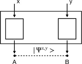
Figure 1: A CQ box has two parts, taking inputs x and y. It outputs a quantum state $\left|\Psi^{x,y}\right\rangle_{AB}$, joint across A and B.

In order for the box to be non-signalling, the reduced density matrix of each party must be independent on the input of the other party:

$$\begin{split}\rho^{x,y}_{A}=\rho^{x}_{A}\\ \rho^{x,y}_{B}=\rho^{y}_{B}\end{split}$$ (1)

where $\rho^{x,y}_{A}={\rm Tr}_{B}\rho^{x,y}_{A,B}$ and $\rho^{x,y}_{B}={\rm Tr}_{A}\rho^{x,y}_{A,B}$. In the case of multiple parties we generalise these conditions to say that the density matrices of all subgroups of parties could not depend on the inputs to the other parties.

Coming now to the crucial question of this paper, we said above that the C-Q boxes are “potentially new” because at the moment we do not know if there exist (theoretically) such genuine classically-quantum (C-Q) non-signalling boxes, or all of them could be decomposed in already known objects. Addressing this question is the core of the present paper.

Regardless of the answer, there are several reasons for considering such boxes. Quantum states have properties that are not captured by the formalism of the standard classical input-classical output (C-C) non-signalling boxes. While C-C non-signalling boxes can present correlations stronger than those allowed by classical mechanics, their dynamics is far more limited than that of the quantum states barrett 2010 . In particular, while nonlocality swapping (algebraically described by entanglement swapping) is possible in quantum mechanics, it is not possible for C-C boxes short . Obviously then, if genuine C-Q non-signalling boxes exist, they will extend the range of non-local phenomena that we thought to be possible in a non-deterministic world, while being consistent with relativity. On the other hand, if genuine C-Q boxes do not exist another set of interesting questions follow. First, what are the resources needed to implement them via C-C boxes and pre-shared entanglement? As we will show, in some cases it seems that these resources need to be extremely large. Second, and more important, why do genuine C-Q boxes not exist? Why is it that the most nonlocal non-signalling device with quantum output is an ordinary pairing of a C-C non-signalling device and pre-shared entanglement.

As for the answer, the question of the existence of genuine C-Q boxes is still open.

The main result of our paper is that all bi-partite C-Q boxes whose outputs are pure states are not genuine, ruling out one of the major class of situations. To put the result in context, most of the major results concerning non-locality in the traditional classical input-classical output (C-C) scenario, starting with the very discovery by J. Bell of the existence of nonlocality, have been obtained in the bi-partite, pure state situations. One would have expected that if the extension of non-locality to classical input-quantum output situations (C-Q) brings something new, this should already be evident from the extension of this simpler class which, as we show, is not the case.

At the same time, it is also the case that in the C-C scenario mixed states and multi-partite situations manifest qualitatively new phenomena with respect to the bi-partite, pure state situation. It is thus conceivable that the C-Q scenario in these more general situations does contain genuine C-Q effects that cannot be simulated by using C-C correlations. Here we only have partial results. For bi-partite C-Q boxes with mixed state outputs we shall present various paradigmatic examples of boxes which turn out to be non-genuine. We also present some surprising results for tri-partite situations.

Along the way of proving the above results, our paper sets up the general strategy for investigating C-Q non-locality and exposes basic structures of C-Q boxes. As a by-product we also draw the attention to a novel class of C-C boxes, extensions of the PR boxes which have been a main tool in the study of non-locality.

II Non-genuine C-Q boxes

Obviously, some C-Q boxes could be obtained by a combination of pre-shared entangled quantum states and a classical-classical non-signalling box, which are encapsulated in a bigger box so that from the outside one doesn’t see this combination, as illustrated in fig 2.

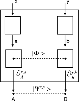
Figure 2: Example of a non-genuine C-Q box, constructed from a C-C box (which takes inputs x,y and outputs a,b), a pre-shared entangled state $\left|\Phi\right\rangle$, and some local unitaries ${\hat{U}}^{x,a}_{A}$ and ${\hat{U}}^{y,b}_{B}$ that are applied to $\left|\Phi\right\rangle$ to generate the desired state $\left|\Psi^{x,y}\right\rangle$. In general ancillas may be also included inside the box.

Specifically, the inputs $x$ and $y$ are plugged in the C-C box, which gives outputs $a$ and $b$. Then Alice applies some unitary transformation ${\hat{U}}^{x,a}_{A}$ to her quantum particle depending on her input $x$ and the C-C box output $a$ and finally outputs her quantum particle out of the bigger box. Bob follows a similar procedure. Internal ancillas could also be added. From the outside this combination looks as a C-Q box. We call these “non-genuine” classical-quantum boxes.

III Examples of boxes with pure states outputs

We present a few examples of boxes, of increasing complexity, which turn out to be non-genuine. This will show the main ideas of how to create the desired boxes and show that they are non-genuine.

III.1 QM correlations are not enough

As a first example consider inputs $x,y=0,1$ and the C-Q box defined by

$$\begin{split}x\cdot y=0\rightarrow\frac{1}{\sqrt{2}}(\left|0\right\rangle\left|0\right\rangle+\left|1\right\rangle\left|1\right\rangle)\\ x\cdot y=1\rightarrow\frac{1}{\sqrt{2}}(\left|0\right\rangle\left|1\right\rangle+\left|1\right\rangle\left|0\right\rangle)\end{split}$$ (2)

where $\left|0\right\rangle\left|1\right\rangle$ is short for $\left|0\right\rangle_{A}\left|1\right\rangle_{B}$.

Note that this box cannot be created with only shared entanglement and no other non-local resources such as C-C boxes, as one can make the PR box

$$(a-b)mod~{}2=x\cdot y$$ (3)

from this by measuring in the $0/1$ basis, and the PR box (which one example of a C-C box) is known to give stronger than quantum correlations.

This box however is a non-genuine C-Q one since it can be simulated by the PR box above plus the pre-shared maximally entangled state $\left|\Phi\right\rangle=\frac{1}{\sqrt{2}}(\left|0\right\rangle\left|0\right\rangle+\left|1\right\rangle\left|1\right\rangle)$. Alice simply needs to apply the bit flip operator $U_{A}$ (which flips $\left|0\right\rangle$ to $\left|1\right\rangle$ and vice versa) to $A$ whenever the PR box gives $a=1$. Similarly Bob applies the same bit flip operator $U_{B}$ to $B$ whenever $b=1$. When $x\cdot y=0$ the PR box gives $a=b$, so Alice and Bob will either both flip or neither flip their qubits, and both operations leave $\left|\Phi\right\rangle$ unchanged. When $x\cdot y=1$ only one of Alice or Bob will flip their bits and we will have $\frac{1}{\sqrt{2}}(\left|0\right\rangle\left|1\right\rangle+\left|1\right\rangle\left|0\right\rangle)$ as desired.

III.2 Sign flip

Next consider inputs $x,y=0,1$ and the box which outputs states $\left|\Psi^{x,y}\right\rangle$ according to

$$\left|\Psi^{x,y}\right\rangle=\alpha\left|0\right\rangle\left|0\right\rangle+\beta e^{i\pi x\cdot y}\left|1\right\rangle\left|1\right\rangle.$$ (4)

This can be simulated by a PR box $(a-b)mod2=x\cdot y$. Alice and Bob apply ${\hat{U}}^{a}_{A}$ and ${\hat{V}}^{b}_{B}$ respectively to the initial state $\left|\Psi\right\rangle=\alpha\left|0\right\rangle\left|0\right\rangle+\beta\left|1\right\rangle\left|1\right\rangle)$ where

$${\hat{U}}^{a}_{A}\left|0\right\rangle_{A} =\left|0\right\rangle_{A} {\hat{V}}^{b}_{B}\left|0\right\rangle_{B} =\left|0\right\rangle_{B}$$ (5)

$${\hat{U}}^{a}_{A}\left|1\right\rangle_{A} =e^{i\pi a}\left|1\right\rangle_{A} {\hat{V}}^{b}_{B}\left|1\right\rangle_{B} =e^{-i\pi b}\left|1\right\rangle_{B}$$

which leads to

$$\begin{split}\left|\Psi\right\rangle\rightarrow{\hat{U}}^{a}_{A}{\hat{U}}^{b}_{B}\left|\Psi\right\rangle&=\alpha\left|0\right\rangle\left|0\right\rangle+\beta e^{i\pi(a-b)}\left|1\right\rangle\left|1\right\rangle\\ &=\alpha\left|0\right\rangle\left|0\right\rangle+\beta e^{i\pi((a-b)mod2)}\left|1\right\rangle\left|1\right\rangle\\ &=\alpha\left|0\right\rangle\left|0\right\rangle+\beta e^{i\pi x\cdot y}\left|1\right\rangle\left|1\right\rangle\end{split}$$ (6)

which is the desired state.

III.3 Phase change

The sign change in the previous example can be generalized to an arbitrary rational phase parameterized by $\theta$:

$$\left|\Psi^{x,y}\right\rangle=\alpha\left|0\right\rangle\left|0\right\rangle+\beta e^{i2\pi\theta x\cdot y}\left|1\right\rangle\left|1\right\rangle.$$ (7)

In the previous case $\theta=1/2$. Suppose now $\theta=1/4$. It is simple to see that using a standard PR box one cannot implement this C-Q box. Does this mean that this box is genuine C-Q? No. To decide that a C-Q box is genuine we need to show that there is no way to construct it by using a standard classical-classical box and using its outputs to implement appropriate local unitary operations on a pre-shared entangled quantum state. In our case it turns out that this is possible.

The desired C-Q box can be constructed by the use of a C-C box which takes inputs $x,y=0,1$ and gives outputs $a,b=0,1,2,3$ according to $(a-b)mod~{}4=x\cdot y$, with all pairs of outcomes that respect this constraints being given with equal probability (1/4 in this case). Alice then performs the rotation ${\hat{U}}^{a}_{A}\left|1\right\rangle_{A}=e^{i2\pi a/4}\left|1\right\rangle_{A}$ and Bob ${\hat{V}}^{b}_{B}\left|1\right\rangle_{B}=e^{i2\pi(-b)/4}\left|1\right\rangle_{B}$. This gives

$$\begin{split}\left|\Psi\right\rangle&\rightarrow\alpha\left|0\right\rangle\left|0\right\rangle+\beta e^{i2\pi(a-b)/4}\left|1\right\rangle\left|1\right\rangle\\ &=\alpha\left|0\right\rangle\left|0\right\rangle+\beta e^{i2\pi x\cdot y/4}\left|1\right\rangle\left|1\right\rangle\end{split}$$ (8)

as desired.

For other rational values of $\theta$, i.e. $\theta=\frac{m}{n}$ where $m$ and $n$ are integers, we can use a similar box with m dimensional outputs giving $(a-b)mod~{}n=x\cdot y$ and rotation ${\hat{U}}^{a}_{A}\left|1\right\rangle_{A}=e^{i2\pi am/n}\left|1\right\rangle_{A}$.

III.4 Phase change boxes and use of resources

As we have seen before, any phase change box with $\theta$ equal to a rational number, $\theta=\frac{m}{n}$, can be realised by a C-C box and unitary transformations, provided that we use a C-C box with $n$ outcomes. When $n$ is large, this C-C box is a large amount of non-local resources. One might ask whether there is a more efficient way to implement this C-Q box. However we shall show here that this is the most efficient possible implementation, both in terms of C-C box and entanglement.

Proving that to implement a phase change box with $\theta=\frac{1}{n}$ we require a C-C box with $a$ and $b$ each having $n$ outcomes, defined by $(a-b)mod~{}n=x\cdot y$, proceeds as follows.

First, assume that the procedure is implemented by starting with $\left|\Psi\right\rangle=\alpha\left(\left|0\right\rangle\left|0\right\rangle+\beta\left|1\right\rangle\left|1\right\rangle\right)$, and applying unitary operations ${\hat{U}}^{a}_{A}$ and ${\hat{V}}^{b}_{B}$ when the C-C box outputs $a$ and $b$. For simplicity we consider the case when $\alpha\neq\beta$, so the only operations that are allowed are only phase shifts. Furthermore, we can take the ${\hat{U}}^{a}_{A}$ to be different for different $a$, since otherwise we can use a simplified C-C box by merging them together, and similarly for Bob.

For the case $(x,y)=(0,0)$, when $a=0$, which occurs with some probability $p_{0}$, Alice applies ${\hat{U}}^{0}_{A}$. To generate $\left|\Psi^{+}\right\rangle$ Bob must apply $({\hat{U}}^{0}_{B})^{*}$, i.e. the complex conjugate. We can label his C-C box outcome $b=0$ in this case.

The next step is to realise that for the inputs $(x,y)=(0,0)$ the pair of outputs $(a,b)=(0,1)$ is redundant as Bob will need to apply the same unitary $({\hat{U}}^{0}_{B})^{*}$ as for $(a,b)=(0,0)$. Hence, for the inputs $(x,y)=0,0$ we will only consider $a=0$ to be paired with $b=0$. Similarly for $a=i$ when Alice applies ${\hat{U}}^{i}_{A}$, Bob must apply $({\hat{U}}^{i}_{B})^{*}$ and we can label his outcome $b=i$. So we can describe the C-C box in this $(x,y)=(0,0)$ case as outputting $a=b=i$ with probability $p_{i}$.

Due to no-signalling of the C-C box from Bob to Alice, comparing $(x,y)=(0,1)$ to $(0,0)$ we see that in the case $(0,1)$ Alice must receive outcome $a=i$ with the same probability $p_{i}$ as for the $(0,0)$ inputs, upon which she will apply ${\hat{U}}^{i}_{A}$. To keep $\left|\Psi^{+}\right\rangle$ unchanged the C-C box must output $b=a$, so that Bob applies $({\hat{U}}^{i}_{B})^{*}$. Similarly due to no-signalling from Alice to Bob, comparing $(x,y)=(1,0)$ to $(0,0)$ we see that in the case $(1,0)$ the C-C box must output $b=i$ with probability $p_{i}$, and to generate $\left|\Psi^{+}\right\rangle$ give $b=a$.

The important difference comes when considering the inputs $(x,y)=(1,1)$. Comparing $(1,0)$ to $(1,1)$ it is still the case that for $(x,y)=(1,1)$ Alice must receive outcome $a=i$ with probability $p_{i}$ and apply ${\hat{U}}^{i}_{A}$. And comparing $(0,1)$ to $(1,1)$ we see that for $(1,1)$ Bob must receive outcome $i$ with probability $p_{i}$ and apply $({\hat{U}}^{i}_{B})^{*}$.

However to generate the state $\left|\Psi^{1,1}\right\rangle=(\sigma^{2/n}_{z})_{A}\left|\Phi^{+}\right\rangle$ where $\sigma_{z}$ is the Pauli matrix which does

$$\begin{split}\left|0\right\rangle&\rightarrow\left|0\right\rangle\\ \left|1\right\rangle&\rightarrow e^{i\pi}\left|1\right\rangle,\end{split}$$ (9)

we need the C-C box to pair up $a$ and $b$ so that

$$\begin{split}({\hat{U}}^{b}_{B})^{*}{\hat{U}}^{a}_{A}\left|\Phi^{+}\right\rangle&={\hat{U}}^{a}_{A}({\hat{U}}^{b}_{A})^{\dagger}\left|\Phi^{+}\right\rangle\\ &=(\sigma^{2/n}_{z})_{A}\left|\Phi^{+}\right\rangle,\\ \implies{\hat{U}}^{a}_{A}&=(\sigma^{2/n}_{z})_{A}{\hat{U}}^{b}_{A}.\end{split}$$ (10)

Thus for any $i$, if ${\hat{U}}^{i}_{A}$ is one of the unitaries used in implementing the C-Q box, then $(\sigma^{2/n}_{z})_{A}{\hat{U}}^{i}_{A}$ is another one. The smallest set of ${\hat{U}}^{i}_{A}$ which has this property is the one where $i=0..n-1$ and

$${\hat{U}}^{i}_{A}=(\sigma^{2i/n}_{z})_{A}.$$ (11)

Given this set, we can create the desired state by pairing together $a$ and $b$ as

$$(a-b)mod~{}n=x\cdot y$$ (12)

which is a generalisation of the standard PR box that can be written also as $(a-b)mod~{}2=x\cdot y$.

This proves that if we implement the C-Q box in Eq (7) with $\theta=\frac{1}{n}$, using an initial $\left|\Phi^{+}\right\rangle$, local unitaries and a C-C box, then the C-C box needs to have dimension $n$ and be of the form $(a-b)mod~{}n=x\cdot y$. One could imagine starting with a different initial shared entangled state, but that will not help us to make a simpler box, as e.g. the unitaries we apply for $a=b=0$ for $x=y$ must create $\left|\Phi^{+}\right\rangle$ regardless, and the rest of the argument then proceeds as before. Thus any implementation of this C-Q box requires a C-C box with $n$ outputs.

III.5 Approximate C-C + entanglement implementation of C-Q boxes

In the previous subsections we have shown that various C-Q boxes are not genuine, since we were able to implement them via a C-C box and pre-shared entanglement. Here we introduce a new idea, the approximate C-C + entanglement implementation of a C-Q box. This is an important idea because it is likely that there are many C-Q boxes that cannot be implemented exactly by C-C + entanglement but can be implemented arbitrarily closely.

An example is that of phase change with irrational $\theta$. It is clear that we cannot implement the C-Q box via a C-C box with a finite number of different outputs. However, we can approximate any irrational $\theta$ arbitrarily closely by a rational number, and use the procedure described in the previous section to exactly implement this rational phase box.

An alternative method which implements the phase change for irrational $\theta$ exactly is to use a C-C box with $a$ and $b$ real numbers in $[0,1)$ satisfying $(a-b)mod~{}1=(x\cdot y)\theta$. This is a similar to going to the limit of of using a rational approximation and letting $n\rightarrow\infty$.

III.6 C-Q Box with maximally entangled outputs for each input.

Consider a C-Q box with maximally entangled outputs for each input.

Any arbitrary maximally entangled state can be written by acting on, say, Alice’s side with a unitary on a standard maximally entangled state. Using this representation we can define an arbitrary C-Q box with maximally entangled outputs as:

$$\begin{split}&\left|\Psi^{0,0}\right\rangle={\hat{\alpha}}_{A}\left|\Psi^{-}\right\rangle\\ &\left|\Psi^{0,1}\right\rangle={\hat{\beta}}_{A}\left|\Psi^{-}\right\rangle\\ &\left|\Psi^{1,0}\right\rangle={\hat{\gamma}}_{A}\left|\Psi^{-}\right\rangle\\ &\left|\Psi^{1,1}\right\rangle={\hat{\delta}}_{A}\left|\Psi^{-}\right\rangle,\end{split}$$ (13)

where $\left|\Psi^{-}\right\rangle=\frac{1}{\sqrt{2}}(\left|0\right\rangle\left|1\right\rangle-\left|1\right\rangle\left|0\right\rangle)$.

To show that this box is non-genuine C-Q we will show how to implement it using two steps, of which only the first uses a C-C box. First we will show how to implement a simplified version of the above box where ${\hat{\alpha}}_{A}={\hat{\beta}}_{A}={\hat{\gamma}}_{A}=\mathbf{1}$ and ${\hat{\delta}}_{A}=\hat{U}_{A}$ for an arbitrary $\hat{U}$.

This can be done by noting that any unitary on a $2$ dimensional system can be viewed in the Block sphere as a rotation by $\theta$ around a given axis, and the phase change implemented above is exactly such a rotation around the 0/1 axis. As $\left|\Psi^{-}\right\rangle$ is rotationally symmetric we can always write it as $\frac{1}{\sqrt{2}}\left(\left|\vec{n}\right\rangle\left|\vec{-n}\right\rangle-\left|\vec{-n}\right\rangle\left|\vec{n}\right\rangle\right)$ where $\vec{n}$ is the axis of rotation, and then use the the phase change box from the previous section to apply the rotation around that axis.

To implement the more general box in eq. (13) we shall next apply some local unitary operations. Alice applies ${\hat{\alpha}}_{A}$ when $x=0$ and ${\hat{\gamma}}_{A}$ when $x=1$, and Bob does nothing when $y=0$ and ${\hat{\beta}}^{\dagger}_{B}{\hat{\alpha}}_{B}$ when $y=1$. This gives us

$$\begin{split}&\left|\Psi^{0,0}\right\rangle={\hat{\alpha}}_{A}\left|\Psi^{-}\right\rangle\\ &\left|\Psi^{0,1}\right\rangle={\hat{\alpha}}_{A}{\hat{\beta}}^{\dagger}_{B}{\hat{\alpha}}_{B}\left|\Psi^{-}\right\rangle\\ &\left|\Psi^{1,0}\right\rangle={\hat{\gamma}}_{A}\left|\Psi^{-}\right\rangle\\ &\left|\Psi^{1,1}\right\rangle={\hat{\gamma}}_{A}{\hat{\beta}}^{\dagger}_{B}{\hat{\alpha}}_{B}{\hat{U}}_{A}\left|\Psi^{-}\right\rangle.\end{split}$$ (14)

Now note that due to the rotational symmetry of $\left|\Psi^{-}\right\rangle$ if Alice and Bob act on their particles with the same unitary operator ${\hat{U}}$, the state remains unchanged. So, in particular

$$\begin{split}{\hat{U}}_{A}{\hat{U}}_{B}\left|\Psi^{-}\right\rangle&=\left|\Psi^{-}\right\rangle\\ {\hat{U}}_{B}\left|\Psi^{-}\right\rangle&={\hat{U}}_{A}^{\dagger}\left|\Psi^{-}\right\rangle.\end{split}$$ (15)

Thus

$$\begin{split}\left|\Psi^{0,1}\right\rangle&={\hat{\alpha}}_{A}({\hat{\beta}}^{\dagger}_{A}{\hat{\alpha}}_{A})^{\dagger}\left|\Psi^{-}\right\rangle\\ &={\hat{\alpha}}_{A}{\hat{\alpha}}^{\dagger}_{A}{\hat{\beta}}_{A}\left|\Psi^{-}\right\rangle\\ &={\hat{\beta}}_{A}\left|\Psi^{-}\right\rangle,\end{split}$$ (16)

and

$$\begin{split}\left|\Psi^{1,1}\right\rangle&={\hat{\gamma}}_{A}{\hat{U}}_{A}{\hat{\beta}}^{\dagger}_{B}{\hat{\alpha}}_{B}\left|\Psi^{-}\right\rangle\\ &={\hat{\gamma}}_{A}{\hat{U}}_{A}({\hat{\beta}}^{\dagger}_{A}{\hat{\alpha}}_{A})^{\dagger}\left|\Psi^{-}\right\rangle\\ &={\hat{\gamma}}_{A}{\hat{U}}_{A}{\hat{\alpha}}^{\dagger}_{A}{\hat{\beta}}_{A}\left|\Psi^{-}\right\rangle.\end{split}$$ (17)

We can thus achieve $\left|\Psi^{1,1}\right\rangle={\hat{\delta}}_{A}\left|\Psi^{-}\right\rangle$ by setting ${\hat{U}}_{A}={\hat{\gamma}}^{\dagger}_{A}{\hat{\delta}}_{A}{\hat{\beta}}^{\dagger}_{A}{\hat{\alpha}}_{A}$.

Thus we have shown how to implement our C-Q box with maximally entangled outputs in terms of C-C boxes and local unitary operations.

Finally, we note that the protocol involves creating a phase change box to implement $U$. The resources used are therefore the ones necessary to implement the phase change, which depend on what the phase is as described in section III.4. They could be very large, and we can only implement $U$ approximately using a finite dimensional C-C box if the phase is irrational.

III.7 Higher Dimensions

We will now consider C-Q boxes with more inputs, say $x=0,1$ and $y=0,1,2$. This gives the hope to find a genuine C-Q box. The idea is that there have been already many constraints due to non-signalling in implementing via C-C + entanglement a C-Q box on the subset of inputs $x,y=0,1$ and that the input $y=2$ when paired with $x=0,1$ will add supplementary constraints that can no longer be fulfilled.

Consider the box

$$\begin{split}\left|\Psi^{00}\right\rangle=\left|\Psi^{01}\right\rangle=\left|\Psi^{02}\right\rangle=\left|\Psi^{10}\right\rangle&=\frac{1}{\sqrt{2}}(\left|0\right\rangle\left|0\right\rangle+\left|1\right\rangle\left|1\right\rangle)\\ \left|\Psi^{11}\right\rangle&=\hat{\sigma}_{z}^{1/2}\left|\Psi^{00}\right\rangle\\ \left|\Psi^{12}\right\rangle&=\hat{\sigma}_{x}\left|\Psi^{00}\right\rangle,\end{split}$$ (18)

where $\hat{\sigma}_{z}$ is the usual Pauli operator

$$\begin{split}\hat{\sigma}_{z}\left|0\right\rangle&=\left|0\right\rangle\\ \hat{\sigma}_{z}\left|1\right\rangle&=-\left|1\right\rangle,\end{split}$$ (19)

and $\hat{\sigma}_{x}$ flips the bits

$$\begin{split}\hat{\sigma}_{x}\left|0\right\rangle&=\left|1\right\rangle\\ \hat{\sigma}_{x}\left|1\right\rangle&=\left|0\right\rangle.\end{split}$$ (20)

This is the same as phase changes we handled in section III.3 for $(x,y)\in\{(0,0),(0,1),(1,0),(1,1)\}$. Thus we could construct that part from a pre-shared $\left|\Psi^{00}\right\rangle$ using the C-C box $(a-b)mod~{}4=x.y$, Alice applying the unitary operator

$$\{\mathbb{1},\hat{\sigma}_{z}^{1/2},\hat{\sigma}_{z}^{2/2},\hat{\sigma}_{z}^{3/2}\}$$ (21)

to $A$ when $a=0,1,2,3$ respectively, and Bob applying the inverse operator

$$\{\mathbb{1},\hat{\sigma}_{z}^{-1/2},\hat{\sigma}_{z}^{-2/2},\hat{\sigma}_{z}^{-3/2}\}$$ (22)

to $B$ when he sees $b=0,1,2,3$ respectively.

However in order to create $\left|\Psi^{12}\right\rangle$ when $(x,y)=(1,2)$ we need something which allows us to flip the bit, e.g. $\hat{\sigma}_{x}$. The no-signalling condition means that any C-C box we use must have the same set of outputs $a$ for the $(x,y)$ cases $(1,1)$ and $(1,2)$. So it seems we have to add $\hat{\sigma}_{x}$ to the unitaries in eq (21). However since $\hat{\sigma}_{x}$ doesn’t commute with $\hat{\sigma}_{z}$, it looks likely to break the state we carefully constructed for $(x,y)=(1,1)$. The solution is to use a new C-C box, described below, which has 8 outputs for $a$ and $b$ instead of 4. To make the desired states Alice will perform ${\hat{U}}_{a}$ when the C-C box outputs a, and Bob will perform ${\hat{U}}_{b}^{*}$ (the complex conjugate) when the C-C box outputs b, where ${\hat{U}}_{i}$ is defined as

$${\hat{U}}_{0} =\mathbb{1}, {\hat{U}}_{1} =\hat{\sigma}_{z}^{1/2}, {\hat{U}}_{2} =\hat{\sigma}_{z}^{2/2}, {\hat{U}}_{3} =\hat{\sigma}_{z}^{3/2},$$

$${\hat{U}}_{4} =\hat{\sigma}_{x}, {\hat{U}}_{5} =\hat{\sigma}_{z}^{1/2}\hat{\sigma}_{x}, {\hat{U}}_{6} =\hat{\sigma}_{z}^{2/2}\hat{\sigma}_{x}, {\hat{U}}_{7} =\hat{\sigma}_{z}^{3/2}\hat{\sigma}_{x}.$$ (23)

When $(x,y)\in\{(0,0),(0,1),(0,2),(1,0)\}$ the C-C box outputs $a=b$, which gives

$${\hat{U}}^{A}_{a}({\hat{U}}^{B}_{a})^{*}\left|\Psi^{00}\right\rangle=\left|\Psi^{00}\right\rangle$$ (24)

(see appendix A for a more detailed proof).

To make $\left|\Psi^{11}\right\rangle$, the C-C box outputs the pairs

$$\{(1,0),(2,1),(3,2),(0,3),(5,4),(6,5),(7,6),(4,7)\}.$$ (25)

In other words we pair together the cases where both a and b are less than 4, and then the cases where both a and b are at least 4. This works as the state is invariant under $\hat{\sigma_{x}}$ performed by Alice and Bob simultaneously.

To make $\left|\Psi^{12}\right\rangle$, we instead pair together $a$ and $b$ as

$$\{(4,0),(7,1),(6,2),(5,3),(0,4),(1,7),(6,2),(5,3)\}.$$ (26)

It’s straightforward to check this works as desired. The box is non-signalling since the outputs $a$ and $b$ occur with the same probability independent of $x$ and $y$.

IV General Pure State Theorem

Here we shall show that any C-Q non-signalling boxes which output a set of bi-partite pure states are non genuine. We build the proof by first showing how to deal with the case of outputs that are maximally entangled states, then the case of non-maximally entangled states - the two cases being different in the constraints of the unitaries used when trying to implement them via C-C boxes - and finally to the general C-Q boxes.

IV.1 The main idea

First we show the main idea applied to a simple case.

Suppose we want our box to output:

$$\left|\Psi^{x,y}\right\rangle=\hat{\alpha}_{A}^{x\cdot y}\frac{1}{\sqrt{2}}(\left|0\right\rangle\left|0\right\rangle+\left|1\right\rangle\left|1\right\rangle),$$ (27)

where ${\hat{\alpha}}_{A}$ is an arbitrary unitary on A and $x,y=0,1$. i.e. we want to apply the unitary only when $x=y=1$. We could achieve this using the method described in Section III.3, however here we present a more powerful method which allows us to handle many more cases. Again we shall start with an entangled state $\left|\Phi^{+}\right\rangle=\frac{1}{\sqrt{2}}(\left|0\right\rangle\left|0\right\rangle+\left|1\right\rangle\left|1\right\rangle)$.

The group of all unitary operations Alice could apply to her qubit is SU(2). We take a C-C box which takes inputs $x,y=0,1$ and outputs $a$ and $b$ which each label a unitary in SU(2) (in order to parameterize SU(2) $a$ and $b$ are now both 3 dimensional and real rather than integers). For any fixed $(x,y)$, the non-local box outputs $a$ and $b$ are each independently distributed according to the Harr measure on SU(2), which essentially picks a unitary uniformly at random. The fact that the distribution of $a$ is independent of $y$, and the distribution of $b$ is independent of $x$, ensures there is no-signalling. Since all unitaries on Alice and Bob’s sides are possible, the final C-Q box depends upon how $a$ and $b$ are correlated. For $x\cdot y=0$, the non-local box correlates $a$ and $b$ so that Alice applies the complex conjugate of Bob’s unitary. i.e. when Bob does ${\hat{U}}^{b}_{B}$, Alice does ${\hat{U}}^{a}_{A}=({\hat{U}}^{b}_{A})^{*}$. This leaves $\left|\Phi^{+}\right\rangle$ unchanged as $({\hat{U}}^{b}_{A})^{*}{\hat{U}}^{b}_{B}\left|\Phi^{+}\right\rangle=\left|\Phi^{+}\right\rangle$ (see Appendix A). For $x\cdot y=1$, the non-local box correlates $a$ and $b$ so that when Bob does ${\hat{U}}^{b}_{B}$, Alice does ${\hat{U}}^{a}_{A}=\hat{\alpha}_{A}({\hat{U}}^{b}_{A})^{*}$. This gives $\left|\Phi^{+}\right\rangle\rightarrow\hat{\alpha}_{A}\left|\Phi^{+}\right\rangle$, and so we have implemented the box in Eq. (27).

It’s worth nothing that the C-C box is able to correlate $a$ and $b$ in this way because they are both distributed “uniformly” (according to the Haar measure) across the group, so that for any ${\hat{U}}_{a}$ there is a unitary ${\hat{U}}_{b}=\hat{\alpha}{\hat{U}}_{a}^{*}$, and ${\hat{U}}_{b}$ has the same distribution as ${\hat{U}}_{a}$.

In terms of resources this is very expensive: we have 3 real parameters describing the C-C box we use to specify $a$ and $b$, but we expect that for any particular $\hat{\alpha}_{A}$ there will be a simpler C-C box which allows us to implement this C-Q box.

IV.2 Maximally entangled pure states

Now we generalize the main idea to output states of arbitrary dimension $n$, and the inputs $x$ and $y$ to arbitrary dimension. Recall that in section III.7 we showed an example of a particular C-Q box with higher input dimensions, which had additional constraints which made it more difficult to implement. Nevertheless we found a method to implement it using a C-C box and shared entanglement. Here we shall use the Haar measure idea from the previous section to generalize this to all bi-partite C-Q boxes outputting pure states. We show that all such boxes are non-genuine.

Consider the box

$$\begin{split}\left|\Psi^{x,y}\right\rangle&={\hat{U}}^{x,y}_{A}\left|\Phi^{n+}\right\rangle,\\ where\left|\Phi^{n+}\right\rangle&=\frac{1}{\sqrt{n}}\sum_{i=0}^{n-1}\left|i\right\rangle_{A}\left|i\right\rangle_{B},\end{split}$$ (28)

and $n$, $x$ and $y$ are non-negative integers. Note that all maximally entangled pure states of dimension $n$ can be obtained from any one of them by local rotations ${\hat{U}}^{x,y}_{A}$ on A, so this covers a large class of non-signalling pure states.

To implement this box we follow the same idea: start with the pre-shared state $\left|\Phi^{n+}\right\rangle$, and use a C-C box which distributes $a$ and $b$ according to the Harr measure over SU(n), and which correlates them so that when Bob does ${\hat{U}}^{b}_{B}$, Alice does ${\hat{U}}^{a}_{A}={\hat{U}}^{x,y}_{A}({\hat{U}}^{b}_{A})^{*}$. This works as desired.

Finally, if we do not require exact implementation of a C-Q box, for any finite set of inputs $x,y$ we conjecture that it is possible to approximate the desired outputs arbitrarily well using a C-C box with finite dimensional outputs $a,b$, essentially by taking a representative sample of all rotations distributed according to the Haar measure and pairing them up in a way which is reasonably close to the exact continuous solution. We believe it would be quite useful to have such a protocol in general.

IV.3 Non-maximally entangled pure states

Next we show how to implement a C-Q box for arbitrary non-maximally entangled pure states,

$$\begin{split}\left|\Psi^{x,y}\right\rangle&={\hat{U}}^{x}_{A}\hat{V}^{y}_{B}\hat{W}^{x,y}_{A}\left|\Phi^{n}\right\rangle\\ \text{where}\left|\Phi^{n}\right\rangle&=\sum_{i=0}^{n-1}\sqrt{p_{i}}\left|i\right\rangle_{A}\left|i\right\rangle_{B},\\ \hat{W}^{x,y}_{A}\left|i\right\rangle_{A}&=e^{i2\pi\alpha^{x,y}_{i}}\left|i\right\rangle_{A},\\ \sum_{i=0}^{n-1}p_{i}&=1,\end{split}$$ (29)

and ${\hat{U}}^{x}_{A}$ and $\hat{V}^{y}_{B}$ are local unitaries. i.e we can relate the various output states of the box by $\hat{W}^{x,y}_{A}$ which applies phases parameterized by $\alpha^{x,y}_{i}$ in the computational basis $\left|i\right\rangle$, and local unitaries ${\hat{U}}^{x}_{A}$ and $\hat{V}^{y}_{B}$.

This in fact covers all boxes where $p_{i}$ are different for all $i$, because due to no-signalling from Bob to Alice once the state $\left|\Psi^{00}\right\rangle$ is fixed then the states $\left|\Psi^{0,y}\right\rangle$ are of the form $\hat{V}^{y}_{B}\hat{R}^{0,y}_{A}\left|\Psi^{00}\right\rangle$ (as Alice’s density matrix cannot depend upon $y$ the only $y$ dependent unitary she can apply on $A$ is one which applies phases to $\left|i\right\rangle$, i.e. $\hat{R}^{0,y}_{A}$). Fixing $y$, we can use no-signalling from Alice to Bob to determine the form of the states for different $x$ to be $\left|\Psi^{x,y}\right\rangle={\hat{U}}^{x}_{A}\hat{V}^{y}_{B}\hat{W}^{x,y}_{A}\left|\Phi^{n}\right\rangle$ as above.

We can implement $\hat{W}^{x,y}_{A}$ easily using the fact that the unitaries applying the different phases commute by following the final protocol in section III.3. After that we just apply the local unitaries. This is in fact easier to implement than the maximally entangled case, as the no-signaling constraint forces $\hat{W}^{x,y}_{A}$ to only apply phases, whereas in the maximally entangled case it can be an arbitrary unitary.

IV.4 General pure states

Finally, to cover all possible sets of pure states, we consider what happens when some of the $p_{i}$ are equal. In that case we can view any subset of $\left|i\right\rangle$ where $p_{i}$ are equal as forming a maximally entangled subspace, noting that there may be several of these sub-spaces. Then we can create the desired set of states for each of those sub-spaces using the method in section IV.2, then implement the necessary operations for those sub-spaces vs the others using the methods in this section.

Thus we have shown how to implement any non-signalling set of pure bipartite states.

V Mixed States

We now look at C-Q boxes which produce quantum states which may be mixed or pure. One might think that this is a simple extension of the pure state case, as every mixed state can be written as a probabilistic mixture of pure states. However that is not the case, as we do not know of any guarantee that a set of non-signalling mixed states can be written as a probabilistic mixture of non-signalling sets of pure states.

Thus mixed state C-Q boxes have a lot more freedom, and in general some of them may be genuine. Below, however, we show that a reasonably large class of such boxes are in fact non-genuine. The general case remains open.

V.1 Maximally Disordered Qubits

We start by showing how to create any C-Q box, $\rho_{AB}^{x,y}$, outputting states of 2 qubits whose local density matrices are maximally disordered, i.e.

$$\begin{split}Tr_{A}(\rho_{AB}^{x,y})&=\mathbf{1}_{B}/2\\ Tr_{B}(\rho_{AB}^{x,y})&=\mathbf{1}_{A}/2.\end{split}$$ (30)

Examples of such states are the maximally entangled Bell states, product states of 2 completely uncertain qubits, and a classical mixture of $\left|0\right\rangle\left|0\right\rangle$ and $\left|1\right\rangle\left|1\right\rangle$.

It is shown in DensityMatrix that all 2 qubit density matrices with both single qubit reduced density matrices maximally disordered can be written as a probabilistic mixture of Bell states with local unitary operators applied to $A$ and $B$, i.e.

$$\rho={\hat{U}}_{A}{\hat{V}}_{B}\left(\sum_{i=0}^{3}p_{i}\left|\Phi_{i}\right\rangle\left\langle\Phi_{i}\right|\right){\hat{U}}_{A}^{\dagger}{\hat{V}}_{B}^{\dagger},$$ (31)

where

$$\begin{split}\left|\Phi_{0}\right\rangle&=\frac{1}{\sqrt{2}}(\left|0\right\rangle\left|0\right\rangle+\left|1\right\rangle\left|1\right\rangle),\\ \left|\Phi_{1}\right\rangle&=\frac{1}{\sqrt{2}}(\left|0\right\rangle\left|1\right\rangle+\left|1\right\rangle\left|0\right\rangle),\\ \left|\Phi_{2}\right\rangle&=\frac{1}{\sqrt{2}}(\left|0\right\rangle\left|0\right\rangle-\left|1\right\rangle\left|1\right\rangle),\\ \left|\Phi_{3}\right\rangle&=\frac{1}{\sqrt{2}}(\left|0\right\rangle\left|1\right\rangle-\left|1\right\rangle\left|0\right\rangle),\\ \sum_{i}p_{i}&=1\text{ and }p_{i}\geq 0.\end{split}$$ (32)

Therefore our C-C box can be written as creating states

$$\begin{split}\rho^{x,y}&={\hat{U}}^{x,y}_{A}{\hat{V}}^{x,y}_{B}\left(\sum_{i=0}^{3}p^{x,y}_{i}\left|\Phi_{i}\right\rangle\left\langle\Phi_{i}\right|\right)({\hat{U}}^{x,y}_{A})^{\dagger}({\hat{V}}^{x,y}_{B})^{\dagger}\\ &=\sum_{i=0}^{3}p^{x,y}_{i}\left|\chi^{x,y}_{i}\right\rangle\left\langle\chi^{x,y}_{i}\right|,\text{where}\\ \left|\chi^{x,y}_{i}\right\rangle&={\hat{U}}^{x,y}_{A}{\hat{V}}^{x,y}_{B}\left|\Phi_{i}\right\rangle\text{and}\\ \sum_{i}p^{x,y}_{i}&=1.\end{split}$$ (33)

To implement this in terms of C-Q boxes and pre-shared entanglement first we note that we can produce any C-Q box that for each $(x,y)$ has a single pure state $\left|\chi^{x,y}_{i}\right\rangle$ as output. This is because the $\left|\chi^{x,y}_{i}\right\rangle$ are all related to $\Phi_{0}$ by a unitary applied on $A$, and we showed how to implement such boxes in section IV.1.

Next we need to probabilistically mix these boxes. There are many ways to do this. One way which can be described graphically is shown in Fig. 3 for $x,y=0,1$. This displays the set of mixed states as a mixture of sets of pure states, with mixture probabilities $p_{i}$. With probability $p_{0}$ we create a C-Q box which outputs the states in the first column in the figure, $\left|\chi\right\rangle^{0,0}_{0}$ for $(x,y)=(0,0)$, $\left|\chi\right\rangle^{0,1}_{0}$ for $(x,y)=(0,1)$, $\left|\chi\right\rangle^{1,0}_{0}$ for $(x,y)=(1,0)$, and $\left|\chi\right\rangle^{1,1}_{0}$ for $(x,y)=(1,1)$. With probability $p_{1}$ we create a C-Q box which outputs the states from the second column in the figure, which only differ from the first column in the case $(x,y)=(0,1)$, where we create $\left|\chi\right\rangle^{1,0}_{0}$. Similarly we read off the states for the other values of $p_{i}$.

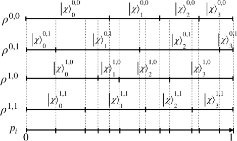
Figure 3: Given mixed states $\rho^{0,0}$, $\rho^{0,1}$, $\rho^{1,0}$ and $\rho^{1,1}$, each of which has it’s probabilistic mixture into pure states $\left|\chi^{x,y}_{i}\right\rangle$ displayed along a horizontal line with the distance between vertical markers representing $p^{x,y}_{i}$, we show in the bottom line probabilities $p_{i}$ for each of which all the $\rho^{x,y}$ mixtures have a fixed pure state.

Thus we can create any C-Q box outputting mixed states of 2 maximally disordered qubits.

VI Multi-Partite States

C-Q boxes with multi-partite states are more difficult to classify than bi-partite states, due to more parties being involved and the complexity of multi-partite entanglement. On the other hand, the no-signalling condition leads to many constraints on the sets of states which are allowed. In particular, we must not only have that there is no-signalling from $A$ to $B$, but also that there is no-signalling from $A$ to the joint system $BC$, and in general from any party to any other set of parties. Therefore even before asking whether a multi-partite C-Q box is genuine or not, even constructing a box while making sure it is non-signalling, is an issue in itself.

What we will show now, using a particular example, is that in some cases the non-signalling constraints are so strong that not only is the C-Q box non-genuine but it is LOSE, that is it can be implemented using $\bf{L}$ocal $\bf{O}$perations (i.e. unitaries) and pre-$\bf{S}$hared $\bf{E}$ntanglement, where the local operations only depend upon the local inputs. It does not require any other C-C box for correlating the local operations.

For our example we consider constructing a C-Q box whose outputs are $\left|W\right\rangle$ type states which differ by arbitrary phases in the computational basis, i.e.

$$\begin{split}&\left|\Psi^{x,y,z}\right\rangle_{ABC}=\\ &\frac{1}{\sqrt{3}}\left(e^{i\alpha(x,y,z)}\left|100\right\rangle+e^{i\beta(x,y,z)}\left|010\right\rangle+e^{i\gamma(x,y,z)}\left|001\right\rangle\right).\end{split}$$ (34)

This tri-partite “W-phase” C-Q box seems similar to the bi-partite phase boxes considered earlier. Yet, while the bi-partite C-Q box allows for correlated phases, we shall show that the only such non-signalling W-phase C-Q boxes are those whose phases are equivalent to local phases:

$$\frac{1}{\sqrt{3}}\left(e^{i\alpha(x)}\left|100\right\rangle+e^{i\beta(y)}\left|010\right\rangle+e^{i\gamma(z)}\left|001\right\rangle\right).$$ (35)

To prove this we will create the most general no-signalling box based on $\left|W\right\rangle$ with phases by using a no-signalling argument line by line in the following table.

$\begin{array}[]{c || c @{} c c c @{} c c c @{} c}\hline\cr xyz&&&&&&&\\ \hline\cr\hline\cr 000&&\left|100\right\rangle&+&&\left|010\right\rangle&+&&\left|001\right\rangle\\ \hline\cr 001&&\left|100\right\rangle&+&&\left|010\right\rangle&+&e^{i\gamma}&\left|001\right\rangle\\ \hline\cr 010&&\left|100\right\rangle&+&e^{i\beta}&\left|010\right\rangle&+&&\left|001\right\rangle\\ \hline\cr 100&e^{i\alpha}&\left|100\right\rangle&+&&\left|010\right\rangle&+&&\left|001\right\rangle\\ \hline\cr 011&&\left|100\right\rangle&+&e^{i\beta}&\left|010\right\rangle&+&e^{i\gamma}&\left|001\right\rangle\\ \hline\cr 101&e^{i\alpha}&\left|100\right\rangle&+&&\left|010\right\rangle&+&e^{i\gamma}&\left|001\right\rangle\\ \hline\cr 110&e^{i\alpha}&\left|100\right\rangle&+&e^{i\beta}&\left|010\right\rangle&+&&\left|001\right\rangle\\ \hline\cr 111&e^{i\alpha}&\left|100\right\rangle&+&e^{i\beta}&\left|010\right\rangle&+&e^{i\gamma}&\left|001\right\rangle\\ \hline\cr\end{array}$

In the first line, $\left|\Psi^{0,0,0}\right\rangle_{ABC}$ can be taken without loss of generality to be equal to the $\left|W\right\rangle$ state. The second line, $\left|\Psi^{0,0,1}\right\rangle_{ABC}$, is the output corresponding to a change of the input of C only. Hence, when we group A and B together, the reduced density matrix of AB must be the same for $\left|\Psi^{0,0,0}\right\rangle_{ABC}$ and $\left|\Psi^{0,0,1}\right\rangle_{ABC}$. The state $\left|\Psi^{0,0,0}\right\rangle_{ABC}$ can be written as

$$\left|\Psi^{0,0,0}\right\rangle_{ABC}=\frac{1}{\sqrt{3}}(\left|10\right\rangle_{AB}+\left|01\right\rangle_{AB})\left|0\right\rangle_{C}+\frac{1}{\sqrt{3}}\left|00\right\rangle_{AB}\left|1\right\rangle_{C}.$$ (36)

If change the relative phase between $\left|100\right\rangle$ and $\left|010\right\rangle$ it will change the density matrix $\rho_{AB}$ and hence be observable. So by no-signalling the only phase change we can make (up to an overall phase) between $\left|\Psi^{0,0,0}\right\rangle_{ABC}$ and $\left|\Psi^{0,0,1}\right\rangle_{ABC}$ is on $\left|001\right\rangle$. We call this phase factor $e^{i\gamma}$. Continuing in a similar way, we see that the only non-signalling W-phase box is (up to overall phases) the one in the above table.

Now the phases in the table are all local ($\alpha$ is present exactly when $x=1$, $\beta$ when $y=1$ etc). So not only are the W-phase C-Q boxes non-genuine, they are LOSE i.e they need no non-local C-C box if we want to create them in a non-genuine way. They can be implemented by local unitaries acting on pre-shared W states.

VII Conclusion

We have considered the issue of non-locality beyond quantum mechanics, and have introduced the concept of Classical input - Quantum output (C-Q) non-signalling boxes. We have investigated the question of whether such boxes are genuine new objects, or all of them could be constructed by objects already known, such as non-local non-signalling classical input - classical output boxes and pre-shared quantum entangled states. We have not been able to fully solve the problem but our study showed that some large class of C-Q boxes, including most bi-partite boxes outputting pure states with arbitrary dimensional inputs are non-genuine.

As far as multi-partite C-Q boxes outputting pure states are concerned, we conjecture that they are also non-genuine, similar to the bipartite ones. However while for some of them, such as the GHZ type phase boxes, the constraints are not much stronger than the bi-partite case, we conjecture that for the majority of the multi-partite states the constraints are so strong that they are LOSE in the same sense as the W-phase example.

There are a few more questions that follow immediately.

The first question concerns the use of resources when C-Q boxes can be be constructed from a C-C box and unitaries acting on pre-shared entanglement. We have shown that even when the C-Q box seems relatively simple, the C-C box needed for its simulation has to have a significant amount of non-locality. Moreover, even small changes to the C-Q box could result in major changes in the non-locality of the C-C needed (see the phase change box considered in sections III-C and III-D). One could presume that this is simply due to the fact that the output of the C-Q box, which is a quantum state, is in some sense “analog” (allows for phases that are given by real numbers), while the C-C box has a discrete number of outcomes, so more outcomes are necessary for simulating the continuous parameters in the definition of the quantum states. The problem, however, is not so simple, since in addition to the C-C box there are also the unitary transformations that are applied to the pre-shared quantum state, and unitaries are analog objects. Yet they are not enough. We found this behavious in a particular case, but expect it to be generic.

Second, and most important: What is the class of non-signalling C-Q boxes? We have encountered this problem when we attempted to decide whether all C-Q tri-partite boxes with pure-states outputs are are genuine or not. But how can we know that we considered all possible such boxes? If we call the set of output states of a non-signalling C-Q box a “non-signalling” set of quantum states, how can we find all such sets? That is, the nonsignaling condition (1) is very clear, and if we are given a set of states we can easily check if they fulfil it. But how to construct such a general set? What is its general structure? Crucially, the condition does not refer to the structure of each of the individual states separately but on the set as a whole. When dealing with multi-partite mixed states the problem is likely to be very difficult.

Incidentally, we also note that there are a few other, and quite important, examples of sets of states whose nonlocal properties are defined globally. For example, a set of orthogonal direct product states that cannot be reliable identified by local measurements and classical communication quantum nonlocality without entanglement . Another is that of states of two non-identical spin ½ particles used to indicate a direction in a 3D space. When dealing with a single direction, a state in which the two spins are parallel and pointing in the desired direction, is as good of indicating that direction as a state in which the spins are anti-parallel, with the first pointing in the desired direction and the second pointing opposite. But if we want to indicate many different directions, the set of anti-parallel spins is better than the set of parallel spins anti-parallel . This type of problems has only received relative little attention; we believe this to be a very important general problem for understanding the structure of quantum mechanics.

We believe the above are just the tip of an iceberg, and that considering C-Q boxes will lead to further insights into the issue of non-locality.

VIII Acknowledgements

We thank Paul Skrzypczyk for helpful discussions. Sandu Popescu and Daniel Collins acknowledge support of the ERC Advanced Grant FLQuant.

Note Added After completing this work we became aware of two related works we would like to mention. Firstly, D. Beckman, D. Gottesman, M. A. Nielsen, and J. Preskill causalLocalizableOperations considered the simple non-local C-Q Box we discuss in section III.1 in their section VI B, in the context of looking at quantum to quantum channels. Secondly D. Schmid, H. Du, M. Mudassar, G. Coulter-de Wit, D. Rosset, and M. J. Hoban postQuantumChannels discuss C-Q boxes as a part of classifying all non-signalling bi-partite boxes which have one of (classical, quantum, or empty) for each input/output on each side (e.g. classical input and classical output on side A, empty input and quantum output on side B). They also raised the question whether ”genuine” C-Q boxes exist (their ”open Question 2”), and showed that the C-Q box of section III.1 is equivalent to a PR box.

Appendix A State invariance under ${\hat{U}}_{A}{\hat{U}}_{B}^{*}$

Here we prove that

$${\hat{U}}_{A}{\hat{U}}^{*}_{B}\frac{1}{\sqrt{n}}\sum_{i}\left|i\right\rangle_{A}\left|i\right\rangle_{B}=\frac{1}{\sqrt{n}}\sum_{i}\left|i\right\rangle_{A}\left|i\right\rangle_{B},$$ (37)

where $n$ is the number of states $i$. Below $U_{i,j}$ is the $i,j$ matrix element of $U$, and we have dropped the normalization constant $\frac{1}{\sqrt{n}}$.

$$\begin{split}{\hat{U}}_{A}{\hat{U}}^{*}_{B}\sum_{i}\left|i\right\rangle_{A}\left|i\right\rangle_{B}&=\sum_{i}{\hat{U}}_{A}\left|i\right\rangle_{A}{\hat{U}}^{*}_{B}\left|i\right\rangle_{B}\\ &=\sum_{i}(\sum_{j}{\hat{U}}_{ji}\left|j\right\rangle_{A}\sum_{k}{\hat{U}}^{*}_{ki}\left|k\right\rangle_{B})\\ &=\sum_{jk}(\sum_{i}{\hat{U}}_{ji}{\hat{U}}^{*}_{ki})\left|j\right\rangle_{A}\left|k\right\rangle_{B}\\ &=\sum_{jk}({\hat{U}}{\hat{U}}^{\dagger})_{jk}\left|j\right\rangle_{A}\left|k\right\rangle_{B}\\ &=\sum_{jk}\mathbb{1}_{jk}\left|j\right\rangle_{A}\left|k\right\rangle_{B}\\ &=\sum_{k}\left|k\right\rangle_{A}\left|k\right\rangle_{B},\end{split}$$ (38)

as desired.

References

- (1) A. Einstein, B. Podolsky, and N. Rosen, Can quantum-mechanical description of physical reality be considered complete?, Phys. Rev. 47, 777–780 (1935).
- (2) J. S. Bell, On the Einstein Podolsky Rosen paradox, Physics 1,195–200(1964).
- (3) J.F. Clauser, M.A. Horne, A. Shimony and R.A. Holt, Phys. Rev. Lett. 23, 880 (1969)
- (4) S.J. Freedman and J.F. Clauser, Phys. Rev. Lett. 28, 938 (1972)
- (5) A. Aspect, P.Grangier and G.Roger, Phys. Rev. Lett. 47, 460 (1981).
- (6) B. S. Cirel’son (1980). Quantum generalizations of Bell’s inequality. Letters in Mathematical Physics. 4 (2): 93–100.
- (7) S. Popescu and D. Rohrlich, it Quantum nonlocality as an axiom, Found. Phys. 24, 379–385 (1994).
- (8) J. Barrett, N. Linden, S. Massar, S. Pironio, S. Popescu, and D. Roberts, Nonlocal correlations as an information- theoretic resource, Phys. Rev. A 71, 10.1103/phys-reva.71.022101 (2005).
- (9) P. Skrzypczyk, N. Brunner, and S. Popescu, Emergence of quantum correlations from nonlocality swapping, Phys. Rev. Lett. 102, 10.1103/physrevlett.102.110402 (2009).
- (10) M. Pawlowski, T. Paterek, D. Kaszlikowski, V. Scarani, A.Winter and M.Zukowski, Information causality as a physical principle, Nature 461, 1101–1104 (2009).
- (11) N. Linden, S. Popescu, A. J. Short, and A. Winter, Quantum nonlocality and beyond: Limits from non- local computation, Phys. Rev. Lett. 99, 10.1103/phys-revlett.99.180502 (2007).
- (12) W. van Dam Implausible consequences of superstrong nonlocality. quant-ph/0501159 (2005).
- (13) G. Brassard, H. Buhrman, N. Linden, A. A. Méthot, A. Tapp, and F. Unger, Limit on Nonlocality in Any World in Which Communication Complexity Is Not Trivial Phys. Rev. Lett. 96, 250401 (2006)
- (14) A. J. Short, S. Popescu, and N. Gisin Entanglement swapping for generalized nonlocal correlations, Phys. Rev. A 73, 012101 (2006)
- (15) J. Barrett and A. J. Short Strong non-locality: a tradeoff between states and measurements, New J. Phys. 12, 33034 (2010).
- (16) R. Horodecki and M. Horodecki, Information-theoretic aspects of quantum inseparability of mixed states, Phys. Rev. A 54, (1996).
- (17) C. H. Bennett,et al. Quantum nonlocality without entanglement, Phys. Rev. A 59, 1070 (1999).
- (18) N. Gisin and S. Popescu, Spin Flips and Quantum Information for Antiparallel Spins, Phys. Rev. Lett. 83, p. 432 (1999).
- (19) D. Beckman, D. Gottesman, M. A. Nielsen, and J. Preskill, Causal and localizable quantum operations Phys. Rev. A 64, 052309 (2001)
- (20) D. Schmid, H. Du, M. Mudassar, G. Coulter-de Wit, D. Rosset, and M. J. Hoban, Postquantum common-cause channels: the resource theory of local operations and shared entanglement, Quantum 5, 419 (2021)