Coskewness under dependence uncertainty

Abstract

We study the impact of dependence uncertainty on $\mathbb{E}(X_{1}X_{2}\cdots X_{d})$ when $X_{i}\sim F_{i}$ for all $i$. Under some conditions on the $F_{i}$, explicit sharp bounds are obtained and a numerical method is provided to approximate them for arbitrary choices of the $F_{i}$. The results are applied to assess the impact of dependence uncertainty on coskewness. In this regard, we introduce a novel notion of “standardized rank coskewness,” which is invariant under strictly increasing transformations and takes values in $[-1,\ 1]$.

Keywords: Expected product, Higher-order moments, Copula, Coskewness, Risk bounds.

1 Introduction

A fundamental characteristic of a multivariate random vector $\left(X_{1},X_{2},\dots,X_{d}\right)$ concerns the k-th order mixed moment

$$\mathbb{E}\left(X_{1}^{k_{1}}X_{2}^{k_{2}}\cdots X_{d}^{k_{d}}\right)=\int_{\mathbb{R}^{d}}x_{1}^{k_{1}}x_{2}^{k_{2}}\cdots x_{d}^{k_{d}}dF(x_{1},x_{2},\dots,x_{d}),$$

where $k_{i},$ $i=1,2,\dots,d,$ are non-negative integers such that $\sum_{i=1}^{d}k_{i}=k$ and $F$ is the joint distribution function of $\left(X_{1},X_{2},\dots,X_{d}\right)$; see e.g., Kotz et al. (2004). A classic problem in multivariate modeling is to find sharp bounds on mixed moments under the assumption that the marginal distribution functions of the $X_{i}$ are known but not their dependence. The solutions in case $d=2$ are well-known but for higher dimensions a complete solution is still missing. In this regard, it is well-known that under the assumption that all $X_{i}$ are non-negative, the sharp upper bound is obtained in case the variables have a comonotonic dependence. As for the lower bound problem, Wang and Wang (2011) obtain a sharp bound under the assumption that the $X_{i}$ are standard uniformly distributed. To the best of our knowledge, there are no other relevant results available in the literature.

In the first part of this paper, we determine for the case $k_{i}=1$ $(i=1,2,\dots,d)$ sharp lower and upper bounds on mixed moments under some assumptions on the marginal distribution functions of $X_{i}$. When $k_{i}\neq 1$ and the domain of marginal distributions is non-negative, these bounds are also solvable under a mixing assumption on the distributions of $k_{i}\ln X_{i}$. Furthermore, we establish a necessary condition that solutions to the optimization problems need to satisfy and use this result to design an algorithm that approximates the sharp bounds.

A special case of finding bounds on mixed moments concerns the case of standardized central mixed moments, such as covariance (second-order), coskewness (third-order) and cokurtosis (fourth-order). The sharp lower and upper bounds in the case of covariance are very well-known in the literature, and in the second part of the paper we focus on the application of our results to obtaining bounds on coskewness. We obtain explicit risk bounds for some popular families of marginal distributions, such as uniform, normal and Student’s t distributions. Furthermore, we introduce the novel notion of standardized rank coskewness and discuss its properties. Specifically, as the standardized rank coskewness takes values in $[-1,\ 1]$ and is not affected by the choice of marginal distributions, this notion makes it possible to interpret the sign and magnitude of coskewness without impact of marginal distributions. In spirit, the standardized rank coskewness extends the notion of Spearman’s correlation coefficient to three dimensions.

The paper is organized as follows. In Section 2, we lay out the optimization problem. In Section 3, we derive sharp bounds under various conditions on the marginal distribution functions and also provide a numerical approach to approximate the sharp bounds in general. We apply our results in Section 4 to introduce the notion of standardized rank coskewness.

2 Problem setting

In what follows all random variables $X_{i}\sim F_{i}$, $i=1,2,\dots,d$, that we consider are assumed to be square integrable. We denote their means and standard deviations by $\mu_{i}$ and $\sigma_{i}$, respectively. Furthermore, $U$ always denotes a standard uniform distributed random variable. The central question of this paper is to derive lower and upper bounds on the expectation of the product of $d\geq 2$ random variables under dependence uncertainty. Specifically, we consider the problems

$$m =\inf\limits_{\forall i\ X_{i}\sim F_{i}}\mathbb{E}\left(X_{1}X_{2}\cdots X_{d}\right);$$ (2.1)

$$M =\sup\limits_{\forall i\ X_{i}\sim F_{i}}\mathbb{E}\left(X_{1}X_{2}\cdots X_{d}\right).$$ (2.2)

When $d=2$, it is well-known that $M$ is given by $\mathbb{E}(F_{1}^{-1}(U)F_{2}^{-1}(U))$ (comonotonicity), and $m$ is given by $\mathbb{E}(F_{1}^{-1}(U)F_{2}^{-1}(1-U))$ (antimonotonicity). For general $d$, the lower bound problem has a long history when $X_{i}\sim U[0,1]$, (see e.g., Rüschendorf, 1980; Bertino, 1994; Nelsen and Úbeda-Flores, 2012). Specifically, Wang and Wang (2011) found the following closed-form expression (Corollary 4.1) for $m$ in the case of $X_{i}\sim U[0,1]$:

$$m=\frac{1}{(d-1)^{2}}\left(\frac{1}{d+1}-(1-(d-1)c_{d})^{d}+\frac{d}{d+1}(1-(d-1)c_{d})^{d+1}\right)+(1-dc_{d})c_{d}(1-(d-1)c_{d})^{d-1},$$ (2.3)

where $c_{d}$ is the unique solution to $\log\left(1-d+\frac{1}{c}\right)=d-d^{2}c.$ Clearly, for $M$ we find in this case that $M=\mathbb{E}(U^{d})=\frac{1}{d+1}$. When $X_{i}\sim U[a,b]$ such that $0<a<b<\infty$ and the inequality $\exp\{\frac{d}{b-a}(b(\ln b-1)-a(\ln a-1))\}-ab^{d-1}\leq 0$ holds, Bignozzi and Puccetti (2015) found the analytic result $m=\left(\frac{b^{b}e^{a}}{a^{a}e^{b}}\right)^{\frac{d}{b-a}}$.

However, as far as we know, there are no other results available in the literature for computing $m$ and $M$ in more general cases. In the following section, we contribute to the literature by solving explicitly Problems (2.1) and (2.2) under various assumptions on the marginal distributions $F_{i}$, $i=1,2,\dots,d$ (Section 3.1), or via an algorithm for arbitrary choices of $F_{i}$ (Section 3.2).

3 Lower and upper bounds

3.1 Analytic results

We first provide lower and upper bounds when the $F_{i}$ are symmetric and have zero means. Next we study the case in which the $F_{i}$ satisfy some domain constraints or when they are uniform distributions on $(a,b)$, $a<0<b$. Our results make use of the following two lemmas.

Lemma 3.1 (Maximum product).

Let $X_{i}\sim F_{i}$, denote by $G_{i}$ the df of the absolute value of $X_{i}$ $($i.e., $\lvert X_{i}\rvert\sim G_{i}$$)$, $i=1,2,\dots,d,$ and $U\sim U[0,1]$. Then,

$$M\leq\mathbb{E}\left(\prod_{i=1}^{d}G_{i}^{-1}(U)\right).$$ (3.1)

If $\lvert X_{1}\rvert$, $\lvert X_{2}\rvert$, $\dots$, $\lvert X_{d}\rvert$ are comonotonic and $\prod_{i=1}^{d}X_{i}\geq 0$ a.s., then $(X_{1},X_{2},\dots,X_{d})$ attains the maximum value $M$ and equality holds in (3.1).

Proof.

As for the first part of the lemma, note that for any random vector $(Y_{1},Y_{2},\dots,Y_{d})$ such that $Y_{i}\sim F_{i},$ $i=1,2,\dots,d,$ it holds that $\mathbb{E}(\prod_{i=1}^{d}Y_{i})\leq\mathbb{E}(\prod_{i=1}^{d}\lvert Y_{i}\rvert).$ (3.1) then follows from the well-known fact that the right hand side of this inequality is maximized under a comonotonic dependence among the $\mathinner{\!\left\lvert Y_{i}\right\rvert}$. As for the second part, since $\lvert X_{i}\rvert\overset{d}{=}\lvert Y_{i}\rvert,$ the $\mathinner{\!\left\lvert X_{i}\right\rvert}$ are comonotonic, and $\prod_{i=1}^{d}X_{i}\geq 0,$ it follows that $\mathbb{E}(\prod_{i=1}^{d}Y_{i})\leq\mathbb{E}(\prod_{i=1}^{d}\lvert X_{i}\rvert)=\mathbb{E}(\prod_{i=1}^{d}X_{i}).$ ∎

Lemma 3.2 (Minimum product).

Let $X_{i}\sim F_{i}$, denote by $G_{i}$ the df of the absolute value of $X_{i}$ $($i.e., $\lvert X_{i}\rvert\sim G_{i}$$)$, $i=1,2,\dots,d,$ and $U\sim U[0,1]$. Then,

$$m\geq-\mathbb{E}\left(\prod_{i=1}^{d}G_{i}^{-1}(U)\right).$$ (3.2)

If $\lvert X_{1}\rvert$, $\lvert X_{2}\rvert$, $\dots$, $\lvert X_{d}\rvert$ are comonotonic and $\prod_{i=1}^{d}X_{i}\leq 0$ a.s., then $(X_{1},X_{2},\dots,X_{d})$ attains the minimum value $m$ and equality holds in (3.2).

Proof.

The proof is similar to the proof of the previous lemma noting that $\mathbb{E}(\prod_{i=1}^{d}X_{i})=-\mathbb{E}(\prod_{i=1}^{d}\lvert X_{i}\rvert)$ when $\prod_{i=1}^{d}X_{i}\leq 0$ a.s.. ∎

3.1.1 Symmetric marginal distributions

The following two theorems are main contributions of this paper.

Theorem 3.1 (Upper bound).

Let $F_{i}$, $i=1,2,\dots,d$, be symmetric with zero means and $U\sim U[0,1]$. There exists a random vector $(X_{1},X_{2},\dots,X_{d})$ such that the $\lvert X_{1}\rvert$, $\lvert X_{2}\rvert$, $\dots$, $\lvert X_{d}\rvert$ are comonotonic and $\prod_{i=1}^{d}X_{i}\geq 0$ a.s.. Hence, $M=\mathbb{E}(\prod_{i=1}^{d}G_{i}^{-1}(U))$ where $G_{i}$ denotes the df of $\lvert X_{i}\rvert$. Furthermore, if $d$ is odd, then $X_{i}=F_{i}^{-1}(U_{i})$ with

$$U_{1} =U_{2}=\cdots=U_{d-2}=U,$$ (3.3)

$$U_{d-1} =IJU+I(1-J)(1-U)+(1-I)JU+(1-I)(1-J)(1-U),$$

$$U_{d} =IJU+I(1-J)(1-U)+(1-I)J(1-U)+(1-I)(1-J)U,$$

where $I=\mathds{1}_{U>\frac{1}{2}}$, $J=\mathds{1}_{V>\frac{1}{2}}$, and $V\overset{d}{=}U[0,1]$ is independent of $U$. If $d$ is even, then $X_{i}=F_{i}^{-1}(U_{i})$ with

$$U_{1}=U_{2}=\cdots=U_{d}=U.$$ (3.4)

Proof.

(1) $d$ is odd. The random variables $X_{j}$, $j=1,2,\dots,d-2$, can be expressed as follows:

$$X_{j}=IJF^{-1}_{j}(U)+I(1-J)F^{-1}_{j}(U)+(1-I)JF^{-1}_{j}(U)+(1-I)(1-J)F^{-1}_{j}(U).$$

Furthermore,

$$X_{d-1} =IJF^{-1}_{d-1}(U)+I(1-J)F^{-1}_{d-1}(1-U)+(1-I)JF^{-1}_{d-1}(U)+(1-I)(1-J)F^{-1}_{d-1}(1-U),$$

$$X_{d} =IJF^{-1}_{d}(U)+I(1-J)F^{-1}_{d}(1-U)+(1-I)JF^{-1}_{d}(1-U)+(1-I)(1-J)F^{-1}_{d}(U).$$

It follows that

$$\mathinner{\!\left\lvert X_{j}\right\rvert} =IJF^{-1}_{j}(U)+I(1-J)F^{-1}_{j}(U)-(1-I)JF^{-1}_{j}(U)-(1-I)(1-J)F^{-1}_{j}(U)$$

$$=IF^{-1}_{j}(U)-(1-I)F^{-1}_{j}(U),$$

$$\mathinner{\!\left\lvert X_{d-1}\right\rvert} =IJF^{-1}_{d-1}(U)-I(1-J)F^{-1}_{d-1}(1-U)-(1-I)JF^{-1}_{d-1}(U)+(1-I)(1-J)F^{-1}_{d-1}(1-U)$$

$$=IJF^{-1}_{d-1}(U)+I(1-J)F^{-1}_{d-1}(U)-(1-I)JF^{-1}_{d-1}(U)-(1-I)(1-J)F^{-1}_{d-1}(U)$$

$$=IF^{-1}_{d-1}(U)-(1-I)F^{-1}_{d-1}(U),$$

$$\mathinner{\!\left\lvert X_{d}\right\rvert} =IJF^{-1}_{d}(U)-I(1-J)F^{-1}_{d}(1-U)+(1-I)JF^{-1}_{d}(1-U)-(1-I)(1-J)F^{-1}_{d}(U)$$

$$=IJF^{-1}_{d}(U)+I(1-J)F^{-1}_{d}(U)-(1-I)JF^{-1}_{d}(U)-(1-I)(1-J)F^{-1}_{d}(U)$$

$$=IF^{-1}_{d}(U)-(1-I)F^{-1}_{d}(U),$$

where we used in the second equations for $\mathinner{\!\left\lvert X_{d-1}\right\rvert}$ and $\mathinner{\!\left\lvert X_{d}\right\rvert}$ that $F_{d-1}$ resp. $F_{d}$ is symmetric. Note that the $\lvert X_{i}\rvert$ also write as $\lvert X_{i}\rvert=F_{i}^{-1}(Z)$, $i=1,2,\dots,d$, where $Z=U$ if $U\geq\frac{1}{2}$ and $Z=1-U$ if $U<\frac{1}{2}$, i.e., $Z=\frac{1}{2}+\lvert U-\frac{1}{2}\rvert$. Next, we show that $\lvert X_{1}\rvert,\lvert X_{2}\rvert,\dots,\lvert X_{d}\rvert$ are comonotonic and that $\prod_{i=1}^{d}X_{i}\geq 0$ a.s.. First, $\lvert X_{i}\rvert$, $i=1,2,\dots,d$, are comonotonic because they are all increasing functions of $\lvert U-\frac{1}{2}\rvert$. Second,

$$\prod_{i=1}^{d}X_{i}= IJ\prod_{i=1}^{d}F^{-1}_{i}(U)+I(1-J)F^{-1}_{d-1}(1-U)F^{-1}_{d}(1-U)\prod_{i=1}^{d-2}F^{-1}_{i}(U)+$$

$$(1-I)J\prod_{i=1}^{d-1}F^{-1}_{i}(U)F^{-1}_{d}(1-U)+(1-I)(1-J)F^{-1}_{d-1}(1-U)F^{-1}_{d}(U)\prod_{i=1}^{d-2}F^{-1}_{1}(U),$$

which is greater than or equal to zero because $F^{-1}_{i}(U)>0$ and $F^{-1}_{i}(1-U)\leq 0$ when $U>\frac{1}{2}$, and $F^{-1}_{i}(U)\leq 0$ and $F^{-1}_{i}(1-U)>0$ when $U\leq\frac{1}{2}$, and where we use that $d$ is odd. Therefore, the vector $(X_{1},X_{2},\dots,X_{d})$ with $X_{i}=F_{i}^{-1}(U_{i})$, in which the $U_{i}$ are given as in (3.3), attains $M$.

(2) $d$ is even. The random variables $X_{i}$ can be expressed as $X_{i}=IF^{-1}_{i}(U)+(1-I)F^{-1}_{i}(U)$. Hence, $\lvert X_{i}\rvert=IF^{-1}_{i}(U)-(1-I)F^{-1}_{i}(U)$. It is clear that $\lvert X_{1}\rvert,\lvert X_{2}\rvert,\dots,\lvert X_{d}\rvert$ are comonotonic, as they are all increasing in $\lvert U-\frac{1}{2}\rvert$. Furthermore, $\prod_{i=1}^{d}X_{i}=I\prod_{i=1}^{d}F^{-1}_{i}(U)+(1-I)\prod_{i=1}^{d}F^{-1}_{i}(U),$ which is greater than or equal to zero (note that $d$ is even). Therefore, the random vector $(X_{1},X_{2},\dots,X_{d})$ with $X_{i}=F_{i}^{-1}(U)$ attains $M$. ∎

Theorem 3.2 (Lower bound).

Let $F_{i}$, $i=1,2,\dots,d$, be symmetric with zero means and $U\sim U[0,1]$. There exists a random vector $(X_{1},X_{2},\dots,X_{d})$ such that $\lvert X_{1}\rvert$, $\lvert X_{2}\rvert$, $\dots$, $\lvert X_{d}\rvert$ are comonotonic and $\prod_{i=1}^{d}X_{i}\leq 0$ a.s.. Hence, $m=-\mathbb{E}(\prod_{i=1}^{d}G_{i}^{-1}(U))$ where $G_{i}$ is the df of $\lvert X_{i}\rvert$. Furthermore, if $d$ is odd, then $X_{i}=F_{i}^{-1}(U_{i})$ with

$$U_{1} =U_{2}=\cdots=U_{d-2}=U,$$ (3.5)

$$U_{d-1} =IJU+I(1-J)(1-U)+(1-I)JU+(1-I)(1-J)(1-U),$$

$$U_{d} =IJ(1-U)+I(1-J)U+(1-I)JU+(1-I)(1-J)(1-U),$$

where $I=\mathds{1}_{U>\frac{1}{2}}$, $J=\mathds{1}_{V>\frac{1}{2}}$, and $V\overset{d}{=}U[0,1]$ is independent of $U$. If $d$ is even, then $X_{i}=F_{i}^{-1}(U_{i})$ with

$$U_{1} =U_{2}=\cdots=U_{d-1}=U\quad\hbox{and}\quad U_{d}=1-U.$$ (3.6)

We omit the proof of the lower bound because it is similar to that of the upper bound. Figure 1 presents the supports of the copulas in (3.3) and (3.5) when $d=3$. As the projections of the support on the planes formed by the x-axis and y-axis, resp. x-axis and z-axis, resp. y-axis and z-axis form crosses, we label these copulas as cross product copulas. Note that the simulation shows the densities of the cross product copulas are uniform on each of the segments.

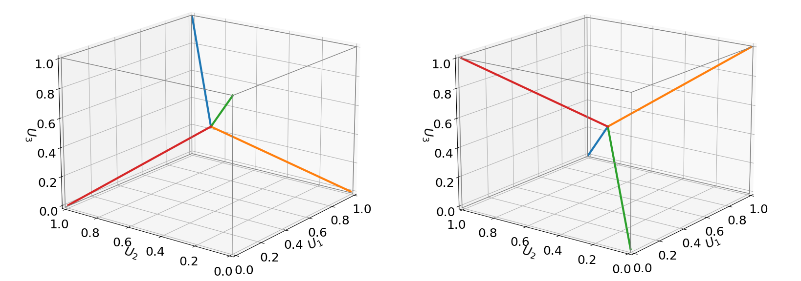
Figure 1: Support of the (cross product) copula that maximizes (left panel) resp. minimizes (right panel) $\mathbb{E}(X_{1}X_{2}X_{3})$ where $X_{i}\sim F_{i}$ ($i=1,2,3$) in the case that the $F_{i}$ are symmetric with zero means.

Corollary 3.1.

Let the $F_{i}$ be uniform distributions on $\left[-\sqrt{3},\sqrt{3}\right]$. Then $M=\left(\sqrt{3}\right)^{d}/(d+1)$ and is attained by a random vector $(X_{1},X_{2},\dots,X_{d})$, where $X_{i}=F_{i}^{-1}(U_{i})$ in which the $U_{i}$ are given in (3.3) $($resp., (3.4)$)$ if $d$ is odd $($resp., even$)$. Furthermore, $m=-\left(\sqrt{3}\right)^{d}/(d+1)$ and is attained by a random vector $(X_{1},X_{2},\dots,X_{d})$ where $X_{i}=F_{i}^{-1}(U_{i})$ in which the $U_{i}$ are given in (3.5) $($resp., (3.6)$)$ if $d$ is odd $($resp., even$)$.

Proof.

With $X_{i}\sim\left[-\sqrt{3},\sqrt{3}\right]$, we find that $|X_{i}|\mathrel{\mathop{\mathchar 58\relax}}=V\sim U\left[0,\sqrt{3}\right]$. Then we find from Theorem 3.1 that $M=\mathbb{E}(V^{d})=\int_{0}^{\sqrt{3}}v^{d}\frac{\sqrt{3}}{3}dv=\frac{3^{\frac{d}{2}}}{d+1}.$ In a similar way, we find from Theorem 3.2 that $m=-3^{\frac{d}{2}}/(d+1)$. ∎

Remark 3.1.

For general distribution functions $F_{i}$, $i=1,2,\dots,d$, the upper bound in (3.1) and the lower bound in (3.2) are typically not attainable. Moreover, the construction $X_{i}=F_{i}^{-1}(U_{i})$ with the $U_{i}$ as given in (3.3) ($d$ is odd) resp. as given in (3.4) ($d$ is even) does not lead to the sharp bound $M$ (similar for the case of the lower bound $m$). To illustrate this point, let the $F_{i}$, $i=1,2,3,$ denote discrete distributions having mass points -1 and 10 with equal probability. Under a comonotonic dependence among the $X_{i}\sim F_{i}$, we obtain that $\mathbb{E}\left(X_{1}X_{2}X_{3}\right)=499.5$. However, under the dependence as in (3.3), we obtain that $\mathbb{E}\left(X_{1}X_{2}X_{3}\right)=257.5<499.5$. Moreover, $\mathbb{E}\left(\lvert X_{1}\rvert\lvert X_{2}\rvert\lvert X_{3}\rvert\right)=500.5$ is not attainable.

3.1.2 Marginal distributions under domain restrictions

In this subsection, we provide sharp bounds under various conditions that the domain of $F_{i}$ is non-negative or non-positive, or that the $F_{i}$ are uniforms on $(a,b)$, $a<0<b$.

Proposition 3.1 (Non-negative domain).

Let $X_{i}\sim F_{i}$ in which the $F_{i}$ have non-negative domain.

1. The upper bound $M$ is attained when $(X_{1},X_{2},\dots,X_{d})$ is a comonotonic random vector, i.e., $X_{i}=F_{i}^{-1}(U)$ in which $U\sim U[0,1]$.

2. Under a mixing assumption on the distributions of $\ln X_{1},\ln X_{2},\dots,\ln X_{d}$, i.e., $\sum_{i=1}^{d}\ln X_{i}=c$, where $c$ is a constant, it holds that $m=e^{c}$ and $m$ is attained by $(X_{1},X_{2},\dots,X_{d})$.

Proof.

The first statement follows from Lemma 3.1 in a direct manner. As for the proof of the second statement, it holds for any $Y_{i}\sim F_{i}$, $i=1,2,\dots,d$ that $\mathbb{E}\left(\prod_{i=1}^{d}Y_{i}\right)=\mathbb{E}\left(\exp\left(\sum_{i=1}^{d}\ln Y_{i}\right)\right)\geq\exp\left(\mathbb{E}\left(\sum_{i=1}^{d}\ln Y_{i}\right)\right)$ where the last inequality follows from Jensen’s inequality. Furthermore, this inequality turns into an equality when $\sum_{i=1}^{d}\ln Y_{i}$ is constant. This implies the second statement. ∎

Remark 3.2.

For k-th order mixed moments and $X_{i}\sim F_{i}$ in which the $F_{i}$ have non-negative domains, $i=1,2,\dots,d$, we obtain from Proposition 3.1 the lower and upper bound of $\mathbb{E}\left(X_{1}^{k_{1}}X_{2}^{k_{2}}\cdots X_{d}^{k_{d}}\right)$. Under a mixing assumption on the distributions of $k_{1}\ln X_{1},k_{2}\ln X_{2},\dots,k_{d}\ln X_{d}$, it holds that the lower bound is attained by $(X_{1},X_{2},\dots,X_{d})$. The mixing conditions for this case are given in Section 3 of Wang and Wang (2016). In particular, this holds true in case $k_{1}=k_{2}=\cdots=k_{d}=l$ in which $l$ is an integer and $l\geq 1$, and the lower bound is $m^{l}$, where $m$ is the value in (2.3).

Proposition 3.2 (Non-positive domain).

Let $X_{i}\sim F_{i}$ in which the $F_{i}$ have non-positive domain and $U\sim U[0,1]$.

1. Let $d$ be an odd number. Under a mixing assumption on the distributions of $\ln\lvert X_{1}\rvert,\ln\lvert X_{2}\rvert,\dots,$ $\ln\lvert X_{d}\rvert$, i.e., $\sum_{i=1}^{d}\ln\lvert X_{i}\rvert=c$, where $c$ is a constant, it holds that $M=-e^{c}$ and $M$ is attained by $(X_{1},X_{2},\dots,X_{d})$. $m$ is attained when $(X_{1},X_{2},\dots,X_{d})$ is a comonotonic random vector, i.e., $X_{i}=F_{i}^{-1}(U)$.

2. Let $d$ be an even number. $M$ is attained when $(X_{1},X_{2},\dots,X_{d})$ is a comonotonic random vector, i.e., $X_{i}=F_{i}^{-1}(U)$. Under a mixing assumption on the distributions of $\ln\lvert X_{1}\rvert,\ln\lvert X_{2}\rvert,\dots,\ln\lvert X_{d}\rvert$, i.e., $\sum_{i=1}^{d}\ln\lvert X_{i}\rvert=c$, where $c$ is a constant, it holds that $m=e^{c}$ and $m$ is attained by $(X_{1},X_{2},\dots,X_{d})$.

Proof.

Its proof is similar to that of Proposition 3.1, we thus omit it. $\Box$

Proposition 3.2 shows that when the $F_{i}$ have non-positive domain and $d$ is odd, an upper bound on $M$ is given by $-\exp\left(\mathbb{E}\left(\sum_{i=1}^{d}\ln\lvert Y_{i}\rvert\right)\right)$, $Y_{i}\sim F_{i}$. Wang and Wang (2011, 2015), Puccetti and Wang (2015), and Puccetti et al. (2012) provide general conditions on the $F_{i}$ that ensure the construction of $X_{i}\sim F_{i}$ such that the distributions of $X_{1},X_{2},\dots,X_{d}$ are mixing and thus allow to infer sharpness of the bounds above. For early results of this type, see Gaffke and Rüschendorf (1981) and Rüschendorf and Uckelmann (2002).

Proposition 3.3 (Uniform distributions with non-zero means).

Let $X_{i}\sim F_{i}$, $i=1,2,\dots,d$. Assume that $d$ is odd and that the $F_{i}$ are uniform distributions on $[a,b]$ $(a<0<b).$ Define $J=\mathds{1}_{V>\frac{1}{2}}$, in which $V\sim U[0,1]$ is independent of $U\sim U[0,1]$. It holds that:

1. Let $\mathinner{\!\left\lvert a\right\rvert}<b$ and $c=\frac{-2a}{b-a}$. $M$ is attained by a random vector $(X_{1},X_{2},\dots,X_{d}),$ with $X_{i}=F_{i}^{-1}(U_{i})$ in which

   $$U_{1}= U_{2}=\cdots=U_{d-2}=U,$$ (3.7)

   $$U_{d-1}= (1-I)[KJU+K(1-J)(c-U)+(1-K)JU+(1-K)(1-J)(c-U)]+IU,$$

   $$U_{d}= (1-I)[KJU+K(1-J)(c-U)+(1-K)J(c-U)+(1-K)(1-J)U]+IU,$$

   and where $I=\mathds{1}_{U>c}$ and $K=\mathds{1}_{U>\frac{c}{2}}$.

2. Let $\mathinner{\!\left\lvert a\right\rvert}>b$ and $c=\frac{-b-a}{b-a}$. $m$ is attained by the random vector $(X_{1},X_{2},\dots,X_{d})$, with $X_{i}=F_{i}^{-1}(U_{i})$ in which

   $$U_{1}= U_{2}=\cdots=U_{d-2}=U,$$ (3.8)

   $$U_{d-1}= (1-I)[KJU+K(1-J)(1+c-U)+(1-K)JU+(1-K)(1-J)(1+c-U)]+IU,$$

   $$U_{d}= (1-I)[KJ(1+c-U)+K(1-J)U+(1-K)JU+(1-K)(1-J)(1+c-U)]+IU,$$

   and where $I=\mathds{1}_{U<c}$ and $K=\mathds{1}_{U>\frac{1+c}{2}}$.

Proof.

1. Note that $F_{i}^{-1}(u)>0$ if and only if $u>\frac{c}{2}$. When $1\leq j\leq d-2,$ $X_{j}=F^{-1}_{j}(U).$ Moreover,

   $$X_{d-1}= (1-I)[KJF^{-1}_{d-1}(U)+K(1-J)F^{-1}_{d-1}(c-U)+(1-K)JF^{-1}_{d-1}(U)$$

   $$+(1-K)(1-J)F^{-1}_{d-1}(c-U)]+IF^{-1}_{d-1}(U),$$

   $$X_{d}= (1-I)[KJF^{-1}_{d}(U)+K(1-J)F^{-1}_{d}(c-U)+(1-K)JF^{-1}_{d}(c-U)$$

   $$+(1-K)(1-J)F^{-1}_{d}(U)]+IF^{-1}_{d}(U).$$

   The absolute values of $X_{i}$ are

   $$\mathinner{\!\left\lvert X_{j}\right\rvert}= (1-I)[KF^{-1}_{j}(U)-(1-K)F^{-1}_{j}(U)]+IF^{-1}_{j}(U)$$

   $$\mathinner{\!\left\lvert X_{d-1}\right\rvert}= (1-I)[KJF^{-1}_{d-1}(U)-K(1-J)F^{-1}_{d-1}(c-U)-(1-K)JF^{-1}_{d-1}(U)$$

   $$+(1-K)(1-J)F^{-1}_{d-1}(c-U)]+IF^{-1}_{d-1}(U)$$

   $$= (1-I)[KF^{-1}_{d-1}(U)-(1-K)F^{-1}_{d-1}(U)]+IF^{-1}_{d-1}(U),$$

   $$\mathinner{\!\left\lvert X_{d}\right\rvert}= (1-I)[KJF^{-1}_{d}(U)-K(1-J)F^{-1}_{d}(c-U)+(1-K)JF^{-1}_{d}(c-U)$$

   $$-(1-K)(1-J)F^{-1}_{d}(U)]+IF^{-1}_{d}(U)$$

   $$= (1-I)[KF^{-1}_{d}(U)-(1-K)F^{-1}_{d}(U)]+IF^{-1}_{d}(U).$$

   The above equations for $\mathinner{\!\left\lvert X_{d-1}\right\rvert}$ and $\mathinner{\!\left\lvert X_{d}\right\rvert}$ hold because $-F^{-1}_{d}(c-U)=F^{-1}_{d}(U)$ if $U\leq c$. Similarly to Theorem 3.1, we apply Lemma 3.1 to prove this proposition. First, $\lvert X_{i}\rvert$, $i=1,2,\dots,d$, are comonotonic because they are all increasing functions of $\lvert U-\frac{c}{2}\rvert$ ($\lvert X_{i}\rvert=F^{-1}_{i}(Z)$ where $Z=\frac{c}{2}+\lvert U-\frac{c}{2}\rvert$). Moreover, it verifies that $\prod_{i=1}^{d}X_{i}\geq 0$ if $d$ is odd. Hence, $M$ is attained by the random vector $(X_{1},X_{2},\dots,X_{d})$, where $X_{i}=F_{i}^{-1}(U_{i})$ with $U_{i}$ in (3.7).

2. The proof of (2) is similar to that of (1) and thus omitted. $\Box$

Figure 2 displays the supports of the copulas in (3.7) and (3.8) when $d=3$ and $a<0$.

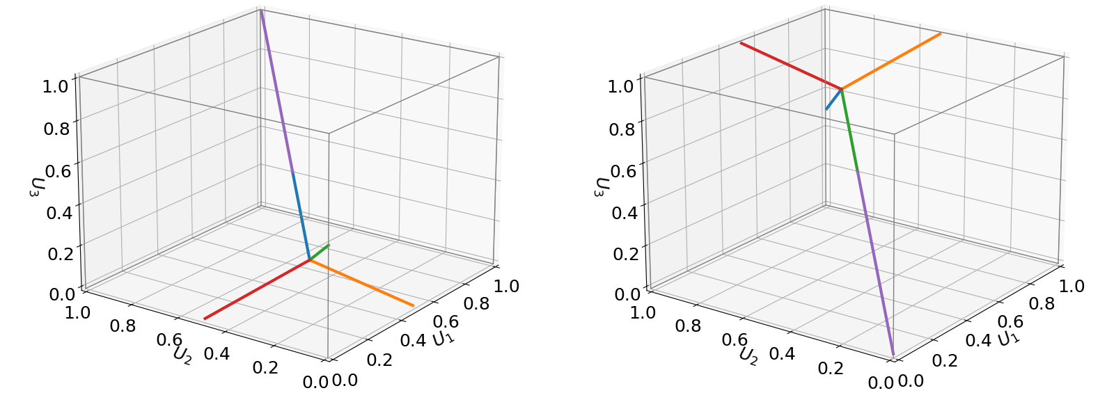
Figure 2: Support of the copula (3.7) (resp., (3.8)) that maximizes (left panel) (resp., minimizes (right panel)) $\mathbb{E}(X_{1}X_{2}X_{3})$ with $F_{i}\sim U[a,-3a]$ (resp., $F_{i}\sim U[a,-a/3]$), in which $a<0$ and $c=\frac{1}{2}$.

3.2 Algorithm for obtaining sharp bounds

In this subsection, we develop an algorithm to approximate for any given choice of $F_{i},$ $i=1,2,\dots,d$, the sharp bounds $m$ and $M$. The algorithm is based on the following lemma that establishes necessary conditions that the solutions to the optimization problems (2.2) resp. (2.1) need to satisfy.

Lemma 3.3.

If $(X_{1},X_{2},\dots,X_{d})$ solves problem (2.2) $($resp., (2.1)$)$, then for any choice of subsets $I$ of $\{1,2,\dots,d\}$, it holds that $X_{1}=\prod_{i\in I}X_{i}$ and $X_{2}=\prod_{i\notin I}X_{i}$ are comonotonic $($resp., antimonotonic$)$.

Making use of Lemma 3.3, we can now design an algorithm to obtain approximate solutions to problems (2.1) and (2.2).

Algorithm 3.1.

2. Simulate $n$ draws $u_{j}$, $j=1,2,\dots,n$, from a standard uniform distributed random variable.

3. Initialize $n\times d$ matrix $\bm{X}=(x_{1},x_{2},\dots,x_{d})$ where $x_{i}=(x_{1i},x_{2i},\dots,x_{ni})^{T}$ denotes the $i$-th column ($i=1,2,\dots,d$) and $x_{ji}=F_{i}^{-1}(u_{j})$.

4. Rearrange two blocks of the matrix $\bm{X}$:

   1. Select randomly a subset $I$ of $\{1,2,\dots,d\}$ of cardinality lower than or equal to $\frac{d}{2}$.

   2. Separate two blocks (submatrices) $\bm{X_{1}}$ and $\bm{X_{2}}$ from $\bm{X}$ where the first block $\bm{X_{1}}$ contains columns of $\bm{X}$ having index in $I$ and the second block $\bm{X_{2}}$ consists of the other columns.

   3. Rearrange (swap) the rows of first block so that the vector $x_{1}=(\prod\limits_{i\in I}x_{1i},\prod\limits_{i\in I}x_{2i},\dots,\prod\limits_{i\in I}x_{ni})^{T}$ is comonotonic (resp., antimonotonic) to $x_{2}=(\prod\limits_{i\notin I}x_{1i},\prod\limits_{i\notin I}x_{2i},\dots,\prod\limits_{i\notin I}x_{ni})^{T}$ in the case of problem (2.2) (resp., (2.1)).

   4. Compute $\Lambda=\frac{1}{n}\sum\limits_{j=1}^{n}\left(\prod\limits_{i=1}^{d}x_{ji}\right)$.

5. If there is no difference in $\Lambda$ after 50 steps of Step 3, output the current matrix $X$ and $\Lambda$, otherwise return to step 3.

To illustrate the empirical performance of the algorithm, we compare in case $F_{i}\sim U[0,1]$ $(i=1,2,\dots,d)$ the analytic result of Wang and Wang (2011) for the lower bound $m$ with the numerical value obtained by applying the algorithm. In Table 1, we report the cases $d=3,5,10,50$ and $n=1000,10000,100000$. We observe that the approximate value is not significantly different

d	Analytic value	$n=1000$	$n=10000$	$n=100000$
3	$5.4803\times 10^{-2}$	$5.4869\times 10^{-2}$ ($1.6\times 10^{-4}$, 0.01s)	$5.4869\times 10^{-2}$ ($5.0\times 10^{-6}$, 0.06s)	$5.4796\times 10^{-2}$ ($1.6\times 10^{-6}$, 0.75s)
5	$6.8604\times 10^{-3}$	$6.9259\times 10^{-3}$ ($3.5\times 10^{-5}$, 0.01s)	$6.8844\times 10^{-3}$ ($1.1\times 10^{-5}$, 0.08s)	$6.8616\times 10^{-3}$ ($3.3\times 10^{-6}$, 1.13s)
10	$4.5410\times 10^{-5}$	$4.8185\times 10^{-5}$ ($4.9\times 10^{-7}$, 0.01s)	$4.5924\times 10^{-5}$ ($1.4\times 10^{-7}$, 0.15s)	$4.5372\times 10^{-5}$ ($4.4\times 10^{-8}$, 1.89s)
50	$1.9287\times 10^{-22}$	$6.2708\times 10^{-22}$ ($4.5\times 10^{-23}$, 0.02s)	$2.2119\times 10^{-22}$ ($3.7\times 10^{-24}$, 0.34s)	$1.9654\times 10^{-22}$ ($9.56\times 10^{-25}$, 8.73s)

Table 1: Let $F_{i}\sim U[0,1]$ for $i=1,2,\dots,d$. We compare the analytic value for $m$ from Wang and Wang (2011) with the numerical value obtained using Algorithm 3.1 (mean across 1000 experiments) for $n=1000,10000,100000$. The numbers between parentheses represent the standard errors and average time consumption.

from the analytic value (especially when $n$ is big). The run time increases if $d$ and $n$ increase. The standard errors illustrate that the algorithm we use is relatively stable. To summarize, our proposed algorithm appears to be a simple, fast and stable method to numerically solve problems (2.1) and (2.2).

4 Application to coskewness uncertainty

In this section, we apply the results obtained so far to the study of risk bounds on coskewness among random variables $X_{i}$ with given marginal distributions $F_{i}$ ($i=1,2,3$) but unknown dependence. To begin with, the coskewness of $X_{1}$, $X_{2}$ and $X_{3}$, denoted by $S(X_{1},X_{2},X_{3})$, is given as

$$S(X_{1},X_{2},X_{3})=\frac{\mathbb{E}((X_{1}-\mu_{1})(X_{2}-\mu_{2})(X_{3}-\mu_{3}))}{\sigma_{1}\sigma_{2}\sigma_{3}},$$

and we thus aim at solving the following problems

$$\underline{S}=\inf\limits_{X_{i}\sim F_{i},\ i=1,2,3}S(X_{1},X_{2},X_{3}),$$ (4.1)

$$\overline{S}=\sup\limits_{X_{i}\sim F_{i},\ i=1,2,3}S(X_{1},X_{2},X_{3}).$$ (4.2)

Note that $X_{i}\sim F_{i}\iff Y_{i}=\frac{X_{i}-\mu_{i}}{\sigma_{i}}\sim H_{i}$ where $H_{i}^{-1}=\frac{F_{i}^{-1}-\mu_{i}}{\sigma_{i}}$. Hence, solving Problems (4.1) and (4.2) under the restriction $X_{i}\sim F_{i}$ ($i=1,2,3$) is equivalent to solving the optimizations problems (2.1) and (2.2) for the case $X_{i}\sim H_{i}$. That is, standardization of the marginal distributions $F_{i}$, $i=1,2,3$, does not affect the bounds.

4.1 Risk bounds on coskewness

The following proposition follows as a direct application of Theorem 3.1 resp. Theorem 3.2.

Proposition 4.1.

Let $X_{i}\sim F_{i}$ in which the $F_{i}$ are symmetric, $i=1,2,3$, and $U\sim U[0,1]$. The maximum coskewness $\overline{S}$ of $X_{1}$, $X_{2}$ and $X_{3}$ under dependence uncertainty is given as

$$\overline{S}=\mathbb{E}\left(G^{-1}_{1}(U)G^{-1}_{2}(U)G^{-1}_{3}(U)\right)$$ (4.3)

where $G_{i}$ is the df of $|(X_{i}-\mu_{i})/\sigma_{i}|$ and is attained when $X_{i}=F_{i}^{-1}(U_{i})$ with $U_{i}$ as in (3.3); the minimum coskewness $\underline{S}$ is given as

$$\underline{S}=-\mathbb{E}\left(G^{-1}_{1}(U)G^{-1}_{2}(U)G^{-1}_{3}(U)\right)$$ (4.4)

and is attained when $X_{i}=F_{i}^{-1}(U_{i})$ with $U_{i}$ as in (3.5).

Thanks to Proposition 4.1, we can compute the risk bounds on coskewness for different choices of symmetric marginal distributions.

Uniform marginal distributions: Let $F_{i}\sim U[a_{i},b_{i}]$, $i=1,2,3$. Standardization of the $F_{i}$ leads to marginal distributions $H_{i}\sim U\left[-\sqrt{3},\sqrt{3}\right]$. Hence, an application of Corollary 3.1 to the case $d=3$ yields that $\overline{S}=\frac{3\sqrt{3}}{4}$ and $\underline{S}=-\frac{3\sqrt{3}}{4}$.

Normal marginal distributions: Let $F_{i}\sim N(\mu_{i},\sigma^{2}_{i})$, $i=1,2,3$. After standardization we find that $\overline{S}=\mathbb{E}\left(G^{-1}(U)^{3}\right)=2\mathbb{E}\left(Z^{3}\mathds{1}_{Z>0}\right)$ where $G$ is the df of $\mathinner{\!\left\lvert Z\right\rvert}$ with $Z\sim N(0,1)$. Integration yields that $\overline{S}=\frac{2}{\sqrt{2\pi}}\int_{0}^{+\infty}z^{3}e^{-\frac{z^{2}}{2}}dz=\frac{2\sqrt{2\pi}}{\pi}.$

Similar calculations can also be performed for other symmetric marginal distributions. In Table 2, we report risk bounds on coskewness according to Proposition 4.1 for various cases. Note that except for the parameter $\nu$, all parameters in the table have no impact on the bounds because they are location and scale parameters.

Marginal Distributions $F_{i}$	Minimum Coskewness	Maximum Coskewness
$N(\mu_{i},\sigma_{i}^{2})$	$-\frac{2\sqrt{2\pi}}{\pi}$	$\frac{2\sqrt{2\pi}}{\pi}$
$Student(\nu),\ \nu>3$	$-\frac{4(\nu-2)\sqrt{(\nu-2)\pi}\Gamma(\frac{\nu+1}{2})}{(3-4\nu+\nu^{2})\pi\Gamma(\frac{\nu}{2})}$	$\frac{4(\nu-2)\sqrt{(\nu-2)\pi}\Gamma(\frac{\nu+1}{2})}{(3-4\nu+\nu^{2})\pi\Gamma(\frac{\nu}{2})}$
$Laplace(\mu_{i},b_{i})$	$-\frac{3\sqrt{2}}{2}$	$\frac{3\sqrt{2}}{2}$
$U[a_{i},b_{i}]$	$-\frac{3\sqrt{3}}{4}$	$\frac{3\sqrt{3}}{4}$

Table 2: Maximum and minimum coskewness for various choices of the marginal distributions. $\Gamma(x)$ denotes the gamma function.

Proposition 4.2.

When $F_{i}$, $i=1,2,3$, are symmetric, then $\overline{S}$ and $\underline{S}$ are opposite numbers.

Proof.

We omit the proof since it is an immediate consequence of Theorems 3.1 and 3.2. ∎

Based on these new bounds, we define hereafter a novel concept of standardized rank coskewness.

4.2 Standardized rank coskewness

An important feature of the coskewness is that it depends on marginal distributions. In the same spirit as Spearman (1904) for the rank correlation, we propose to define the standardized rank coskewness among given variables $X_{1}\sim F_{1}$, $X_{2}\sim F_{2}$ and $X_{3}\sim F_{3}$ as the coskewness of the transformed variables $F_{1}(X_{1})$, $F_{2}(X_{2})$, and $F_{3}(X_{3})$.

Definition 4.1 (Standardized rank coskewness).

Let $X_{i}\sim F_{i}$, $i=1,2,3$, such that $F_{i}$ are strictly increasing and continuous. The standardized rank coskewness of $X_{1}$, $X_{2}$ and $X_{3}$ denoted by $RS(X_{1},X_{2},X_{3})$ is defined as $RS(X_{1},X_{2},X_{3})=\frac{4\sqrt{3}}{9}S(F_{1}(X_{1}),F_{2}(X_{2}),F_{3}(X_{3}))$. Hence,

$$RS(X_{1},X_{2},X_{3})=32\mathbb{E}\left(\left(F_{1}(X_{1})-\frac{1}{2}\right)\left(F_{2}(X_{2})-\frac{1}{2}\right)\left(F_{3}(X_{3})-\frac{1}{2}\right)\right).$$ (4.5)

Proposition 4.3.

Let $X_{i}\sim F_{i}$ for $i=1,2,3$. The standardized rank coskewness $RS(X_{1},X_{2},X_{3})$ satisfies the following properties:

1. $-1\leq RS(X_{1},X_{2},X_{3})\leq 1$.

2. The upper bound of $1$ is obtained when the $X_{i}$ are of the form $X_{i}=F_{i}^{-1}(U_{i})$ in which the $U_{i}$ are given in (3.3). The lower bound of $-1$ is obtained when the $X_{i}$ are of the form $X_{i}=F_{i}^{-1}(U_{i})$ in which the $U_{i}$ are given in (3.5).

3. It is invariant under strictly increasing transformations, i.e., when $f_{i}$, $i=1,2,3$, are arbitrary strictly increasing functions, we have $RS(X_{1},X_{2},X_{3})=RS(f_{1}(X_{1}),f_{2}(X_{2}),f_{3}(X_{3})).$

4. $RS(X_{1},X_{2},X_{3})=0$ if $X_{1}$, $X_{2}$ and $X_{3}$ are independent.

Note that $X_{i}\sim F_{i}$ ($i=1,2,3$) exhibit maximum resp. minimum standardized rank coskewness when they have a cross product copula specified through (3.3) resp. (3.5). Specifically, the properties in (1)-(4) are a strong motivation for the introduction of the newly introduced notion of standardized rank coskewness. One shortcoming of the new definition like the traditional coskewness is that the last property in Proposition 4.3 is sufficient but not necessary.

4.3 Asymmetric marginals

When the $F_{i}$ are not symmetric, one can still obtain explicit bounds on coskewness providing the $F_{i}$ satisfy some domain conditions; see Propositions 3.1-3.3. In the general case, one can invoke Algorithm 3.1 to obtain approximations for the sharp bounds. We examine hereafter the example of lognormal distributions, i.e., $F_{i}\sim\log N(0,1)$ for $i=1,2,3$.

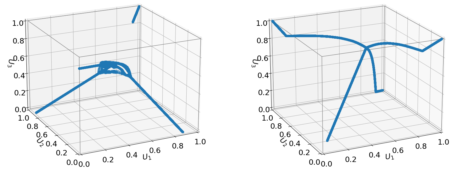
Figure 3: With $F_{i}\sim\log N(0,1)$ ($i=1,2,3$) and $n=100000$, the support of the copula that maximizes (resp. minimizes) coskewness is displayed in the left (resp. the right) panel. In this case, $M\approx 5.71$ and $m\approx-0.97$.

From Algorithm 3.1, we obtain that maximum and minimum coskewness are approximately equal to $5.71$ resp. $-0.97$ when $n=100000$. The supports of the corresponding copulas are displayed in Figure 3. Note that using the copulas coming from (3.3) resp. (3.5) would only lead to a coskewness equal to $4.79$ resp. $0.21$.

5 Conclusion

In this paper, we find new bounds for the expectation of a product of random variables when marginal distribution functions are fixed but dependence is unknown. We solve this problem explicitly under some conditions on the marginal distributions and propose an algorithm to solve the problem in the general case. We introduce the novel notion of standardized rank coskewness, which unlike coskewness, is unaffected by marginal distributions and thus appears useful for better understanding the degree of coskewness that exists among three random variables.

Acknowledgments:

The authors thank two reviewers for their valuable hints and remarks which helped to improve the paper. The authors gratefully acknowledge funding from Fonds Wetenschappelijk Onderzoek (grants FWOAL942 and FWOSB73). Jinghui Chen would like to thank Xin Liu for his comments on the paper.

References

- Bertino (1994) Bertino, S. (1994). The minimum of the expected value of the product of three random variables in the Fréchet class. Journal of the Italian Statistical Society 3(2), 201–211.
- Bignozzi and Puccetti (2015) Bignozzi, V. and G. Puccetti (2015). Studying mixability with supermodular aggregating functions. Statist. Probab. Lett. 100, 48–55.
- Gaffke and Rüschendorf (1981) Gaffke, N. and L. Rüschendorf (1981). On a class of extremal problems in statistics. Mathematische Operationsforschung und Statistik. Series Optimization 12(1), 123–135.
- Kotz et al. (2004) Kotz, S., N. Balakrishnan, and N. L. Johnson (2004). Continuous Multivariate Distributions, Volume 1: Models and Applications, Volume 1. John Wiley & Sons.
- Nelsen and Úbeda-Flores (2012) Nelsen, R. B. and M. Úbeda-Flores (2012). Directional dependence in multivariate distributions. Ann. Inst. Statist. Math. 64(3), 677–685.
- Puccetti et al. (2012) Puccetti, G., B. Wang, and R. Wang (2012). Advances in complete mixability. J. Appl. Probab. 49(2), 430–440.
- Puccetti and Wang (2015) Puccetti, G. and R. Wang (2015). Extremal dependence concepts. Statist. Sci. 30(4), 485–517.
- Rüschendorf (1980) Rüschendorf, L. (1980). Inequalities for the expectation of -monotone functions. Zeitschrift für Wahrscheinlichkeitstheorie und verwandte Gebiete 54(3), 341–349.
- Rüschendorf and Uckelmann (2002) Rüschendorf, L. and L. Uckelmann (2002). On the n-coupling problem. J. Multivariate Anal. 81(2), 242–258.
- Spearman (1904) Spearman, C. (1904). The proof and measurement of association between two things. The American Journal of Psychology 15(1), 72–101.
- Wang and Wang (2011) Wang, B. and R. Wang (2011). The complete mixability and convex minimization problems with monotone marginal densities. J. Multivariate Anal. 102(10), 1344–1360.
- Wang and Wang (2015) Wang, B. and R. Wang (2015). Extreme negative dependence and risk aggregation. J. Multivariate Anal. 136, 12–25.
- Wang and Wang (2016) Wang, B. and R. Wang (2016). Joint mixability. Math. Oper. Res. 41(3), 808–826.