Fooling the Image Dehazing Models by First Order Gradient

Abstract

The research on the single image dehazing task has been widely explored. However, as far as we know, no comprehensive study has been conducted on the robustness of the well-trained dehazing models. Therefore, there is no evidence that the dehazing networks can resist malicious attacks. In this paper, we focus on designing a group of attack methods based on first order gradient to verify the robustness of the existing dehazing algorithms. By analyzing the general purpose of image dehazing task, four attack methods are proposed, which are predicted dehazed image attack, hazy layer mask attack, haze-free image attack and haze-preserved attack. The corresponding experiments are conducted on six datasets with different scales. Further, the defense strategy based on adversarial training is adopted for reducing the negative effects caused by malicious attacks. In summary, this paper defines a new challenging problem for the image dehazing area, which can be called as adversarial attack on dehazing networks (AADN). Code and Supplementary Material are available at https://github.com/Xiaofeng-life/AADN_Dehazing.

I Introduction

The goal of image dehazing is to restore the clear scene from the hazy image [1, 2, 3, 4, 5], which is an important topic on low-level computer vision tasks. The image dehazing task [6] can be used as an upstream task of autonomous driving, traffic monitoring, and robot exploration, etc. Various dehazing networks have been proposed and verified on benchmark datasets [7, 8, 9, 10, 11, 12]. An important question is, do these dehazing models behave securely during the inference stage of practical applications? Unfortunately, the security of dehazing algorithms [3, 4, 5] has not received due attention. In this paper, we find that well-trained dehazing networks with high performance can be fooled by the attack methods based on first order gradient [13].

The existing dehazing networks [6] use different loss functions, network blocks and training strategies, but they may have two properties in common. First, the first-order gradient descent algorithm [6] is used for the training process. Second, one hazy image is taken as input and one dehazed image is provided as output without estimating the transmission map and atmospheric light in an explicit way during the inference stage. We call the dehazing methods that satisfy these two properties as the SISO (single input single output) dehazing networks. Within the scope of our study, we argue that SISO dehazing networks can be attacked by unified malicious attack algorithms.

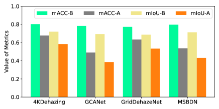
Figure 1: Attack results ($L_{P}^{MSE}$) on semantic segmentation dataset Foggy-City, where mACC and mIoU are two metrics for semantic segmentation. “-B” means before attack, and “-A” is after attack.

The results in Figure 10 show that after attacking the dehazing algorithm, the quality of the image is significantly reduced. Not only that, we found that the attack on the dehazing network will also cause the performance of the image segmentation algorithm, which may used as a downstream task of the dehazing task, to decline. Specifically, We choose the SegFormer [14] as the baseline segmentation network. The annotations for segmentation are from [15]. During the training stage, the segmentation network is trained on the original clear images in the dataset. During the inference stage, the inputs of the segmentation network are the outputs of the dehazing network. Figure 1 provides the quantitative evaluation of the segmentation task on the whole test dataset. It is an obvious conclusion that the attack on dehazing networks will lead to worse segmentation results.

Specifically, we propose two questions for the adversarial attack on dehazing networks (AADN) research as follows.

• Can the state-of-the-art dehazing models be attacked? What are the effective ways to attack them?

• If the dehazing models are vulnerable, how can we protect them in a proper way?

By obtaining the first-order gradient information, we successfully attack the dehazing models in a white-box manner. From the attacker’s perspective, unlike the class-based image classification task, the outputs of dehazing network are in pixel-wise form. The main difficulty is that the attacker may not have the “ground-truth label” for attacking. Therefore, we propose an attack method based on the predicted dehazed image that can avoid using the ground-truth label. Meanwhile, the difference in attack performance obtained using the ground-truth label versus the predicted dehazed image is studied. Then, considering that haze is not always uniformly distributed across the image, we design an attack method based on the haze-layer, which can partially attack haze images. Further, we explored how to preserve the haze in the hazy image, which means that the input and output of the dehazing network are almost identical. After finding that the dehazing networks can be attacked by the first order attack algorithm, a natural question is whether we can design a corresponding defense method to improve the performance after being attacked. Inspired by the research on robust image classification [13], an adversarial training strategy is adopted for the defense process. The main contributions of this paper are as follows.

• We define a new valuable research area called AADN. The study about adversarial attack and defense on dehazing task is conducted on various dehazing models and benchmark datasets.

• A pixel-wise white-box [16, 17] attack form is proposed for image dehazing task as the basic attack form, which is based on the first order gradient information during the backpropagation process.

• By analyzing the characteristics of SISO dehazing task, four attack methods are designed and verified on six benchmark datasets. The four attack methods are predicted dehazed image attack, hazy layer mask attack, haze-free image attack and haze-preserved attack, respectively.

• To explore if the attack effects can be reduced, the adversarial training is used for protecting the dehazing models with the target guiding way. Further, we find that adversarial defense training can improve the robustness of dehazing networks, but it can not “perfectly” protect the dehazing networks.

Our research shows that the SISO dehazing models can be attacked by the first-order gradient-based attack algorithm. Furthermore, we get three important conclusions. First, adversarial perturbations acquired with gradient information have significantly stronger negative effects on the dehazing model than regular noises. Second, the attacker only needs to use the outputs of dehazing models as pseudo-labels instead of using the ground-truth haze-free images as the guidance information for the attack process. Third, adversarial defense training can reduce the negative impacts caused by the attack algorithm, but it cannot completely eliminate these impacts. Meanwhile, adversarial defense training will slightly reduce the dehazing performance of the dehazing model on normal examples.

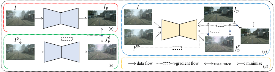
Figure 2: The pipelines of adversarial attack and defense on AADN. The contents of the four dotted boxes are (a) original dehazing process, (b) attack dehazing network, (c) adversarial defense training, and (d) illustration of arrows, respectively.

II Related Work

II-A Image Dehazing

Image dehazing algorithms aim at removing the haze on the hazy images [1, 2, 18, 19, 20]. The existing dehazing methods can be divided into DL-based and non-DL-based [6]. Overall, without considering the computation cost, the DL-based dehazing methods can achieve better performance than non-DL-based methods. However, our research shows the DL-based SISO dehazing models can be attacked by the first order attack algorithms.

Various dehazing networks [6] have been proposed by the researchers. DM2FNet [8] adopts four different feature functions and fuses them to the final output. The attention mechanism is applied in FFANet [10] and GridDehazeNet [11], which can obtain fine dehazing results. MSBDN [9] proves that boosting strategy and back projection can be used in the dehazing module, which can preserve spatial information by a symmetrical path. The contrastive learning is used for dehazing task by AECR-Net [21], which constructs the positive and negative pairs during the training process. DIDH [22] proposes to restore the high frequency and low frequency information by discriminator networks. RDN [23] proves that retinex model can be embedded to the dehazing process to obtain the residual illumination map and the dehazed image. PSD [24] takes a pre-trained and fine-tuning strategy to utilize the physical priors. DeHamer [25] uses the transformer architecture to implement the dehazing network. 4KDehazing [12] puts affine bilateral grid learning as a branch to the overall network that can process the high resolution image with high speed. Within the scope of SISO dehazing system, we find these well-known dehazing networks can be fooled by first order attack.

II-B Adversarial Attack and Defense

The adversarial attack and defense are important topics for artificial intelligence security [26, 27, 28, 29, 30, 31]. It is an interesting question to evaluate the robustness of neural networks under attack [32]. The research on adversarial attack argue that the well-trained networks may be fooled by hostile attack [33, 34]. By adding a small perturbation to the example, the prediction label generated by the classification network may change from “panda” (correct) to “gibbon” (incorrect) [33].

Goodfellow proposes a fast gradient sign method (FGSM)  [35] to generate the perturbation. FGSM is a one-step attack method which utilizes the gradient information calculated by the back propagation process. An iteration-based fast gradient sign method (i-FGSM) inspired by FGSM is explored by Kurakin et al. [36]. Instead of generating the perturbation by one step backward like FGSM, i-FGSM update the perturbation by multi-step and clip it into a fixed range. Besides, projected gradient descent (PGD) [13] is also a promising attack method to obtain the adversarial example that uses the multi-step update strategy. Inspired by PGD and  [37], the methods for attacking the dehazing networks are proposed in this paper.

Recent research has explored the topic on adversarial attack on image deraining [37], semantic segmentation [38, 39], super-resolution [40, 41, 42] and deblurring [43]. [40] proposes a method that leverages the generalization capability of adversarial attacks to tackle real-world super-resolution models. Extensive empirical evaluations in [41] show that image super-resolution can be an effective defense strategy against attack methods. Gao et al. [44] propose an adversarial haze synthetic process based on the atmospheric scattering model to fool the classifiers. Kanwal et al. [45] study how to use the haze to reduce or improve the performance of the person re-identification task. Sun et al. [46] propose a targeted adversarial attack to boost object detection performance after restoration. A new perspective is proposed by Sun’s research, which combines image dehazing with downstream tasks. The goal of  [44, 45, 46] are different from this paper, since our purpose is to attack the dehazing networks. To the best of our knowledge, no comprehensive research on the dehazing adversarial attack has been published yet.

This paper focuses on the white-box attack. White-box attack, gray-box attack and black-box attack are popular research areas currently [16, 17, 47]. White-box attack assumes the information of the networks can be obtained, like architecture and parameters. Gray-box attack and black-box attack assume the information is partially knowable and completely unknowable, respectively. In addition,  [48, 13] propose to treat the adversarial attack and defense as a game theoretic framework. In our experiments, we try to protect the dehazing network by adversarial training from the white-box attack.

III Methods

The important concepts for AADN are as follows, which are consistent with the whole paper.

• Attack: a process trying to reduce the performance of the well-trained dehazing networks by adding subtle perturbation to the hazy image.

• Attacker: a hostile attack algorithm, which can generate adversarial perturbation.

• Perturbation: a subtle signal generated by the attacker, and it is added to the hazy image.

• Adversarial example: a hazy image with perturbations.

• Defense: a process that tries to reduce the negative effects caused by the attacker.

The hazy image is denoted as $I$ and the corresponding ground-truth haze-free image is marked as $J$. $J_{p}$ stands for the predicted dehazed image obtained by dehazing network.

There are three important parts in this section. The basic attack form is introduced in Subsection III-A, which defines the general way to attack the SISO dehazing system. Subsection III-B describes four attack methods to disturb the dehazing networks. Subsection III-C shows the adversarial training defense strategy to obtain robust dehazing networks.

III-A Basic Attack Form

First-order based gradient optimization methods [6] are widely used for the SISO dehazing models. When attacking the dehazing model in a white-box manner, the gradient information is needed to calculate adversarial perturbations. Therefore, the first-order gradient information is adopted by our attack algorithm. The process of attacking the dehazing network is to add a perturbation $\delta$ to a hazy image $I$ and to obtain the adversarial example $I^{\delta}$, and this behavior makes the output ($J_{p}^{\delta}$) of dehazing network unpleasant, as follows,

$$J_{p}=\Gamma_{\theta}(I),$$ (1)

$$J_{p}^{\delta}=\Gamma_{\theta}(I+\delta)=\Gamma_{\theta}(I^{\delta}),$$ (2)

where $\Gamma_{\theta}$ denotes the pre-trained dehazing network with parameters $\theta$. The general optimization goal of image dehazing algorithms is to minimize one or more distance metrics, such as L1, L2, Perceptual [49] and structural similarity (SSIM) [50]. Therefore, the attacker tries to maximize these distance metrics, which will make the well-converged network have a higher loss value. The loss function $L_{att}$ that the attacker adopted is to maximize

$$L_{att}=\Re(J_{p}^{\delta},X),$$ (3)

where the $\Re(\cdot,\cdot)$ represents various loss functions for image restoration process and $X$ is the target that the attacker needs to use. Different $X$ can be adopted by the attacker so that the dehazed image after the attack tends to have different forms of quality degradation. During the attack process, the parameters $\theta$ of the network $\Gamma_{\theta}$ will not be updated. The attacker needs to learn the perturbation $\delta$, which is updated by the gradient values

$$\delta^{t+1}=\delta^{t}+\alpha sgn(\nabla_{\delta}L_{att}),$$ (4)

where $sgn$ is the sign function, $\alpha$ is the adjusting factor for updating process, $\nabla$ denotes gradient operation, and the $t$ denotes $t$-th iteration step. For each iteration, the input $I^{\delta}$ of $\Gamma_{\theta}$ is not static, which is changed by the perturbation. To ensure that the perturbation $\delta$ added to hazy image $I$ can not be easily observed, the value range of $\delta$ should be controlled. As proposed in [13], $\delta$ can be constrained by $\ell_{\infty}$. Further, $\delta$ will be clipped as

$$\delta^{t+1}=\kappa_{(-\epsilon,\epsilon)}(\delta^{t+1}),$$ (5)

where the $\kappa$ stands for clip operation and $\epsilon$ represents the range for clipping. $\epsilon=0$ denotes no attack. The pixel values of all images are normalized to $[0,1]$ during the training and inference stage. Therefore, the value range of attacked hazy image $I^{\delta}$ should also be limited to $[0,1]$, so $\delta$ is further clipped by

$$\delta^{t+1}=\kappa_{({0-I,1-I})}(\delta^{t+1}).$$ (6)

The above attack form can be used in both targeted and non-targeted ways. The aim of the targeted attack is forcing $J_{p}^{\delta}$ close to $X$. The goal of the non-targeted attack is trying to make $J_{p}^{\delta}$ far from $J$ visually.

III-B How to Attack

Subsection III-A gives the basic form about how to attack the dehazing networks. We propose that three important concepts that may be considered in the security of the dehazing task, namely the predicted dehazed image, the hazy image and the clear image. An attacker may use predicted dehazed images, hazy images and clear images to attack the dehazing models, respectively. When an attacker uses a predicted dehazed image or a clear image to attack the dehazing model, the output after the attack may deviate from the original output. When an attacker uses a hazy image to attack the dehazing model, the output after the attack may retain the haze in the image. Meanwhile, an attacker may perform partial attacks on the image. Considering the above factors, we designed four attack algorithms, which are predicted dehazed image attack $L_{P}$, hazy layer mask attack $L_{M}$, haze-free image attack $L_{G}$ and haze-preserved attack $L_{I}$, respectively.

III-B1 Predicted Dehazed Image Attack

Unlike image classification or semantic segmentation tasks, the ground-truth labels are not easy to be collected in the dehazing task. The hazy and haze-free pairs may not be annotated by humans. Therefore, we design an attack method based on predicted dehazed image $J_{p}$ that is obtained by the dehazing network $\Gamma_{\theta}$. The loss of the attack can be expressed by

$$L_{P}=\Re(\Gamma_{\theta}(I^{\delta}),J_{p}),$$ (7)

where $P$ in $L_{P}$ denotes prediction. The optimization goal is to maximize $L_{P}$ in a non-targeted way. Since such an attack method is non-targeted, a natural question is whether $L_{P}$ will cause the prediction result $\Gamma_{\theta}(I^{\delta})$ after the attack to be closer to the ground-truth image and whether it will lead to a failure attack. The experiments show that $L_{P}$ is a reliable and powerful attack method. The original dehazing process is shown in Figure 2 (a), and the process of attacking dehazing networks is displayed in Figure 2 (b).

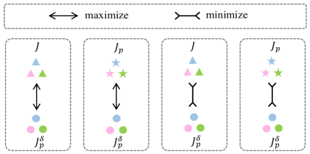
           (a) $L_{G}$             (b) $L_{P}$            (c) $L_{def}^{G}$          (d) $L_{def}^{P}$

Figure 3: The optimization direction of attack and defense.

III-B2 Haze Layer Mask Attack

Equation (7) provides an attack way based on the whole image. An interesting question is whether we can attack part of the hazy image and achieve impressive attack results. According to the atmospheric scattering model [51], the haze density of the pixels that are far from the camera is higher. This means that the haze is not always uniformly distributed across the image. Therefore, we propose the haze layer mask attack method which can partly attack the haze image, and the corresponding haze layer mask can be obtained by

$$\mu=\frac{1}{H\times W}\sum_{m=1}^{H}\sum_{n=1}^{W}(I(m,n)-J_{p}(m,n)),$$ (8)

$$mask=\left\{\begin{aligned} 1\quad(I(m,n)-J_{p}(m,n))>\mu,\\ 0\quad(I(m,n)-J_{p}(m,n))\leq\mu,\\ \end{aligned}\right.$$ (9)

where $H$ and $W$ denotes the height and width of the image, respectively. The loss function of haze layer mask attack is to maximize

$$L_{M}=\Re(\Gamma_{\theta}(I+\delta*mask),J_{p}),$$ (10)

where $*$ denotes pixel-wise multiplication and $M$ in $L_{M}$ stands for the mask.

III-B3 Haze-free Image Attack

Supposing the attacker already has the haze-free (ground-truth) image $J$, then the $J_{p}$ in attack loss $L_{P}$ can be replaced with $J$. The attack loss calculated by $J$ is

$$L_{G}=\Re(\Gamma_{\theta}(I^{\delta}),J),$$ (11)

where $G$ means ground-truth.

III-B4 Haze-preserved Attack

Considering an extreme situation that the output of the dehazing model totally contains the haze in the original hazy image. In this situation, the optimization object of the attacker is to minimize the distance between the dehazed image and the original hazy image by $\Re(\Gamma_{\theta}(I^{\delta}),I)$. We multiply $\Re(\Gamma_{\theta}(I^{\delta}),I)$ by “-1” so that minimizing $\Re(\Gamma_{\theta}(I^{\delta}),I)$ is equivalent to maximizing $-1*\Re(\Gamma_{\theta}(I^{\delta}),I)$, which is also equivalent to $-\Re(\Gamma_{\theta}(I^{\delta}),I)$. In this form, all attack loss functions proposed in this paper are optimized in a maximizing manner. The loss function for the haze-preserved attack is to maximize the following loss function

$$L_{I}=-1*\Re(\Gamma_{\theta}(I^{\delta}),I),$$ (12)

where the subscript in $L_{I}$ means identity output.

III-B5 The Distance Metrics

Here we choose two widely used distance metrics for $\Re(\cdot,\cdot)$, which are mean square error (MSE) and SSIM. The forms of MSE and SSIM are

$$MSE(x,y)=||x-y||_{2}^{2},$$ (13)

$$SSIM(x,y)=\frac{(2\mu_{x}\mu_{y}+C1)(2\delta_{xy}+C2)}{(\mu_{x}^{2}+\mu_{y}^{2}+C1)(\delta_{x}^{2}+\delta_{y}^{2}+C2)},$$ (14)

where $x$ and $y$ represent two images. C1 and C2 are constants. Details about SSIM can be found at [50]. The $\mu_{x}\&\mu_{y}$ and $\delta_{x}\&\delta_{y}$ denote mean and standard deviation, respectively. $\delta_{xy}$ is covariance. For convenience, the $L_{P}^{MSE}$ and $L_{P}^{SSIM}$ stand for the $L_{P}$ that using $MSE(x,y)$ and $1-SSIM(x,y)$ as the loss function, respectively.

Algorithm 1 The maximum number of iterations is set to $N$. The learning rate is denoted as $lr$. The iteration step of the attack process is $k$. $m$ is batch size. The boolean symbol $Tc$ is set to $True$ or $False$.

  Initialize the dehazing network $\Gamma_{\theta}$ by well-trained parameters.

  if $Tc$ then

     Initialize the Teacher network $\Gamma_{\theta}^{T}$.

  end if

  for the maximum number of iterations $N$ do

     Sample hazy images $I=\{i^{(1)},i^{(2)},\ldots,i^{(m)}\}$ and corresponding ground-truth images $J=\{j^{(1)},j^{(2)},\ldots,j^{(m)}\}$;

     if $Tc$ then

        Calculate the corresponding prediction $J_{p}^{T}=\{j_{p}^{T(1)},j_{p}^{T(2)},\ldots,j_{p}^{T(m)}\}$ by

        

$$J_{p}^{T}=\Gamma_{\theta}^{T}(I).$$ (15)

     end if

     Initialize $\delta$ by uniform distribution $U(-\epsilon,\epsilon)$ and $\delta$ is clipped by Equation 6;

     for $k$ steps do

        if $Tc$ then

           Calculate the attack loss $L_{P}$;

        else

           Calculate the attack loss $L_{G}$;

        end if

        Update $\delta$ by Equations 4, 5 and 6.

     end for

     Generate the attacked prediction $J_{p}^{\delta}$ by Equation 2;

     if $Tc$ then

        Calculate the adversarial training loss $L_{def}^{P}$;

     else

        Calculate the adversarial training loss $L_{def}^{G}$;

     end if

     Update parameters $\theta$ for $\Gamma_{\theta}$:

     

$$\theta=\theta-lr\times\nabla_{\theta}{L_{def}^{P}}.$$ (16)

  end for

III-C How to Defense

The attacker that adopts the white-box attack method can reduce the performance of the well-trained dehazing models. Therefore, we need to design the corresponding defense method to protect the vulnerable networks. There are two factors that we mainly consider.

• The defense method can be adopted by different dehazing models, rather than designed for a specific one.

• The inference time should not be increased by the defense method.

Based on the above two factors, we conduct the research on adversarial training defense [13] to protect the dehazing networks. However, the method in  [13] cannot be directly applied to the defense training of dehazing networks. The reason is that, as we analyzed when designing the attack algorithm, the target $X$ adopted by the attacker may not be a ground-truth image.

From the perspective of defense, the adversarial training process against the four attack methods can be divided into two categories. The first category is to use the original dehazed image $J_{p}$ to reduce the distance between the $J_{p}^{\delta}$ and $J_{p}$. Therefore, the adversarial training process may need to use the pre-trained dehazing model as a Teacher network to produce the original dehazed image $J_{p}$. This situation can be applied to $L_{P}$ and $L_{M}$. Figure 3 shows the optimization directions of attack and defense. From the attacker’s perspective, when using attack loss $L_{P}$, the distance between $J_{p}^{\delta}$ and $J_{p}$ is maximized as shown in Figure 3-(b). Therefore, theoretically, the defender should minimize the distance between $J_{p}^{\delta}$ and $J_{p}$ as shown in Figure 3-(d), since the gradient direction of Figure 3-(b) and Figure 3-(d) are complementary. However, the process shown in Figure 3-(d) requires the use of a fixed pre-trained model to calculate the $J_{p}$, which will increase the computational cost of the defense algorithm. Therefore, a possible way to eliminate the additional computational cost is to use the defense method shown in Figure 3-(c) (which is designed for Figure 3-(a)) to reduce the distance between $J_{p}^{\delta}$ and $J$. However, the gradient direction of Figure 3-(b) and Figure 3-(c) may not be complementary. Whether this way is feasible will be discussed and verified in the experimental section. The second category is to use clear image $J$ to reduce the distance between $J_{p}^{\delta}$ and $J$. This situation can be applied to $L_{J}$ and $L_{I}$.

Overall, two purposes are included in our research on defense training, as follows.

• When using Teacher network or ground-truth images for defense training, can we effectively resist the corresponding attack algorithm?

• Can the use of the Teacher network be avoided to reduce computing costs?

Based on the above purposes, two adversarial defense training processes are designed as shown in Algorithm 1. The attack methods are $L_{P}$ and $L_{G}$, respectively. In Algorithm 1, the boolean type variable $Tc$ is used to represent whether the Teacher network is utilized. When the value of $Tc$ is $True$, the calculated attack and defense losses are $L_{P}$ and $L_{def}^{P}$, respectively. On the contrary, when the value of $Tc$ is $False$, the calculated attack and defense losses are $L_{G}$ and $L_{def}^{G}$, respectively. Other attack methods can use Algorithm 1 for their own adversarial training processes. The adversarial training defense for $L_{P}$ and $L_{G}$ is a min-max (mm) game, as follows,

$$L_{mm}^{P}=\min_{\theta}\Re(J_{p}^{\delta},J_{p}^{T})\max_{||\delta||_{\infty}\leq\epsilon}\Re(J_{p}^{\delta},J_{p}^{T}),$$ (17)

$$L_{mm}^{G}=\min_{\theta}\Re(J_{p}^{\delta},J)\max_{||\delta||_{\infty}\leq\epsilon}\Re(J_{p}^{\delta},J).$$ (18)

Since the parameters $\theta$ of dehazing network $\Gamma_{\theta}$ will be changed during the adversarial training process, the Teacher network $\Gamma_{\theta}^{T}$ with fixed parameters is adopted to obtain predicted dehazed image $J_{p}^{T}$ ($J_{p}^{T}=\Gamma_{\theta}^{T}(I)$) for $L_{def}^{P}$. To ensure the dehazing network can still handle the hazy images $I$ that have not been attacked, the basic image restoration loss function should be adopted for the final defense loss. The overall losses of the corresponding defense methods for $L_{P}$ and $L_{G}$ are $L_{def}^{P}$ and $L_{def}^{G}$, which are defined as

$$L_{def}^{P}=\Re(\Gamma_{\theta}(I),J)+\lambda L_{mm}^{P},$$ (19)

$$L_{def}^{G}=\Re(\Gamma_{\theta}(I),J)+\lambda L_{mm}^{G},$$ (20)

where $\lambda$ is the balance factor for the original image restoration loss function and adversarial defense loss function. The adversarial training defense process does not need to start from scratch. The parameters can be initialized by the well-trained network, and fine-tuned on the adversarial examples. The overall pipeline about adversarial training defense $L_{def}^{P}$ is shown in Figure 2-(c).

TABLE I: Quantitative attack results obtained by $L_{P}^{MSE}$, $L_{M}^{MSE}$ and $L_{I}^{MSE}$. The “Method-$\epsilon$” denotes $\epsilon=i,i\in\{2,4,6,8\}$. The worst attack result and best attack result in each dehazing method are in blue and red, respectively. The dehazing results without attack are in bold.

Methods	ITS		OTS		4K		Foggy-City		I-HAZE		O-HAZE		D-Hazy
	PSNR$\uparrow$	SSIM$\uparrow$	PSNR$\uparrow$	SSIM$\uparrow$	PSNR$\uparrow$	SSIM$\uparrow$	PSNR$\uparrow$	SSIM$\uparrow$	PSNR$\uparrow$	SSIM$\uparrow$	PSNR$\uparrow$	SSIM$\uparrow$	PSNR$\uparrow$	SSIM$\uparrow$
4KDehazing	26.780	0.927	28.724	0.956	21.634	0.891	31.461	0.974	16.826	0.684	20.916	0.769	23.304	0.875
4KDehazing-P2	14.700	0.724	16.815	0.798	13.153	0.700	15.626	0.817	16.686	0.614	20.129	0.736	10.302	0.558
4KDehazing-P4	12.465	0.645	14.385	0.709	8.985	0.508	13.538	0.739	16.244	0.541	18.818	0.660	9.000	0.504
4KDehazing-P6	11.291	0.586	13.709	0.655	7.332	0.384	12.768	0.683	15.737	0.477	17.707	0.590	8.475	0.448
4KDehazing-P8	10.545	0.533	13.181	0.605	6.617	0.315	12.355	0.634	15.235	0.426	16.744	0.533	8.061	0.426
4KDehazing-M8	12.213	0.631	15.697	0.745	9.177	0.586	13.845	0.780	15.811	0.512	17.427	0.600	9.597	0.582
4KDehazing-I8	12.725	0.648	16.470	0.761	12.001	0.645	14.900	0.709	15.834	0.587	17.274	0.695	9.985	0.568
DM2FNet	29.922	0.954	29.323	0.957	26.651	0.943	32.582	0.971	17.368	0.711	23.519	0.754	28.252	0.937
DM2FNet-P2	13.782	0.681	17.343	0.802	11.769	0.687	15.978	0.821	15.372	0.661	16.059	0.604	8.385	0.404
DM2FNet-P4	11.912	0.610	15.160	0.709	9.288	0.564	14.694	0.762	13.999	0.595	12.435	0.508	7.100	0.296
DM2FNet-P6	11.423	0.593	14.596	0.657	8.856	0.511	14.275	0.708	13.916	0.561	11.454	0.475	6.823	0.274
DM2FNet-P8	11.214	0.570	14.464	0.617	8.624	0.476	14.010	0.650	13.265	0.495	10.899	0.454	6.813	0.268
DM2FNet-M8	11.983	0.652	15.766	0.736	10.397	0.644	14.874	0.792	14.338	0.608	12.485	0.539	8.746	0.540
DM2FNet-I8	12.207	0.644	16.285	0.748	12.367	0.634	14.852	0.754	14.681	0.558	15.541	0.640	9.729	0.582
FFANet	29.414	0.962	29.839	0.959	24.641	0.936	35.053	0.981	16.507	0.749	22.587	0.853	27.441	0.919
FFANet-P2	14.450	0.682	18.130	0.822	13.027	0.678	14.805	0.784	16.432	0.680	21.548	0.816	8.959	0.461
FFANet-P4	11.498	0.523	15.911	0.735	10.473	0.558	13.312	0.654	16.250	0.567	19.989	0.737	7.347	0.312
FFANet-P6	10.528	0.474	14.657	0.663	9.199	0.477	11.752	0.486	15.990	0.472	18.498	0.655	6.885	0.255
FFANet-P8	10.091	0.448	13.978	0.611	8.742	0.441	9.728	0.326	15.664	0.400	17.487	0.579	6.556	0.223
FFANet-M8	11.553	0.586	15.514	0.735	11.766	0.646	12.403	0.597	15.968	0.536	19.053	0.648	8.841	0.457
FFANet-I8	12.386	0.653	16.608	0.771	12.805	0.613	14.899	0.718	15.690	0.688	19.412	0.717	10.338	0.528
GCANet	25.880	0.895	27.808	0.943	23.266	0.880	31.541	0.968	16.535	0.669	20.599	0.717	24.209	0.881
GCANet-P2	11.879	0.537	14.744	0.719	13.274	0.682	14.901	0.787	16.565	0.632	18.211	0.680	9.665	0.557
GCANet-P4	8.981	0.359	10.760	0.527	9.798	0.537	12.006	0.652	14.571	0.547	16.686	0.609	8.203	0.458
GCANet-P6	7.925	0.301	9.336	0.448	8.574	0.459	10.931	0.568	14.106	0.484	14.967	0.512	7.395	0.392
GCANet-P8	7.530	0.283	8.733	0.407	7.990	0.409	10.433	0.516	13.353	0.424	14.200	0.455	6.932	0.354
GCANet-M8	9.485	0.453	10.803	0.598	10.050	0.554	12.971	0.742	14.409	0.540	15.389	0.519	8.410	0.502
GCANet-I8	13.433	0.645	17.739	0.755	12.010	0.599	15.656	0.726	15.843	0.585	17.659	0.600	10.492	0.563
GridDehazeNet	23.243	0.934	27.806	0.961	22.614	0.935	30.508	0.961	15.872	0.676	19.543	0.798	24.649	0.892
GridDehazeNet-P2	16.826	0.763	18.854	0.842	15.632	0.784	15.279	0.787	15.828	0.613	19.264	0.695	9.332	0.585
GridDehazeNet-P4	13.636	0.634	16.447	0.756	12.155	0.660	14.300	0.718	15.713	0.505	18.597	0.565	8.067	0.459
GridDehazeNet-P6	12.342	0.561	15.269	0.688	10.504	0.575	13.521	0.654	15.536	0.414	17.714	0.459	7.268	0.389
GridDehazeNet-P8	11.718	0.512	14.420	0.628	9.694	0.517	12.932	0.597	15.319	0.348	16.838	0.380	6.753	0.356
GridDehazeNet-M8	13.064	0.635	16.758	0.766	12.348	0.700	14.150	0.774	15.521	0.465	17.771	0.478	7.698	0.509
GridDehazeNet-I8	12.831	0.656	16.928	0.778	12.280	0.658	14.906	0.730	15.933	0.676	19.800	0.711	10.083	0.540
MSBDN	24.229	0.903	24.229	0.903	23.785	0.904	30.382	0.969	17.074	0.505	20.450	0.579	23.093	0.884
MSBDN-P2	13.845	0.691	13.845	0.691	13.769	0.737	15.824	0.788	16.209	0.448	18.596	0.540	9.510	0.561
MSBDN-P4	10.098	0.531	10.098	0.531	9.746	0.605	12.874	0.643	14.914	0.352	16.422	0.468	7.422	0.401
MSBDN-P6	8.243	0.430	8.243	0.430	8.543	0.538	11.814	0.555	13.936	0.273	14.866	0.396	6.594	0.333
MSBDN-P8	7.016	0.361	7.016	0.361	8.063	0.496	11.148	0.491	13.237	0.219	13.985	0.346	6.215	0.296
MSBDN-M8	8.948	0.488	15.347	0.703	9.550	0.602	13.025	0.739	14.597	0.338	15.086	0.400	7.610	0.476
MSBDN-I8	12.694	0.622	16.641	0.767	12.257	0.644	14.889	0.728	15.496	0.387	16.766	0.461	9.993	0.573

IV Experiments

The experiments contain three parts. Subsections IV-A and IV-B give the attack results and defense results, respectively. Subsection IV-C provides the ablation study and discussions. The P, M, I, G and S represent the $L_{P}^{MSE}$, $L_{M}^{MSE}$, $L_{I}^{MSE}$, $L_{G}^{MSE}$ and $L_{P}^{SSIM}$, respectively.

IV-A Experiments on Attack

TABLE II: Quantitative attack results obtained by $A_{N}$ and $L_{I}^{MSE}$. The worst attack result in each dehazing method is in blue.

Methods	ITS		OTS		4K		Foggy-City		I-HAZE		O-HAZE		D-Hazy
	PSNR$\uparrow$	SSIM$\uparrow$	PSNR$\uparrow$	SSIM$\uparrow$	PSNR$\uparrow$	SSIM$\uparrow$	PSNR$\uparrow$	SSIM$\uparrow$	PSNR$\uparrow$	SSIM$\uparrow$	PSNR$\uparrow$	SSIM$\uparrow$	PSNR$\uparrow$	SSIM$\uparrow$
4KDehazing-$A_{N}$	23.407	0.776	26.251	0.772	20.378	0.754	21.061	0.768	16.737	0.582	20.736	0.729	19.327	0.695
4KDehazing-I	12.725	0.648	16.470	0.761	12.001	0.645	14.900	0.709	15.834	0.587	17.274	0.695	9.985	0.568
DM2FNet-$A_{N}$	24.479	0.785	27.437	0.783	22.250	0.720	25.088	0.766	16.921	0.625	23.200	0.685	18.877	0.594
DM2FNet-I	12.207	0.644	16.285	0.748	12.367	0.634	14.852	0.754	14.681	0.558	15.541	0.640	9.729	0.582
FFANet-$A_{N}$	23.930	0.754	26.790	0.805	19.497	0.712	16.832	0.699	16.398	0.633	22.085	0.767	16.028	0.544
FFANet-I	12.386	0.653	16.608	0.771	12.805	0.613	14.899	0.718	15.690	0.688	19.412	0.717	10.338	0.528
GCANet-$A_{N}$	25.166	0.833	26.275	0.837	22.037	0.778	25.270	0.855	16.441	0.644	20.222	0.694	17.706	0.717
GCANet-I	13.433	0.645	17.739	0.755	12.010	0.599	15.656	0.726	15.843	0.585	17.659	0.600	10.492	0.563
GridDehazeNet-$A_{N}$	22.304	0.792	25.974	0.802	20.384	0.754	17.223	0.735	15.832	0.622	19.350	0.722	10.531	0.583
GridDehazeNet-I	12.831	0.656	16.928	0.778	12.280	0.658	14.906	0.730	15.933	0.676	19.800	0.711	10.083	0.540
MSBDN-$A_{N}$	23.367	0.787	27.145	0.811	22.837	0.792	26.072	0.776	16.906	0.414	20.110	0.513	21.366	0.694
MSBDN-I	12.694	0.622	16.641	0.767	12.257	0.644	14.889	0.728	15.496	0.387	16.766	0.461	9.993	0.573

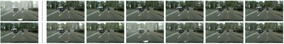
      (a) $I\&J$           (b) 4KDehazing     (c) DM2FNet      (d) FFANet       (e) GCANet   (f) GridDehazeNet   (g) MSBDN

Figure 4: Dehazing visual results obtained by $A_{N}$. The $\epsilon$ of top row and bottom row are 0 and 8, respectively. Images are from Foggy-City.

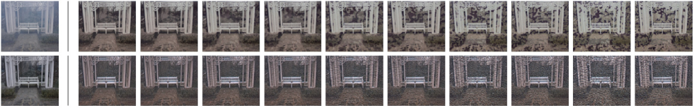
  (a) $I\&J$       (b) P-0      (c) M-0     (d) P-2     (e) M-2     (f) P-4     (g) M-4     (h) P-6      (i) M-6      (j) P-8     (k) M-8

Figure 5: Attack visual results obtained by $L_{P}^{MSE}$ and $L_{M}^{MSE}$. The $P-\epsilon$ and $M-\epsilon$ denote the results when $\epsilon\in\{0,2,4,6,8\}$. The algorithms of each row from up to down are 4KDehazing and GridDehazeNet, respectively. Images are from O-HAZE.

IV-A1 Settings on Attack

To show the attack results on different datasets with different scales, the experiments are conducted on six different datasets: ITS (indoor) and OTS (outdoor) from RESIDE [52], I-HAZE [53], O-HAZE [54], D-Hazy [55], 4K [12] and Foggy-City [56, 15]. The details about these datasets can be found in corresponding papers.

To ensure that the attack results are reliable, we choose the widely cited papers (dehazing algorithms) that are published on well-known conferences as baselines. The baselines methods are DM2FNet [8], GCANet [57], MSBDN [9], FFANet [10], GridDehazeNet [11] and 4KDehazing [12], respectively. The batch size is the same for all the baseline dehazing networks trained on the same dataset, that is $8$ for ITS/OTS/4K and $4$ for D-Hazy/I-HAZE/O-HAZE/Foggy-City. The image size for ITS/OTS/4K/I-HAZE/O-HAZE, D-Hazy and Foggy-City are $256\times 256$, $480\times 640$ and $256\times 512$, respectively. We choose the widely used metric PSNR and SSIM [50] for the evaluation, which are consistent with our attack loss functions. Lower PSNR and SSIM value stand for worse dehazing result, while representing better attack performance. When evaluating the performance of the model before and after the attack, we used exactly the same experimental settings. The dimensionalities of the input hazy image and the parameters of the dehazing model are exactly the same. Therefore, the reason for the degradation in model performance is the adversarial perturbations generated by our proposed attack algorithm.

The choice of parameters is theoretically infinite. For the attack experiments, the $\epsilon$ is chosen from $\{0,2,4,6,8\}$, and $\alpha$ is set to $2$. Both $\epsilon$ and $\alpha$ are divided by 255. The $\epsilon=0$ means no attack. The attack iteration steps are $10$. Initialized values of $\delta$ for attacking and the noise for noise attack $A_{N}$ are both sampled from uniform distribution $U(-\epsilon,\epsilon)$. The attack methods contain $L_{P}^{MSE}$, $A_{N}$, $L_{M}^{MSE}$, $L_{G}^{MSE}$, $L_{I}^{MSE}$ and $L_{P}^{SSIM}$, respectively. The attack process is to maximize these loss functions (except noise attack $A_{N}$). It is worth noting that the $mask$ in $L_{M}$ ($L_{M}^{MSE}$) has three channels obtained by copying a single channel. The $\mu$ used to obtain the $mask$ is calculated on the whole image (channel average) as shown in Equation 9. Any position $(m,n)$ in the hazy image $I$ is either be attacked or not attacked. Therefore, $mask(m,n)$ equals $1$ when any channel in position $(m,n)$ satisfied $I(m,n)-J_{p}(m,n)>\mu$.

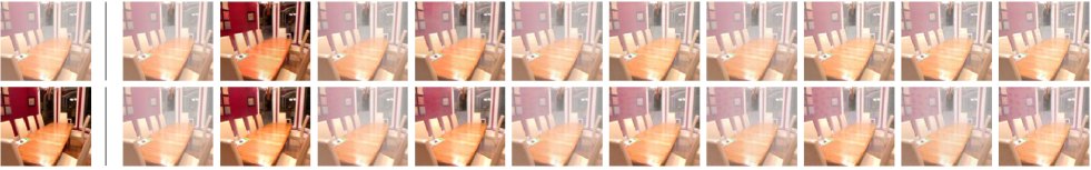
  (a) $I\&J$        (b) $I^{\delta}$-0    (c)$J_{p}^{\delta}$-0     (d) $I^{\delta}$-2    (e) $J_{p}^{\delta}$-2    (f) $I^{\delta}$-4     (g) $J_{p}^{\delta}$-4    (h) $I^{\delta}$-6     (i) $J_{p}^{\delta}$-6     (j) $I^{\delta}$-8     (k) $J_{p}^{\delta}$-8

Figure 6: Attack visual results obtained by $L_{I}^{MSE}$. The attacked hazy image and corresponding prediction (dehazed image) are denoted as $I^{\delta}-\epsilon$ and $J_{p}^{\delta}-\epsilon$, respectively. $\epsilon\in{\{0,2,4,6,8\}}$. The algorithms of each row from up to down are 4KDehazing and GridDehazeNet, respectively. Images are from ITS.

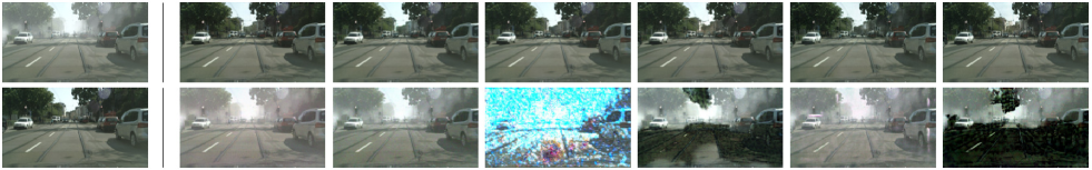
      (a) $I\&J$          (b) 4KDehazing    (c) DM2FNet       (d) FFANet      (e) GCANet    (f) GridDehazeNet   (g) MSBDN

Figure 7: Attack visual results obtained by attack loss $L_{G}^{MSE}$. The $\epsilon$ of each row from up to down are 0 and 8, respectively. Images are from Foggy-City.

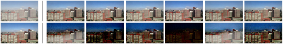
      (a) $I\&J$          (b) 4KDehazing    (c) DM2FNet       (d) FFANet      (e) GCANet    (f) GridDehazeNet   (g) MSBDN

Figure 8: Image dehazing visual results obtained by different dehazing algorithms under attack loss $L_{P}^{SSIM}$. The $\epsilon$ of each row from up to down are 0 and 8, respectively. Images are from OTS.

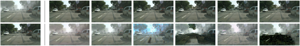
      (a) $I\&J$          (b) 4KDehazing    (c) DM2FNet       (d) FFANet      (e) GCANet    (f) GridDehazeNet   (g) MSBDN

Figure 9: Image dehazing visual results obtained by different dehazing algorithms under attack loss $L_{P}^{MSE}$. The $\epsilon$ of each row from up to down are 0 and 8, respectively. Images are from Foggy-City.

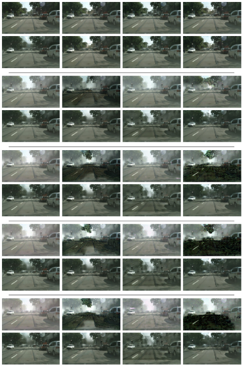
  (a) 4KDehazing       (b) GCANet      (c) GridDehazeNet     (d) MSBDN

Figure 10: Image dehazing results obtained by different dehazing algorithms under attack loss $L_{P}^{MSE}$ before and after defense training. Every two rows of images are in a group. The above images of each group are the results of direct attack (without defense training), and the bottom images are the results of attack after defense training. The $\epsilon$ of two rows from up to down are 0, 2, 4, 6 and 8, respectively. Images are from Foggy-City.

IV-A2 Results on Attack

Here, quantitative and visual evaluations of the attack results are given. Furthermore, the corresponding conclusions and analyses are provided.

• Attack by $L_{P}^{MSE}$: Table I shows the dehazing performance obtained by different dehazing methods on various benchmark datasets without being attacked. When there is no attack, these dehazing models are able to achieve impressive performance. However, when they were attacked by our proposed $L_{P}^{MSE}$, the values of PSNR and SSIM dropped significantly. As $\epsilon$ increases from 2 to 8, the attack performance gradually increases. The visual results obtained by the dehazing networks after attacks on the Foggy-City dataset are shown in Figure 9. It can be seen that the visual dehazing results after the attack are quite unsatisfactory. The quantitative and visual results demonstrate that the attacker can use predicted dehazed images obtained by dehazing networks as pseudo labels to attack the dehazing networks.

• Attack by $L_{M}^{MSE}$: Table I shows the attack results obtained by $L_{M}^{MSE}$. Overall, the attack results obtained by $L_{M}^{MSE}$ are slightly lower than those of $L_{P}^{MSE}$. This result is intuitive since $L_{M}^{MSE}$ only performed the attack on areas with high haze density, rather than the entire hazy image. Figure 5 compares the visual performance between the haze layer mask attack and the non-mask attack method. The haze layer mask attack can achieve similar effects as the non-mask attack, which shows that the attacker can partially attack the input hazy image, rather than the whole image.

• Attack by $L_{I}^{MSE}$: As shown in Table I, the attack results obtained by $L_{MSE}$ are lower than those of $L_{P}^{MSE}$ and $L_{M}^{MSE}$. The possible reason for this phenomenon is that the purpose of $L_{I}$ is to preserve the haze in the image, which does not destroy the content and structure of the image. The attacked hazy images $I^{\delta}=I+\delta$ and predicted attacked dehazed images $J_{p}^{\delta}$ shown in Figure 6 are quite close from the perspective of visual perception when $\epsilon>0$. This phenomenon illustrates that the haze-preserved attack loss $L_{I}^{MSE}$ can preserve the haze inside the hazy images.

• Attack by $L_{P}^{SSIM}$: Table IV compares the values of quantitative results obtained by $L_{P}^{SSIM}$ and $L_{P}^{MSE}$. The $\epsilon$ is set to $8$. $L_{P}^{SSIM}$ is a direct attack on SSIM metrics. $L_{P}^{MSE}$ is an approximately direct attack on PSNR since PSNR is inversely proportional to MSE. The results show that the value of PSNR decreases more when using $L_{P}^{MSE}$, while the value of SSIM decreases more when using $L_{P}^{SSIM}$. Quantitative attack results show that the first-order gradient can effectively attack both PSNR and SSIM metrics. Figure 8 shows the outdoor attack results obtained by attack loss $L_{P}^{SSIM}$. Under the attack of $L_{P}^{SSIM}$, the visual quality of dehazed images all decreases, which shows the effectiveness of the attack method based on SSIM loss.

According to the experimental results obtained by attack methods $L_{P}^{MSE}$, $L_{M}^{MSE}$, $L_{I}^{MSE}$ and $L_{P}^{SSIM}$, three valuable conclusions can be drawn. First, the attacker can use first-order gradient information to successfully attack the dehazing model. Second, using dehazed images as attack targets achieves better attack results than using hazy images. Third, taking $MSE$ and $SSIM$ as the loss function in the attack process can improve the attack performance of PSNR and SSIM, respectively.

TABLE III: Quantitative attack results obtained by $L_{P}^{MSE}$ and $L_{G}^{MSE}$. The best attack result in each dehazing method is in red.

Methods	ITS		OTS		4K		Foggy-City		I-HAZE		O-HAZE		D-Hazy
	PSNR$\uparrow$	SSIM$\uparrow$	PSNR$\uparrow$	SSIM$\uparrow$	PSNR$\uparrow$	SSIM$\uparrow$	PSNR$\uparrow$	SSIM$\uparrow$	PSNR$\uparrow$	SSIM$\uparrow$	PSNR$\uparrow$	SSIM$\uparrow$	PSNR$\uparrow$	SSIM$\uparrow$
4KDehazing-P	10.545	0.533	13.181	0.605	6.617	0.315	12.355	0.634	15.235	0.426	16.744	0.533	8.061	0.426
4KDehazing-G	10.131	0.505	11.845	0.532	7.031	0.359	12.250	0.625	13.335	0.394	14.950	0.537	6.713	0.278
DM2FNet-P	11.214	0.570	14.464	0.617	8.624	0.476	14.010	0.650	13.265	0.495	10.899	0.454	6.813	0.268
DM2FNet-G	11.073	0.556	10.479	0.371	7.933	0.427	13.763	0.642	11.893	0.442	10.785	0.421	6.537	0.235
FFANet-P	10.091	0.448	13.978	0.611	8.742	0.441	9.728	0.326	15.664	0.400	17.487	0.579	6.556	0.223
FFANet-G	10.063	0.437	12.279	0.537	8.726	0.448	9.760	0.326	14.010	0.499	15.938	0.601	6.552	0.227
GCANet-P	7.530	0.283	8.733	0.407	7.990	0.409	10.433	0.516	13.353	0.424	14.200	0.455	6.932	0.354
GCANet-G	7.111	0.299	7.557	0.272	7.789	0.421	10.538	0.522	11.907	0.422	13.990	0.465	6.822	0.346
GridDehazeNet-P	11.718	0.512	14.420	0.628	9.694	0.517	12.932	0.597	15.319	0.348	16.838	0.380	6.753	0.356
GridDehazeNet-G	11.956	0.581	12.156	0.547	9.416	0.491	12.700	0.586	14.011	0.434	14.950	0.429	6.714	0.354
MSBDN-P	7.016	0.361	7.016	0.361	8.063	0.496	11.148	0.491	13.237	0.219	13.985	0.346	6.215	0.296
MSBDN-G	6.875	0.388	11.523	0.522	7.829	0.457	10.713	0.442	12.105	0.165	12.420	0.298	5.738	0.226

TABLE IV: Quantitative attack results obtained by $L_{P}^{MSE}$ and $L_{P}^{SSIM}$. The best attack result in each dehazing method is in red.

Methods	ITS		OTS		4K		Foggy-City		I-HAZE		O-HAZE		D-Hazy
	PSNR$\uparrow$	SSIM$\uparrow$	PSNR$\uparrow$	SSIM$\uparrow$	PSNR$\uparrow$	SSIM$\uparrow$	PSNR$\uparrow$	SSIM$\uparrow$	PSNR$\uparrow$	SSIM$\uparrow$	PSNR$\uparrow$	SSIM$\uparrow$	PSNR$\uparrow$	SSIM$\uparrow$
4KDehazing-P	10.545	0.533	13.181	0.605	6.617	0.315	12.355	0.634	15.235	0.426	16.744	0.533	8.061	0.426
4KDehazing-S	12.381	0.357	13.436	0.424	10.547	0.193	13.273	0.433	15.589	0.254	17.733	0.259	9.135	0.101
DM2FNet-P	11.214	0.570	14.464	0.617	8.624	0.476	14.010	0.650	13.265	0.495	10.899	0.454	6.813	0.268
DM2FNet-S	11.411	0.397	12.691	0.409	9.542	0.328	14.699	0.433	15.561	0.388	14.851	0.509	8.142	0.081
FFANet-P	10.091	0.448	13.978	0.611	8.742	0.441	9.728	0.326	15.664	0.400	17.487	0.579	6.556	0.223
FFANet-S	11.072	0.245	14.456	0.438	11.359	0.273	8.702	0.187	15.554	0.283	19.492	0.343	9.615	0.022
GCANet-P	7.530	0.283	8.733	0.407	7.990	0.409	10.433	0.516	13.353	0.424	14.200	0.455	6.932	0.354
GCANet-S	7.904	0.198	10.084	0.334	10.742	0.153	12.866	0.342	14.834	0.219	16.660	0.208	8.989	0.185
GridDehazeNet-P	11.718	0.512	14.420	0.628	9.694	0.517	12.932	0.597	15.319	0.348	16.838	0.380	6.753	0.356
GridDehazeNet-S	13.083	0.395	13.476	0.435	13.179	0.341	14.618	0.420	15.189	0.264	17.243	0.173	9.337	0.158
MSBDN-P	7.016	0.361	7.016	0.361	8.063	0.496	11.148	0.491	13.237	0.219	13.985	0.346	6.215	0.296
MSBDN-S	8.453	0.316	12.928	0.435	12.671	0.309	14.201	0.248	14.945	0.182	17.269	0.222	7.595	0.129

IV-B Experiments on Defense

IV-B1 Settings on Defense

The $\lambda$ in Equations (19) and (20) are set to 1. The epochs for defense training are set to 40 and $\epsilon$ is fixed as $8$ (maximum attack degree). Since the adversarial examples are generated dynamically, the adversarial defense training time under each epoch is almost $k$ (iteration steps for generating $\delta$) times of the original training time. The defense training strategy is verified by using 4KDehazing, GCANet, GridDehazeNet and MSBDN.

IV-B2 Results on Defense

Here we show the attack results after adversarial defense training both quantitatively and visually. In addition, the summaries and analyses of the defense results are also provided. The “Method-$\epsilon$” denote the attack results when $\epsilon=i,i\in\{2,4,6,8\}$. TP denotes trained by $L_{def}^{P}$, and TG means trained by $L_{def}^{G}$. Table VII shows the quantitative attack results before and after defense training. The results summarized from Table VII are as follows.

• The adversarial defense training is quite effective for protecting the dehazing networks and the dehazing performance after defense training is obviously better (higher PSNR and SSIM) than that before defense training. Meanwhile, with the increases of $\epsilon$, the PSNR and SSIM that after defense training decrease more slowly than that before defense training.

• “TP” and “TG” in Table VII show the dehazing results on original hazy examples $I$ (without attack). It can be seen that adversarial defense training will slightly reduce the dehazing performance on original hazy examples in most cases.

Figure 10 shows the visual attack results before and after defense training. It can be seen that the attack results after defense training are more visually pleasing than those before defense training. The quality of image texture and detail is improved by defense training.

The main conclusion summarized from the quantitative and visual results is that the adversarial defense training can protect the dehazing networks, but it can not “totally” eliminate the negative effects caused by the attacker. The reason is that the dehazing model has seen the adversarial examples during defense training, so its robustness is improved. However, the attacker is still able to obtain the gradient information of the dehazing model that has performed the defense training [16]. Therefore, the attacker can still suboptimally find the weaknesses of the dehazing model. The distribution of original hazy images is denoted as $P_{I}$, the distribution of original hazy images and hazy images that after adding adversarial perturbations is denoted as $P_{I+I^{\delta}}$, and distribution of clear images $J$ is $P_{J}$. The regular training process is to learn the mapping from $P_{I}$ to $P_{J}$, while the defense training process learns the mapping from $P_{I+I^{\delta}}$ to $P_{J}$. The goals of defense training and regular training are different. This phenomenon is consistent with the classification task [13], which leads to the need for a balance between the robustness and the performance of the model [58]. Therefore, the performance of the dehazing model that after defense training on the original hazy image will be slightly worse.

IV-B3 Analysis of the Teacher Network

Table V shows the results obtained using $L_{P}^{MSE}$ for attack after defense training using $L_{def}^{P}$ and $L_{def}^{G}$, respectively. The results in Table V are on the Foggy-City dataset. The results show that the defense results obtained by using $L_{def}^{G}$ and $L_{def}^{P}$ against $L_{P}^{MSE}$ are comparable. The results demonstrate that the additional computational cost of using a Teacher network can be avoided.

IV-B4 Multi-step Attack and Defense

The attacker takes an iteration-based strategy to attack the dehazing networks. The iteration step is $k$. To investigate how $k$ affects the attack and defense performance, we set $k$ to different values and calculate the corresponding dehazing results. The $\epsilon$ is set to $4$. Table VI shows the attack results obtained by attack loss $L_{P}^{MSE}$ when $k\in\{1,2,3,5,10,15,20,25,30\}$. The results in Table VI indicate that with the increases of $k$, the attack performance increases in most cases. The attack effect does not increase significantly when $k>10$. The possible reason for this phenomenon is that the value of $\epsilon$ is limited to $4$. Therefore, the attack effect of an attacker who modifies the pixel value within the range $(-4,4)$ will not continue to grow rapidly.

For adversarial defense training stage, $k$ is randomly selected from $\{20,25,30\}$ in each iteration. The attack results before and after defense training are shown in Table VI, which can achieve the same conclusions as the situation where the step size of defense training is fixed. The results indicate that adversarial defense training with the multi-step attack is effective when the attacker adopts different attack iterations ($k$) in most cases.

TABLE V: Attack result obtained by $L_{P}^{MSE}$ after training by $L_{def}^{G}$ and $L_{def}^{P}$, respectively. PSNR and SSIM are displayed in the form of A/B, where A denotes the defense loss $L_{def}^{G}$ and B means the defense loss $L_{def}^{P}$.

Methods	4KDehazing		GCANet		GridDehazeNet		MSBDN
	PSNR$\uparrow$	SSIM$\uparrow$	PSNR$\uparrow$	SSIM$\uparrow$	PSNR$\uparrow$	SSIM$\uparrow$	PSNR$\uparrow$	SSIM$\uparrow$
$\epsilon=2$	24.258/24.413	0.905/0.906	23.619/23.486	0.899/0.895	20.763/21.059	0.858/0.850	23.545/23.380	0.891/0.887
$\epsilon=4$	23.604/23.918	0.885/0.884	22.701/22.581	0.875/0.872	20.175/20.406	0.832/0.819	22.316/22.211	0.868/0.865
$\epsilon=6$	22.843/23.193	0.853/0.850	21.814/21.701	0.844/0.842	19.631/19.825	0.797/0.782	21.299/21.218	0.842/0.839
$\epsilon=8$	22.108/22.501	0.807/0.803	20.999/20.879	0.804/0.805	19.087/19.207	0.754/0.740	20.487/20.427	0.813/0.811

TABLE VI: Quantitative defense results obtained by $L_{def}^{P}$ on D-Hazy. PSNR and SSIM are displayed in the form of A/B, where A is the result after defense training and B is the result before defense training, respectively. The bold value in A/B represents a better defense result.

Methods	4KDehazing		GCANet		GridDehazeNet		MSBDN
	PSNR$\uparrow$	SSIM$\uparrow$	PSNR$\uparrow$	SSIM$\uparrow$	PSNR$\uparrow$	SSIM$\uparrow$	PSNR$\uparrow$	SSIM$\uparrow$
no attack	15.172/23.304	0.747/0.875	22.829/24.209	0.838/0.881	24.840/24.649	0.890/0.892	17.109/23.093	0.779/0.884
$k=1$	15.142/14.534	0.693/0.668	15.752/12.088	0.733/0.649	15.687/9.969	0.735/0.599	16.921/13.056	0.708/0.639
$k=2$	15.131/11.143	0.669/0.596	15.457/9.996	0.725/0.547	15.533/9.346	0.729/0.570	16.749/9.703	0.683/0.532
$k=3$	15.131/10.057	0.658/0.560	15.247/9.307	0.718/0.510	15.453/9.063	0.724/0.548	16.702/8.667	0.681/0.493
$k=5$	15.135/9.536	0.653/0.534	15.057/8.701	0.710/0.477	15.400/8.647	0.721/0.514	16.535/7.997	0.693/0.443
$k=10$	15.156/8.918	0.658/0.493	15.009/8.148	0.708/0.451	15.372/8.080	0.720/0.459	16.289/7.492	0.714/0.421
$k=15$	15.164/8.839	0.662/0.482	15.001/7.988	0.708/0.442	15.370/7.830	0.720/0.434	16.371/7.413	0.719/0.408
$k=20$	15.170/8.462	0.665/0.474	15.000/7.837	0.708/0.437	15.365/7.649	0.720/0.417	16.340/7.305	0.724/0.399
$k=25$	15.174/8.464	0.667/0.460	15.003/7.750	0.708/0.432	15.365/7.538	0.720/0.407	16.314/7.239	0.725/0.389
$k=30$	15.174/8.397	0.668/0.467	15.000/7.725	0.708/0.431	15.363/7.446	0.720/0.398	16.262/7.285	0.727/0.396

TABLE VII: Quantitative defense results obtained by $L_{def}^{P}$ and $L_{def}^{G}$ on test datasets. PSNR and SSIM are displayed in the form of A/B, where A is the result after defense training and B is the result before defense training. The bold value in A/B (when $\epsilon>0$) represents a better defense result.

Methods	TP				TG
	D-Hazy		Foggy-City		D-Hazy		Foggy-City
	PSNR$\uparrow$	SSIM$\uparrow$	PSNR$\uparrow$	SSIM$\uparrow$	PSNR$\uparrow$	SSIM$\uparrow$	PSNR$\uparrow$	SSIM$\uparrow$
4KDehazing-0	15.250/23.304	0.745/0.875	24.533/31.461	0.912/0.974	15.532/23.304	0.753/0.875	24.458/31.461	0.909/0.974
4KDehazing-2	15.313/10.302	0.739/0.558	24.413/15.626	0.906/0.817	15.142/9.363	0.732/0.437	23.390/15.273	0.893/0.792
4KDehazing-4	15.317/9.000	0.705/0.504	23.918/13.538	0.884/0.739	14.753/7.574	0.704/0.324	22.227/13.142	0.868/0.711
4KDehazing-6	15.248/8.475	0.648/0.448	23.193/12.768	0.850/0.683	14.374/6.983	0.672/0.293	21.168/12.567	0.837/0.667
4KDehazing-8	15.115/8.061	0.576/0.426	22.501/12.355	0.803/0.634	14.005/6.713	0.636/0.278	20.256/12.250	0.800/0.625
GCANet-0	22.974/24.209	0.843/0.881	30.063/31.541	0.957/0.968	22.655/24.209	0.836/0.881	30.335/31.541	0.958/0.968
GCANet-2	15.463/9.665	0.736/0.557	23.486/14.901	0.895/0.787	15.358/9.505	0.727/0.545	23.461/14.921	0.894/0.785
GCANet-4	15.074/8.20	0.712/0.458	22.581/12.006	0.872/0.652	14.922/8.052	0.701/0.443	22.480/12.107	0.871/0.653
GCANet-6	14.645/7.395	0.683/0.392	21.701/10.931	0.842/0.568	14.475/7.283	0.671/0.381	21.562/11.050	0.841/0.573
GCANet-8	14.253/6.932	0.650/0.354	20.879/10.433	0.805/0.516	14.070/6.822	0.639/0.346	20.722/10.538	0.806/0.522
GridDehazeNet-0	24.261/24.649	0.869/0.892	29.970/30.508	0.957/0.961	24.834/24.649	0.885/0.892	29.753/30.508	0.956/0.961
GridDehazeNet-2	14.795/9.332	0.722/0.585	21.059/15.279	0.850/0.787	15.626/9.316	0.732/0.585	20.773/15.082	0.855/0.781
GridDehazeNet-4	14.705/8.067	0.708/0.459	20.406/14.300	0.819/0.718	15.402/8.028	0.713/0.457	20.144/13.924	0.829/0.704
GridDehazeNet-6	15.085/7.268	0.690/0.389	19.825/13.521	0.782/0.654	15.114/7.226	0.687/0.388	19.579/13.220	0.795/0.641
GridDehazeNet-8	14.824/6.753	0.656/0.356	19.207/12.932	0.740/0.597	14.690/6.714	0.653/0.354	19.011/12.700	0.753/0.586
MSBDN-0	22.771/23.093	0.865/0.884	29.370/30.382	0.964/0.969	22.399/23.093	0.864/0.884	29.671/30.382	0.964/0.969
MSBDN-2	16.068/9.510	0.746/0.561	23.380/15.824	0.887/0.788	15.723/8.827	0.739/0.485	23.421/15.411	0.888/0.770
MSBDN-4	15.428/7.422	0.715/0.401	22.211/12.874	0.865/0.643	15.063/6.858	0.704/0.330	22.139/12.277	0.866/0.586
MSBDN-6	14.836/6.594	0.676/0.333	21.218/11.814	0.839/0.555	14.469/6.156	0.665/0.261	21.101/11.216	0.839/0.492
MSBDN-8	14.311/6.215	0.634/0.296	20.427/11.148	0.811/0.491	13.950/5.738	0.624/0.226	20.269/10.713	0.812/0.442

IV-C Ablation Study and Discussions

IV-C1 Noise Attack and Gradient-based Attack

The perturbation generated by the attacker can be seen as a specific noise information that is added to the hazy image. Therefore, we need to compare the attack results between the perturbation and the general noise to verify the effectiveness of the adversarial attack. The noise attack is marked as $A_{N}$, where $N$ denotes the noise sampling from noise distribution. It is worth noting that $A_{N}$ directly generates the $\delta$ by noise distribution, rather than using the gradient descent algorithm. The $A_{N}$ is mainly used to prove that the learned perturbation has stronger attack effects than general noise. Since the perturbation is initialized with a uniform distribution, the noise is also sampled from a uniform distribution. As our experimental results show, $L_{I}^{MSE}$ is the attack loss function with the overall worst attack performance in the quantitative evaluation. We compare noise attack $A_{N}$ and haze-preserved attack $L_{I}^{MSE}$ under the same experimental setting. The noise level of $A_{N}$ is set to $[-8,8]$, which is consistent with the $\epsilon$ of $L_{I}^{MSE}$.

Table II shows the attack performance of $A_{N}$ and $L_{I}^{MSE}$ against different dehazing methods. The results on all datasets demonstrate that the performance of noise attack is significantly lower than that of $L_{I}^{MSE}$. The visual results in Figure 4 show the original dehazed outputs ($\epsilon=0$) and the predicted attacked outputs ($\epsilon=8$). Although $\epsilon$ is set to 8, the texture and structure of attacked outputs are still consistent with the original dehazed outputs. It can be concluded that all the attack algorithms proposed in this paper are significantly better than noise in attacking dehazing networks in terms of both quantitative and visual evaluation. The reason is that the $\delta$ is generated by adjusting the distance between $J_{p}^{\delta}$ and $X$. Moreover, the generation process of the $\delta$ utilizes the specific dehazing model. However, these two factors are not available in regular noise. Therefore, the attack effect of $\delta$ is stronger than regular noise.

IV-C2 Attack without Ground-truth

Table III shows the attack results of $L_{G}^{MSE}$, in which the ground truth haze-free label is used in the attack process. The $\epsilon$ is set to $8$. Quantitative evaluation results show that the overall attack performance of $L_{G}^{MSE}$ is slightly better than that of $L_{P}^{MSE}$. It is reasonable that the attack effect of $L_{G}^{MSE}$ is slightly better than that of $L_{P}^{MSE}$ since the reference used in the calculation of quantitative metrics is the ground-truth haze-free image. The visual dehazed results $J_{p}^{\delta}$ obtained by attack loss $L_{G}^{MSE}$ are shown in Figure 7. The attack visual performances of Figure 7 are quite close to the attack visual performance obtained by attack loss $L_{P}^{MSE}$ that is shown in Figure 9. The quantitative and visual results demonstrate that taking predicted dehazed images ($J_{p}$) as pseudo labels is a promising way to attack the dehazing networks.

IV-C3 Segmentation Results after Defense Training

Figure 1 shows the segmentation results under attack $L_{P}^{MSE}$ when $\epsilon$ is set to $4$. Figure 11 gives the quantitative segmentation results after adversarial defense training and shows two interesting phenomenons. First, the segmentation results when there is no attack ($\epsilon=0$) in Figure 11 are lower than that in Figure 1. This is consistent with the dehazing results ($\epsilon=0$) before and after defense training. Comparing Figure 1 with Figure 11, we can find that the robustness of segmentation has been improved to a certain extent after defense training.

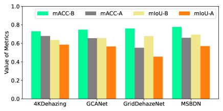
Figure 11: Attack results ($L_{P}^{MSE}$) on semantic segmentation dataset Foggy-City after defense training, where mACC and mIoU are two metrics for semantic segmentation. “-B” means before attack, and “-A” is after attack.

V Conclusion

In this paper, we try to explore and define a new research problem, which is called AADN. A first order attack algorithm is found to be powerful to attack the dehazing networks, which will lead to the performance reduction of the dehazing task. Meanwhile, several attack forms are proposed and verified for different attack purposes. Finally, we explore the effectiveness of adversarial defense training to protect vulnerable dehazing networks. We have investigated the fundamental problems of attacking dehazing networks. Since we must control the size of this paper, more attack and defense methods on the issue of the security of dehazing network will be studied in the future.

References

- [1] H. Liu, Z. Wu, L. Li, S. Salehkalaibar, J. Chen, and K. Wang, “Towards multi-domain single image dehazing via test-time training,” in IEEE Conference on Computer Vision and Pattern Recognition, 2022, pp. 5831–5840.
- [2] Y. Yang, C. Wang, R. Liu, L. Zhang, X. Guo, and D. Tao, “Self-augmented unpaired image dehazing via density and depth decomposition,” in IEEE Conference on Computer Vision and Pattern Recognition, 2022, pp. 2037–2046.
- [3] X. Song, D. Zhou, W. Li, H. Ding, Y. Dai, and L. Zhang, “Wsamf-net: Wavelet spatial attention based multi-stream feedback network for single image dehazing,” IEEE Transactions on Circuits and Systems for Video Technology, vol. 33, no. 2, pp. 575–588, 2023.
- [4] P. Wang, H. Zhu, H. Huang, H. Zhang, and N. Wang, “Tms-gan: A twofold multi-scale generative adversarial network for single image dehazing,” IEEE Transactions on Circuits and Systems for Video Technology, vol. 32, no. 5, pp. 2760–2772, 2021.
- [5] X. Zhang, J. Wang, T. Wang, and R. Jiang, “Hierarchical feature fusion with mixed convolution attention for single image dehazing,” IEEE Transactions on Circuits and Systems for Video Technology, vol. 32, no. 2, pp. 510–522, 2021.
- [6] J. Gui, X. Cong, Y. Cao, W. Ren, J. Zhang, J. Zhang, J. Cao, and D. Tao, “A comprehensive survey and taxonomy on single image dehazing based on deep learning,” ACM Computing Surveys, 2022.
- [7] B. Li, X. Peng, Z. Wang, J. Xu, and D. Feng, “Aod-net: All-in-one dehazing network,” in IEEE international conference on computer vision, 2017, pp. 4770–4778.
- [8] Z. Deng, L. Zhu, X. Hu, C.-W. Fu, X. Xu, Q. Zhang, J. Qin, and P.-A. Heng, “Deep multi-model fusion for single-image dehazing,” in IEEE international conference on computer vision, 2019, pp. 2453–2462.
- [9] H. Dong, J. Pan, L. Xiang, Z. Hu, X. Zhang, F. Wang, and M.-H. Yang, “Multi-scale boosted dehazing network with dense feature fusion,” in IEEE conference on computer vision and pattern recognition, 2020, pp. 2157–2167.
- [10] X. Qin, Z. Wang, Y. Bai, X. Xie, and H. Jia, “Ffa-net: Feature fusion attention network for single image dehazing,” in AAAI Conference on Artificial Intelligence, vol. 34, no. 07, 2020, pp. 11 908–11 915.
- [11] X. Liu, Y. Ma, Z. Shi, and J. Chen, “Griddehazenet: Attention-based multi-scale network for image dehazing,” in IEEE international conference on computer vision, 2019, pp. 7314–7323.
- [12] Z. Zheng, W. Ren, X. Cao, X. Hu, T. Wang, F. Song, and X. Jia, “Ultra-high-definition image dehazing via multi-guided bilateral learning,” in IEEE Conference on Computer Vision and Pattern Recognition, 2021, pp. 16 180–16 189.
- [13] A. Madry, A. Makelov, L. Schmidt, D. Tsipras, and A. Vladu, “Towards deep learning models resistant to adversarial attacks,” arXiv preprint arXiv:1706.06083, 2017.
- [14] E. Xie, W. Wang, Z. Yu, A. Anandkumar, J. M. Alvarez, and P. Luo, “Segformer: Simple and efficient design for semantic segmentation with transformers,” Advances in Neural Information Processing Systems, vol. 34, pp. 12 077–12 090, 2021.
- [15] M. Cordts, M. Omran, S. Ramos, T. Rehfeld, M. Enzweiler, R. Benenson, U. Franke, S. Roth, and B. Schiele, “The cityscapes dataset for semantic urban scene understanding,” in IEEE conference on computer vision and pattern recognition, 2016, pp. 3213–3223.
- [16] N. Akhtar, A. Mian, N. Kardan, and M. Shah, “Advances in adversarial attacks and defenses in computer vision: A survey,” IEEE Access, vol. 9, pp. 155 161–155 196, 2021.
- [17] A. Kherchouche, S. A. Fezza, and W. Hamidouche, “Detect and defense against adversarial examples in deep learning using natural scene statistics and adaptive denoising,” Neural Computing and Applications, pp. 1–16, 2021.
- [18] X. Zhang, R. Jiang, T. Wang, and W. Luo, “Single image dehazing via dual-path recurrent network,” IEEE Transactions on Image Processing, vol. 30, pp. 5211–5222, 2021.
- [19] H. Li, J. Li, D. Zhao, and L. Xu, “Dehazeflow: Multi-scale conditional flow network for single image dehazing,” in ACM International Conference on Multimedia, 2021, pp. 2577–2585.
- [20] Y. Li, Y. Chang, Y. Gao, C. Yu, and L. Yan, “Physically disentangled intra-and inter-domain adaptation for varicolored haze removal,” in IEEE Conference on Computer Vision and Pattern Recognition, 2022, pp. 5841–5850.
- [21] H. Wu, Y. Qu, S. Lin, J. Zhou, R. Qiao, Z. Zhang, Y. Xie, and L. Ma, “Contrastive learning for compact single image dehazing,” in IEEE Conference on Computer Vision and Pattern Recognition, 2021, pp. 10 551–10 560.
- [22] P. Shyam, K.-J. Yoon, and K.-S. Kim, “Towards domain invariant single image dehazing,” in AAAI Conference on Artificial Intelligence, vol. 35, no. 11, 2021, pp. 9657–9665.
- [23] P. Li, J. Tian, Y. Tang, G. Wang, and C. Wu, “Deep retinex network for single image dehazing,” IEEE Transactions on Image Processing, vol. 30, pp. 1100–1115, 2020.
- [24] Z. Chen, Y. Wang, Y. Yang, and D. Liu, “Psd: Principled synthetic-to-real dehazing guided by physical priors,” in IEEE conference on computer vision and pattern recognition, 2021, pp. 7180–7189.
- [25] C.-L. Guo, Q. Yan, S. Anwar, R. Cong, W. Ren, and C. Li, “Image dehazing transformer with transmission-aware 3d position embedding,” in IEEE Conference on Computer Vision and Pattern Recognition, 2022, pp. 5812–5820.
- [26] F. Tramer, N. Carlini, W. Brendel, and A. Madry, “On adaptive attacks to adversarial example defenses,” Advances in Neural Information Processing Systems, vol. 33, pp. 1633–1645, 2020.
- [27] A. Athalye, N. Carlini, and D. Wagner, “Obfuscated gradients give a false sense of security: Circumventing defenses to adversarial examples,” in International conference on machine learning, 2018, pp. 274–283.
- [28] J. Uesato, B. O’donoghue, P. Kohli, and A. Oord, “Adversarial risk and the dangers of evaluating against weak attacks,” in International Conference on Machine Learning, 2018, pp. 5025–5034.
- [29] A. Kherchouche, S. A. Fezza, W. Hamidouche, and O. Déforges, “Detection of adversarial examples in deep neural networks with natural scene statistics,” in International Joint Conference on Neural Networks, 2020, pp. 1–7.
- [30] A. Chakraborty, M. Alam, V. Dey, A. Chattopadhyay, and D. Mukhopadhyay, “Adversarial attacks and defences: A survey,” arXiv preprint arXiv:1810.00069, 2018.
- [31] B. Wang, M. Zhao, W. Wang, F. Wei, Z. Qin, and K. Ren, “Are you confident that you have successfully generated adversarial examples?” IEEE Transactions on Circuits and Systems for Video Technology, vol. 31, no. 6, pp. 2089–2099, 2020.
- [32] N. Carlini and D. Wagner, “Towards evaluating the robustness of neural networks,” in IEEE symposium on security and privacy, 2017, pp. 39–57.
- [33] X. Yuan, P. He, Q. Zhu, and X. Li, “Adversarial examples: Attacks and defenses for deep learning,” IEEE transactions on neural networks and learning systems, vol. 30, no. 9, pp. 2805–2824, 2019.
- [34] Y. Deldjoo, T. D. Noia, and F. A. Merra, “A survey on adversarial recommender systems: from attack/defense strategies to generative adversarial networks,” ACM Computing Surveys, vol. 54, no. 2, pp. 1–38, 2021.
- [35] I. J. Goodfellow, J. Shlens, and C. Szegedy, “Explaining and harnessing adversarial examples,” arXiv preprint arXiv:1412.6572, 2014.
- [36] A. Kurakin, I. J. Goodfellow, and S. Bengio, “Adversarial examples in the physical world,” in Artificial intelligence safety and security, 2018, pp. 99–112.
- [37] Y. Yu, W. Yang, Y.-P. Tan, and A. C. Kot, “Towards robust rain removal against adversarial attacks: A comprehensive benchmark analysis and beyond,” in IEEE Conference on Computer Vision and Pattern Recognition, 2022, pp. 6013–6022.
- [38] C. Xie, J. Wang, Z. Zhang, Y. Zhou, L. Xie, and A. Yuille, “Adversarial examples for semantic segmentation and object detection,” in IEEE international conference on computer vision, 2017, pp. 1369–1378.
- [39] K. K. Nakka and M. Salzmann, “Indirect local attacks for context-aware semantic segmentation networks,” in European Conference on Computer Vision, 2020, pp. 611–628.
- [40] A. Castillo, M. Escobar, J. C. Pérez, A. Romero, R. Timofte, L. Van Gool, and P. Arbelaez, “Generalized real-world super-resolution through adversarial robustness,” in IEEE International Conference on Computer Vision, 2021, pp. 1855–1865.
- [41] A. Mustafa, S. H. Khan, M. Hayat, J. Shen, and L. Shao, “Image super-resolution as a defense against adversarial attacks,” IEEE Transactions on Image Processing, vol. 29, pp. 1711–1724, 2019.
- [42] J.-H. Choi, H. Zhang, J.-H. Kim, C.-J. Hsieh, and J.-S. Lee, “Evaluating robustness of deep image super-resolution against adversarial attacks,” in IEEE International Conference on Computer Vision, 2019, pp. 303–311.
- [43] J.-H. Choi, H. Zhang, J.-H. Kim, and C.-J. Hsieh, “Deep image destruction: A comprehensive study on vulnerability of deep image-to-image models against adversarial attacks,” arXiv:2104.15022, 2021.
- [44] R. Gao, Q. Guo, F. Juefei-Xu, H. Yu, and W. Feng, “Advhaze: Adversarial haze attack,” arXiv preprint arXiv:2104.13673, 2021.
- [45] S. Kanwal, J. H. Shah, M. A. Khan, M. Nisa, S. Kadry, M. Sharif, M. Yasmin, and M. Maheswari, “Person re-identification using adversarial haze attack and defense: a deep learning framework,” Computers & Electrical Engineering, vol. 96, p. 107542, 2021.
- [46] S. Sun, W. Ren, T. Wang, and X. Cao, “Rethinking image restoration for object detection,” in Advances in Neural Information Processing Systems, 2022, pp. 1–14.
- [47] Z. Li, Y. Shi, J. Gao, S. Wang, B. Li, P. Liang, and W. Hu, “A simple and strong baseline for universal targeted attacks on siamese visual tracking,” IEEE Transactions on Circuits and Systems for Video Technology, vol. 32, no. 6, pp. 3880–3894, 2021.
- [48] A. Pal and R. Vidal, “A game theoretic analysis of additive adversarial attacks and defenses,” Advances in Neural Information Processing Systems, vol. 33, pp. 1345–1355, 2020.
- [49] J. Johnson, A. Alahi, and L. Fei-Fei, “Perceptual losses for real-time style transfer and super-resolution,” in European conference on computer vision, 2016, pp. 694–711.
- [50] Z. Wang, A. C. Bovik, H. R. Sheikh, and E. P. Simoncelli, “Image quality assessment: from error visibility to structural similarity,” IEEE transactions on image processing, vol. 13, no. 4, pp. 600–612, 2004.
- [51] E. J. McCartney, “Optics of the atmosphere: scattering by molecules and particles,” New York, John Wiley and Sons, Inc., 1976.
- [52] B. Li, W. Ren, D. Fu, D. Tao, D. Feng, W. Zeng, and Z. Wang, “Benchmarking single-image dehazing and beyond,” IEEE Transactions on Image Processing, vol. 28, no. 1, pp. 492–505, 2018.
- [53] C. Ancuti, C. O. Ancuti, R. Timofte, and C. D. Vleeschouwer, “I-haze: a dehazing benchmark with real hazy and haze-free indoor images,” in International Conference on Advanced Concepts for Intelligent Vision Systems, 2018, pp. 620–631.
- [54] C. O. Ancuti, C. Ancuti, R. Timofte, and C. De Vleeschouwer, “O-haze: a dehazing benchmark with real hazy and haze-free outdoor images,” in IEEE conference on computer vision and pattern recognition workshops, 2018, pp. 754–762.
- [55] C. Ancuti, C. O. Ancuti, and C. De Vleeschouwer, “D-hazy: A dataset to evaluate quantitatively dehazing algorithms,” in IEEE international conference on image processing, 2016, pp. 2226–2230.
- [56] C. Sakaridis, D. Dai, and L. Van Gool, “Semantic foggy scene understanding with synthetic data,” International Journal of Computer Vision, vol. 126, no. 9, pp. 973–992, 2018.
- [57] D. Chen, M. He, Q. Fan, J. Liao, L. Zhang, D. Hou, L. Yuan, and G. Hua, “Gated context aggregation network for image dehazing and deraining,” in IEEE winter conference on applications of computer vision, 2019, pp. 1375–1383.
- [58] T. Pang, M. Lin, X. Yang, J. Zhu, and S. Yan, “Robustness and accuracy could be reconcilable by (Proper) definition,” in International Conference on Machine Learning, vol. 162, 17–23 Jul 2022, pp. 17 258–17 277.