LatentForensics: Towards lighter deepfake detection in the StyleGAN latent space

Abstract

The classification of forged videos has been a challenge for the past few years. Deepfake classifiers can now reliably predict whether or not video frames have been tampered with. However, their performance is tied to both the dataset used for training and the analyst’s computational power. We propose a deepfake classification method that operates in the latent space of a state-of-the-art generative adversarial network (GAN) trained on high-quality face images. The proposed method leverages the structure of the latent space of StyleGAN to learn a lightweight classification model. Experimental results on a standard dataset reveal that the proposed approach outperforms other state-of-the-art deepfake classification methods. To the best of our knowledge, this is the first study showing the interest of the latent space of StyleGAN for deepfake classification. Combined with other recent studies on the interpretation and manipulation of this latent space, we believe that the proposed approach can help in developing robust deepfake classification methods based on interpretable high-level properties of face images.

Index Terms—  Deepfakes, Computer Vision, Latent Spaces

1 Introduction

Forgery of videos, the creation of so-called deepfakes, has been on the rise for the past few years. Although it yields multiple benefits in different domains (e.g. special effects and data generation), its democratisation comes with a few risks. It is now easier than ever for malevolent users to create fake media in order to discredit trusted sources, impersonate powerful political figures, or blackmail individuals. Fortunately, recent work in media forensics have yielded numerous ways to discriminate deepfakes from genuine videos. Most of those methods rely on the use of Convolutional Neural Networks (CNNs)[1] which are tailored to detect specific weaknesses or artefacts left by the forgery process [2] [3]. However, this means that as the forgery process improves, the cost of training such discriminators will increase. If we keep going this way, we may have to rely on ever more specific details, and have as such more and more trouble in working towards a general mean of deepfake classification.

A forensic method is proposed here to classify forged face images from genuine ones, which can be implemented without training CNNs or other computationally heavy model and yet can attain better performance.

Recently, artificial data generation through Generative Adversarial Nets (GANs), notably faces, has seen great progress with models such as StyleGAN [4] or CycleGAN [5] in both the quality of results and the understanding of the generation process. We capitalise on those improvements by projecting suspect image data in a space of lower dimension before performing the classification. In particular, after face detection and alignment in suspect frames, we perform a dimensionality reduction of the cropped face image in the latent space of StyleGAN and classify the resulting latent codes using a Random Forest classifier, a logistic regression, or a Multi-Layer Perceptron. The full pipeline is quite simple but its strength resides in its combined efficiency and how easy it is to setup, especially compared to other state-of-the-art models. Our contributions are as follows:

• A benchmark of dimensionality reduction methods in the context of deepfake classification.

• An easy-to-train and effective deepfake classifier that requires fewer examples than other state-of-the-art models.

• An insight on deepfake classification explainability through the latent space of StyleGAN.

2 Related Work

There are two main trains of thought when it comes to discerning a deepfake from a genuine video: artefact detection and subject identification. In the former, models trained on images spot where manipulations have been made, these include MesoNet [2] or XCeptionNet [3]. Such models rely on inconsistencies between image patches, i.e. the presence of visual artefacts. On the other hand, identification methods train a model to try to recognise if the portrayed person is the expected subject or an impersonator, instead of trying to spot if a certain frame has been tampered with.

2.1 Detection of Image Artefacts

CNNs have been achieving top performance in analysing video frames for deepfake classification. MesoNet [2], for instance, is a lightweight convolutional network which relies on the density of details in image patches to detect whether or not the image had been tampered with. Such networks were state of the art for a while, as highlighted by Rossler et al. in their FaceForensics++ (FF++) study [6]. More recently, the Deep Fake Detection Challenge [7] (DFDC) allowed multiple teams to compete in providing the best detection methods. Even though such methods hold great performance on given datasets and on raw images, success rates tend to drop when they are faced with unseen, compressed or altered data, as highlighted by the FF++ [6] and DFDC [7] studies. As such, basing the detection process on raw image analysis might not keep holding up in the future.

2.2 Identity-based Classification

To face this growing problem, methods have been put together to circumvent the need of having to rely on ever-subtler image artefacts, and to make the decision at a higher, more semantically robust level. Agarwal et al. [8] and Cozzolino et al. [9] combine neural networks and statistical methods to extract a vector representing the identity of the speaker, and then compare it to one from genuine footage. However, while such methods tend to overfit less on particular manipulations, they need access to supplementary information compared to traditional CNN-based methods (e.g. footage which is known to be genuine, or temporal data). In the present paper, the proposed method takes inspiration from these approaches, without needing such additional information.

3 Method

The proposed approach is motivated by a theoretical discussion on the classification problem through the curse of dimensionality. Multiple method of face image dimensionality reduction are then introduced.

3.1 Deepfake classification as a decision problem

Classifying a deepfake is making a decision if an observed frame $x$ belong to either $X_{g}$ or $X_{m}$, the sets of genuine and manipulated images respectively. We define $\pi_{m}$ as a prior on the proportion of deepfakes in the wild ($\pi_{g}=1-\pi_{m}$, the proportion of genuine images), $P(x)$ the probability distribution of the nature of images, $D$ the portion of the space where we decide to label $x$ as a deepfake, and $\bar{D}$ its complement. We want to make as few errors as possible, which means minimising $J$ in equation (1).

$$J=\pi_{g}P(X\in D|X_{g})+\pi_{m}P(X\in\bar{D}|X_{m})$$ (1)

(1) can be seen as a mean error rate, and optimising it leads to the criterion (2) as shown in [10]. With $p_{g}$ and $p_{m}$ the probability density functions of $X\in\bar{D}$ and $X\in D$ respectively, we define the decision function$F$:

$$F(x)\triangleq\frac{p_{m}(x)}{p_{g}(x)}-\frac{\pi_{g}}{\pi_{m}}\underset{gen.}{\overset{fake}{\gtrless}}0$$ (2)

We never have access to the exact form of $p_{g}(x)$ and $p_{m}(x)$. However, we can approximate $F$ with data-driven techniques such as Random Forest classifiers [11], so that $F$ can be extrapolated on new data at testing or inference time. As explained before, modelling it directly, such as with traditional CNNs architectures provide good results, but bears a few problems. To find both a better and easier-to-train model, we take the approach of working on a relevant lower-dimension version of $x$ instead of on the data directly. This may alleviate the need for lots of training examples due to the curse of dimensionality [12], on top of hopefully decreasing the error rate (1).

3.2 Dimensionality reduction

Basing the discrimination on a low-dimensional space in which to represent the suspicious frame may ease deepfake classification. Intuitively, after reducing the dimension of the input, details which could mislead the model (e.g. background, pose, lighting, compression noise) can be erased. The model could then focus on the most important information (e.g. “Are the subject’s expressions coherent ?”). Furthermore, while CNNs achieve great performance in computer vision tasks, they require a lot of training data. A low-dimensionality model could be lighter, cheaper and easier-to-train if not based on CNN architectures.

A good projection space in this case is an efficient representation of the faces, which would make the distinction between the distribution of real faces and manipulated ones easier. The resulting decision barrier may even be more robust to slight changes in the data distribution (from compression, different context, etc.), but we need the projector to keep sufficient statistics, i.e., maintain as much useful information (e.g. , the subject’s identity and expressions) as possible.

Formally, the projector is a function $P:\mathbb{R}^{l\times h\times w}\to\mathbb{R}^{d^{\prime}}$ , with $d=l\times h\times w$ the dimension of the original high-dimensional image and $d^{\prime}\ll d$ the dimension of the lower-dimensional latent representation.

There are many ways to reduce data dimensionality: Principal Component Analysis (PCA) [13] can compress data while keeping as much variance as possible, Autoencoders [14] and Variational Autoencoders (VAEs) [15] are a (regularised) non-linear extension of this technique. Both PCA and VAE methods will be considered in the context of the proposed approach.

On the other hand, the generative network StyleGAN [4] has the advantage of having a unique architecture which generates data via an intermediate space. The structure of the generator network is summarised Figure 1. A normally sampled variable $z,z\sim\mathcal{N}(0,1)^{512}$ is first transformed to a latent code $w$ through a mapping network $G_{\text{mapping}}(z)=w$. In turn, this variable is used at different stages of the proper image generation, done by another neural network $G_{\text{synthesis}}$.

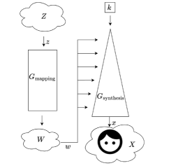
Fig. 1: The StyleGAN architecture summarised, $k$ is a constant learned during training.

In the latent space $W$ defined as $w\in W,G_{\text{mapping}}(z)=w$, significant semantic directions have already been found [16], [17].The space $W$ fits the criteria of a good support for the projected data: we already know there is a function from it to the face image space, and it has low cardinality.

To invert suspicious frames in the latent space of StyleGAN, we have to go through an optimisation process, as the generator is highly non-linear and complex. Many solutions exist for this task, such as proposed by [4] [18] [19] and [20]. Most of these solutions are based on gradient descent-algorithms to minimise a loss such as $L(w)=L_{p}(G_{\text{synthesis}}(w),x)+\alpha||G_{\text{synthesis}}(w)-x||_{2}^{2}$, with $L_{p}$ a neural distance such as LPIPS [21]. Once we are satisfied with the projection, we can discriminate out-of-distribution codes as deepfakes. Each dimensionality reduction method $P$ takes a $256\times 256$ pixels RGB image as an input and produces a low-dimensionality code. In this study the PCA models have been fitted according to the Incremental PCA algorithm [22], the code is the result of keeping the $512$ most important dimensions of the image projected in the PCA space, $P_{\text{PCA}}:\mathbb{R}^{512\times 512\times 3}\to\mathbb{R}^{512}$. For the VAE, the Vector-Quantized Variational AutoEncoder 2 (VQ-VAE-2) [23] has been chosen because of its performance. After passing the image through the encoder, the resulting latent variables (indices in the VQ-VAE-2 codebook) which are used normally by the decoder, are the chosen codes. The VQ-VAE projector $P_{\text{VQ-VAE-2}}:\mathbb{R}^{512\times 512\times 3}\to\mathbb{N}^{512\times 10}$ is effectively the encoder part of the network. Finally, a StyleGAN inversion which follows [19] is chosen. A first code is obtained from the input image thanks to an encoder $E_{\text{domain}}$, it is then optimised by gradient descent for a hundred steps. The resulting projector can be described as $P_{\text{StyleGAN}}:\mathbb{R}^{512\times 512\times 3}\to\mathbb{R}^{512\times 14}$. This process is represented in Figure 2. Each of these projectors was taken pretrained ($P_{\text{PCA}}$ was fitted) on the Flickr-Faces-HQ-256 dataset [4]. Ideally, discriminating real and fake images is easier in the latent space associated with the different projectors $P_{\text{PCA}},P_{\text{VQ-VAE-2}}\text{ and }P_{\text{SyleGAN}}$, as illustrated in Figure 3.

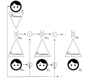
Fig. 2: The StyleGAN pseudo-inversion process. The initialisation is made with the encoder $E_{\text{domain}}$. The resulting latent code is then optimised with $L$ calculated between the reconstruction and the original image.

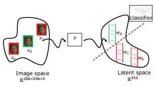
Fig. 3: Data separation is easier after a pass through the projector $P$.

4 Experiments

Binary classification models are trained to determine whether or not a low-dimensionality code is from a deepfake frame. Given the dimensionality of the inputs, using classical machine learning models was the sensible choice for discrimination models. A Random Forest classifier [11] (RF), simple Multi-Layer Perceptrons (MLP) and a logistic regression have been tested for this task. Other models (Support Vector Machines, Gaussian Mixture Models) were tested but their performance (either accuracy or training time) were not the most satisfactory.

Different combinations of projectors and classifiers are compared to state-of-the-art deepfake classifiers (MesoNet[2], XCeptionNet[3] and EfficientNet[24]) on the DFDC database [7]. Lastly, as the different channels of the StyleGAN latent code have different impacts on the generation result, a study on their relative importance is made.

4.1 Data preparation

The proposed method allows for a shorter training duration given the same data (the more complex models, such as StyleGAN and the encoder used by Zhu et al. [19] are pretrained and frozen). However the inference process as a whole is slowed down by the inversion of each image in the latent space of StyleGAN (about 25 seconds on a NVIDIA QUADRO RTX 3000, and about 2-3 seconds on a NVIDIA A100), or, to a smaller extent, the inference of the VQ-VAE-2 encoder or the projection by the PCA model. As a consequence, one in every 10 frames was uniformly sampled throughout the videos of the DFDC dataset. This frequency was chosen to assure a relatively diverse set of faces, not too correlated to one another. Each frame was processed according to the FFHQ alignment protocol before having their dimensionality reduced. Training and testing sets were separated at the video level, the testing set was composed of around 15k frames, extracted from 301 videos. Finally, only the preview set of DFDC [25] was used for training.

4.2 Results

4.2.1 Reconstruction visualisation

Figure 4 shows two examples of face reconstruction from the low-dimensionality codes, a genuine face (top) and a deepfake (bottom). Underneath is shown the average of the VGG-based LPIPS distance [21] from the original face image taken over 250 samples.

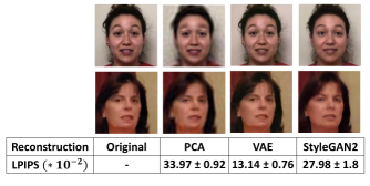
Fig. 4: Reconstruction of two faces after the dimensionality reductions, on 256px images. The top row is a genuine image, and the bottom one a deepfake.The LPIPS shown is calculated as a mean over 250 different faces, and displayed with a 95 % confidence interval.

VQ-VAE-2 offers the lowest perceptual reconstruction error, while the PCA performs the worst. StyleGAN sits in between, albeit with a higher variance, probably due to the fact that some images may need different optimisation steps to converge properly. It is to be noted that, if needed, the reconstruction fidelity of the StyleGAN method can be adjusted by cutting short or prolonging the iterative inversion process, making a compromise between quality and computing time.

4.2.2 Deepfake classification

To test if there is a dimensionality reduction method better suited for discriminating deepfakes, three instances of a Random Forest classifier [11] are trained on the codes outputted by each projector. Those classifiers were composed of 1500 estimators and were trained to optimise the Gini criterion. They were implemented using the scikit-learn package [26], with other parameters left to default. The results are shown in Table 1, with the methods labelled RF. Even if the VQ-VAE-2 (VAE) allows for the best reconstruction of its inputs (as previously shown in the Figure 4), its latent variables are in the form of discrete values referencing a codebook used by the model. While this format allows for a compact and exhaustive representation of the data, it does not contain easily accessible, discriminating information about deepfakes. To classify deepfakes, the StyleGAN (SG) projection methods obtains the best performance. Still, this analysis shows that a few thousand dimensions, instead of the hundreds of thousands usually used, can contain enough information to discriminate genuine images from deepfakes to a satisfactory degree. This could further motivate the progression towards a more frugal approach to deepfake classification.

To further improve the performance of the StyleGAN dimensionality reduction and Random Forest Classifer pipeline, three other alternative classifiers were tested. The first one being a simple logistic regression model (LR), the second one a simple neural network with one single hidden layer of dimension $512$ (MLP-2), and finally a five-layer neural network (MLP-5), with four hidden layers of size $2048,512,512$ and $512$. The two bigger models use the ReLU as the intermediate activation function, and they all produce a final output of size $1$ with a Sigmoid activation function. The logistic regression model and the neural networks are trained by optimizing the binary cross-entropy. The models were implemented in PyTorch [27], and were optimised with Stochastic Gradient Descent and a learning step of $5.10^{-4}$. The proposed methods are compared with the state-of-the-art deepfake detection methods MesoNet[2], XCeptionNet[3] and EfficientNet[24] which were taken pretrained on the complete DFDC database [7], and tested on the same examples as the proposed method.

Training Set (# Videos)	Method	Accuracy
DFDC (124k)	MesoNet	0.84
	XCeptionNet	0.91
	EfficientNet	0.91
DFDC Preview (5k)	Ours (PCA RF)	0.78
	Ours (VAE RF)	0.69
	Ours (SG RF)	0.88
	Ours (SG LR)	0.92
	Ours (SG MLP-2)	0.93
	Ours (SG MLP-5)	0.94

Table 1: Deepfake classification accuracy, best performance is in bold.

As can be seen from the binary classification accuracy results in Table 1, the proposed methods can achieve comparable or better performances than other state-of-the-art models. In particular, the proposed method with the RandomForest Classifier performs better than MesoNet ($+4\%$ of accuracy), another model designed to be light. Accuracy can be further improved by using a simple logistic regression classifier instead of the RadomForest one (another improvement of $4\%$ in terms of accuracy). The best performance is obtained by combining the StyleGAN dimensionality reduction and the MLP classifiers (SG MLP-2 and SG MLP-5), outperforming the other models by a noticeable margin, including the state-of-the-art XCeptionNet and EfficientNet methods.

4.2.3 Training dataset size

The first column of Table 1 shows the amount of videos the models were trained on. Around 25 times fewer deepfake videos were used to train the proposed models compared to the other off-the-shelf models. An advantage of using dimensionality reduction is the reduced training time, and the lesser need for data compared to other state-of-the-art methods, making it preferable when efficiency is required or when little labelled data is available (e.g. when a new modification method arrives). The proposed method is, as such, best suited for small scale scenarios such as when dealing with personal threats, or blackmail on an individual level.

4.2.4 Importance across the different channels of the latent space

Originally, StyleGAN pseudo-inversion was accomplished by optimising the single vector $w\in\mathbb{R}^{512}$ which was then fed at different stages of the generation process to compute the desired image [4]. It was also found that starting the generation process with a first latent code $w_{1}$ and finishing it with another $w_{2}$ resulted in a style mixing of facial features. The first generation steps corresponding to coarser (e.g. head shape, age) features and the latter to finer features (e.g. hair colour). A more visual explanation on feature mixing is available in the original paper [4]. Meanwhile, when designing higher-fidelity optimisation processes, researchers found that duplicating the latent code in multiple channels and optimising accross them differently yielded better results [18].

In the proposed method, the inversion process of StyleGAN by Zhu et al. [19] produces a latent code $w$ optimised along 14 channels. It was tested whether or not individual channels had a different impact on classification accuracy. Figure 5 shows the performance of different instances of the same model trained separately on each channel. Each model (MLP-5 and RF) was trained under the same conditions (hyper-parameters and data) as in the previous experiments.

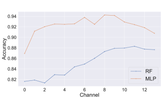
Fig. 5: Deepfake detection accuracy with the Random Forest classifier and MultiLayer Perceptron (5 layers) across different channels of StyleGAN latent code $w$.

The mid-to-late layers (8-11 with the chosen methods) are more useful in deepfake detection than the early ones. Indeed, theoretically perfect deepfake generation can be seen as keeping both the original face’s coarsest (e.g. head shape and age) and finest (e.g. hairstyle and skin texture) features, while changing the ones responsible for expression. Still, RandomForest Classifiers and MultiLayer Perceptrons do not provide their best accuracy on the same channels (9-10-11 for the RF, and 6-8-9 for the MLP). This finding may help in improving the performance and explainability of deepfake detectors in the future.

5 Conclusion

We proposed a lightweight deepfake classifier which is able to outperform complex state-of-the-art models with fewer training examples. On top of making deepfake detection more accessible, the proposed approach shows how focusing on key information in the data can help progressing towards more frugal deepfake detectors. It could be interesting in the future to look more closely at other low-dimensionality spaces, in particular other inversion variants for the StyleGAN framework which are already promising.

References

- [1] Yann LeCun, Bernhard Boser, John S Denker, Donnie Henderson, Richard E Howard, Wayne Hubbard, and Lawrence D Jackel, “Backpropagation applied to handwritten zip code recognition,” Neural computation, vol. 1, no. 4, pp. 541–551, 1989.
- [2] Darius Afchar, Vincent Nozick, Junichi Yamagishi, and Isao Echizen, “Mesonet: a compact facial video forgery detection network,” in 2018 IEEE international workshop on information forensics and security (WIFS). IEEE, 2018, pp. 1–7.
- [3] François Chollet, “Xception: Deep learning with depthwise separable convolutions,” in Proceedings of the IEEE conference on computer vision and pattern recognition, 2017, pp. 1251–1258.
- [4] Tero Karras, Samuli Laine, and Timo Aila, “A style-based generator architecture for generative adversarial networks,” in Proceedings of the IEEE/CVF conference on computer vision and pattern recognition, 2019, pp. 4401–4410.
- [5] Jun-Yan Zhu, Taesung Park, Phillip Isola, and Alexei A Efros, “Unpaired image-to-image translation using cycle-consistent adversarial networks,” in Proceedings of the IEEE international conference on computer vision, 2017, pp. 2223–2232.
- [6] Andreas Rossler, Davide Cozzolino, Luisa Verdoliva, Christian Riess, Justus Thies, and Matthias Nießner, “Faceforensics++: Learning to detect manipulated facial images,” in Proceedings of the IEEE/CVF International Conference on Computer Vision, 2019, pp. 1–11.
- [7] Brian Dolhansky, Joanna Bitton, Ben Pflaum, Jikuo Lu, Russ Howes, Menglin Wang, and Cristian Canton Ferrer, “The deepfake detection challenge (dfdc) dataset,” arXiv preprint arXiv:2006.07397, 2020.
- [8] Shruti Agarwal, Hany Farid, Tarek El-Gaaly, and Ser-Nam Lim, “Detecting deep-fake videos from appearance and behavior,” in 2020 IEEE International Workshop on Information Forensics and Security (WIFS). IEEE, 2020, pp. 1–6.
- [9] Davide Cozzolino, Andreas Rössler, Justus Thies, Matthias Nießner, and Luisa Verdoliva, “Id-reveal: Identity-aware deepfake video detection,” in Proceedings of the IEEE/CVF International Conference on Computer Vision, 2021, pp. 15108–15117.
- [10] Erich Leo Lehmann, Joseph P Romano, and George Casella, Testing statistical hypotheses, vol. 3, Springer, 2005.
- [11] Leo Breiman, “Out-of-bag estimation,” 1996.
- [12] R. Bellman, Rand Corporation, and Karreman Mathematics Research Collection, Dynamic Programming, Rand Corporation research study. Princeton University Press, 1957.
- [13] Karl Pearson, “Liii. on lines and planes of closest fit to systems of points in space,” The London, Edinburgh, and Dublin philosophical magazine and journal of science, vol. 2, no. 11, pp. 559–572, 1901.
- [14] Mark A Kramer, “Nonlinear principal component analysis using autoassociative neural networks,” AIChE journal, vol. 37, no. 2, pp. 233–243, 1991.
- [15] Diederik P Kingma and Max Welling, “Auto-encoding variational Bayes,” in Int. Conf. on Learning Representations.
- [16] Yujun Shen, Jinjin Gu, Xiaoou Tang, and Bolei Zhou, “Interpreting the latent space of gans for semantic face editing,” in Proceedings of the IEEE/CVF conference on computer vision and pattern recognition, 2020, pp. 9243–9252.
- [17] Erik Härkönen, Aaron Hertzmann, Jaakko Lehtinen, and Sylvain Paris, “Ganspace: Discovering interpretable gan controls,” Advances in Neural Information Processing Systems, vol. 33, pp. 9841–9850, 2020.
- [18] Rameen Abdal, Yipeng Qin, and Peter Wonka, “Image2stylegan: How to embed images into the stylegan latent space?,” in Proceedings of the IEEE/CVF International Conference on Computer Vision, 2019, pp. 4432–4441.
- [19] Jiapeng Zhu, Yujun Shen, Deli Zhao, and Bolei Zhou, “In-domain gan inversion for real image editing,” in European conference on computer vision. Springer, 2020, pp. 592–608.
- [20] Weihao Xia, Yulun Zhang, Yujiu Yang, Jing-Hao Xue, Bolei Zhou, and Ming-Hsuan Yang, “Gan inversion: A survey,” IEEE Transactions on Pattern Analysis and Machine Intelligence, 2022.
- [21] Richard Zhang, Phillip Isola, Alexei A Efros, Eli Shechtman, and Oliver Wang, “The unreasonable effectiveness of deep features as a perceptual metric,” in CVPR, 2018.
- [22] David A Ross, Jongwoo Lim, Ruei-Sung Lin, and Ming-Hsuan Yang, “Incremental learning for robust visual tracking,” International journal of computer vision, vol. 77, no. 1, pp. 125–141, 2008.
- [23] Ali Razavi, Aaron Van den Oord, and Oriol Vinyals, “Generating diverse high-fidelity images with vq-vae-2,” Advances in neural information processing systems, vol. 32, 2019.
- [24] Mingxing Tan and Quoc Le, “Efficientnet: Rethinking model scaling for convolutional neural networks,” in International conference on machine learning. PMLR, 2019, pp. 6105–6114.
- [25] Brian Dolhansky, Russ Howes, Ben Pflaum, Nicole Baram, and Cristian Canton Ferrer, “The deepfake detection challenge (dfdc) preview dataset,” arXiv preprint arXiv:1910.08854, 2019.
- [26] F. Pedregosa, G. Varoquaux, A. Gramfort, V. Michel, B. Thirion, O. Grisel, M. Blondel, P. Prettenhofer, R. Weiss, V. Dubourg, J. Vanderplas, A. Passos, D. Cournapeau, M. Brucher, M. Perrot, and E. Duchesnay, “Scikit-learn: Machine learning in Python,” Journal of Machine Learning Research, vol. 12, pp. 2825–2830, 2011.
- [27] Adam Paszke, Sam Gross, Francisco Massa, Adam Lerer, James Bradbury, Gregory Chanan, Trevor Killeen, Zeming Lin, Natalia Gimelshein, Luca Antiga, Alban Desmaison, Andreas Kopf, Edward Yang, Zachary DeVito, Martin Raison, Alykhan Tejani, Sasank Chilamkurthy, Benoit Steiner, Lu Fang, Junjie Bai, and Soumith Chintala, “Pytorch: An imperative style, high-performance deep learning library,” in Advances in Neural Information Processing Systems 32, pp. 8024–8035. Curran Associates, Inc., 2019.