Real space analysis for edge burst in a non-Hermitian quntum walk model

Abstract

Edge burst is a novel phenomenon in non-Hermitian quantum dynamics discovered by a very recent numerical study [W.-T. Xue, et al, Phys. Rev. Lett 2, 128.120401(2022)]. It finds that a large proportion of particle loss occurs at the system boundary in a class of non-Hermitian quantum walk. In this paper, we investigate the evolution of real-space wavefunction for this lattice system. We find the wavefunction of the edge site is distinct from the bulk sites. By introducing the time-dependent perturbation theory, we evaluate the analytical expression of the real-space wavefunctions and find the different evolution behavior between the edge site and bulk sites originates from their different nearby sites configuration. The main contribution of the edge wavefunction originates from the transition of the two adjacent non-decay sites. Besides, the numerical diagonalization shows the edge wavefunction is mainly propagated by a group of eigen-modes with a relatively large imaginary part. Our work provides an analytical method for studying non-Hermitian quantum dynamical problems in real space.

I INTRODUCTION

The Hermiticity of Hamiltonian is a fundamental requirement for a closed system in quantum physics Shankar (2012). In many situations, however, one is only interested in a limited subspace of the whole system, and it can be encapsulated in an effective non-Hermtian Hamiltonian El-Ganainy et al. (2018); Ashida et al. (2020). Such systems include but are not limited to optical systems with gain and loss Makris et al. (2008); Klaiman et al. (2008); Guo et al. (2009); Rudner and Levitov (2009); Longhi (2009); Chong et al. (2011); Regensburger et al. (2012); Bittner et al. (2012); Liertzer et al. (2012); Feng et al. (2014); Hodaei et al. (2014), open systems with dissipation Carmichael (1993); Rotter (2009); Choi et al. (2010); Lin et al. (2011); Lee and Chan (2014); Malzard et al. (2015); Yamamoto et al. (2019); Li et al. (2019), and electron systems with finite-lifetime quasiparticles Zyuzin and Zyuzin (2018); Shen and Fu (2018); Yoshida et al. (2018); Zhou et al. (2018); Papaj et al. (2019); Kimura et al. (2019). Another important class of non-Hermitian systems is provided by lattices, where the role of topology has attracted tremendous interest Lee (2016); Leykam et al. (2017); Gong et al. (2018); Shen et al. (2018); Kunst et al. (2018); Yao et al. (2018); Yao and Wang (2018); Martinez Alvarez et al. (2018); Lee and Thomale (2019); Lee et al. (2019a); Longhi (2019a); Zhou and Lee (2019); Liu et al. (2019a); Edvardsson et al. (2019); Song et al. (2019a, b); Yokomizo and Murakami (2019); Zhang et al. (2019); Jin and Song (2019); Liu et al. (2019b); Ghatak and Das (2019); Kawabata et al. (2019); Herviou et al. (2019); Borgnia et al. (2020); Longhi (2019b); Kunst and Dwivedi (2019); Imura and Takane (2019); Okuma and Sato (2019); Lee et al. (2019b); Longhi (2019c); Okuma et al. (2020); Yi and Yang (2020); Kawabata et al. (2020a); Zhang and Gong (2020); Kawabata et al. (2020b); Longhi (2020a); Zhang et al. (2020); Yang et al. (2020); Matsumoto et al. (2020); Lee and Longhi (2020); Li et al. (2020); Fu et al. (2021); Okugawa et al. (2020); Longhi (2020b); Liu et al. (2020); Edvardsson et al. (2020); Gao et al. (2020); Xiao et al. (2020); Ghatak et al. (2020); Helbig et al. (2020); Hofmann et al. (2020); Weidemann et al. (2020); Song et al. (2020); Torres (2019); Bergholtz et al. (2021); Wang et al. (2021a); Hu and Zhao (2021); Yokomizo and Murakami (2021a); Okuma and Sato (2021a); Zirnstein et al. (2021); Claes and Hughes (2021); Okuma and Sato (2021b); Kawabata et al. (2021); Guo et al. (2021); Sun et al. (2021); Haga et al. (2021); Wang et al. (2021b); Xue et al. (2021); Okugawa et al. (2021); Lin et al. (2021); Longhi (2021a); Yokomizo and Murakami (2021b); Longhi (2021b); Wang et al. (2021c, d); Zhang et al. (2022); Wu et al. (2022); Weidemann et al. (2022); Lin et al. (2022); Longhi (2022); Faugno and Ozawa (2022); Li et al. (2022); Zhu and Gong (2022). A unique feature of non-Hermitian lattices is the non-Hermitian skin effect (NHSE), namely the localization of an enormous number of bulk-band eigenstates at the edges under open boundary conditions Yao and Wang (2018); Martinez Alvarez et al. (2018); Lee and Thomale (2019); Lee et al. (2019a); Longhi (2019a); Okuma et al. (2020); Yi and Yang (2020); Kawabata et al. (2020a); Liu et al. (2020); Okuma and Sato (2021b); Sun et al. (2021); Claes and Hughes (2021); Guo et al. (2021); Kawabata et al. (2021). A significant consequence of NHSE is the breakdown of the conventional bulk-boundary correspondence, which can be recovered by using the localized skin modes replacing the extended Bloch waves of Hermitian lattices Kunst et al. (2018); Yao et al. (2018); Yao and Wang (2018); Song et al. (2019a); Helbig et al. (2020); Xiao et al. (2020); Ghatak et al. (2020); Bergholtz et al. (2021). It indicates that the boundary is even more important in non-Hermitian physics compared to their Hermitian counterparts.

Recently, a novel boundary-induced dynamical phenomenon named ”edge burst” is reported in the Ref Xue et al. (2022) and the experimental verification is reported in the Ref Xiao et al. (2023). When a quantum particle (called ”quantum walker”) walks freely in a class of lossy lattices, it is intuitively expected that the decay probability is dominated by the lossy sites near the initial location of the walker. Surprisingly, the numerical study finds that there is an unexpected remarkable loss probability peak at the edge, with an almost invisible loss probability tail in the bulk Xue et al. (2022). The appearance of such an edge peak has also been reported in an earlier work with an incorrect explanation Wang et al. (2021a), which is based on topology. Although previous work have investigated the edge burst phenomenon, however, the relation between the real space dynamical behavior of the system and the formation of this burst peak is still unconscious.

In this work, we investigate the dynamical evolution of quantum particles in a lossy lattice. The numerical simulation shows the edge burst phenomenon is closely related to the distinct dynamical behavior of wavefunctions between the edge and bulk sites. To further understand how the walker propagates in the lattice, we introduce time-dependent perturbation theory for non-Hermitian systems and evaluate the analytical expression of the real-space quantum walk wavefunctions. Due to the NHSE, the walker mainly hops nonreciprocally along the non-decay chain. The analysis of real-space wavefunctions shows the different evolution features between the edge and bulk can be attributed to their nearby site configuration, which limits the possible path the walker can travel from the initial state. Besides, we find that the main contribution to the edge wavefunction originates from the interference transition of the two adjacent non-decay sites. Furthermore, we discuss the relation between the evolution of the system and its eigen-modes by numerical diagonalization. The result shows the walker is mainly propagated by a group of eigen-modes which have a large imaginary part when it arrives at the edge, which is irrelevant to the topological eigen-modes. Our work gives an explicit illustration of the edge burst phenomenon in real space and provides an alternative method to investigate non-Hermitian dynamical problems.

This paper is organized as follows. We introduce the non-Hermitian quantum walk model and describe the edge burst phenomenon with numerical simulations in Sec. II. A sketch of time-dependent perturbation theory for non-Hermitian Hamiltonian is given in Sec. III. We apply the theory in the concrete quantum walk model and solve the evolution equation analytically in Sec. IV. By the analysis of wavefunction, we elucidate the propagation process of the walker and the formation of edge burst in real space directly. In Sec. V, we disscuss the relation between the evolution of the edge wavefunction and the eigenstates of the system. Finally, a summary is given in Sec. VI.

II Model and non-Hermitian Edge Burst

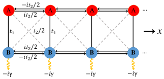
Figure 1: Schematic diagram of the non-Hermitian lattice. Each unit cell, labeled by spatial coordinate $x$, contains two sites A and B.

Let’s consider a one-dimensional non-Hermitian lattice (see Fig. 1), from which the walker can escape during the quantum walk. The state of the system $\left|\psi\right\rangle$ evolves according to the following equations of motion (we set $\hbar=1$):

$$i\frac{d\psi_{x}^{A}}{dt}=t_{1}\psi_{x}^{B}+i\frac{t_{2}}{2}\left(\psi_{x-1}^{A}-\psi_{x+1}^{A}\right)+\frac{t_{2}}{2}\left(\psi_{x-1}^{B}+\psi_{x+1}^{B}\right),$$

$$i\frac{d\psi_{x}^{B}}{dt}=t_{1}\psi_{x}^{A}-i\frac{t_{2}}{2}\left(\psi_{x-1}^{B}-\psi_{x+1}^{B}\right)+\frac{t_{2}}{2}\left(\psi_{x-1}^{A}+\psi_{x+1}^{A}\right)$$

$$\ \ \ \ \ \ \ \ \ \ -i\gamma\psi_{x}^{B},$$ (1)

where $\psi_{x}^{A}=\left\langle x,A|\psi\right\rangle$ and $\psi_{x}^{B}=\left\langle x,B|\psi\right\rangle$ are the amplitudes of the walker on the sublattices A and B at the site $x$. Without loss of generality, We choose the hopping amplitude parameters $t_{1}$ and $t_{2}$ to be real numbers. The onsite imaginary potential $-i\gamma$ describe the loss particles on B sites with rate $2\gamma$. This model differs from previous quantum work model Rudner and Levitov (2009), as it features the NHSE. This can be seen clearly by mapping a similar model in Ref. Lee (2016), to the non-Hermitian Su-Schrieffer-Heeger (SSH) model with nonreciprocal hopping Yao and Wang (2018). The mathematical relation of these lattice models can be seen in Appendix A.

For a general Hamiltonian $\mathcal{\hat{H}}=\hat{H}-i\hat{\Gamma},$ where $\hat{H}$ and $\hat{\Gamma}$ are Hermitian operators, the norm of a quantum state $\left|\psi\right\rangle$ evolves according to $\frac{d}{dt}\left\langle\psi|\psi\right\rangle=-2\left\langle\psi\left|\hat{\Gamma}\right|\psi\right\rangle.$ In the non-Hermitian quantum walk model we consider, the system decays according to$\frac{d}{dt}\left\langle\psi|\psi\right\rangle=-\sum_{x}2\gamma\left|\psi_{x}^{B}\right|^{2},$ and the local decay probability on site $x$ is

$$P_{x}=\int_{0}^{\infty}2\gamma\left|\psi_{x}^{B}\left(t\right)\right|^{2}dt.$$ (2)

If the initial state $\left|\psi\left(0\right)\right\rangle$ is normalized, the decay probability distribution satisfies $\sum_{x}P_{x}=1$. Now, suppose a walker starts from some sublattice A of site $x$ at time $t=0,$ namely $\psi_{x}^{A}\left(0\right)=\delta_{x,x_{0}},\psi_{x}^{B}\left(0\right)=0,$ and involve freely under the equations of motion (1). The hop between different sites drives the walker away from $x_{0},$ and during this quantum walk, the walker can escape from any B sites. This can be seen clearly in Fig. 2(a) and 2(b), which is the numerical solution of $P_{x}.$ The distribution of $P_{x}$ is left-right asymmetric and it originates from the non-Hermitian skin effect, the walker tends to jump towards left as all eigenstates are localized at the left edge.

A fascinating property of the system is the edge burst Xue et al. (2022), namely the appearance of a prominent peak in the loss probability at the edge, with the nearby almost invisible decaying tail (see Fig. 2(a)). Such an unexpected peak was numerically seen in the earlier Ref. Wang et al. (2021a) and it was attributed to topological edge states. This interpretation was regarded as wrong in Xue et al. (2022) for the disappearance of the high peak in the topological nontrivial region. To explore how the walker propagates in the lattice and form a burst loss probability peak at the edge, we focus on the time evolution of $\psi_{x}^{B}.$ The numerical calculation shows that $\psi_{x}^{B}$ are purely imaginary. Furthermore, when there is the edge burst phenomenon, the dynamical evolution of wavefunction at the edge is distinct from the bulk one. We can see this clearly in Fig. 2(c) that $\psi_{1}^{B}$ have a tremendous large increased amplitude peak after the first tiny peak, while other $\psi_{x\neq 1}^{B}$ oscillates with a decreasing amplitude as t becomes larger. This interesting feature is crucial to form a burst edge peak. There is no such tremendous large increased peak for $\psi_{1}^{B}$ in Fig. 2(d), where all $\psi_{x}^{B}$ have the same decreased oscillation behavior, and the corresponding edge loss probability $P_{1}$ in Fig. 2(b) is very small.

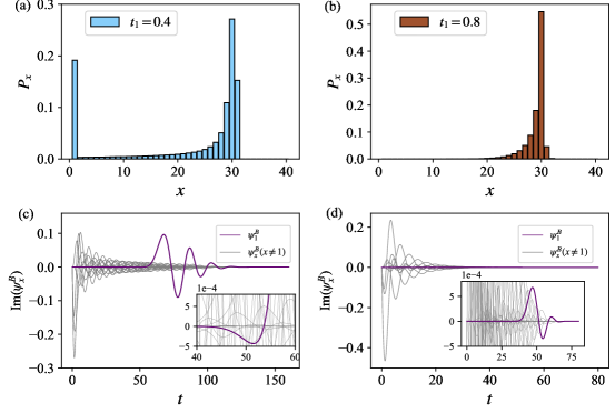
Figure 2: (a),(b) The spatially resolved loss probability $P_{x}$ for a walker initiated at $x_{0}=30$. $t_{1}=0.4$ for (a) and $t_{1}=0.8$ for (b). The chain length $L=40$. (c),(d) The corresponding time evolution of $\psi_{x}^{B}$ to (a),(b) respectively. The common parameters $t_{2}=0.5$, $\gamma=0.8$ are fixed throughout (a)–(d).

III Non-Hermitian time-dependent perturbation theory

We can get the analytical expression of $\psi_{x}^{B}\left(t\right)$ via time-dependent perturbation theory. The sketch of this theory is encapsulated as follows. We consider a non-Hermitian Hamiltonian $\hat{H}\left(t\right)$ such that it can be split into time-independent part $\hat{H}_{0}$ and time-dependent part $\hat{H}^{\prime}\left(t\right)$, namely

$$\hat{H}\left(t\right)=\hat{H}_{0}+\hat{H}^{\prime}\left(t\right),$$ (3)

and the corresponding Schrödinger equation is

$$i\frac{\partial}{\partial t}\left|\Psi\left(t\right)\right\rangle=\hat{H}\left(t\right)\left|\Psi\left(t\right)\right\rangle.$$ (4)

When $\hat{H}^{\prime}\left(t\right)=0$, Eq. (4) can be solved if we know the solution of eigen-equations $\hat{H}_{0}\left|n\right\rangle=E_{n}\left|n\right\rangle$ with eigenstates $\left|n\right\rangle$ and eigenvalues $E_{n}$, that is

$$\left|\Psi\left(t\right)\right\rangle=e^{-i\hat{H}_{0}t}\left|\Psi\left(0\right)\right\rangle,$$ (5)

where $\left|\Psi\left(0\right)\right\rangle$ is the linear combination of $\left|n\right\rangle$. If $\hat{H}^{\prime}\left(t\right)\neq 0,$ it is no longer a stationary problem and we are interested in the case that the initial state $\left|k\right\rangle$ is one of the eigenstates of $\hat{H}_{0}.$ Due to the perturbation of $\hat{H}^{\prime}\left(t\right),$ the state $\left|k\right\rangle$ is an unstable state. We assume the system is a superposition of the eigenstates of $\hat{H}_{0}$ for $t>0$ and given by

$$\left|\Psi\left(t\right)\right\rangle=\sum_{n}\left|\psi_{n}\left(t\right)\right\rangle=\sum_{n}c_{n}\left(t\right)e^{-iE_{n}t}\left|n\right\rangle.$$ (6)

Substituting this ansatz wavefunction into Schrödinger equation (4) and multiplying by the state $\left\langle m\right|$, we get a coupled differential equation of wavefunction expansion coefficient under unperturbed representation $\hat{H}_{0}$ as

$$i\frac{dc_{m}\left(t\right)}{dt}=\sum_{n}H_{mn}^{\prime}\left(t\right)c_{n}\left(t\right)e^{i\left(E_{m}-E_{n}\right)t},$$ (7)

where $H_{mn}^{\prime}\left(t\right)=$ $\left\langle m\right|\hat{H}^{\prime}\left(t\right)\left|n\right\rangle$. To solve the differential equation (6) with the initial condition $c_{m}\left(0\right)=\delta_{mk}$, we take the perturbation expansion of $c_{m}\left(t\right)$ and use the iteration method. Specifically, $c_{m}\left(t\right)$ can be written as

$$c_{m}\left(t\right)=c_{m}^{\left(0\right)}+c_{m}^{\left(1\right)}+c_{m}^{\left(2\right)}+\cdots,$$ (8)

where $c_{m}^{\left(1\right)},~{}c_{m}^{\left(2\right)},~{}\cdots$ signify amplitudes of the first order, second order, and so on in the strength parameter of time-dependent Hamiltonian. Plugging Eq. (8) into Eq. (7) and comparing the order of perturbation, we can get the $l$ th-order equation:

$$i\frac{d}{dt}c_{m}^{\left(l\right)}\left(t\right)=\sum_{n}H_{mn}^{\prime}\left(t\right)c_{n}^{\left(l-1\right)}\left(t\right)e^{i\left(E_{m}-E_{n}\right)t},$$ (9)

This equation can be solved easily by integrating it directly if we know all of $(l-1)$ th-order solutions $c_{n}^{\left(l-1\right)}$. Thus, we can solve Eq. (7) step by step and the solution up to $l$ th-order is

$$c_{m}\left(t\right)\simeq c_{m}^{\left(0\right)}\left(t\right)+c_{m}^{\left(1\right)}\left(t\right)+\cdots+c_{m}^{\left(l\right)}\left(t\right).$$ (10)

It should be noticed that this approximate solution has a convergent radius $t_{0}$, which is related to the perturbation expansion order and the strength parameters of perturbation.

IV Burst peak from time-dependent theory

For the non-Hermitian quantum walk model, we set the onsite potential operator as the unperturbed Hamiltonian $\hat{H}_{0}$ and its real-space matrix elements are $\left\langle x,s\right|\hat{H}_{0}\left|x^{\prime},s^{\prime}\right\rangle=-\frac{i\gamma}{2}\delta_{xx^{\prime}}\delta_{ss^{\prime}}\left[1-\left(\sigma_{z}\right)_{ss^{\prime}}\right],$ with $x,x^{\prime}$ referring to the location of the unit cell and $s,s^{\prime}=A,B$ referring to the sublattice label. The eigen-equation is $\hat{H}_{0}\left|x,s\right\rangle=E_{x}^{s}\left|x,s\right\rangle$, with two $N$-fold eigenvalues $E_{x}^{A}=0$ and $E_{x}^{B}=-i\gamma$ respectively. The hopping of the walker is treated as the perturbation operator $\hat{H}^{\prime}$ and its matrix elements are $H_{xs,x^{\prime}s^{\prime}}^{\prime}=\left\langle x,s\left|\hat{H}^{\prime}\right|x^{\prime},s^{\prime}\right\rangle$. Thus, according to the perturbation procedure in Sec. III, we can evaluate the evolution of the amplitude of the walker on any site. Specifically, Eq. (7) will be reduced to

$$i\frac{dc_{x}^{s}\left(t\right)}{dt}=\sum_{x^{\prime}s^{\prime}}H_{xs,x^{\prime}s^{\prime}}^{\prime}c_{x^{\prime}}^{s^{\prime}}\left(t\right)e^{i\left(E_{x}^{s}-E_{x^{\prime}}^{s^{\prime}}\right)t}.$$ (11)

One can integrate both sides of this equation and get the formal solution,

$$c_{x}^{s}\left(t\right)=-i\sum_{x^{\prime}s^{\prime}}\int_{0}^{t}H_{xs,x^{\prime}s^{\prime}}c_{x^{\prime}}^{s^{\prime}}\left(t^{\prime}\right)e^{i\left(E_{x}^{s}-E_{x^{\prime}}^{s^{\prime}}\right)t^{\prime}}dt^{\prime}.$$ (12)

with the relation $\psi_{x}^{s}\left(t\right)=e^{-iE_{x}^{s}t}c_{x}^{s}\left(t\right),$ the formal solution can be written as the relation between the amplitude of the different sites:

$$\psi_{x}^{s}\left(t\right)=-ie^{-iE_{x}^{s}t}\sum_{x^{\prime}s^{\prime}}\int_{0}^{t}e^{iE_{x}^{s}t^{\prime}}H_{xs,x^{\prime}s^{\prime}}\psi_{x^{\prime}}^{s^{\prime}}\left(t^{\prime}\right)dt^{\prime}.$$ (13)

Under the initial condition $\psi_{x}^{A}\left(0\right)=\delta_{x,x_{0}}$ and $\psi_{x}^{B}\left(0\right)=0,$ we find that the amplitudes $\psi_{x}^{A}\left(t\right)$ are always real while $\psi_{x}^{B}\left(t\right)$ are purely imaginary, which can be deduced by the perturbation process (see Appendix B). Alternatively, one can check this conclusion through the iterate equation (13). For example, if the sublattice label $s=A,$ the nonzero factors $H_{xs,x^{\prime}s^{\prime}}\psi_{x^{\prime}}^{s^{\prime}}\left(t^{\prime}\right)$ are imaginary under the assumption that $\psi_{x^{\prime}}^{s^{\prime}}\left(t^{\prime}\right)$ are real for $s^{\prime}=A$ and imaginary for $s^{\prime}=B.$ The amplitudes $\psi_{x}^{A}\left(t\right)$ thus keep real, which is a self-consistent result for equation (13).

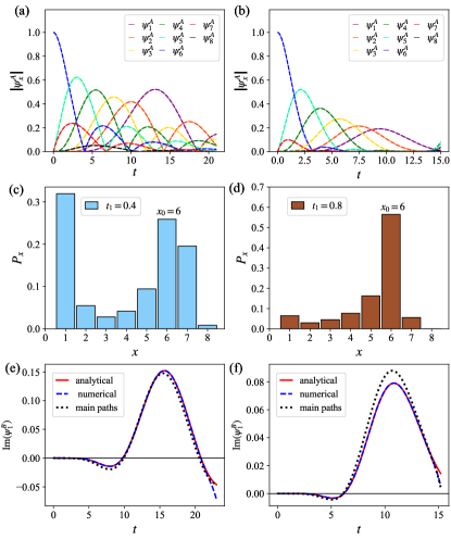
Figure 3: The wavefunctions $\psi_{x}^{A}\left(t\right)$ for a walker initiated at $x_{0}=6$. $t_{1}=0.4$ for (a) and $t_{1}=0.8$ for (b). The chain length $L=8$. (c),(d) The corresponding The spatially resolved loss probability $P_{x}$ to (a),(b) respectively. (e) and (f) are the edge wavefunctions $\psi_{1}^{B}\left(t\right)$, the evaluation of both analytical and main paths are up to 40th-order perturbation. The common parameters $t_{2}=0.5$, $\gamma=0.8$ are fixed throughout (a)–(f).

For concreteness, we consider an $8$-site lattice, and the walker is initially prepared on sublattice $A$ of site $6$. The evolution of the wavefunctions $\psi_{x}^{s}\left(t\right)$ is evaluated analytically by the perturbation theory. It finds that the dynamical behavior of the walker along the $A$ chain is crucial to forming a remarkable loss peak at the edge. For the fixed parameters $t_{2}$ and $\gamma,$ the coupling between the chain $A$ and $B$ become strong as the hopping $t_{1}$ increased, which accelerates the dissipation of the walker. In other words, the travel time of the walker along the $A$ chain becomes short. This can be seen clearly from Fig. 3(a) and 3(b), when the walker arrives at $x$, the $\psi_{x}^{A}\left(t\right)$ have smaller amplitudes and converge to zero more quickly for larger $t_{1}$. Another perspective to see this is that the dissipation probabilities $P_{x}$ near the initial location is larger as $t_{1}$ increases (see Fig. 3(c) and 3(d)). On the other hand, this non-Hermitian lattice model features the NHSE, namely the exponential localization of all eigenstates at the edge, which is characterized by the generalized Bloch factor $\beta$ with $\left|\beta\right|=\sqrt{\left|\left(t_{1}-\gamma/2\right)/\left(t_{1}+\gamma/2\right)\right|}$. In the case $\left|\beta\right|<1$ for $t_{1}>0,$ all skin modes are localized at the left edge. The NHSE induces leftward walking along the $A$ chain and the walker becomes trapped at the boundary once it arrives at $A_{1}$, which leads to the Rabi-like oscillation between sublattice $A_{1}$ and $B_{1}$. The value of the edge loss probability is dominated by the asymmetrical hop parameter $\beta$ and the dissipation of the walker during the travel to the edge. The accurate decay law in the bulk can be captured by the non-Hermitian Green function method Xue et al. (2022, 2021).

The complete analytical expression of $\psi_{x}^{s}\left(t\right)$ can be regarded as the sum of all possible physical paths the walker travels from the initial state $\left|x_{0},A\right\rangle$ to the state $\left|x,s\right\rangle$ during the time interval $t$. For example, there are only one path $\left|x_{0},A\right\rangle$ that the walker can travel to the $\left|x_{0},B\right\rangle$ by a single-step quantum jump and four paths by a two-step quantum jump, which corresponds to the first-order and second-order perturbation contribution in $\psi_{x_{0}}^{B}\left(t\right)$, respectively. We can classify every perturbation process by its final-step quantum jump. The sum of all perturbation terms with the same final-step quantum jump is the total transition amplitude from a certain nearby site of $\left|x,s\right\rangle$ to $\left|x,s\right\rangle$. This is the physical interpretation of the integral formula (13). An obvious example is the single-step quantum jump $\left|x_{0},A\right\rangle\rightarrow$ $\left|x_{0},B\right\rangle$ and the multi-step quantum jumps $\left|x_{0},A\right\rangle\rightarrow\cdots\rightarrow\left|x_{0},A\right\rangle\rightarrow$ $\left|x_{0},B\right\rangle$ belong to the same class of perturbation process. The sum of these perturbation terms is the transition amplitude from $\left|x_{0},A\right\rangle$ to $\left|x_{0},B\right\rangle$. We note that there are five such classes of perturbation processes in the bulk and three classes in the edge. Thus, the distinct evolution behavior between bulk wavefunction and edge wavefunction in edge burst phenomenon originate from the configuration of their nearby sites, which limits the possible path the walker can travel from the initial state. For example, a quantum jump process $\left|x+1,A\right\rangle\rightarrow\left|x,B\right\rangle\rightarrow\left|x-1,A\right\rangle\rightarrow\left|x,B\right\rangle$ is allowed in the bulk sites but forbidden in the edge site. Another perspective to see this is if we neglect the back transition from the two forward nearby sites, the bulk wavefunction evolves like edge wavefunction as it can be viewed as new physical edge artificially. Furthermore, we find that the edge wavefunction $\psi_{1}^{B}\left(t\right)$ can be approximated by the interference of transition amplitude from two adjacent non-decay sites $A_{1}$ and $A_{2}$, or symbolically,

$$\psi_{1}^{B}\left(t\right)\simeq-ie^{-\gamma t}\int_{0}^{t}e^{\gamma t^{\prime}}\left[t_{1}\psi_{1}^{A}\left(t^{\prime}\right)+\frac{t_{2}}{2}\psi_{2}^{A}\left(t^{\prime}\right)\right]dt^{\prime}.$$ (14)

This can be seen more clearly in Fig. 3(e) and  3(f) as we viewed the transition paths with final step quantum jumps $A_{1}$ to $B_{1}$ or $A_{2}$ to $B_{1}$ as the main paths and it fit well with analytical and numerical results. The reason is that the walker mainly propagates along the $A$ chain and the transition amplitude from $B_{2}$ site can be neglected as $\psi_{2}^{B}\left(t\right)$ is very small.

V the Eigen-modes and the edge wavefunction

Figure 4: (a) The imaginary part of an 8-site lattice. The red points at $t_{1}=0.1,t_{1}=0.4$ and $t_{1}=0.6$ corresponds to the eigenstates we choose to simulate the time evolution of $|\psi^{B}_{1}(t)|$. Other parameters are $t_{2}=0.3,\gamma=1$ and the walker is initially put at site 6A. (b) The green dashed line represents the simulation by choosing eight eigenstates with the relatively large imaginary parts of eigenvalues. The blue solid line represents the analytical solution. $t_{1}=0.1$, other parameters are the same as (a). (c) Similar to (b) except that $t_{1}=0.4$. (d) Similar to (b) except that $t_{1}=0.6$. The red dashed line represents the simulation of all sixteen eigenstates, which exactly reveals the analytical solution.

To investigate the role that different eigenstates play in the evolution process, we decompose the non-Hermitian Hamiltonian by the biorthogonal bases

$$\hat{H}=\sum_{n}E_{n}|n_{R}\rangle\langle n_{L}|,$$ (15)

where $|n_{R}\rangle$ and $\langle n_{L}|$ are the right and left eigenstates respectively and they satisfy the biorthogonal relation $\langle m_{L}|n_{R}\rangle=\delta_{mn}$ and the completeness condition $\sum_{n}|n_{R}\rangle\langle n_{L}|=\mathbb{I}$. For the non-Hermitian lattice, the state of the system evolves according to

$$|\psi(t)\rangle=e^{-i\hat{H}t}|\psi(0)\rangle,$$ (16)

where the initial state $|\psi(0)\rangle$ can be expressed by a superposition of $|n_{R}\rangle$

$$|\psi(0)\rangle=\sum_{n}a_{n}|n_{R}\rangle.$$ (17)

The coefficient $a_{n}$ is determined by the linear equations

$$\psi^{s}_{x}(0)=\sum_{n}a_{n}\phi^{s}_{n,x},$$ (18)

with $\phi^{s}_{n,x}\equiv\langle x,s|n_{R}\rangle$. Thus we can rewrite the evolution equation (16) as

$$|\psi(t)\rangle=\sum_{n}e^{-iE_{n}t}a_{n}|n_{R}\rangle.$$ (19)

Since $E_{n}={\rm Re}(E_{n})+i{\rm Im}(E_{n})$, we can rewrite the evolution equation (19) as

$$|\psi(t)\rangle=\sum_{n}e^{-i{\rm Re}(E_{n})t}e^{{\rm Im}(E_{n})t}a_{n}|n_{R}\rangle.$$ (20)

From evolution equation (20) we can see that the long time behavior of $|\psi(t)\rangle$ will be determined by the eigenstates with relatively large imaginary parts since the exponential factors in front of them decay more slowly or grow faster. So the imaginary parts of the eigenvalues play an important role in the time evolution of the wavefunction. Specifically, one can verify that the imaginary part of any eigenvalue of the system is always negative owing to the dissipation of the whole system. Moreover, the imaginary part of the eigenvalues is twofold degenerate and symmetric to $-\frac{i}{2}\gamma$, which is demonstrated in Fig.4 (a). The reason for this symmetry is that the Hamiltonian of the quantum walk $\hat{H}$ can be divided into two parts $\hat{H}=\hat{H}_{1}-\frac{i\gamma}{2}\hat{I}$ with the first part $\hat{H}_{1}$ satisfying chiral symmetry which ensures the symmetry of the eigenvalues. More details about the symmetry analysis of the Hamiltonian are given in Appendix A.

We still take this 8-site lattice as an example to show the role of the imaginary part of the eigenvalues plays in the time evolution of the wavefunction. By picking eight eigenstates with a relatively large imaginary part of eigenvalues out of all sixteen eigenstates, we simulate the evolution of the wavefunction $|\psi^{B}_{1}(t)|$ and show its result in Fig. 4(b-d). As one can see from the green dashed line in Fig. 4(b), these eight eigenstates can describe the evolution of $|\psi^{B}_{1}(t)|$ well as early as $t=5$. This is because the other eight eigenstates have much smaller imaginary parts of eigenvalues and their contribution to the wavefunction vanishes quickly. While in Fig. 4(c) with a different $t_{1}$, these eight eigenstates can fit the analytical solution well only after $t=15$, which is due to the non-negligible contribution of the other eight eigenstates before $t=15$. When $t_{1}=0.6$, all eigenstates have the same imaginary part of the eigenvalues, so we must choose all eigenstates to describe the system, which is shown in the red dashed line in Fig. 4(d).

VI Summary

In Summary, we study the real-space dynamical evolution of the quantum particles in the lossy lattices. The numerical simulation shows the edge burst phenomenon is closely related to the distinct dynamical behavior of the system between the edge and bulk. To understand this propagating behavior, we then give a sketch of the time-dependent perturbation theory for a non-Hermitian Hamiltonian and evaluate the analytical expression of the quantum walk wavefunction. Due to the NHSE, the walker mainly propagates nonreciprocally along the non-decay chain. Through the analysis of perturbation solution, we find the different evolution feature between the edge and bulk can be attributed to their nearby-site configurations, which limits the possible path the walker can travel from the initial state. Besides, it finds that the main contribution to the burst loss peak at the edge results from the interference transition of the two adjacent non-decay sites. Furthermore, the numerical diagonalization shows that the walker is mainly propagated by a group of eigen-modes that have a large imaginary part, both irrelevant to the topological eigen-modes. Our work gives an explicit illustration of the edge burst phenomenon in real space directly and provides an alternative method to study this kind of non-Hermitian dynamical problem.

Appendix A Mathematical relation between several lattice models

In Appendix A, We mainly discuss the mathematical relation of lattice models metioned in Sec. II. The Hamiltonian of the quantum walk model with $N$ unit cell is

$$\hat{H}=\hat{H}_{1}-\frac{i\gamma}{2}I_{2N\times 2N},$$ (21)

where $\hat{H}_{1}$ has chiral symmetry and parity-time ($\mathcal{PT}$) symmetry Lee (2016). The chiral symmetry is defined by $\Gamma=\bigoplus\nolimits_{n}\sigma_{y}^{n},\Gamma\hat{H}_{1}\Gamma=-\hat{H}_{1}$ and the $\mathcal{PT}$ symmetry is defined by $\mathcal{P}=\bigoplus\nolimits_{n}\sigma_{y}^{n},\mathcal{T}i\mathcal{T}=-i,\mathcal{PT}\hat{H}_{1}\mathcal{T}^{-1}\mathcal{P}^{-1}=\hat{H}_{1}$. The Hamiltonian $\hat{H}_{1}$ can be transformed to the non-Hermitian SSH model with left-right asymmetric hopping by a $\frac{\pi}{2}$ rotation about the $x$-axis to each spin if we viewed every sublattice as a pseudo spin, or symbolically,

$$\hat{H}_{2}=\mathcal{R}^{-1}\hat{H}_{1}\mathcal{R},$$ (22)

where

$$\hat{H}_{2}=\left[\begin{array}[c]{ccccc}0&t_{1}+\frac{\gamma}{2}&0&0&\cdots\\ t_{1}-\frac{\gamma}{2}&0&t_{2}&0&\cdots\\ 0&t_{2}&0&t_{1}+\frac{\gamma}{2}&\cdots\\ 0&0&t_{1}-\frac{\gamma}{2}&0&\ddots\\ \vdots&\vdots&\vdots&\ddots&\ddots\end{array}\right]_{2N\times 2N},$$ (23)

and the spin rotate operator is $\mathcal{R=}{\displaystyle\bigoplus\nolimits_{n}}e^{-i\frac{\pi}{4}\sigma_{x}^{n}}.$ The Hamiltonian $\hat{H}_{2}$ can also be related to the stand standard SSH model via a similarity transformation Yao and Wang (2018), or symbolically,

$$\hat{H}_{3}=S^{-1}\hat{H}_{2}S,$$ (24)

where

$$\hat{H}_{3}=\left[\begin{array}[c]{ccccc}0&t_{1}^{\prime}&0&0&\cdots\\ t_{1}^{\prime}&0&t_{2}^{\prime}&0&\cdots\\ 0&t_{2}^{\prime}&0&t_{1}^{\prime}&\cdots\\ 0&0&t_{1}^{\prime}&0&\ddots\\ \vdots&\vdots&\vdots&\ddots&\ddots\end{array}\right]_{2N\times 2N},$$ (25)

and $S$ is a diagonal matrix with

$$S={\displaystyle\bigoplus\nolimits_{n}}S_{n},S_{n}\equiv\beta^{n-1}\left[\begin{array}[c]{cc}1&0\\ 0&\beta\end{array}\right].$$ (26)

Here the parameter is $\beta=\sqrt{\left(t_{1}-\gamma/2\right)/\left(t_{1}+\gamma/2\right)},t_{1}^{\prime}=\sqrt{t_{1}^{2}-\gamma^{4}/4},t_{2}^{\prime}=t_{2}.$ Since the spin rotation and similarity transformation does not change eigenvalues, then $\hat{H}_{1},\hat{H}_{2}$ and $\hat{H}_{3}$ share the same eigen-spectrum. Thus, for an eigen-state $\left|\Psi_{3}\right\rangle=\left(\psi_{1,A},\psi_{1,B},\cdots,\psi_{N,A},\psi_{N,B}\right)^{T}$ of $\hat{H}_{3}$, there are corresponding eigenstate $\left|\Psi_{2}\right\rangle=S\left|\Psi_{3}\right\rangle$ of $\hat{H}_{2}$ and $\left|\Psi_{1}\right\rangle=\mathcal{R}\left|\Psi_{2}\right\rangle$ of $\hat{H}_{1}$ both exponentially localized at an end of the chain when $\gamma\neq 0$, namely features the non-Hermitian skin effect. The Hamiltonian of another related quantum walk model in Ref Rudner and Levitov (2009) is

$$\hat{H}_{4}=\hat{H}_{3}+\frac{i\gamma}{2}{\displaystyle\bigoplus\nolimits_{n}}\sigma_{z}^{n}-\frac{i\gamma}{2}I_{2N\times 2N}.$$ (27)

and this model does not have edge burst phenomenon due to the lack of non-Hermitian skin effect.

Appendix B Prove of wavefunction real-imaginary property

In Appendix B, we will prove that $\psi_{x}^{A}\left(t\right)$ are real and $\psi_{x}^{B}\left(t\right)$ are purely imaginary under the initial condition $\psi_{x}^{A}\left(0\right)=\delta_{x,x_{0}},\psi_{x}^{B}\left(0\right)=0$. Since $\psi_{x}^{s}\left(t\right)=e^{-iE_{x}^{s}t}c_{x}^{s}\left(t\right)$ and $e^{-iE_{x}^{s}t}$ is real,we only need to consider $c_{x}^{s}\left(t\right)$ and the recursion equation is

$$i\frac{dc_{x}^{s}\left(t\right)}{dt}=\sum_{x^{\prime}s^{\prime}}H_{xs,x^{\prime}s^{\prime}}^{\prime}c_{x^{\prime}}^{s^{\prime}}\left(t\right)e^{i\left(E_{x}^{s}-E_{x^{\prime}}^{s^{\prime}}\right)t}.$$ (28)

The $l$-th order recursion perturbation equation is

$$\frac{dc_{x}^{s\left(l\right)}}{dt}=-i\sum_{x^{\prime}s^{\prime}}H_{xs,x^{\prime}s^{\prime}}^{\prime}c_{x^{\prime}}^{s^{\prime}\left(l-1\right)}e^{i\left(E_{x}^{s}-E_{x^{\prime}}^{s^{\prime}}\right)t}.$$ (29)

For $l=0,$ we have $c_{x}^{A}=\delta_{x,x_{0}},c_{x}^{B}=0$ and the first-order perturbation $c_{x}^{s\left(1\right)}$ can be acquired from Eq. (29). We note that $c_{x\pm 1}^{A\left(1\right)}$ are real and $c_{x\pm 1}^{B\left(1\right)},c_{x}^{B\left(1\right)\text{ }}$ are imaginary. If we suppose all nonzero $c_{x}^{A\left(l-1\right)}$ are real and $c_{x}^{B\left(l-1\right)}$ are imaginary, the $c_{x}^{A\left(l\right)}$ then can be deduced to te real. The argument is as follows, the matrix elements $H_{xA,x^{\prime}A}^{\prime}$ are imaginary and $H_{xA,x^{\prime}B}^{\prime}$ are real, the combination $-H_{xs,x^{\prime}s^{\prime}}^{\prime}c_{x^{\prime}}^{s^{\prime}\left(l-1\right)}e^{i\left(E_{x}^{s}-E_{x^{\prime}}^{s^{\prime}}\right)t}$ thus always to be real. From Eq. (29), we conclude that $c_{x}^{A\left(l\right)}$ are real. Add all perturbation order of $c_{x}^{A\left(l\right)}$ together, we have

$$c_{x}^{A}=c_{x}^{A\left(0\right)}+c_{x}^{A\left(1\right)}+\cdots+c_{x}^{A\left(l\right)}+\cdots.$$ (30)

Thus, $\psi_{x}^{A}\left(t\right)$ is proved to be real. We can also prove $\psi_{x}^{B}\left(t\right)$ are purely imaginary by a similar procedure.

References

- Shankar (2012) R. Shankar, Principles of quantum mechanics (Springer Science & Business Media, 2012).
- El-Ganainy et al. (2018) R. El-Ganainy, K. G. Makris, M. Khajavikhan, Z. H. Musslimani, S. Rotter, and D. N. Christodoulides, Nature Physics 14, 11 (2018).
- Ashida et al. (2020) Y. Ashida, Z. Gong, and M. Ueda, Advances in Physics 69, 249 (2020).
- Makris et al. (2008) K. G. Makris, R. El-Ganainy, D. N. Christodoulides, and Z. H. Musslimani, Phys. Rev. Lett. 100, 103904 (2008).
- Klaiman et al. (2008) S. Klaiman, U. Günther, and N. Moiseyev, Phys. Rev. Lett. 101, 080402 (2008).
- Guo et al. (2009) A. Guo, G. J. Salamo, D. Duchesne, R. Morandotti, M. Volatier-Ravat, V. Aimez, G. A. Siviloglou, and D. N. Christodoulides, Phys. Rev. Lett. 103, 093902 (2009).
- Rudner and Levitov (2009) M. S. Rudner and L. S. Levitov, Phys. Rev. Lett. 102, 065703 (2009).
- Longhi (2009) S. Longhi, Phys. Rev. Lett. 103, 123601 (2009).
- Chong et al. (2011) Y. D. Chong, L. Ge, and A. D. Stone, Phys. Rev. Lett. 106, 093902 (2011).
- Regensburger et al. (2012) A. Regensburger, C. Bersch, M.-A. Miri, G. Onishchukov, D. N. Christodoulides, and U. Peschel, Nature 488, 167 (2012).
- Bittner et al. (2012) S. Bittner, B. Dietz, U. Günther, H. L. Harney, M. Miski-Oglu, A. Richter, and F. Schäfer, Phys. Rev. Lett. 108, 024101 (2012).
- Liertzer et al. (2012) M. Liertzer, L. Ge, A. Cerjan, A. D. Stone, H. E. Türeci, and S. Rotter, Phys. Rev. Lett. 108, 173901 (2012).
- Feng et al. (2014) L. Feng, Z. J. Wong, R.-M. Ma, Y. Wang, and X. Zhang, Science 346, 972 (2014).
- Hodaei et al. (2014) H. Hodaei, M.-A. Miri, M. Heinrich, D. N. Christodoulides, and M. Khajavikhan, Science 346, 975 (2014).
- Carmichael (1993) H. J. Carmichael, Phys. Rev. Lett. 70, 2273 (1993).
- Rotter (2009) I. Rotter, Journal of Physics A: Mathematical and Theoretical 42, 153001 (2009).
- Choi et al. (2010) Y. Choi, S. Kang, S. Lim, W. Kim, J.-R. Kim, J.-H. Lee, and K. An, Phys. Rev. Lett. 104, 153601 (2010).
- Lin et al. (2011) Z. Lin, H. Ramezani, T. Eichelkraut, T. Kottos, H. Cao, and D. N. Christodoulides, Phys. Rev. Lett. 106, 213901 (2011).
- Lee and Chan (2014) T. E. Lee and C.-K. Chan, Phys. Rev. X 4, 041001 (2014).
- Malzard et al. (2015) S. Malzard, C. Poli, and H. Schomerus, Phys. Rev. Lett. 115, 200402 (2015).
- Yamamoto et al. (2019) K. Yamamoto, M. Nakagawa, K. Adachi, K. Takasan, M. Ueda, and N. Kawakami, Phys. Rev. Lett. 123, 123601 (2019).
- Li et al. (2019) J. Li, A. K. Harter, J. Liu, L. de Melo, Y. N. Joglekar, and L. Luo, Nature communications 10, 1 (2019).
- Zyuzin and Zyuzin (2018) A. A. Zyuzin and A. Y. Zyuzin, Phys. Rev. B 97, 041203(R) (2018).
- Shen and Fu (2018) H. Shen and L. Fu, Phys. Rev. Lett. 121, 026403 (2018).
- Yoshida et al. (2018) T. Yoshida, R. Peters, and N. Kawakami, Phys. Rev. B 98, 035141 (2018).
- Zhou et al. (2018) H. Zhou, C. Peng, Y. Yoon, C. W. Hsu, K. A. Nelson, L. Fu, J. D. Joannopoulos, M. Soljačić, and B. Zhen, Science 359, 1009 (2018).
- Papaj et al. (2019) M. Papaj, H. Isobe, and L. Fu, Phys. Rev. B 99, 201107(R) (2019).
- Kimura et al. (2019) K. Kimura, T. Yoshida, and N. Kawakami, Phys. Rev. B 100, 115124 (2019).
- Lee (2016) T. E. Lee, Phys. Rev. Lett. 116, 133903 (2016).
- Leykam et al. (2017) D. Leykam, K. Y. Bliokh, C. Huang, Y. D. Chong, and F. Nori, Phys. Rev. Lett. 118, 040401 (2017).
- Gong et al. (2018) Z. Gong, Y. Ashida, K. Kawabata, K. Takasan, S. Higashikawa, and M. Ueda, Phys. Rev. X 8, 031079 (2018).
- Shen et al. (2018) H. Shen, B. Zhen, and L. Fu, Phys. Rev. Lett. 120, 146402 (2018).
- Kunst et al. (2018) F. K. Kunst, E. Edvardsson, J. C. Budich, and E. J. Bergholtz, Phys. Rev. Lett. 121, 026808 (2018).
- Yao et al. (2018) S. Yao, F. Song, and Z. Wang, Phys. Rev. Lett. 121, 136802 (2018).
- Yao and Wang (2018) S. Yao and Z. Wang, Phys. Rev. Lett. 121, 086803 (2018).
- Martinez Alvarez et al. (2018) V. M. Martinez Alvarez, J. E. Barrios Vargas, and L. E. F. Foa Torres, Phys. Rev. B 97, 121401(R) (2018).
- Lee and Thomale (2019) C. H. Lee and R. Thomale, Phys. Rev. B 99, 201103(R) (2019).
- Lee et al. (2019a) C. H. Lee, L. Li, and J. Gong, Phys. Rev. Lett. 123, 016805 (2019a).
- Longhi (2019a) S. Longhi, Phys. Rev. Research 1, 023013 (2019a).
- Zhou and Lee (2019) H. Zhou and J. Y. Lee, Phys. Rev. B 99, 235112 (2019).
- Liu et al. (2019a) C.-H. Liu, H. Jiang, and S. Chen, Phys. Rev. B 99, 125103 (2019a).
- Edvardsson et al. (2019) E. Edvardsson, F. K. Kunst, and E. J. Bergholtz, Phys. Rev. B 99, 081302(R) (2019).
- Song et al. (2019a) F. Song, S. Yao, and Z. Wang, Phys. Rev. Lett. 123, 246801 (2019a).
- Song et al. (2019b) F. Song, S. Yao, and Z. Wang, Phys. Rev. Lett. 123, 170401 (2019b).
- Yokomizo and Murakami (2019) K. Yokomizo and S. Murakami, Phys. Rev. Lett. 123, 066404 (2019).
- Zhang et al. (2019) K. L. Zhang, H. C. Wu, L. Jin, and Z. Song, Phys. Rev. B 100, 045141 (2019).
- Jin and Song (2019) L. Jin and Z. Song, Phys. Rev. B 99, 081103 (2019).
- Liu et al. (2019b) T. Liu, Y.-R. Zhang, Q. Ai, Z. Gong, K. Kawabata, M. Ueda, and F. Nori, Phys. Rev. Lett. 122, 076801 (2019b).
- Ghatak and Das (2019) A. Ghatak and T. Das, Journal of Physics: Condensed Matter 31, 263001 (2019).
- Kawabata et al. (2019) K. Kawabata, K. Shiozaki, M. Ueda, and M. Sato, Phys. Rev. X 9, 041015 (2019).
- Herviou et al. (2019) L. Herviou, J. H. Bardarson, and N. Regnault, Phys. Rev. A 99, 052118 (2019).
- Borgnia et al. (2020) D. S. Borgnia, A. J. Kruchkov, and R.-J. Slager, Phys. Rev. Lett. 124, 056802 (2020).
- Longhi (2019b) S. Longhi, Opt. Lett. 44, 5804 (2019b).
- Kunst and Dwivedi (2019) F. K. Kunst and V. Dwivedi, Phys. Rev. B 99, 245116 (2019).
- Imura and Takane (2019) K.-I. Imura and Y. Takane, Phys. Rev. B 100, 165430 (2019).
- Okuma and Sato (2019) N. Okuma and M. Sato, Phys. Rev. Lett. 123, 097701 (2019).
- Lee et al. (2019b) J. Y. Lee, J. Ahn, H. Zhou, and A. Vishwanath, Phys. Rev. Lett. 123, 206404 (2019b).
- Longhi (2019c) S. Longhi, Phys. Rev. Lett. 122, 237601 (2019c).
- Okuma et al. (2020) N. Okuma, K. Kawabata, K. Shiozaki, and M. Sato, Phys. Rev. Lett. 124, 086801 (2020).
- Yi and Yang (2020) Y. Yi and Z. Yang, Phys. Rev. Lett. 125, 186802 (2020).
- Kawabata et al. (2020a) K. Kawabata, M. Sato, and K. Shiozaki, Phys. Rev. B 102, 205118 (2020a).
- Zhang and Gong (2020) X. Zhang and J. Gong, Phys. Rev. B 101, 045415 (2020).
- Kawabata et al. (2020b) K. Kawabata, N. Okuma, and M. Sato, Phys. Rev. B 101, 195147 (2020b).
- Longhi (2020a) S. Longhi, Phys. Rev. Lett. 124, 066602 (2020a).
- Zhang et al. (2020) K. Zhang, Z. Yang, and C. Fang, Phys. Rev. Lett. 125, 126402 (2020).
- Yang et al. (2020) Z. Yang, K. Zhang, C. Fang, and J. Hu, Phys. Rev. Lett. 125, 226402 (2020).
- Matsumoto et al. (2020) N. Matsumoto, K. Kawabata, Y. Ashida, S. Furukawa, and M. Ueda, Phys. Rev. Lett. 125, 260601 (2020).
- Lee and Longhi (2020) C. H. Lee and S. Longhi, Communications Physics 3, 1 (2020).
- Li et al. (2020) L. Li, C. H. Lee, S. Mu, and J. Gong, Nature communications 11, 1 (2020).
- Fu et al. (2021) Y. Fu, J. Hu, and S. Wan, Phys. Rev. B 103, 045420 (2021).
- Okugawa et al. (2020) R. Okugawa, R. Takahashi, and K. Yokomizo, Phys. Rev. B 102, 241202(R) (2020).
- Longhi (2020b) S. Longhi, Phys. Rev. B 102, 201103(R) (2020b).
- Liu et al. (2020) C.-H. Liu, K. Zhang, Z. Yang, and S. Chen, Phys. Rev. Research 2, 043167 (2020).
- Edvardsson et al. (2020) E. Edvardsson, F. K. Kunst, T. Yoshida, and E. J. Bergholtz, Phys. Rev. Research 2, 043046 (2020).
- Gao et al. (2020) P. Gao, M. Willatzen, and J. Christensen, Phys. Rev. Lett. 125, 206402 (2020).
- Xiao et al. (2020) L. Xiao, T. Deng, K. Wang, G. Zhu, Z. Wang, W. Yi, and P. Xue, Nature Physics 16, 761 (2020).
- Ghatak et al. (2020) A. Ghatak, M. Brandenbourger, J. Van Wezel, and C. Coulais, Proceedings of the National Academy of Sciences 117, 29561 (2020).
- Helbig et al. (2020) T. Helbig, T. Hofmann, S. Imhof, M. Abdelghany, T. Kiessling, L. Molenkamp, C. Lee, A. Szameit, M. Greiter, and R. Thomale, Nature Physics 16, 747 (2020).
- Hofmann et al. (2020) T. Hofmann, T. Helbig, F. Schindler, N. Salgo, M. Brzezińska, M. Greiter, T. Kiessling, D. Wolf, A. Vollhardt, A. Kabaši, C. H. Lee, A. Bilušić, R. Thomale, and T. Neupert, Phys. Rev. Research 2, 023265 (2020).
- Weidemann et al. (2020) S. Weidemann, M. Kremer, T. Helbig, T. Hofmann, A. Stegmaier, M. Greiter, R. Thomale, and A. Szameit, Science 368, 311 (2020).
- Song et al. (2020) Y. Song, W. Liu, L. Zheng, Y. Zhang, B. Wang, and P. Lu, Phys. Rev. Applied 14, 064076 (2020).
- Torres (2019) L. E. F. F. Torres, Journal of Physics: Materials 3, 014002 (2019).
- Bergholtz et al. (2021) E. J. Bergholtz, J. C. Budich, and F. K. Kunst, Rev. Mod. Phys. 93, 015005 (2021).
- Wang et al. (2021a) L. Wang, Q. Liu, and Y. Zhang, Chinese Physics B 30, 020506 (2021a).
- Hu and Zhao (2021) H. Hu and E. Zhao, Phys. Rev. Lett. 126, 010401 (2021).
- Yokomizo and Murakami (2021a) K. Yokomizo and S. Murakami, Phys. Rev. B 103, 165123 (2021a).
- Okuma and Sato (2021a) N. Okuma and M. Sato, Phys. Rev. B 103, 085428 (2021a).
- Zirnstein et al. (2021) H.-G. Zirnstein, G. Refael, and B. Rosenow, Phys. Rev. Lett. 126, 216407 (2021).
- Claes and Hughes (2021) J. Claes and T. L. Hughes, Phys. Rev. B 103, L140201 (2021).
- Okuma and Sato (2021b) N. Okuma and M. Sato, Phys. Rev. Lett. 126, 176601 (2021b).
- Kawabata et al. (2021) K. Kawabata, K. Shiozaki, and S. Ryu, Phys. Rev. Lett. 126, 216405 (2021).
- Guo et al. (2021) C.-X. Guo, C.-H. Liu, X.-M. Zhao, Y. Liu, and S. Chen, Phys. Rev. Lett. 127, 116801 (2021).
- Sun et al. (2021) X.-Q. Sun, P. Zhu, and T. L. Hughes, Phys. Rev. Lett. 127, 066401 (2021).
- Haga et al. (2021) T. Haga, M. Nakagawa, R. Hamazaki, and M. Ueda, Phys. Rev. Lett. 127, 070402 (2021).
- Wang et al. (2021b) K. Wang, A. Dutt, K. Y. Yang, C. C. Wojcik, J. Vučković, and S. Fan, Science 371, 1240 (2021b).
- Xue et al. (2021) W.-T. Xue, M.-R. Li, Y.-M. Hu, F. Song, and Z. Wang, Phys. Rev. B 103, L241408 (2021).
- Okugawa et al. (2021) R. Okugawa, R. Takahashi, and K. Yokomizo, Phys. Rev. B 103, 205205 (2021).
- Lin et al. (2021) Z. Lin, L. Ding, S. Ke, and X. Li, Opt. Lett. 46, 3512 (2021).
- Longhi (2021a) S. Longhi, Opt. Lett. 46, 4470 (2021a).
- Yokomizo and Murakami (2021b) K. Yokomizo and S. Murakami, Phys. Rev. B 104, 165117 (2021b).
- Longhi (2021b) S. Longhi, Phys. Rev. B 104, 125109 (2021b).
- Wang et al. (2021c) K. Wang, A. Dutt, C. C. Wojcik, and S. Fan, Nature 598, 59 (2021c).
- Wang et al. (2021d) K. Wang, T. Li, L. Xiao, Y. Han, W. Yi, and P. Xue, Phys. Rev. Lett. 127, 270602 (2021d).
- Zhang et al. (2022) K. Zhang, Z. Yang, and C. Fang, Nature communications 13, 1 (2022).
- Wu et al. (2022) D. Wu, J. Xie, Y. Zhou, and J. An, Phys. Rev. B 105, 045422 (2022).
- Weidemann et al. (2022) S. Weidemann, M. Kremer, S. Longhi, and A. Szameit, Nature 601, 354 (2022).
- Lin et al. (2022) Q. Lin, T. Li, L. Xiao, K. Wang, W. Yi, and P. Xue, Phys. Rev. Lett. 129, 113601 (2022).
- Longhi (2022) S. Longhi, Phys. Rev. Lett. 128, 157601 (2022).
- Faugno and Ozawa (2022) W. N. Faugno and T. Ozawa, Phys. Rev. Lett. 129, 180401 (2022).
- Li et al. (2022) Y. Li, C. Liang, C. Wang, C. Lu, and Y.-C. Liu, Phys. Rev. Lett. 128, 223903 (2022).
- Zhu and Gong (2022) W. Zhu and J. Gong, Phys. Rev. B 106, 035425 (2022).
- Xue et al. (2022) W.-T. Xue, Y.-M. Hu, F. Song, and Z. Wang, Phys. Rev. Lett. 128, 120401 (2022).
- Xiao et al. (2023) L. Xiao, W.-T. Xue, F. Song, Y.-M. Hu, W. Yi, Z. Wang, and P. Xue, arXiv preprint arXiv:2303.12831 (2023).