Bayesian inference of grid cell firing patterns using Poisson point process models with latent oscillatory Gaussian random fields

Abstract

Questions about information encoded by the brain demand statistical frameworks for inferring relationships between neural firing and features of the world. The landmark discovery of grid cells demonstrates that neurons can represent spatial information through regularly repeating firing fields. However, the influence of covariates may be masked in current statistical models of grid cell activity, which by employing approaches such as discretizing, aggregating and smoothing, are computationally inefficient and do not account for the continuous nature of the physical world. These limitations motivated us to develop likelihood-based procedures for modelling and estimating the firing activity of grid cells conditionally on biologically relevant covariates. Our approach models firing activity using Poisson point processes with latent Gaussian effects, which accommodate persistent inhomogeneous spatio-directional patterns and overdispersion. Inference is performed in a fully Bayesian manner, which allows quantification of uncertainty. Applying these methods to experimental data, we provide evidence for temporal and local head direction effects on grid firing. Our approaches offer a novel and principled framework for analysis of neural representations of space.

Key-words: Cox process, Gaussian field, grid cells, head-directional effect, oscillation, temporal modulation
AMS subject classifications: Primary: 60G60,   Secondary: 62M40, 62-07

1 Introduction

1.1 Motivation: Inferring signals represented by neural activity

What information does the activity of neurons in the brain convey about the world? Questions of this kind are typically addressed by analysing recordings of neural activity, from which spike events are extracted, binned and smoothed (dayanTheoreticalNeuroscienceComputational2005). However, with such approaches, the continuous nature of the physical world is neglected. This may mask fine scale structure in neural activity and impede assessment of the effect of co-variables. These problems could in principle be addressed by adopting modelling approaches that work on the finest scale possible. Here, we develop such approaches with the goal of analysing the firing patterns of grid cells found in the medial entorhinal cortex.

The medial entorhinal cortex is a critical brain region for spatial cognition and episodic memory (eichenbaumFunctionalOrganizationMedial2008; tukkerMicrocircuitsSpatialCoding2022; gerleiDeepEntorhinalCortex2021). Neurons in this area are of particular interest because of strong associations between their firing activity and variables related to position and movement through space (moserSpatialRepresentationHippocampal2017). Neurons have been identified that encode locations (hafting2005microstructure; solstadRepresentationGeometricBorders2008), orientation (sargolini2006conjunctive) and speed of movement (kropffSpeedCellsMedial2015). The main emphasis and focus of this paper is on the statistical modelling of the firing activity of grid cells (hafting2005microstructure). Grid cells are believed to form a coordinate system that allows spatial navigation and learning of maps of the world. The metric of this representation is provided by spatial firing fields that tile environments in a periodic hexagonal pattern. The left panel of Figure 1 shows a typical data set consisting of a trajectory of an animal (grey), that is, a record of the path followed by a moving animal over a period of time, and an associated point pattern (black dots) of the locations at which action potentials of a grid cell are observed. The action potentials are termed firing events. More information about how the data were collected can be found in Section LABEL:sec:data.

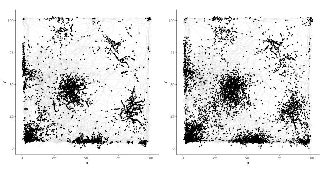
Figure 1: Left: True point pattern data (shown in black) on a trajectory $\Gamma_{\Omega}$ (shown in grey). Right: Simulated data on $\Gamma_{\Omega}$ from an inhomogeneous Poisson point process with estimated intensity function $\widehat{\lambda}_{\Gamma_{\Omega}}^{0}$ given by expression (1).

1.2 Current approaches for inferring grid cell activity

Current approaches for inferring the intensity of grid firing events rely mainly on kernel smoothing methods. Such methods are based on the firing rate map which is an estimator of the rate of occurrence of firing events per unit time at any spatial location (sargolini2006conjunctive). The estimator is defined by

$$\widehat{\lambda}_{\mathcal{T}}^{0}(s;h)=\int_{0}^{T}K_{h}\left(\lVert\Gamma_{\Omega}(t)-s\lVert\right)\,N_{\mathcal{T}}(\mathrm{d}t)\Big{/}\int_{0}^{T}K_{h}\left(\lVert\Gamma_{\Omega}(t)-s\lVert\right)\,\mathrm{d}t,~{}s\in\mathbb{R}^{2},T>0,h>0,$$ (1)

where $\Gamma_{\Omega}\,:\,[0,T]\rightarrow\mathrm{\mathbb{R}}^{2}$ denotes a continuously differentiable curve with $\Gamma_{\Omega}(t)=(s_{x}(t),s_{y}(t))$ representing the location of the animal in $\mathrm{\mathbb{R}}^{2}$ at time $t\in\mathcal{T}:=[0,T]$ and $N_{\mathcal{T}}$ denotes the counting process of firing events over time. The kernel function $K_{h}$ is defined by $K_{h}(s)=K(s/h)/h$, $s\in\mathrm{\mathbb{R}}^{2}$, where $K$ denotes the probability density of the bivariate Gaussian distribution with mean vector $(0,0)$ and variance-covariance matrix equal to the identity matrix $I_{2}\in\mathrm{\mathbb{R}}^{2\times 2}$. The parameter $h$ is a bandwidth parameter and $\lVert\,\cdot\,\lVert$ denotes the Euclidean norm. In what follows, time is measured in seconds, distances in centimeters and angles in radians.

To understand estimator (1), it is helpful to decompose it into the product of two estimators, one associated with the expected number of firing events per unit distance travelled at location $s$, and the other associated with the expected speed of the animal at location $s$. In particular, if we denote

$$W_{h}(t,s)=K_{h}(\lVert\Gamma_{\Omega}(t)-s\lVert)\Big{/}\int_{0}^{T}K_{h}(\lVert\Gamma_{\Omega}(t)-s\lVert)\,\mathrm{d}t\qquad\text{and}\qquad\dot{\Gamma}_{\Omega}(t)=\left(\frac{\mathrm{d}s_{x}(t)}{\mathrm{d}t},\frac{\mathrm{d}s_{y}(t)}{\mathrm{d}t}\right),$$

then we have that $\widehat{\lambda}_{\mathcal{T}}^{0}(s;h)=\widehat{\lambda}_{\Gamma_{\Omega}}^{0}(s;h)\,\widehat{v}(s;h)$, where rCl ^λ_$\Gamma_{\Omega}$^0(s; h) &= ∫_0^T K_h(∥$\Gamma_{\Omega}$(t) - s∥) N_$\mathcal{T}$($\mathrm{d}$t)/ ∫_$\Gamma_{\Omega}$ K_h(∥z-s ∥) $\mathrm{d}$z,
^v(s;h) = ∫_$\Gamma_{\Omega}$ K_h(∥z-s ∥) $\mathrm{d}$z / ∫_0^T K_h(∥$\Gamma_{\Omega}$(t)-s ∥) $\mathrm{d}$t = ∫_0^T W_h(t,s) ∥˙Γ_Ω(t)∥ $\mathrm{d}$t, with $\int_{\Gamma_{\Omega}}g(z)\,\mathrm{d}z$ denoting the line integral of an arbitrary integrable scalar field $g\,:\,\mathrm{\mathbb{R}}^{2}\rightarrow\mathrm{\mathbb{R}}$ along the curve $\Gamma_{\Omega}$. Thus, $\widehat{\lambda}_{\mathcal{T}}^{0}$ decomposes into the product of a kernel-smoothing based estimator $\widehat{\lambda}_{\Gamma_{\Omega}}^{0}$ for the intensity of a non-homogeneous Poisson point process on the trajectory $\Gamma_{\Omega}$ (diggle1985kernel) and a kernel-smoothing based estimator $\widehat{v}(s;h)$ of the expected speed of the animal at a given location $s$. This estimator is intrinsically non-parametric, but it assumes that for any interval of time $I\subseteq\mathcal{T}$ with $|I|>0$, the variation in the counts of firing events $N_{\mathcal{T}}(I)$ that are observed during $I$ is solely explained by how much area the animal explores and what regions it visits in this period of time.

Whilst seemingly simple, estimator (1) can be unwieldy. First, kernel smoothing methods may mask fine scale structure in the data and may produce overly smooth estimates. Although there are data-driven methods for choosing the bandwidth parameter, fixing it to $h=3\text{cm}$ (cf. sargolini2006conjunctive, supplementary material) appears to be common practice. Contrasting a realization of an inhomogeneous Poisson point process on $\Gamma_{\Omega}$, with intensity function equal to $\widehat{\lambda}_{\Gamma_{\Omega}}^{0}(,3)$ (Figure 1, right panel), with the ground-truth data (left panel), we see an effect of oversmoothing, e.g., in the bottom left region of the square arena. The ground-truth data exhibit an additional amount of clustering which is also not captured by the inhomogeneous Poisson point process. This questions the validity of the estimator and of the generic use of a fixed bandwidth parameter.

To the best of our knowledge, no systematic study on the smoothness properties of the firing activity of grid-cells exists. Although estimator (1) is continuously specified, it is typically computed by discretizing the spatial domain and then by using aggregated statistics such as counts of firing events. The counts are then used to estimate the firing activity.  Although this simplifies statistical modelling, it comes at a cost as it reduces estimation efficiency and may lead to ecological bias, whereby inferences obtained at the coarser scale are incorrectly carried over to the finer scale.

Second, the assumption that the variation in the number of counts $N_{\mathcal{T}}(I)$ is explained only by the animal’s locations in the period of time $I$ may not be sufficient. For example, the firing activity may also be explained by covariates other than the location of the animal such as the orientation of its head, which we will refer to as the head-direction. By discretizing the domain of the covariates and by computing counts within each part of the domain, gerlei2020grid gave evidence for an interaction effect between the location and the head-direction, with variations in the firing activity explained by combinations of locations and head-directions. Again, the concern of potential ecological bias due to discretization and aggregation effects also extends to the approach adopted by gerlei2020grid.

In this paper we are led to develop new statistical procedures for modelling the firing activity of grid cells that are flexible, extendible, and coherent at the finest possible scale. This requires a step-change in approach relative to current methodology and practice. In particular, we adopt a principled statistical approach based on log-Gaussian Cox processes. Our approach bypasses issues related to ecological bias as it avoids discretization and aggregation. Additionally, it allows inclusion of covariates in a straightforward manner. We build a range of statistical models which include biologically relevant covariates. We show better predictive performance from a model that includes an effect of interaction between the location and the head-direction of the animal, thereby confirming the results of gerlei2020grid. Our proposed statistical models are hierarchical and are built on the assumption that the intensity function is random, and its prior distribution is determined by that of a stationary Gaussian process. Owing to the strong oscillatory nature of the firing activity, we use Gaussian processes with underdamped Matérn covariance functions (lindetal11). The upshot of this choice is that our prior distributions mimic closely the effect of the covariates in the firing activity, and the fitting of the models can be performed efficiently due to the compactly supported basis function representation of our proposed Gaussian random fields. As a by-product, we give closed-form expressions for the marginal variance of Gaussian processes on $\mathrm{\mathbb{R}}$, $\mathrm{\mathbb{R}}^{2}$, and $\mathrm{\mathbb{S}_{1}}=[0,2\pi)$, with underdamped, critically damped, and overdamped Matérn covariances. We build our models in a Bayesian framework, which gives us a tool for fitting complex models, and the advantage of doing this efficiently with integrated nested Laplace approximation (INLA, rue2009approximate). We use the R package inlabru (inlabru), which is based on INLA and is specialized in dealing with structured data and has extensive support for point process models.

1.3 Paper structure

In Section 2 we describe the statistical framework that use throughout the paper. Preliminary notation associated with the experimental framework is presented Section 2.1. Section 2.2 introduces the class of log-Gaussian Cox processes and Section 2.3 describes a general framework for including covariates in the intensity function of a Poisson point process. Section 2.4 discusses the finite-dimensional Gaussian Markov random field (GMRF) approximations of the latent Gaussian random fields that we use to model the effect of covariates on the the firing rate of grid cells. In Section 2.5 we describe the properties of the continuous limit Gaussian random fields that the GMRFs presented in Section 2.4 converge to, and derive closed-form expressions for the variances, which are necessary for practical model fitting and the interpretation of the models. Section 3 details practical information about how we perform inference in practice. In particular, in Section 3.1 we present approximate closed-form expressions for the likelihood function and describe the numerical integration scheme that we use to evaluate the intractable integral associated with the void probability of each Poisson point process model. In Section LABEL:sec:prior, we complete the specification of the Bayesian models through choices of appropriate prior distributions for the hyperparameters. Section LABEL:sec:cs contains our implementation, analysis and interpretation of the proposed models through a case study example from the grid cell spike train shown in Figure 1. The data set is described in Section LABEL:sec:data. In Section LABEL:sec:cv, we assess the predictive performance of all models via cross-validation and in LABEL:sec:analysis we fit and interpret all models to the data. We conclude with a discussion that highlights the strengths of the methodology in Section LABEL:sec:discussion. Technical material and additional supporting evidence is presented in LABEL:sec:supplement (Supplementary Material).

2 Statistical modelling

2.1 Notation and framework

The standard experimental framework relates to an animal; typically a rodent moving in the interior of a bounded planar domain $\Omega\subset\mathbb{R}^{2}$; and is modelled by a filtered probability space $(E,\mathscr{H},\mathrm{\mathbf{P}},\mathscr{F})$ where $\mathscr{F}=(\mathscr{F}_{t})_{t\in\mathrm{\mathbb{R}}_{+}}$ denotes an increasing family of sub-$\sigma$-algebras of $\mathscr{H}$. The animal moves freely for a period of time $\mathcal{T}=[0,T]$, where $T:E\rightarrow\mathrm{\mathbb{R}}_{+}$ denotes a stopping time, i.e., $\{T\leq t\}\in\mathscr{F}_{t}$ for all $t>0$. The stopping time $T$ marks the end of the experiment and in practice, it is usually decided prior to the start of the experiment. Hence, we assume $T$ is non-informative. For any $t\in\mathcal{T}$, let the two-dimensional vector $\Gamma_{\Omega}(t)=(s_{x}(t),s_{y}(t))^{\top}\in\mathrm{\mathbb{R}}^{2}$ denote the spatial co-ordinates of the animal in $\Omega$ at time $t$, $\Gamma_{\Omega}(A)=\{\Gamma_{\Omega}(t)\,:\,t\in A\}$, $A\subseteq\mathcal{T}$, and $\Gamma_{\Omega}:=\Gamma_{\Omega}(\mathcal{T})$ for the continuously differentiable curve in $\Omega$ representing the entire trajectory of spatial locations of the animal throughout the duration of the experiment. Let $\{s_{0}:=\Gamma_{\Omega}(\tau_{0}),\ldots,s_{N}:=\Gamma_{\Omega}(\tau_{N})\}$ be a sample of locations taken from $\Gamma_{\Omega}$ at approximately regular times $\tau_{0},\tau_{1}\ldots,\tau_{N}\in\mathcal{T}$, i.e., $\tau_{i+1}-\tau_{i}\approx\Delta\tau>0$. Let also $\theta(t)\in\mathrm{\mathbb{S}_{1}}:=[0,2\pi)$ denote the head-direction of the animal at time $t$ and write $\{\theta_{0}:=\theta(\tau_{0}),\dots,\theta_{N}:=\theta(\tau_{N})\}$ for the sample of head-directions. Prior to time $\tau_{0}=0$, electrodes that measure the firing activity of a nerve cell are implanted in the brain of the animal. Let $f:E\rightarrow\{0,1\}^{\mathcal{T}}$ be a random variable from the sample space $E$ to the set of all functions on $\mathcal{T}$ with image $\{0,1\}$. For a fixed realization of the experiment the function $f$ encodes the activity of the neuron according to the convention: $f(t)=1$, if the neuron is active at time $t$ and $f(t)=0$, otherwise. In what follows, it is assumed that available are the labeled data $\{(s_{1},\theta_{1},f(\tau_{1})),\ldots,(s_{N},\theta_{N},f(\tau_{N}))\}$. We write $t_{1},\dots,t_{n}$ for the set of times the neuron is active, that is, $\{t_{i}\,:\,i=1,\dots,n\}=\{\tau_{j}\,:\,f(\tau_{j})=1\}$.

2.2 Cox processes

Let $N_{\mathcal{T}}\,:\,E\times\mathscr{H}\rightarrow(\mathrm{\mathbb{R}}_{+},\mathscr{B}(\mathrm{\mathbb{R}}_{+}))$ be a random counting measure on $(\mathrm{\mathbb{R}}_{+},\mathscr{B}(\mathrm{\mathbb{R}}_{+}))$, that is, $e\mapsto N_{\mathcal{T}}(e,A)$ is a random variable for each $A\in\mathscr{B}(\mathrm{\mathbb{R}}_{+})$ and $A\mapsto N_{\mathcal{T}}(e,A)$ is, for almost every $e\in E$, a purely atomic measure and its every atom has weight one. We shall denote by $N_{\mathcal{T}}(A)$ the former random variable and we will associate with it the number of firing events in a Borel subset $A$ of time. Let also $\Lambda_{\mathcal{T}}\,:\,E\times\mathscr{H}\rightarrow(\mathrm{\mathbb{R}}_{+},\mathscr{B}(\mathrm{\mathbb{R}}_{+}))$ be a random measure on $(\mathrm{\mathbb{R}}_{+},\mathscr{B}(\mathrm{\mathbb{R}}_{+}))$ satisfying, $\Lambda_{\mathcal{T}}(A)=\int_{A}\lambda_{\mathcal{T}}(t)\,\mathrm{d}t$ for any $A\in\mathscr{B}(\mathrm{\mathbb{R}}_{+})$, where $\lambda_{\mathcal{T}}=(\lambda_{\mathcal{T}}(t))_{t\in\mathrm{\mathbb{R}}_{+}}$ is a positive continuous stochastic process. In what follows, we say that the counting process $N_{\mathcal{T}}$ follows a Cox process with random intensity $\lambda_{\mathcal{T}}$ if the conditional expectation of $\exp(-N_{\mathcal{T}}f)$ given the sigma-algebra $\mathscr{F}$ generated by $\Lambda_{\mathcal{T}}$ is

$$\mathbb{E}\left\{\exp(-N_{\mathcal{T}}f)\mid{\mathscr{F}}\right\}=\exp\left(-\int_{\mathrm{\mathbb{R}}_{+}}[1-\exp\{-f(t)\}]\,\lambda_{\mathcal{T}}(t)\,\mathrm{d}t\right),\qquad f\in\mathscr{B}(\mathrm{\mathbb{R}}_{+}),\quad f\geq 0,$$

that is, conditionally on the intensity function $\lambda_{\mathcal{T}}$, the process $N_{\mathcal{T}}$ is an inhomogeneous Poisson point process with intensity $\lambda_{\mathcal{T}}$ on $\mathcal{T}$, meaning that for any countable collection of disjoint subsets $A_{1},\ldots,A_{k}\subseteq\mathscr{B}(\mathrm{\mathbb{R}}_{+})$, we have l N_$\mathcal{T}$(A_i)∣$\lambda_{\mathcal{T}}$∼Poisson(∫_A_i $\lambda_{\mathcal{T}}$(t) $\mathrm{d}$t)  and  $N_{\mathcal{T}}(A_{1}),\ldots,N_{\mathcal{T}}(A_{k})$ are independent given $\lambda_{\mathcal{T}}$. Cox processes have been applied in various fields such as ecology, epidemiology, neuroscience, and image analysis. This is because Cox processes can model point patterns that exhibit both clustering and inhomogeneity, which is a trait observed in many natural phenomena. Another reason for the widespread use of Cox processes is their flexibility and capacity for statistical modelling. The requirements that are needed on the properties of $\lambda_{\mathcal{T}}$ so that $N_{\mathcal{T}}$ exists are minimal and this accommodates a broad class of models for the random intensity function $\lambda_{\mathcal{T}}$. Amongst the most popular ones, the log-Gaussian Cox process (LGCP) models the logarithm of the random intensity of the point process $N_{\mathcal{T}}$ as a Gaussian process, which allows for flexible modelling of the variability of the point pattern, and can model the effect of covariates in a non-linear manner. LGCPs are also useful for Bayesian inference, as the Gaussian process prior facilitates efficient numerical algorithms.

Given the $\sigma$-field $\mathscr{F}$ generated by $\Lambda_{\mathcal{T}}$ and a point pattern $\{t_{1},\ldots,t_{n}\}$ in a bounded set $\mathcal{T}\subset\mathrm{\mathbb{R}}_{+}$, the likelihood of an inhomogeneous Poisson process is

$$L(\lambda_{\mathcal{T}})=\exp\left[\int_{\mathcal{T}}\{1-\lambda_{\mathcal{T}}(t)\}\,\mathrm{d}t\right]\,\prod_{i=1}^{n}\lambda_{\mathcal{T}}(t_{i}).$$ (2)

Because likelihoods are needed up to a proportionality factor, expression (2) is often presented without the term “1” that appears in the exponent in the first factor. Such a simplification in the likelihood function (2) is valid provided the domain of the point process remains unchanged. However, when one is interested in modelling and inferring the distribution of $N_{\mathcal{T}}$ subject to changes in its domain, then (2) cannot be simplified further.

2.3 Statistical models for spike trains from grid cells

To facilitate generality, we define the configuration space of the system to be the set of allowable positions relative to a reference state. For example, consider an animal whose body is moving in a two dimensional Euclidean space and whose orientation in space is changing according to a direction in the unit circle. Then we may take the configuration space to be the Riemannian manifold $\mathrm{\mathbb{R}}^{2}\times\mathbb{S}_{1}$. More generally, we can label the configuration of the animal by a system of generalized coordinates $x=(x_{1},\dots,x_{m})$, where $x_{j}\in\mathcal{X}_{j}\subseteq\mathrm{\mathbb{R}}^{d_{j}},j=1,\ldots,m$, $d_{j},m\in\mathbb{N}$, so that for the aforementioned example, we have $x_{1}=(s_{x},s_{y})$ and $x_{2}=\theta$ with $(s_{x},s_{y})$ denoting the row vector of Cartesian coordinates in $\mathcal{X}_{1}=\mathrm{\mathbb{R}}^{2}$ and $\theta$ denoting an angle in $\mathcal{X}_{2}=\mathbb{S}_{1}=[0,2\pi)$. In the course of an experiment, the animal undergoes dynamical evolution so it continuously changes its position. This evolution can be specified by giving the generalized coordinate location of the animal as a function of time, that is, $(x_{1},\dots,x_{m})=(x_{1}(t),\dots,x_{m}(t))$ for $t\in\mathcal{T}$. This defines a curve of covariates $\Gamma=\{\Gamma(t)\,:\,t\in\mathcal{T}\}$ where $\Gamma(t)=(x_{1}(t),\dots,x_{m}(t))$ which we assume to be continuously differentiable. It is worth to remark here that prior to the start of the experiment, $\Gamma$ is unknown. Hence, $\Gamma$ may be taken to be a random element, that is, a map that is measurable relative to $\mathscr{H}$ and $\mathscr{B}(\mathcal{X})$, where $\mathcal{X}:=\prod_{j=1}^{m}\mathcal{X}_{j}$. In a Bayesian setting, this assumption is equivalent to treating $\Gamma$ as a statistical parameter in a hierarchical statistical model. Such an approach would allow inference to be made about the dynamics of the trajectory of the animal and potentially, about its effects on the intensity of the point pattern, via the assignment of a prior distribution on $\Gamma$ and via posterior updating of prior beliefs. However, owing to the fact that there is no evidence for an effect from the dynamics of $\Gamma$ on the firing properties of grid-cells, which is the main application and emphasis of this paper, we shall henceforth treat the trajectory as known and fixed a priori, and we will construct statistical models conditionally on the curve $\Gamma$.

To model the effect of the covariates on the number of spikes per unit time at time $t$, we need to link the random mean measure $\Lambda_{\mathcal{T}}$ to a random measure on $\mathcal{X}$. This is accomplished by specifying $\Lambda_{\mathcal{T}}$ in terms of a mapping $l$ that is measurable relative to the join sigma-algebra $\mathscr{B}(\mathcal{X})\vee\mathscr{B}(\mathcal{T})$ and the sigma-algebra $\mathscr{B}(\mathrm{\mathbb{R}}_{+})$, that is, $\Lambda_{\mathcal{T}}(\mathrm{d}t)=l(\mathrm{d}\Gamma(t),\mathrm{d}t)$. To define the distance near each point of the smooth manifold $\mathcal{X}$, we endow $\mathcal{X}$ with a Riemannian metric that specifies infinitesimal distances on $\mathcal{X}$. A Riemannian metric assigns to each $x$ a positive-definite inner product $g_{x}\,:\,T_{x}\,\mathcal{X}\times T_{x}\,\mathcal{X}\rightarrow\mathrm{\mathbb{R}}$ where $T_{x}\mathcal{X}$ is the tangent space at $x$. Given a system of generalized coordinates $x\,:\,U\rightarrow\mathrm{\mathbb{R}}^{\sum_{j}d_{j}}$ on an open set $U$ of $\mathcal{X}$, the vectors $(\partial/\partial x_{1}\mid_{x},\dots,\partial/\partial x_{m}\mid_{x})$ form a basis of the vector space $T_{x}\mathcal{X}$ for any $x\in U$. Relative to this basis, we define the metric components of a metric tensor $G=(g_{ij\mid x})_{1\leq i,j\leq m}$ at each $x$ by $g_{ij\mid x}=g_{x}(\partial/\partial x_{i}\mid_{x},\partial/\partial x_{j}\mid_{x})$. With this notation, our general modelling framework presupposes that the expected number of spikes per unit time at time $t$ equals to the expected number of spikes per unit generalized travel distance at generalized coordinate $x(t)$, multiplied by the generalized speed of the particle at time $t$. This is compactly written as

$$\Lambda_{\mathcal{T}}(\mathrm{d}t)=\lambda_{\mathcal{T}}(t)\,\mathrm{d}t=\lVert\dot{x}(t)\rVert\,\lambda_{\mathcal{X}}(x(t)),$$ (3)

where $\lVert\dot{x}(t)\rVert^{2}=\{(\mathrm{d}x(t)/\mathrm{d}t)^{\top}\,G\,(\mathrm{d}x(t)/\mathrm{d}t)\}$ and $\lVert\dot{x}(t)\rVert$ is the local derivative of the geodesic metric induced by the Riemannian metric $G$ along the curve $\Gamma$ (adler2007random). Here $\log\lambda_{\mathcal{X}}$ is a real-valued stochastic process on $\mathcal{X}$.

A natural choice for the metric tensor $G$ in our setting is $G=\text{diag}(1,1,\delta)$ where $\delta$ is measured in meters per radians, that is, the metric tensor only involves an axis aligned scaling in the direction of $\theta$, which gives $\rVert\dot{x}(t)\lVert^{2}=\dot{s_{x}}(t)^{2}+\dot{s_{y}}(t)^{2}+\delta\,\dot{\theta}(t)^{2}$. The parameter $\delta$ is an unknown parameter and in our implementations, we selected a prior distribution degenerate at $0$, which implies that firing events cannot occur due changes in the head-direction of the animal whilst the animal stays still; this choice was motivated by subject expert knowledge and for the simplicity it affords. Thus, in our implementation we use $\lVert\dot{x}(t)\rVert=\lVert\dot{\Gamma}_{\Omega}(t)\rVert$ which is the speed of the animal. However, it is worth to remark that, should there be need for the use of a different prior for $\delta$, then this parameter could be inferred even if instances in the data where the animal stays still have been filtered out.

Based on these choices, in this paper we consider the models rCl $\mathcal{M}_{\Omega}$:  $\Lambda_{\mathcal{T}}$(dt)&=Λ_Ω ($\Gamma_{\Omega}$($\mathrm{d}$t)) := ∥$\dot{\Gamma}_{\Omega}$(t)∥ λ_Ω ($\Gamma_{\Omega}$(t)),
$\mathcal{M}_{\Omega,\mathcal{T}}$:  $\Lambda_{\mathcal{T}}$(dt)=Λ_Ω,$\mathcal{T}$ ($\Gamma_{\Omega}$($\mathrm{d}$t),$\mathrm{d}$t) := ∥$\dot{\Gamma}_{\Omega}$(t)∥ λ_Ω ($\Gamma_{\Omega}$(t)) h_$\mathcal{T}$(t),
$\mathcal{M}_{\Omega\times\Theta}$:  $\Lambda_{\mathcal{T}}$(dt)=Λ_Ω×Θ ($\Gamma_{\Omega}$($\mathrm{d}$t), θ($\mathrm{d}$t)) := ∥$\dot{\Gamma}_{\Omega}$(t)∥  λ_Ω×Θ ($\Gamma_{\Omega}$(t), θ(t)),
$\mathcal{M}_{\Omega\times\Theta,\mathcal{T}}$:  $\Lambda_{\mathcal{T}}$(dt)=Λ_Ω×Θ, $\mathcal{T}$ ( $\Gamma_{\Omega}$($\mathrm{d}$t),θ($\mathrm{d}$t), $\mathrm{d}$t)  := ∥$\dot{\Gamma}_{\Omega}$(t) ∥  λ_Ω×Θ ($\Gamma_{\Omega}$(t), θ(t)) h_$\mathcal{T}$(t), where $\lambda_{\Omega}$, $\lambda_{\Omega\times\Theta}$ and $h_{\mathcal{T}}$ denote positive continuous stochastic process on $\Omega$, $\Omega\times\Theta$ and $\mathcal{T}$, respectively, and are described in detail in Sections 2.4 and 2.5.

Model $\mathcal{M}_{\Omega}$ assumes that the variation in the number of spikes is solely explained by how much area the animal explores and what regions it visits in a period of time. In particular, in $\mathcal{M}_{\Omega}$, the expected number of spikes per unit time at time $t$ is the product of the expected number of spikes per travel distance at location $\Gamma_{\Omega}(t)$, which is measured by $\lambda_{\Omega}(\Gamma_{\Omega}(t))$, with the speed of the animal at time $t$, which is measured by $\lVert\dot{\Gamma}_{\Omega}(t)\rVert$. Hence, $\mathcal{M}_{\Omega}$ is similar in spirit with the model formulation and estimator (1) of sargolini2006conjunctive that we presented in Section 1.2, and hence, it will serve as our baseline model. Model $\mathcal{M}_{\Omega\times\Theta}$ assumes that the variation in the number of spikes is explained by how much area the animal explores and what regions in $\mathrm{\mathbb{R}}\times\mathrm{\mathbb{S}_{1}}$ it visits in a period of time. Specifically, in $\mathcal{M}_{\Omega,\mathcal{T}}$, the expected number of spikes per unit time at time $t$ is the product of the expected number of spikes per travel distance at the generalized coordinate $(\Gamma_{\Omega}(t)^{\top},\theta(t))$, which is measured by $\lambda_{\Omega\times\Theta}(\Gamma_{\Omega}(t),\theta(t))$, with the speed of the animal at time $t$.

Models $\mathcal{M}_{\Omega,\mathcal{T}}$ and $\mathcal{M}_{\Omega\times\Theta,\mathcal{T}}$ include an additional factor $h_{\mathcal{T}}$ which modulates the firing rate as a function of experimental clock time, see for example kassvent01 for a similar construction. Here, the stochastic process $h_{\mathcal{T}}$ is dimensionless and hence, the interpretation of $\lambda_{\Omega}$ and $\lambda_{\Omega\times\Theta}$ is identical to that in models $\mathcal{M}_{\Omega}$ and $\mathcal{M}_{\Omega\times\Theta}$, respectively. The rationale for including a modulating factor in models $\mathcal{M}_{\Omega,\mathcal{T}}$ and $\mathcal{M}_{\Omega\times\Theta,\mathcal{T}}$ stems from the likely scenario of additional, unobserved covariates, explaining variation in the number and properties of firing events which is not explained by $\lambda_{\Omega}$ or $\lambda_{\Omega\times\Theta}$ alone.

2.4 Continuously specified finite-dimensional Gaussian random fields

Inference can be facilitated through specification of the law of the stochastic process $\lambda_{\mathcal{X}}$. The most common and practically useful choice is that of $\lambda_{\mathcal{X}}$ being a log-Gaussian process, i.e., a random field on $\mathcal{X}$ for which the finite-dimensional distributions of $(\log\lambda_{\mathcal{X}}(x_{1}),\ldots,\log\lambda_{\mathcal{X}}(x_{m}))$ are multivariate Gaussian for each $1\leq m\leq\infty$ and each $(x_{1},\ldots,x_{m})\in\mathcal{X}$.

The firing rate per unit displacement per unit generalized distance at generalized coordinate $x\in\mathcal{X}$, and the modulating factor are modelled as $\log\lambda_{\mathcal{X}}(x)=\beta+\xi_{\mathcal{X}}(x)$ and $\log h_{\mathcal{T}}(t)=\xi_{\mathcal{T}}(t),$ where $\beta$ denotes a background constant firing rate and $\xi_{\mathcal{X}}$ and $\xi_{\mathcal{T}}$ are stationary zero-mean Gaussian processes on $\mathcal{X}$ and $\mathcal{T}$, respectively. Specifying a joint covariance structure over $\mathcal{X}=\mathcal{X}_{1}\times\cdots\times\mathcal{X}_{m}$ is highly demanding and it is natural to simplify this task by treating the joint covariance as separable in the input of the random field $\xi_{\mathcal{X}}$, i.e., to assume the covariance function has a Kronecker product form (see roug08) which asserts that $\mbox{$\text{cov}$}(\xi(x),\xi(x^{\prime}))=\prod_{i=1}^{m}\zeta_{i}(x_{i},x^{\prime}_{i}),x,x^{\prime}\in\mathcal{X},$, where $\zeta_{i}\,:\,\mathcal{X}_{i}\rightarrow\mathrm{\mathbb{R}}$ is a valid covariance function, i.e., a non-negative definite function on $\mathcal{X}_{i}$.

For the differentiable manifolds $\mathcal{X}_{1}:=\Omega\subset\mathrm{\mathbb{R}}^{2}$ and $\mathcal{X}_{2}:=\Theta:=[0,2\pi)$, we specify the latent random fields using the finite dimensional models $\xi_{\Omega}(s)=\bm{\psi}^{\Omega}(s)^{\top}\bm{w}^{\Omega}$, $\xi_{\Theta}(\theta)=\bm{\psi}^{\Theta}(\theta)^{\top}\bm{w}^{\Theta}$, $\xi_{\Omega\times\Theta}(s,\theta)=\bm{\psi}^{\Theta}(\theta)^{\top}\bm{w}^{\Omega\times\Theta}\bm{\psi}^{\Omega}(s)$ and $\xi_{\mathcal{T}}(t)=\bm{\psi}^{\mathcal{T}}(t)^{\top}\bm{w}^{\mathcal{T}}$, where $\bm{w}^{\Omega}_{p_{\Omega}\times 1}\sim\mathsf{N}(\bm{0},\bm{Q}_{\Omega}(\bm{\chi}_{\Omega})^{-1})$, $\bm{w}^{\Theta}_{p_{\Theta}\times 1}\sim\mathsf{N}(\bm{0},\bm{Q}_{\Theta}(\bm{\chi}_{\Theta})^{-1})$, $\text{vec}((\bm{w}_{p_{\Theta}\times p_{\Omega}}^{\Omega\times\Theta})^{\top})_{(p_{\Omega}\,p_{\Theta})\times 1}\sim\mathsf{N}(\bm{0},\bm{Q}_{\Omega}(\bm{\chi}_{\Omega})^{-1}\otimes\bm{Q}_{\Theta}(\bm{\chi}_{\Theta})^{-1})$, and $\bm{w}^{\mathcal{T}}_{p_{\mathcal{T}}\times 1}\sim\mathsf{N}(\bm{0},\bm{Q}_{\mathcal{T}}(\bm{\chi}_{\mathcal{T}})^{-1})$, are independent vectors of stochastic weights; $\bm{\psi}^{\Omega}=(\psi_{i}^{\Omega}\,:\,i=1,\dots,p_{\Omega})$, $\bm{\psi}^{\Theta}=(\psi_{j}^{\Theta}\,:\,i=1,\dots,p_{\Theta})$, and $\bm{\psi}^{\mathcal{T}}=(\psi_{k}^{\mathcal{T}}\,:\,i=1,\dots,p_{\mathcal{T}})$, are deterministic piecewise linear basis functions on $\mathrm{\mathbb{R}}^{2},\Theta$ and $\mathrm{\mathbb{R}}$, defined for each node on a spatial, circular, and temporal mesh, respectively; vec and $\otimes$ denote vectorization of a matrix by stacking its column vectors on top of one another and Kronecker product, respectively; and $\bm{Q}_{\Omega}(\bm{\chi}_{\Omega})$, $\bm{Q}_{\Theta}(\bm{\chi}_{\Theta})$ and $\bm{Q}_{\Omega}(\bm{\chi}_{\Omega})$ are positive-definite precision matrices defined by $\bm{Q}_{\cdot}(\bm{\chi}_{\cdot})=\tau_{\cdot}^{2}(\kappa_{\cdot}^{4}C_{\cdot}+2\varphi_{\cdot}\kappa_{\cdot}^{2}G_{\cdot}+G_{\cdot}C_{\cdot}^{-1}G_{\cdot})$, where $\bm{\chi}_{\cdot}=(\kappa_{\cdot},\tau_{\cdot},\varphi_{\cdot})$, $\kappa_{\cdot},\tau_{\cdot}>0$, $\varphi_{\cdot}\in(-1,\infty)$, $C_{\cdot}=(C_{rc}^{\cdot})_{r,c=1}^{p_{\cdot}}$ with $C_{rc}^{\cdot}=\langle\psi_{r}^{\cdot},\psi_{c}^{\cdot}\rangle$, and $G_{\cdot}=(G_{rc}^{\cdot})_{r,c=1}^{p_{\cdot}}$ with $G_{rc}^{\cdot}=\langle\nabla\psi_{r}^{\cdot},\nabla\psi_{c}^{\cdot}\rangle$. Here, $\cdot$ is used as a placeholder for $\Omega,\Theta$ and $\mathcal{T}$ and $\langle\psi_{r}^{\cdot},\psi_{c}^{\cdot}\rangle:=\int_{\cdot}\psi_{r}^{\cdot}(e)\psi_{c}^{\cdot}(e)\lambda_{\cdot}(e)$, where $\lambda_{\cdot}$ denotes the Lebesgue measure on the respective domain.

The vectors of stochastic weights belong to the class of Gaussian Markov random fields (GMRF) (rueheld05) and their Markovian properties are determined by the graph structure of the mesh. The weights control the stochastic properties of $\xi_{\Omega},\xi_{\Theta},\xi_{\Omega\times\Theta}$ and $\xi_{\mathcal{T}}$, and are chosen so that the distibution of each linear combination converges to the distribution of the solution of an SPDE, see simpsetal16 for more details.

2.5 Limiting infinite-dimensional Gaussian random fields

When the parameters $\varphi_{\Omega}$ and $\varphi_{\Theta}$ are equal to unity, then all random fields presented in Section 2.4 converge strongly (lindetal11; simpsetal16) to Gaussian random fields with Matérn covariance functions, a class of random fields that is widely adopted in spatial statistics (stein1999interpolation). In particular, the models that we presented in the previous section are Hilbert space projections of solutions of the Whittle–Matérn stochastic (partial) differential equation (lindetal11; lindgren2022spde). The continuously specified infinite-dimensional limits of the Gaussian random fields $\xi_{\Omega}$, $\xi_{\Theta}$ and $\xi_{\mathcal{T}}$ are Gaussian random fields with power spectral mass/density functions rCl f_Ω(ω) &= σΩ2(2π)2(1 κΩ4+ 2  φΩκΩ2∥ω∥2+ ∥ω∥4)^α_Ω/2,   ω∈$\mathrm{\mathbb{R}}$^2
f_Θ(ω)= σΘ22π (1κΘ4+2φΘκΘ2ω2+ ω4)^α_Θ/2,   ω∈$\mathbb{Z}$
f_$\mathcal{T}$(ω) = σ$\mathcal{T}$22π (1κ$\mathcal{T}$4+2φ$\mathcal{T}$κ$\mathcal{T}$2ω2+ω4)^α_$\mathcal{T}$/2,  ω∈$\mathrm{\mathbb{R}}$. respectively, where the shape parameters satisfy $\alpha_{\Omega}=\alpha_{\Theta}=\alpha_{\mathcal{T}}=2$. We work with the special case where all shape parameters are equal to 2, for the simplicity and clarity this choice affords. The covariance functions may be given in analytic form for some cases only, e.g., on $\mathrm{\mathbb{R}}$ and $\mathrm{\mathbb{R}}^{2}$, inversion of the spectrum gives (lindetal11) rClr ζ_Ω(s) &= σΩ24 πsin(πγΩ) κΩ2i [K_0{κ_Ω∥s ∥exp(-i πγΩ2)} -K_0{κ_Ω∥s ∥exp(i πγΩ2)}],
ζ_$\mathcal{T}$(t) = σ$\mathcal{T}$22 sin(πγ$\mathcal{T}$) κ$\mathcal{T}$3 exp{-κ_$\mathcal{T}$cos(πγ$\mathcal{T}$2 |t|)} sin{πγ$\mathcal{T}$2 + κ_$\mathcal{T}$sin(πγ$\mathcal{T}$2|t|)},   where $\varphi_{\Omega},\varphi_{\mathcal{T}}\in(-1,1]$ and $\gamma_{\cdot}=\text{arccos}(\varphi_{\cdot})/\pi$. On $\mathrm{\mathbb{S}_{1}}$ the covariance is obtained in analytic form only for the case $\varphi_{\Theta}=1$ and is given in Proposition 1 below.

Figure 2: Realizations of a zero-mean Gaussian random field $\xi_{\Omega}(s)$ with spectral density (2.5), where $\alpha_{\Omega}=2$, $\kappa_{\Omega}=0.2$ and $s_{\Omega}^{2}=1$. Top, left to right: shown for $\varphi_{\Omega}=-9.99/10,-9.9/10,-9/10,-2/10$. Bottom, right to left: shown for $\varphi_{\Omega}=2/10,9/10,9.9/10,9.99/10$.

Proposition 1.

A stationary Gaussian process $\xi_{\Theta}(\theta)$, $\theta\in\mathrm{\mathbb{S}_{1}}$, with power spectrum (2.5) with $\varphi_{\Theta}=1$, has covariance function rCl ζ_Θ(θ) &= σΘ24 sinh2(πκΘ) κΘ2{|θ|2 cosh{(2π-|θ|)κ_Θ}+

    + (π- |θ|2) cosh(|θ| κ_Θ) + κ_Θ^-1 [cosh{(π-|θ|)κ_Θ)  sinh(πκ_Θ}]}.

A proof is given in Section LABEL:app:covariance_circular of the supplement. Although the covariance is available in closed-form only under special cases, this is not a substantial inconvenience, as what is needed for practical model fitting are the discretised precision matrices from Section 2.4, and for convenience, e.g. for normalisation and parameter interpretation, the marginal variance. The marginal variances for the processes on $\mathrm{\mathbb{R}}^{2}$, $\mathrm{\mathbb{S}_{1}}$ and $\mathrm{\mathbb{R}}$ are given in Propositions 2, 3 and 4.

Figure 3: Realizations of $\xi_{\Theta}(\theta)-\xi_{\Theta}(0)$ where $\xi_{\Theta}$ is a zero-mean Gaussian random field with spectral mass function (2.5), where $\alpha_{\mathcal{T}}=2$, $\kappa_{\Theta}=2\pi$ and $s_{\Theta}^{2}=1$. Realizations are plotted in polar coordinates, with scale units marked by circles (center refers to scale value $-5$ and outer circle refers to scale value $5$). The circle shown in dark grey refers to the scale value $0$. Top, left to right: shown for $\varphi_{\Theta}=-9.99/10,-9.9/10,-9/10,-2/10$. Bottom, right to left: shown for $\varphi_{\Theta}=2/10,9/10,9.9/10,9.99/10$.

Proposition 2.

A stationary Gaussian process $\xi_{\Omega}(s)$, $s\in\mathrm{\mathbb{R}}^{2}$, with power spectrum (2.5) has marginal variance $s_{\Omega}^{2}:=\text{var}\{\xi_{\Omega}(s)\}$ given by

$$s_{\Omega}^{2}=\begin{dcases}\frac{\sigma_{\Omega}^{2}}{4\pi\kappa_{\Omega}^{2}\sqrt{1-\varphi_{\Omega}^{2}}}\arccos\varphi_{\Omega},&\text{underdamped},\varphi_{\Omega}\in(-1,1),\\ \frac{\sigma_{\Omega}^{2}}{4\pi\kappa_{\Omega}^{2}},&\text{critically damped},\varphi_{\Omega}=1,\\ \frac{\sigma_{\Omega}^{2}}{4\pi\kappa_{\Omega}^{2}\sqrt{\varphi_{\Omega}^{2}-1}}\left\{\frac{\pi}{2}-\text{atan}\left(\frac{\varphi_{\Omega}}{\sqrt{\varphi_{\Omega}^{2}-1}}\right)\right\},&\text{overdamped},\varphi_{\Omega}\in(1,\infty).\end{dcases}$$

Proposition 3.

A stationary Gaussian process $\xi_{\Theta}(\theta)$, $\theta\in\mathrm{\mathbb{S}_{1}}$, with power spectrum (2.5) has marginal variance $s_{\Theta}^{2}:=\text{var}\{\xi_{\Theta}(\theta)\}$ given by

$$s_{\Theta}^{2}=\begin{dcases}\frac{\sigma_{\Theta}^{2}}{4\kappa_{\Theta}^{3}\sqrt{1-\phi_{\Theta}^{2}}}\frac{2\{y\sin(2\pi\kappa_{\Theta}x)+x\sinh(2\pi\kappa_{\Theta}y)\}}{\left\{\cos(2\pi\kappa_{\Theta}x)-\cosh(2\pi\kappa_{\Theta}y)\right\}}&\text{underdamped},\varphi_{\Theta}\in(-1,1)\\ \frac{\sigma_{\Theta}^{2}}{4\kappa_{\Theta}^{3}}&\text{critically damped},\varphi_{\Theta}=1\\ \frac{\sigma_{\Theta}^{2}}{4\kappa_{\Theta}^{3}\sqrt{\varphi_{\Theta}^{2}-1}}\left(\frac{\cot\left(iz\right)}{iz}-\frac{\cot\left(i\overline{z}\right)}{i\overline{z}}\right),\quad&\text{overdamped},\varphi_{\Theta}\in(1,\infty)\end{dcases}$$

where $x=\cos(\gamma/2)$, $y=\sin(\gamma/2)$ and $\gamma\in[-\pi,0)$ satisfies $\exp(\iota\gamma)=-\phi_{\Theta}-\sqrt{1-\phi_{\Theta}^{2}}$.

Figure 4: Realizations of $\xi_{\mathcal{T}}(t)$ where $\xi_{\mathcal{T}}$ is a zero-mean Gaussian random field with spectral density (2.5), where $\alpha_{\mathcal{T}}=2$, $\kappa_{\mathcal{T}}=2/10$ and $s_{\mathcal{T}}^{2}=1$. Top, left to right: shown for $\varphi_{\mathcal{T}}=-9/10,-7/10,-4/10,-1/10$. Bottom, right to left: shown for $\varphi_{\mathcal{T}}=1/10,4/10,7/10,9/10$.

Proposition 4.

A stationary Gaussian process $\xi_{\mathcal{T}}(t)$, $t\in\mathrm{\mathbb{R}}_{+}$, with power spectrum (2.5) has marginal variance $s_{\mathcal{T}}^{2}:=\text{var}\{\xi_{\mathcal{T}}(t)\}$ given by

$$s_{\mathcal{T}}^{2}=\frac{\sigma_{\mathcal{T}}^{2}}{4\kappa_{\mathcal{T}}^{3}}\left(\frac{2}{1+\varphi_{\mathcal{T}}}\right)^{1/2},\qquad\varphi_{\mathcal{T}}>-1,$$

and is underdamped for $\varphi_{\mathcal{T}}\in(-1,1)$, critically damped for $\varphi_{\mathcal{T}}=1$, and overdamped for $\varphi_{\mathcal{T}}>1$.

Proofs of Propositions 2 3 and 4 are given in Section LABEL:sec:variances of the supplement.

3 Practical computation and parameter construction

3.1 Numerical evaluation of log-likelihood functions

The logarithm of the likelihood function (2) consists of two terms: a stochastic integral and the evaluation of the random field at the data points. Hence, the log-likelihood is analytically intractable as it requires the integral of the intensity function which cannot be calculated explicitly. The integral can, however, be approximated numerically using the approach of simpsetal16 who introduced a computationally efficient method for performing inference on log-Gaussian Cox processes based on continuously specified finite-dimensional Gaussian random fields. The remainder of this section describes the integration schemes that we use for the integrals in the log-likelihood functions of models $\mathcal{M}_{\Omega}$, $\mathcal{M}_{\Omega,\mathcal{T}}$, $\mathcal{M}_{\Omega\times\Theta}$, and $\mathcal{M}_{\Omega\times\Theta,\mathcal{T}}$, that is, the integration scheme that is used for the integrals rCl I_Ω &= -e^β∑_i=1^N ∫_t_i-1^t_iexp[ ψ^Ω{s(t)}^⊤  w^Ω] $\Gamma_{\Omega}$($\mathrm{d}$t),
I_Ω,$\mathcal{T}$ = -e^β∑_i=1^N ∫_t_i-1^t_iexp[ ψ^Ω{s(t)}^⊤  w^Ω + ψ^$\mathcal{T}$(t)^⊤w^$\mathcal{T}$] $\Gamma_{\Omega}$($\mathrm{d}$t),
I_Ω×Θ = -e^β∑_i=1^N∫_0^Texp[ψ^Ω×Θ{s(t), θ(t)}^⊤  w^Ω×Θ]$\Gamma_{\Omega}$($\mathrm{d}$t),  and
 I_Ω×Θ,$\mathcal{T}$ = -e^β∑