Hierarchical Fine-Grained Image Forgery Detection and Localization

Abstract

Differences in forgery attributes of images generated in CNN-synthesized and image-editing domains are large, and such differences make a unified image forgery detection and localization (IFDL) challenging. To this end, we present a hierarchical fine-grained formulation for IFDL representation learning. Specifically, we first represent forgery attributes of a manipulated image with multiple labels at different levels. Then we perform fine-grained classification at these levels using the hierarchical dependency between them. As a result, the algorithm is encouraged to learn both comprehensive features and inherent hierarchical nature of different forgery attributes, thereby improving the IFDL representation. Our proposed IFDL framework contains three components: multi-branch feature extractor, localization and classification modules. Each branch of the feature extractor learns to classify forgery attributes at one level, while localization and classification modules segment the pixel-level forgery region and detect image-level forgery, respectively. Lastly, we construct a hierarchical fine-grained dataset to facilitate our study. We demonstrate the effectiveness of our method on $7$ different benchmarks, for both tasks of IFDL and forgery attribute classification. Our source code and dataset can be found: github.com/CHELSEA234/HiFi-IFDL.

1 Introduction

\begin{overpic}[width=248.42812pt]{figure/manipulation_area_distribution.pdf} \par\put(57.5,69.0){\small{Detection}} \put(54.0,50.5){\small{Localization}} \put(73.0,66.5){\small{{\color[rgb]{1,0,0}Real} {v.s.} Forgery}} \put(15.0,61.5){\small{Image Editing}} \put(12.0,46.5){\small{CNN-synthesized}} \put(49.0,41.0){(a)} \par\put(0.0,1.0){\rotatebox{90.0}{{\scriptsize{Mean/Variance of forgery area}}}} \put(3.5,33.0){\footnotesize{$.5$}} \put(3.5,26.5){\footnotesize{$.4$}} \put(3.5,20.0){\footnotesize{$.3$}} \put(3.5,13.5){\footnotesize{$.2$}} \put(3.5,7.5){\footnotesize{$.1$}} \put(49.0,-1.5){(b)} \par\par\end{overpic}

Figure 1: (a) In this work, we study image forgery detection and localization (IFDL), regardless of forgery method domains. (b) The distribution of forgery region depends on individual forgery methods. Each color represents one forgery category (x-axis). Each bubble represents one image forgery dataset. The y-axis denotes the average of forgery area. The bubble’s area is proportional to the variance of the forgery area.

\begin{overpic}[width=496.85625pt]{figure/overview_v4.pdf} \put(18.0,0.0){(a)} \put(50.0,0.0){(b)} \put(85.0,0.0){(c)} \end{overpic}

Figure 2: (a) We represent the forgery attribute of each manipulated image with multiple labels, at different levels. (b) For an input image, we encourage the algorithm to classify its fine-grained forgery attributes at different levels, i.e. a $2$-way classification (fully synthesized or partially manipulated) on level $1$. (c) We perform the fine-grained classification via the hierarchical nature of different forgery attributes, where each depth $l$ node’s classification probability is conditioned on classification probabilities of neighbor nodes at depth ($l-1$). [Key: Fu. Sy.: Fully Synthesized; Pa. Ma.: Partially manipulated; Diff.: Diffusion model; Cond.: Conditional; Uncond.: Unconditional].

Chaotic and pervasive multimedia information sharing offers better means for spreading misinformation [1], and the forged image content could, in principle, sustain recent “infodemics” [3]. Firstly, CNN-synthesized images made extraordinary leaps culminating in recent synthesis methods—Dall$\cdot$E [55] or Google ImageN [60]—based on diffusion models (DDPM) [25], which even generates realistic videos from text [63, 24]. Secondly, the availability of image editing toolkits produced a substantially low-cost access to image forgery or tampering (e.g., splicing and inpainting). In response to such an issue of image forgery, the computer vision community has made considerable efforts, which however branch separately into two directions: detecting either CNN synthesis [78, 68, 65], or conventional image editing [73, 27, 45, 18, 67]. As a result, these methods may be ineffective when deploying to real-life scenarios, where forged images can possibly be generated from either CNN-sythensized or image-editing domains.

To push the frontier of image forensics [62], we study the image forgery detection and localization problem (IFDL)—Fig. 1a—regardless of the forgery method domains, i.e., CNN-synthesized or image editing. It is challenging to develop a unified algorithm for two domains, as images, generated by different forgery methods, differ largely from each other in terms of various forgery attributes. For example, a forgery attribute can indicate whether a forged image is fully synthesized or partially manipulated, or whether the forgery method used is the diffusion model generating images from the Gaussian noise, or an image editing process that splices two images via Poisson editing [54]. Therefore, to model such complex forgery attributes, we first represent forgery attribute of each forged image with multiple labels at different levels. Then, we present a hierarchical fine-grained formulation for IFDL, which requires the algorithm to classify fine-grained forgery attributes of each image at different levels, via the inherent hierarchical nature of different forgery attributes.

Fig. 2a shows the interpretation of the forgery attribute with a hierarchy, which evolves from the general forgery attribute, fully-synthesized vs partial-manipulated, to specific individual forgery methods, such as DDPM [25] and DDIM [64]. Then, given an input image, our method performs fine-grained forgery attribute classification at different levels (see Fig. 2b). The image-level forgery detection benefits from this hierarchy as the fine-grained classification learns the comprehensive IFDL representation to differentiate individual forgery methods. Also, for the pixel-level localization, the fine-grained classification features can serve as a prior to improve the localization. This holds since the distribution of the forgery area is prominently correlated with forgery methods, as depicted in Fig. 1b.

In Fig. 2c, we leverage the hierarchical dependency between forgery attributes in fine-grained classification. Each node’s classification probability is conditioned on the path from the root to itself. For example, the classification probability at a node of DDPM is conditioned on the classification probability of all nodes in the path of Forgery$\rightarrow$ Fully Synthesis$\rightarrow$Diffusion$\rightarrow$Unconditional$\rightarrow$DDPM. This differs to prior work [73, 47, 76, 48] which assume a “flat” structure in which attributes are mutually exclusive. Predicting the entire hierarchical path helps understanding forgery attributes from the coarse to fine, thereby capturing dependencies among individual forgery attributes.

To this end, we propose Hierarchical Fine-grained Network (HiFi-Net). HiFi-Net has three components: multi-branch feature extractor, localization module and detection module. Each branch of the multi-branch extractor classifies images at one forgery attribute level. The localization module generates the forgery mask with the help of a deep-metric learning based objective, which improves the separation between real and forged pixels. The classification module first overlays the forgery mask with the input image and obtain a masked image where only forged pixels remain. Then, we use partial convolution to process masked images, which further helps learn IFDL representations.

Lastly, to faciliate our study of the hierarchical fine-grained formulation, we construct a new dataset, termed Hierarchical Fine-grained (HiFi) IFDL dataset. It contains $13$ forgery methods, which are either latest CNN-synthesized methods or representative image editing methods. HiFi-IFDL dataset also induces a hierarchical structure on forgery categories to enable learning a classifier for various forgery attributes. Each forged image is also paired with a high-resolution ground truth forgery mask for the localization task. In summary, our contributions are as follows:

$\diamond$ We study the task of image forgery detection and localization (IFDL) for both image editing and CNN-synthesized domains. We propose a hierarchical fine-grained formulation to learn a comprehensive representation for IFDL and forgery attribute classification.

$\diamond$ We propose a IFDL algorithm, named HiFi-Net, which not only performs well on forgery detection and localization, also identifies a diverse spectrum of forgery attributes.

$\diamond$ We construct a new dataset (HiFi-IFDL) to facilitate the hierarchical fine-grained IFDL study. When evaluating on $7$ benchmarks, our method outperforms the state of the art (SoTA) on the tasks of IFDL, and achieve a competitive performance on the forgery attribute classifications.

2 Related Work

Image Forgery Detection. In the generic image forgery detection, it is required to distinguish real images from ones generated by a CNN: Zhang et al. [78] report that it is difficult for classifiers to generalize across different GANs and leverage upsampling artifacts as a strong discriminator for GAN detection. On the contrary, against expectation, the work by Wang et al. [68] shows that a baseline classifier can actually generalize in detecting different GAN models contingent to being trained on synthesized images from ProGAN [30]. Another thread is facial forgery detection [35, 58, 20, 17, 39, 29, 15, 5, 8], and its application in bio-metrics [22, 21, 23, 26, 4]. All these works specialize in the image-level forgery detection, which however does not meet the need of knowing where the forgery occurs on the pixel level. Therefore, we perform both image forgery detection and localization, as reported in Tab. 1.

Method	Det.	Loc.	Forgery Type	Attribute Learning
Wu et al. [73]	✘	✔	Editing	✘
Hu et al. [27]	✘	✔	Editing	✘
Liu et al. [45]	✔	✔	Editing	✘
Dong et al. [18]	✔	✔	Editing	✘
Wang et al. [67]	✔	✔	Editing	✘
Zhang et al. [78]	✔	✘	CNN-based	✘
Wang et al. [68]	✔	✘	CNN-based	✘
Asnani et al. [6]	✔	✘	CNN-based	syn.-based
Yu et al. [76]	✔	✘	CNN-based	syn.-based
Stehouwer et al. [65]	✔	✔	CNN-based	✘
Huang et al. [28]	✔	✔	CNN-based	✘
Ours	✔	✔	Both types	for.-based

Table 1: Comparison to previous works. [Key: Det.: detection, Loc.: localization, Syn.: synthesis, for.: forgery]

Forgery Localization. Most of existing methods perform pixel-wise classification to identify forged regions [73, 27, 67] while early ones use a region [81] or patch-based [50] approach. The idea of localizing forgery is also adopted in the DeepFake Detection community by segmenting the artifacts in facial images [79, 10, 14]. Zhou et al. [80] improve the localization by focusing on object boundary artifacts. The MVSS-Net [11, 18] uses multi-level supervision to balance between sensitivity and specificity. MaLP [7] shows that the proactive scheme benefits both detection and localization. While prior methods are restricted to one domain, our method unifies across different domains.

Attribute Learning. CNN-synthesized image attributes can be observed in the frequency domain [78, 68], where different GAN generation methods have distinct high-frequency patterns. The task of “GAN discovery and attribution” attempts to identify the exact generative model [47, 76, 48] while “model parsing” identifies both the model and the objective function [6]. These works differ from ours in two aspects. Firstly, the prior work concentrates the attribute used in the digital synthesis method (synthesis-based), yet our work studies forgery-based attribute, i.e., to classify GAN-based fully-synthesized or partial manipulation from the image editing process. Secondly, unlike the prior work that assumes a “flat” structure between different attributes, we represent all forgery attributes in a hierarchical way, exploring dependencies among them.

\begin{overpic}[width=476.98532pt]{figure/architecture_v2.pdf} \put(1.5,10.0){Image} \put(94.0,31.5){\small{$\mathbf{\hat{M}}$}} \put(91.0,22.5){\scriptsize{\begin{tabular}[]{c}Real {v.s.}\\ Level~{}$4$\\ Forgery Attributes\end{tabular}}} \put(91.0,15.5){\scriptsize{\begin{tabular}[]{c}Level~{}$3$\\ Forgery Attributes\end{tabular}}} \put(91.0,9.3){\scriptsize{\begin{tabular}[]{c}Level~{}$2$\\ Forgery Attributes\end{tabular}}} \put(91.0,3.0){\scriptsize{\begin{tabular}[]{c}Level~{}$1$\\ Forgery Attributes\end{tabular}}} \end{overpic}

Figure 3: Given the input image, we first leverage color and frequency blocks to extract features. The multi-branch feature extractor ( ) learns feature maps of different resolutions, for the fine-grained classification at different levels. The localization module (Sec. 3.2) generates the forgery mask, $\hat{\mathbf{M}}$, to identify the manipulation region. After that, we use the partial convolution (PConv) layer to encode the masked image (Eq. 2), and then leverage such “masked” embeddings in the classification module ( ), which details in Sec. 3.3.

3 HiFi-Net

In this section, we introduce HiFi-Net as shown in Fig. 3. We first define the image forgery detection and localization (IFDL) task and hierarchical fine-grained formulation. In IFDL, an image $\mathbf{X}\in\mathbb{R}_{|_{[0,255]}}^{3{\times}W{\times}H}$ is mapped to a binary variable $\mathbf{y}$ for image-level forgery detection and a binary mask $\mathbf{M}\in\mathbb{R}_{|_{[0,1]}}^{W{\times}H}$ for localization, where the $\mathbf{M}_{ij}$ indicates if the $ij$-th pixel is manipulated or not.

In the hierarchical fine-grained formulation, we train the given IFDL algorithm towards fine-grained classifications, and in the inference we evaluate the binary classification results on the image-level forgery detection. Specifically, we denote a categorical variable $\hat{\mathbf{y}}_{b}$ at branch $b$, where its value depends on which level we conduct the fine-grained forgery attribute classification. For example, as depicted in Fig. 2b, two categories at level $1$ are full-synthesized, partial-manipulated; four classes at level $2$ are diffusion model, GAN-based method, image editing, CNN-based partial-manipulated method; classes at level $3$ discriminate whether forgery methods are conditional or unconditional; $14$ classes at level $4$ are real and $13$ specific forgery methods. We detail this in Sec. 4 and Fig. 6(a).

To this end, we propose HiFi-Net (Fig. 3) which consists of a multi-branch feature extractor (Sec. 3.1) that performs fine-grained classifications at different specific forgery attribute levels, and two modules (Sec. 3.2 and Sec. 3.3) that help the forgery localization and detection, respectively. Lastly, Sec. 3.4 introduces training procedure and inference.

3.1 Multi-Branch Feature Extractor

We first extract feature of the given input image via the color and frequency blocks, and this frequency block applies a Laplacian of Gaussian (LoG) [9] onto the CNN feature map. This architecture design is similar to the method in [49], which exploits image generation artifacts that can exist in both RGB and frequency domain [67, 18, 68, 78].

Then, we propose a multi-branch feature extractor, and whose branch is denoted as $\boldsymbol{\theta}_{b}$ with $b\in\{1\ldots 4\}$. Specifically, each $\boldsymbol{\theta}_{b}$ generates the feature map of a specific resolution, and such a feature map helps $\boldsymbol{\theta}_{b}$ conduct the fine-grained classification at the corresponding level. For example, for the finest level (i.e. identifying the individual forgery methods), one needs to model contents at all spatial locations, which requires high-resolution feature map. In contrast, it is reasonable to have low resolution feature maps for the coarsest level (i.e. binary) classification.

We observe that different forgery methods generate manipulated areas with different distributions (Fig. 1b), and different patterns, e.g., deepfake methods [58, 38] manipulate the whole inner part of the face, whereas STGAN [44] changes sparse facial attributes such as mouth and eyes. Therefore, we place the localization module at the end of the highest-resolution branch of the extractor—the branch to classify specific forgery methods. In this way, features for fine-grained classification serve as a prior for localization. It is important to have such a design for localizing both manipulated images with CNNs or classic image editing.

3.2 Localization Module

Architecture. The localization module maps feature output from the highest-resolution branch ($\boldsymbol{\theta}_{4}$), denoted as $\mathbf{F}\in\mathbb{R}^{512{\times}W{\times}H}$, to the mask $\hat{\mathbf{M}}$ to localize the forgery. To model the dependency and interactions of pixels on the large spatial area, the localization module employs the self-attention mechanism [77, 69]. As shown in the localization module architecture in Fig. 4, we use $1{\times}1$ convolution to form $g$, $\phi$ and $\psi$, which convert input feature $\mathbf{F}$ into $\mathbf{F}_{g}=g(\mathbf{\mathbf{F}})$, $\mathbf{F}_{\phi}=\phi(\mathbf{\mathbf{F}})$ and $\mathbf{F}_{\psi}=\psi(\mathbf{\mathbf{F}})$. Given $\mathbf{F}_{\phi}$ and $\mathbf{F}_{\theta}$, we compute the spatial attention matrix $\mathbf{A}_{s}=\operatorname{softmax}(\mathbf{F}_{\phi}^{T}\mathbf{F}_{\theta})$. We then use this transformation $\mathbf{A}_{s}$ to map $\mathbf{F}_{g}$ into a global feature map $\mathbf{F}^{\prime}=\mathbf{A}_{s}\mathbf{F}_{g}\in\mathbb{R}^{512{\times}W{\times}H}$.

Objective Function. Following [49], we employ a metric learning objective function for localization, which creates a wider margin between real and manipulated pixels. We firstly learn features of each pixel, and then model the geometry of such learned features with a radial decision boundary in the hyper-sphere. Specifically, we start with pre-computing a reference center $\mathbf{c}\in\mathbb{R}^{D}$, by averaging the features of all pixels in real images of the training set. We use $\mathbf{F}^{\prime}_{ij}\in\mathbb{R}^{D}$ to indicate the $ij$-th pixel of the final mask prediction layer. Therefore, our localization loss $\mathcal{L}_{loc}$ is:

$$\small\mathcal{L}_{loc}=\frac{1}{HW}\sum_{i}^{H}\sum_{j}^{W}\mathcal{L}\big{(}\mathbf{F}^{\prime}_{ij},\mathbf{M}_{ij};\mathbf{c},\tau\big{)},\vspace{-3mm}$$ (1)

where:

$$\small\mathcal{L}=\begin{cases}\left\|\mathbf{F}^{\prime}_{ij}-\mathbf{c}\right\|_{2}&\mbox{if }\mathbf{M}_{ij}\mbox{ real}\\ \max\big{(}0,\tau-\left\|\mathbf{F}^{\prime}_{ij}-\mathbf{c}\right\|_{2}\big{)}&\mbox{if }\mathbf{M}_{ij}\mbox{ forged}.\end{cases}$$

Here $\tau$ is a pre-defined margin. The first term in $\mathcal{L}$ improves the feature space compactness of real pixels. The second term encourages the distribution of forged pixels to be far away from real by a margin $\tau$. Note our method differs to [59, 49] in two aspects: 1) unlike [59], we use the second term in $\mathcal{L}$ to enforce separation; 2) compared to the image-level loss in [49] that has two margins, we work on the more challenging pixel-level learning. Thus we use a single margin, which reduces the number of hyper-parameters and improve the simplicity.

3.3 Classification Module

Partial Convolution. Unlike prior work [67, 18, 27] whose ultimate goal is to localize the forgery mask, we reuse the forgery mask to help HiFi-Net learn the optimal feature for classifying fine-grained forged attributes. Specifically, we generate a binary mask $\hat{\mathbf{M}}$, then overlay $\hat{\mathbf{M}}$ with the input image as $\mathbf{X}\odot\hat{\mathbf{M}}$ to obtain the masked image $\mathbf{X}_{mask}\in\mathbb{R}^{3{\times}W_{0}{\times}H_{0}}$. To process the masked image, we resort to the partial convolution operator (PConv) [42], whose convolution kernel is renormalized to be applied only on unmasked pixels. The idea is to have feature maps only describe pixels at the manipulated region. PConv acts as conditioned dot product for each kernel, conditioned on the mask. Denoting $\mathbf{W}_{par}$ as the convolution kernel, we have:

$$\small\mathbf{X}^{\prime}_{mask}=\mathbf{W}_{par}^{T}\mathbf{X}_{mask}=\mathbf{W}_{par}^{T}(\mathbf{X}\odot\hat{\mathbf{M}}),$$ (2)

where the dot product $\odot$ is “renormalized” to account for zeros in the mask. At different layers, we update and propagate the new mask $\hat{\mathbf{M}}^{\prime}$ according to the following equation:

$$\small\hat{\mathbf{M}}^{\prime}=\begin{cases}1&\text{If }\|\hat{\mathbf{M}}\|\geq 0\\ 0&\text{otherwise}.\\ \end{cases}$$ (3)

Specifically, $\mathbf{X}_{mask}$ represents the most prominent forged image region. We believe the feature of $\mathbf{X}_{mask}$ can serve as a prior for HiFi-Net, to better learn the attribute of individual forgery methods. For example, the observation whether the forgery occurs on the eyebrow or entire face, helps decide whether given images are manipulated by STGAN [44] or FaceShifter [38]. The localization part is implemented with only two light-weight partial convolutional layers for higher efficiency.

\begin{overpic}[width=198.73946pt]{figure/self_attention} \put(5.0,36.0){\rotatebox{30.0}{\small{$\mathbf{F}$}}} \put(1.0,17.0){\scalebox{0.7}{\rotatebox{30.0}{\small{$1024{\times}W{\times}H$}}}} \par\put(26.0,58.5){\rotatebox{30.0}{\scriptsize{$\psi(\mathbf{F})$}}} \put(24.0,40.0){\scalebox{0.7}{\rotatebox{30.0}{\small{$512{\times}W{\times}H$}}}} \put(26.0,37.5){\rotatebox{30.0}{\scriptsize{$\mathbf{\phi(F)}$}}} \put(24.0,19.0){\scalebox{0.7}{\rotatebox{30.0}{\small{$512{\times}W{\times}H$}}}} \put(26.0,16.0){\rotatebox{30.0}{\scriptsize{$g(\mathbf{F})$}}} \put(24.0,-2.5){\scalebox{0.7}{\rotatebox{30.0}{\small{$512{\times}W{\times}H$}}}} \par\par\put(37.0,55.0){\scriptsize{transpose}} \put(44.5,44.5){\scriptsize{softmax}} \par\put(59.0,31.5){\rotatebox{30.0}{\small{$\mathbf{F^{\prime}}$}}} \put(55.0,8.5){\scalebox{0.7}{\rotatebox{30.0}{\small{$512{\times}W{\times}H$}}}} \par\put(74.5,33.0){\rotatebox{30.0}{\small{$\mathbf{M}$}}} \put(75.0,9.5){\scalebox{1.0}{\rotatebox{30.0}{\scriptsize{$1{\times}W{\times}H$}}}} \par\par\par\par\end{overpic}

Figure 4: The localization module adopts the self-attention mechanism to transfer the feature map $\mathbf{F}$ to the localization mask $\mathbf{M}$.

Hierarchical Path Prediction. We intend to learn the hierarchical dependency between different forgery attributes. Given the image $\mathbf{X}$, we denote output logits and predicted probability of the branch $\boldsymbol{\theta}_{b}$ as $\boldsymbol{\theta}_{b}(\mathbf{X})$ and $p(\mathbf{y}_{b}|\mathbf{X})$, respectively. Then, we have:

$$\small\begin{split}p(\mathbf{y}_{b}|\mathbf{X})\doteq\operatorname{softmax}\Big{(}\boldsymbol{\theta}_{b}(\mathbf{X})\odot(1+p(\mathbf{y}_{b-1}|\mathbf{X}))\Big{)}\quad\end{split}$$ (4)

Before computing the probability $p(\mathbf{y}_{b}|\mathbf{X})$ at branch $\boldsymbol{\theta}_{b}$, we scale logits $\boldsymbol{\theta}_{b}(\mathbf{X})$ based on the previous branch probability $p(\mathbf{y}_{b-1}|\mathbf{X})$. Then, we enforce the algorithm to learn hierarchical dependency. Specifically, in Eq. (4), we repeat the probability of the coarse level $b-1$ for all the logits output by branch at level $b$, following the hierarchical structure. Fig. 5 shows that the logits associated to predicting DDPM or DDIM are multiplied by probability for the image to be Unconditional (Diffusion) in the last level, according to the hierarchical tree structure.

\begin{overpic}[width=411.93767pt]{figure/tax_path} \put(37.5,48.5){\small{\cite[cite]{[\@@bibref{}{ho2020denoising_ddpm}{}{}]}}} \put(37.5,41.0){\small{\cite[cite]{[\@@bibref{}{song2020denoising_ddim}{}{}]}}} \put(37.5,33.0){\small{\cite[cite]{[\@@bibref{}{rombach2021highresolution_latent_diffusion}{}{}]}}} \put(37.5,24.0){\small{\cite[cite]{[\@@bibref{}{nichol2021glide}{}{}]}}} \par\end{overpic}

Figure 5: The classification probability output from branch $\boldsymbol{\theta}_{b}$ depends on the predicted probability at branch $\boldsymbol{\theta}_{b-1}$, following the definition of the hierarchical forgery attributes tree.

\begin{overpic}[width=411.93767pt]{figure/taxonomy_tree} \put(-3.0,25.0){\small{Level $1$}} \put(-3.0,17.0){\small{Level $2$}} \put(-3.0,11.0){\small{Level $3$}} \put(-3.0,3.0){\small{Level $4$}} \par\put(63.0,31.0){\scriptsize{Forgery}} \put(42.0,25.0){\scriptsize{Fully-synthesized}} \put(84.0,25.0){\scriptsize{Partial-}} \put(84.0,23.0){\scriptsize{manipulated}} \par\put(26.0,18.5){\scriptsize{Diffusion}} \put(54.0,18.5){\scriptsize{GAN}} \put(76.0,18.5){\scriptsize{CNN-}} \put(76.0,16.0){\scriptsize{based}} \put(94.0,18.5){\scriptsize{Image}} \put(94.0,16.0){\scriptsize{editing}} \par\put(16.0,10.0){\scriptsize{Uncond..}} \put(31.0,10.0){\scriptsize{Cond.}} \put(45.0,10.0){\scriptsize{Uncond.}} \put(60.0,10.0){\scriptsize{Cond.}} \par\put(8.0,0.0){\scriptsize{\cite[cite]{[\@@bibref{}{nichol2021glide}{}{}]}}} \put(15.0,0.0){\scriptsize{\cite[cite]{[\@@bibref{}{rombach2021highresolution_latent_diffusion}{}{}]}}} \put(22.0,0.0){\scriptsize{\cite[cite]{[\@@bibref{}{ho2020denoising_ddpm}{}{}]}}} \put(30.0,0.0){\scriptsize{\cite[cite]{[\@@bibref{}{song2020denoising_ddim}{}{}]}}} \par\put(37.0,0.0){\scriptsize{\cite[cite]{[\@@bibref{}{karras2020training_styleGan2ADA}{}{}]}}} \put(44.0,0.0){\scriptsize{\cite[cite]{[\@@bibref{}{karras2021alias_styleGan3}{}{}]}}} \put(51.0,0.0){\scriptsize{\cite[cite]{[\@@bibref{}{choi2020starganv2}{}{}]}}} \put(58.0,0.0){\scriptsize{\cite[cite]{[\@@bibref{}{li2021image_hisd}{}{}]}}} \par\put(66.5,0.0){\scriptsize{\cite[cite]{[\@@bibref{}{liu2019stgan}{}{}]}}} \put(73.0,0.0){\scriptsize{\cite[cite]{[\@@bibref{}{li2019faceshifter}{}{}]}}} \par\put(80.5,0.0){\scriptsize{\cite[cite]{[\@@bibref{}{liu2022pscc}{}{}]}}} \put(87.0,0.0){\scriptsize{\cite[cite]{[\@@bibref{}{liu2022pscc}{}{}]}}} \put(94.5,0.0){\scriptsize{\cite[cite]{[\@@bibref{}{wu2018busternet_copy_move_yue_wu}{}{}]}}} \end{overpic}

(a)

Forgery Method	Image Source
DDPM [25]	LSUN
DDIM [64]	LSUN
GDM [52]	LSUN
LDM [57]	LSUN
StarGANv$2$ [12]	CelebaHQ
HiSD [40]	CelebaHQ
StGANv$2$-ada [31]	FFHQ, AFHQ
StGAN$3$ [32]	FFHQ, AFHQ
STGAN [44]	CelebaHQ
Faceshifter [38]	Youtube video

(a)

(a)

Figure 7: Overview of HiFi-IFDL dataset. (a) At level $1$, we separate forged images into fully-synthesized and partial-manipulated. The second level discriminates different forgery methodologies, e.g., image editing, CNN-based partial manipulation, Diffusion or GANs. Then, we separate images based on whether forgery methods are conditional or unconditional. The final level refers to the specific forgery method. (b) The table of forgery methods and images source that forgery methods are trained on. The dataset details can be found in the supplementary material. (c) We offer high resolution forgery masks on manipulated images.

3.4 Training and Inference

In the training, each branch is optimized towards the classification at the corresponding level, we use $4$ classification losses, $\mathcal{L}^{1}_{cls}$, $\mathcal{L}^{2}_{cls}$, $\mathcal{L}^{3}_{cls}$ and $\mathcal{L}^{4}_{cls}$ for $4$ branches. At the branch $b$, $\mathcal{L}^{b}_{cls}$ is the cross entropy distance between $p(\mathbf{y}_{b}|\mathbf{X})$ and a ground truth categorical $\hat{\mathbf{y}}_{b}$. The architecture is trained end-to-end with different learning rates per layers. The detailed objective function is:

$$\small\mathcal{L}_{tot}=\begin{cases}\lambda\mathcal{L}_{loc}+\mathcal{L}^{1}_{cls}+\mathcal{L}^{2}_{cls}+\mathcal{L}^{3}_{cls}+\mathcal{L}^{4}_{cls}&\mbox{if $\mathbf{X}$ is forged}\\ \lambda\mathcal{L}_{loc}+\mathcal{L}^{4}_{cls}&\mbox{if $\mathbf{X}$ is real}\end{cases}$$

where $\mathbf{X}$ is the input image. When the input image is labeled as “real”, we only apply the last branch ($\boldsymbol{\theta}_{4}$) loss function, otherwise we use all the branches. $\lambda$ is the hyper-parameter that keeps $\mathcal{L}_{loc}$ on a reasonable magnitude.

In the inference, HiFi-Net generates the forgery mask from the localization module, and predicts forgery attributes at different levels. We use the output probabilities at level $4$ for forgery attribute classification. For binary “forged vs. real” classification, we predict as forged if the highest probability falls in any manipulation method at level $4$.

4 Hierarchical Fine-grained IFDL dataset

We construct a fine-grained hierarchical benchmark, named HiFi-IFDL, to facilitate our study. HiFi-IFDL contains some most updated and representative forgery methods, for two reasons: 1) Image synthesis evolves into a more advanced era and artifacts become less prominent in the recent forgery method; 2) It is impossible to include all possible generative method categories, such as VAE [34] and face morphing [61]. So we only collect the most-studied forgery types (i.e., splicing) and the most recent generative methods (i.e., DDPM).

Specifically, HiFi-IFDL includes images generated from $13$ forgery methods spanning from CNN-based manipulations to image editing, as shown in the taxonomy of Fig. 6(a). Each forgery method generates $100,000$ images. For the real images, we select them from $6$ datasets (e.g., FFHQ [33], AFHQ [12], CelebaHQ [37], Youtube face [58], MSCOCO [41], and LSUN [75]). We either take the entire real image datasets or select $100,000$ images. Training, validation and test sets have $1,710$K, $15$K and $174$K images. While there are different ways to design a forgery hierarchy, our hierarchy starts at the root of an image being forged, and then each level is made more and more specific to arrive at the actual generator. Our work studies the impact of the hierarchical formulation to IFDL. While different hierarchy definitions are possible, it is beyond the scope of this paper.

5 Experiments

We evaluate image forgery detection/localization (IFDL) on $7$ datasets, and forgery attribute classification on HiFi-IFDL dataset. Our method is implemented on PyTorch and trained with $400,000$ iterations, and batch size $16$ with $8$ real and $8$ forged images. The details can be found in the supplementary.

Forgery Detection	CNN-syn.		Image Edit.		Overall
	AUC	F$1$	AUC	F$1$	AUC	F$1$
CNN-det.∗ [68]	$76.5$	$60.5$	$54.8$	$33.5$	$56.5$	$40.5$
CNN-det. [68]	$92.3$	$90.0$	$87.0$	$74.7$	$90.1$	$83.7$
Two-bran. [49]	$93.3$	$89.2$	$83.3$	$66.7$	$86.7$	$80.2$
Att. Xce. [65]	$93.8$	$91.2$	$90.8$	$82.1$	$87.3$	$90.0$
PSCC [45]	$94.6$	$93.2$	$90.7$	$82.3$	$93.2$	$91.3$
Ours	$\mathbf{97.0}$	$\mathbf{96.1}$	$\mathbf{91.5}$	$\mathbf{85.9}$	$\mathbf{96.8}$	$\mathbf{94.1}$

(a) CNN-detector [68] has $4$ variants with different augmentations, and we report the variant with the best performance. For Two-branch [49], we implement this method with the help of its authors.

Forgery Localization	CNN-syn.		Image Edit.		Overall
	AUC	F$1$	AUC	F$1$	AUC	F$1$
OSN-det.∗ [74]	$51.4$	$38.8$	$83.2$	$70.1$	$79.4$	$56.5$
CatNet∗ [36]	$48.6$	$31.9$	$86.1$	$79.4$	$78.3$	$65.1$
CatNet [36]	$92.5$	$81.5$	$92.0$	$88.2$	$92.4$	$86.8$
Att. Xce. [65]	$89.1$	$87.7$	$83.3$	$79.3$	$87.1$	$86.5$
PSCC [45]	$94.3$	$96.8$	$91.1$	$86.5$	$92.7$	$94.9$
Ours	$\mathbf{98.4}$	$\mathbf{97.0}$	$\mathbf{93.0}$	$\mathbf{90.1}$	$\mathbf{95.3}$	$\mathbf{96.9}$

(b) OSN-det [74] only releases pre-trained weights with the inference script, without the training script.

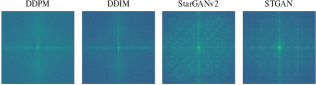
(a) Frequency artifacts in different forgery methods. DDPM [25] and DDIM [64] do not exhbit the checkboard patterns [78, 68] observed in GAN-based methods, such as StarGAN-v$2$ [12] and STGAN [44].

Table 3: IFDL Results on HiFi-IFDL. $*$ means we apply author-released pre-trained models. Models without $*$ mean they are trained on HiFi-IFDL training set. [Bold: best result].

\begin{overpic}[width=472.01192pt]{results/loc_figure} \put(-1.0,27.5){Image} \put(1.0,19.0){\small{GT}} \put(-0.5,12.5){\small{PSCC}} \put(0.5,10.5){\small{\cite[cite]{[\@@bibref{}{liu2022pscc}{}{}]}}} \put(0.0,4.0){\small{Ours}} \end{overpic}

Figure 8: Qualitative results on different forged images. The first $6$ columns are from image editing methods whereas the last $3$ columns are images generated by Faceshifer [38] and STGAN [44].

Localization	Col.	Cov.	NI.$16$	CAS.	IM$20$	Avg.
	Metric: AUC($\%$) – Pre-trained
ManT.[73]	$82.4$	$81.9$	$79.5$	$81.7$	$74.8$	$80.0$
SPAN[27]	$93.6$	$92.2$	$84.0$	$79.7$	$75.0$	$84.9$
PSCC[45]	$98.2$	$84.7$	$85.5$	$82.9$	$80.6$	$86.3$
Ob.Fo.[67]	$95.5$	$\color[rgb]{0,0,1}92.8$	$\mathbf{\color[rgb]{1,0,0}{87.2}}$	$84.3$	$82.1$	$88.3$
Ours∗	$\color[rgb]{0,0,1}{98.3}$	$\mathbf{\color[rgb]{1,0,0}{93.2}}$	$\color[rgb]{0,0,1}{87.0}$	$\color[rgb]{0,0,1}{85.8}$	$\color[rgb]{0,0,1}{82.9}$	$\color[rgb]{0,0,1}{89.4}$
Ours	$\mathbf{\color[rgb]{1,0,0}98.4}$	92.4	$86.9$	$\mathbf{\color[rgb]{1,0,0}86.6}$	$\mathbf{\color[rgb]{1,0,0}83.4}$	$\mathbf{\color[rgb]{1,0,0}89.6}$

(a)

Localization	Cov.	CAS.	NI.$16$	Avg.
	Metric: AUC($\%$) / F$1$($\%$) – Fine-tuned
SPAN[27]	$93.7/55.8$	$83.8/40.8$	$96.1/58.2$	$91.2/51.6$
PSCC[45]	$94.1/72.3$	$87.5/55.4$	$\color[rgb]{1,0,0}\mathbf{99.6}$/$81.9$	$93.7/69.8$
Ob.Fo.[67]	$\color[rgb]{0,0,1}95.7$/$\color[rgb]{0,0,1}75.8$	$\color[rgb]{0,0,1}88.2$/$\color[rgb]{0,0,1}57.9$	$\color[rgb]{0,0,1}99.6$/$\color[rgb]{0,0,1}82.4$	$\color[rgb]{0,0,1}{94.5}$/$\color[rgb]{0,0,1}72.0$
Ours	$\color[rgb]{1,0,0}{\mathbf{96.1}}$/$\mathbf{\color[rgb]{1,0,0}{80.1}}$	$\color[rgb]{1,0,0}\mathbf{88.5}$/$\color[rgb]{1,0,0}\mathbf{61.6}$	$98.9$/$\color[rgb]{1,0,0}\mathbf{85.0}$	$\color[rgb]{1,0,0}\mathbf{94.6}$/$\color[rgb]{1,0,0}\mathbf{75.5}$

(b)

Detection	AUC(%)	F$1$(%)
ManT.[73]	$59.9$	$56.7$
SPAN[27]	$67.3$	$63.8$
PSCC[45]	$99.5$	$97.1$
Ob.Fo.[67]	$\color[rgb]{1,0,0}\mathbf{99.7}$	$\color[rgb]{0,0,1}97.3$
Ours	$\color[rgb]{0,0,1}99.5$	$\color[rgb]{1,0,0}\mathbf{97.4}$

(c)

Table 4: IFDL results on the image editing. (a) Localization performance of the pre-train model. (b) Localization performance of the fine-tuned model. (c) Detection performance on CASIA dataset. All results of prior works are ported from [67]. [Key: Best; Second Best; Ours^∗ uses the same pre-trained dataset as [45], and ours is pre-trained on HiFi-IFDL].

5.1 Image Forgery Detection and Localization

5.1.1 HiFi-IFDL Dataset

Tab. 3 reports the different model performance on the HiFi-IFDL dataset, in which we use AUC and F$1$ score as metrics on both image-level forgery detection and pixel-level localization. Specifically, in Tab. 3(a), first we observe that the pre-trained CNN-detector [68] does not perform well because it is trained on GAN-generated images that are different from images manipulated by diffusion models. Such differences can be seen in Fig. 8(a), where we visualize the frequency domain artifacts, by following the routine [68] that applies the high-pass filter on the image generated by different forgery methods. Similar visualization is adopted in [68, 78, 13, 56] also. Then, we train both prior methods on HiFi-IFDL, and they again perform worse than our model: CNN-detector uses ordinary ResNet$50$, but our model is specifically designed for image forensics. Two-branch processes deepfakes video by LSTM that is less effective to detect forgery in image editing domain. Attention Xception [65] and PSCC [45] are proposed for facial image forgery and image editing domain, respectively. These two methods perform worse than us by $9.3\%$ and $3.6\%$ AUC, respectively. We believe this is because our method can leverage localization results to help the image-level detection.

In Tab. 3(b), we compare with previous methods which can perform the forgery localization. Specifically, the pre-trained OSN-detector [74] and CatNet [36] do not work well on CNN-synthesized images in HiFi-IFDL dataset, since they merely train models on images manipulated by editing methods. Then, we use HiFi-IFDL dataset to train CatNet, but it still performs worse than ours: CatNet uses DCT stream to help localize area of splicing and copy-move, but HiFi-IFDL contains more forgery types (e.g., inpainting). Meanwhile, the accurate classification performance further helps the localization as statistics and patterns of forgery regions are related to different individual forgery method. For example, for the forgery localization, we achieve $2.6\%$ AUC and $2.0\%$ F$1$ improvement over PSCC. Additionally, the superior localization demonstrates that our hierarchical fine-grained formulation learns more comprehensive forgery localization features than multi-level localization scheme proposed in PSCC.

5.1.2 Image Editing Datasets

Tab. 4 reports IFDL results for the image editing domain. We evaluate on $5$ datasets: Columbia [51], Coverage [71], CASIA [19], NIST16 [2] and IMD$20$ [53]. Following the previous experimental setup of [73, 27, 45, 18, 67], we pre-train the model on our proposed HiFi-IFDL and then fine-tune the pre-trained model on the NIST16, Coverage and CASIA. We also report the performance of HiFi-Net pre-trained on the same dataset as  [45]. Tab. 4(a) reports the pre-trained model performance, in which our method achieves the best average performance. The ObjectFormer [67] adopts the powerful transformer-based architecture and solely specializes in forgery detection of the image editing domain, nevertheless its performance are on-par with ours. In the fine-tune stage, our method achieves the best performance on average AUC and F$1$. Specifically, we only fall behind on NIST16, where AUC tends to saturate. We also report the image-level forgery detection results in Tab. 4(c), achieving comparable results to ObjectFormer [67]. We show qualitative results in Fig. 8, where the manipulated region identified by our method can capture semantically meaningful object shape, such as the shapes of the tiger and squirrel. At last, we also offer the robustness evaluation in Tab. 2 of the supplementary, showing our performance against various image transformations.

Metric: IoU / PBCA
Att.Xce. [65]	$0.401/0.786$
Ours	$\mathbf{0.411}/\mathbf{0.801}$

(a) localization

Metric: AUC/PBCA
Att.Xce. [65]	$\mathbf{99.69}/88.44$
Ours	$99.45/\mathbf{88.50}$

(b) detection

Table 5: IFDL results on DFFD dataset. [Key: Best]

5.1.3 Diverse Fake Face Dataset

We evaluate our method on the Diverse Fake Face Dataset (DFFD) [65]. For a fair comparison, we follow the same experiment setup and metrics: IoU and pixel-wise binary classification accuracy (PBCA) for pixel-level localization, and AUC and PBCA for image-level detection. Tab. 5 reports that our method obtains competitive performance on detection and the best localization performance on partial-manipulated images. More results are in the appendix.

5.2 Ablation Study

In row $1$ and $2$ of Tab. 6, we first ablate the $\mathcal{L}_{loc}$ and $\mathcal{L}_{cls}$, removing which causes large performance drops on the detection ($24.1\%$ F$1$) and localization ($29.3\%$ AUC), respectively. Also, removing $\mathcal{L}_{cls}$ harms localization by $1.9\%$ AUC and F$1$. This shows that fine-grained classification improves the localization, as the fine-grained classification features serve as a prior for localization. We evaluate the effectiveness of performing fine-grained classification at different hierarchical levels. In the $3$th row, we only keep the $4$th level fine-grained classification in the training, which causes a sensible drop of performance in detection ($3.7\%$ AUC) and localization ($2.8\%$ AUC). In the $4$th row, we perform the fine-grained classification without forcing the dependency between layers of Eq. 4. This impairs the learning of hierarchical forgery attributes and causes a drop of $3.6\%$ AUC in the detection. Lastly, we ablate the PConv in the $5$th row, making model less effective for detection.

	Method	Loss	Detection		Localization
			AUC	F$1$	AUC	F$1$
Full	M,L,P	$\mathcal{L}_{cls}$, $\mathcal{L}_{loc}$	$\mathbf{96.8}$	$\mathbf{94.1}$	$\mathbf{95.3}$	$\mathbf{96.9}$
1	M,L,P	$\mathcal{L}_{loc}$	$65.0$	$70.0$	$93.4$	$95.0$
2	M,L,P	$\mathcal{L}_{cls}$	$95.8$	$92.4$	$66.0$	$58.0$
3	M,L,P	$\mathcal{L}^{4}_{cls}$,$\mathcal{L}_{loc}$	$93.1$	$91.7$	$92.5$	$93.9$
4	M,L,P	$\mathcal{L}^{ind}_{cls}$,$\mathcal{L}_{loc}$	$93.2$	$92.8$	$93.2$	$94.8$
5	M,L	$\mathcal{L}_{cls},\mathcal{L}_{loc}$	$96.6$	$93.0$	$94.8$	$96.0$

Table 6: Ablation study. M, L, and P represent the multi-branch classification module, localization module and Pconv operation, respectively. $\mathcal{L}_{cls}$ and $\mathcal{L}_{loc}$ are classification and localization loss, respectively. $\mathcal{L}^{4}_{cls}$ and $\mathcal{L}^{ind}_{cls}$ denote we only perform the fine-grained classification on $4^{th}$ level and classification without hierarchical path prediction. [Key: Best]

	F$1$ score
Attr. [76]	$31.11$
FEN [6]	$48.00$
Baseline	$84.62$
Multi-scale	$85.37$
HiFi-Net	$\mathbf{87.63}$

(a)

\begin{overpic}[width=433.62pt]{results/confusion_matrix.pdf} \put(-13.0,14.0){\small\rotatebox{90.0}{True Label}} \put(-10.0,72.0){\scriptsize{Real}} \put(-13.0,65.5){\scriptsize{Splice}} \put(-15.0,59.5){\scriptsize{Inpaint}} \put(-6.0,55.0){\tiny{\cite[cite]{[\@@bibref{}{liu2019stgan}{}{}]}}} \put(-6.0,49.0){\tiny{\cite[cite]{[\@@bibref{}{liu2019stgan}{}{}]}}} \put(-6.0,44.0){\tiny{\cite[cite]{[\@@bibref{}{li2019faceshifter}{}{}]}}} \put(-6.0,38.0){\tiny{\cite[cite]{[\@@bibref{}{choi2020starganv2}{}{}]}}} \put(-6.0,33.0){\tiny{\cite[cite]{[\@@bibref{}{li2021image_hisd}{}{}]}}} \put(-6.0,28.0){\tiny{\cite[cite]{[\@@bibref{}{karras2020training_styleGan2ADA}{}{}]}}} \put(-6.0,23.0){\tiny{\cite[cite]{[\@@bibref{}{karras2021alias_styleGan3}{}{}]}}} \put(-6.0,18.0){\tiny{\cite[cite]{[\@@bibref{}{ho2020denoising_ddpm}{}{}]}}} \put(-6.0,13.0){\tiny{\cite[cite]{[\@@bibref{}{song2020denoising_ddim}{}{}]}}} \put(-6.0,8.0){\tiny{\cite[cite]{[\@@bibref{}{nichol2021glide}{}{}]}}} \put(-6.0,3.0){\tiny{\cite[cite]{[\@@bibref{}{rombach2021highresolution_latent_diffusion}{}{}]}}} \end{overpic}

(a)

Figure 9: (a) The forgery attribute classification results. The improvement over previous works [76, 6] is because the previous works only learn to attribute CNN-synthesized images, yet do not consider attributing image editing methods. (b) The confusion matrix of forgery attribute classification at level $4$, where a, b and c represent three scenarios of classification failures. The numerical value indicates the accuracy. See Sec. 5.3 and Fig. 10 for details.

5.3 Forgery Attribute performance

We perform the fine-grained classification among real images and $13$ forgery categories on $4$ different levels, and the most challenging scenario is the fine-grained classification on the $4$ th level. The result is reported in Tab. 7(a). Specifically, we train HiFi-Net $4$ times, and at each time only classifies the fine-grained forgery attributes at one level, denoted as Baseline. Then, we train a HiFi-Net to classify all $4$ levels but without the hierarchical dependency via Eq. 4, denoted as multi-scale. Also, we compare to the pre-trained image attribution works [6, 76]. Also, it has been observed in Fig. 9(a) that we fail on $3$ scenarios 1) Some real images have watermarks, extreme lightings, and distortion. 2) Inpainted images have small forgery regions. 3) styleGANv$2$-ada [31] and styleGAN$3$ [32] can produce highly similar images. Fig. 10 shows failure cases.

\begin{overpic}[width=218.61795pt]{results/gallery.pdf} \put(-5.0,60.0){(a)} \put(-5.0,40.0){(b)} \put(-5.0,15.0){(c)} \end{overpic}

Figure 10: Three failure scenarios: (a) real images. (b) inpainting images with small removal regions. (c) images generated from different styleGANv$2$ada [31] and styleGANv$3$ [32], as shown in the last two rows, respectively.

6 Conclusion

In this work, we develop a method for both CNN-synthesized and image editing forgery domains. We formulate the IFDL as a hierarchical fine-grained classification problem which requires the algorithm to classify the individual forgery method of given images, via predicting the entire hierarchical path. Also, HiFi-IFDL dataset is proposed to further help the community in developing forgery detection algorithms.

Limitation

Please refer to the supplementary Sec. 2: the model that performs well on the conventional image editing can generalize poorly on diffusion-based inpainting method. Secondly, we think it is possible improve the IFDL learning via the larger forgery dataset.

7 Supplementary

In this supplementary material, we include many details of our work: 1) the details of the proposed HiFi-IFDL dataset; 2) The generalization performance against images generated from unseen forgery methods and real images in the unseen domain; 3) the HiFi-Net performance against different types of post-processing in the image editing domain; 4) the complete HiFi-Net performance on the DFFD dataset [65]; 5) we offer the forgery attribute classification results on seen and unseen forgery attributes; 6). the detailed implementation of the proposed HiFi-Net.

7.1 Dataset Collection Details

Table 7 reports all the forgery methods used in our dataset. In the last column, the table shows if the method used to generate the manipulated images is pre-trained, self-trained, or we used the released images. In Fig. 14 and Fig. 15, we show several examples taken from our dataset that represents a variety of objects, scenes, faces, animals. The real image dataset is the combination of LSUN [75], CelebaHQ [37], FFHQ [33], AFHQ [12], MSCOCO [41] and real face images in face forensics [58]. We either take the entire dataset or randomly select $100$k images from these real datasets.

Forgery Method	Image Source	Images $\#$	Source
DDPM [25]	LSUN	$100$k	pre-trained
DDIM [64]	LSUN	$100$k	pre-trained
GDM. [52]	LSUN	$100$k	pre-trained
LDM. [57]	LSUN	$100$k	pre-trained
StarGANv$2$ [12]	CelebaHQ	$100$k	pre-trained
HiSD [40]	CelebaHQ	$100$k	pre-trained
StGANv$2$-ada [31]	FFHQ, AFHQ	$100$k	pre-trained
StGAN$3$ [32]	FFHQ, AFHQ	$100$k	pre-trained
STGAN [44]	CelebaHQ	$100$k	self-train
Faceshifter [38]	Youtube video	$100$k	released

Table 7: The details of the collected dataset. Each column in order shows forgery method; the image source used for the generation; the image number; if the images are generated with a pre-trained/self-trained models or released images.

7.2 Generalization Performance

\begin{overpic}[scale={0.35}]{results/generalization.pdf} \put(10.0,0.0){\tiny{ProGAN}} \put(12.0,-3.0){\scriptsize{\cite[cite]{[\@@bibref{}{karras2018progressive}{}{}]}}} \put(20.0,0.0){\tiny{StyGAN}} \put(21.0,-3.0){\scriptsize{\cite[cite]{[\@@bibref{}{karras2019style}{}{}]}}} \put(30.0,0.0){\tiny{DPGAN}} \put(31.0,-3.0){\scriptsize{\cite[cite]{[\@@bibref{}{wang2022diffusion}{}{}]}}} \put(40.0,0.0){\tiny{DSGAN}} \put(41.0,-3.0){\scriptsize{\cite[cite]{[\@@bibref{}{wang2022diffusion}{}{}]}}} \put(50.0,0.0){\tiny{ADM}} \put(51.0,-3.0){\scriptsize{\cite[cite]{[\@@bibref{}{dhariwal2021diffusion}{}{}]}}} \put(60.0,0.0){\tiny{PNDM}} \put(61.0,-3.0){\scriptsize{\cite[cite]{[\@@bibref{}{liu2022pseudo}{}{}]}}} \put(70.0,0.0){\tiny{SiWM-v2}} \put(71.0,-3.0){\scriptsize{\cite[cite]{[\@@bibref{}{guo2022multi}{}{}]}}} \put(80.0,0.0){\tiny{RePaint}} \put(80.0,-3.0){\scriptsize{\cite[cite]{[\@@bibref{}{lugmayr2022repaint}{}{}]}}} \put(90.0,0.0){\tiny{LDM}} \put(90.0,-3.0){\scriptsize{\cite[cite]{[\@@bibref{}{rombach2021highresolution_latent_diffusion}{}{}]}}} \end{overpic}

Figure 11: The image-level forgery detection accuracy on images generated by unseen GAN ( ) and diffusion ( ) methods, and unseen domain real images ( ). The pixel-level localization accuracy on images inpainted by unseen diffusion model ( ). From left to right, first $6$ methods produce bedroom in LSUN [75]. The SiW-Mv$2$ contains real human face. Images generated from the last two diffusion model inpainting methods, are human face and general objects. All these images are either obtained directly from the open source github or the pre-trained weight.

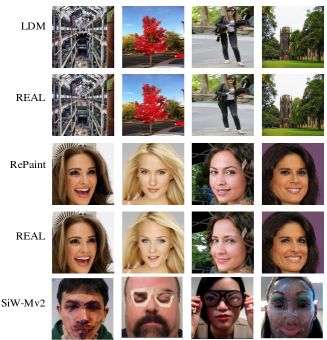
Figure 12: Images manipulated by LDM [57] and RePaint [46] and their corresponding real images. The last row is the SiW-Mv$2$ dataset, where real human faces have spoof traces, such as funnyeyes and masks.

Fig. 11 reports our method’s generalization performance. Specifically, for each generative method and unseen domain real images, we have collected $1000$ images and use these images to form an inference dataset. After that, we apply the pre-trained HiFi-Net on such an inference to compute the classification accuracy, given $0.5$ fixed-threshold.

Our first conclusion is the same as the most recent work [56] that some generative methods such as DSGAN [70] and PNDM [43] can generate rather sophisticated images that fool the powerful forgery detector.

Secondly, we hypothesize that powerful forgery detector can largely fail when being applied on real images in different domain. For example, real images from SiW-Mv$2$ dataset [22], where facial image has spoof traces, such as funny glasses and wigs.

Lastly, and more importantly, we observe the well-trained model always generalizes poorly on the image that is partially manipulated by diffusion model. We think this is because of two reasons: (1) conventional image editing methods are distinct by nature to the most recently proposed inpainting methods based on diffusion model; (2) the forgery area edited by diffusion model can have variations, not a rigid copy-move or removal manner that is commonly used by the traditional editing methods.

We believe these three aspects are valuable for the future research, namely: (a) how to make the model generalize well on detecting forged images created by advanced methods, (b) how to maintain the precision when we have real images from the new domain, (c) diffusion model based inpanting method can raise an issue for the existing forgery localization methods, indicating that new algorithm is needed.

7.3 Image Editing Experiment

Following previous works [67, 45, 27], we evaluate the performance of our method against different post-processing steps, which is reported in Tab. 8. Our proposed method is more robust than the previous work, except for the post-processing of resizing $0.78$ times the image and JPEG compression with $50\%$ quality. Meanwhile, more qualitative results can be found in Fig. 16.

Post.	SPAN [27]	PSCC [45]	Obj.Fo. [67]	Ours
Resize ($0.78$)	$83.24$	$85.29$	$\mathbf{87.2}$	$86.9$
Resize ($0.25$)	$80.32$	$85.01$	$86.3$	$\mathbf{86.5}$
Gau.Blur ($3$)	$83.10$	$85.38$	$85.97$	$\mathbf{86.1}$
Gau.Blur ($15$)	$79.15$	$79.93$	$80.26$	$\mathbf{81.0}$
Gau.Noi ($3$)	$75.17$	$78.42$	$79.58$	$\mathbf{81.9}$
Gau.Noi ($15$)	$67.28$	$76.65$	$78.15$	$\mathbf{79.5}$
JPEG Co. ($100$)	$83.59$	$85.40$	$86.37$	$\mathbf{86.5}$
JPEG Co. ($50$)	$80.68$	$85.37$	$\mathbf{86.24}$	$86.0$

Table 8: IFDL performance on NIST16 with different post-processing steps. [Key: Best; Gau.: Gaussian; JPEG Co.: JPEG Compression.].

7.4 The DFFD Dataset Performance

We have included the complete version of our method performance on the DFFD dataset in Tab. 9. As we can see, compared to Attention Xception [65], our method still achieves more accurate localization performance on Partial Manipulated and Fully Synthesized images. For the localization performance on the real images, our performance is comparable with the Attention Xception [65].

IoU ($\uparrow$) / PBCA ($\uparrow$)	Real	Fu. Syn.	Par. Man.
Att. [65]	$-/\mathbf{0.998}$	$0.847/0.847$	$0.401/0.786$
Ours	$-/0.978$	$\mathbf{0.893}/\mathbf{0.893}$	$\mathbf{0.411}/\mathbf{0.801}$

(a)

IINC ($\downarrow$) / C.S. ($\downarrow$)	Real	Fu. Syn.	Par. Man.
Att. [65]	$0.015/-$	$0.077/\mathbf{0.095}$	$\mathbf{0.311}/0.429$
Ours	$\mathbf{0.010}/-$	$\mathbf{0.060}/0.107$	$0.323/\mathbf{0.410}$

(b)

Table 9: The localization performance: (a) Metrics are IoU and PBCA, the higher the better, (b) Metrics are IINC and Cosine Similarity, the lower the better. [Keys: Fu. Syn.: Fully-synthesized; Par. Man.: Partially-manipulated]

\begin{overpic}[width=496.85625pt]{results/prob.pdf} \end{overpic}

Figure 13: (a) The original hierarchical structure used in the fine-grained classification at different levels. (b). For convenience, we assign category number to each forgery attribute, at different levels. (c). The detailed prediction probability for each input forged images. The table below each image reports the categorical value $\hat{\mathbf{y}}_{b}$ and corresponding prediction probability $p(\mathbf{y}_{b}|\mathbf{X})$. From the top to down order, the results shown are for level$1$ to level$4$. For example, in the splicing image (example ($1$)): partial manipulated$\rightarrow$image editing$\rightarrow$image editing$\rightarrow$splicing, which corresponds to the label index $1,3,5,10$ that are shown in the first table. Lastly, the example ($1$) – ($10$) are seen forgery method in the training, and the example ($11$) and ($12$) are unseen forgery attribute.

7.5 Forgery Attribute Classification

We have included specific classification results for a variety of samples. Tab. (6) of the paper reports the fine-grained classification result of HiFi-IFDL. Here we show the classification probability at different levels. In examples ($5$) and ($10$) of Fig. 13, we can see the robustness of our proposed method that learns the hierarchical structure. The $3$rd level fine-grained prediction probability on $5$th example and $10$th example is lower than the fine-grained classification prediction probability on the $4$th level. This means our algorithm can recover the accuracy at the fine level classification even the classification on the coarser level does not perform excellent.

7.6 Implementation Details

In our HiFi-Net, the feature map resolution for different branches are $256$, $128$, $64$, and $32$ pixels. In the experiment on HiFi-IFDL, the fine-grained classification for $1$st, $2$nd, $3$rd and $4$th levels are $2$-way, $4$-way, $6$-way and $14$-way multi-class classification, respectively. The $3$rd level fine-grained classification categories are: unconditional diffusion, conditional diffusion, unconditional GAN, conditional GAN, CNN-based partial manipulation and Image editing.

As for the details of $\mathcal{L}_{loc}$ implementation, we first use the initialized HiFi-Net to convert each pixel in the input image to the high-dimensional feature $\mathbf{F}^{\prime}_{ij}\in R^{D}$, where $D=18$. Then we average the feature $\mathbf{F}^{\prime}_{ij}\in R^{D}$ for all pixels in the real image from the HiFi-IFDL, and this average value then is used as $\mathbf{c}$. Then, we compute the $\ell_{2}$ distance between each pixel feature $\mathbf{F}^{\prime}_{ij}\in R^{D}$ and $\mathbf{c}$, and denote the largest distance as $D_{max}$. In the Eq. (1) of the paper, we set the threshold $\tau$ as $2.5\cdot D_{max}$.

The architecture is trained end-to-end with different learning rates per layers. The detailed objective function is:

$$\small\mathcal{L}_{tot}=\begin{cases}$100*$\mathcal{L}_{loc}+\mathcal{L}^{1}_{cls}+\mathcal{L}^{2}_{cls}+\mathcal{L}^{3}_{cls}+$100*$\mathcal{L}^{4}_{cls}&\mbox{if $\mathbf{X}$ is forged}\\ \mathcal{L}_{loc}+\mathcal{L}^{4}_{cls}&\mbox{if $\mathbf{X}$ is real}\end{cases}$$

Where $\mathbf{X}$ is the input image. When the input image is labeled as “real”, we only apply the last branch ($\boldsymbol{\theta}_{4}$) loss function, otherwise, if it is labeled as “manipulated”, we use all the branches.

The entire architecture is trained for $13$ epoches, and all training samples are seen by the model in each epoch. The feature extractor is modified based on the pre-trained HRNet [66], in which we add more layers such that each branch of our multi-branch feature extractor can have identical number of convolutional layers, and the details can be found in our source code that will be released upon the acceptance. We use 1e-4 to train the multi-branch feature extractor and classification module, and 3e-4 to train the localization modules. During the training, we use ReduceLROnPlateau as the learning rate scheduler to reduce the learning rate.

7.7 Societal Impact

Our work has the positive societal impact to the community. Because our work is dealing with various categories of forgery methods, which enable the algorithm to detect all kinds of manipulation, including seen and unseen forgeries, as indicated by Supplementary section 4. Our algorithm can enable a tool that makes general public in our society to have more trust in media contents.

\begin{overpic}[width=496.85625pt]{results/dataset_1.pdf} \end{overpic}

Figure 14: The samples from the proposed HiFi-IFDL dataset. From top to bottom, the images are generated by DDPM, DDIM, LDM, GDM, StarGANv$2$, HiSD, StyleGANv$2$ada, StyleGANv$3$.

\begin{overpic}[width=496.85625pt]{results/dataset_2.pdf} \end{overpic}

Figure 15: Additional samples from the proposed HiFi-IFDL dataset. From top to bottom, the images are generated by STGAN, Faceshifter, and two image editing methods.

\begin{overpic}[width=496.85625pt]{results/supp_res.pdf} \end{overpic}

Figure 16: Additional qualitative results on CASIA, NIST16 and Coverage dataset.

References

- [1] Survey: More americans get news from internet than newspapers or radio. http://www.cnn.com/2010/TECH/03/01/social.network.news/index.html.
- [2] Nist: Nist nimble 2016 datasets., May 2016.
- [3] Infodemic - world Health Organization. https://www.who.int/health-topics/infodemic, 2022.
- [4] Wael AbdAlmageed, Hengameh Mirzaalian, Xiao Guo, Linda M Randolph, Veeraya K Tanawattanacharoen, Mitchell E Geffner, Heather M Ross, and Mimi S Kim. Assessment of facial morphologic features in patients with congenital adrenal hyperplasia using deep learning. JAMA network open, 2020.
- [5] Vishal Asnani, Xi Yin, Tal Hassner, Sijia Liu, and Xiaoming Liu. Proactive image manipulation detection. In CVPR, 2022.
- [6] Vishal Asnani, Xi Yin, Tal Hassner, and Xiaoming Liu. Reverse engineering of generative models: Inferring model hyperparameters from generated images. arXiv preprint arXiv:2106.07873, 2021.
- [7] Vishal Asnani, Xi Yin, Tal Hassner, and Xiaoming Liu. Malp: Manipulation localization using a proactive scheme. In CVPR, 2023.
- [8] Tu Bui, Ning Yu, and John Collomosse. Repmix: Representation mixing for robust attribution of synthesized images. In ECCV, 2022.
- [9] Peter J Burt and Edward H Adelson. The laplacian pyramid as a compact image code. In Readings in computer vision. Elsevier, 1987.
- [10] Lucy Chai, David Bau, Ser-Nam Lim, and Phillip Isola. What makes fake images detectable? understanding properties that generalize. In ECCV, 2020.
- [11] Xinru Chen, Chengbo Dong, Jiaqi Ji, Juan Cao, and Xirong Li. Image manipulation detection by multi-view multi-scale supervision. In ICCV, 2021.
- [12] Yunjey Choi, Youngjung Uh, Jaejun Yoo, and Jung-Woo Ha. Stargan v2: Diverse image synthesis for multiple domains. In CVPR, 2020.
- [13] Riccardo Corvi, Davide Cozzolino, Giada Zingarini, Giovanni Poggi, Koki Nagano, and Luisa Verdoliva. On the detection of synthetic images generated by diffusion models. arXiv preprint arXiv:2211.00680, 2022.
- [14] Davide Cozzolino, Justus Thies, Andreas Rössler, Christian Riess, Matthias Nießner, and Luisa Verdoliva. Forensictransfer: Weakly-supervised domain adaptation for forgery detection. arXiv preprint arXiv:1812.02510, 2018.
- [15] Debayan Deb, Xiaoming Liu, and Anil Jain. Unified detection of digital and physical face attacks. In FG, 2023.
- [16] Prafulla Dhariwal and Alexander Nichol. Diffusion models beat gans on image synthesis. 2021.
- [17] Brian Dolhansky, Russ Howes, Ben Pflaum, Nicole Baram, and Cristian Canton Ferrer. The Deepfake Detection Challenge (DFDC) Preview Dataset. arXiv preprint arXiv: 1910.08854, 2019.
- [18] Chengbo Dong, Xinru Chen, Ruohan Hu, Juan Cao, and Xirong Li. Mvss-net: Multi-view multi-scale supervised networks for image manipulation detection. TPAMI, 2022.
- [19] Jing Dong, Wei Wang, and Tieniu Tan. Casia image tampering detection evaluation database. 2013 IEEE China Summit and ICSIP, 2013.
- [20] Nicholas Dufour, Andrew Gully, Per Karlsson, Alexey Victor Vorbyov, Thomas Leung, Jeremiah Childs, and Christoph Bregler. Deepfakes detection dataset by Google & Jigsaw, 2019.
- [21] Xiao Guo and Jongmoo Choi. Human motion prediction via learning local structure representations and temporal dependencies. In AAAI, 2019.
- [22] Xiao Guo, Yaojie Liu, Anil Jain, and Xiaoming Liu. Multi-domain learning for updating face anti-spoofing models. In ECCV, 2022.
- [23] Xiao Guo, Hengameh Mirzaalian, Ekraam Sabir, Ayush Jaiswal, and Wael Abd-Almageed. Cord19sts: Covid-19 semantic textual similarity dataset. arXiv preprint arXiv:2007.02461, 2020.
- [24] Jonathan Ho, William Chan, Chitwan Saharia, Jay Whang, Ruiqi Gao, Alexey Gritsenko, Diederik P Kingma, Ben Poole, Mohammad Norouzi, David J Fleet, et al. Imagen video: High definition video generation with diffusion models. arXiv preprint arXiv:2210.02303, 2022.
- [25] Jonathan Ho, Ajay Jain, and Pieter Abbeel. Denoising diffusion probabilistic models. In NeurIPS, 2020.
- [26] I Hsu, Xiao Guo, Premkumar Natarajan, Nanyun Peng, et al. Discourse-level relation extraction via graph pooling. In AAAI DLG Wrokshop, 2021.
- [27] Xuefeng Hu, Zhihan Zhang, Zhenye Jiang, Syomantak Chaudhuri, Zhenheng Yang, and Ram Nevatia. Span: spatial pyramid attention network for image manipulation localization. In ECCV, 2020.
- [28] Yihao Huang, Felix Juefei-Xu, Qing Guo, Yang Liu, and Geguang Pu. Fakelocator: Robust localization of gan-based face manipulations. TIFS, 2022.
- [29] Liming Jiang, Ren Li, Wayne Wu, Chen Qian, and Chen Change Loy. Deeperforensics-1.0: A large-scale dataset for real-world face forgery detection. In CVPR, 2020.
- [30] Tero Karras, Timo Aila, Samuli Laine, and Jaakko Lehtinen. Progressive growing of gans for improved quality, stability, and variation. In ICLR, 2018.
- [31] Tero Karras, Miika Aittala, Janne Hellsten, Samuli Laine, Jaakko Lehtinen, and Timo Aila. Training generative adversarial networks with limited data. In NeurIPS, 2020.
- [32] Tero Karras, Miika Aittala, Samuli Laine, Erik Härkönen, Janne Hellsten, Jaakko Lehtinen, and Timo Aila. Alias-free generative adversarial networks. In NeurIPS, 2021.
- [33] Tero Karras, Samuli Laine, and Timo Aila. A style-based generator architecture for generative adversarial networks. In CVPR, 2019.
- [34] Diederik P Kingma and Max Welling. Auto-encoding variational bayes. In ICLR, 2014.
- [35] Pavel Korshunov and Sebastien Marcel. Vulnerability assessment and detection of deepfake videos. In ICB, 2019.
- [36] Myung-Joon Kwon, Seung-Hun Nam, In-Jae Yu, Heung-Kyu Lee, and Changick Kim. Learning jpeg compression artifacts for image manipulation detection and localization. IJCV, 2022.
- [37] Cheng-Han Lee, Ziwei Liu, Lingyun Wu, and Ping Luo. Maskgan: Towards diverse and interactive facial image manipulation. In CVPR, 2020.
- [38] Lingzhi Li, Jianmin Bao, Hao Yang, Dong Chen, and Fang Wen. Faceshifter: Towards high fidelity and occlusion aware face swapping. In CVPR, 2020.
- [39] Lingzhi Li, Jianmin Bao, Ting Zhang, Hao Yang, Dong Chen, Fang Wen, and Baining Guo. Face x-ray for more general face forgery detection. In CVPR, 2020.
- [40] Xinyang Li, Shengchuan Zhang, Jie Hu, Liujuan Cao, Xiaopeng Hong, Xudong Mao, Feiyue Huang, Yongjian Wu, and Rongrong Ji. Image-to-image translation via hierarchical style disentanglement. In CVPR, 2022.
- [41] Tsung-Yi Lin, Michael Maire, Serge Belongie, James Hays, Pietro Perona, Deva Ramanan, Piotr Dollár, and C Lawrence Zitnick. Microsoft coco: Common objects in context. In ECCV, 2014.
- [42] Guilin Liu, Fitsum A Reda, Kevin J Shih, Ting-Chun Wang, Andrew Tao, and Bryan Catanzaro. Image inpainting for irregular holes using partial convolutions. In ECCV, 2018.
- [43] Luping Liu, Yi Ren, Zhijie Lin, and Zhou Zhao. Pseudo numerical methods for diffusion models on manifolds. 2022.
- [44] Ming Liu, Yukang Ding, Min Xia, Xiao Liu, Errui Ding, Wangmeng Zuo, and Shilei Wen. Stgan: A unified selective transfer network for arbitrary image attribute editing. In CVPR, 2019.
- [45] Xiaohong Liu, Yaojie Liu, Jun Chen, and Xiaoming Liu. Pscc-net: Progressive spatio-channel correlation network for image manipulation detection and localization. TCSVT, 2022.
- [46] Andreas Lugmayr, Martin Danelljan, Andres Romero, Fisher Yu, Radu Timofte, and Luc Van Gool. Repaint: Inpainting using denoising diffusion probabilistic models. In CVPR, 2022.
- [47] Francesco Marra, Diego Gragnaniello, Davide Cozzolino, and Luisa Verdoliva. Detection of gan-generated fake images over social networks. In MIPR, 2018.
- [48] Francesco Marra, Diego Gragnaniello, Luisa Verdoliva, and Giovanni Poggi. Do gans leave artificial fingerprints? In MIPR, 2019.
- [49] Iacopo Masi, Aditya Killekar, Royston Marian Mascarenhas, Shenoy Pratik Gurudatt, and Wael AbdAlmageed. Two-branch recurrent network for isolating deepfakes in videos. In ECCV, 2020.
- [50] Owen Mayer and Matthew C Stamm. Learned forensic source similarity for unknown camera models. In ICASSP, 2018.
- [51] Tian-Tsong Ng, Jessie Hsu, and Shih-Fu Chang. Columbia image splicing detection evaluation dataset. DVMM lab. Columbia Univ CalPhotos Digit Libr, 2009.
- [52] Alex Nichol, Prafulla Dhariwal, Aditya Ramesh, Pranav Shyam, Pamela Mishkin, Bob McGrew, Ilya Sutskever, and Mark Chen. Glide: Towards photorealistic image generation and editing with text-guided diffusion models. In ICML, 2021.
- [53] Adam Novozamsky, Babak Mahdian, and Stanislav Saic. Imd2020: A large-scale annotated dataset tailored for detecting manipulated images. In WACV Workshop, 2020.
- [54] Patrick Pérez, Michel Gangnet, and Andrew Blake. Poisson image editing. ACM SIGGRAPH, 2003.
- [55] Aditya Ramesh, Prafulla Dhariwal, Alex Nichol, Casey Chu, and Mark Chen. Hierarchical text-conditional image generation with clip latents. arXiv preprint arXiv:2204.06125, 2022.
- [56] Jonas Ricker, Simon Damm, Thorsten Holz, and Asja Fischer. Towards the detection of diffusion model deepfakes. arXiv preprint arXiv:2210.14571, 2022.
- [57] Robin Rombach, Andreas Blattmann, Dominik Lorenz, Patrick Esser, and Björn Ommer. High-resolution image synthesis with latent diffusion models. In CVPR, 2022.
- [58] Andreas Rössler, Davide Cozzolino, Luisa Verdoliva, Christian Riess, Justus Thies, and Matthias Nießner. Faceforensics++: Learning to detect manipulated facial images. In ICCV, 2019.
- [59] Lukas Ruff, Robert Vandermeulen, Nico Goernitz, Lucas Deecke, Shoaib Ahmed Siddiqui, Alexander Binder, Emmanuel Müller, and Marius Kloft. Deep one-class classification. In ICML, 2018.
- [60] Chitwan Saharia, William Chan, Saurabh Saxena, Lala Li, Jay Whang, Emily Denton, Seyed Kamyar Seyed Ghasemipour, Burcu Karagol Ayan, S Sara Mahdavi, Rapha Gontijo Lopes, et al. Photorealistic text-to-image diffusion models with deep language understanding. arXiv preprint arXiv:2205.11487, 2022.
- [61] Ulrich Scherhag, Christian Rathgeb, Johannes Merkle, Ralph Breithaupt, and Christoph Busch. Face recognition systems under morphing attacks: A survey. IEEE Access, 2019.
- [62] Husrev Taha Sencar, Luisa Verdoliva, and Nasir Memon. Multimedia Forensics. Springer Nature, 2022.
- [63] Uriel Singer, Adam Polyak, Thomas Hayes, Xi Yin, Jie An, Songyang Zhang, Qiyuan Hu, Harry Yang, Oron Ashual, Oran Gafni, et al. Make-a-video: Text-to-video generation without text-video data. arXiv preprint arXiv:2209.14792, 2022.
- [64] Jiaming Song, Chenlin Meng, and Stefano Ermon. Denoising diffusion implicit models. In ICLR, 2021.
- [65] Joel Stehouwer, Hao Dang, Feng Liu, Xiaoming Liu, and Anil Jain. On the detection of digital face manipulation. In CVPR, 2020.
- [66] Jingdong Wang, Ke Sun, Tianheng Cheng, Borui Jiang, Chaorui Deng, Yang Zhao, Dong Liu, Yadong Mu, Mingkui Tan, Xinggang Wang, et al. Deep high-resolution representation learning for visual recognition. IEEE transactions on pattern analysis and machine intelligence, 2020.
- [67] Junke Wang, Zuxuan Wu, Jingjing Chen, Xintong Han, Abhinav Shrivastava, Ser-Nam Lim, and Yu-Gang Jiang. Objectformer for image manipulation detection and localization. In CVPR, 2022.
- [68] Sheng-Yu Wang, Oliver Wang, Richard Zhang, Andrew Owens, and Alexei A Efros. Cnn-generated images are surprisingly easy to spot… for now. In CVPR, 2020.
- [69] Xiaolong Wang, Ross Girshick, Abhinav Gupta, and Kaiming He. Non-local neural networks. In CVPR, 2018.
- [70] Zhendong Wang, Huangjie Zheng, Pengcheng He, Weizhu Chen, and Mingyuan Zhou. Diffusion-gan: Training gans with diffusion. arXiv preprint arXiv:2206.02262, 2022.
- [71] Bihan Wen, Ye Zhu, Ramanathan Subramanian, Tian-Tsong Ng, Xuanjing Shen, and Stefan Winkler. Coverage—a novel database for copy-move forgery detection. In ICIP, 2016.
- [72] Yue Wu, Wael Abd-Almageed, and Prem Natarajan. Busternet: Detecting copy-move image forgery with source/target localization. In ECCV, 2018.
- [73] Yue Wu, Wael AbdAlmageed, and Premkumar Natarajan. Mantra-net: Manipulation tracing network for detection and localization of image forgeries with anomalous features. In CVPR, 2019.
- [74] Haiwei Wu et al. Robust image forgery detection over online social network shared images. In CVPR, 2022.
- [75] Fisher Yu, Ari Seff, Yinda Zhang, Shuran Song, Thomas Funkhouser, and Jianxiong Xiao. Lsun: Construction of a large-scale image dataset using deep learning with humans in the loop. arXiv preprint arXiv:1506.03365, 2015.
- [76] Ning Yu, Larry S Davis, and Mario Fritz. Attributing fake images to gans: Learning and analyzing gan fingerprints. In ICCV, 2019.
- [77] Han Zhang, Ian Goodfellow, Dimitris Metaxas, and Augustus Odena. Self-attention generative adversarial networks. In ICML, 2019.
- [78] Xu Zhang, Svebor Karaman, and Shih-Fu Chang. Detecting and simulating artifacts in gan fake images. WIFS, 2019.
- [79] Tianchen Zhao, Xiang Xu, Mingze Xu, Hui Ding, Yuanjun Xiong, and Wei Xia. Learning self-consistency for deepfake detection. In CVPR, 2021.
- [80] Peng Zhou, Bor-Chun Chen, Xintong Han, Mahyar Najibi, Abhinav Shrivastava, Ser-Nam Lim, and Larry Davis. Generate, segment, and refine: Towards generic manipulation segmentation. In AAAI, 2020.
- [81] Peng Zhou, Xintong Han, Vlad I Morariu, and Larry S Davis. Learning rich features for image manipulation detection. In CVPR, 2018.