When is the estimated propensity score better? High-dimensional analysis and bias correction

Fangzhou Su†,⋆

Wenlong Mou⋄,⋆

Peng Ding†

Martin J. Wainwright⋄,†,‡

Department of Electrical Engineering and Computer Sciences⋄

Department of Statistics†

UC Berkeley

Department of Electrical Engineering and Computer Sciences‡
Department of Mathematics‡
Lab for Information and Decision Systems, and Statistics and Data Science Center
Massachusetts Institute of Technology

Abstract

Anecdotally, using an estimated propensity score is superior to the true propensity score in estimating the average treatment effect based on observational data. However, this claim comes with several qualifications: it holds only if propensity score model is correctly specified and the number of covariates $d$ is small relative to the sample size $n$. We revisit this phenomenon by studying the inverse propensity score weighting (IPW) estimator based on a logistic model with a diverging number of covariates. We first show that the IPW estimator based on the estimated propensity score is consistent and asymptotically normal with smaller variance than the oracle IPW estimator (using the true propensity score) if and only if $n\gtrsim d^{2}$. We then propose a debiased IPW estimator that achieves the same guarantees in the regime $n\gtrsim d^{3/2}$. Our proofs rely on a novel non-asymptotic decomposition of the IPW error along with careful control of the higher order terms.

Keywords: average treatment effect; causal inference; inverse probability weighting; de-biasing.

1 Introduction

Estimation and inference problems associated with the average treatment effect (ATE) are central to causal inference. When observational data are available, estimation is made possible by an unconfoundedness assumption, along with structural assumptions on the propensity score and/or outcome model. Depending on the modelling assumptions, estimation strategies can be placed into one of three groups: propensity score, outcome regression, and doubly robust methods. The propensity score—that is, the conditional probability of treatment given the covariates—plays a central role in many causal applications [20]. For the ATE estimation problem, a straightforward and effective strategy is by re-weighting the observations using the (estimated) propensity score, resulting in the inverse propensity weighting (IPW) estimator [11]. The past few decades have seen the success of the IPW estimator and its variants, with both strong theoretical guarantees and encouraging empirical results (e.g., see the papers [19, 24, 9, 3] and references therein).

Let us describe the class of problems more concretely. We consider a collection of $\mathrm{i.i.d.}$ random tuples $(X_{i},A_{i},Y_{i}(0),Y_{i}(1))$, where $X_{i}\in{}^{d}$ is the covariate vector, whereas the binary variable $A_{i}\in\{0,1\}$ indicates treatment. We use $Y_{i}(a)$ to denote the potential outcome under treatment $a\in\{0,1\}$, and the scalar $Y_{i}=Y_{i}(A_{i})\in\real$ is the observed outcome. We observe i.i.d. triples $(X_{i},A_{i},Y_{i})$ generated from the model

$$A\mid X\sim\mathrm{Ber}(\pi^{*}(X)),\quad\mbox{and}\quad{\mathbb{E}}\big{[}Y(a)\mid X\big{]}=\mu^{*}(X,a),$$ (1a)

where the function $$x\mapsto\pi^{*}(x)$$ is known as the propensity score [20]. We impose the classical unconfoundedness assumption [20]

$$\{Y(1),Y(0)\}\perp\!\!\!\perp A\mid X,$$ (1b)

and our goal is to estimate the average treatment effect $\tau^{*}={\mathbb{E}}\{Y(1)-Y(0)\}$, or ATE for short. Under the unconfoundedness condition (1b), the ATE can be identified by

$$\tau^{*}={\mathbb{E}}\Big{[}\frac{AY}{\pi^{*}(X)}-\frac{(1-A)Y}{1-\pi^{*}(X)}\Big{]}.$$

If the true propensity score $\pi^{*}(\cdot)$ is known, then we can compute the oracle unbiased estimator

$$\widehat{\tau}^{\scaleto{true}{4pt}}_{n}=\frac{1}{n}\sum_{i=1}^{n}\Big{[}\frac{A_{i}Y_{i}}{\pi^{*}(X_{i})}-\frac{(1-A_{i})Y_{i}}{1-\pi^{*}(X_{i})}\Big{]}$$

However, it is often the case that $\pi^{*}(\cdot)$ is unknown, which motivates the inverse propensity score weighting (IPW) estimator [19]:

$$\widehat{\tau}^{\scaleto{IPW}{4pt}}_{n}:=\frac{1}{n}\sum_{i=1}^{n}\Big{[}\frac{A_{i}Y_{i}}{\widehat{\pi}_{n}(X_{i})}-\frac{(1-A_{i})Y_{i}}{1-\widehat{\pi}_{n}(X_{i})}\Big{]},$$

where the function $\widehat{\pi}_{n}(\cdot)$ is an estimate of the true propensity score $\pi^{*}(\cdot)$.

The IPW estimator is relatively well-understood in some asymptotic regimes, including that in which the covariate dimension $d$ remains fixed while the sample size $n$ goes to infinity, or settings that allow $d$ to grow alongside $n$, but impose smoothness conditions on the propensity score [18, 9, 8, 10, 14]. In these settings, the usual $\sqrt{n}$-convergence rate and asymptotic normality hold for IPW estimators. At the same time, an apparent “paradox” has appeared repeatedly in past work related to propensity scores. To wit, using estimated value of estimated propensity score can lead to better estimation of causal effect than true propensity score for estimating causal effect.

Early analysis of this “paradox” focused on stratification based on propensity score. Rosenbaum and Rubin [20, 21, 22] provided empirical evidence in support of using estimated propensity scores. In his study of the IPW estimator, Rosenbaum [19] provided a heuristic argument suggesting the superiority of the estimated propensity score.

In later work, research switched from heuristic studies to more formal analysis within the asymptotic framework. Let $\text{avar}(\widehat{\tau}^{\scaleto{IPW}{4pt}}_{n})$ and $\text{avar}(\widehat{\tau}^{\scaleto{true}{4pt}}_{n})$, respectively, denote the asymptotic variances of $\widehat{\tau}^{\scaleto{IPW}{4pt}}_{n}$ and $\widehat{\tau}^{\scaleto{true}{4pt}}_{n}$. These papers [18, 8, 10, 14] show that

$$\text{avar}(\widehat{\tau}^{\scaleto{IPW}{4pt}}_{n})\leq\text{avar}(\widehat{\tau}^{\scaleto{true}{4pt}}_{n}).$$ (2)

Moreover, under suitable regularity conditions on the outcome model, it is possible to achieve the optimal asymptotic variance using an estimated IPW method that does not involve explicitly fitting the outcome function [9]. Thus, semiparametric IPW estimators are (by definition) adaptive to unknown outcome structure, making them very popular in practice.

However, the bulk of extant theory for semiparametric IPW is of the asymptotic type, with sample size $n$ tending to infinity, either with fixed dimension $d$ or allowing some high-dimensional scaling but imposing strong structural conditions. The goal of this paper is to gain some finite-sample and high-dimensional understanding of certain IPW estimators, and more concretely, to shed some light on the following two general questions:

• In what regimes of the $(n,d)$ pair is $\sqrt{n}$-consistency either possible, or conversely, not possible?

• When a given IPW-type estimator breaks down, is it possible to modify it so as to improve its non-asymptotic performance?

The non-asymptotic regime presents various challenges not present in the asymptotic setting. In particular, when working with finite samples and relatively complex propensity models, estimating the ATE can be non-trivial, because terms that can be neglected in the classical asymptotics (since they decay more rapidly as a function of sample size) can become dominant. Understanding the sample size regimes in which such dominance occurs is an active area of research. A recent body of research seeks to characterize the rate at which nuisance components must be estimated so as to achieve the optimal efficiency bound in semiparametric models; for example, see the papers [25, 5, 4, 28, 12] and references therein. While this progress is encouraging, there remain many open questions as to the minimal (and hence optimal) sample size requirements for ensuring $\sqrt{n}$-consistency in estimating the ATE. In particular, to our best knowledge—unless additional assumptions are made about the outcome model $\mu^{*}$—all known results to date require that the propensity score $\pi(\cdot)$ be estimated at an $n^{-1/4}$ rate in order to achieve the $n^{-1/2}$ consistency.

In this paper, we show that the $n^{-1/4}$-rate present in past work is not a fundamental barrier. By considering the simple yet popular model of propensity-score estimation based on a $d$-dimensional logistic regression, we construct a debiased version of IPW estimator, which yields a $\sqrt{n}$-consistent estimator whenever the sample size satisfies $n\gtrsim d^{3/2}$, up to logarithmic factors. Note that such a relation between sample size and dimension will only require the propensity score function to be estimated at a $n^{-1/6}$ rate, which (to our best knowledge) is the first such guarantee shown to hold without any assumptions on the outcome model. We also show that the debiased IPW estimator satisfies a high-dimensional central limit theorem, for which the variance is the asymptotically efficient one plus an approximation error term in the value model. For the IPW estimator itself without debiasing, we show a decomposition result on its estimation error such that the $\sqrt{n}$-rate is possible when in the large-sample regime $n\gtrsim d^{2}$, but fails due to dominating bias in the small-sample regime $n\lesssim d^{2}$.

In addition to shedding light on the $(n,d)$-relationship needed for $\sqrt{n}$-consistency, our analysis also provides insight into optimality of (debiased) IPW estimators using an instance-dependent and non-asymptotic lens. With respect to methods based on estimated propensity scores, this type of analysis appears to be relatively new, since most past work either provides qualitative descriptions of improvement [18], or imposes strong smoothness assumptions so as to establish $\sqrt{n}$-consistency and semiparametric efficiency of sieve logistic methods (e.g., [9]).

We study a fine-grained question with finite sample size and finite number of basis functions, and show that the leading-order terms in the risk of estimated IPW estimator (as well as its debiased version) is the sum of the optimal asymptotic efficiency and a projection error term. Our result reveals the intricate structure under the “paradox” of estimated IPW: when substituting with the estimated propensity score using a logistic model, the estimator is implicitly approximating the outcome function with a function class induced by the propensity model, whose approximation error (under a weighted norm) contributes to the efficiency loss. Such an efficiency loss is known to be locally minimax optimal with a finite sample size [15].

The rest of the paper is organized as follows. We set up the problem and describe the assumptions in Section 2. We present the main theoretical results in Section 3. We present simulation results in Section 4. We conclude the paper with discussion on future work in Section 5. We collect proofs in Section 6.

2 Background and set-up

In this section, we provide background for the problems studied in this paper. We describe the logistic propensity model and a two-stage procedure in Section 2.1. Then, Section 2.2 lays out the assumptions that underlie our analysis.

2.1 IPW estimator for ATE with logistic link

In this paper, we study models of the propensity score based on the linear-logistic link

$$\pi(x;\beta):=\big{\{}1+\exp(-\langle x,\,\beta\rangle)\big{\}}^{-1},$$ (3)

where $\beta\in{}^{d}$ is a vector of parameters. We consider the well-specified setting, in which

$$\pi^{*}(x)=\pi(x;\beta^{*})\qquad\mbox{for some parameter vector $\beta^{*}\in{}^{d}$.}$$ (4)

We also discuss relaxation of such an assumption in Sections 4.3 and 5. We first focus on the standard IPW procedure, which consists of the following two steps:

Stage I: Compute an estimate $\widehat{\beta}_{n}$ of the logistic model parameter: $\displaystyle\widehat{\beta}_{n}:=\arg\max_{\beta\in{}^{d}}\frac{1}{n}\sum_{i=1}^{n}\Big{\{}A_{i}\log\pi(X_{i};\beta)+(1-A_{i})\log\big{(}1-\pi(X_{i};\beta)\big{)}\Big{\}}.$ (5a) Stage II: Using the regression estimate $\widehat{\beta}_{n}$ from Stage I, compute $\displaystyle\widehat{\tau}^{\scaleto{IPW}{4pt}}_{n}:=\frac{1}{n}\sum_{i=1}^{n}\Big{\{}\frac{A_{i}Y_{i}}{\pi(X_{i};\widehat{\beta}_{n})}-\frac{(1-A_{i})Y_{i}}{1-\pi(X_{i};\widehat{\beta}_{n})}\Big{\}}.$ (5b)

To be clear, we use the same dataset $(X_{i},A_{i},Y_{i})_{i=1}^{n}$ for both stages of the estimation procedure, without sample splitting.

Moreover, we frequently compare to the oracle estimator with true knowledge of the true propensity score—that is

$$\widehat{\tau}^{\scaleto{true}{4pt}}_{n}=\frac{1}{n}\sum_{i=1}^{n}\Big{\{}\frac{A_{i}Y_{i}}{\pi(X_{i};\beta^{*})}-\frac{(1-A_{i})Y_{i}}{1-\pi(X_{i};\beta^{*})}\Big{\}}.$$ (6)

2.2 Assumptions for analysis

We now turn to some assumptions that underlie our analysis. The first is a tail condition on the covariates $X$ and outcomes $Y(a)$:

1. For any direction $u\in\mathbb{S}^{d-1}$, the scalar random variable $\langle u,\,X\rangle$ is $\nu$-sub-Gaussian—viz.

   $${\mathbb{E}}\big{[}|\langle u,\,X\rangle|^{p}\big{]}\leq p^{p/2}\nu^{p},\qquad\mbox{for all integer $p\geq 1$.}$$ (7a)

   Moreover, the outcome $$Y(a)$$ satisfies the moment bounds

   $${\mathbb{E}}\Big{[}|Y(a)|^{p}\Big{]}\leq p^{p/2}\qquad\mbox{for all integers $p\geq 1$, and each action $a\in\{0,1\}$}.$$ (7b)

Our second condition bounds the propensity score:

1. There exists $\pi_{\min}\in(0,1/2]$ such that

   $$\pi^{*}(X)\in\big{[}\pi_{\min},1-\pi_{\min}]\qquad\mbox{with probability one.}$$ (8)

The boundedness condition (8) is referred to as the strict overlap assumption in the causal inference literature.

In the well-specified setting (4), condition (SO) is equivalent to almost-sure boundedness of the random variable $\langle X,\,\beta^{*}\rangle$. This condition can be relaxed in our analysis; see Appendix C for details.

Fisher information matrix and norm:

Our analysis also involves the Fisher information matrix for the logistic regression (5a):

$$\mathbf{J}_{*}:={\mathbb{E}}\Big{[}\nabla\log\pi(X_{;}\beta^{*})\nabla\log\pi(X_{;}\beta^{*})\Big{]}={\mathbb{E}}\Big{[}\pi^{*}(X)\big{(}1-\pi^{*}(X)\big{)}XX^{\top}\Big{]}.$$ (9a)

We assume that this Fisher information matrix is non-singular with minimum eigenvalue $$\gamma:=\lambda_{\min}(\mathbf{J}_{*})>0 \mathbf{J}_{*}^{-1}$$. In addition, we define the Fisher inner product induced by as

$$\langle u,\,v\rangle_{\mathbf{J}_{*}}:=u^{\top}\mathbf{J}_{*}^{-1}v,\quad\mbox{along with the Fisher norm $\|u\|_{\mathbf{J}_{*}}=\sqrt{\langle u,\,u\rangle_{\mathbf{J}_{*}}}$.}$$ (9b)

Similarly, we also make use of the empirical Fisher information matrix

$$\widehat{\mathbf{J}}:=n^{-1}\sum_{i=1}^{n}\pi(X_{i};\widehat{\beta}_{n})(1-\pi(X_{i};\widehat{\beta}_{n}))X_{i}X_{i}^{\top},$$ (10a)

and define the empirical inner product induced by $$\widehat{\mathbf{J}}^{-1}$$ as

$$\langle u,\,v\rangle_{\widehat{\mathbf{J}}}:=u^{\top}\widehat{\mathbf{J}}^{-1}v,\quad\mbox{along with the empirical Fisher norm $\|u\|_{\widehat{\mathbf{J}}}=\sqrt{\langle u,\,u\rangle_{\widehat{\mathbf{J}}}}$.}$$ (10b)

In general, the matrix $\widehat{\mathbf{J}}$ may not be invertible. However, as we show in Section A.6, it is invertible with high probability when the sample size $n$ satisfies the requirements that underlie Theorems 1 and 2.

3 Main results

We are now ready to state our main results. We first give a non-asymptotic bias-variance decomposition for the IPW estimator (5). Using this decomposition, we show that $\sqrt{n}$-consistency can be obtained in the regime $n\gtrsim d^{2}$, but not otherwise. We then exploit this decomposition so as to develop a debiasing procedure which—when applied to the IPW estimator—yields an improved procedure for which $\sqrt{n}$-consistency is possible as long as $n\gtrsim d^{3/2}$.

3.1 A decomposition result for estimated IPW

Our decomposition of the IPW error involves a variance term and some bias terms. Recalling the definition (9b) of the Fisher inner product, these quantities are defined in terms of the projections (under the Fisher norm $\|\cdot\|_{\mathbf{J}_{*}}$) of the propensity score weighted outcomes onto the score function $X_{i}\big{(}A_{i}-\pi^{*}(X_{i})\big{)}$—that is

$$\theta_{1} :=\arg\min_{\theta\in{}^{d}}{\mathbb{E}}\Big{[}\Big{(}\frac{AY}{\pi^{*}(X)}-{\mathbb{E}}[Y(1)]-\big{(}A-\pi^{*}(X)\big{)}\>\langle\theta,\,X\rangle_{\mathbf{J}_{*}}\;\Big{)}^{2}\Big{]},\quad\mbox{and}$$ (11a)

$$\theta_{0} :=\arg\min_{\theta\in{}^{d}}{\mathbb{E}}\Big{[}\Big{(}\frac{(1-A)Y}{1-\pi^{*}(X)}-{\mathbb{E}}[Y(0)]-\big{(}\pi^{*}(X)-A\big{)}\>\langle\theta,\,X\rangle_{\mathbf{J}_{*}}\;\Big{)}^{2}\Big{]}$$ (11b)

By a straightforward calculation, we find that

$$\theta_{1}={\mathbb{E}}\Big{[}(1-\pi^{*}(X))\mu^{*}(X,1)X\Big{]},\quad\mbox{and}\quad\theta_{0}={\mathbb{E}}\Big{[}\pi^{*}(X)\mu^{*}(X,0)X\Big{]}.$$ (12)

The main result of this section is a (high probability and non-asymptotic) decomposition of the $\sqrt{n}$-rescaled error of the IPW estimator, involving the zero-mean “noise” term

$$\bar{W}_{n} :=\frac{1}{\sqrt{n}}\sum_{i=1}^{n}\Big{\{}\frac{A_{i}Y_{i}}{\pi^{*}(X_{i})}-\frac{(1-A_{i})Y_{i}}{1-\pi^{*}(X_{i})}-\tau^{*}-\big{(}A_{i}-\pi^{*}(X_{i})\big{)}\>\langle\theta_{1}+\theta_{0},\,X_{i}\rangle_{\mathbf{J}_{*}}\;\Big{\}},$$ (13a)

along with the two bias terms

$$B_{1} :=\frac{1}{2}{\mathbb{E}}\Big{[}\Big{\{}\mu^{*}(X,1)-\pi^{*}(X)\langle\theta_{1},\,X\rangle_{\mathbf{J}_{*}}\Big{\}}(1-\pi^{*}(X))\big{(}2\pi^{*}(X)-1\big{)}\cdot\|X\|_{\mathbf{J}_{*}}^{2}\Big{]},$$ (13b)

$$B_{0} :=\frac{1}{2}{\mathbb{E}}\Big{[}\Big{\{}\mu^{*}(X,0)+(1-\pi^{*}(X))\langle\theta_{0},\,X\rangle_{\mathbf{J}_{*}}\Big{\}}\pi^{*}(X)\big{(}2\pi^{*}(X)-1\big{)}\cdot\|X\|_{\mathbf{J}_{*}}^{2}\Big{]}.$$ (13c)

We state the result in terms of a user-defined failure probability $\delta\in(0,1)$, and require that the sample size $n$ satisfies the lower bound

$$\frac{n}{\log^{9}(n/\delta)} \geq c\,d\>\left\{\frac{\nu^{8}}{\gamma^{4}}d^{1/3}+\frac{1}{\pi_{\min}^{2}}\right\}\quad\mbox{for some universal constant $c>0$.}$$ (14)

Theorem 1.

Under Assumptions (TC) and (SO) and the sample size lower bound (14), we have the decomposition

$$\sqrt{n}\big{(}\widehat{\tau}^{\scaleto{IPW}{4pt}}_{n}-\tau^{*}\big{)} =\bar{W}_{n}+\frac{1}{\sqrt{n}}\big{(}B_{1}-B_{0}\big{)}+H_{n},$$ (15a)

where the higher-order term $$H_{n}$$ is bounded by

$$|H_{n}|\leq c\Biggr{\{}\Big{(}\frac{\nu^{4}}{\gamma^{2}}+\frac{\nu}{\sqrt{\pi_{\min}\gamma}}\Big{)}\;\sqrt{\frac{d}{n}}\;+\;\frac{\nu^{10}}{\gamma^{5}\pi_{\min}}\frac{d^{3/2}}{n}\;\Big{(}1+\frac{d^{3/2}}{n}\Big{)}\Biggr{\}}\;\log^{2}(n/\delta)$$ (15b)

with probability at least $1-\delta$.

See Section 6.1 for the proof of this theorem.

A few remarks are in order. If we regard the parameters $(\nu^{2}/\gamma,\pi_{\min}^{-1})$ as constants, then Theorem 1 characterizes the non-asymptotic behavior of the IPW estimator $\widehat{\tau}^{\scaleto{IPW}{4pt}}_{n}$ in the regime $n\gtrsim d^{4/3}$. The re-scaled estimation error $\sqrt{n}(\widehat{\tau}^{\scaleto{IPW}{4pt}}_{n}-\tau^{*})$ consists of three parts: the noise term $\bar{W}_{n}$, the high-order bias $n^{-1/2}(B_{1}-B_{0})$, and the residual term $H_{n}$. Let us discuss these three terms in turn.

First, the term $\bar{W}_{n}$ involves the empirical average of a zero-mean $\mathrm{i.i.d.}$ sequence of length $n$. Under our assumptions, the magnitude of this term is independent of the dimension $d$ and the sample size $n$. In order to study the efficiency of $\widehat{\tau}^{\scaleto{IPW}{4pt}}_{n}$, it is useful to compare the variance of $\bar{W}_{n}$ with the semi-parametric efficiency lower bound. In particular, the semi-parametric efficiency bound for estimating the ATE [7] equals

$$v_{*}^{2}:=\mathrm{var}\Big{(}\mu^{*}(X,1)-\mu^{*}(X,0)\Big{)}+{\mathbb{E}}\Big{[}\frac{\sigma^{2}(X,1)}{\pi^{*}(X)}+\frac{\sigma^{2}(X,0)}{1-\pi^{*}(X)}\Big{]},$$ (16a)

where $$\sigma^{2}(x,a):={\mathbb{E}}[(Y-\mu^{*}(X,a))^{2}\mid X=x,A=a] (x,a)\in{}^{d}\times\{0,1\}$$ for . The following proposition provides a characterization of the asymptotic variance

$$\makebox[0.0pt][l]{\hskip 1.29167pt\rule[5.59721pt]{3.7186pt}{0.43057pt}}{v}^{2}:={\mathbb{E}}[\bar{W}_{n}^{2}]$$ (16b)

of the IPW estimator relative to the optimal one $v_{*}^{2}$ from equation (16a).

Proposition 1.

For a well-specified logistic model, we have

$$\makebox[0.0pt][l]{\hskip 1.29167pt\rule[5.59721pt]{3.7186pt}{0.43057pt}}{v}^{2} =v_{*}^{2}+\arg\min_{\eta\in{}^{d}}{\mathbb{E}}\Big{\{}\Big{(}\frac{\mu^{*}(X,1)}{\pi^{*}(X)}+\frac{\mu^{*}(X,0)}{1-\pi^{*}(X)}-\langle\eta,\,X\rangle\Big{)}^{2}\pi^{*}(X)(1-\pi^{*}(X))\Big{\}},$$ (17a)

and moreover,

$$\makebox[0.0pt][l]{\hskip 1.29167pt\rule[5.59721pt]{3.7186pt}{0.43057pt}}{v}^{2}=n\mathrm{var}\Big{(}\widehat{\tau}^{\scaleto{true}{4pt}}_{n}\Big{)}-\|\theta_{1}+\theta_{0}\|_{\mathbf{J}_{*}}^{2}.$$ (17b)

See Appendix G for the proof of this proposition.

Comparing the variance of $\bar{W}_{n}$ with the variance of $\widehat{\tau}^{\scaleto{true}{4pt}}_{n}$, the variance of $\bar{W}_{n}$ is always smaller. This echoes equation (2) in Section 1 [18, 9, 8, 10, 14]. Hirano et al. [9] assumed $\mu^{*}(X,1)/\pi^{*}(X)+\mu^{*}(X,0)/(1-\pi^{*}(X))$ is sufficiently smooth with respect of $X$ so that there exists polynomial series approximation with approximation error converges to $0$. The variance of $\bar{W}_{n}$ coverges to the semiparametric efficiency bound. Therefore, our result can cover Hirano et al. [9]’s result with some modifications.

Returning to the decomposition (15a) in Theorem 1, the deterministic terms $B_{1}$ and $B_{0}$ scale as $\mathcal{O}\left(d\right)$ in general, making a contribution of $\mathcal{O}\left(d/\sqrt{n}\right)$ in the decomposition (15a) . As we will see in later sections, when $n\gtrsim d^{2}$, these terms are dominated by the leading-order term. When $n\lesssim d^{2}$, on the other hand, these bias terms can be dominant, and the limit will no longer be the centered Gaussian. This constitutes the major sample size barrier $n\gtrsim d^{2}$ for treatment effect estimation with logistic models. In the next section, we will discuss debiasing procedures designed for breaking this barrier. Finally, the higher-order term $H_{n}$ arises from fluctuations in $U$-statistics and residuals in the Taylor series expansion. It is dominated by the leading-order term as long as $n\gtrsim d^{3/2}$.

3.2 A debiased estimator and non-asymptotic guarantees

Motivated by the decomposition result in Theorem 1, we propose a debiased estimator with improved non-asymptotic performance. Our approach is a natural one. We first estimate the deterministic scalar pair $(B_{1},B_{0})$ from empirical data, and control the associated estimation error from this step. Second, by subtracting such estimator for the bias, we can remove the $\mathcal{O}\left(d/\sqrt{n}\right)$ term, thereby allowing us to achieve the $\sqrt{n}$-rate in the regime $n\gtrsim d^{3/2}$.

More precisely, our debiasing procedure is based on approximating the expressions (13b) and (13c) with plug-in estimates. It is a third post-processing step, following the two estimation steps in equations (5a) and (5b).

Stage III:

First, estimate $\theta_{1}$ and $\theta_{0}$ by

$$\widehat{\theta}_{1}:=n^{-1}\sum_{i=1}^{n}A_{i}Y_{i}X_{i}\frac{1-\pi(X_{i};\widehat{\beta}_{n})}{\pi(X_{i};\widehat{\beta}_{n})}\quad\mbox{and}\quad\widehat{\theta}_{0}:=n^{-1}\sum_{i=1}^{n}(1-A_{i})Y_{i}X_{i}\frac{\pi(X_{i};\widehat{\beta}_{n})}{1-\pi(X_{i};\widehat{\beta}_{n})}.$$ (18a)

Then, estimate $$B_{1} B_{0}$$ and by

$$\widehat{B}_{1} :=\frac{1}{2n}\sum_{i=1}^{n}\Big{\{}\frac{Y_{i}A_{i}}{\pi(X_{i};\widehat{\beta}_{n})}-\pi(X_{i};\widehat{\beta}_{n})\langle\widehat{\theta}_{1},\,X_{i}\rangle_{\widehat{\mathbf{J}}}\Big{\}}(1-\pi(X_{i};\widehat{\beta}_{n}))(2\pi(X_{i};\widehat{\beta}_{n})-1)\|X_{i}\|_{\widehat{\mathbf{J}}}^{2},$$ (18b)

$$\widehat{B}_{0} :=\frac{1}{2n}\sum_{i=1}^{n}\Big{\{}\frac{Y_{i}(1-A_{i})}{1-\pi(X_{i};\widehat{\beta}_{n})}+(1-\pi(X_{i};\widehat{\beta}_{n}))\;\langle\widehat{\theta}_{0},\,X_{i}\rangle_{\widehat{\mathbf{J}}}\Big{\}}\pi(X_{i};\widehat{\beta}_{n})(2\pi(X_{i};\widehat{\beta}_{n})-1)\|X_{i}\|_{\widehat{\mathbf{J}}}^{2}.$$ (18c)

Finally, construct the debiased estimator as:

$$\widehat{\tau}^{\scaleto{DEB}{4pt}}_{n}=\widehat{\tau}^{\scaleto{IPW}{4pt}}_{n}-\frac{1}{n}(\widehat{B}_{1}-\widehat{B}_{0}).$$ (19)

Note that each stage of the above procedure use the entire dataset $(X_{i},A_{i},Y_{i})_{i=1}^{n}$, without splitting the sample.

We now state some non-asymptotic guarantees for this debiasing estimator:

Theorem 2.

Under the set-up of Theorem 1, the error of the debiased estimate $\widehat{\tau}^{\scaleto{DEB}{4pt}}_{n}$ decomposes into

$$\sqrt{n}\big{(}\widehat{\tau}^{\scaleto{DEB}{4pt}}_{n}-\tau^{*}\big{)}=\bar{W}_{n}+\widehat{E}_{n}+H_{n},$$ (20a)

where the higher-order term $$H_{n} \widehat{E}_{n}:=n^{-1/2}\big{\{}(B_{1}-B_{0})-(\widehat{B}_{1}-\widehat{B}_{0})\big{\}}$$ satisfies the bound (15b), and the estimation error of the bias term is bounded by

$$|\widehat{E}_{n}|\leq c\>\frac{\nu^{10}}{\gamma^{5}\pi_{\min}}\frac{d^{3/2}}{n}\;\cdot\Big{\{}1+\frac{d^{3/2}}{n}\Big{\}}\;\log^{5/2}(n/\delta)$$ (20b)

with probability at least $$1-\delta$$.

See Section 6.2 for the proof of this theorem.

A few remarks are in order. First, given a sample size satisfying $n\gtrsim d^{3/2}$, if we regard $\pi_{\min}^{-1}$ and $\nu^{2}/\gamma$ as dimension-free constants, we have $|H_{n}|,|\widehat{E}_{n}|\lesssim d^{3/2}/n$, up to logarithmic factors. As a result, $\bar{W}_{n}$ becomes the leading-order term when $n\gtrsim d^{3/2}$. By known concentration inequalities (see Proposition 3 in Appendix E), with probability at least $1-\delta$, we have

$$|\bar{W}_{n}|\leq c\Big{\{}\makebox[0.0pt][l]{\hskip 1.29167pt\rule[5.59721pt]{3.7186pt}{0.43057pt}}{v}+\sqrt{\tfrac{\log n}{n}}\big{(}\tfrac{1}{\pi_{\min}}+\tfrac{\nu^{2}}{\gamma}\big{)}\Big{\}}\sqrt{\log(1/\delta)}.$$

Consequently, whenever $n\gtrsim d^{3/2}$, the estimation error $\widehat{\tau}^{\scaleto{DEB}{4pt}}_{n}-\tau^{*}$ scales as $\mathcal{O}\left(n^{-1/2}\right)$. In the next section, we show that asymptotic normality of this estimator is guaranteed in this high-dimensional regime.

The term $\widehat{E}_{n}$ arises from the estimation error of the high-order bias term $(B_{1}-B_{0})/\sqrt{n}$, and is dominated by the leading-order term as long as $n\gtrsim d^{3/2}$. Therefore, the debiased estimator $\widehat{\tau}^{\scaleto{DEB}{4pt}}_{n}$ enjoys the non-asymptotic and asymptotic properties of $\widehat{\tau}^{\scaleto{IPW}{4pt}}_{n}$, with a weaker sample size requirement.

3.3 High-dimensional asymptotic normality and inference

In this section, we derive the asymptotic properties of $\widehat{\tau}^{\scaleto{IPW}{4pt}}_{n}$ and $\widehat{\tau}^{\scaleto{DEB}{4pt}}_{n}$, with explicit bounds on the sample size requirement. To describe the result formally, we consider an infinite sequence of treatment effect estimation problem instances with growing sample size $n\rightarrow\infty$. Consequently, quantities such as $d_{n}$, $\nu_{n}$, $\gamma_{n}$, $\pi_{\min,n}$, and $\tau^{*}_{n}$ all depend on the sample size, and we use the subscript to emphasize this dependence as needed. When omitted, it should be understood as clear from the context.

In the high-dimensional framework, we require the following scaling condition and variance regularity condition:

1. For any $\alpha>0$, we have

   $$\lim_{n\rightarrow+\infty}(\nu_{n}^{2}/\gamma_{n})n^{-\alpha}=0,\quad\mbox{and}\quad\lim_{n\rightarrow+\infty}\pi_{\min,n}^{-1}n^{-\alpha}=0,$$

Under (SCA), for any $\alpha>0$, we have $\max\{\nu_{n}^{2}/\gamma_{n},\pi_{\min,n}^{-1}\}=o(n^{\alpha})$, so these quantities can grow at most sub-polynomially in $n$. In Appendix C, we justify the validity of this scaling condition.

1. The variance sequence $\makebox[0.0pt][l]{\hskip 1.29167pt\rule[5.59721pt]{3.7186pt}{0.43057pt}}{v}_{n}^{2}$ satisfies

   $$\lim\inf_{n\rightarrow+\infty}\makebox[0.0pt][l]{\hskip 1.29167pt\rule[5.59721pt]{3.7186pt}{0.43057pt}}{v}_{n}>0,\quad\mbox{and}\quad\lim\sup_{n\rightarrow+\infty}\makebox[0.0pt][l]{\hskip 1.29167pt\rule[5.59721pt]{3.7186pt}{0.43057pt}}{v}_{n}<+\infty.$$ (21)

This condition is needed to derive a non-degenerate CLT.

We also consider estimators for the variance $\makebox[0.0pt][l]{\hskip 1.29167pt\rule[5.59721pt]{3.7186pt}{0.43057pt}}{v}_{n}^{2}={\mathbb{E}}[\bar{W}_{n}^{2}]$, which, from equation (13a), can be written as

$$\makebox[0.0pt][l]{\hskip 1.29167pt\rule[5.59721pt]{3.7186pt}{0.43057pt}}{v}_{n}^{2}={\mathbb{E}}\Big{\{}\frac{AY}{\pi^{*}(X)}-\frac{(1-A)Y}{1-\pi^{*}(X)}-\tau^{*}_{n}-\big{(}A-\pi^{*}(X)\big{)}\langle\theta_{1,n}+\theta_{0,n},\,X\rangle_{\mathbf{J}_{*,n}^{-1}}\Big{\}}^{2}.$$ (22a)

The representation (22a) motivates the plug-in estimate

$$\widehat{V}_{n}^{2}:=\frac{1}{n}\sum_{i=1}^{n}\Big{\{}\frac{A_{i}Y_{i}}{\pi(X_{i};\widehat{\beta}_{n})}-\frac{(1-A_{i})Y_{i}}{1-\pi(X_{i};\widehat{\beta}_{n})}-\widehat{\tau}_{n}-(A_{i}-\pi(X_{i};\widehat{\beta}_{n}))\langle\widehat{\theta}_{1,n}+\widehat{\theta}_{0,n},\,X_{i}\rangle_{\widehat{\mathbf{J}}_{n}^{-1}}\Big{\}}^{2},$$ (22b)

where $\widehat{\tau}_{n}$ is the corresponding estimate of $\tau^{*}$. The following result characterizes the high-dimensional asymptotic behavior of this procedure:

Corollary 1 (High-dimensional asymptotics for $\widehat{\tau}^{\scaleto{IPW}{4pt}}_{n}$).

Suppose the tail condition (TC), strict overlap condition (SO), scaling condition (SCA) and variance regularity condition (VREG) all hold.

• Asymptotic normality: If $d_{n}^{2}/n^{1-\zeta}\rightarrow 0$ for some $\zeta\in(0,1)$, then the IPW estimator satisfies

  $$\sqrt{n}\frac{(\widehat{\tau}^{\scaleto{IPW}{4pt}}_{n}-\tau^{*}_{n})}{\makebox[0.0pt][l]{\hskip 1.29167pt\rule[5.59721pt]{3.7186pt}{0.43057pt}}{v}_{n}}\xrightarrow{\mbox{\tiny{dist.}}}\mathcal{N}(0,1)\quad\mbox{and}\quad\sqrt{n}\frac{(\widehat{\tau}^{\scaleto{IPW}{4pt}}_{n}-\tau^{*}_{n})}{\widehat{V}_{n}}\xrightarrow{\mbox{\tiny{dist.}}}\mathcal{N}(0,1).$$ (23a)

• Failure of asymptotic normality: Under the scaling condition $(B_{1,n}-B_{0,n})/d_{n}\not\rightarrow 0$, suppose $n/d_{n}^{2}\rightarrow 0$ and $d_{n}^{4/3}/n^{1-\zeta}\rightarrow 0$ for some $\zeta\in(0,1)$. Then the asymptotic normality of the IPW estimator fails:

  $$\sqrt{n}\frac{(\widehat{\tau}^{\scaleto{IPW}{4pt}}_{n}-\tau^{*}_{n})}{\makebox[0.0pt][l]{\hskip 1.29167pt\rule[5.59721pt]{3.7186pt}{0.43057pt}}{v}_{n}}\not\xrightarrow{\mbox{\tiny{dist.}}}\mathcal{N}(0,1).$$ (23b)

Corollary 2 (High-dimensional asymptotics for $\widehat{\tau}^{\scaleto{DEB}{4pt}}_{n}$).

Suppose conditions (TC),  (SO), (SCA) and (VREG) hold, and $d_{n}^{3/2}/n^{1-\zeta}\rightarrow 0$ for some $\zeta\in(0,1)$. Then the debiased estimator satisfies

$$\sqrt{n}\frac{(\widehat{\tau}^{\scaleto{DEB}{4pt}}_{n}-\tau^{*}_{n})}{\makebox[0.0pt][l]{\hskip 1.29167pt\rule[5.59721pt]{3.7186pt}{0.43057pt}}{v}_{n}}\xrightarrow{\mbox{\tiny{dist.}}}\mathcal{N}(0,1)\quad\mbox{and}\quad\sqrt{n}\frac{(\widehat{\tau}^{\scaleto{DEB}{4pt}}_{n}-\tau^{*}_{n})}{\widehat{V}_{n}}\xrightarrow{\mbox{\tiny{dist.}}}\mathcal{N}(0,1).$$ (24)

See Appendix B for the proof of the two corllaries.

A few remarks are in order. When $n\gtrsim d_{n}^{2/(1-\zeta)}$, estimator $\widehat{\tau}^{\scaleto{IPW}{4pt}}_{n}$ satisfies asymptotic normality with the variance discussed in Proposition 1. However, when $d_{n}\gtrsim n^{2}$, if the scaling of bias does not shrink with growing $n$, the bias is non-vanishing compare to its general scaling $\mathcal{O}\left(d_{n}\right)$, estimator $\widehat{\tau}^{\scaleto{IPW}{4pt}}_{n}$ does not converge to a Gaussian distribution. Compare to our results, Hirano et al. [9] required the number of basis functions $d_{n}\lesssim n^{1/9}$, whereas our results allows for much larger $d_{n}$. Portnoy [17] gave a dimension dependency result for the coefficients in generalized linear models (GLMs). Portnoy [17] gave asymptotic normality guarantees for GLMs when $d_{n}^{2}/n\rightarrow 0$, and also showed that the limiting behavior $d_{n}^{2}/n\rightarrow 0$ is necessary for normal approximation.

For the debiased estimator $\widehat{\tau}^{\scaleto{DEB}{4pt}}_{n}$, under the scaling condition $n\gtrsim d_{n}^{1.5/(1-\zeta)}$, the estimator $\widehat{\tau}^{\scaleto{DEB}{4pt}}_{n}$ satisfies the same asymptotic normality result as the estimator $\widehat{\tau}^{\scaleto{IPW}{4pt}}_{n}$. In terms of dimension dependency, the sample size requirement of $\widehat{\tau}^{\scaleto{DEB}{4pt}}_{n}$ strictly improves over $\widehat{\tau}^{\scaleto{IPW}{4pt}}_{n}$. Lei and Ding [13] gave a similar dimension dependency result for the ordinary least squares (OLS) in a high-dimensional and randomization-based framework, such that the only randomness comes from the treatment indicator variables. In this setting, they established asymptotic normality of the OLS coefficient with a potentially mis-specified linear model when $d_{n}^{2}/n\rightarrow 0$, and analyzed a debiased estimator that is consistent and asymptotically normal as long as $d_{n}=o\{n^{2/3}/(\log n)^{1/3}\}$.

For both $\widehat{\tau}^{\scaleto{IPW}{4pt}}_{n}$ and $\widehat{\tau}^{\scaleto{DEB}{4pt}}_{n}$, under the regime where asymptotic normality holds, the variance estimator $\widehat{V}_{n}^{2}$ is consistent for $\makebox[0.0pt][l]{\hskip 1.29167pt\rule[5.59721pt]{3.7186pt}{0.43057pt}}{v}_{n}^{2}$. Therefore, valid asymptotic confidence intervals can be constructed based on Slutsky’s theorem.

4 Simulation

In order to confirm and complement our theory, we use extensive numerical experiments to examine the finite-sample performance of estimators $\widehat{\tau}^{\scaleto{IPW}{4pt}}_{n}$ and $\widehat{\tau}^{\scaleto{DEB}{4pt}}_{n}$. We also evaluate $\widehat{\tau}^{\scaleto{true}{4pt}}_{n}$ for baseline comparison because $\widehat{\tau}^{\scaleto{true}{4pt}}_{n}$ has asymptotic normality no matter what high-dimensional asymptotic regime we are in.

We perform $K=10000$ trials. For the trial $k$ ($k=1,\ldots,K$), we generate $\{X_{i,k},A_{i,k},Y_{i,k}\}_{i=1}^{n}$ and obtain estimates $\widehat{\tau}_{n,k}$. The absolute empirical bias and empirical mean squared error (MSE) are given by

$$|\frac{1}{K}\sum_{k=1}^{K}\widehat{\tau}_{n,k}-\tau^{*}|\quad\mbox{and}\quad\frac{1}{K}\sum_{k=1}^{K}(\widehat{\tau}_{n,k}-\tau^{*})^{2},$$

respectively. For each $\widehat{\tau}^{\scaleto{IPW}{4pt}}_{n,k}$ and $\widehat{\tau}^{\scaleto{DEB}{4pt}}_{n,k}$, we calculate our variance estimate $\widehat{\sigma}_{k}^{2}$ as $\widehat{V}_{n,k}^{2}/n$, where $\widehat{V}_{n,k}^{2}$ is the variance estimation from trial $k$ based on equation (22b).

For each $\widehat{\tau}^{\scaleto{true}{4pt}}_{n,k}$, we take

$$\frac{1}{n}\sum_{i=1}^{n}\Big{\{}\frac{A_{i,k}Y_{i,k}}{\pi(X_{i,k};\widehat{\beta}_{n,k})}-\frac{(1-A_{i,k})Y_{i,k}}{1-\pi(X_{i,k};\widehat{\beta}_{n,k})}-\widehat{\tau}^{\scaleto{true}{4pt}}_{n,k}\Big{\}}^{2}$$

as the variance estimator. For each point and variance estimation from trial $k$, we compute the $t$-statistic $(\widehat{\tau}_{n,k}-\tau^{*})/\widehat{\sigma}_{k}$. For each $t$-statistic, we estimate the empirical $95\%$ coverage rate by the proportion within $[-1.96,1.96]$, the $95\%$ quantile range of $\mathcal{N}(0,1)$. We compute the average confidence interval length by $K^{-1}\sum_{k=1}^{K}3.92\widehat{\sigma}_{k}$.

We compute $r=15$ different non-asymptotic regimes, with $d=[n^{(q+2)/(r+6)}]$, $q=1,\ldots,r$. We choose the parameter $(q+2)/(r+6)$ for the best presentation of plot scale. For $q=1$ and $q=r$, respectively, we have

$$(q+2)/(r+6)=1/7\approx 0.14,\quad\mbox{and}\quad(q+2)/(r+6)=17/21\approx 0.81,$$

respectively. In summary, we compute the bias, MSE and $95\%$ coverage rate, and average confidence interval length under different $(n,d)$ combinations.

We divide our asymptotic regime into three subsections. The simulation in Section 4.1 evaluates the performance of estimators with different sample sizes $n=500$, $n=1000$ and $n=2000$. The simulation in Section 4.2 is related to zero-bias, where the bias terms equal to zero: $B_{1}=B_{0}=0$. The simulation in Section 4.3 is related to mis-specified propensity score model, which complements our discussion in Section 3.2.

4.1 Simulation with different sample size $n$

First, we set the sample size $n=1000$. For each $i=1,\ldots,n$, it has covariate $X_{i}$ with each entry following from distribution $X_{ij}\stackrel{{\scriptstyle i.i.d}}{{\sim}}\mathcal{N}(0,1)$ for $j=1,\ldots,d$. The slope for the logistic model $\beta^{*}=(1,\ldots,1)/(2\sqrt{d})$. The treatment potential outcome is $Y_{i}(1)=|\langle X_{i},\,(1,\ldots,1)/\sqrt{d}\rangle|$, and the control potential outcome is $Y_{i}(0)=0$. Therefore, $\tau^{*}={\mathbb{E}}[Y(1)]=(2/\pi)^{1/2}$.

Figure 1 shows that when $d\leq n^{0.6}$, the estimators $\widehat{\tau}^{\scaleto{true}{4pt}}_{n}$, $\widehat{\tau}^{\scaleto{IPW}{4pt}}_{n}$ and $\widehat{\tau}^{\scaleto{DEB}{4pt}}_{n}$ have similar bias and MSE. However, when $d>n^{0.6}$. The bias of $\widehat{\tau}^{\scaleto{IPW}{4pt}}_{n}$ is larger than $\widehat{\tau}^{\scaleto{true}{4pt}}_{n}$. After debiasing, $\widehat{\tau}^{\scaleto{DEB}{4pt}}_{n}$ has greater bias and MSE than $\widehat{\tau}^{\scaleto{true}{4pt}}_{n}$, but smaller bias and MSE than $\widehat{\tau}^{\scaleto{IPW}{4pt}}_{n}$. The coverage of $\widehat{\tau}^{\scaleto{IPW}{4pt}}_{n}$, $\widehat{\tau}^{\scaleto{DEB}{4pt}}_{n}$ is close to $95\%$ even when $d\geq n^{0.6}$, though it is less stable than $\widehat{\tau}^{\scaleto{true}{4pt}}_{n}$. The reason for this coverage is that for variance estimation, we have $\widehat{\tau}_{n}$ inside each squared term of equation (22b). Therefore, when $\widehat{\tau}_{n}$ has high bias, the squared term also becomes large and the confidence interval covers $\tau^{*}$ with high probability. This is confirmed by the the length plot, where we observe that the confidence interval length becomes very large when $\widehat{\tau}_{n}$ has high bias. The simulation result does not reflect the sample barrier difference of $d=n^{1/2}$ for $\widehat{\tau}^{\scaleto{IPW}{4pt}}_{n}$, and $d=n^{2/3}$ for $\widehat{\tau}^{\scaleto{DEB}{4pt}}_{n}$ in Corollaries 1 and 2 because when $n=1000$, the difference between $d=n^{1/2}$ and $d=n^{2/3}$ is small.

Second, we set different sample size $n=500$ and $n=2000$. We observe that when $n=500$, the improvement of $\widehat{\tau}^{\scaleto{DEB}{4pt}}_{n}$ over $\widehat{\tau}^{\scaleto{IPW}{4pt}}_{n}$ is less prominent than the one in $n=1000$ for MSE. When $n=2000$, the estimators have similar performance as that of $n=1000$.

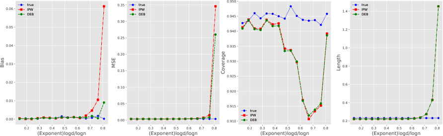
(a) $n=500$

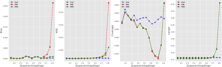
(b) $n=1000$

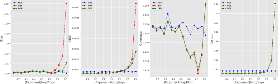
(c) $n=2000$

Figure 1: Plots of the bias, MSE, coverage, and coverage length for three different estimators $\widehat{\tau}^{\scaleto{IPW}{4pt}}_{n}$, $\widehat{\tau}^{\scaleto{DEB}{4pt}}_{n}$, $\widehat{\tau}^{\scaleto{true}{4pt}}_{n}$ in Section 4.1. For each point (on each curve in each plot), these statistics are approximated by taking a Monte Carlo average over $K=10000$ trails. Our theory predicts that $\widehat{\tau}^{\scaleto{DEB}{4pt}}_{n}$ has smaller bias and MSE than $\widehat{\tau}^{\scaleto{IPW}{4pt}}_{n}$ when $n\geq d^{0.6}$; as shown, these theoretical predictions agree well with the empirical results in the bias and MSE plots. Theory predicts that $\widehat{\tau}^{\scaleto{IPW}{4pt}}_{n}$ has bad coverage or unreasonable coverage length after $n\geq d^{0.6}$; as shown, these theoretical predictions agree well with the empirical results in the coverage and coverage length plots.

4.2 Zero-bias outcome model

In this subsection, we study a zero-bias case, where $B_{1}=B_{0}=0$. We keep the same data generating process as Section 4.1, and only change the treatment potential outcome model into

$$Y_{i}(1)=\pi^{*}(X_{i})\langle X_{i},\,(1,\ldots,1)/\sqrt{d}\rangle.$$

We have $\tau^{*}={\mathbb{E}}[Y(1)]\approx 0.1180375$.

We omit the description of similar simulation results as Section 4.1 while focus only on different one. We observe in this example that, when $d\leq n^{0.7}$, $\widehat{\tau}^{\scaleto{IPW}{4pt}}_{n}$ performs similarly as $\widehat{\tau}^{\scaleto{DEB}{4pt}}_{n}$. However, when $d$ is close to $n^{0.8}$, the bias and MSE of $\widehat{\tau}^{\scaleto{IPW}{4pt}}_{n}$ becomes larger than $\widehat{\tau}^{\scaleto{DEB}{4pt}}_{n}$. The only difference compared to Section 4.1 is that the bias and MSE of $\widehat{\tau}^{\scaleto{IPW}{4pt}}_{n}$ arise later than the one in Section 4.1. This simulation result is somewhat surprising because $\widehat{\tau}^{\scaleto{DEB}{4pt}}_{n}$ can still reduce bias and MSE compared to $\widehat{\tau}^{\scaleto{IPW}{4pt}}_{n}$ even if $B_{1}=B_{0}=0$. A conjecture is that the higher order term $H_{n}$ has positive correlation with $\widehat{B}_{1}$ and $\widehat{B}_{0}$.

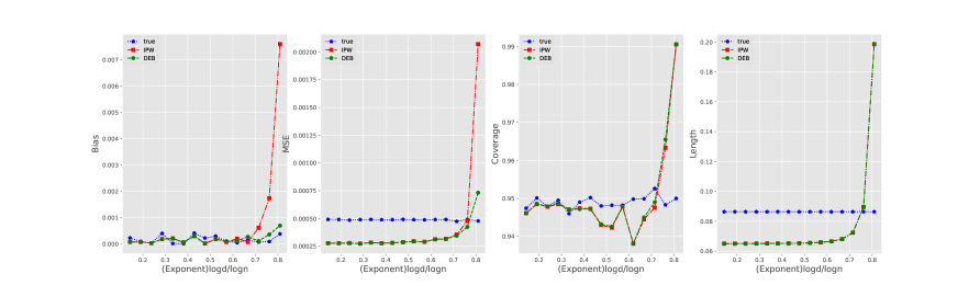
Figure 2: Simulations for the set-up of zero bias (see Section 4.2). The behavior is similar to that in Figure 1, with the main difference being that the bias and MSE of the IPW estimate $\widehat{\tau}^{\scaleto{IPW}{4pt}}_{n}$ grow at a slightly later value.

4.3 Mis-specified propensity score model

In this subsection, we study the finite sample performance of estimators under mis-specified propensity score model. We leave the theortical discussion to Section 5. Keeping the same data generating process as Section 4.1, we change propensity score model to

$$\pi^{*}(X)=(1+\exp(-\langle X,\,\beta^{*}\rangle+0.1))^{-1}.$$

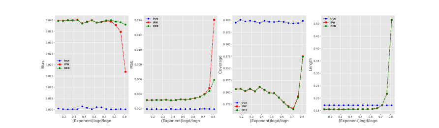
Figure 3: Simulation for a mis-specified propensity score model (see Section 4.3). As shown in the bias plot, the debiased estimator $\widehat{\tau}^{\scaleto{DEB}{4pt}}_{n}$ need not have lower bias $\widehat{\tau}^{\scaleto{IPW}{4pt}}_{n}$, and moreover, from the coverage plot, its coverage can be substantially smaller than $95\%$.

We observe that for mis-specified propensity score model, both $\widehat{\tau}^{\scaleto{IPW}{4pt}}_{n}$ and $\widehat{\tau}^{\scaleto{DEB}{4pt}}_{n}$ have large biases under both low-dimensional and high-dimensional regime. However, in this specific example and high-dimensional regime, $\widehat{\tau}^{\scaleto{DEB}{4pt}}_{n}$ has larger bias than $\widehat{\tau}^{\scaleto{IPW}{4pt}}_{n}$, but we observe that $\widehat{\tau}^{\scaleto{DEB}{4pt}}_{n}$ still has smaller MSE than $\widehat{\tau}^{\scaleto{IPW}{4pt}}_{n}$. The coverages of both $\widehat{\tau}^{\scaleto{IPW}{4pt}}_{n}$ and $\widehat{\tau}^{\scaleto{DEB}{4pt}}_{n}$ are substantially below $95\%$.

5 Discussion

In this paper, we analyze the IPW estimator based on a non-asymptotic decomposition. Using this decomposition, we show that the sample size requirement $d^{2}\lesssim n$ is necessary and sufficient for IPW estimator to be $\sqrt{n}$-consistent. Furthermore, by estimating and subtracting the leading-order bias term, we propose a debiased IPW estimator, which is $\sqrt{n}$-consistent with near-optimal variance, as long as the sample size satisfies $d^{3/2}\lesssim n$. We also establish central limit theorems and propose valid inference methodologies in the corresponding high-dimensional asymptotic regimes, for both the standard and debiased IPW estimators.

Our research opens a couple of future directions.

• First, our results are established under the well-specified logistic model. Such an assumption can be relaxed when the level of mis-specification is mild. Concretely, let us measure mis-specification via a bound of the form ${\mathbb{E}}\big{[}D_{\text{KL}}\left(\pi^{*}(X)\;\|\;\pi(X;\beta^{*})\right)\big{]}\leq\Delta^{2}$. By Pinsker’s inequality and the variational formulation of the total variation distance, the expectation of any bounded function differ by at most $\mathcal{O}\left(\Delta\right)$ under the true model $\pi^{*}$ and the best logistic approximation $\pi(\cdot;\beta^{*})$. When substituting $\pi(X;\beta^{*})$ into the IPW estimator, the mis-specified model leads to a bias of order $\mathcal{O}\left(\Delta\right)$ compared to $\tau^{*}$, in addition to the statistical errors in our current analysis. We conjecture that the analysis in Theorems 1 and 2 could be used to establish non-asymptotic guarantees for the debiased estimator under mis-specification. When applying these results to sieve logistic series, this will also lead to relaxed smoothness requirement compared to the paper [9].

• Second, while our analysis only focus on the IPW estimator for average treatment effect estimation, the techniques could apply to other popular variants, such as doubly robust estimator [23] and Hájek estimator, and more generally, a larger class of semi-parametric estimation problems with high-dimensional non-linear structures. In particular, using the $U$-statistics concentration inequalities, high-dimensional decomposition results similar to Theorem 1 could be established, leading to construction of novel debiased estimators with improved dimension dependence. (See Appendix H for a more detailed discussion of Hájek estimator.) Moreover, note that our debiasing method is to estimate the bias based on explicit formula. Jackknife, on the other hand, can automatically characterize the bias, at least in the low-dimensional regimes. Recently, the paper [6] shows that the jackknife-debiased estimator satisfies asymptotic normality if $d^{2}/n$ converges to a constant. It is an important direction of future research to further improve the dimension dependency for Jackknife methods using our approach.

• Third, though the $n\gtrsim d^{3/2}$ dimension dependency achieves the current state-of-the-art for propensity-based methods with logistic links to achieve $\sqrt{n}$-consistency in high dimensions, it is not clear whether this requirement is necessary. In particular, if we further expand the Taylor series for the IPW estimator to higher order, the structures in the high-order term $H_{n}$ in Theorem 2 could be further characterized. This strategy could potentially lead to a class of high-order debiasing methods, with further improved dimension dependency. A key open problem is about the optimal sample size threshold in terms of dimension, in order to achieve $\sqrt{n}$-consistency in ATE estimation. We conjecture that a linear dependence $n\gtrsim d$ (up to additional log factors) suffices.

  6 Proofs of Theorem 1 and Theorem 2

  We now turn to the proofs of our main results. Section 6.1 proves the decomposition of $\widehat{\tau}^{\scaleto{IPW}{4pt}}_{n}$ in Theorem 1. Section 6.2 proves the decomposition of $\widehat{\tau}^{\scaleto{DEB}{4pt}}_{n}$ in Theorem 2. The proof in Section 6 is an outline, and we leave details to Appendix A. We leave the proofs of Corollaries 1 and 2 to Appendix B.

  6.1 Proof of Theorem 1

  Recall the definition (13a) of the random variable $\bar{W}_{n}$. Our first step is subtracting a first-order Taylor series expansion of the estimator $\widehat{\tau}^{\scaleto{IPW}{4pt}}_{n}-\tau^{*}$. More precisely, we can write $\sqrt{n}\big{(}\widehat{\tau}^{\scaleto{IPW}{4pt}}_{n}-\tau^{*}\big{)}-\bar{W}_{n}=Q_{1}-Q_{0}$, where

  $$Q_{1} :=\frac{1}{\sqrt{n}}\sum_{i=1}^{n}\Big{\{}A_{i}Y_{i}\big{(}e^{-\langle X_{i},\,\widehat{\beta}_{n}\rangle}-e^{-\langle X_{i},\,\beta^{*}\rangle}\big{)}+\langle\theta_{1},\,X_{i}\rangle_{\mathbf{J}_{*}}\big{(}\pi(X_{i};\widehat{\beta}_{n})-\pi^{*}(X_{i})\big{)}\Big{\}},$$ (25a)

  $$Q_{0} :=\frac{1}{\sqrt{n}}\sum_{i=1}^{n}\Big{\{}(1-A_{i})Y_{i}\big{(}e^{\langle X_{i},\,\widehat{\beta}_{n}\rangle}-e^{\langle X_{i},\,\beta^{*}\rangle}\big{)}+\langle\theta_{0},\,X_{i}\rangle_{\mathbf{J}_{*}}\big{(}\pi^{*}(X_{i})-\pi(X_{i};\widehat{\beta}_{n})\big{)}\Big{\}}.$$ (25b)

  By symmetry, it suffices to analyze the term $Q_{1}$; results for term $Q_{0}$ can be obtained by switching the role of treated and untreated.

  We now apply a second-order Taylor series expansion with Lagrangian remainder to write $Q_{1}/\sqrt{n}=T_{1}+T_{2}+R_{1}+R_{2}$, with the first-order term

  $$T_{1}:=n^{-1}\sum_{i=1}^{n}\Big{\{}A_{i}Y_{i}e^{-\langle X_{i},\,\beta^{*}\rangle}\big{(}-\langle X_{i},\,\widehat{\beta}_{n}-\beta^{*}\rangle\big{)}+\langle\theta_{1},\,X_{i}\rangle_{\mathbf{J}_{*}}\frac{e^{\langle X_{i},\,\beta^{*}\rangle}}{(1+e^{\langle X_{i},\,\beta^{*}\rangle})^{2}}\langle X_{i},\,\widehat{\beta}_{n}-\beta^{*}\rangle\Big{\}},$$

  the second-order term

  $$T_{2}:=\frac{1}{2n}\sum_{i=1}^{n}\Big{\{}A_{i}Y_{i}e^{-\langle X_{i},\,\beta^{*}\rangle}\langle X_{i},\,\widehat{\beta}_{n}-\beta^{*}\rangle^{2}+\langle\theta_{1},\,X_{i}\rangle_{\mathbf{J}_{*}}\frac{e^{\langle X_{i},\,\beta^{*}\rangle}(1-e^{\langle X_{i},\,\beta^{*}\rangle})}{(1+e^{\langle X_{i},\,\beta^{*}\rangle})^{3}}\langle X_{i},\,\widehat{\beta}_{n}-\beta^{*}\rangle^{2}\Big{\}},$$

  and the remainder terms

  $$R_{1} :=-\frac{1}{6n}\sum_{i=1}^{n}A_{i}Y_{i}e^{-\langle X_{i},\,\widetilde{\beta}\rangle}\langle X_{i},\,\widehat{\beta}_{n}-\beta^{*}\rangle^{3},$$

  $$R_{2} :=\frac{1}{6n}\sum_{i=1}^{n}\langle\theta_{1},\,X_{i}\rangle_{\mathbf{J}_{*}}\frac{e^{\langle X_{i},\,\widetilde{\beta}\rangle}-4e^{2\langle X_{i},\,\widetilde{\beta}\rangle}+e^{3\langle X_{i},\,\widetilde{\beta}\rangle}}{(1+e^{\langle X_{i},\,\widetilde{\beta}\rangle})^{4}}\langle X_{i},\,\widehat{\beta}_{n}-\beta^{*}\rangle^{3},$$

  where $\widetilde{\beta}$ lies on the line segment between $\widehat{\beta}_{n}$ and $\beta^{*}$. The remainder terms are of higher order and can be controlled by bounding the estimation error $\|\widehat{\beta}_{n}-\beta^{*}\|_{2}$. In order to study the terms $T_{1}$ and $T_{2}$, we use a locally linear approximation of the logistic regression problem (5a). By approximating the error vector $\widehat{\beta}_{n}-\beta^{*}$ using an $\mathrm{i.i.d.}$ sum, we turn $T_{1}$ and $T_{2}$ into a particular form of degenerate $U$-statistics, the concentration behavior of which is well-understood.

  In more detail, we first define the random vectors

  $$\psi_{n}:=n^{-1}\sum_{i=1}^{n}\mathbf{J}_{*}^{-1}X_{i}(A_{i}-\pi^{*}(X_{i})),\quad\mbox{and}\quad\zeta_{n}=\widehat{\beta}_{n}-\beta^{*}-\psi_{n}.$$ (26)

  Note that $\psi_{n}$ is an empirical average of $\mathrm{i.i.d.}$ zero-mean random vectors, and the vector $\zeta_{n}$ is the higher-order approximation error.

  We can write $T_{1}=\langle q_{n},\,\psi_{n}+\zeta_{n}\rangle$, where

  $$q_{n} :=\frac{1}{n}\sum_{i=1}^{n}\Big{(}-A_{i}Y_{i}\frac{1-\pi^{*}(X_{i})}{\pi^{*}(X_{i})}+\langle\theta_{1},\,X_{i}\rangle_{\mathbf{J}_{*}}\pi^{*}(X_{i})(1-\pi^{*}(X_{i}))\Big{)}X_{i}.$$

  We can write the second-order term as $T_{2}=(\psi_{n}+\zeta_{n})^{\top}\big{\{}\mathbf{C}_{n}+\mathbf{D}_{n}\big{\}}(\psi_{n}+\zeta_{n})$, where

  $$\mathbf{C}_{n}:=\frac{1}{2n}\sum_{i=1}^{n}A_{i}Y_{i}e^{-\langle X_{i},\,\beta^{*}\rangle}X_{i}X_{i}^{\top},\quad\mbox{and}\quad\mathbf{D}_{n}:=\frac{1}{2n}\sum_{i=1}^{n}\langle\theta_{1},\,X_{i}\rangle_{\mathbf{J}_{*}}\frac{e^{\langle X_{i},\,\beta^{*}\rangle}(1-e^{\langle X_{i},\,\beta^{*}\rangle})}{(1+e^{\langle X_{i},\,\beta^{*}\rangle})^{3}}X_{i}X_{i}^{\top}.$$

  Define $\mathbf{M}_{n}:=\mathbf{C}_{n}+\mathbf{D}_{n}$, with expectation

  $$\mathbf{M} :={\mathbb{E}}[\mathbf{M}_{n}]=\frac{1}{2}{\mathbb{E}}\Big{[}\Big{\{}\mu^{*}(X,1)+\langle\theta_{1},\,X_{i}\rangle_{\mathbf{J}_{*}}\cdot\pi^{*}(X)(1-2\pi^{*}(X))\Big{\}}\big{(}1-\pi^{*}(X)\big{)}XX^{\top}\Big{]}.$$ (27)

  We have $\mathbf{M}_{n}$ concentrates around its expectation and leave the proof to Lemma 7. We decompose the term $Q_{1}$ into the sum of a $U$-statistic along with some higher-order error terms. We have

  $$T_{1}+T_{2}=\underbrace{\langle q_{n},\,\psi_{n}\rangle+\psi_{n}^{\top}\mathbf{M}\psi_{n}}_{=:U_{1,n}/\sqrt{n}}+\underbrace{\langle q_{n},\,\zeta_{n}\rangle+\psi_{n}^{\top}(\mathbf{M}_{n}-\mathbf{M})\psi_{n}+\zeta_{n}^{\top}\mathbf{M}_{n}\zeta_{n}+2\psi_{n}^{\top}\mathbf{M}_{n}\zeta_{n}}_{=:T_{3}}.$$ (28)

  Define $H_{1,n}^{(U)}:=U_{1,n}-{\mathbb{E}}[U_{1,n}]$ and $H_{1,n}^{(r)}:=\sqrt{n}(R_{1}+R_{2}+T_{3})$. We have

  $$Q_{1}=\sqrt{n}(T_{1}+T_{2}+R_{1}+R_{2})=\sqrt{n}(U_{1,n}/\sqrt{n}+T_{3}+R_{1}+R_{2})={\mathbb{E}}[U_{1,n}]+H_{1,n}^{(U)}+H_{1,n}^{(r)}.$$ (29)

  We can similarly define the terms $U_{0,n},H_{0,n}^{(U)},H_{0,n}^{(r)}$ for the untreated group (by exchanging the role of $\pi^{*}$ and $1-\pi^{*}$), which leads to the following decomposition for the term $Q_{0}$:

  $$Q_{0}={\mathbb{E}}[U_{0,n}]+H_{0,n}^{(U)}+H_{0,n}^{(r)}.$$ (30)

  We can then define the following error terms in the main decomposition result:

  $$H_{n}^{(U)}=H_{1,n}^{(U)}-H_{0,n}^{(U)},\quad\mbox{and}\quad H_{n}^{(r)}=H_{1,n}^{(r)}-H_{0,n}^{(r)}.$$

  We claim that given the sample size requirement (14), with probability $1-\delta$, for $a=0$ and $1$, we have

  $$\sqrt{n}{\mathbb{E}}[U_{a,n}] =B_{a},$$ (31a)

  $$|H_{a,n}^{(U)}| \leq\Big{(}\frac{\nu^{4}}{\gamma^{2}}+\frac{\nu}{\sqrt{\pi_{\min}\gamma}}\Big{)}\frac{c\sqrt{d}}{\sqrt{n}}\log^{2}(n/\delta),$$ (31b)

  $$|H_{a,n}^{(r)}| \leq\frac{c\nu^{10}}{\gamma^{5}\pi_{\min}}\log^{2}(n/\delta)\cdot\Big{\{}\frac{d^{3/2}}{n}+\frac{d^{3}}{n^{2}}\Big{\}}.$$ (31c)

  Finally, collecting together equations (25), (30) and (31) completes the proof.

  It remains to prove the three inequalities (31)(a)–(c), and we do so in Sections A.1, A.2 and A.3, respectively.

  6.2 Proof of Theorem 2

  To prove Theorem 2, we need Lemma 1, which guarantees non-asymptotic rates for estimating relevant quantities in constructing $\widehat{B}_{0}$ and $\widehat{B}_{1}$. Define the shorthand notation

  $$\omega:=\sqrt{\frac{d+\log(1/\delta)}{n}}.$$ (32)

  Lemma 1.

  Given a sample size lower bound (36), with probability at least $1-\delta$, we have

  $$\|\widehat{}\theta_{1}-\theta_{1}\|_{2} \leq c\frac{\nu^{3}}{\pi_{\min}\gamma}\omega\sqrt{\log(n/\delta)},\quad\|\widehat{\theta}_{1}\|_{2}\leq\frac{\nu^{3}}{\pi_{\min}\gamma},$$ (33a)

  $$|\!|\!|\widehat{\mathbf{J}}^{-1}-\mathbf{J}_{*}^{-1}|\!|\!|_{{\tiny{\textup{\mbox{op}}}}} \leq c\frac{\nu^{4}}{\gamma^{3}}\Big{[}\omega+\omega^{3}(\sqrt{n}\omega)\log^{3/2}n\Big{]},\quad|\!|\!|\widehat{\mathbf{J}}^{-1}|\!|\!|_{{\tiny{\textup{\mbox{op}}}}}\leq\frac{2}{\gamma},$$ (33b)

  $$\|\widehat{\mathbf{J}}^{-1}\widehat{\theta}_{1}-\mathbf{J}_{*}^{-1}\theta_{1}\|_{2} \leq c\frac{\nu^{7}}{\pi_{\min}\gamma^{4}}\Big{[}\omega+\omega^{3}(\sqrt{n}\omega)\log^{3/2}n\Big{]}\sqrt{\log(n/\delta)}.$$ (33c)

  See Section A.6 for the proof of this lemma. Taking it as given, we proceed with the proof of Theorem 2. Define

  $$\widehat{B}_{1}^{(\mu)} :=\frac{1}{n}\sum_{i=1}^{n}Y_{i}A_{i}\frac{(1-\pi(X_{i};\widehat{\beta}_{n}))(2\pi(X_{i};\widehat{\beta}_{n})-1)}{\pi(X_{i};\widehat{\beta}_{n})}X_{i}^{\top}\widehat{\mathbf{J}}^{-1}X_{i},$$

  $$\widehat{B}_{1}^{(cr)} :=\frac{1}{2n}\sum_{i=1}^{n}\widehat{\theta}_{1}^{\top}\widehat{\mathbf{J}}^{-1}X_{i}\pi(X_{i};\widehat{\beta}_{n})(1-\pi(X_{i};\widehat{\beta}_{n}))(1-2\pi(X_{i};\widehat{\beta}_{n}))X_{i}^{\top}\widehat{\mathbf{J}}^{-1}X_{i}.$$

  Similarly, define

  $$\widehat{B}_{0}^{(\mu)} :=\frac{1}{n}\sum_{i=1}^{n}Y_{i}(1-A_{i})\frac{\pi(X_{i};\widehat{\beta}_{n})(1-2\pi(X_{i};\widehat{\beta}_{n}))}{1-\pi(X_{i};\widehat{\beta}_{n})}X_{i}^{\top}\widehat{\mathbf{J}}^{-1}X_{i},$$

  $$\widehat{B}_{0}^{(cr)} :=\frac{1}{2n}\sum_{i=1}^{n}\widehat{\theta}_{0}^{\top}\widehat{\mathbf{J}}^{-1}X_{i}\pi(X_{i};\widehat{\beta}_{n})(1-\pi(X_{i};\widehat{\beta}_{n}))(2\pi(X_{i};\widehat{\beta}_{n})-1)X_{i}^{\top}\widehat{\mathbf{J}}^{-1}X_{i}.$$

  Then $\widehat{B}_{1}=\widehat{B}_{1}^{(\mu)}+\widehat{B}_{1}^{(cr)}$ and $\widehat{B}_{0}=\widehat{B}_{0}^{(\mu)}+\widehat{B}_{0}^{(cr)}$. Now define

  $$B_{1}^{(\mu)} :=\frac{1}{2}{\mathbb{E}}\Big{[}\mu^{*}(X,1)(1-\pi^{*}(X))\big{(}2\pi^{*}(X)-1\big{)}\cdot\|X\|_{\mathbf{J}_{*}}^{2}\Big{]},$$

  $$B_{1}^{(cr)} :=\frac{1}{2}{\mathbb{E}}\Big{[}\langle\theta_{1},\,X\rangle_{\mathbf{J}_{*}}\pi^{*}(X)(1-\pi^{*}(X))\big{(}1-2\pi^{*}(X)\big{)}\cdot\|X\|_{\mathbf{J}_{*}}^{2}\Big{]},$$

  $$B_{0}^{(\mu)} :=\frac{1}{2}{\mathbb{E}}\Big{[}\mu^{*}(X,0)\pi^{*}(X)\big{(}1-2\pi^{*}(X)\big{)}\cdot\|X\|_{\mathbf{J}_{*}}^{2}\Big{]},$$

  $$B_{0}^{(cr)} :=\frac{1}{2}{\mathbb{E}}\Big{[}(1-\pi^{*}(X))\langle\theta_{0},\,X\rangle_{\mathbf{J}_{*}}\pi^{*}(X)\big{(}2\pi^{*}(X)-1\big{)}\cdot\|X\|_{\mathbf{J}_{*}}^{2}\Big{]}.$$

  We have $B_{1}=B_{1}^{(\mu)}+B_{1}^{(cr)},B_{0}=B_{0}^{(\mu)}+B_{0}^{(cr)}.$ We have the following two lemmas regarding the concentration of $\widehat{B}_{1}^{(cr)}$ and $\widehat{B}_{1}^{(\mu)}$.

  Lemma 2.

  Given the sample size lower bound (14), we have

  $$|\widehat{B}_{1}^{(cr)}-B_{1}^{(cr)}|\leq cd\frac{\nu^{10}}{\pi_{\min}\gamma^{5}}\Big{[}\omega+\omega^{3}(\sqrt{n}\omega)\log^{3/2}n\Big{]}{\log(n/\delta)}.$$

  Lemma 3.

  Given the sample size lower bound (14), we have

  $$|\widehat{B}_{1}^{(\mu)}-B_{1}^{(\mu)}|\leq cd\frac{\nu^{10}}{\pi_{\min}\gamma^{5}}\Big{[}\omega+\omega^{3}(\sqrt{n}\omega)\log^{3/2}n\Big{]}{\log(n/\delta)}.$$

  See Sections A.7 and A.8, respectively, for the proof of these two lemmas. Because the results for $\widehat{B}_{0}^{(cr)}-B_{0}^{(cr)}$ and $\widehat{B}_{0}^{(\mu)}-B_{0}^{(\mu)}$ follows similarly, given a sample size lower bound  (14), with probability at least $1-\delta$, we have

  $$\sqrt{n}|\widehat{E}_{n}| =|(B_{1}-B_{0})-(\widehat{B}_{1}-\widehat{B}_{0})|$$

  $$=|(B_{1}^{(\mu)}+B_{1}^{(cr)}-\widehat{B}_{1}^{(\mu)}-\widehat{B}_{1}^{(cr)})-(B_{0}^{(\mu)}+B_{0}^{(cr)}-\widehat{B}_{0}^{(\mu)}-\widehat{B}_{0}^{(cr)})|$$

  $$\leq\frac{cd\nu^{10}}{\pi_{\min}\gamma^{5}}\Big{[}\omega+\omega^{3}(\sqrt{n}\omega)\log^{3/2}n\Big{]}{\log(n/\delta)}$$

  $$\leq\frac{cd\nu^{10}}{\pi_{\min}\gamma^{5}}\Big{[}\frac{\sqrt{d}+\sqrt{\log(1/\delta)}}{\sqrt{n}}+\frac{d^{2}\log^{3/2}n+\log^{7/2}(1/\delta)}{n^{3/2}}\Big{]}{\log(n/\delta)}$$

  $$\leq c\frac{\nu^{10}}{\gamma^{5}\pi_{\min}}\Big{\{}\frac{d^{3/2}}{\sqrt{}n}+\frac{d^{3}}{n^{3/2}}\Big{\}}\log^{5/2}(n/\delta).$$

Acknowledgements

This work was partially supported by NSF-DMS grant 1945136 to PD, and Office of Naval Research Grant ONR-N00014-21-1-2842, NSF-CCF grant 1955450, and NSF-DMS grant 2015454 to MJW.

Appendix

Appendix A Proofs of auxiliary lemmas used in Theorem 1 and Theorem 2

In this section, we prove the details left in Section 6. From Sections A.1, A.2, A.3, A.4 and A.5, we prove the auxiliary lemmas used in Theorem 1. From Sections A.6, A.7 and A.8, we prove the auxiliary lemmas used in Theorem 2.

A.1 Proof of $U$-statistics expectation (31a)

Recall that the observations $(X_{i},A_{i},Y_{i})_{i=1}^{n}$ are $\mathrm{i.i.d.}$, and that $A_{i}$ and $Y_{i}(1)$ are conditionally independent given $X_{i}$. Using these facts, we have

$${\mathbb{E}}[U_{1,n}] =n^{-1/2}{\mathbb{E}}\Big{\{}\Big{[}AY\frac{1-\pi^{*}(X)}{\pi^{*}(X)}(-X^{\top})\Big{]}\Big{[}\mathbf{J}_{*}^{-1}X(A-\pi^{*}(X))\Big{]}\Big{.}$$

$$\qquad+\Big{[}\theta_{1}^{\top}\mathbf{J}_{*}^{-1}X\pi^{*}(X)(1-\pi^{*}(X))X^{\top}\Big{]}\Big{[}\mathbf{J}_{*}^{-1}X(A-\pi^{*}(X))\Big{]}$$

$$\qquad\Big{.}+\Big{[}\mathbf{J}_{*}^{-1}X(A-\pi^{*}(X))\Big{]}^{\top}\mathbf{M}\Big{[}\mathbf{J}_{*}^{-1}X(A-\pi^{*}(X))\Big{]}\Big{\}}$$

$$=\frac{1}{\sqrt{n}}\Big{(}-{\mathbb{E}}[YA\frac{(1-\pi^{*}(X))^{2}}{\pi^{*}(X)}X^{\top}\mathbf{J}_{*}^{-1}X]+{\mathbb{E}}[\pi^{*}(X)(1-\pi^{*}(X))X^{\top}\mathbf{J}_{*}^{-1}\mathbf{M}\mathbf{J}_{*}^{-1}X]\Big{)}$$

$$=\frac{1}{\sqrt{n}}\Big{(}-{\mathbb{E}}[\mu^{*}(X,1)(1-\pi^{*}(X))^{2}X^{\top}\mathbf{J}_{*}^{-1}X]+\operatorname{trace}[\mathbf{M}\mathbf{J}_{*}^{-1}]\Big{)}.$$

Recall equation (27). Some algebra shows that $\sqrt{n}{\mathbb{E}}[U_{1,n}]=B_{1}$. Similarly, we have $\sqrt{n}{\mathbb{E}}[U_{0,n}]=B_{0}$, which completes the proof of equation (31a).

A.2 Proof of the U-statistic concentration bound (31b)

Note that the term $U_{1,n}$ consists of inner product of the empirical average over $n$ samples. In order to prove non-asymptotic concentration bounds on such a quantity, we make use of the following:

Lemma 4.

Given $\mathrm{i.i.d.}$ random vector pairs $(X_{i},Y_{i})_{i=1}^{n}$ such that ${\mathbb{E}}[X_{1}]={\mathbb{E}}[Y_{1}]=0$, suppose that exists scalars $v,\sigma>0$ and $\alpha\in[1,2]$ such that

$$\lambda_{\mbox{\tiny{max}}}({\mathbb{E}}[XX^{\top}]),\lambda_{\mbox{\tiny{max}}}({\mathbb{E}}[YY^{\top}])\leq v^{2},\quad\mbox{and}\quad\|\|X\|_{2}\|_{\psi_{\alpha}},\|\|Y\|_{2}\|_{\psi_{\alpha}}\leq\sigma\sqrt{d}.$$ (34)

Then for any $\delta\in(0,1)$, we have

$$\left|\langle\frac{1}{n}\sum_{i=1}^{n}X_{i},\,\frac{1}{n}\sum_{i=1}^{n}Y_{i}\rangle-\frac{1}{n}{\mathbb{E}}[\langle X,\,Y\rangle]\right|\leq\frac{cv^{2}\sqrt{d}}{n}\log(1/\delta)+\frac{c_{\alpha}\sigma^{2}d}{n^{3/2}}\log^{1/2+4/\alpha}(n/\delta)$$ (35)

with probability at least $1-\delta$.

See Appendix F for the proof of this lemma.

Note that $U_{1,n}/\sqrt{n}=\langle q_{n}+\mathbf{M}\psi_{n},\,\psi_{n}\rangle$ is an inner product between two empirical averages. Straightforward calculation yields

$${\mathbb{E}}[\psi_{n}]=0,\quad\mbox{and}\quad{\mathbb{E}}[q_{n}]=-{\mathbb{E}}[\mu^{*}(X,1)(1-\pi^{*}(X))X]+{\mathbb{E}}[\pi^{*}(X)(1-\pi^{*}(X))XX^{\top}]\mathbf{J}_{*}^{-1}\theta_{1}=0.$$

Now we study the second moment and Orlicz norms for each term in the summation $\psi_{n}$ and $q_{n}$. For $i=1,2,\ldots,n$, we define:

$$s_{i,1} =A_{i}Y_{i}\frac{1-\pi^{*}(X_{i})}{\pi^{*}(X_{i})}X_{i}-\theta_{1},$$

$$s_{i,2} =\mathbf{J}_{*}^{-1}X_{i}\{A_{i}-\pi^{*}(X_{i})\},$$

$$s_{i,3} =\left\{\pi^{*}(X_{i})(1-\pi^{*}(X_{i}))X_{i}X_{i}^{\top}\right\}\mathbf{J}_{*}^{-1}\theta_{1}-\theta_{1}.$$

We can verify that $q_{n}=\tfrac{1}{n}\sum_{i=1}^{n}(s_{i,3}-s_{i,1})$ and $\psi_{n}=\tfrac{1}{n}\sum_{i=1}^{n}s_{i,2}$.

Define $v_{j}^{2}=\lambda_{\max}({\mathbb{E}}[s_{i,j}s_{i,j}^{\top}])$ and $\sigma_{j}=d^{-1/2}\|\|s_{i,j}\|_{2}\|_{\psi_{1}}$ for $j=1,2,3$. Our analysis makes use of the following auxiliary result:

Lemma 5.

Under the setup of Theorem 1, there exists a universal constant $c>0$ such that

$$v_{1}=\frac{16\nu}{\sqrt{\pi_{\min}}},\quad v_{2}=\frac{1}{\sqrt{\gamma}},\quad v_{3}=\frac{16\nu^{3}}{\gamma},\quad\sigma_{1}\leq\frac{c\nu}{\pi_{\min}}\log(2d),\quad\sigma_{2}\leq\frac{c\nu}{\gamma}\log(2d),\quad\sigma_{3}\leq c\frac{\nu^{3}}{\gamma}\log(2d).$$

See Section A.4 for the proof of this lemma.

Recall from Lemma 7, the operator norm bound $|\!|\!|\mathbf{M}|\!|\!|_{{\tiny{\textup{\mbox{op}}}}}\leq{\nu^{4}}/{\gamma}$. Combining with Lemma 5, each term in $q_{n}+\mathbf{M}\psi_{n}$ satisfies the bound:

$$\text{for all }u\in\mathbb{S}^{d-1},\quad{\mathbb{E}}\big{[}\langle u,\,s_{i,1}-s_{i,3}+\mathbf{M}s_{i,2}\rangle^{2}\big{]}\leq 3\big{(}v_{1}^{2}+v_{3}^{2}+|\!|\!|\mathbf{M}|\!|\!|_{{\tiny{\textup{\mbox{op}}}}}^{2}v_{2}^{2}\big{)}\leq\frac{c\nu^{8}}{\gamma^{3}}+\frac{c\nu^{2}}{\pi_{\min}}=:(v^{\prime})^{2},$$

and the Orlicz norm bound:

$$\|\|s_{i,1}-s_{i,3}+\mathbf{M}s_{i,2}\|_{2}\|_{\psi_{1}}/\sqrt{d}\leq\sigma_{1}+\sigma_{3}+|\!|\!|\mathbf{M}|\!|\!|_{{\tiny{\textup{\mbox{op}}}}}\sigma_{2}\leq c\Big{(}\frac{\nu^{5}}{\gamma^{2}}+\frac{\nu}{\pi_{\min}}\Big{)}\log(2d)=:\sigma^{\prime}.$$

Applying Lemma 4 to the pair $(q_{n}+\mathbf{M}\psi_{n})/v^{\prime}$ and $\psi_{n}/v_{2}$, we have the following bound with probability $1-\delta$:

$$\frac{1}{v^{\prime}v_{2}}\Big{|}\langle q_{n}+\mathbf{M}\psi_{n},\,\psi_{n}\rangle-{\mathbb{E}}[U_{1,n}/\sqrt{n}]\Big{|}\leq\frac{c\sqrt{d}}{n}\log(1/\delta)+\frac{cd}{n^{3/2}}\Big{(}\frac{\nu^{2}}{\gamma}+\frac{1}{\pi_{\min}}\Big{)}\{\log^{2}(2d)\}\{\log^{9/2}(n/\delta)\},$$

for a universal constant $c>0$.

Given sample size satisfying the lower bound ${n}/{\log^{9}(n/\delta)}\geq\Big{(}{\nu^{2}}/{\gamma}+\pi_{\min}^{-1}\Big{)}^{2}d$, re-arranging the inequality leads to the following bound with probability $1-\delta$:

$$\left|U_{n,1}-{\mathbb{E}}[U_{n,1}]\right|\leq\Big{(}\frac{\nu^{4}}{\gamma^{2}}+\frac{\nu}{\sqrt{\pi_{\min}\gamma}}\Big{)}\frac{c\sqrt{d}}{\sqrt{n}}\log^{2}(n/\delta),$$

which completes the proof of this equation (31b).

A.3 Proof of equation (31c)

Recall that $H_{1,n}^{(r)}=\sqrt{n}(R_{1}+R_{2}+T_{3})$, and the term $T_{3}$ has the decomposition $T_{3}=\sum_{j=3}^{6}R_{j}$, where

$$R_{3}:=\frac{1}{n}\sum_{i=1}^{n}\langle-A_{i}Y_{i}e^{-\langle X_{i},\,\beta^{*}\rangle}X_{i}+\theta_{1},\,\zeta_{n}\rangle,$$

$$R_{4}:=n^{-1}\sum_{i=1}^{n}[\theta_{1}^{\top}\mathbf{J}_{*}^{-1}\{X_{i}\pi^{*}(X_{i})(1-\pi^{*}(X_{i}))X_{i}\}-\theta_{1}^{\top}]\zeta_{n},$$

$$R_{5}:=(\widehat{\beta}_{n}-\beta^{*})^{\top}(\mathbf{M}_{n}-\mathbf{M})(\widehat{\beta}_{n}-\beta^{*}),\quad$$

$$R_{6}:=2(\widehat{\beta}_{n}-\beta^{*})^{\top}\mathbf{M}\zeta_{n}-\zeta_{n}^{\top}\mathbf{M}\zeta_{n}.$$

We bound each of these terms in turn.

Our analysis relies on the following lemma, which characterizes the behavior of the maximal likelihood estimator $\widehat{\beta}_{n}$. In addition to standard convergence rates (in Euclidean distance), we also need its high-order expansion properties, as well as the projection onto individual data vectors.

To derive the property for logistic regression model, we require that the sample size $n$ satisfies the lower bound

$$\frac{n}{\log^{4}(n/\delta)} \geq c\frac{\nu^{8}}{\gamma^{4}}d^{4/3}\quad\mbox{for some universal constant $c>0$.}$$ (36)

This lower bound is weaker than the lower bound  (14) required in Theorem 1 and Theorem 2.

Lemma 6.

Under Assumptions (TC) and the sample size lower bound (36), we have

$$\|\widehat{\beta}_{n}-\beta^{*}\|_{2} \leq c\frac{\nu}{\gamma}\sqrt{\frac{d+\log(1/\delta)}{n}}$$ (37a)

with probability at least $1-\delta$. Furthermore, with probability at least $1-\delta$, the residual term $\zeta_{n}$ defined in equation (26) satisfies the bound

$$\|\zeta_{n}\|_{2}\leq c\frac{\nu^{5}(d+\log(1/\delta))}{\gamma^{3}n}\sqrt{\log(n/\delta)}$$ (37b)

Moreover, with probability at least $1-\delta$, we have

$$\max_{i=1,\ldots,n}|\langle X_{i},\,\widehat{\beta}_{n}-\beta^{*}\rangle| <1.$$ (37c)

See Appendix D for the proof of Lemma 6.

By considering the logistic model as a special case of general GLMs, equations (37a) and (37b) are consistent with Portnoy’s [17] result that we have asymptotic normality guarantees for the coefficient of GLMs when $d^{2}/n\rightarrow 0$, and also the limiting behavior $d^{2}/n\rightarrow 0$ is necessary for normal approximation. Taking Lemma 6 as given, we proceed with the proof of equation (31c). We first note from equation (37c) and Assumption (SO) that:

$$\text{for all }i\in[n]~{}\mbox{and}~{}\gamma\in[0,1],\quad e^{-1}\frac{\pi_{\min}}{1-\pi_{\min}}\leq\exp\Big{(}-\langle\gamma\beta^{*}+(1-\gamma)\widehat{\beta}_{n},\,X_{i}\rangle\Big{)}\leq e\frac{1-\pi_{\min}}{\pi_{\min}},$$ (38)

with probability $1-\delta$.

For the term $R_{1}$, equation (38) and Lemma 13 imply that, with probability at least $1-\delta$,

$$|R_{1}| =\left|\frac{1}{6n}\sum_{i=1}^{n}\Big{[}-A_{i}Y_{i}e^{-\langle X_{i},\,\widetilde{\beta}\rangle}\langle X_{i},\,\widehat{\beta}_{n}-\beta^{*}\rangle^{3}\Big{]}\right|$$

$$\leq\frac{e}{6\pi_{\min}}\|\widehat{\beta}_{n}-\beta^{*}\|_{2}^{3}\max_{v\in\mathbb{S}^{d-1}}\frac{1}{n}\sum_{i=1}^{n}|\langle X_{i},\,v\rangle|^{3}|Y_{i}|$$

$$\leq\frac{c\nu^{6}}{\pi_{\min}\gamma^{3}}\Big{(}\omega^{3}+\omega^{5}(\sqrt{n}\omega)\log^{3/2}n\Big{)}\sqrt{\log(n/\delta)}.$$

We now bound the term $R_{2}$. By equation (11a), the vector $\theta_{1}$ satisfies the bound

$$\|\mathbf{J}_{*}^{-1}\theta_{1}\|_{2}=\sup_{u\in\mathbb{S}^{d-1}}{\mathbb{E}}\big{[}(1-\pi^{*}(X))\mu^{*}(X,1)u^{\top}\mathbf{J}_{*}^{-1}X\big{]}\\ \leq\sqrt{{\mathbb{E}}[\mu^{*}(X,1)^{2}]}\cdot\sup_{u\in\mathbb{S}^{d-1}}\sqrt{u^{\top}\mathbf{J}_{*}^{-1}{\mathbb{E}}\big{[}(1-\pi^{*}(X))^{2}XX^{\top}\big{]}\mathbf{J}_{*}^{-1}u}\leq\frac{\nu}{\gamma}.$$ (39)

Moreover, the function $x\mapsto(x-4x^{2}+x^{3})/{(1+x)^{4}}$ is uniformly bounded for $x>0$. Consequently, Lemma 13 implies that, with probability at least $1-\delta$, the absolute value can be bounded as

$$|R_{2}| \leq\left|\frac{1}{6n}\sum_{i=1}^{n}\Big{[}\theta_{1}^{\top}\mathbf{J}_{*}^{-1}X_{i}\frac{e^{\langle X_{i},\,\widetilde{\beta}\rangle}-4e^{2\langle X_{i},\,\widetilde{\beta}\rangle}+e^{3\langle X_{i},\,\widetilde{\beta}\rangle}}{(1+e^{\langle X_{i},\,\widetilde{\beta}\rangle})^{4}}\langle X_{i},\,\widehat{\beta}_{n}-\beta^{*}\rangle^{3}\Big{]}\right|$$

$$\leq\frac{\nu}{\gamma}\|\widehat{\beta}_{n}-\beta^{*}\|_{2}^{3}\cdot\max_{u\in\mathbb{S}^{d-1}}\frac{1}{n}\sum_{i=1}^{n}|\langle\mathbf{J}_{*}^{-1}\theta_{1}/\|\mathbf{J}_{*}^{-1}\theta_{1}\|_{2},\,X_{i}\rangle|\cdot|\langle X_{i},\,u\rangle|^{3}$$

$$\leq\frac{c\nu^{8}}{\gamma^{4}}\Big{\{}\omega^{3}+\omega^{5}(\sqrt{n}\omega)\log^{3/2}n\Big{\}}\sqrt{\log(n/\delta)}.$$

Now Lemmas 6 and 12 in conjunction guarantee that, with probability at least $1-\delta$, we have:

$$|R_{3}| =\left|n^{-1}\sum_{i=1}^{n}\langle A_{i}Y_{i}e^{-\langle X_{i},\,\beta^{*}\rangle}(-X_{i})+\theta_{1},\,\zeta_{n}\rangle\right|$$

$$\leq\|n^{-1}\sum_{i=1}^{n}A_{i}Y_{i}e^{-\langle X_{i},\,\beta^{*}\rangle}(-X_{i})+\theta_{1}\|_{2}\cdot\|\zeta_{n}\|_{2}$$

$$\leq\frac{c}{\pi_{\min}}\Big{(}\frac{\nu^{6}}{\gamma^{3}}\Big{)}\omega^{3}\sqrt{\log(n/\delta)}.$$

Similarly, by Lemmas 6 and 12, with probability at least $1-\delta$, we have

$$|R_{4}| =\left|n^{-1}\sum_{i=1}^{n}\Big{[}\left(\theta_{1}^{\top}\mathbf{J}_{*}^{-1}\left\{X_{i}\pi^{*}(X_{i})(1-\pi^{*}(X_{i}))X_{i}^{\top}\right\}-\theta_{1}^{\top}\right)\zeta_{n}\Big{]}\right|$$

$$\leq\|\theta_{1}\|_{2}\cdot\|n^{-1}\sum_{i=1}^{n}\mathbf{J}_{*}^{-1}\left\{X_{i}\pi^{*}(X_{i})(1-\pi^{*}(X_{i}))X_{i}^{\top}\right\}-I_{d}\|_{2}\cdot\|\zeta_{n}\|_{2}$$

$$\leq\Big{(}\frac{c\nu^{8}}{\gamma^{4}}\Big{)}\omega^{3}\sqrt{\log(n/\delta)}.$$

To study the terms $R_{5}$ and $R_{6}$, we need Lemma 7, which guarantees that the random matrix $\mathbf{M}_{n}$ concentrates around its expectation:

Lemma 7.

Under Assumptions (TC)—(SO),

$$|\!|\!|\mathbf{M}_{n}-\mathbf{M}|\!|\!|_{{\tiny{\textup{\mbox{op}}}}}\leq\frac{\nu^{4}}{\gamma\pi_{\min}}\Big{(}\omega+\omega^{2}\log n\Big{)}\sqrt{\log(n/\delta)}\quad\mbox{and}\quad|\!|\!|\mathbf{M}|\!|\!|_{{\tiny{\textup{\mbox{op}}}}}\leq\frac{\nu^{4}}{2\gamma}$$

hold with probability at least $1-\delta$.

See Section A.5 for the proof. Taking it as given, we proceed with the studying of $R_{5},R_{6}$. By Lemmas 7 and 6, with probability $1-\delta$, we have

$$|R_{5}|=|(\widehat{\beta}_{n}-\beta^{*})^{\top}\Big{(}\mathbf{M}_{n}-\mathbf{M}\Big{)}(\widehat{\beta}_{n}-\beta^{*})| \leq\|\widehat{\beta}_{n}-\beta^{*}\|_{2}^{2}\cdot|\!|\!|\mathbf{M}_{n}-\mathbf{M}|\!|\!|_{{\tiny{\textup{\mbox{op}}}}}$$

$$\leq\frac{c\nu^{6}}{\gamma^{3}\pi_{\min}}\Big{(}\omega^{3}+\omega^{4}\log n\Big{)}\sqrt{\log(n/\delta)}.$$

Similarly, by Lemmas 7 and 6, we have

$$|R_{6}|=|2\zeta_{n}^{\top}\mathbf{M}(\widehat{\beta}_{n}-\beta^{*})-\zeta_{n}^{\top}\mathbf{M}\zeta_{n}| \leq 2\|\zeta_{n}\|_{2}\cdot|\!|\!|\mathbf{M}|\!|\!|_{{\tiny{\textup{\mbox{op}}}}}\cdot\|\widehat{\beta}_{n}-\beta^{*}\|_{2}+\|\zeta_{n}\|_{2}^{2}\cdot|\!|\!|\mathbf{M}|\!|\!|_{{\tiny{\textup{\mbox{op}}}}}$$

$$\leq c(\frac{\nu^{10}}{{\gamma^{5}}})\omega^{3}\sqrt{\log(n/\delta)}.$$

Collecting the above bounds, we conclude that there exists a universal constant $c>0$ such that

$$|H_{n}^{(r)}|\leq\sqrt{n}\sum_{i=1}^{6}|R_{i}| \leq c\frac{\sqrt{n}}{\pi_{\min}}(\frac{\nu^{10}}{{\gamma^{5}}})\Big{\{}\omega^{3}+\omega^{5}(\sqrt{n}\omega)\log^{3/2}n\Big{\}}\sqrt{\log(n/\delta)}$$

$$\leq c\frac{\nu^{10}}{\gamma^{5}\pi_{\min}}\Big{\{}\frac{d^{3/2}+\log(1/\delta)^{3/2}}{n}+\frac{d^{3}\log^{3/2}n+\log^{9/2}(n/\delta)}{n^{2}}\Big{\}}\sqrt{\log(n/\delta)}$$

$$\leq c\frac{\nu^{10}}{\gamma^{5}\pi_{\min}}\Big{\{}\frac{d^{3/2}}{n}+\frac{d^{3}}{n^{2}}\Big{\}}\log^{2}(n/\delta),$$

with probability $1-\delta$. We have thus established the claim (31c).

A.4 Proof of Lemma 5

For any $d$-dimensional random vector $Z$, Pisier’s inequality [16] implies that

$$\|\|Z\|_{2}\|_{\psi_{\alpha}}\leq\sqrt{d}\cdot\|\|Z\|_{\infty}\|_{\psi_{\alpha}}\leq c_{\alpha}\sqrt{d}\{\log^{1/\alpha}(2d)\}\max_{j\in[d]}\|\langle e_{j},\,Z\rangle\|_{\psi_{\alpha}},$$ (40)

for a constant $c_{\alpha}>0$ depending only on $\alpha$.

For any unit vector $u\in\mathbb{S}^{d-1}$, we have

$${\mathbb{E}}\big{[}\langle u,\,s_{i,1}\rangle^{2}\big{]}\leq{\mathbb{E}}\big{[}A^{2}Y^{2}\frac{(1-\pi^{*}(X))^{2}}{\pi^{*}(X)^{2}}\langle u,\,X\rangle^{2}\big{]}\leq\frac{1}{\pi_{\min}}\sqrt{{\mathbb{E}}[Y(1)^{4}]\cdot{\mathbb{E}}[\langle u,\,X\rangle^{4}]}\leq\frac{16\nu^{2}}{\pi_{\min}}=:v_{1}^{2}$$

and

$$\|\langle u,\,s_{i,1}\rangle\|_{\psi_{1}}\leq\frac{1}{\pi_{\min}}\|Y_{i}\|_{\psi_{2}}\cdot\|\langle u,\,X_{i}\rangle\|_{\psi_{2}}\leq\frac{\nu}{\pi_{\min}}.$$ (41)

Combining equation (41) with equation (40) yields $\|\|s_{i,1}\|_{2}\|_{\psi_{1}}\leq c{\nu\sqrt{d}}\log(2d)/{\pi_{\min}}$. Therefore, we have $\sigma_{1}\leq c{\nu}\log(2d)/{\pi_{\min}}$.

For the term $s_{i,2}$, we note that:

$$|\!|\!|{\mathbb{E}}[s_{i,2}s_{i,2}^{\top}]|\!|\!|_{{\tiny{\textup{\mbox{op}}}}}=|\!|\!|\mathbf{J}_{*}^{-1}{\mathbb{E}}\big{[}(A-\pi^{*}(X))^{2}XX^{\top}\big{]}\mathbf{J}_{*}^{-1}|\!|\!|_{{\tiny{\textup{\mbox{op}}}}}=|\!|\!|\mathbf{J}_{*}^{-1}|\!|\!|_{{\tiny{\textup{\mbox{op}}}}}\leq\frac{1}{\gamma},$$

which implies that $v_{2}=1/\sqrt{\gamma}$.

Moreover, for any unit vector $u\in\mathbb{S}^{d-1}$, we have the Orlicz norm bound $\|\langle s_{i,2},\,u\rangle\|_{\psi_{1}}\leq\|\langle\mathbf{J}_{*}^{-1}X_{i},\,u\rangle\|_{\psi_{1}}\leq{\nu}/{\gamma}$. Therefore, we have $\sigma_{2}=\|\|s_{i,2}\|_{2}\|_{\psi_{1}}/\sqrt{d}\leq c\nu\log(2d)/\gamma$. Now we consider the term $s_{i,3}$. By inequality (39) from Section A.3, for any unit vector $u\in\mathbb{S}^{d-1}$, we have

$${\mathbb{E}}[\langle u,\,s_{i,3}\rangle^{2}]\leq{\mathbb{E}}\big{[}\pi^{*}(X)^{2}(1-\pi^{*}(X))^{2}\langle u,\,X\rangle^{2}(\theta_{1}^{\top}\mathbf{J}_{*}^{-1}X)^{2}\big{]}\leq\sqrt{{\mathbb{E}}[\langle u,\,X\rangle^{4}]}\cdot\sqrt{{\mathbb{E}}[(\theta_{1}^{\top}\mathbf{J}_{*}^{-1}X)^{4}]}\leq\frac{16\nu^{6}}{\gamma^{2}}:=v_{3}^{2}$$

and

$$\|\langle u,\,s_{i,3}\rangle\|_{\psi_{1}}\leq\|\langle u,\,X_{i}\rangle\|_{\psi_{2}}\cdot\|\theta_{1}\mathbf{J}_{*}^{-1}X_{i}\|_{\psi_{2}}\leq\frac{\nu^{3}}{\gamma}.$$

Therefore, we have $\sigma_{3}\leq c\frac{\nu^{3}}{\gamma}\log(2d)$.

A.5 Proof of Lemma 7

Since $\mathbf{M}_{n}=\mathbf{C}_{n}+\mathbf{D}_{n}$, we split our analysis into two parts. Define $\mathbf{C}={\mathbb{E}}[\mathbf{C}_{n}]$ and $\mathbf{D}:={\mathbb{E}}[\mathbf{D}_{n}]$.

Analysis of $\mathbf{C}_{n}$:

Beginning with the definition of $\mathbf{C}_{n}$, we have

$$|\!|\!|\mathbf{C}_{n}-\mathbf{C}|\!|\!|_{{\tiny{\textup{\mbox{op}}}}}=\frac{1}{2}\max_{u\in\mathbb{S}^{d-1}}\Big{|}\frac{1}{n}\sum_{i=1}^{n}A_{i}Y_{i}\frac{1-\pi^{*}(X_{i})}{\pi^{*}(X_{i})}\langle X_{i},\,u\rangle^{2}-{\mathbb{E}}\Big{[}AY\frac{1-\pi^{*}(X)}{\pi^{*}(X)}\langle X,\,u\rangle^{2}\Big{]}\Big{|}.$$

Using the sub-Gaussian conditions in Assumption (TC), we can apply Lemma 12 to obtain that

$$|\!|\!|\mathbf{C}_{n}-\mathbf{C}|\!|\!|_{{\tiny{\textup{\mbox{op}}}}}\leq\frac{c\nu^{2}}{\pi_{\min}}\Big{(}\omega+\omega^{2}\log n\Big{)}\sqrt{\log(n/\delta)}\quad\mbox{with probability at least $1-\delta$.}$$

Furthermore, we have the upper bound

$$|\!|\!|\mathbf{C}|\!|\!|_{{\tiny{\textup{\mbox{op}}}}}\leq\frac{1}{2}\max_{u\in\mathbb{S}^{d-1}}{\mathbb{E}}\Big{[}Y(1)(1-\pi^{*}(X))\,\langle X,\,u\rangle^{2}\Big{]}\leq\frac{\nu^{2}}{2}.$$

Analysis of $\mathbf{D}_{n}$:

First, recall from inequality (39) from Section A.3, we note that

$$\|\mathbf{J}_{*}^{-1}\theta_{1}\|_{2}\leq\frac{\nu}{\gamma}.$$

For each fixed vector $u\in\mathbb{S}^{d-1}$, the random variables $\langle X,\,u\rangle$ and $\langle\theta_{1},\,X\rangle_{\mathbf{J}_{*}}$ are sub-Gaussian with Orlicz $\psi_{2}$-norms $\nu$ and $\nu^{2}/\gamma$, respectively. Lemma 12 guarantees that

$$|\!|\!|\mathbf{D}_{n}-\mathbf{D}|\!|\!|_{{\tiny{\textup{\mbox{op}}}}} =\max_{u\in\mathbb{S}^{d-1}}\Big{|}\frac{1}{2n}\sum_{i=1}^{n}\langle\theta_{1},\,X_{i}\rangle_{\mathbf{J}_{*}}\pi^{*}(X_{i})(1-\pi^{*}(X_{i}))(1-2\pi^{*}(X_{i}))\langle X_{i},\,u\rangle^{2}$$

$$\qquad-{\mathbb{E}}\Big{[}\frac{1}{2n}\sum_{i=1}^{n}\langle\theta_{1},\,X\rangle_{\mathbf{J}_{*}}\pi^{*}(X)(1-\pi^{*}(X))(1-2\pi^{*}(X))\langle X,\,u\rangle^{2}\Big{]}\Big{|}$$

$$\leq\frac{c\nu^{4}}{\gamma}\Big{(}\omega+\omega^{2}\log n\Big{)}\sqrt{\log(n/\delta)}$$

with probability at least $1-\delta$. Moreover, we have the population-level operator norm bound

$$|\!|\!|\mathbf{D}|\!|\!|_{{\tiny{\textup{\mbox{op}}}}}=\max_{u\in\mathbb{S}^{d-1}}\frac{1}{2}{\mathbb{E}}\Big{\{}\langle\theta_{1},\,X\rangle_{\mathbf{J}_{*}}\pi^{*}(X)\;(1-\pi^{*}(X))(1-2\pi^{*}(X))\langle X,\,u\rangle^{2}\Big{\}} \leq\frac{\nu^{4}}{2\gamma}$$ (42)

Collecting above bounds completes the proof of Lemma 7.

A.6 Proof of Lemma 1

We start with the error decomposition $\widehat{}\theta_{1}-\theta_{1}=R_{\theta,1}+R_{\theta,2}$, where

$$R_{\theta,1} :=n^{-1}\sum_{i=1}^{n}A_{i}Y_{i}\frac{1-\pi(X_{i};\widehat{\beta}_{n})}{\pi(X_{i};\widehat{\beta}_{n})}X_{i}-n^{-1}\sum_{i=1}^{n}A_{i}Y_{i}\frac{1-\pi^{*}(X_{i})}{\pi^{*}(X_{i})}X_{i},$$

$$R_{\theta,2} :=n^{-1}\sum_{i=1}^{n}A_{i}Y_{i}\frac{1-\pi^{*}(X_{i})}{\pi^{*}(X_{i})}X_{i}-{\mathbb{E}}\Big{[}AY\frac{1-\pi^{*}(X)}{\pi^{*}(X)}X\Big{]}.$$

Using the mean-value theorem, we write

$$\|R_{\theta,1}\|_{2} =\|n^{-1}\sum_{i=1}^{n}A_{i}Y_{i}\int_{0}^{1}e^{-\langle X_{i},\,(1-t)\beta^{*}+t\widehat{\beta}_{n}\rangle}dtX_{i}X_{i}^{\top}(\widehat{\beta}_{n}-\beta^{*})\|_{2}$$

$$\leq|\!|\!|n^{-1}\sum_{i=1}^{n}A_{i}Y_{i}\int_{0}^{1}e^{-\langle X_{i},\,(1-t)\beta^{*}+t\widehat{\beta}_{n}\rangle}dtX_{i}X_{i}^{\top}|\!|\!|_{{\tiny{\textup{\mbox{op}}}}}\|\widehat{\beta}_{n}-\beta^{*}\|_{2}.$$

Define the event

$$\mathscr{E}:=\Big{\{}\mbox{equations~{}\eqref{eq:betahat-rate-of-convergence}--\eqref{eq:logistic-regression-project-to-data} hold}\Big{\}},$$

and observe that by Lemma 6, we have ${\mathbb{P}}(\mathscr{E})\geq 1-\delta$ whenever the sample size satisfies (36). On the event $\mathscr{E}$, we have the upper bound

$$\|R_{\theta,1}\|_{2}\leq\frac{c\nu\omega}{\gamma\pi_{\min}}\cdot\sup_{u,v\in\mathbb{S}^{d-1}}n^{-1}\sum_{i=1}^{n}Y_{i}\left|\langle X_{i},\,u\rangle\right|\cdot\left|\langle X_{i},\,v\rangle\right|.$$

Applying Lemma 13 guarantees that

$$\|R_{\theta,1}\|_{2}\leq c\frac{\nu^{2}}{\pi_{\min}}(1+\omega+\omega^{2}\log n)\sqrt{\log(n/\delta)}\frac{\nu}{\gamma}\omega\leq c\frac{\nu^{3}\omega}{\pi_{\min}\gamma}\sqrt{\log(n/\delta)}.$$

with probability at least $1-\delta$. Moreover, by Lemma 12, we have

$$\|R_{\theta,2}\|_{2}\leq c\frac{\nu}{\pi_{\min}}(\omega+\omega^{2}\log n).$$

Putting together these bounds yields

$$\|\widehat{}\theta_{1}-\theta_{1}\|_{2}\leq c\frac{\nu^{3}}{\pi_{\min}\gamma}\omega\sqrt{\log(n/\delta)}.$$

Since $\|\theta_{1}\|_{2}\leq\nu$, we have established the claim (33a).

Next we analyze the estimate $\widehat{\mathbf{J}}$. Define $\beta(s)=\beta^{*}+s(\widehat{\beta}_{n}-\beta^{*})$. By Lemma 13, with probability $1-\delta$, we have

$$|\!|\!|\widehat{\mathbf{J}}-\mathbf{J}_{*}|\!|\!|_{{\tiny{\textup{\mbox{op}}}}} \leq|\!|\!|\frac{1}{n}\sum_{i=1}^{n}X_{i}X_{i}^{\top}\int_{0}^{1}\frac{e^{\langle X_{i},\,\beta(s)\rangle}(1-e^{\langle X_{i},\,\beta(s)\rangle})}{(1+e^{\langle X_{i},\,\beta(s)\rangle})^{3}}ds\langle X_{i},\,\widehat{\beta}_{n}-\beta^{*}\rangle|\!|\!|_{{\tiny{\textup{\mbox{op}}}}}+|\!|\!|\mathbf{J}_{n}(\beta^{*})-\mathbf{J}_{*}|\!|\!|_{{\tiny{\textup{\mbox{op}}}}}$$

$$\leq\max_{u\in\mathbb{S}^{d-1}}\max_{v\in\mathbb{S}^{d-1}}\frac{1}{n}\sum_{i=1}^{n}\langle X_{i},\,u\rangle^{2}|\langle X_{i},\,v\rangle|\cdot\|\widehat{\beta}_{n}-\beta^{*}\|_{2}+|\!|\!|\mathbf{J}_{n}(\beta^{*})-\mathbf{J}_{*}|\!|\!|_{{\tiny{\textup{\mbox{op}}}}}$$

$$\leq c\frac{\nu^{4}}{\gamma}\Big{[}\omega+\omega^{3}(\sqrt{n}\omega)\log^{3/2}n\Big{]}.$$ (43)

Under the sample size lower bound (36), we have

$$\omega+\omega^{3}(\sqrt{n}\omega)\log^{3/2}(n)=\sqrt{\frac{d+\log(1/\delta)}{n}}+\frac{(d+\log(1/\delta))^{2}\log^{3/2}n}{n\sqrt{n}}\leq\frac{\gamma^{2}}{2\nu^{4}}.$$ (44)

Therefore, by equations (43) and (44), we have $|\!|\!|\widehat{\mathbf{J}}-\mathbf{J}_{*}|\!|\!|_{{\tiny{\textup{\mbox{op}}}}}\leq\frac{\gamma}{2}$. By Proposition E.1 in the paper [13], we have

$$|\!|\!|\widehat{\mathbf{J}}^{-1}-\mathbf{J}_{*}^{-1}|\!|\!|_{{\tiny{\textup{\mbox{op}}}}} \leq\frac{|\!|\!|\mathbf{J}_{*}^{-1}|\!|\!|_{{\tiny{\textup{\mbox{op}}}}}^{2}|\!|\!|\widehat{\mathbf{J}}-\mathbf{J}_{*}|\!|\!|_{{\tiny{\textup{\mbox{op}}}}}}{1-\min\{1,|\!|\!|\mathbf{J}_{*}^{-1}|\!|\!|_{{\tiny{\textup{\mbox{op}}}}}|\!|\!|\widehat{\mathbf{J}}-\mathbf{J}_{*}|\!|\!|_{{\tiny{\textup{\mbox{op}}}}}\}}$$

$$\leq\frac{\gamma^{-2}|\!|\!|\widehat{\mathbf{J}}-\mathbf{J}_{*}|\!|\!|_{{\tiny{\textup{\mbox{op}}}}}}{1-\min\{1,\gamma^{-1}\frac{\gamma}{2}\}}\leq c\frac{\nu^{4}}{\gamma^{3}}\Big{[}\omega+\omega^{3}(\sqrt{n}\omega)\log^{3/2}n\Big{]}.$$

Inequality (44) implies that $|\!|\!|\widehat{\mathbf{J}}^{-1}|\!|\!|_{{\tiny{\textup{\mbox{op}}}}}\leq|\!|\!|\mathbf{J}_{*}^{-1}|\!|\!|_{{\tiny{\textup{\mbox{op}}}}}+|\!|\!|\widehat{\mathbf{J}}^{-1}-\mathbf{J}_{*}^{-1}|\!|\!|_{{\tiny{\textup{\mbox{op}}}}}\leq 2\gamma^{-1}$, so that we established inequality (33b). Finally, by inequalities (33a) and (33b), we have

$$\|\widehat{\mathbf{J}}^{-1}\widehat{\theta}_{1}-\mathbf{J}_{*}^{-1}\theta_{1}\|_{2} \leq\|(\widehat{\mathbf{J}}^{-1}-\mathbf{J}_{*}^{-1})\theta_{1}\|_{2}+\|\mathbf{J}_{*}^{-1}(\widehat{\theta}_{1}-\theta_{1})\|_{2}+\|(\widehat{\mathbf{J}}^{-1}-\mathbf{J}_{*}^{-1})(\widehat{\theta}_{1}-\theta_{1})\|_{2}$$

$$\leq c|\!|\!|\widehat{\mathbf{J}}^{-1}-\mathbf{J}_{*}^{-1}|\!|\!|_{{\tiny{\textup{\mbox{op}}}}}(\|\theta_{1}\|_{2}+\|\widehat{\theta}_{1}\|_{2})+|\!|\!|\mathbf{J}_{*}^{-1}|\!|\!|_{{\tiny{\textup{\mbox{op}}}}}\|\widehat{\theta}_{1}-\theta_{1}\|_{2}$$

$$\leq c\frac{\nu^{7}}{\pi_{\min}\gamma^{4}}\Big{[}\omega+\omega^{3}(\sqrt{n}\omega)\log^{3/2}n\Big{]}\sqrt{\log(n/\delta)},$$

which completes the proof of inequality (33c).

A.7 Proof of Lemma 2

Recall that

$$\widehat{B}_{1}^{(cr)}=\frac{1}{2n}\sum_{i=1}^{n}\widehat{\theta}_{1}^{\top}\widehat{\mathbf{J}}^{-1}X_{i}\pi(X_{i};\widehat{\beta}_{n})(1-\pi(X_{i};\widehat{\beta}_{n}))(1-2\pi(X_{i};\widehat{\beta}_{n}))(X_{i}^{\top}\widehat{\mathbf{J}}^{-1}X_{i}).$$

We decompose the difference as $2(\widehat{B}_{1}^{(cr)}-B_{1}^{(cr)})=R_{1}^{(cr)}+R_{2}^{(cr)}+R_{3}^{(cr)}+R_{4}^{(cr)}$, where

$$R_{1}^{(cr)} :=\frac{1}{n}\sum_{i=1}^{n}\{(\widehat{\theta}_{1}^{\top}\widehat{\mathbf{J}}^{-1}-\theta_{1}^{\top}\mathbf{J}_{*}^{-1})X_{i}\}\pi(X_{i};\widehat{\beta}_{n})(1-\pi(X_{i};\widehat{\beta}_{n}))(1-2\pi(X_{i};\widehat{\beta}_{n}))(X_{i}^{\top}\widehat{\mathbf{J}}^{-1}X_{i}),$$

$$R_{2}^{(cr)} :=\frac{1}{n}\sum_{i=1}^{n}(\theta_{1}^{\top}\mathbf{J}_{*}^{-1}X_{i})\pi(X_{i};\widehat{\beta}_{n})(1-\pi(X_{i};\widehat{\beta}_{n}))(1-2\pi(X_{i};\widehat{\beta}_{n}))\{X_{i}^{\top}(\widehat{\mathbf{J}}^{-1}-\mathbf{J}_{*}^{-1})X_{i}\},$$

$$R_{4}^{(cr)} :=\frac{1}{n}\sum_{i=1}^{n}(\theta_{1}^{\top}\mathbf{J}_{*}^{-1}X_{i})\pi^{*}(X_{i})(1-\pi^{*}(X_{i}))(1-2\pi^{*}(X_{i}))(X_{i}^{\top}\mathbf{J}_{*}^{-1}X_{i})-2B_{1}^{(cr)},$$

and

$$R_{3}^{(cr)}:=\frac{1}{n}\sum_{i=1}^{n}(\theta_{1}^{\top}\mathbf{J}_{*}^{-1}X_{i})\Big{\{}\pi(X_{i};\widehat{\beta}_{n})(1-\pi(X_{i};\widehat{\beta}_{n}))(1-2\pi(X_{i};\widehat{\beta}_{n}))\\ -\pi^{*}(X_{i})(1-\pi^{*}(X_{i}))(1-2\pi^{*}(X_{i}))\Big{\}}(X_{i}^{\top}\mathbf{J}_{*}^{-1}X_{i}).$$

Define $v_{1}:=(\widehat{\mathbf{J}}^{-1}\widehat{\theta}_{1}-\mathbf{J}_{*}^{-1}\theta_{1})/\|\widehat{\mathbf{J}}^{-1}\widehat{\theta}_{1}-\mathbf{J}_{*}^{-1}\theta_{1}\|_{2}$. By Lemmas 1 and 13, with probability $1-\delta$, we have

$$\begin{aligned} |R_{1}^{(cr)}|&\leq d|\!|\!|\frac{1}{n}\sum_{i=1}^{n}\{(\widehat{\theta}_{1}^{\top}\widehat{\mathbf{J}}^{-1}-\theta_{1}^{\top}\mathbf{J}_{*}^{-1})X_{i}\}\pi(X_{i};\widehat{\beta}_{n})(1-\pi(X_{i};\widehat{\beta}_{n}))(1-2\pi(X_{i};\widehat{\beta}_{n}))\widehat{\mathbf{J}}^{-1}X_{i}X_{i}^{\top}|\!|\!|_{{\tiny{\textup{\mbox{op}}}}}\\ &\leq\frac{d}{\gamma}\|\widehat{\theta}_{1}^{\top}\widehat{\mathbf{J}}^{-1}-\theta_{1}^{\top}\mathbf{J}_{*}^{-1}\|_{2}\max_{u\in\mathbb{S}^{d-1}}\frac{1}{n}\sum_{i=1}^{n}\left|\langle X_{i},\,v_{1}\rangle\right|\langle X_{i},\,u\rangle^{2}\\ &\leq c(\frac{d\nu^{10}}{\pi_{\min}\gamma^{5}})\Big{[}\omega+\omega^{3}(\sqrt{n}\omega)\log^{3/2}n\Big{]}{\log(n/\delta)}.\end{aligned}$$

Define $v_{2}:=\mathbf{J}_{*}^{-1}\theta_{1}/\|\mathbf{J}_{*}^{-1}\theta_{1}\|_{2}$. By Lemmas 1 and 13, with probability $1-\delta$, we have

$$\begin{aligned} |R_{2}^{(cr)}|&\leq d|\!|\!|\frac{1}{n}\sum_{i=1}^{n}(\theta_{1}^{\top}\mathbf{J}_{*}^{-1}X_{i})\pi(X_{i};\widehat{\beta}_{n})(1-\pi(X_{i};\widehat{\beta}_{n}))(1-2\pi(X_{i};\widehat{\beta}_{n}))(\widehat{\mathbf{J}}^{-1}-\mathbf{J}_{*}^{-1})X_{i}X_{i}^{\top}|\!|\!|_{{\tiny{\textup{\mbox{op}}}}}\\ &\leq\frac{d\nu}{\gamma}|\!|\!|\widehat{\mathbf{J}}^{-1}-\mathbf{J}_{*}^{-1}|\!|\!|_{{\tiny{\textup{\mbox{op}}}}}\max_{u\in\mathbb{S}^{d-1}}\frac{1}{n}\sum_{i=1}^{n}\left|\langle X_{i},\,v_{2}\rangle\right|\langle X_{i},\,u\rangle^{2}\\ &\leq c\frac{d\nu}{\gamma}\frac{\nu^{4}}{\gamma^{3}}\Big{[}\omega+\omega^{3}(\sqrt{n}\omega)\log^{3/2}n\Big{]}\nu^{3}(1+\omega+\omega^{2}\log n)\sqrt{\log(n/\delta)}\\ &\leq c(\frac{d\nu^{8}}{\gamma^{4}})\Big{[}\omega+\omega^{3}(\sqrt{n}\omega)\log^{3/2}n\Big{]}{\log(n/\delta)}.\end{aligned}$$

Note that the function $x\mapsto{(x-4x^{2}+x^{3})}/{(1+x)^{4}}$ is uniformly bounded for $x>0$. By Lemmas 6 and 13, given the sample size lower bound (36),

$$\begin{aligned} |R_{3}^{(cr)}|&=d|\!|\!|\frac{1}{n}\sum_{i=1}^{n}(\theta_{1}^{\top}\mathbf{J}_{*}^{-1}X_{i})\int_{0}^{1}\frac{e^{\langle X_{i},\,\beta(t)\rangle}-4e^{2\langle X_{i},\,\beta(t)\rangle}+e^{3\langle X_{i},\,\beta(t)\rangle}}{(1+e^{\langle X_{i},\,\beta(t)\rangle})^{4}}dt\langle X_{i},\,\widehat{\beta}_{n}-\beta^{*}\rangle\mathbf{J}_{*}^{-1}X_{i}X_{i}^{\top}|\!|\!|_{{\tiny{\textup{\mbox{op}}}}}\\ &\leq c\frac{d\nu}{\gamma}\frac{1}{\gamma}\max_{u\in\mathbb{S}^{d-1}}\max_{w\in\mathbb{S}^{d-1}}\frac{1}{n}\sum_{i=1}^{n}\langle X_{i},\,u\rangle^{2}|\langle X_{i},\,v_{2}\rangle||\langle X_{i},\,w\rangle|\|\widehat{\beta}_{n}-\beta^{*}\|_{2}\\ &\leq c\frac{d\nu^{6}}{\gamma^{3}}\Big{\{}1+\omega^{2}(\sqrt{n}\omega)\log^{3/2}n\Big{\}}\sqrt{\log(n/\delta)}\omega.\\ \end{aligned}$$

with probability at least $1-\delta$.

Note that the function $x\mapsto x(1-x)/(1+x)^{3}$ is uniformly bounded for $x>0$. By Lemma 13, with probability $1-\delta$:

$$|\frac{R_{4}^{(cr)}}{2}|=|\frac{1}{2n}\sum_{i=1}^{n}(\theta_{1}^{\top}\mathbf{J}_{*}^{-1}X_{i})\frac{e^{\langle X_{i},\,\beta^{*}\rangle}(1-e^{\langle X_{i},\,\beta^{*}\rangle})}{(1+e^{\langle X_{i},\,\beta^{*}\rangle})^{3}}(X_{i}^{\top}\mathbf{J}_{*}^{-1}X_{i})-B_{1}^{(cr)}|\leq\frac{cd\nu}{\gamma^{2}}\Big{(}\nu^{3}\omega+\nu^{3}\omega^{2}\log n\Big{)}\sqrt{\log(n/\delta)}.$$

Therefore, given the sample size lower bound (36), with probability $1-\delta$:

$$|\widehat{B}_{1}^{(cr)}-B_{1}^{(cr)}| \leq|R_{1}^{(cr)}|+|R_{2}^{(cr)}|+|R_{3}^{(cr)}|+|R_{4}^{(cr)}|$$

$$\leq cd\frac{\nu^{10}}{\pi_{\min}\gamma^{5}}\Big{[}\omega+\omega^{3}(\sqrt{n}\omega)\log^{3/2}n\Big{]}{\log(n/\delta)}.$$

A.8 Proof of Lemma 3

We decompose the difference as $2(\widehat{B}_{1}^{(\mu)}-B_{1}^{(\mu)})=R_{1}^{(\mu)}+R_{2}^{(\mu)}+R_{3}^{(\mu)}$, where

$$R_{1}^{(\mu)} :=\frac{1}{n}\sum_{i=1}^{n}Y_{i}A_{i}\Big{\{}\frac{(1-\pi(X_{i};\widehat{\beta}_{n}))(2\pi(X_{i};\widehat{\beta}_{n})-1)}{\pi(X_{i};\widehat{\beta}_{n})}-\frac{(1-\pi^{*}(X_{i}))(2\pi^{*}(X_{i})-1)}{\pi^{*}(X_{i})}\Big{\}}(X_{i}^{\top}\widehat{\mathbf{J}}^{-1}X_{i}),$$

$$R_{2}^{(\mu)} :=\frac{1}{n}\sum_{i=1}^{n}Y_{i}A_{i}\frac{(1-\pi^{*}(X_{i}))(2\pi^{*}(X_{i})-1)}{\pi^{*}(X_{i})}\Big{\{}X_{i}^{\top}(\widehat{\mathbf{J}}^{-1}-\mathbf{J}_{*}^{-1})X_{i}\Big{\}},$$

$$R_{3}^{(\mu)} :=\frac{1}{n}\sum_{i=1}^{n}Y_{i}A_{i}\frac{(1-\pi^{*}(X_{i}))(2\pi^{*}(X_{i})-1)}{\pi^{*}(X_{i})}(X_{i}^{\top}\mathbf{J}_{*}^{-1}X_{i})-{\mathbb{E}}\Big{[}YA\frac{(1-\pi^{*}(X))(2\pi^{*}(X)-1)}{\pi^{*}(X)}(X^{\top}\mathbf{J}_{*}^{-1}X)\Big{]}.$$

By Lemmas 6, 1 and 13, with probability $1-\delta$,

$$|R_{1}^{(\mu)}| \leq d\cdot|\!|\!|\widehat{\mathbf{J}}^{-1}|\!|\!|_{{\tiny{\textup{\mbox{op}}}}}\cdot|\!|\!|\frac{1}{n}\sum_{i=1}^{n}Y_{i}A_{i}\Big{\{}\frac{(1-\pi(X_{i};\widehat{\beta}_{n}))(2\pi(X_{i};\widehat{\beta}_{n})-1)}{\pi(X_{i};\widehat{\beta}_{n})}-\frac{(1-\pi^{*}(X_{i}))(2\pi^{*}(X_{i})-1)}{\pi^{*}(X_{i})}\Big{\}}X_{i}X_{i}^{\top}|\!|\!|_{{\tiny{\textup{\mbox{op}}}}}$$

$$\leq\frac{d}{\gamma}|\!|\!|\frac{1}{n}\sum_{i=1}^{n}Y_{i}(1)A_{i}\int_{0}^{1}\Big{\{}-\frac{2e^{\langle X_{i},\,\beta(t)\rangle}}{(1+e^{\langle X_{i},\,\beta(t)\rangle})^{2}}+e^{-\langle X_{i},\,\beta(t)\rangle}\Big{\}}dtX_{i}X_{i}^{\top}\langle X_{i},\,\widehat{\beta}_{n}-\beta^{*}\rangle|\!|\!|_{{\tiny{\textup{\mbox{op}}}}}$$

$$\leq c\frac{d\nu^{4}}{\pi_{\min}\gamma^{2}}\omega(1+\omega^{2}(\sqrt{n}\omega)\log^{3/2}n)\sqrt{\log(n/\delta)}.$$

For the term $R_{3}^{(\mu)}$, with probability at least $1-\delta$, we have

$$|R_{3}^{(\mu)}|$$

$$\leq d|\!|\!|\frac{1}{n}\sum_{i=1}^{n}Y_{i}A_{i}\frac{(1-\pi^{*}(X_{i}))(2\pi^{*}(X_{i})-1)}{\pi^{*}(X_{i})}\mathbf{J}_{*}^{-1}X_{i}^{\top}X_{i}-{\mathbb{E}}\Big{[}Y(1-\pi^{*}(X))(2\pi^{*}(X)-1)\mathbf{J}_{*}^{-1}XX^{\top}\Big{]}|\!|\!|_{{\tiny{\textup{\mbox{op}}}}}$$

$$\leq d|\!|\!|\mathbf{J}_{*}^{-1}|\!|\!|_{{\tiny{\textup{\mbox{op}}}}}|\!|\!|\frac{1}{n}\sum_{i=1}^{n}Y_{i}A_{i}\frac{(1-\pi^{*}(X_{i}))(2\pi^{*}(X_{i})-1)}{\pi^{*}(X_{i})}X_{i}^{\top}X_{i}-{\mathbb{E}}\Big{[}Y(1-\pi^{*}(X))(2\pi^{*}(X)-1)XX^{\top}\Big{]}|\!|\!|_{{\tiny{\textup{\mbox{op}}}}}$$

$$\leq c\frac{d}{\gamma}\frac{\nu^{2}}{\pi_{\min}}\Big{(}\omega+\omega^{2}\log n\Big{)}\sqrt{\log(n/\delta)},$$

where in the last inequality, we use the matrix concentration inequality implied by Lemma 12.

Note that the population-level matrix satisfies the operator norm bound:

$$|\!|\!|{\mathbb{E}}\Big{[}Y(1-\pi^{*}(X))(2\pi^{*}(X)-1)XX^{\top}\Big{]}|\!|\!|_{{\tiny{\textup{\mbox{op}}}}}\leq c\nu^{2}.$$

Given the sample size lower bound (36), we have with probability $1-\delta$,

$$|\!|\!|\frac{1}{n}\sum_{i=1}^{n}Y_{i}A_{i}\frac{(1-\pi^{*}(X_{i}))(2\pi^{*}(X_{i})-1)}{\pi^{*}(X_{i})}X_{i}X_{i}^{\top}|\!|\!|_{{\tiny{\textup{\mbox{op}}}}}\leq c\nu^{2}+c\frac{\nu^{2}}{\pi_{\min}}\Big{(}\omega+\omega^{2}\log n\Big{)}\sqrt{\log(n/\delta)}\leq c\frac{\nu^{2}}{\pi_{\min}}.$$

By Lemma 1, we have with probability $1-\delta$,

$$|R_{2}^{(\mu)}| \leq|\!|\!|\widehat{\mathbf{J}}^{-1}-\mathbf{J}_{*}^{-1}|\!|\!|_{{\tiny{\textup{\mbox{op}}}}}|\!|\!|\frac{1}{n}\sum_{i=1}^{n}Y_{i}A_{i}\frac{(1-\pi^{*}(X_{i}))(2\pi^{*}(X_{i})-1)}{\pi^{*}(X_{i})}X_{i}X_{i}^{\top}|\!|\!|_{{\tiny{\textup{\mbox{op}}}}}$$

$$\leq c\frac{\nu^{4}}{\gamma^{3}}\Big{[}\omega+\omega^{3}(\sqrt{n}\omega)\log^{3/2}n\Big{]}\frac{\nu^{2}}{\pi_{\min}}.$$

Collecting above bounds, some algebra yields:

$$|\widehat{B}_{1}^{(\mu)}-B_{1}^{(\mu)}|\leq|R_{1}^{(\mu)}|+|R_{2}^{(\mu)}|+|R_{3}^{(\mu)}|\leq cd\frac{\nu^{10}}{\pi_{\min}\gamma^{5}}\Big{[}\omega+\omega^{3}(\sqrt{n}\omega)\log^{3/2}n\Big{]}{\log(n/\delta)}.$$

Appendix B Proofs of Corollary 1 and Corollary 2

In Section 3.3, we introduce quantities like $d_{n}$, $\nu_{n}$, $\gamma_{n}$, $\pi_{\min,n}$, and $\tau^{*}_{n}$ with subscript $n$ to show their dependency on sample size. However, in the proofs below, so as to streamline the notation, we suppress this explicit dependence. Further define

$$\underline{b}:=\lim\inf_{n\rightarrow+\infty}\log(n)/\log(d),\quad\mbox{and}\quad\overline{b}:=\lim\sup_{n\rightarrow+\infty}\log(n)/\log(d):$$

Recall the decomposition results in Theorem 1 and Theorem 2, which hold true for sufficiently large $$n \underline{b}>4/3$$ in the asymptotic regime ,

$$\sqrt{n}\big{(}\widehat{\tau}^{\scaleto{IPW}{4pt}}_{n}-\tau^{*}\big{)} =\bar{W}_{n}+\frac{1}{\sqrt{n}}\big{(}B_{1}-B_{0}\big{)}+H_{n},$$ (45a)

$$\sqrt{n}\big{(}\widehat{\tau}^{\scaleto{DEB}{4pt}}_{n}-\tau^{*}\big{)} =\bar{W}_{n}+\widehat{E}_{n}+H_{n}.$$ (45b)

In order to prove Corollary 1 and Corollary 2, we establish a few auxiliary limiting results. First, we claim that the noise term $\makebox[0.0pt][l]{\hskip 2.05pt\rule[8.12498pt]{8.34413pt}{0.43057pt}}{W}_{n}$ satisfies the CLT

$${\makebox[0.0pt][l]{\hskip 2.05pt\rule[8.12498pt]{8.34413pt}{0.43057pt}}{W}_{n}}/{\makebox[0.0pt][l]{\hskip 1.29167pt\rule[5.59721pt]{3.7186pt}{0.43057pt}}{v}}\xrightarrow{\mbox{\tiny{dist.}}}\mathcal{N}(0,1).$$ (46a)

For the deterministic bias terms $$B_{1} B_{0}$$ and , we claim that under the conditions of Corollary 1, there is

$$\frac{1}{\sqrt{n}}(B_{1}-B_{0})\begin{cases}\rightarrow 0&\underline{b}>2,\\ \mbox{diverges}&\underline{b},\overline{b}\in(4/3,2).\end{cases}$$ (46b)

We also require consistency of the variance estimator, in the sense that

$$\widehat{V}_{n}\xrightarrow{\mathbb{P}}\makebox[0.0pt][l]{\hskip 1.29167pt\rule[5.59721pt]{3.7186pt}{0.43057pt}}{v}\quad\mbox{when $\underline{b}>3/2$.}$$ (46c)

From Theorem 1, $H_{n}\xrightarrow{\mathbb{P}}0$ in the asymptotic regime $\underline{b}>3/2$. By the regularity condition (VREG), we have $H_{n}/\makebox[0.0pt][l]{\hskip 1.29167pt\rule[5.59721pt]{3.7186pt}{0.43057pt}}{v}\xrightarrow{\mathbb{P}}0$. Combining it with equations (46a) and (46b) and applying Slutsky’s theorem yields

$$\sqrt{n}\frac{(\widehat{\tau}^{\scaleto{IPW}{4pt}}_{n}-\tau^{*})}{\makebox[0.0pt][l]{\hskip 1.29167pt\rule[5.59721pt]{3.7186pt}{0.43057pt}}{v}}\begin{cases}\xrightarrow{\mbox{\tiny{dist.}}}\mathcal{N}(0,1)&\underline{b}>2,\\ \mbox{diverges}&\underline{b},\overline{b}\in(4/3,2).\end{cases}.$$

Similarly, for the debiased estimator $\widehat{\tau}^{\scaleto{DEB}{4pt}}_{n}$, Theorem 2 guarantees that $H_{n}\xrightarrow{\mathbb{P}}0$ and $\widehat{E}_{n}\xrightarrow{\mathbb{P}}0$ in the asymptotic regime $\underline{b}>3/2$. We can combine these results with equation (46a) using Slutsky theorem, and obtain the limiting result.

$$\sqrt{n}\frac{(\widehat{\tau}^{\scaleto{DEB}{4pt}}_{n}-\tau^{*})}{\makebox[0.0pt][l]{\hskip 1.29167pt\rule[5.59721pt]{3.7186pt}{0.43057pt}}{v}}\xrightarrow{\mbox{\tiny{dist.}}}\mathcal{N}(0,1),\quad\mbox{when $\underline{b}>3/2$.}$$

Combining equation (46a) and equation (46c) using Slutsky’s theorem, we obtain that

$$\sqrt{n}\frac{(\widehat{\tau}^{\scaleto{IPW}{4pt}}_{n}-\tau^{*})}{\widehat{V}_{n}} \xrightarrow{\mbox{\tiny{dist.}}}\mathcal{N}(0,1),\quad\mbox{when $\underline{b}\geq 2$},$$

$$\sqrt{n}\frac{(\widehat{\tau}^{\scaleto{DEB}{4pt}}_{n}-\tau^{*})}{\widehat{V}_{n}} \xrightarrow{\mbox{\tiny{dist.}}}\mathcal{N}(0,1),\quad\mbox{when $\underline{b}\geq 3/2$},$$

which establishes the asymptotic limits in Corollary 1 and 2.

The remainder of this section is devoted to the proof of equations (46a)– (46c).

B.1 Proof of equation (46a)

Define the random variable

$$W_{i}=\frac{A_{i}Y_{i}}{\pi^{*}(X_{i})}-\frac{(1-A_{i})Y_{i}}{1-\pi^{*}(X_{i})}-(\theta_{1}+\theta_{0})^{\top}\mathbf{J}_{*}^{-1}X_{i}\{A_{i}-\pi^{*}(X_{i})\},$$

so that $\bar{W}_{n}=\frac{1}{\sqrt{n}}\sum_{i=1}^{n}W_{i}$. Bound its third moment by

$${\mathbb{E}}[|W_{i}|^{3}] \leq 3\mathbb{E}\Big{[}\Big{|}\frac{Y(1)}{\pi^{*}(X)}\Big{|}^{3}\Big{]}+3\mathbb{E}\Big{[}\Big{|}\frac{Y(0)}{1-\pi^{*}(X)}\Big{|}^{3}\Big{]}+3\mathbb{E}\Big{[}\Big{|}(\theta_{1}+\theta_{0})^{\top}\mathbf{J}_{*}^{-1}X\Big{|}^{3}\Big{]}$$

$$\leq c\Big{(}\mathbb{E}\Big{[}|Y(1)|^{6}+|\pi^{*}(X)|^{-6}\Big{]}+\mathbb{E}\Big{[}|Y(0)|^{6}+|1-\pi^{*}(X)|^{-6}\Big{]}+\frac{\nu^{6}}{\gamma^{3}}\Big{)}.$$

By the scaling condition (SCA), we know

$$\lim_{n\rightarrow+\infty}(\nu^{2}/\gamma)n^{-0.01}=0,\quad\mbox{and}\quad\lim_{n\rightarrow+\infty}\pi_{\min}^{-1}/n^{0.01}=0,$$

and therefore ${\mathbb{E}}[|W|^{3}]\leq cn^{0.1}$. By the variance regularity condition (VREG), we know $\lim\inf_{n\rightarrow+\infty}\makebox[0.0pt][l]{\hskip 1.29167pt\rule[5.59721pt]{3.7186pt}{0.43057pt}}{v}>0$, and consequently

$$\lim_{n\rightarrow\infty}\frac{\sum_{i=1}^{n}{\mathbb{E}}[W_{i}^{3}]}{(\sum_{i=1}^{n}{\mathbb{E}}[W_{i}]^{2})^{3/2}}=\lim_{n\rightarrow\infty}\frac{n{\mathbb{E}}[W^{3}]}{n^{3/2}({\mathbb{E}}[W^{2}])^{3/2}}\leq\lim_{n\rightarrow\infty}\frac{cn^{1.1}}{n^{3/2}}=0.$$

Applying Lyapunov’s CLT guarantees that $\bar{W}_{n}/\makebox[0.0pt][l]{\hskip 1.29167pt\rule[5.59721pt]{3.7186pt}{0.43057pt}}{v}\xrightarrow{\mbox{\tiny{dist.}}}\mathcal{N}(0,1)$, which completes the proof of equation (46a).

B.2 Proof of equation (46b)

The fact that the sequence $n^{-1/2}(B_{1}-B_{0})$ diverges when $\underline{b},\bar{b}\in(4/3,2)$ follows directly from the scaling condition $(B_{1}-B_{0})/d\not\rightarrow 0$. We focus on the second claim that $n^{-1/2}(B_{1}-B_{0})\rightarrow 0$ when $\underline{b}>2$ in this section. Recall the expression of $B_{1}$ in equation (13b), we have

$$|B_{1}| =\Big{|}\frac{1}{2}{\mathbb{E}}\Big{[}\Big{\{}\mu^{*}(X,1)-\pi^{*}(X)\theta_{1}^{\top}\mathbf{J}_{*}^{-1}X\Big{\}}(1-\pi^{*}(X))\big{(}2\pi^{*}(X)-1\big{)}\cdot(X^{\top}\mathbf{J}_{*}^{-1}X)\Big{]}\Big{|}$$

$$\leq{\mathbb{E}}\Big{[}\Big{\{}|Y(1)|+|\theta_{1}^{\top}\mathbf{J}_{*}^{-1}X|\Big{\}}X^{\top}\mathbf{J}_{*}^{-1}X\Big{]}$$

$$\leq d\Big{\|}{\mathbb{E}}\Big{[}\Big{\{}|Y(1)|+|\theta_{1}^{\top}\mathbf{J}_{*}^{-1}X|\Big{\}}\mathbf{J}_{*}^{-1}XX^{\top}\Big{]}\Big{\|}_{2}$$

Under the assumption that $d^{2}/n^{1-\zeta}\rightarrow 0$, by the scaling condition (SCA), we have $\lim_{n\rightarrow+\infty}(\nu^{2}/\gamma)n^{-\zeta/4}=0$. Therefore,

$$|B_{1}|\leq cd\frac{\nu^{4}}{\gamma^{2}}\leq cdn^{\zeta/2}=o(\sqrt{n}).$$

Similarly, we have $B_{0}=o(\sqrt{n})$, which completes the proof of the claim that $n^{-1/2}(B_{1}-B_{0})\rightarrow 0$ when $\underline{b}>2$.

B.3 Proof of equation (46c)

Recall the expression (22a) for the variance $\makebox[0.0pt][l]{\hskip 1.29167pt\rule[5.59721pt]{3.7186pt}{0.43057pt}}{v}^{2}$. Some algebra yields

$$\makebox[0.0pt][l]{\hskip 1.29167pt\rule[5.59721pt]{3.7186pt}{0.43057pt}}{v}^{2}={\mathbb{E}}\Big{[}\Big{(}\frac{AY}{\pi^{*}(X)}\Big{)}^{2}+\Big{(}\frac{(1-A)Y}{1-\pi^{*}(X)}\Big{)}^{2}\Big{]}-(\tau^{*})^{2}-(\theta_{1}+\theta_{0})^{\top}\mathbf{J}_{*}^{-1}(\theta_{1}+\theta_{0}).$$

Define its empirical version as

$$\widetilde{V}_{n}^{2}=\frac{1}{n}\sum_{i=1}^{n}\Big{\{}\frac{A_{i}Y_{i}}{\pi(X_{i};\widehat{\beta}_{n})}\Big{\}}^{2}+\frac{1}{n}\sum_{i=1}^{n}\Big{\{}\frac{(1-A_{i})Y_{i}}{1-\pi(X_{i};\widehat{\beta}_{n})}\Big{\}}^{2}-(\widehat{\tau}^{\scaleto{IPW}{4pt}}_{n})^{2}-(\widehat{\theta}_{1}+\widehat{\theta}_{0})^{\top}\widehat{\mathbf{J}}^{-1}(\widehat{\theta}_{1}+\widehat{\theta}_{0}).$$

We show in the proof of this section that $\widetilde{V}_{n}^{2}$ is also a valid estimator for the variance $\makebox[0.0pt][l]{\hskip 1.29167pt\rule[5.59721pt]{3.7186pt}{0.43057pt}}{v}^{2}$. However, we use $\widehat{V}_{n}^{2}$ instead of $\widetilde{V}_{n}^{2}$ to make sure that the estimated variance is non-negative, leading to more stable empirical performance. The following lemma relates the alternative estimator $\widetilde{V}_{n}^{2}$ to the practical estimator $\widehat{V}_{n}^{2}$ that we use in the paper.

Lemma 8.

Suppose that the scaling condition (SCA) and regular variance condition (VREG) hold, and that the sequence $(n,d)$ satisfies $d^{3/2}/n\rightarrow 0$. Then we have $\widetilde{V}_{n}^{2}-\widehat{V}_{n}^{2}\xrightarrow{\mathbb{P}}0$.

See Section I.3 for the proof of this lemma.

Taking Lemma 8 as given, we proceed with the proof of equation (46c). It suffices to show the consistency of the estimator $\widetilde{V}_{n}^{2}$. We break this task down into three steps.

• First, we show that the first two terms of the estimator $\widetilde{V}_{n}^{2}$ are consistent estimates of the first two terms of $\makebox[0.0pt][l]{\hskip 1.29167pt\rule[5.59721pt]{3.7186pt}{0.43057pt}}{v}^{2}$, i.e.,

  $$\frac{1}{n}\sum_{i=1}^{n}\Big{\{}\frac{A_{i}Y_{i}}{\pi(X_{i};\widehat{\beta}_{n})}\Big{\}}^{2}-{\mathbb{E}}\Big{[}\Big{(}\frac{AY}{\pi^{*}(X)}\Big{)}^{2}\Big{]} \xrightarrow{\mathbb{P}}0,$$ (47a)

  $$\frac{1}{n}\sum_{i=1}^{n}\Big{\{}\frac{(1-A_{i})Y_{i}}{1-\pi(X_{i};\widehat{\beta}_{n})}\Big{\}}^{2}-{\mathbb{E}}\Big{[}\Big{(}\frac{(1-A)Y}{1-\pi^{*}(X)}\Big{)}^{2}\Big{]} \xrightarrow{\mathbb{P}}0.$$ (47b)

• Second, we show that the estimation for the correction term is also consistent, i.e.,

  $$(\widehat{\theta}_{1}+\widehat{\theta}_{0})^{\top}\widehat{\mathbf{J}}^{-1}(\widehat{\theta}_{1}+\widehat{\theta}_{0})-(\theta_{1}+\theta_{0})^{\top}\mathbf{J}_{*}^{-1}(\theta_{1}+\theta_{0})\xrightarrow{\mathbb{P}}0.$$ (47c)

• Third, we show that when $d^{3/2}/n\rightarrow 0$, we have

  $$\widehat{\tau}^{\scaleto{IPW}{4pt}}_{n}-\tau^{*}=o_{\mathbb{P}}(1).$$ (47d)

Equations (47a)– (47d) imply that $\widetilde{V}_{n}^{2}-\makebox[0.0pt][l]{\hskip 1.29167pt\rule[5.59721pt]{3.7186pt}{0.43057pt}}{v}^{2}\xrightarrow{\mathbb{P}}0$, which in combination with Lemma 8 establishes the consistency result (46c). Equation (47d) follows directly from Theorem 1. The rest of this section is devoted to the proofs of equations (47a)– (47c).

Proof of equations (47a) and (47b)

By symmetry, it suffices to prove equation (47a), from which the claim (47b) can be proved by interchanging the treated and the untreated. Define

$$R_{1}^{V}:=\frac{1}{n}\sum_{i=1}^{n}\Big{[}\frac{A_{i}Y_{i}}{\pi(X_{i};\widehat{\beta}_{n})}\Big{]}^{2}-{\mathbb{E}}\Big{[}\Big{(}\frac{AY}{\pi^{*}(X)}\Big{)}^{2}\Big{]}.$$

We introduce the decomposition $R_{1}^{V}=R_{2}^{V}+R_{3}^{V}$, where

$$R_{2}^{V} :=\frac{1}{n}\sum_{i=1}^{n}\frac{A_{i}Y_{i}^{2}}{\pi(X_{i};\widehat{\beta}_{n})^{2}}-\frac{1}{n}\sum_{i=1}^{n}\frac{A_{i}Y_{i}^{2}}{\pi^{*}(X_{i})^{2}},\quad\mbox{and}\quad R_{3}^{V}=\frac{1}{n}\sum_{i=1}^{n}\frac{A_{i}Y_{i}^{2}}{\pi^{*}(X_{i})^{2}}-{\mathbb{E}}\Big{[}\frac{AY^{2}}{\pi^{*}(X)^{2}}\Big{]}.$$

By a Taylor series expansion, there exists $\widetilde{\beta}$ which is a convex combination of $\widehat{\beta}$ and $\beta^{*}$, that

$$|R_{2}^{V}| =|\frac{2}{n}\sum_{i=1}^{n}A_{i}Y_{i}^{2}\Big{(}1+e^{-\langle X_{i},\,\widetilde{\beta}\rangle}\Big{)}e^{-\langle X_{i},\,\widetilde{\beta}\rangle}X_{i}^{\top}(\widehat{\beta}_{n}-\beta^{*})|$$

$$\leq\|\frac{2}{n}\sum_{i=1}^{n}A_{i}Y_{i}^{2}\Big{(}1+e^{-\langle X_{i},\,\widetilde{\beta}\rangle}\Big{)}e^{-\langle X_{i},\,\widetilde{\beta}\rangle}X_{i}\|_{2}\|\widehat{\beta}_{n}-\beta^{*}\|_{2}.$$

Under the sample size condition (36), by Lemma 6, we have with probability $1-\delta$,

$$|R_{2}^{V}| \leq c\max_{u\in\mathbb{S}^{d-1}}\frac{1}{n}\sum_{i=1}^{n}Y_{i}^{2}\frac{1}{\pi_{\min}^{2}}|\langle X_{i},\,u\rangle|\|\widehat{\beta}_{n}-\beta^{*}\|_{2}\leq\frac{c\nu}{\pi_{\min}^{2}}\max_{u\in\mathbb{S}^{d-1}}\frac{1}{n}\sum_{i=1}^{n}(Y_{i}^{4}+(\frac{\langle X_{i},\,u\rangle}{\nu})^{2})\|\widehat{\beta}_{n}-\beta^{*}\|_{2},$$

Because $Y_{i}$ is sub-guassian with parameter $2$, with probability $1-\delta$, we have

$$|Y_{i}|\leq 2\sqrt{2\log(n/\delta)}\quad\text{ for all $i$}.$$ (48)

Coupled (48) with Lemma 13, under the sample size condition (36), with probability $1-\delta$, we have

$$|R_{2}^{V}| \leq\frac{c\nu}{\pi_{\min}^{2}}\Big{\{}(1+\omega+\omega^{2}\log n)\sqrt{\log(n/\delta)}+\log^{2}(n/\delta)\Big{\}}\frac{\nu}{\gamma}\omega$$

$$\leq c\frac{\nu^{2}}{\pi_{\min}^{2}\gamma}\omega\log^{2}(n/\delta).$$

By choosing sub-gaussian vector $X_{i}\in\mathbb{R}^{d}$ in Lemma 12 to be the sub-guassian scalar $A_{i}Y_{i}\pi_{\min}/\pi^{*}(X_{i})\in\mathbb{R}$, we have with probability $1-\delta$,

$$|R_{3}^{V}|=\Big{|}\frac{1}{n}\sum_{i=1}^{n}\frac{A_{i}Y_{i}^{2}}{\pi^{*}(X_{i})^{2}}-{\mathbb{E}}\Big{[}\frac{AY^{2}}{\pi^{*}(X)^{2}}\Big{]}\Big{|}\leq\frac{c}{\pi_{\min}^{2}}(\sqrt{\frac{\log(1/\delta)}{n}}+\frac{\log(1/\delta)}{n}\log n).$$

Therefore,

$$\Big{|}R_{1}^{V}\Big{|}\leq\Big{|}R_{2}^{V}\Big{|}+\Big{|}R_{3}^{V}\Big{|}\leq c\frac{\nu^{2}}{\pi_{\min}^{2}\gamma}\omega\log^{2}(n/\delta).$$

We have for any $\alpha>0$,

$$R_{1}^{V}=O_{\mathbb{P}}(n^{\alpha}\sqrt{\frac{d}{n}}\log^{2}(n)).$$

Therefore, when $d^{3/2}/n\rightarrow 0$, we have $R_{1}^{V}=o_{\mathbb{P}}(1)$, which completes the proof of equation (47a).

Proof of equation (47c)

Define

$$R_{4}^{V}:=(\widehat{\theta}_{1}+\widehat{\theta}_{0})^{\top}\widehat{\mathbf{J}}^{-1}(\widehat{\theta}_{1}+\widehat{\theta}_{0})-(\theta_{1}+\theta_{0})^{\top}\mathbf{J}_{*}^{-1}(\theta_{1}+\theta_{0}).$$

Under the sample size condition (36), Lemma 1 ensures that with probability at least $1-\delta$,

$$\|\widehat{\theta}_{1}-\theta_{1}\|_{2}\leq c\frac{\nu^{3}}{\pi_{\min}\gamma}\omega\sqrt{\log(n/\delta)},\quad\mbox{and}$$

$$|\!|\!|\widehat{\mathbf{J}}^{-1}-\mathbf{J}_{*}^{-1}|\!|\!|_{{\tiny{\textup{\mbox{op}}}}}\leq\frac{c\nu^{4}}{\gamma^{3}}\Big{[}\omega+\omega^{3}(\sqrt{n}\omega)\log^{3/2}n\Big{]},\quad\|\widehat{\theta}_{1}\|_{2}\leq\frac{\nu^{3}}{\pi_{\min}\gamma}.$$

These, combined with triangle inequality and norm inequality, imply that with probability at least $1-\delta$,

$$|\widehat{\theta}_{1}^{\top}\widehat{\mathbf{J}}^{-1}\widehat{\theta}_{1}-\theta_{1}^{\top}\mathbf{J}_{*}^{-1}\theta_{1}|$$

$$\leq|\widehat{\theta}_{1}^{\top}(\widehat{\mathbf{J}}^{-1}-\mathbf{J}_{*}^{-1})\widehat{\theta}_{1}|+|\widehat{\theta}_{1}^{\top}\mathbf{J}_{*}^{-1}\widehat{\theta}_{1}-\theta_{1}^{\top}\mathbf{J}_{*}^{-1}\theta_{1}|$$

$$\leq|\widehat{\theta}_{1}^{\top}(\widehat{\mathbf{J}}^{-1}-\mathbf{J}_{*}^{-1})\widehat{\theta}_{1}|+2|(\widehat{\theta}_{1}-\theta_{1})^{\top}\mathbf{J}_{*}^{-1}\theta_{1}|+|(\widehat{\theta}_{1}-\theta_{1})^{\top}\mathbf{J}_{*}^{-1}(\widehat{\theta}_{1}-\theta_{1})|$$

$$\leq c\|\widehat{\theta}_{1}\|_{2}^{2}|\!|\!|\widehat{\mathbf{J}}^{-1}-\mathbf{J}_{*}^{-1}|\!|\!|_{{\tiny{\textup{\mbox{op}}}}}+c\|\widehat{\theta}_{1}-\theta_{1}\|_{2}|\!|\!|\mathbf{J}_{*}^{-1}|\!|\!|_{{\tiny{\textup{\mbox{op}}}}}(\|\theta_{1}\|_{2}+\|\widehat{\theta}_{1}\|_{2})$$

$$\leq c\frac{\nu^{6}}{\pi_{\min}^{2}\gamma^{2}}\frac{\nu^{4}}{\gamma^{3}}\Big{[}\omega+\omega^{3}(\sqrt{n}\omega)\log^{3/2}n\Big{]}+c\frac{\nu^{2}}{\pi_{\min}}\frac{\nu}{\gamma}\omega\sqrt{\log(n/\delta)}\frac{1}{\gamma}(\nu+\frac{\nu^{3}}{\pi_{\min}\gamma})$$

$$\leq c\frac{\nu^{10}}{\pi_{\min}^{2}\gamma^{5}}\Big{[}\omega\sqrt{\log(n/\delta)}+\omega^{3}(\sqrt{n}\omega)\log^{3/2}n\Big{]}.$$

We have for any $\alpha>0$,

$$\widehat{\theta}_{1}^{\top}\widehat{\mathbf{J}}^{-1}\widehat{\theta}_{1}-\theta_{1}^{\top}\mathbf{J}_{*}^{-1}\theta_{1} =O_{\mathbb{P}}(n^{\alpha}\sqrt{\frac{d\log n}{n}}+n^{\alpha}(\frac{d}{n})^{3/2}\sqrt{d}\log^{3/2}n)$$

$$=O_{\mathbb{P}}(n^{\alpha}\sqrt{\frac{d\log n}{n}}+n^{\alpha}\frac{d^{2}\log^{3/2}n}{n^{3/2}}).$$ (49)

Therefore, when $d^{3/2}/n\rightarrow 0$, we have

$$\widehat{\theta}_{1}^{\top}\widehat{\mathbf{J}}^{-1}\widehat{\theta}_{1}-\theta_{1}^{\top}\mathbf{J}_{*}^{-1}\theta_{1}=o_{\mathbb{P}}(1).$$

Following the same step, we can show that

$$R_{4}^{V}=(\widehat{\theta}_{1}+\widehat{\theta}_{0})^{\top}\widehat{\mathbf{J}}^{-1}(\widehat{\theta}_{1}+\widehat{\theta}_{0})-(\theta_{1}+\theta_{0})^{\top}\mathbf{J}_{*}^{-1}(\theta_{1}+\theta_{0})=o_{\mathbb{P}}(1),$$ (50)

which completes the proof of equation (47c).

Appendix C Additional discussion on assumptions

Assumption (SCA) requires that the quantities $\nu^{2}/\gamma$ and $\pi_{\min}^{-1}$ grow at most sub-polynomially with respect to $n$. In this section, we justify the assumptions. We first impose a bounded logistic coefficient assumption for $\beta^{*}$.

1. The logistic coefficient $\beta^{*}$ has two-norm bounded by $\|\beta^{*}\|_{2}\leq c_{1}\nu^{-1}$, where $c_{1}$ is a universal constant.

Assumption (BLC) ensures that the $\langle X,\,\beta^{*}\rangle$ is sub-Gaussian with parameter $c_{1}$. Define

$$\mathscr{E}:=\{\exp(-\log^{0.75}n)/2\leq\pi^{*}(X_{i})\leq 1-\exp(-\log^{0.75}n)/2,\quad\text{for all }i\}$$

as the event where for all $i$, the inverse propensity score $\pi^{*}(X_{i})^{-1}$ and $\{1-\pi^{*}(X_{i})\}^{-1}$ fall into a sub-polynominal truncation. We show in the next lemma that this truncation event $\mathscr{E}$ holds with high probability.

Lemma 9.

Under Assumptions (TC), (SO) and (BLC), we have

$$\mathbb{P}(\mathscr{E})\geq 1-2\exp(\log n-c_{2}^{-2}\log^{1.5}n),$$ (51)

where $c_{2}$ is a universal constant.

See Section C.1 for the proof of Lemma 9. We use it to establish the following:

Proposition 2.

Under Assumptions (TC), (SO) and (BLC), we have:

• For any given $\alpha>0$, the difference between $\tau^{*}$ and conditional average treatment effect ${\mathbb{E}}[Y(1)-Y(0)\mid\mathscr{E}]$ is controlled by

  $$|{\mathbb{E}}[Y(1)-Y(0)\mid\mathscr{E}]-\tau^{*}|\leq o({n}^{-\alpha}).$$ (52a)

• Under the assumption that

  $$\lim_{n\rightarrow\infty}\log\{\nu^{2}/\lambda_{\min}({\mathbb{E}}[XX^{\top}])\}/\log(n)=0,$$

  we have

  $$\lim_{n\rightarrow\infty}\log\{\nu_{\mathscr{E}}^{2}/\gamma_{\mathscr{E}}\}/\log(n)=0,$$

  where $\nu_{\mathscr{E}}$ is the sub-guassian parameter for $X\mid\mathscr{E}$, and $\gamma_{\mathscr{E}}$ is the smallest eigenvalue for conditional Fisher information $\mathbf{J}_{*}^{\mathscr{E}}:={\mathbb{E}}\Big{[}\pi^{*}(X)\big{(}1-\pi^{*}(X)\big{)}XX^{\top}\mid\mathscr{E}\Big{]}$.

The first statement shows that the difference between $\tau^{*}$ and conditional average treatment effect ${\mathbb{E}}[Y(1)-Y(0)\mid\mathscr{E}]$ is small. Therefore, Theorem 1 and Theorem 2 still hold under $\mathscr{E}$, but the bias induced by conditioning is negligible. The second statement shows that if the covariance matrix ${\mathbb{E}}[XX^{\top}]$ is well-conditioned, then $\nu_{\mathscr{E}}^{2}/\gamma_{\mathscr{E}}$ is sub-polynomial with respect to $n$. Therefore, under Assumption (BLC) and event $\mathscr{E}$, the scaling condition (SCA) holds naturally.

C.1 Proof of Lemma 9

Given Assumptions (TC) and (BLC), the random variable $\langle X,\,\beta^{*}\rangle$ is sub-Gaussian with parameter $c_{1}$, and consequently

$$\mathbb{P}[\mathscr{E}] =\mathbb{P}\left\{\frac{1-\exp(-\log^{0.75}n)/2}{\exp(-\log^{0.75}n)/2}\geq\exp(-\langle X_{i},\,\beta^{*}\rangle)\geq\frac{\exp(-\log^{0.75}n)/2}{1-\exp(-\log^{0.75}n)/2},\text{ for all }i\right\}$$

$$\geq\mathbb{P}\left\{\frac{1}{\exp(-\log^{0.75}n)}\geq\exp(-\langle X_{i},\,\beta^{*}\rangle)\geq\exp(-\log^{0.75}n),\text{for all }i\right\}$$

$$\geq\mathbb{P}(\log^{-0.75}n\leq\langle X_{i},\,\beta^{*}\rangle\leq\log^{0.75}n),\text{ for all }i)$$

$$\geq 1-2n\exp\Big{(}-\Big{[}\frac{\log^{0.75}n}{c_{2}}\Big{]}^{2}\Big{)}$$

$$=1-2\exp(\log n-c_{2}^{-2}\log^{1.5}n)$$

This completes the proof of equation (51).

C.2 Proof of Proposition 2

Define $\Delta:=\mathbb{P}(\mathscr{E}^{c})$. By equation (51), we have

$$\Delta\leq 2\exp(\log n-c_{2}^{-2}\log^{1.5}n),$$ (53)

which converges to $0$ faster than $n^{-2\alpha}$ when $n\rightarrow\infty$. When $n$ is large enough, we have $\Delta<1/2$. Comparing the conditional expectation ${\mathbb{E}}[Y(1)-Y(0)\mid\mathscr{E}]$ to $\tau^{*}$, we have

$$|{\mathbb{E}}[Y(1)-Y(0)\mid\mathscr{E}]-\tau^{*}| \leq\Big{|}\frac{{\mathbb{E}}[\{Y(1)-Y(0)\}1_{\mathscr{E}}]}{\mathbb{P}(\mathscr{E})}-{\mathbb{E}}[\{Y(1)-Y(0)\}1_{\mathscr{E}}]\Big{|}+|{\mathbb{E}}[\{Y(1)-Y(0)\}1_{\mathscr{E}^{c}}]|$$

$$\leq{\mathbb{E}}[|Y(1)-Y(0)|](\mathbb{P}(\mathscr{E})^{-1}-1)+{\mathbb{E}}[|Y(1)-Y(0)|^{p}]^{1/p}\mathbb{P}(\mathscr{E}^{c})^{(p-1)/p}$$

$$\leq 2(\frac{1}{1-\Delta}-1)+2\sqrt{p}\Delta^{(p-1)/p}.$$

Taking $p=\log(1/\Delta)$, we have

$$|{\mathbb{E}}[Y(1)-Y(0)\mid\mathscr{E}]-\tau^{*}|\leq 4\Delta+2\sqrt{\log(1/\Delta)}\Delta\leq 10\sqrt{\log(1/\Delta)}\Delta.$$ (54)

Combining (54) with equation (53) completes the proof of the claim (52a).

We now move on to prove that when the sample size $n$ is large enough, $\nu_{\mathscr{E}}^{2}/\gamma_{\mathscr{E}}$ is sub-polynominal with respect to $n$. When $n$ is large enough so that ${\mathbb{P}}(\mathscr{E})>1/2$, for any $u\in\mathbb{S}^{d-1}$ and any integer $p=1,2,\ldots$, we have

$${\mathbb{E}}\big{[}|\langle u,\,X\rangle|^{p}\mid\mathscr{E}\big{]}={\mathbb{E}}\big{[}|\langle u,\,X\rangle|^{p}1_{\mathscr{E}}\big{]}/{\mathbb{P}}(\mathscr{E})\leq 2{\mathbb{E}}\big{[}|\langle u,\,X\rangle|^{p}1_{\mathscr{E}}\big{]}\leq p^{p/2}(2\nu)^{p},$$

where the last inequality follows from Assumption (TC). Therefore, the sub-Gaussian parameter of $X\mid\mathscr{E}$ satisfies $\nu_{\mathscr{E}}\leq 2\nu$. By

$$\gamma_{\mathscr{E}}=\min_{u\in\mathbb{S}^{d-1}}{\mathbb{E}}\Big{[}\pi^{*}(X)\big{(}1-\pi^{*}(X)\big{)}\langle X,\,u\rangle^{2}\mid\mathscr{E}\Big{]}$$

and for all $i$, the propensity score $\pi^{*}(X_{i})$ satisfies

$$\exp(-\log^{0.75}n)/2\leq\pi^{*}(X_{i})\leq 1-\exp(-\log^{0.75}n)/2$$

under the event $\mathscr{E}$, we have

$$\gamma_{\mathscr{E}} \geq\min_{u\in\mathbb{S}^{d-1}}\frac{\exp(-\log^{0.75}n)}{2}\frac{1-\exp(-\log^{0.75}n)}{2}{\mathbb{E}}[\langle X,\,u\rangle^{2}\mid\mathscr{E}]$$

$$\geq\min_{u\in\mathbb{S}^{d-1}}\frac{1}{4}\exp(-\log^{0.75}n){\mathbb{E}}[\langle X,\,u\rangle^{2}1_{\mathscr{E}}]/{\mathbb{P}}(\mathscr{E})$$

$$\geq\min_{u\in\mathbb{S}^{d-1}}\frac{1}{4}\exp(-\log^{0.75}n)\{{\mathbb{E}}[\langle X,\,u\rangle^{2}]-{\mathbb{E}}[\langle X,\,u\rangle^{2}1_{\mathscr{E}^{c}}]\}$$

$$\geq\frac{1}{4}\exp(-\log^{0.75}n)\Big{\{}\frac{\lambda_{\min}({\mathbb{E}}[XX^{\top}])}{\nu^{2}}\nu^{2}-\max_{u\in\mathbb{S}^{d-1}}\sqrt{{\mathbb{E}}[\langle X,\,u\rangle^{4}]{\mathbb{P}}({\mathscr{E}^{c}})}\Big{\}},$$

where the last inequality follows from Hölder’s inequality. By taking $p=4$ in Assumption (SCA), we have

$$\gamma_{\mathscr{E}} \geq\frac{1}{4}\exp(-\log^{0.75}n)\Big{\{}\frac{\lambda_{\min}({\mathbb{E}}[XX^{\top}])}{\nu^{2}}\nu^{2}-4\nu^{2}\sqrt{\Delta}\Big{\}}.$$ (55)

By $\nu_{\mathscr{E}}\leq 2\nu$ and rearranging the term in equation (55), when $\lambda_{\min}({\mathbb{E}}[XX^{\top}])/{\nu^{2}}-4\sqrt{\Delta}>0$, we have

$$\frac{\nu_{\mathscr{E}}^{2}}{\gamma_{\mathscr{E}}}\leq 4\frac{\nu^{2}}{\gamma_{\mathscr{E}}}\leq\frac{16\exp(\log^{0.75}n)}{{\lambda_{\min}({\mathbb{E}}[XX^{\top}])}/{\nu^{2}}-4\sqrt{\Delta}}.$$ (56)

Because $\Delta=o({n}^{-\alpha})$ for any given $\alpha>0$ and $\nu^{2}/\lambda_{\min}({\mathbb{E}}[XX^{\top}])$ is sub-polynominal with respect to $n$, when $n$ is large enough, we have

$$4\sqrt{\Delta}\leq\frac{1}{2}\lambda_{\min}({\mathbb{E}}[XX^{\top}])/\nu^{2}.$$

Therefore, based on equation (56), when $n$ is large enough, we have

$$\frac{\nu_{\mathscr{E}}^{2}}{\gamma_{\mathscr{E}}}\leq\frac{16\exp(\log^{0.75}n)}{{\lambda_{\min}({\mathbb{E}}[XX^{\top}])}/{\nu^{2}}-\frac{1}{2}{\lambda_{\min}({\mathbb{E}}[XX^{\top}])}/{\nu^{2}}}\leq\frac{32\exp(\log^{0.75}n)\nu^{2}}{\lambda_{\min}({\mathbb{E}}[XX^{\top}])},$$

so $\nu_{\mathscr{E}}^{2}/\gamma_{\mathscr{E}}$ is sub-polynomial with respect to $n$.

Appendix D Proof of Lemma 6

In this appendix, we prove Lemma 6, which describes the behavior of the maximum likelihood estimator $\widehat{\beta}_{n}$ under linear-logistic model. We first prove the non-asymptotic convergence rate (37a) in Section D.1. We then bound the residual term $\zeta_{n}$ in Section D.2.

D.1 Proof of equation (37a)

The proof is based on standard empirical process techniques for the analysis of $M$-estimators. We consider the empirical log-likelihood function

$$F_{n}(\beta)=\frac{1}{n}\sum_{i=1}^{n}\Big{\{}A_{i}\log\pi(X_{i};\beta)+(1-A_{i})\log\big{(}1-\pi(X_{i};\beta)\big{)}\Big{\}},$$

and its population version

$$F(\beta)={\mathbb{E}}_{\beta^{*}}\big{[}F_{n}(\beta)\big{]}.$$

Our proof of the estimation error upper bound is based on the following roadmap:

• First, we establish a one-point strong concavity condition satisfied by the population-level log-likelihood $F$; see Lemma 10.

• Then, we prove a empirical process bound on the gradient $\nabla F_{n}-\nabla F$; see Lemma 11.

Lemma 10.

Under Assumptions (TC), the inner product lower bound

$$\langle\nabla F(\beta),\,\beta^{*}-\beta\rangle \geq\begin{dcases}\frac{\gamma}{4}\|\beta-\beta^{*}\|_{2}^{2},&\|\beta-\beta^{*}\|_{2}\leq\frac{\gamma}{8\nu^{3}},\\ \frac{\gamma^{2}}{32\nu^{3}}\|\beta-\beta^{*}\|_{2},&\|\beta-\beta^{*}\|_{2}\geq\frac{\gamma}{8\nu^{3}},\end{dcases}$$ (57)

holds true for any $\beta\in{}^{d}$.

See Section I.1 for the proof of this lemma.

Lemma 11.

Under Assumptions (TC) and (SO), there exists universal constants $c,c^{\prime}>0$, such that given any $\delta\in(0,1)$, suppose that the sample size satisfies $n/\log^{2}(n)\geq c^{\prime}\big{(}d+\log(1/\delta)\big{)}$, with probability $1-\delta$, we have that

$$Z:=\sup_{\beta\in{}^{d}}\|\nabla F_{n}(\beta)-\nabla F(\beta)\|_{2}\leq c\nu\sqrt{\frac{d+\log(1/\delta)}{n}}.$$ (58)

See Section I.2 for the proof of this lemma.

Taking these lemmas as given, we now proceed with the proof of equation (37a). Note that the first-order condition $\nabla F_{n}(\widehat{\beta}_{n})=0$ implies the bound

$$\langle\nabla F(\widehat{\beta}_{n}),\,\beta^{*}-\widehat{\beta}_{n}\rangle=\langle\nabla F(\widehat{\beta}_{n})-\nabla F_{n}(\widehat{\beta}_{n}),\,\beta^{*}-\widehat{\beta}_{n}\rangle\leq Z\cdot\|\beta^{*}-\widehat{\beta}_{n}\|_{2}.$$ (59)

Combining equation (59) with Lemma 10, we obtain the bound

$$Z\cdot\|\beta^{*}-\widehat{\beta}_{n}\|_{2} \geq\begin{dcases}\frac{\gamma}{4}\|\widehat{\beta}_{n}-\beta^{*}\|_{2}^{2},&\|\widehat{\beta}_{n}-\beta^{*}\|_{2}\leq\frac{\gamma}{8\nu^{3}},\\ \frac{\gamma^{2}}{32\nu^{3}}\|\widehat{\beta}_{n}-\beta^{*}\|_{2},&\|\widehat{\beta}_{n}-\beta^{*}\|_{2}\geq\frac{\gamma}{8\nu^{3}}.\end{dcases}$$ (60)

On the event that equation (58) holds true, for sample size satisfying $n>2^{10}\frac{\nu^{8}}{\gamma^{4}}\big{(}d+\log(1/\delta)\big{)}$, solving the fixed-point inequality for $\|\widehat{\beta}_{n}-\beta^{*}\|_{2}$ yields

$$\|\widehat{\beta}_{n}-\beta^{*}\|_{2}\leq 4c\frac{\nu}{\gamma}\sqrt{\frac{d+\log(1/\delta)}{n}}$$

with probability at least $1-\delta$.

D.2 Proof of equation (37b)

Define

$$\mathbf{J}_{n}(\beta):=\frac{1}{n}\sum_{i=1}^{n}X_{i}\pi(X_{i};\beta)(1-\pi(X_{i};\beta))X_{i}^{\top}.$$

Define $\beta(t):=\beta^{*}+t(\widehat{\beta}_{n}-\beta^{*})$. Applying Taylor expansion to the first-order condition $n^{-1}\sum_{i=1}^{n}X_{i}[A_{i}-\pi(X_{i};\widehat{\beta}_{n})]=0$, we obtain the identity

$$\frac{1}{n}\sum_{i=1}^{n}X_{i}[A_{i}-\pi^{*}(X_{i})]=\frac{1}{n}\sum_{i=1}^{n}X_{i}(\pi(X_{i};\widehat{\beta}_{n})-\pi^{*}(X_{i}))$$

$$=\left\{\frac{1}{n}\sum_{i=1}^{n}X_{i}\frac{e^{\langle X_{i},\,\beta^{*}\rangle}}{(1+e^{\langle X_{i},\,\beta^{*}\rangle})^{2}}X_{i}^{\top}\right\}(\widehat{\beta}_{n}-\beta^{*})+\frac{1}{2n}\sum_{i=1}^{n}X_{i}\int_{0}^{1}(1-t)\frac{e^{\langle X_{i},\,\beta(t)\rangle}(1-e^{\langle X_{i},\,\beta(t)\rangle})}{(1+e^{\langle X_{i},\,\beta(t)\rangle})^{3}}dt\langle X_{i},\,\widehat{\beta}_{n}-\beta^{*}\rangle^{2}$$

$$=\mathbf{J}_{*}(\widehat{\beta}_{n}-\beta^{*})+(\mathbf{J}_{n}(\beta^{*})-\mathbf{J}_{*})(\widehat{\beta}_{n}-\beta^{*})+\frac{1}{2n}\sum_{i=1}^{n}X_{i}\int_{0}^{1}(1-t)\frac{e^{\langle X_{i},\,\beta(t)\rangle}(1-e^{\langle X_{i},\,\beta(t)\rangle})}{(1+e^{\langle X_{i},\,\beta(t)\rangle})^{3}}dt\langle X_{i},\,\widehat{\beta}_{n}-\beta^{*}\rangle^{2},$$

which implies the expression

$$\zeta_{n} =\widehat{\beta}_{n}-\beta^{*}-\mathbf{J}_{*}^{-1}\frac{1}{n}\sum_{i=1}^{n}X_{i}(A_{i}-\pi^{*}(X_{i}))$$

$$=-\mathbf{J}_{*}^{-1}(\mathbf{J}_{n}(\beta^{*})-\mathbf{J}_{*})(\widehat{\beta}_{n}-\beta^{*})-\mathbf{J}_{*}^{-1}\frac{1}{2n}\sum_{i=1}^{n}X_{i}\int_{0}^{1}(1-t)\frac{e^{\langle X_{i},\,\beta(t)\rangle}(1-e^{\langle X_{i},\,\beta(t)\rangle})}{(1+e^{\langle X_{i},\,\beta(t)\rangle})^{3}}dt\langle X_{i},\,\widehat{\beta}_{n}-\beta^{*}\rangle^{2}.$$

By Lemma 12, with probability at least $1-\delta$, we have

$$|\!|\!|\mathbf{J}_{n}(\beta^{*})-\mathbf{J}_{*}|\!|\!|_{{\tiny{\textup{\mbox{op}}}}} =\max_{u\in\mathbb{S}^{d-1}}{|\frac{1}{n}\sum_{i=1}^{n}\langle X_{i},\,u\rangle^{2}\pi^{*}(X_{i})\{1-\pi^{*}(X_{i})\}-{\mathbb{E}}[\langle X,\,u\rangle^{2}\pi^{*}(X)\{1-\pi^{*}(X)\}]|}$$

$$\leq c\Big{(}\nu^{2}\omega+\nu^{2}\omega^{2}\log n\Big{)}.$$ (61)

Therefore, by equation (D.2) and Lemmas 6 and 13, and the function $x\mapsto x(1-x)/(1+x)^{3}$ is uniformly bounded for $x>0$, under the sample size condition (36), with probability at least $1-\delta$,

$$\|\zeta_{n}\|_{2} =\max_{u\in\mathbb{S}^{d-1}}u^{\top}\mathbf{J}_{*}^{-1}(\mathbf{J}_{n}(\beta^{*})-\mathbf{J}_{*})(\widehat{\beta}_{n}-\beta^{*})$$

$$\qquad+u^{\top}\mathbf{J}_{*}^{-1}\frac{1}{2n}\sum_{i=1}^{n}X_{i}\int_{0}^{1}(1-t)\frac{e^{\langle X_{i},\,\beta(t)\rangle}(1-e^{\langle X_{i},\,\beta(t)\rangle})}{(1+e^{\langle X_{i},\,\beta(t)\rangle})^{3}}dt\langle X_{i},\,\widehat{\beta}_{n}-\beta^{*}\rangle^{2}$$

$$\leq\max_{u\in\mathbb{S}^{d-1}}\|u^{\top}\mathbf{J}_{*}^{-1}\|_{2}|\!|\!|\mathbf{J}_{n}(\beta^{*})-\mathbf{J}_{*}|\!|\!|_{{\tiny{\textup{\mbox{op}}}}}\|\widehat{\beta}_{n}-\beta^{*}\|_{2}$$

$$\qquad+\|u^{\top}\mathbf{J}_{*}^{-1}\|_{2}\max_{u\in\mathbb{S}^{d-1}}\max_{v\in\mathbb{S}^{d-1}}\frac{1}{2n}\sum_{i=1}^{n}|\langle X_{i},\,u\rangle|\langle X_{i},\,v\rangle^{2}\|\widehat{\beta}_{n}-\beta^{*}\|_{2}^{2}$$

$$\leq c\frac{1}{\gamma}\Big{(}\nu^{2}\omega+\nu^{2}\omega^{2}\log n\Big{)}\frac{\nu}{\gamma}\omega+\frac{\nu^{3}}{\gamma}\Big{(}1+\omega+\omega^{2}\log n\Big{)}\sqrt{\log(n/\delta)}\Big{[}\frac{\nu}{\gamma}\omega\Big{]}^{2}$$

$$\leq c\frac{\nu^{5}}{\gamma^{3}}\omega^{2}\sqrt{\log(n/\delta)},$$

which establishes the claim (37b).

D.3 Proof of equation (37c)

The proof is based on a leave-one-out technique. Let $\widehat{\beta}_{-i}$ as maximum likelihood estimator on the dataset $(X_{j},A_{j})_{j\neq i}$, for each $i\in[n]$. Because $X_{i}$ is independent with $\widehat{\beta}_{-i}$ for each $i$, using the sub-Gaussian assumption (TC) on the vector $X_{i}$, we conclude that

$$|\langle X_{i},\,\widehat{\beta}_{-i}-\beta^{*}\rangle|\leq c\nu\sqrt{\log(n/\delta)}\cdot\|\widehat{\beta}_{-i}-\beta^{*}\|_{2},\quad\mbox{for each $i\in[n]$}$$ (62)

with probability at least $1-\delta$.

It suffices to control $|\langle X_{i},\,\widehat{\beta}_{-i}-\widehat{\beta}_{n}\rangle|$. In doing so, we study the first-order conditions satisfied by $\widehat{\beta}_{-i}$ and $\widehat{\beta}_{n}$. The leave-one-out estimator $\widehat{\beta}_{-i}$ satisfies

$$\sum_{j\neq i}X_{j}\Big{\{}A_{j}-\frac{e^{\langle X_{j},\,\widehat{\beta}_{-i}\rangle}}{1+e^{\langle X_{j},\,\widehat{\beta}_{-i}\rangle}}\Big{\}}=0.$$ (63)

Recall that the estimator $\widehat{\beta}_{n}$ satisfies

$$\sum_{j=1}^{n}X_{j}\Big{\{}A_{j}-\frac{e^{\langle X_{j},\,\widehat{\beta}_{n}\rangle}}{1+e^{\langle X_{j},\,\widehat{\beta}_{n}\rangle}}\Big{\}}=0.$$ (64)

Defining $\beta_{-i}(t)=\widehat{\beta}_{n}+t(\widehat{\beta}_{-i}-\widehat{\beta}_{n})$ for $t\in[0,1]$, by Taylor expansion with integral residuals, the difference between equation (63) and equation (64) yields

$$0 =X_{i}(A_{i}-\pi(X_{i};\widehat{\beta}_{n}))+\sum_{j\neq i}X_{j}\Big{(}\frac{e^{\langle X_{j},\,\widehat{\beta}_{-i}\rangle}}{1+e^{\langle X_{j},\,\widehat{\beta}_{-i}\rangle}}-\frac{e^{\langle X_{j},\,\widehat{\beta}_{n}\rangle}}{1+e^{\langle X_{j},\,\widehat{\beta}_{n}\rangle}}\Big{)}$$

$$=X_{i}(A_{i}-\pi(X_{i};\widehat{\beta}_{n}))+\sum_{j\neq i}X_{j}X_{j}^{\top}\int_{0}^{1}\frac{e^{\langle X_{j},\,\beta_{-i}(t)\rangle}}{(1+e^{\langle X_{j},\,\beta_{-i}(t)\rangle})^{2}}dt\cdot(\widehat{\beta}_{-i}-\widehat{\beta}_{n}).$$ (65)

Define the matrix

$$\mathbf{J}_{n}^{(-i)}:=\frac{1}{n}\sum_{j\neq i}X_{j}X_{j}^{\top}\int_{0}^{1}\frac{e^{\langle X_{j},\,\beta_{-i}(t)\rangle}}{(1+e^{\langle X_{j},\,\beta_{-i}(t)\rangle})^{2}}dt.$$

The first-order condition (65) can then be written as

$$-n^{-1}X_{i}^{\top}\Big{\{}\mathbf{J}_{n}^{(-i)}\Big{\}}^{-1}X_{i}(A_{i}-\pi(X_{i};\widehat{\beta}_{n}))=\langle X_{i},\,\widehat{\beta}_{-i}-\widehat{\beta}_{n}\rangle,$$ (66)

which leads to the bound

$$\left|\langle X_{i},\,\widehat{\beta}_{-i}-\widehat{\beta}_{n}\rangle\right|\leq\frac{1}{n}\max_{i\in[n]}\|X_{i}\|_{2}^{2}\cdot|\!|\!|\big{(}\mathbf{J}_{n}^{(-i)}\big{)}^{-1}|\!|\!|_{{\tiny{\textup{\mbox{op}}}}}.$$

In order to control the right-hand-side of the expression above, we use the following two inequalities under the sample size condition (36), each holding true with probability $1-\delta$.

$$\max_{i=1,\ldots,n}\|X_{i}\|_{2}^{2} \leq c\nu^{2}(d+\log(n/\delta)),$$ (67a)

$$\mathbf{J}_{n}^{(-i)}\gtrsim \frac{\gamma}{2}I_{d}.$$ (67b)

We prove these two bounds at the end of this section. Combining equations (62), (67a), and (67b), we have with probability $1-\delta$,

$$|\langle X_{i},\,\widehat{\beta}_{n}-\beta^{*}\rangle| \leq|\langle X_{i},\,\widehat{\beta}_{-i}-\widehat{\beta}_{n}\rangle|+|\langle X_{i},\,\widehat{\beta}_{-i}-\beta^{*}\rangle|$$

$$\leq c\frac{\nu^{2}(d+\log(n/\delta))}{\gamma n}+c\sqrt{\log(n/\delta)}\frac{\nu^{2}}{\gamma}(\sqrt{\frac{d}{n}}+\sqrt{\frac{\log(n/\delta)}{n}}).$$

When the sample size satisfies the sample size condition (36), the above bound implies that equation (37c) holds with probability at least $1-\delta$.

The remainder of this section is devoted to the proofs of equation (67a) and (67b).

Proof of equation (67a):

Let $\{u^{1},\ldots,u^{M}\}$ and $\{v^{1},\ldots,v^{M}\}$ be two $1/8$-coverings of $\mathbb{S}^{d-1}$ in the Euclidean norm; from standard results (e.g., Example 5.8 in the book [27]), there exists such a set with $M\leq 17^{d}$ elements. With probability $1-\delta$,

$$\max_{i=1,\ldots,n}\|X_{i}\|_{2}^{2} \leq\max_{i=1,\ldots,n}\max_{v\in\mathbb{S}^{d-1}}|\langle X_{i},\,v\rangle|^{2}\leq\max_{i=1,\ldots,n}\max_{u\in\mathbb{S}^{d-1}}\max_{v\in\mathbb{S}^{d-1}}\langle X_{i},\,u\rangle\langle X_{i},\,v\rangle$$

$$\leq c\max_{i=1,\ldots,n}\max_{u_{j}}\max_{v_{k}}\langle X_{i},\,u_{j}\rangle\langle X_{i},\,v_{k}\rangle.$$

For a fixed pair $u_{j},v_{k}$ and a fixed index $i$, the sub-Gaussian assumption (TC) implies that $\langle X_{i},\,u_{j}\rangle\langle X_{i},\,v_{k}\rangle$ is sub-exponential with parameter $\nu^{2}$, which implies the following bound holding true with probability $1-\delta$,

$$|\langle X_{i},\,u_{j}\rangle\langle X_{i},\,v_{k}\rangle|\leq c\nu^{2}\log(1/\delta).$$

Taking union bound over $j,k\in[M]$ and $i\in[n]$, we conclude that

$$\max_{1\leq i\leq n}\max_{u_{j}}\max_{v_{k}}\langle X_{i},\,u_{j}\rangle\langle X_{i},\,v_{k}\rangle\leq c\nu^{2}\log\Big{(}\frac{M^{2}n}{\delta}\Big{)}\leq 4c\nu^{2}\Big{\{}d+\log(n/\delta)\Big{\}},$$

establishing the desired claim.

Bound $\mathbf{J}_{n}^{(-i)}$:

By equation (37a), with probability $1-\delta$, for any $i$, when equation (36) holds, we have:

$$\|\widehat{\beta}_{-i}-\beta^{*}\|_{2}\leq c\frac{\nu}{\gamma}(\sqrt{\frac{d}{n}}+\sqrt{\frac{\log(n/\delta)}{n}}),\quad\|\widehat{\beta}_{n}-\beta^{*}\|_{2}\leq c\frac{\nu}{\gamma}(\sqrt{\frac{d}{n}}+\sqrt{\frac{\log(1/\delta)}{n}}).$$

Therefore, with probability $1-\delta$, for all $i$, we have

$$\|\beta_{-i}(t)-\beta^{*}\|_{2}\leq c\frac{\nu}{\gamma}(\sqrt{\frac{d}{n}}+\sqrt{\frac{\log(n/\delta)}{n}}).$$ (68)

Define $\beta_{i,t}(s)=\beta^{*}+s(\beta_{-i}(t)-\beta^{*})$. By Taylor series expansion, we have

$$\max_{t}|\!|\!|\mathbf{J}_{n}(\beta_{-i}(t))-\mathbf{J}_{*}|\!|\!|_{{\tiny{\textup{\mbox{op}}}}}$$

$$\leq\max_{t}|\!|\!|\mathbf{J}_{n}(\beta_{-i}(t))-\mathbf{J}_{n}(\beta^{*})|\!|\!|_{{\tiny{\textup{\mbox{op}}}}}+|\!|\!|\mathbf{J}_{n}(\beta^{*})-\mathbf{J}_{*}|\!|\!|_{{\tiny{\textup{\mbox{op}}}}}$$

$$\leq\max_{t}|\!|\!|\frac{1}{n}\sum_{j=1}^{n}X_{j}X_{j}^{\top}\int_{0}^{1}\frac{e^{\langle X_{j},\,\beta_{i,t}(s)\rangle}(1-e^{\langle X_{j},\,\beta_{i,t}(s)\rangle})}{(1+e^{\langle X_{j},\,\beta_{i,t}(s)\rangle})^{3}}ds\langle X_{j},\,\beta_{-i}(t)-\beta^{*}\rangle|\!|\!|_{{\tiny{\textup{\mbox{op}}}}}+|\!|\!|\mathbf{J}_{n}(\beta^{*})-\mathbf{J}_{*}|\!|\!|_{{\tiny{\textup{\mbox{op}}}}}$$

$$\leq\max_{t}\max_{u\in\mathbb{S}^{d-1}}\max_{v\in\mathbb{S}^{d-1}}\frac{1}{n}\sum_{j=1}^{n}\langle X_{j},\,u\rangle^{2}|\langle X_{j},\,v\rangle|\|\beta_{-i}(t)-\beta^{*}\|_{2}+|\!|\!|\mathbf{J}_{n}(\beta^{*})-\mathbf{J}_{*}|\!|\!|_{{\tiny{\textup{\mbox{op}}}}}$$

By equations (D.2) and (68), Lemmas 12 and 13, with probability $1-\delta$, we have

$$\max_{t}|\!|\!|\mathbf{J}_{n}(\beta_{-i}(t))-\mathbf{J}_{*}|\!|\!|_{{\tiny{\textup{\mbox{op}}}}} \leq c\max_{t}\frac{\nu^{3}}{\gamma}(1+\omega+\omega^{2}(\sqrt{n}\omega)\log^{3/2}n)\nu\sqrt{\frac{d+\log(n/\delta)}{n}}+\nu^{2}(\omega+\omega^{2}\log n)$$

$$\leq c\frac{\nu^{4}}{\gamma}\Big{[}\sqrt{\frac{d+\log(n/\delta)}{n}}+(\sqrt{\frac{d+\log(n/\delta)}{n}})^{3}(\sqrt{n}\omega)\log^{3/2}n\Big{]}.$$ (69)

Therefore, by equations (67a) and (D.3), with probability $1-\delta$, we have

$$|\!|\!|\mathbf{J}_{n}^{(-i)}-\mathbf{J}_{*}|\!|\!|_{{\tiny{\textup{\mbox{op}}}}}$$

$$=|\!|\!|\int_{0}^{1}\mathbf{J}_{n}({\beta}_{-i}(t))dt-\mathbf{J}_{*}-\frac{1}{n}\int_{0}^{1}X_{i}X_{i}^{\top}\frac{e^{\langle X_{i},\,\beta_{-i}(t)\rangle}}{(1+e^{\langle X_{i},\,\beta_{-i}(t)\rangle})^{2}}dt|\!|\!|_{{\tiny{\textup{\mbox{op}}}}}$$

$$\leq|\!|\!|\int_{0}^{1}\mathbf{J}_{n}(\beta_{-i}(t))-\mathbf{J}_{*}dt|\!|\!|_{{\tiny{\textup{\mbox{op}}}}}+|\!|\!|\frac{1}{n}\int_{0}^{1}X_{i}X_{i}^{\top}\frac{e^{\langle X_{i},\,\beta_{-i}(t)\rangle}}{(1+e^{\langle X_{i},\,\beta_{-i}(t)\rangle})^{2}}dt|\!|\!|_{{\tiny{\textup{\mbox{op}}}}}$$

$$\leq c\nu^{2}(\frac{\nu^{2}}{\gamma})\Big{[}\sqrt{\frac{d+\log(n/\delta)}{n}}+(\sqrt{\frac{d+\log(n/\delta)}{n}})^{3}(\sqrt{n}\omega)\log^{3/2}n\Big{]}+\nu^{2}\frac{d+\log(n/\delta)}{n}$$

$$\leq c\nu^{2}(\frac{\nu^{2}}{\gamma})\Big{[}\sqrt{\frac{d+\log(n/\delta)}{n}}+(\sqrt{\frac{d+\log(n/\delta)}{n}})^{3}(\sqrt{n}\omega)\log^{3/2}n\Big{]}.$$

Under the sample size condition (36), we have

$$\frac{\nu^{4}}{\gamma}\sqrt{\frac{d+\log(n/\delta)}{n}}<\frac{\gamma}{4c},\quad\frac{\nu^{4}}{\gamma}\frac{(d+\log(n/\delta))^{2}\log^{3/2}n}{n\sqrt{n}}<\frac{\gamma}{4c}.$$

Therefore, with probability $1-\delta$, we have

$$\lambda_{\min}\big{(}\mathbf{J}_{n}^{(-i)}\big{)}\geq\lambda_{\min}(\mathbf{J}_{*})-|\!|\!|\mathbf{J}_{n}^{(-i)}-\mathbf{J}_{*}|\!|\!|_{{\tiny{\textup{\mbox{op}}}}}\geq\frac{\gamma}{2},$$

which proves the claim (67b).

Appendix E Proofs of the related empirical processes

In this section, we collect the statement and proofs for several basic concentration inequalities used throughout our analysis.

We start by describing a few known results. We begin with a result on the concentration of empirical process suprema:

Proposition 3 ( [1], Theorem 4, simplified).

Let $\{X_{i}\}_{i=1}^{n}$ be $\mathrm{i.i.d.}$ random variables taking values in $\mathcal{S}$. Let $\mathcal{F}$ be a countable class of measurable functions $f:\mathcal{S}\rightarrow\real$ such that ${\mathbb{E}}[f(X)]=0$ for any $f\in\mathcal{F}$. Assume furthermore that for some $\alpha\in(0,1]$, we have $\sigma_{\alpha}:=\|\sup_{f\in\mathcal{F}}|f(X_{i})|\|_{\psi_{\alpha}}<\infty$. Define

$$\bar{Z}_{n}=\sup_{f\in\mathcal{F}}\left|\frac{1}{n}\sum_{i=1}^{n}f(X_{i})\right|,\quad\mbox{and}\quad v^{2}:=\sup_{f\in\mathcal{F}}{\mathbb{E}}[f(X)^{2}].$$

There exists a constant $C_{\alpha}$ depending only on $\alpha$, such that for any $t>0$, we have:

$${\mathbb{P}}(\bar{Z}_{n}\geq 1.5{\mathbb{E}}[\bar{Z}_{n}]+t)\leq\exp\Big{(}-\frac{nt^{2}}{4v^{2}}\Big{)}+3\exp\Big{(}-\Big{\{}\frac{nt}{C_{\alpha}\sigma_{\alpha}\log^{1/\alpha}n}\Big{\}}^{\alpha}\Big{)}.$$ (70)

Note that the original statement of the results by Adamczak [1] has a term $\|\max_{i}\sup_{f\in\mathcal{F}}|f(X)|\|_{\psi_{\alpha}}$ in the second term on the right-hand-side of equation (70), as opposed to the $\sigma_{\alpha}\log^{1/\alpha}n$ term in equation (70). Indeed, Proposition 3 is a simple corollary of Adamczak’s theorem, due to Pisier’s inequality [16],

$$\|\max_{1\leq i\leq n}Y_{i}\|_{\psi_{\alpha}}\leq\log^{1/\alpha}n\cdot\max_{1\leq i\leq n}\|Y_{i}\|_{\psi_{\alpha}}.$$

By applying Proposition 3 to our setting, we obtain two technical lemmas on the suprema of certain stochastic processes used in our analysis. Recall that $\omega:=\sqrt{\{d+\log(1/\delta)\}/{n}}$ defined in equation (32).

Lemma 12.

Consider $\mathrm{i.i.d.}$ pairs $(X_{i},Z_{i})_{i=1}^{n}$ such that $X_{i}$ satisfies Assumption (TC) and $Z_{i}$ has Orlicz $\psi_{2}$-norm bounded by $1$. The following inequalities hold true with probability $1-\delta$:

$$|\!|\!|\frac{1}{n}\sum_{i=1}^{n}X_{i}X_{i}^{\top}-{\mathbb{E}}[XX^{\top}]|\!|\!|_{{\tiny{\textup{\mbox{op}}}}} \leq c\nu^{2}(\omega+\omega^{2}\log n),$$ (71a)

$$|\!|\!|\frac{1}{n}\sum_{i=1}^{n}Z_{i}X_{i}X_{i}^{\top}-{\mathbb{E}}[ZXX^{\top}]|\!|\!|_{{\tiny{\textup{\mbox{op}}}}} \leq c\nu^{2}\big{(}\omega+\omega^{2}\log n\big{)}\sqrt{\log(n/\delta)},$$ (71b)

for a universal constant $c>0$.

See Section E.1 for the proof of this lemma.

Lemma 13.

Under the setup of Lemma 12, with probability $1-\delta$, we have

$$\max_{u,v,w\in\mathbb{S}^{d-1}} \frac{1}{n}\sum_{i=1}^{n}|\langle X_{i},\,w\rangle\cdot\langle X_{i},\,u\rangle\cdot\langle X_{i},\,v\rangle|\leq c\nu^{3}\Big{\{}1+\omega+\omega^{3}\sqrt{n}\log^{3/2}n\Big{\}},$$ (72a)

$$\max_{u,v\in\mathbb{S}^{d-1}} \frac{1}{n}\sum_{i=1}^{n}\left|Z_{i}\cdot\langle X_{i},\,u\rangle\cdot\langle X_{i},\,v\rangle\right|\leq c\nu^{2}\Big{\{}1+\omega+\omega^{2}\log n\Big{\}}\sqrt{\log(n/\delta)},$$ (72b)

$$\max_{u,v,w\in\mathbb{S}^{d-1}} \frac{1}{n}\sum_{i=1}^{n}|Z_{i}\cdot\langle X_{i},\,w\rangle\cdot\langle X_{i},\,u\rangle\cdot\langle X_{i},\,v\rangle|\leq c\nu^{3}\Big{\{}1+\omega+\omega^{3}\sqrt{n}\log^{3/2}n\Big{\}}\sqrt{\log(n/\delta)}.$$ (72c)

See Section E.2 for the proof of this lemma.

E.1 Proof of Lemma 12

Let $\mathcal{M}$ be a $1/8$-cover of the sphere $\mathbb{S}^{d-1}$. Then $\left|\mathcal{M}\right|\leq 17^{d}$ [27, Example 5.8]. Given fixed vectors $u,v,w\in\mathcal{M}$, let the class $\mathcal{F}$ be a singleton set consisting of the function

$$f(x)=\langle x,\,u\rangle\cdot\langle x,\,v\rangle-{\mathbb{E}}\big{[}\langle x,\,u\rangle\cdot\langle x,\,v\rangle\big{]}.$$

Straightforward calculation yields

$$\||f(X_{i})|\|_{\psi_{1}} \leq\|\left|\langle X_{i},\,u\rangle\cdot\langle X_{i},\,v\rangle-{\mathbb{E}}\big{[}\langle X_{i},\,u\rangle\cdot\langle X_{i},\,v\rangle\big{]}\right|\|_{\psi_{1}}\leq\nu^{2},\quad$$

$${\mathbb{E}}[f(X)^{2}] ={\mathbb{E}}\Big{\{}\langle X,\,u\rangle\langle X,\,v\rangle-{\mathbb{E}}[\langle X,\,u\rangle\langle X,\,v\rangle]\Big{\}}^{2}\leq\nu^{4}.$$

Invoking the concentration inequality in Proposition 3, with probability $1-\delta$, we have

$$\Big{|}\frac{1}{n}\sum_{i=1}^{n}f(X_{i})-\mathbb{E}[f(X)]\Big{|}\leq c\nu^{2}\Big{(}\sqrt{\frac{\log(1/\delta)}{n}}+\frac{\log(1/\delta)\log n}{n}\Big{)}.$$

Take a union bound over $\mathcal{M}^{2}$, with probability $1-\delta$, we have

$$\max_{u,v\in\mathcal{M}}\Big{|}\frac{1}{n}\sum_{i=1}^{n}\langle X_{i},\,u\rangle\cdot\langle X_{i},\,v\rangle-{\mathbb{E}}\big{[}\langle X,\,u\rangle\cdot\langle X,\,v\rangle\big{]}\Big{|}\leq c\nu^{2}\Big{(}\omega+\omega^{2}\log n\Big{)}.$$ (73)

Define the projection operator

$$\Pi_{\mathcal{M}}(u):=\arg\min_{u^{\prime}\in\mathcal{M}}\|u^{\prime}-u\|_{2},\quad\mbox{for any $u\in\mathbb{S}^{d-1}$}.$$ (74)

By definition, we have $\|\Pi_{\mathcal{M}}(u)-u\|_{2}\leq 1/8$ for any $u\in\mathbb{S}^{d-1}$. Consequently, for any $u,v\in\mathbb{S}^{d-1}$, we have

$$\Big{|}\frac{1}{n}\sum_{i=1}^{n}\langle X_{i},\,u\rangle\langle X_{i},\,v\rangle-\mathbb{E}\langle X,\,u\rangle\langle X,\,v\rangle\Big{|}$$

$$\leq\max_{u,v\in\mathcal{M}}\Big{|}\frac{1}{n}\sum_{i=1}^{n}\langle X_{i},\,\Pi_{\mathcal{M}}(u)\rangle\langle X_{i},\,\Pi_{\mathcal{M}}(v)\rangle-\mathbb{E}\langle X,\,\Pi_{\mathcal{M}}(u)\rangle\langle X,\,\Pi_{\mathcal{M}}(v)\rangle\Big{|}$$

$$\qquad+(\frac{2}{8}+\frac{1}{64})\max_{u,v\in\mathbb{S}^{d-1}}\Big{|}\frac{1}{n}\sum_{i=1}^{n}\langle X_{i},\,u\rangle\langle X_{i},\,v\rangle-\mathbb{E}\langle X,\,u\rangle\langle X,\,v\rangle\Big{|}.$$

Therefore, by equation (73), with probability $1-\delta$, we have

$$\max_{u,v\in\mathbb{S}^{d-1}}\Big{|}\frac{1}{n}\sum_{i=1}^{n}\langle X_{i},\,u\rangle\langle X_{i},\,v\rangle-\mathbb{E}\langle X,\,u\rangle\langle X,\,v\rangle\Big{|}$$

$$\leq c\max_{u,v\in\mathcal{M}}\Big{|}\frac{1}{n}\sum_{i=1}^{n}\langle X_{i},\,u\rangle\langle X_{i},\,v\rangle-\mathbb{E}\langle X,\,u\rangle\langle X,\,v\rangle\Big{|}$$

$$\leq c\nu^{2}\Big{(}\omega+\omega^{2}\log n\Big{)},$$

which completes the proof of equation (71a).

In order to show equation (71b), we use equation (71a) along with a truncation argument. Define the random variable $\widetilde{Z}_{i}:=Z_{i}\cdot\bm{1}_{|Z_{i}|\leq\sqrt{20\log(n/\delta)}}$, and consider the event

$$\mathscr{E}_{i}:=\Big{\{}\widetilde{Z}_{i}=Z_{i}\Big{\}}.$$

The fact $\|Z_{i}\|_{\psi_{2}}\leq 1$ implies $\mathscr{E}_{i}$ holds with probability $1-\delta/n^{10}$. An application of union bound yields

$${\mathbb{P}}(\mathscr{E})\geq 1-\delta/2\quad\text{ where we define the event }\mathscr{E}:=\Big{\{}\forall i\in[n],\widetilde{Z}_{i}=Z_{i}\Big{\}}=\bigcap_{i\in[n]}\mathscr{E}_{i}.$$ (75)

By (71a), with probability $1-\delta/4$, we have

$$\max_{u\in\mathbb{S}^{d-1}}\max_{v\in\mathbb{S}^{d-1}}|\frac{1}{n}\sum_{i=1}^{n}\widetilde{Z}_{i}\bm{1}_{Z\geq 0}\langle X_{i},\,u\rangle\langle X_{i},\,v\rangle-{\mathbb{E}}[\widetilde{Z}\bm{1}_{Z\geq 0}\langle X,\,u\rangle\langle X,\,v\rangle]|\\ \leq c\nu^{2}(\omega+\omega^{2}\log n)\sqrt{\log(n/\delta)}.$$

We have a similar result for $\widetilde{Z}_{i}\bm{1}_{Z\leq 0}$. Therefore, with probability $1-\delta/2$, we have

$$\max_{u\in\mathbb{S}^{d-1}}\max_{v\in\mathbb{S}^{d-1}}|\frac{1}{n}\sum_{i=1}^{n}\widetilde{Z}_{i}\langle X_{i},\,u\rangle\langle X_{i},\,v\rangle-{\mathbb{E}}[\widetilde{Z}\langle X,\,u\rangle\langle X,\,v\rangle]|\leq c\nu^{2}(\omega+\omega^{2}\log n)\sqrt{\log(n/\delta)}.$$ (79)

Bound the bias induced by truncation by

$$|\!|\!|{\mathbb{E}}[\widetilde{Z}XX^{\top}]-{\mathbb{E}}[ZXX^{\top}]|\!|\!|_{{\tiny{\textup{\mbox{op}}}}}\leq{\mathbb{E}}\big{[}|\!|\!|ZXX^{\top}\bm{1}_{\mathscr{E}_{i}^{C}}|\!|\!|_{{\tiny{\textup{\mbox{op}}}}}\big{]}\leq\sqrt{{\mathbb{E}}\big{[}|\!|\!|ZXX^{\top}|\!|\!|_{{\tiny{\textup{\mbox{op}}}}}^{2}]}\cdot\sqrt{{\mathbb{P}}(\mathscr{E}_{i}^{C})}\leq\frac{c\nu^{2}}{n^{5}}.$$ (80)

Combining the bounds (75), (79), (80) completes the proof of equation (71b).

E.2 Proof of Lemma 13

We prove three parts of the lemma separately.

Proof of equation (72a):

Given fixed vectors $u,v,w\in\mathcal{M}$, let the class $\mathcal{F}$ be a singleton set consisting of the function

$$f(x)=\left|\langle x,\,u\rangle\cdot\langle x,\,v\rangle\cdot\langle x,\,w\rangle\right|-{\mathbb{E}}\big{[}\left|\langle x,\,u\rangle\cdot\langle x,\,v\rangle\cdot\langle x,\,w\rangle\right|\big{]}.$$

Straightforward calculation yields

$$\||f(X_{i})|\|_{\psi_{2/3}} \leq\|\left|\langle X_{i},\,u\rangle\cdot\langle X_{i},\,v\rangle\cdot\langle X_{i},\,w\rangle\right|\|_{\psi_{2/3}}\leq\nu^{3},\quad$$

$${\mathbb{E}}[f(X)^{2}] \leq{\mathbb{E}}\Big{[}\left|\langle X_{i},\,u\rangle\cdot\langle X_{i},\,v\rangle\cdot\langle X_{i},\,w\rangle\right|^{2}\Big{]}\leq\nu^{6}.$$

Invoking the concentration inequality in Proposition 3, with probability $1-\delta$, we have

$$\Big{|}\frac{1}{n}\sum_{i=1}^{n}f(X_{i})-\mathbb{E}[f(X)]\Big{|}\leq c\nu^{3}\Big{(}\sqrt{\frac{\log(1/\delta)}{n}}+\frac{\log^{3/2}n\log^{3/2}(1/\delta)}{n}\Big{)}$$

Take a union bound over $\mathcal{M}^{3}$, with probability $1-\delta$, we have

$$\max_{u,v,w\in\mathcal{M}}\Big{|}\frac{1}{n}\sum_{i=1}^{n}\left|\langle X_{i},\,u\rangle\cdot\langle X_{i},\,v\rangle\cdot\langle X_{i},\,w\rangle\right|-{\mathbb{E}}\big{[}\left|\langle X,\,u\rangle\cdot\langle X,\,v\rangle\cdot\langle X,\,w\rangle\right|\big{]}\Big{|}\\ \leq c\nu^{3}\Big{(}\omega+\omega^{2}(\sqrt{n}\omega)\log^{3/2}n\Big{)}.$$

By the tail assumption (TC) and Hölder’s inequality, for any $u,v,w\in\mathcal{M}$, we have

$${\mathbb{E}}\big{[}\left|\langle X_{i},\,u\rangle\cdot\langle X_{i},\,v\rangle\cdot\langle X_{i},\,w\rangle\right|\big{]}\leq\nu^{3}.$$

Therefore, with probability $1-\delta$, we have

$$\max_{u,v,w\in\mathcal{M}}\frac{1}{n}\sum_{i=1}^{n}\left|\langle X_{i},\,u\rangle\cdot\langle X_{i},\,v\rangle\cdot\langle X_{i},\,w\rangle\right|\leq c\nu^{3}\Big{(}1+\omega+\omega^{2}(\sqrt{n}\omega)\log^{3/2}n\Big{)}.$$ (81)

Recall the definition of projection operator (74). For any $u,v,w\in\mathbb{S}^{d-1}$, we have

$$\sup_{u,v,w\in\mathbb{S}^{d-1}}\frac{1}{n}\sum_{i=1}^{n}\left|\langle X_{i},\,u\rangle\cdot\langle X_{i},\,v\rangle\cdot\langle X_{i},\,w\rangle\right|$$

$$\leq\sup_{u,v,w\in\mathbb{S}^{d-1}}\frac{1}{n}\sum_{i=1}^{n}\left|\langle X_{i},\,\Pi_{\mathcal{M}}(u)\rangle\cdot\langle X_{i},\,\Pi_{\mathcal{M}}(v)\rangle\cdot\langle X_{i},\,\Pi_{\mathcal{M}}(w)\rangle\right|$$

$$\qquad+\Big{\{}\frac{3}{8}+\frac{3}{8^{2}}+\frac{1}{8^{3}}\Big{\}}\sup_{u,v,w\in\mathbb{S}^{d-1}}\frac{1}{n}\sum_{i=1}^{n}\left|\langle X_{i},\,u\rangle\cdot\langle X_{i},\,v\rangle\cdot\langle X_{i},\,w\rangle\right|.$$

Combining with equation (81), we conclude the following bound with probability at least $1-\delta$,

$$\max_{u,v,w\in\mathbb{S}^{d-1}}\frac{1}{n}\sum_{i=1}^{n}\left|\langle X_{i},\,u\rangle\cdot\langle X_{i},\,v\rangle\cdot\langle X_{i},\,w\rangle\right|\\ \leq 2\>\max_{u,v,w\in\mathcal{M}}\frac{1}{n}\sum_{i=1}^{n}\left|\langle X_{i},\,u\rangle\cdot\langle X_{i},\,v\rangle\cdot\langle X_{i},\,w\rangle\right|\leq 2c\nu^{3}\Big{\{}1+\omega+\omega^{2}(\sqrt{n}\omega)\log^{3/2}(n)\Big{\}},$$

which proves equation (72a).

Proof of equation (72b):

Since the random variable $|Z_{i}|$ has Orlicz-$\psi_{2}$ norm bounded by $1$, recall from equation (71b) of Lemma 12 that, with probability at least $1-\delta$, we have

$$\max_{u\in\mathbb{S}^{d-1}}\Big{|}\frac{1}{n}\sum_{i=1}^{n}|Z_{i}|\cdot\langle X_{i},\,u\rangle^{2}-{\mathbb{E}}\big{[}|Z|\cdot\langle X,\,u\rangle^{2}\big{]}\Big{|} \leq c\nu^{2}\big{(}\omega+\omega^{2}\log n\big{)}\sqrt{\log(n/\delta)},$$

Note that Assumption (TC) implies that ${\mathbb{E}}[|Z|\cdot\langle X,\,u\rangle^{2}]\leq 3\nu^{2}$. With probability $1-\delta$, we have

$$\max_{u\in\mathbb{S}^{d-1}}\frac{1}{n}\sum_{i=1}^{n}|Z_{i}|\langle X_{i},\,u\rangle^{2} \leq c\nu^{2}\big{(}1+\omega+\omega^{2}\log n\big{)}\sqrt{\log(n/\delta)}.$$

Therefore, we obtain

$$\max_{u,v\in\mathbb{S}^{d-1}}\frac{1}{n}\sum_{i=1}^{n}\left|Z_{i}\cdot\langle X_{i},\,u\rangle\cdot\langle X_{i},\,v\rangle\right| \leq\max_{u,v\in\mathbb{S}^{d-1}}\frac{1}{n}\sum_{i=1}^{n}|Z_{i}|\Big{\{}\langle X_{i},\,u\rangle^{2}+\langle X_{i},\,v\rangle^{2}\Big{\}}$$

$$\leq c\nu^{2}\big{(}1+\omega+\omega^{2}\log n\big{)}\sqrt{\log(n/\delta)},$$

with probability $1-\delta$. Thus we complete the proof of equation (72b).

Proof of equation (72c):

Define the random variable $\widetilde{Z}_{i}:=Z_{i}\cdot\bm{1}_{|Z_{i}|\leq\sqrt{2\log(n/\delta)}}$, and consider the event

$$\mathscr{E}:=\Big{\{}\forall i\in[n],\widetilde{Z}_{i}=Z_{i}\Big{\}}.$$

The fact $\|Z_{i}\|_{\psi_{2}}\leq 1$ and union bound together imply ${\mathbb{P}}(\mathscr{E})\geq 1-\delta$.

Using the fact that $\widetilde{Z}_{i}$ are uniformly bounded and applying equation (72a) yields with probability $1-\delta$,

$$\max_{u,v,w\in\mathbb{S}^{d-1}}\frac{1}{n}\sum_{i=1}^{n}\left|\widetilde{Z}_{i}\cdot\langle X_{i},\,w\rangle\langle X_{i},\,u\rangle\cdot\langle X_{i},\,v\rangle\right|\leq c\nu^{3}\sqrt{\log(n/\delta)}\Big{(}\nu^{3}+\nu^{3}\omega+\nu^{3}\omega^{2}(\sqrt{n}\omega)\log^{3/2}n\Big{)},$$

which completes the proof of equation (72c).

Appendix F Proof of Lemma 4

In this section, we prove Lemma 4, which describes the concentration inequality for U-statistics. We begin with the polarization identities

$${\mathbb{E}}[\langle X,\,Y\rangle] =\frac{1}{4}\big{(}{\mathbb{E}}[\|X+Y\|_{2}^{2}]-{\mathbb{E}}[\|X-Y\|_{2}^{2}]\big{)},\quad\mbox{and}$$

$$\frac{1}{n^{2}}\Big{\langle}{\sum_{i=1}^{n}X_{i}},{\sum_{i=1}^{n}Y_{i}}\Big{\rangle} =\frac{1}{4n^{2}}\Big{(}\|\sum_{i=1}^{n}(X_{i}+Y_{i})\|_{2}^{2}-\|\sum_{i=1}^{n}(X_{i}-Y_{i})\|_{2}^{2}\Big{)}.$$

Under the condition (34), we note that

$$\lambda_{\mbox{\tiny{max}}}\Big{(}{\mathbb{E}}\big{[}(X+Y)(X+Y)^{\top}\big{]}\Big{)} \leq|\!|\!|{\mathbb{E}}[XX^{\top}]|\!|\!|_{{\tiny{\textup{\mbox{op}}}}}+|\!|\!|{\mathbb{E}}[YY^{\top}]|\!|\!|_{{\tiny{\textup{\mbox{op}}}}}+2|\!|\!|{\mathbb{E}}[XY^{\top}]|\!|\!|_{{\tiny{\textup{\mbox{op}}}}}$$

$$\leq 2\big{(}|\!|\!|{\mathbb{E}}[XX^{\top}]|\!|\!|_{{\tiny{\textup{\mbox{op}}}}}+|\!|\!|{\mathbb{E}}[YY^{\top}]|\!|\!|_{{\tiny{\textup{\mbox{op}}}}}\big{)}\leq 4v^{2},$$

and $\|\|X+Y\|_{2}\|_{\psi_{\alpha}}\leq\|\|X\|_{2}+\|Y\|_{2}\|_{\psi_{\alpha}}\leq 2\sigma\sqrt{d}$. Similar bounds also hold for $X-Y$. Consequently, we only need to prove  Lemma 4 in the special case of $X=Y$, and the general case follows from the polarization identity.

Our analysis makes use of the decomposition $\|\frac{1}{n}\sum_{i=1}^{n}X_{i}\|_{2}^{2}=I_{1}+I_{2}$, where

$$I_{1}:=\frac{1}{n^{2}}\sum_{i=1}^{n}\|X_{i}\|_{2}^{2},\quad\mbox{and}\quad I_{2}:=\frac{2}{n^{2}}\sum_{1\leq i<j\leq n}\langle X_{i},\,X_{j}\rangle.$$

We bound the deviations $|I_{1}-{\mathbb{E}}[I_{1}]|$ and $|I_{2}-{\mathbb{E}}[I_{2}]|$ separately.

Upper bound for $|I_{1}-{\mathbb{E}}[I_{1}]|$:

The summands $\|X_{i}\|_{2}^{2}$ are $\mathrm{i.i.d.}$, satisfying the Orlicz norm bound $\|\|X_{i}\|_{2}^{2}\|_{\psi_{\alpha/2}}\leq c\sigma^{2}d$. Consequently, Proposition 3 guarantees that

$$\left|I_{1}-n^{-1}\operatorname{trace}\Big{(}{\mathbb{E}}[XX^{\top}]\Big{)}\right|\leq\frac{c\sigma^{2}d}{n^{3/2}}\sqrt{\log(1/\delta)}+\frac{c\sigma^{2}d}{n^{2}}\log^{2/\alpha}(1/\delta)\cdot\log^{2/\alpha}n$$ (82)

with probability at least $1-\delta$.

Upper bound for $I_{2}$:

In this portion of the analysis, we invoke a Bernstein inequality for degenerate $U$-statistics [2]; here we restate a slightly simplified form, specialized to second-order $U$-statistics, that suffices for our purposes. It applies to a symmetric bivariate function $f$ and random variables $(X_{1},X_{2})\sim{\mathbb{P}}$ such that $\|f\|_{\infty}\leq b$ and ${\mathbb{E}}[f(X_{1},X_{2})]=0$.

Proposition 4 (Proposition 2.3 (c), [2], simplified).

Given an i.i.d. sequence $(X_{i})_{1\leq i\leq n}\overset{\mathrm{i.i.d.}}{\sim}{\mathbb{P}}$. Define the variance $s^{2}:={\mathbb{E}}[f^{2}(X_{1},X_{2})]$, and suppose that ${\mathbb{E}}[f(x,X_{2})]=0$ for any $x$ in the support of ${\mathbb{P}}$. We have

$${\mathbb{P}}\Big{\{}\Big{|}\frac{1}{n}\sum_{1\leq i<j\leq n}f(X_{i},X_{j})\Big{|}>t\Big{\}}\leq c_{1}\exp\Big{(}\frac{-c_{2}t}{s+b^{2/3}t^{1/3}n^{-1/3}}\Big{)},$$

for universal constants $c_{1},c_{2}>0$.

Given a scalar $b>0$, we define the truncated random variables:

$$\widetilde{X}_{i}^{(b)}:=\begin{cases}X_{i}&\|X_{i}\|_{2}\leq\sqrt{b}\\ 0&\|X_{i}\|_{2}>\sqrt{b}\end{cases},$$

and consider the bivariate function:

$$f(\widetilde{X}_{i}^{(b)},\widetilde{X}_{j}^{(b)}):=\langle\widetilde{X}_{i}^{(b)}-{\mathbb{E}}[\widetilde{X}^{(b)}],\,\widetilde{X}_{j}^{(b)}-{\mathbb{E}}[\widetilde{X}^{(b)}]\rangle.$$

Clearly, the function $f$ is uniformly bounded by $b$ and conditionally zero-mean. For $X_{1},X_{2}\overset{\mathrm{i.i.d.}}{\sim}{\mathbb{P}}$, we have the variance bound:

$${\mathbb{E}}\Big{[}f(\widetilde{X}_{1}^{(b)},\widetilde{X}_{2}^{(b)})^{2}\Big{]}\leq{\mathbb{E}}\big{[}\langle\widetilde{X}_{1}^{(b)},\,\widetilde{X}_{2}^{(b)}\rangle^{2}\big{]}={\mathbb{E}}\big{[}\langle X_{1},\,X_{2}\rangle^{2}\bm{1}_{\|X_{1}\|_{2}\leq\sqrt{b},\|X_{2}\|_{2}\leq\sqrt{b}}\big{]}\leq{\mathbb{E}}[\langle X_{1},\,X_{2}\rangle^{2}].$$

Denoting the $i$-th coordinate of the vector $x$ by $x(i)$, we have the equations:

$${\mathbb{E}}[\langle X_{1},\,X_{2}\rangle^{2}] =\sum_{i=1}^{d}{\mathbb{E}}\Big{[}X_{1}(i)^{2}X_{2}(i)^{2}\Big{]}+2\sum_{1\leq i<j\leq d}{\mathbb{E}}\Big{[}X_{1}(i)X_{1}(j)X_{2}(i)X_{2}(j)\Big{]}$$

$$=\sum_{i=1}^{d}\Big{(}{\mathbb{E}}\Big{[}X_{1}(i)^{2}\Big{]}\Big{)}^{2}+2\sum_{1\leq i<j\leq d}\Big{(}{\mathbb{E}}\Big{[}X_{1}(i)X_{1}(j)\Big{]}\Big{)}^{2}$$

$$=|\!|\!|{\mathbb{E}}[XX^{\top}]|\!|\!|_{{F}}^{2}\leq d\cdot|\!|\!|{\mathbb{E}}[XX^{\top}]|\!|\!|_{{\tiny{\textup{\mbox{op}}}}}^{2}\leq v^{4}d.$$

Invoking Proposition 4, we find that

$$\frac{1}{n}\sum_{1\leq i<j\leq n}f(\widetilde{X}_{i}^{(b)},\widetilde{X}_{j}^{(b)})\leq cv^{2}\sqrt{d}\log(1/\delta)+\frac{cb}{\sqrt{n}}\log^{3/2}(1/\delta)$$

with probability at least $1-\delta/4$.

It remains to relate the bound for $U$-statistics associated with the truncated random vectors $(\widetilde{X}_{i})_{i\in[n]}$ with the original ones. Define $b=16c\sigma^{2}d\log^{2/\alpha}(n/\delta)$ for a universal constant $c$ to be known. The Orlicz norm bound implies that

$${\mathbb{P}}\Big{(}\exists i\in[n],X_{i}\neq\widetilde{X}_{i}^{(b)}\Big{)}\leq n{\mathbb{P}}\Big{(}\|X_{1}\|_{2}^{2}\geq b\Big{)}\leq\delta/4.$$

As for the bias induced by truncation, we have

$$\|{\mathbb{E}}[\widetilde{X}_{i}^{(b)}]\|_{2}\leq{\mathbb{E}}\big{[}\|X_{i}-\widetilde{X}_{i}^{(b)}\|_{2}\big{]} \leq\int_{\sqrt{b}}^{+\infty}\exp\Big{(}-\Big{\{}\frac{t}{c\sigma\sqrt{d}}\Big{\}}^{\alpha}\Big{)}dt$$

$$\leq c_{\alpha}\sigma\sqrt{d}\exp\Big{(}-\Big{\{}\frac{\sqrt{b}}{c\sigma\sqrt{d}}\Big{\}}^{\alpha}\Big{)}\leq\frac{c_{\alpha}\sigma\sqrt{d}}{n^{4}}.$$

Combining the above bounds, we conclude the following inequality with probability $1-\delta$:

$$|I_{2}|\leq\frac{cv^{2}\sqrt{d}}{n}\log(1/\delta)+\frac{c_{\alpha}\sigma^{2}d}{n^{3/2}}\log^{3/2+2/\alpha}(n/\delta).$$ (83)

Combining the bounds (82) and (83), we conclude that:

$$\left|\|\frac{1}{n}\sum_{i=1}^{n}X_{i}\|_{2}^{2}-\frac{1}{n}\operatorname{trace}\Big{(}{\mathbb{E}}[XX^{\top}]\Big{)}\right|\leq\frac{cv^{2}\sqrt{d}}{n}\log(1/\delta)+\frac{c_{\alpha}\sigma^{2}d}{n^{3/2}}\log^{1/2+4/\alpha}(n/\delta),$$

completing the proof of this lemma.

Appendix G Proof of Proposition 1

Because $\bar{W}_{n}$ is re-scaled sum of $\mathrm{i.i.d.}$ random variables, it suffices to compute the variance of each summand. For any $\eta\in{}^{d}$, straightforward calculation yields:

$$\mathrm{var}\Big{(}\frac{AY}{\pi^{*}(X)}-\frac{(1-A)Y}{1-\pi^{*}(X)}-\eta^{\top}X\{A-\pi^{*}(X)\}\Big{)}$$

$$=\mathrm{var}\Big{(}\frac{A\mu^{*}(X,1)}{\pi^{*}(X)}-\frac{(1-A)\mu^{*}(X,0)}{1-\pi^{*}(X)}-\eta^{\top}X\{A-\pi^{*}(X)\}\Big{)}+{\mathbb{E}}\Big{[}\frac{\sigma(X,1)^{2}}{\pi^{*}(X)}+\frac{\sigma(X,0)^{2}}{1-\pi^{*}(X)}\Big{]}$$

$$=\mathrm{var}\Big{(}\mu^{*}(X,1)-\mu^{*}(X,0)\Big{)}+{\mathbb{E}}\Big{[}\Big{(}\eta^{\top}X-(\frac{\mu^{*}(X,1)}{\pi^{*}(X)}+\frac{\mu^{*}(X,0)}{1-\pi^{*}(X)})\Big{)}^{2}\pi^{*}(X)(1-\pi^{*}(X))\Big{]}$$

$$\qquad+{\mathbb{E}}\Big{[}\frac{\sigma^{2}(X,1)}{\pi^{*}(X)}+\frac{\sigma(X,0)^{2}}{1-\pi^{*}(X)}\Big{]}.$$

Note that the Hessian matrix in the quadratic form above is the same as Fisher information for logistic regression. The optimal value $\eta$ that minimizes the variance is given by

$$\eta^{*}=\mathbf{J}_{*}^{-1}{\mathbb{E}}\Big{[}\big{\{}(1-\pi^{*}(X))\mu^{*}(X,1)+\pi^{*}(X)\mu^{*}(X,0)\big{\}}X\Big{]}=\mathbf{J}_{*}^{-1}(\theta_{1}+\theta_{0}).$$

The IPW estimator with the true propensity score has mean $\tau^{*}$ and variance

$$\mathrm{var}\Big{(}\widehat{\tau}_{true,n}\Big{)} =n^{-1}\operatorname{var}\Big{\{}\frac{AY}{\pi^{*}(X)}-\frac{(1-A)Y}{1-\pi^{*}(X)}\Big{\}}$$

$$=n^{-1}\Big{\{}{\mathbb{E}}\Big{[}\frac{AY}{\pi^{*}(X)}-\frac{(1-A)Y}{1-\pi^{*}(X)}\Big{]}^{2}-(\tau^{*})^{2}\Big{\}}$$

$$=n^{-1}\Big{\{}{\mathbb{E}}\Big{[}\frac{AY}{\pi^{*}(X)}\Big{]}^{2}+{\mathbb{E}}\Big{[}\frac{(1-A)Y}{1-\pi^{*}(X)}\Big{]}^{2}-(\tau^{*})^{2}\Big{\}}.$$

We now note the following identities:

$${\mathbb{E}}\Big{(}\frac{AY}{\pi^{*}(X)}\Big{)}(A-\pi^{*}(X)) ={\mathbb{E}}\Big{(}{\mathbb{E}}\Big{(}\frac{(A-A\pi^{*}(X))Y(1)}{\pi^{*}(X)}|X\Big{)}\Big{)}={\mathbb{E}}\Big{(}\{1-\pi^{*}(X)\}Y(1)\Big{)},\quad$$

$${\mathbb{E}}\Big{(}\frac{(1-A)Y}{1-\pi^{*}(X)}\Big{)}(A-\pi^{*}(X)) ={\mathbb{E}}\Big{(}{\mathbb{E}}\Big{(}\frac{(A\pi^{*}(X)-A)Y(0)}{1-\pi^{*}(X)}|X\Big{)}\Big{)}={\mathbb{E}}\Big{(}\{-\pi^{*}(X)\}Y(0)\Big{)}.$$

By plugging in the optimal $\eta^{*}$, we conclude that $\makebox[0.0pt][l]{\hskip 1.29167pt\rule[5.59721pt]{3.7186pt}{0.43057pt}}{v}^{2}$ equals to

$$\mathrm{var}\Big{(}\frac{AY}{\pi^{*}(X)}-\frac{(1-A)Y}{1-\pi^{*}(X)}-\tau-(\eta^{*})^{\top}X\{A-\pi^{*}(X)\}\Big{)}$$

$$=n\mathrm{var}\Big{(}\widehat{\tau}_{true,n}\Big{)}-2{\mathbb{E}}\Big{(}\frac{AY}{\pi^{*}(X)}-\frac{(1-A)Y}{1-\pi^{*}(X)}-\tau^{*}\Big{)}(\eta^{*})^{\top}X(A-\pi^{*}(X))$$

$$\qquad+{\mathbb{E}}[(\eta^{*})^{\top}X(A-\pi^{*}(X))(A-\pi^{*}(X))X^{\top}\eta^{*}]$$

$$=n\mathrm{var}\Big{(}\widehat{\tau}_{true,n}\Big{)}-2(\eta^{*})^{\top}\left\{{\mathbb{E}}\Big{(}\{1-\pi^{*}(X)\}Y(1)X\Big{)}+{\mathbb{E}}\Big{(}\pi^{*}(X)Y(0)X\Big{)}\right\}+(\eta^{*})^{\top}\mathbf{J}_{*}\eta^{*}$$

$$=n\mathrm{var}\Big{(}\widehat{\tau}_{true,n}\Big{)}-(\eta^{*})^{\top}\mathbf{J}_{*}\eta^{*}$$

which completes the proof of the claim.

Appendix H The Hájek estimator and its debiased version

A popular variant of the IPW estimator is the Hájek form, which normalizes the summation with the reweighted sum of the treatments, instead of the actual sample size. Recall

$$\widehat{\tau}^{\scaleto{IPW,Haj}{4pt}}_{n}:=\Big{(}\sum_{i=1}^{n}\frac{A_{i}}{\pi(X_{i};\widehat{\beta}_{n})}\Big{)}^{-1}\Big{(}\sum_{i=1}^{n}\frac{Y_{i}A_{i}}{\pi(X_{i};\widehat{\beta}_{n})}\Big{)}-\Big{(}{\sum_{i=1}^{n}\frac{1-A_{i}}{1-\pi(X_{i};\widehat{\beta}_{n})}}\Big{)}^{-1}\Big{(}\sum_{i=1}^{n}\frac{Y_{i}(1-A_{i})}{1-\pi(X_{i};\widehat{\beta}_{n})}\Big{)},$$ (84)

where the estimator $\widehat{\beta}_{n}$ is generated from the maximal likelihood procedure in the first stage (equation (5a)). Similar to the estimator $\widehat{\tau}^{\scaleto{DEB}{4pt}}_{n}$, to enhance its performance in high dimensions, we define the debiased version of Hájek estimator $\widehat{\tau}^{\scaleto{DEB,Haj}{4pt}}_{n}$ as follows:

Stage III’:

First, replace $Y_{i}$ in the definition of $\widehat{\theta}_{1}$, $\widehat{\theta}_{0}$, $\widehat{B}_{1}$, $\widehat{B}_{0}$ (equation (18)) with $1$ and define the following quantities:

$$\widehat{\theta}_{1}^{one}:=n^{-1}\sum_{i=1}^{n}A_{i}X_{i}\frac{1-\pi(X_{i};\widehat{\beta}_{n})}{\pi(X_{i};\widehat{\beta}_{n})}\quad\mbox{and}\quad\widehat{\theta}_{0}^{one}:=\sum_{i=1}^{n}(1-A_{i})X_{i}\frac{\pi(X_{i};\widehat{\beta}_{n})}{1-\pi(X_{i};\widehat{\beta}_{n})},$$ (85a)

and

$$\widehat{B}_{1}^{one} :=\frac{1}{2n}\sum_{i=1}^{n}\Big{\{}\frac{A_{i}}{\pi(X_{i};\widehat{\beta}_{n})}-\pi(X_{i};\widehat{\beta}_{n})\langle\widehat{\theta}_{1}^{one},\,X_{i}\rangle_{\widehat{\mathbf{J}}}\Big{\}}(1-\pi(X_{i};\widehat{\beta}_{n}))(2\pi(X_{i};\widehat{\beta}_{n})-1)\|X_{i}\|_{\widehat{\mathbf{J}}}^{2},$$ (85b)

$$\widehat{B}_{0}^{one} :=\frac{1}{2n}\sum_{i=1}^{n}\Big{\{}\frac{(1-A_{i})}{1-\pi(X_{i};\widehat{\beta}_{n})}+(1-\pi(X_{i};\widehat{\beta}_{n}))\;\langle\widehat{\theta}_{0}^{one},\,X_{i}\rangle_{\widehat{\mathbf{J}}}\Big{\}}\pi(X_{i};\widehat{\beta}_{n})(2\pi(X_{i};\widehat{\beta}_{n})-1)\|X_{i}\|_{\widehat{\mathbf{J}}}^{2}.$$ (85c)

Then, define the debiased Hajek estimator as

$$\widehat{\tau}^{\scaleto{DEB,Haj}{4pt}}_{n}=\frac{\sum_{i=1}^{n}\frac{Y_{i}A_{i}}{\pi(X_{i};\widehat{\beta}_{n})}-\widehat{B}_{1}}{\sum_{i=1}^{n}\frac{A_{i}}{\pi(X_{i};\widehat{\beta}_{n})}-\widehat{B}_{1}^{one}}-\frac{\sum_{i=1}^{n}\frac{Y_{i}(1-A_{i})}{1-\pi(X_{i};\widehat{\beta}_{n})}-\widehat{B}_{0}}{\sum_{i=1}^{n}\frac{1-A_{i}}{1-\pi(X_{i};\widehat{\beta}_{n})}-\widehat{B}_{0}^{one}}.$$

Similar to $\widehat{\tau}^{\scaleto{IPW}{4pt}}_{n}$ and $\widehat{\tau}^{\scaleto{DEB}{4pt}}_{n}$, to obtain $\sqrt{n}$-consistency, the sample size barriers for $\widehat{\tau}^{\scaleto{IPW,Haj}{4pt}}_{n}$ and $\widehat{\tau}^{\scaleto{DEB,Haj}{4pt}}_{n}$ are $d^{2}\lesssim n$ and $d^{3/2}\lesssim n$ respectively. Their asymptotic variance is

$$\makebox[0.0pt][l]{\hskip 1.29167pt\rule[5.59721pt]{3.7186pt}{0.43057pt}}{v}_{Haj}^{2}={\mathbb{E}}\Big{\{}\frac{A\{Y(1)-E[Y(1)]\}}{\pi^{*}(X)}-\frac{(1-A)\{Y(0)-E[Y(0)]\}}{1-\pi^{*}(X)}-\tau^{*}-\langle\theta_{1}^{Haj}+\theta_{0}^{Haj},\,X\rangle_{\mathbf{J}_{*}}\>\big{(}A-\pi^{*}(X)\big{)}\Big{\}}^{2},$$ (86)

where

$$\theta_{1}^{Haj}:={\mathbb{E}}\Big{[}(1-\pi^{*}(X))(\mu^{*}(X,1)-{\mathbb{E}}[Y(1)])X\Big{]}\quad\mbox{and}\quad\theta_{0}^{Haj}:={\mathbb{E}}\Big{[}\pi^{*}(X)(\mu^{*}(X,0)-{\mathbb{E}}[Y(0)])X\Big{]}.$$ (87)

The asymptotic variance $\makebox[0.0pt][l]{\hskip 1.29167pt\rule[5.59721pt]{3.7186pt}{0.43057pt}}{v}_{Haj}^{2}$ is simply replacing $Y_{i}(z)$ in the formula of $\bar{v}^{2}$ by $Y_{i}(z)-{\mathbb{E}}[Y_{i}(z)]$ for $z=0,1$. We omit the derivation for $\widehat{\tau}^{\scaleto{IPW,Haj}{4pt}}_{n}$ and $\widehat{\tau}^{\scaleto{DEB,Haj}{4pt}}_{n}$ for simplicity.

Appendix I Proofs of auxiliary lemmas used in Appendix D and Section B.3

In this appendix, we collect the proofs of several auxiliary lemmas used in Appendix D and Section B.3.

I.1 Proof of Lemma 10

By Taylor’s midpoint theorem, there exists a $\widetilde{\beta}$ lying on the line segment between $\beta$ and $\beta^{*}$, such that

$$F(\beta) =F(\beta^{*})+\langle\nabla F(\beta^{*}),\,\beta-\beta^{*}\rangle+\frac{1}{2}(\beta-\beta^{*})^{\top}\nabla^{2}F(\widetilde{\beta})(\beta-\beta^{*})$$

$$=F(\beta^{*})+\frac{1}{2}(\beta-\beta^{*})^{\top}\nabla^{2}F(\beta^{*})(\beta-\beta^{*})+\frac{1}{2}(\beta-\beta^{*})^{\top}(\nabla^{2}F(\widetilde{\beta})-\nabla^{2}F(\beta^{*}))(\beta-\beta^{*}).$$

By concavity of the function $F$, we have the tangent bound $F(\beta^{*})\leq F(\beta)+\langle\nabla F(\beta),\,\beta^{*}-\beta\rangle$, and hence

$$\langle\nabla F(\beta),\,\beta^{*}-\beta\rangle \geq F(\beta^{*})-F(\beta)$$

$$=-\frac{1}{2}(\beta-\beta^{*})^{\top}\nabla^{2}F(\beta^{*})(\beta-\beta^{*})-\frac{1}{2}(\beta-\beta^{*})^{\top}(\nabla^{2}F(\widetilde{\beta})-\nabla^{2}F(\beta^{*}))(\beta-\beta^{*}).$$ (88)

We claim the following third-order smoothness bound, whose proof is deferred to the end of this section.

$$|\!|\!|\nabla^{2}F(\beta)-\nabla^{2}F(\beta^{*})|\!|\!|_{{\tiny{\textup{\mbox{op}}}}}\leq 2\nu\|\beta-\beta^{*}\|_{2}.$$ (89)

Taking this bound as given, we proceed with the proof of Lemma 10. For any $\beta$ satisfying $\|\beta-\beta^{*}\|_{2}\leq\gamma/(8\nu^{3})$, combining equation (I.1) and (89) yields

$$\langle\nabla F(\beta),\,\beta^{*}-\beta\rangle\geq\frac{1}{2}\gamma\|\beta-\beta^{*}\|_{2}^{2}-2\nu^{3}\|\beta-\beta^{*}\|_{2}^{3}\geq\frac{1}{4}\gamma\|\beta-\beta^{*}\|_{2}^{2}.$$ (90a)

When $\|\beta-\beta^{*}\|_{2}\geq\gamma/(8\nu^{3})$, let $\beta=\beta^{*}+tv$, where $t=\|\beta-\beta^{*}\|_{2}$ and $v=(\beta-\beta^{*})/\|\beta-\beta^{*}\|_{2}$, we have

$$\langle\nabla F(\beta),\,\tfrac{\beta^{*}-\beta}{\|\beta^{*}-\beta\|_{2}}\rangle =\langle\nabla F(\beta^{*}+tv),\,-v\rangle.$$

Taking the derivative with respect to $t$, we find that

$$\frac{d}{dt}\langle\nabla F(\beta^{*}+tv),\,-v\rangle =v^{\top}\nabla^{2}F(\beta^{*}+tv)(-v)\geq 0,$$

where the last inequality follows by the concavity of $F(\beta)$. Therefore, we obtain the smallest value of $\nabla F(\beta^{*}+tv)^{\top}(-v)$ when $t=\|\beta-\beta^{*}\|_{2}=\gamma/(8\nu^{3})$. Therefore, when $\|\beta-\beta^{*}\|_{2}\geq\gamma/(8\nu^{3})$, by equation (90a), we have

$$\langle\nabla F(\beta),\,\beta^{*}-\beta\rangle \geq\frac{\gamma^{2}}{32\nu^{3}}\|\beta-\beta^{*}\|_{2}.$$ (90b)

Combining equations (90a) and (90b) concludes the proof of  Lemma 10.

Proof of equation (89)

The Hessian takes the form

$$\nabla^{2}F(\beta)=-{\mathbb{E}}\Big{[}X\frac{e^{\langle X,\,\beta\rangle}}{(1+e^{\langle X,\,\beta\rangle})^{2}}X^{\top}\Big{]}.$$

Since the Hessian is a symmetric matrix, its operator norm has the variational representation

$$|\!|\!|\nabla^{2}F(\beta)-\nabla^{2}F(\beta^{*})|\!|\!|_{{\tiny{\textup{\mbox{op}}}}} =\max_{u\in\mathbb{S}^{d-1}}\Big{|}u^{\top}\{\nabla^{2}F(\beta)-\nabla^{2}F(\beta^{*})\}u\Big{|}$$

$$=\Big{|}{\mathbb{E}}\Big{[}\langle u,\,X\rangle^{2}\frac{e^{\langle X,\,\beta\rangle}}{(1+e^{\langle X,\,\beta\rangle})^{2}}-\langle u,\,X\rangle^{2}\frac{e^{\langle X,\,\beta^{*}\rangle}}{(1+e^{\langle X,\,\beta^{*}\rangle})^{2}}\Big{]}\Big{|}.$$

By a Taylor series expansion, there exists a $\check{\beta}(X)$ on the line segment joining $\beta$ and $\beta^{*}$ such that

$$|\!|\!|\nabla^{2}F(\beta)-\nabla^{2}F(\beta^{*})|\!|\!|_{{\tiny{\textup{\mbox{op}}}}} =\max_{u\in\mathbb{S}^{d-1}}|u^{\top}\{\nabla^{2}F(\beta)-\nabla^{2}F(\beta^{*})\}u|$$

$$=\max_{u\in\mathbb{S}^{d-1}}\Big{|}{\mathbb{E}}\Big{[}\langle u,\,X\rangle^{2}\frac{e^{\langle X,\,\check{\beta}(X)\rangle}(1-e^{\langle X,\,\check{\beta}(X)\rangle})}{(1+e^{\langle X,\,\check{\beta}(X)\rangle})^{3}}\langle X,\,\beta-\beta^{*}\rangle\Big{]}\Big{|}$$

$$\leq 2\nu^{3}\|\beta-\beta^{*}\|_{2},$$

which completes the proof of the bound (89).

I.2 Proof of Lemma 11

Recall that $Z=\sup_{\beta\in{}^{d}}\|\nabla F_{n}(\beta)-\nabla F(\beta)\|_{2}$. We begin by writing $Z$ as the supremum of a stochastic process. Let $\mathbb{S}^{d-1}$ denote the Euclidean sphere in ^d, and define the stochastic process

$$Z_{u,\beta} :=\Big{|}\frac{1}{n}\sum_{i=1}^{n}f_{u,\beta}\Big{(}X_{i},A_{i}\Big{)}-{\mathbb{E}}\Big{[}f_{u,\beta}(X,A)\Big{]}\Big{|},\quad\text{ where }f_{u,\beta}(x,a)=\frac{(2a-1)\langle x,\,u\rangle e^{(2a-1)\langle x,\,\beta\rangle}}{1+e^{(2a-1)\langle x,\,\beta\rangle}}.$$

Observe that $Z=\sup_{u\in\mathbb{S}^{d-1}}\sup_{\beta\in{}^{p}}Z_{u,\beta}$. Let $\{u^{1},\ldots,u^{M}\}$ be a $1/8$-covering of $\mathbb{S}^{d-1}$ in the Euclidean norm; there exists such a set with $M\leq 17^{d}$ elements. By a standard discretization argument [27, Chap 6.], we have

$$Z\leq 2\max_{j=1,\ldots,M}\sup_{\beta}Z_{u^{j},\beta}.$$ (91)

Based on equation (91), the remainder of our argument focuses on bounding the random variable $V(u):=\sup_{\beta}Z_{u,\beta}$, for each vector $u\in\mathbb{S}^{d-1}$. We use a functional Bernstein inequality to control the deviations of $V$ above its expectation. Applying Proposition 3 with parameters

$$v^{2} =\sup_{\beta}{\mathbb{E}}[f_{u,\beta}(X_{i},A_{i})]^{2}\leq\sup_{\beta}{\mathbb{E}}[\langle X,u\rangle]^{2}\leq\nu^{2},\quad$$

$$\sigma_{1} =\Big{\|}\sup_{\beta}\Big{|}f_{u,\beta}(X_{i},A_{i})\Big{|}\Big{\|}_{\psi_{1}}=\Big{\|}\Big{|}\langle X_{i},\,u\rangle\Big{|}\Big{\|}_{\psi_{1}}\leq c\nu,$$

we obtain the concentration inequality for the supremum of symmetrized empirical process

$$\mathbb{P}\Big{[}V(u)\geq 1.5{\mathbb{E}}[V(u)]+s\Big{]}\leq\exp\Big{(}-\frac{ns^{2}}{4\nu^{2}}\Big{)}+3\exp\Big{(}-\frac{ns}{c\nu\log n}\Big{)}.$$ (92)

Define the symmetrized random variable

$$V^{\prime}(u) :=\sup_{\beta\in\mathbb{R}^{d}}\Big{|}\frac{1}{n}\sum_{i=1}^{n}\varepsilon_{i}f_{u,\beta}(X_{i},A_{i})\Big{|},$$

and $\{\varepsilon_{i}\}_{i=1}^{n}$ is an $i.i.d.$ sequence of Rademacher variables. By a standard symmetrization method [27, Chap 4.], we have

$${\mathbb{E}}[V(u)]\leq 2{\mathbb{E}}[V^{\prime}(u)].$$ (93)

Next, we bound the conditional expectation ${\mathbb{E}}\big{[}V^{\prime}(u)\mid(X_{i},A_{i})_{i=1}^{n}\big{]}$. Consider the function class

$$\mathcal{G} :=\Big{\{}g_{\beta}:(x,a)\mapsto f_{u,\beta}(x,a)\mid\beta\in\mathbb{R}^{p}\Big{\}},$$

which has the envelope function $\bar{G}(x):=|\langle x,u\rangle|$. We claim that the $L_{2}$-covering number of $\mathcal{G}$ can be bounded as

$$\bar{N}(t):=\sup_{Q}\Big{|}\mathcal{N}\Big{(}\mathcal{G},\|\cdot\|_{L^{2}(Q)},t\|\bar{G}\|_{L^{2}(Q)}\Big{)}\Big{|}\leq\Big{(}\frac{c}{t}\Big{)}^{c(d+2)}\quad\text{ for all }t>0.$$ (94)

We use equation (94) to bound the expectation of $V^{\prime}$, first over the Rademacher variables. Define the empirical expectation ${\mathbb{E}}_{n}(\bar{G}^{2}):=n^{-1}\sum_{i=1}^{n}\langle X_{i},\,u\rangle^{2}$. We condition on $\{X_{i}\}_{i=1}^{n}$, and follow a slight modification of the argument used to prove Theorem 2.5.2 in the book [26] so as to find that

$${\mathbb{E}}\sup_{f\in\mathcal{F}}\Big{(}n^{1/2}\Big{|}{\mathbb{E}}_{n}f-{\mathbb{E}}f\Big{|}\Big{)}\leq c\|\bar{F}\|_{L^{2}(P_{n})}\int_{0}^{1}\sqrt{\log\sup_{Q}\mathcal{N}\Big{(}\mathcal{F},L^{2}(Q),\epsilon\|\bar{F}\|_{L^{2}(Q)}\Big{)}}\mathrm{d}\epsilon.$$

Here $\bar{F}$ is an envelope for the class $\mathcal{F}$ such that ${\mathbb{E}}\bar{F}^{2}<\infty$. Therefore, there are universal constants $c,c^{\prime}$ such that

$${\mathbb{E}}_{\varepsilon}\Big{[}V^{\prime}(u)\mid(X_{i},A_{i})_{i=1}^{n}\Big{]} ={\mathbb{E}}_{\varepsilon}\Big{[}\sup_{g\in\mathcal{G}}\Big{|}\frac{1}{n}\sum_{i=1}^{n}\varepsilon_{i}g\Big{(}X_{i},A_{i}\Big{)}\Big{|}\mid(X_{i},A_{i})_{i=1}^{n}\Big{]}$$

$$\leq c\sqrt{\frac{{\mathbb{E}}_{n}\Big{(}\bar{G}^{2}\Big{)}}{n}}\int_{0}^{1}\sqrt{\log\bar{N}(t)}dt\leq c^{\prime}\sqrt{{\mathbb{E}}_{n}\Big{(}\bar{G}^{2}\Big{)}}\sqrt{\frac{d}{n}}.$$

Taking expectations over $\{X_{i}\}_{i=1}^{n}$ as well yields

$${\mathbb{E}}_{\varepsilon,X_{i}^{n}}\Big{[}V^{\prime}\Big{]}\leq c^{\prime}\sqrt{\frac{d}{n}}\cdot{\mathbb{E}}_{X_{i}^{n}}\Big{[}\sqrt{{\mathbb{E}}_{n}\Big{(}\bar{G}^{2}\Big{)}}\Big{]}\stackrel{{\scriptstyle(i)}}{{\leq}}c^{\prime}\sqrt{\frac{d}{n}}\cdot\sqrt{{\mathbb{E}}_{X_{i}^{n}}\Big{[}{\mathbb{E}}_{n}\Big{(}\bar{G}^{2}\Big{)}\Big{]}}\stackrel{{\scriptstyle(ii)}}{{=}}c^{\prime}\sqrt{\frac{d}{n}\nu^{2}}.$$ (95)

where step (i) follows from Jensen’s inequality, and step (ii) uses the fact that

$${\mathbb{E}}_{X_{i}^{n}}\Big{[}{\mathbb{E}}_{n}\Big{(}\bar{G}^{2}\Big{)}\Big{]}=u^{\top}{\mathbb{E}}\{XX^{\top}\}u\leq\nu^{2}.$$

Putting together the bounds (92),  (93) and (95), we have

$$\mathbb{P}\Big{[}V(u)\geq c^{\prime}\nu\sqrt{\frac{d}{n}}+s\Big{]}\leq\mathbb{P}\Big{[}V^{\prime}(u)\geq 3c^{\prime}\nu\sqrt{\frac{d}{n}}+s\Big{]}\leq\exp\Big{(}-\frac{ns^{2}}{4\nu^{2}}\Big{)}+3\exp\Big{(}-\frac{ns}{c\nu\log n}\Big{)}$$

for any fixed $u\in\mathbb{S}^{d-1}$.

By equation (91), we can take the union bound over the $1/8$-covering set $\{u^{1},\ldots,u^{M}\}$ of $\mathbb{S}^{d-1}$, given sample size $n/\log^{2}(n)\gtrsim\{d+\log(1/\delta)\}$, we conclude that with probability $1-\delta$,

$$Z=2\max_{j\in[M]}V(u_{j})\leq c^{\prime}\nu\sqrt{\frac{d+\log(1/\delta)}{n}},$$

which completes the proof of Lemma 11.

Proof of equation (94):

We consider a fixed sequence $(x_{i},a_{i},t_{i})_{i=1}^{m}$ where $a_{i}\in\{0,1\},X_{i}\in\mathbb{R}^{d}$ and $t_{i}\in\mathbb{R}$ for $i\in[m]$. Now, we suppose that for any binary sequence $(w_{i})_{i=1}^{m}\in\{0,1\}^{m}$, there exists $\theta\in\mathbb{R}^{d}$ such that

$$w_{i}=\mathbb{I}\Big{[}f_{u,\theta}(x,a)\geq t_{i}\Big{]}\quad\text{ for all }i\in[m].$$

We have that $\log\frac{t_{i}}{(2a_{i}-1)\langle x_{i},\,u\rangle-t_{i}}$ is well-defined and $(2a_{i}-1)\langle x_{i},\,u\rangle-t_{i}\neq 0$ because otherwise that point $(x_{i},a_{i},t_{i})$ cannot be shattered. Following some algebra, we find that if $(2a_{i}-1)\langle x_{i},\,u\rangle-t_{i}>0$, then

$$(2a_{i}-1)\langle x_{i},\,\theta\rangle-\log\frac{t_{i}}{(2a_{i}-1)\langle x_{i},\,u\rangle-t_{i}}\begin{cases}\geq 0\quad&w_{i}=1\\ <0&w_{i}=0\end{cases};$$

if $(2a_{i}-1)\langle x_{i},\,u\rangle-t_{i}<0$, then

$$(2a_{i}-1)\langle x_{i},\,\theta\rangle-\log\frac{t_{i}}{(2a_{i}-1)\langle x_{i},\,u\rangle-t_{i}}\begin{cases}\leq 0&w_{i}=1\\ >0&w_{i}=0\end{cases},$$

which can be further simplified into

$$((2a_{i}-1)\langle x_{i},\,u\rangle-t_{i})(2a_{i}-1)\langle x_{i},\,\theta\rangle-((2a_{i}-1)\langle x_{i},\,u\rangle-t_{i})\log\frac{t_{i}}{(2a_{i}-1)\langle x_{i},\,u\rangle-t_{i}}\begin{cases}\leq 0&w_{i}=1\\ >0&w_{i}=0\end{cases}.$$

Consequently, the set

$$\Big{\{}\Big{[}((2a_{i}-1)\langle x_{i},\,u\rangle-t_{i})(2a_{i}-1)x_{i},((2a_{i}-1)\langle x_{i},\,u\rangle-t_{i})\log\frac{t_{i}}{(2a_{i}-1)\langle x_{i},\,u\rangle-t_{i}}\Big{]}\Big{\}}_{i=1}^{m}$$

of $(d+1)$-dimensional points can be shattered by linear separators. Therefore, by standard results on VC dimension (e.g., Example 4.2.1 in the book [27]), we have $m\leq d+2$, which leads to the VC subgraph dimension of $\mathcal{G}$ to be at most $d+2$. By Theorem 2.6.7 in Van der Vaart and Wellner [26], we have

$$\bar{N}(t) :=\sup_{Q}\Big{|}\mathcal{N}\Big{(}\mathcal{G},\|\cdot\|_{L^{2}(Q)},t\|\bar{G}\|_{L^{2}(Q)}\Big{)}\Big{|}\leq\Big{(}\frac{c}{t}\Big{)}^{c(VC(\mathcal{G}))}\quad\mbox{for all $t>0$,}$$

which yields the claim (94).

I.3 Proof of Lemma 8

Expanding the expression for $\widehat{V}_{n}^{2}$ in equation (22b), we have

$$\widehat{V}_{n}^{2} =\frac{1}{n}\sum_{i=1}^{n}\Big{\{}\frac{A_{i}Y_{i}}{\pi(X_{i};\widehat{\beta}_{n})}-\frac{(1-A_{i})Y_{i}}{1-\pi(X_{i};\widehat{\beta}_{n})}-(\widehat{\theta}_{1}+\widehat{\theta}_{0})^{\top}\widehat{\mathbf{J}}^{-1}X_{i}(A_{i}-\pi(X_{i};\widehat{\beta}_{n}))\Big{\}}^{2}-2\widehat{\tau}^{\scaleto{IPW}{4pt}}_{n}\widehat{\tau}_{n}+\widehat{\tau}_{n}^{2}$$

$$=\frac{1}{n}\sum_{i=1}^{n}\Big{\{}\frac{A_{i}Y_{i}}{\pi(X_{i};\widehat{\beta}_{n})}-\frac{(1-A_{i})Y_{i}}{1-\pi(X_{i};\widehat{\beta}_{n})}\Big{\}}^{2}+\frac{1}{n}\sum_{i=1}^{n}\Big{\{}(\widehat{\theta}_{1}+\widehat{\theta}_{0})^{\top}\widehat{\mathbf{J}}^{-1}X_{i}(A_{i}-\pi(X_{i};\widehat{\beta}_{n}))\Big{\}}^{2}$$

$$\qquad-\frac{2}{n}\sum_{i=1}^{n}\Big{\{}\frac{A_{i}Y_{i}}{\pi(X_{i};\widehat{\beta}_{n})}-\frac{(1-A_{i})Y_{i}}{1-\pi(X_{i};\widehat{\beta}_{n})}\Big{\}}\Big{\{}(\widehat{\theta}_{1}+\widehat{\theta}_{0})^{\top}\widehat{\mathbf{J}}^{-1}X_{i}(A_{i}-\pi(X_{i};\widehat{\beta}_{n}))\Big{\}}-2\widehat{\tau}^{\scaleto{IPW}{4pt}}_{n}\widehat{\tau}_{n}+\widehat{\tau}_{n}^{2}.$$

Recall the definitions of $\widehat{}\theta_{1}$ and $\widehat{}\theta_{0}$ from equation (18a), we have

$$\frac{1}{n}\sum_{i=1}^{n}\Big{\{}\frac{A_{i}(A_{i}-\pi(X_{i};\widehat{\beta}_{n}))Y_{i}}{\pi(X_{i};\widehat{\beta}_{n})}-\frac{(1-A_{i})(A_{i}-\pi(X_{i};\widehat{\beta}_{n}))Y_{i}}{1-\pi(X_{i};\widehat{\beta}_{n})}\Big{\}}=\widehat{\theta}_{1}+\widehat{\theta}_{0}.$$

Therefore,

$$\widehat{V}_{n}^{2} =\frac{1}{n}\sum_{i=1}^{n}\Big{\{}\frac{A_{i}Y_{i}}{\pi(X_{i};\widehat{\beta}_{n})}\Big{\}}^{2}+\frac{1}{n}\sum_{i=1}^{n}\Big{\{}\frac{(1-A_{i})Y_{i}}{1-\pi(X_{i};\widehat{\beta}_{n})}\Big{\}}^{2}+\frac{1}{n}\sum_{i=1}^{n}\Big{\{}(\widehat{\theta}_{1}+\widehat{\theta}_{0})^{\top}\widehat{\mathbf{J}}^{-1}X_{i}(A_{i}-\pi(X_{i};\widehat{\beta}_{n}))\Big{\}}^{2}$$

$$\qquad-\frac{2}{n}\sum_{i=1}^{n}(\widehat{\theta}_{1}+\widehat{\theta}_{0})^{\top}\widehat{\mathbf{J}}^{-1}(\widehat{\theta}_{1}+\widehat{\theta}_{0})-2\widehat{\tau}^{\scaleto{IPW}{4pt}}_{n}\widehat{\tau}_{n}+\widehat{\tau}_{n}^{2}$$

$$=\frac{1}{n}\sum_{i=1}^{n}\Big{\{}\frac{A_{i}Y_{i}}{\pi(X_{i};\widehat{\beta}_{n})}\Big{\}}^{2}+\frac{1}{n}\sum_{i=1}^{n}\Big{\{}\frac{(1-A_{i})Y_{i}}{1-\pi(X_{i};\widehat{\beta}_{n})}\Big{\}}^{2}-\frac{1}{n}\sum_{i=1}^{n}(\widehat{\theta}_{1}+\widehat{\theta}_{0})^{\top}\widehat{\mathbf{J}}^{-1}(\widehat{\theta}_{1}+\widehat{\theta}_{0})-2\widehat{\tau}^{\scaleto{IPW}{4pt}}_{n}\widehat{\tau}_{n}+\widehat{\tau}_{n}^{2}$$

$$\qquad+(\widehat{\theta}_{1}+\widehat{\theta}_{0})^{\top}\widehat{\mathbf{J}}^{-1}\Big{\{}\frac{1}{n}\sum_{i=1}^{n}X_{i}X_{i}^{\top}(A_{i}-\pi(X_{i};\widehat{\beta}_{n}))^{2}-\widehat{\mathbf{J}}\Big{\}}\widehat{\mathbf{J}}^{-1}(\widehat{\theta}_{1}+\widehat{\theta}_{0})$$

$$=\widetilde{V}_{n}^{2}+R_{5}^{V}+R_{6}^{V},$$

where

$$R_{5}^{V}:=(\widehat{\tau}^{\scaleto{IPW}{4pt}}_{n}-\widehat{\tau}_{n})^{2},\quad R_{6}^{V}:=(\widehat{\theta}_{1}+\widehat{\theta}_{0})^{\top}\widehat{\mathbf{J}}^{-1}\Big{\{}\frac{1}{n}\sum_{i=1}^{n}X_{i}X_{i}^{\top}(A_{i}-\pi(X_{i};\widehat{\beta}_{n}))^{2}-\widehat{\mathbf{J}}\Big{\}}\widehat{\mathbf{J}}^{-1}(\widehat{\theta}_{1}+\widehat{\theta}_{0}).$$

By Theorem 1 and Theorem 2, when $d^{3/2}/n\rightarrow 0$, we have $\widehat{\tau}^{\scaleto{IPW}{4pt}}_{n}-\tau^{*}=o_{\mathbb{P}}(1)$ and $\widehat{\tau}^{\scaleto{DEB}{4pt}}_{n}-\tau^{*}=o_{\mathbb{P}}(1)$, so that $R_{5}^{V}=o_{\mathbb{P}}(1)$.

It remains to show that $R_{6}^{V}=o_{\mathbb{P}}(1)$. We define $R_{7}^{V}:=n^{-1}\sum_{i=1}^{n}X_{i}X_{i}^{\top}(A_{i}-\pi(X_{i};\widehat{\beta}_{n}))^{2}-\widehat{\mathbf{J}}$, and observe that

$$R_{7}^{V} =\frac{1}{n}\sum_{i=1}^{n}X_{i}X_{i}^{\top}(A_{i}-\pi^{*}(X_{i}))^{2}+\frac{1}{n}\sum_{i=1}^{n}X_{i}X_{i}^{\top}(\pi^{*}(X_{i})-\pi(X_{i};\widehat{\beta}_{n}))^{2}$$

$$\qquad-\frac{2}{n}\sum_{i=1}^{n}X_{i}X_{i}^{\top}(A_{i}-\pi^{*}(X_{i}))(\pi^{*}(X_{i})-\pi(X_{i};\widehat{\beta}_{n}))-\widehat{\mathbf{J}}$$

$$=\frac{1}{n}\sum_{i=1}^{n}X_{i}X_{i}^{\top}(A_{i}-\pi^{*}(X_{i}))^{2}-\widehat{\mathbf{J}}+\frac{1}{n}\sum_{i=1}^{n}X_{i}X_{i}^{\top}(\pi^{*}(X_{i})-\pi(X_{i};\widehat{\beta}_{n}))(3\pi^{*}(X_{i})-\pi(X_{i};\widehat{\beta}_{n})-2A_{i}).$$

By Lemma 12, with probability $1-\delta$, we have

$$|\!|\!|\frac{1}{n}\sum_{i=1}^{n}X_{i}X_{i}^{\top}(A_{i}-\pi^{*}(X_{i}))^{2}-\mathbf{J}_{*}|\!|\!|_{{\tiny{\textup{\mbox{op}}}}}\leq c\nu^{2}(\omega+\omega^{2}\log n).$$

Recalling equation (43), with probability $1-\delta$, we have

$$|\!|\!|\widehat{\mathbf{J}}-\mathbf{J}_{*}|\!|\!|_{{\tiny{\textup{\mbox{op}}}}}\leq c\frac{\nu^{4}}{\gamma}\Big{[}\omega+\omega^{3}(\sqrt{n}\omega)\log^{3/2}n\Big{]}.$$

Therefore, with probability $1-\delta$, we have

$$|\!|\!|\frac{1}{n}\sum_{i=1}^{n}X_{i}X_{i}^{\top}(A_{i}-\pi^{*}(X_{i}))^{2}-\widehat{\mathbf{J}}|\!|\!|_{{\tiny{\textup{\mbox{op}}}}}\leq c\nu^{2}(\omega+\omega^{2}\log n).$$

Combining Lemmas 6 and 13 with a Taylor series expansion, we find that, with probability at least $1-\delta$, the operator norm is upper bounded by:

$$S :=|\!|\!|\frac{1}{n}\sum_{i=1}^{n}X_{i}X_{i}^{\top}(\pi^{*}(X_{i})-\pi(X_{i};\widehat{\beta}_{n}))(3\pi^{*}(X_{i})-\pi(X_{i};\widehat{\beta}_{n})-2A_{i})|\!|\!|_{{\tiny{\textup{\mbox{op}}}}}$$

$$=|\!|\!|\frac{1}{n}\sum_{i=1}^{n}X_{i}X_{i}^{\top}\Big{\{}\int_{0}^{1}\frac{e^{\langle X_{i},\,\beta(t)\rangle}}{(1+e^{\langle X_{i},\,\beta(t)\rangle})^{2}}dt\langle X_{i},\,\beta^{*}-\widehat{\beta}_{n}\rangle\Big{\}}(3\pi^{*}(X_{i})-\pi(X_{i};\widehat{\beta}_{n})-2A_{i})|\!|\!|_{{\tiny{\textup{\mbox{op}}}}}$$

$$=\max_{u\in\mathbb{S}^{d-1}}\Big{|}\frac{1}{n}\sum_{i=1}^{n}\langle u,\,X_{i}\rangle^{2}\Big{\{}\int_{0}^{1}\frac{e^{\langle X_{i},\,\beta(t)\rangle}}{(1+e^{\langle X_{i},\,\beta(t)\rangle})^{2}}dt\langle X_{i},\,\beta^{*}-\widehat{\beta}_{n}\rangle\Big{\}}(3\pi^{*}(X_{i})-\pi(X_{i};\widehat{\beta}_{n})-2A_{i})\Big{|}$$

$$\leq 6\max_{u\in\mathbb{S}^{d-1}}\max_{v\in\mathbb{S}^{d-1}}\max_{w\in\mathbb{S}^{d-1}}\frac{1}{n}\sum_{i=1}^{n}|\langle X_{i},\,u\rangle||\langle X_{i},\,v\rangle||\langle X_{i},\,w\rangle|\|\beta^{*}-\widehat{\beta}_{n}\|_{2}$$

$$\leq c\frac{\nu^{4}}{\gamma}(1+\omega+\omega^{2}(\sqrt{n}\omega)\log^{3/2}n)\omega.$$

Putting together all the pieces, with probability at least $1-\delta$, we have

$$|\!|\!|R_{7}^{V}|\!|\!|_{{\tiny{\textup{\mbox{op}}}}}\leq c\frac{\nu^{4}}{\gamma}\Big{[}\omega+\omega^{3}(\sqrt{n}\omega)\log^{3/2}n\Big{]}.$$ (96)

By Lemma 1 and equation (96), we have

$$|R_{6}^{V}|\leq|\!|\!|R_{7}^{V}|\!|\!|_{{\tiny{\textup{\mbox{op}}}}}\|(\widehat{\theta}_{1}+\widehat{\theta}_{0})^{\top}\widehat{\mathbf{J}}^{-1}\|_{2}^{2}\leq c\nu^{2}(\frac{\nu^{2}}{\gamma})\Big{[}\omega+\omega^{3}(\sqrt{n}\omega)\log^{3/2}n\Big{]}(\frac{\nu^{3}}{\pi_{\min}\gamma^{2}})^{2}.$$

By similar procedure in equation (B.3), we have $R_{6}^{V}=o_{\mathbb{P}}(1)$, which completes the proof of Lemma 8.

References

• Ada [08] R. Adamczak. A tail inequality for suprema of unbounded empirical processes with applications to Markov chains. Electronic Journal of Probability, 13:1000–1034, 2008.
• AG [93] M. A. Arcones and E. Giné. Limit theorems for U-processes. The Annals of Probability, pages 1494–1542, 1993.
• AI [16] A. Abadie and G. W Imbens. Matching on the estimated propensity score. Econometrica, 84(2):781–807, 2016.
• BCNZ [19] J. Bradic, V. Chernozhukov, W. K. Newey, and Y. Zhu. Minimax semiparametric learning with approximate sparsity. arXiv preprint arXiv:1912.12213, 2019.
• CCD+ [18] V. Chernozhukov, D. Chetverikov, M. Demirer, E. Duflo, C. Hansen, W. Newey, and J. Robins. Double/debiased machine learning for treatment and structural parameters. Econometrics Journal, 21:C1–C68, 2018.
• CJM [19] M. D. Cattaneo, M. Jansson, and X. Ma. Two-step estimation and inference with possibly many included covariates. The Review of Economic Studies, 86(3):1095–1122, 2019.
• Hah [98] J. Hahn. On the role of the propensity score in efficient semiparametric estimation of average treatment effects. Econometrica, pages 315–331, 1998.
• HE [04] M. Henmi and S. Eguchi. A paradox concerning nuisance parameters and projected estimating functions. Biometrika, 91(4):929–941, 2004.
• HIR [03] K. Hirano, G. W Imbens, and G. Ridder. Efficient estimation of average treatment effects using the estimated propensity score. Econometrica, 71(4):1161–1189, 2003.
• HNO [08] K. Hitomi, Y. Nishiyama, and R. Okui. A puzzling phenomenon in semiparametric estimation problems with infinite-dimensional nuisance parameters. Econometric Theory, 24(6):1717–1728, 2008.
• HT [52] D. G. Horvitz and D. J. Thompson. A generalization of sampling without replacement from a finite universe. Journal of the American Statistical Association, 47(260):663–685, 1952.
• JMSS [22] K. Jiang, R. Mukherjee, S. Sen, and P. Sur. A new central limit theorem for the augmented IPW estimator: variance inflation, cross-fit covariance and beyond. arXiv preprint arXiv:2205.10198, 2022.
• LD [18] L. Lei and P. Ding. Regression adjustment in completely randomized experiments with a diverging number of covariates. arXiv preprint arXiv:1806.07585, 2018.
• Lok [21] J. J. Lok. Estimating nuisance parameters often reduces the variance (with consistent variance estimation). arXiv preprint arXiv:2109.02690, 2021.
• MWB [22] W. Mou, M. J. Wainwright, and P. L. Bartlett. Optimal off-policy estimation of linear functionals: a non-asymptotic theory of semi-parametric efficiency. arXiv preprint, 2022.
• Pis [83] G. Pisier. Some applications of the metric entropy condition to harmonic analysis. In Banach spaces, harmonic analysis, and probability theory, pages 123–154. Springer, 1983.
• Por [88] S. Portnoy. Asymptotic behavior of likelihood methods for exponential families when the number of parameters tends to infinity. The Annals of Statistics, pages 356–366, 1988.
• RMN [92] J. M. Robins, S. D. Mark, and W. K. Newey. Estimating exposure effects by modelling the expectation of exposure conditional on confounders. Biometrics, pages 479–495, 1992.
• Ros [87] P. R. Rosenbaum. Model-based direct adjustment. Journal of the American Statistical Association, 82(398):387–394, 1987.
• RR [83] P. R. Rosenbaum and D. B. Rubin. The central role of the propensity score in observational studies for causal effects. Biometrika, 70:41–55, 1983.
• RR [84] P. R. Rosenbaum and D. B. Rubin. Reducing bias in observational studies using subclassification on the propensity score. Journal of the American Statistical Association, 79(387):516–524, 1984.
• RR [85] P. R. Rosenbaum and D. B. Rubin. Constructing a control group using multivariate matched sampling methods that incorporate the propensity score. The American Statistician, 39(1):33–38, 1985.
• RRZ [94] James M Robins, Andrea Rotnitzky, and Lue Ping Zhao. Estimation of regression coefficients when some regressors are not always observed. Journal of the American Statistical Association, 89(427):846–866, 1994.
• RT [92] D. B. Rubin and N. Thomas. Characterizing the effect of matching using linear propensity score methods with normal distributions. Biometrika, 79(4):797–809, 1992.
• RTLvdV [09] J. M. Robins, E. T. Tchetgen, L. Li, and A. W. van der Vaart. Semiparametric minimax rates. Electronic Journal of Statistics, 3:1305, 2009.
• vdVW [96] A. W. van der Vaart and J. A Wellner. Weak convergence and Empirical processes. Springer, 1996.
• Wai [19] M. J. Wainwright. High-dimensional statistics: A non-asymptotic viewpoint, volume 48. Cambridge University Press, 2019.
• WS [20] Y. Wang and R. D. Shah. Debiased inverse propensity score weighting for estimation of average treatment effects with high-dimensional confounders. arXiv preprint arXiv:2011.08661, 2020.