Theoretical and Experimental Constraints for the Equation of State of Dense and Hot Matter

Abstract

This review aims at providing an extensive discussion of modern constraints relevant for dense and hot strongly interacting matter. It includes theoretical first-principle results from lattice and perturbative QCD, as well as chiral effective field theory results. From the experimental side, it includes heavy-ion collision and low-energy nuclear physics results, as well as observations from neutron stars and their mergers. The validity of different constraints, concerning specific conditions and ranges of applicability, is also provided.

I Introduction

Depending on conditions (thermodynamic variables), such as temperature and density, matter can appear in many forms (phases). Typical phases include solid, liquid, and gas; but many others can exist, such as plasmas, condensates, and superconducting phases (just to name a few). How matter transitions from one phase to another can also take many forms. A first-order phase transition is how water typically changes from solid to liquid or liquid to gas wherein the phase transition happens at a fixed temperature, free energy, and pressure, which leads to dramatic changes in certain thermodynamic properties (e.g., a jump in the density). At extremely large temperatures and pressures, for water, a crossover phase transition is reached between the liquid and gas phases: depending on what thermodynamic observable one looks at, the substance could look more like a liquid or a gas. In other words, the phase transition no longer takes place at a fixed temperature, free energy, and pressure, but rather across a range of them. Finally, bordering these two regimes, there exists a critical point that separates a crossover phase transition from a first-order one. To describe these different phases of matter, one requires an equation of state (EoS) that depends on the thermodynamic variables of the system. One should note, however, that the EoS is an equilibrium property, and, of course, out-of-equilibrium effects can also be quite relevant. For instance, imagine a body of water that is flowing and being cooled at the same time. In such a dynamical system, one also requires information about the transport coefficients in order to properly describe its behavior as it freezes.

In this work, we will concern ourselves with phases of matter that appear at high energy, relevant when studying the strong force. This is the force that binds together the nucleus, and leads to the generation of $99\%$ of the visible matter in the universe. The theory that governs the strong force is quantum chromodynamics (QCD) Gross and Wilczek (1973); Politzer (1973). QCD describes the interactions of the smallest building blocks of matter (quarks and gluons). Quarks and gluons are normally not free (or “deconfined”) in Nature, but rather confined within hadrons. The latter comprise mesons (quark anti-quark pairs $q\bar{q}$), baryons (three-quark states $qqq$), or anti-baryons (three anti-quark states $\bar{q}\bar{q}\bar{q}$). The quark content and their corresponding quantum numbers (see Table 1) yield the quantum numbers of the hadron itself. One can calculate the thermodynamic properties of strongly interacting matter using either lattice QCD in the non-perturbative regime, or perturbative QCD (pQCD) where the coupling is small (high temperatures and/or extremely high densities).

Flavor	Mass	Charge	Baryon number	Spin	Isopsin	Strangeness
	(MeV)	(e)			(z-projection)
Up ($u$)	$2.16^{+0.49}_{-0.26}$	$+\frac{2}{3}$	$\frac{1}{3}$	$\frac{1}{2}$	$\frac{1}{2}$ ($+\frac{1}{2}$)	0
Down ($d$)	$4.67^{+0.48}_{-0.17}$	$-\frac{1}{3}$	$\frac{1}{3}$	$\frac{1}{2}$	$\frac{1}{2}$ ($-\frac{1}{2}$)	0
Strange ($s$)	$93.4^{+8.6}_{-3.4}$	$-\frac{1}{3}$	$\frac{1}{3}$	$\frac{1}{2}$	0	-1
Charm ($c$)	$1270\pm 20$	$+\frac{2}{3}$	$\frac{1}{3}$	$\frac{1}{2}$	0	0
Bottom ($b$)	$4180^{+30}_{-20}$	$-\frac{1}{3}$	$\frac{1}{3}$	$\frac{1}{2}$	0	0
Top ($t$)	$1.73\times 10^{5}\pm 300$	$+\frac{2}{3}$	$\frac{1}{3}$	$\frac{1}{2}$	0	0

Table 1: Summary table of quarks including flavor, mass, and quantum numbers Workman et al. (2022).

Protons ($uud$ quark state), neutrons ($udd$ quark state), and, in rare cases, hyperons (baryons with strange quark content) form nuclei, the properties of which depend on the number of nucleons $A$, as well as the number of protons $Z$ and the number of neutrons $A-Z$ within the nucleus. In principle, QCD also drives the properties of nuclei. However, in the vast majority of cases, it would not be convenient to calculate the properties of nuclei or nuclear matter (beyond densities and temperatures at which nuclei dissolve into a soup of hadrons) directly from the Lagrangian of QCD, both because of the numerical challenges but also because it would not be the most effective way (it would be akin to calculating the properties of a lake from the microscopic interactions of $H_{2}O$ molecules). Thus, other approaches are used to calculate the properties of nuclear matter. At the mean field level, density functional theories such as Brueckner-Hartree-Fock are commonly used, in addition to effective models (e.g., Walecka-type models and chiral models). Beyond mean field, physicists incorporate 2-body (NN) and 3-body (NNN) interactions through chiral effective field theories ($\chi$EFT), in which interactions are mediated by mesons (e.g., pions) instead of gluons. Using these effective field theories, one can calculate thermodynamic quantities at low temperatures (on the MeV scale) and around saturation density, $n_{sat}$.

How can we solve QCD and study nuclear matter theoretically? How can we probe QCD and nuclear matter experimentally? What systems in Nature and in the laboratory are sensitive to quarks and gluons, hadrons, or nuclei? At large temperatures and vanishing net baryon densities $n_{B}=0$ (i.e., the same amount of baryons/quarks and anti-baryons/anti-quarks), the conditions are the same as those of the early universe and can be reproduced in the laboratory, at the Large Hadron Collider (LHC) Citron et al. (2019) and at the Relativistic Heavy Ion Collider (RHIC) STARcollaboration (2014); Cebra et al. (2014) for top center-of-mass beam energies $\sqrt{s_{NN}}=200$ GeV. In equilibrium, lattice QCD can be used to calculate the EoS, which can be extended to finite $n_{B}$ using expansion schemes up to baryon chemical potentials (over temperature) of about $\mu_{B}/T\sim 3.5$. Medium to low energy RHIC collisions explored in the Beam Energy Scan (BES) phase I and II ($\sqrt{s_{NN}}=7.7-200$ GeV in collider mode), as well as existing and future fixed target experiments at RHIC STARcollaboration (2014); Cebra et al. (2014), SPS Pianese et al. (2018), HADES Galatyuk (2014, 2020), and FAIR Friese (2006); Tahir et al. (2005); Lutz et al. (2009a); Durante et al. (2019) can reach temperatures in the range $T\sim 50-350$ MeV and baryon chemical potentials $\mu_{B}\sim 20-800$ MeV, using a range of center of mass beam energies $\sqrt{s_{NN}}\sim 2-11$ GeV. Therefore, these low-energy experiments provide a significant amount of information that can also be used to infer the EoS Dexheimer et al. (2021a); Lovato et al. (2022); Sorensen et al. (2023). However, these systems are probed dynamically and may be far from equilibrium, so one must not consider the EoS extracted from heavy-ions as data in the typical sense, but rather as a posterior model that is sensitive to priors and systematic uncertainties that may exist in that model. In the high temperature and/or chemical potential limit, systematic methods such as perturbative resummations can be used to calculate the EoS analytically directly form the QCD Lagrangian.

Low-energy nuclear experiments provide methods to extract key properties of nuclei. Most stable nuclei are composed of “isospin-symmetric nuclear matter”, i.e $Z=0.5\ A$, such that the number of protons and neutrons are equal in the nucleus. For simplicity, one defines the charge fraction $Y_{Q}=Z/A$, which can also be related to the charge density $n_{Q}$ (assuming a system of only hadrons, no leptons) over the baryon density $n_{B}$ such that $Y_{Q}=n_{Q}/n_{B}$ as well. Then, for symmetric nuclear matter $Y_{Q}=0.5$ and this is where most nuclear experiments provide information. However, heavy nuclei do become more neutron rich, such that $Y_{Q}\sim 0.4$. Note that, for the highest energies, heavy-ion experiments only probe $Y_{Q}=0.5$ as the nuclei basically pass through each other, and the fireball left behind cannot create net isospin ($Y_{Q}\neq 0.5$) or strangeness ($Y_{S}=S/A=n_{S}/n_{B}\neq 0$) during the very brief time of the collision (on the order of $\sim 10$ fm/c or $10^{-23}$ s).

All thermodynamic properties change as $Y_{Q}$ varies. This can be measured experimentally in low-energy nuclear experiments around $n_{sat}$ through the determination of the symmetry energy $E_{sym}$, i.e. the difference between the energy per nucleon of $Y_{Q}=0$ (pure neutron matter $E_{\rm{PNM}}$) and $Y_{Q}=0.5$ matter (symmetric nuclear matter $E_{\rm{SNM}}$)

$$E_{sym}\equiv\frac{E_{\rm{PNM}}-E_{\rm{SNM}}}{N_{B}}\ .$$ (1)

The baryon number $N_{B}$ is more comprehensive than $A$, as it also includes quarks, with $N_{B}=1/3$. At saturation density, many other quantities can be determined such as the binding energy per nucleon, or the (in)compressibility of matter, in addition to $n_{sat}$ itself. At small $Y_{Q}$, matter in neutron stars provides information about both nuclear and QCD matter at low temperatures and medium-to-high densities. Due to the long time-scales, matter in this case is necessarily charge-neutral, as $Y_{Q}=Y_{lep}$, the charge fraction of leptons (electrons and muons). On the other hand, weak(-force) equilibrium ensures $\mu_{Q}=-\mu_{e}=-\mu_{\mu}$, meaning that the charge chemical potential, the difference between the chemical potential of protons and neutrons (in the absence of hyperons), or up and down quarks, equals the ones of electrons and muons.

Due to the long time-scales involved, matter in neutron stars can also include hyperons, as opening new Fermi channels lowers the energy of the system. Here on Earth, hyperons can be produced but are unstable and quickly decay in $\sim 10^{-8}$ seconds via weak interactions into protons and neutrons. In the high density regime in the core of neutron stars, hyperons cannot decay back to nucleons due to Pauli blocking, meaning that producing additional nucleons would increase the energy of the system Joglekar et al. (2020); Blaschke et al. (2020). However, the appearance of hyperons softens the EoS of dense matter and lowers the maximum mass M_max of neutron stars predicted by a given theory hyp , which is incompatible with the observations of massive stars, see section VIII. This mismatch between experimental and theoretical observations is referred to as the hyperon puzzle Bednarek et al. (2012); Buballa et al. (2014). To make them compatible, additional repulsion is needed in the theory so that the EoS becomes stiffer. This additional effect can be introduced through the following known mechanisms, (i) hyperon-hyperon interaction via exchange of short-range vector mesons Rijken and Schulze (2016), (ii) three body repulsive hyperonic force Lonardoni et al. (2015); Gerstung et al. (2020), (iii) higher-order vector interactions Bodmer (1991); Dexheimer et al. (2021b), (iv) excluded volume for hadrons Hagedorn (1983); Dexheimer et al. (2013), and (iii) a phase transition to quark matter at a density less than or around the hyperon threshold Vidana et al. (2005).

On the other hand, the generation of heavier non-strange baryons (resonances) in the core of neutron stars is still an open question Weissenborn et al. (2012). Initially Glendenning (1985), it was argued that resonances appear at much higher densities beyond the density of a neutron star core and, thus, they are not relevant for nuclear astrophysics. Nevertheless, an early appearance of $\Delta$-baryons at 2-3 $n_{sat}$ was obtained in several works Schürhoff et al. (2010); Drago et al. (2014); Li et al. (2018); Marquez et al. (2022). It was shown that, due to the isospin rearrangement that takes place when the $\Delta$’s appear, they do not produce an effect analogous to the hyperon puzzle and are able to replace baryons without clashing with M_max constraints, producing smaller stars in better agreement with observations Dexheimer et al. (2021c).

II Executive Summary

In this work, we discuss theoretical and experimental constraints for dense and hot matter, including astrophysical observations. For theoretical constraints, we restrict ourselves to those that are derived directly from first principles in particular regimes, where lattice QCD or pQCD calculations are possible, as well as from $\chi$EFT also in a particular regime, where it can be considered as the low-energy theory of QCD. For experimental constraints, we focus on measurements and, whenever possible, avoid mentioning quantities inferred from data. For example, using yields of identified particles in heavy-ion collisions, it is possible to infer the temperature and baryon chemical potential at the point of chemical freeze-out . However, the extracted $\left\{T,\mu_{B}\right\}$ at fixed $\sqrt{s_{NN}}$ and centrality are dependent on a number of assumptions such as the particle list, decay channels, decay widths, how interactions are described (if at all), etc. Thus, we only provide the hadron yields measured directly from experiments and not the thermodynamic quantities inferred from them, which are model dependent.

In the case of experimental low-energy nuclear results, the use of quantities inferred from data is unavoidable. Due to the importance of those results, we discuss them, while highlighting relevant dependencies. For astrophysical observations, posteriors are extracted from a combination of measured data and modeling where the systematic uncertainties are carefully taken into account. Nonetheless, there are certain caveats when one considers these posteriors that we would be remiss not to discuss. This context is important for theorists to understand before making comparisons between tidal deformabilities posteriors extracted from gravitational waves, mass-radius posteriors from NICER X-Ray observations, and mass and/or radius extractions from other types of X-Ray observations.

II.1 Theoretical constraints: lattice QCD

At vanishing $n_{B}$ or, equivalently (at finite temperature), $\mu_{B}=0$, lattice QCD calculations reliably provide the EoS for $T\gtrsim 135$ MeV. They rely on solving QCD numerically on a very large grid of points in space and time. In this case, it has been determined that the change of phase between a hadron resonance gas (HRG) at low temperatures into a quark-gluon plasma at high temperatures is a smooth crossover. At finite $\mu_{B}$, the exponential of the QCD action becomes complex and cannot be used as a weight for the configurations generated in Monte Carlo simulations, which is known as the sign problem Troyer and Wiese (2005); Dexheimer et al. (2021a). However, expansions around $\mu_{B}=0$ allow one to obtain the lattice QCD EoS up to a chemical potential dependent on temperature $\mu_{B}\sim 3.5\,T$ Borsányi et al. (2021); Borsanyi et al. (2022). Furthermore, lattice QCD results can also constrain the hadronic spectrum through partial pressures Alba et al. (2017) and provide insight into strangeness-baryon number interactions using cross-correlators Bellwied et al. (2020). Despite these successes, the expanded lattice QCD EoS cannot reach temperatures and densities relevant to low-energy heavy-ion collisions and neutron stars.

II.2 Theoretical constraints: perturbative QCD

Although quarks are never truly free, due to asymptotic freedom, the coupling strength of the strong force ($\alpha_{s}$) decreases logarithmically with energy and, more importantly, in a deconfined medium, Debye screening reduces the effective interaction between quarks and gluons. As a result, as the temperature and/or chemical potential(s) involved become large, one finds that perturbation theory becomes applicable and analytic calculations of the perturbative QCD (pQCD) EoS become reliable Andersen et al. (2010a, b, 2011a, 2011b); Mogliacci et al. (2013); Haque et al. (2014a, b); Haque and Strickland (2021); Ghiglieri et al. (2020). This occurs at $T\gtrsim 300$ MeV at $\mu_{B}=0$ Haque et al. (2014a, b); Haque and Strickland (2021) and at $n_{B}\gtrsim 40~{}n_{sat}$ at $T=0$ Andersen and Strickland (2002). In the latter case, note however that causality and stability bounds allow pQCD to be applied at lower densities Komoltsev and Kurkela (2022). In practice, achieving agreement between perturbative QCD and lattice QCD requires resummations at all orders. The two main methods for accomplishing such resummations are effective field theory methods Braaten and Nieto (1995, 1996a) and hard-thermal-loop perturbation theory Andersen et al. (2002, 2004). Both resummation schemes have been extended to N$2$LO (next-to-next-to leading order) in their respective loop expansions at $\mu_{B}=0$. At finite chemical potential, N$2$LO Freedman and McLerran (1977a, b, c) and partial N$3$LO (next-to-next-to-next-to leading order) results are available Gorda et al. (2018, 2021a, 2021b).

II.3 Theoretical constraints: chiral effective field theory

Chiral effective field theory ($\chi$EFT) offers a systematic, model-independent framework for investigating the characteristics of hadronic systems at the low energies relevant for nuclear physics where the particle momentum is similar to the pion mass ($p\sim m_{\pi}$) with quantified uncertainties Weinberg (1979); Epelbaum et al. (2009); Machleidt and Entem (2011); Drischler et al. (2021a). $\chi$EFT starts from the most general Lagrangian that is consistent with the symmetries, in particular the spontaneously broken chiral symmetry, of low-energy QCD with nucleons and pions as degrees of freedom. The theory offers an order-by-order expansion for two-nucleon and multi-nucleon interactions whose long-range features are governed by pion-exchange contributions constrained by chiral symmetry and whose short-distance details are encoded in a set of contact interactions with strengths fitted to two- and few-body scattering and bound-state data. Theoretical uncertainties can be estimated by examining the order-by-order convergence of the $\chi$EFT expansion, a feature that provides a crucial benefit over phenomenological approaches Drischler et al. (2021a). Significant advances in the application of Bayesian statistical methods have led to robust uncertainty quantification in calculations of the EoS up to fourth order in the chiral expansion that are applicable in the range of $n_{B}\lesssim 2~{}n_{sat}$  Hebeler et al. (2010); Sammarruca et al. (2015); Tews et al. (2018); Drischler et al. (2020).

II.4 QCD phase diagram

From a combination of lattice QCD results (at $T\geq 135$ MeV and $\mu_{B}/T\leq 3.5$), pQCD calculations (limits include $T\gtrsim 300$ MeV at $\mu_{B}/T\lesssim 1$ and at $n_{B}\gtrsim 40~{}n_{sat}$ at $T=0$), and $\chi$EFT bands ($T\lesssim 20$ MeV and $n_{B}\lesssim 2~{}n_{sat}$) we now have three theoretical points of reference (or rather regimes) in the QCD phase diagram, see Fig. 1. Effective models (e.g., chiral models Nambu and Jona-Lasinio (1961a, b); Hatsuda and Kunihiro (1994); Dexheimer and Schramm (2010); Motornenko et al. (2020) and holography Rougemont et al. (2017); Critelli et al. (2017); Grefa et al. (2021, 2022)), some describing the microscopic degrees of freedom and their interactions, are used to connect these regimes in the phase diagram and even propose entirely new phases of dense and hot matter. These models are fixed to be in agreement with theoretical and experimental (low-energy nuclear physics, heavy-ion collisions, and astrophysics) results in the relevant regimes.

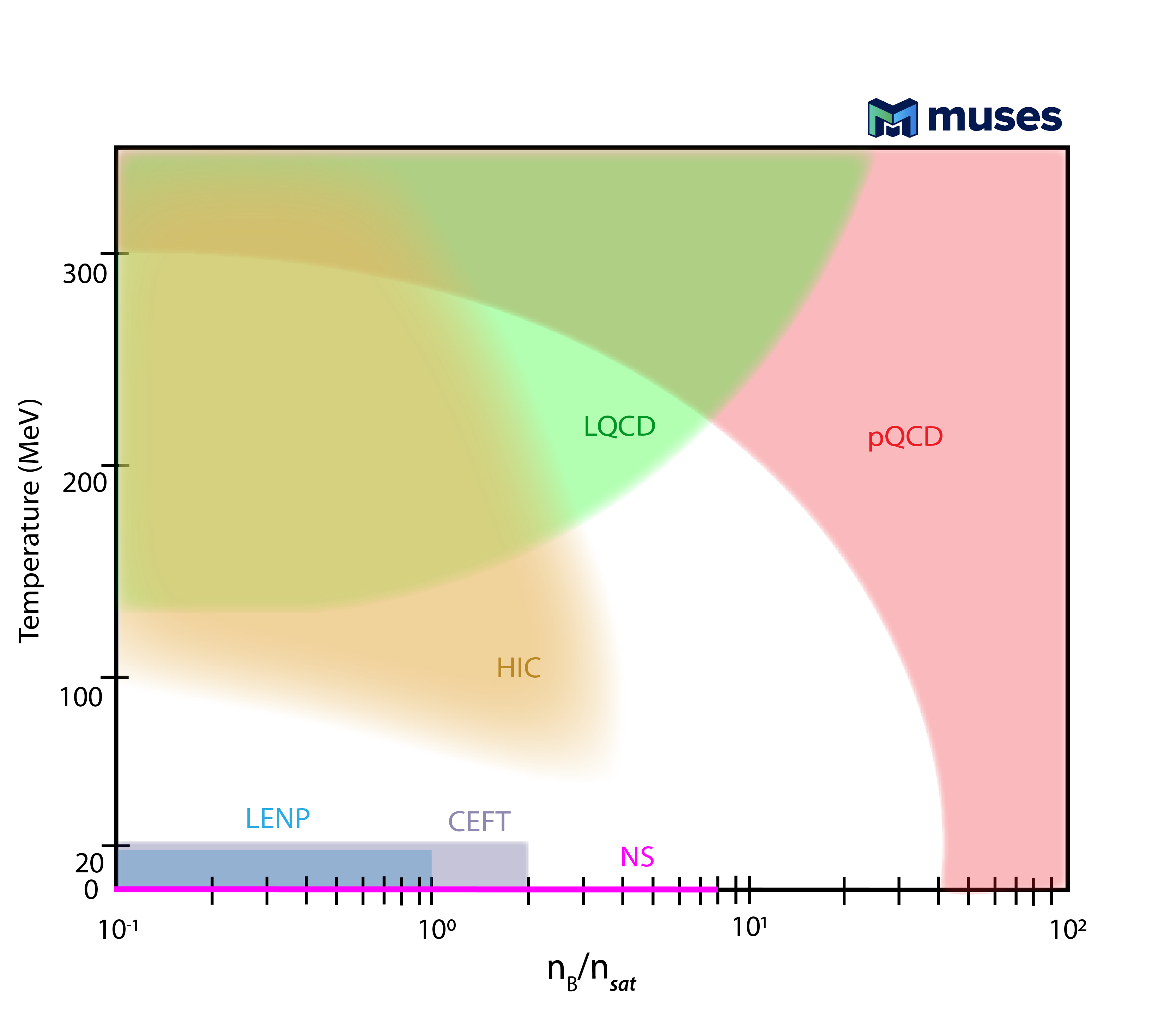
Figure 1: Regions of the QCD phase diagram where constraints from heavy-ion collisions (HIC), lattice QCD (LQCD), perturbative QCD (pQCD), low-energy heavy-ion collisions (LENP), chiral effective field theory ($\chi$EFT), and astrophysics (neutron stars, NS) are available.

II.5 Experimental constraints: heavy-ion collisions

In the laboratory, heavy-ion collisions probe finite temperatures in the range of $T\sim 50-650$ MeV, depending on the center of mass beam energy $\sqrt{s_{NN}}$, such that higher $\sqrt{s_{NN}}$ probe high temperatures and lower $\sqrt{s_{NN}}$ probe lower temperatures. The temperature and density of the system vary in space and time throughout the evolution, which is the hottest at early times. Depending on the choice of the experimental observables, one can obtain information at different temperatures and densities within the collisions. The final distribution of hadrons reflects the temperature and chemical potentials at chemical freeze-out (although certain momentum dependent observables are also sensitive to the kinetic freeze-out, see e.g. Adamczyk et al. (2017) for a comparison between chemical and kinetic freeze-out).

When temperatures are high enough (i.e., high $\sqrt{s_{NN}}$) for a quark-gluon plasma to be produced, such that hydrodynamics is a good dynamical description, lowering $\sqrt{s_{NN}}$ corresponds to a lower initial temperature, a lower freeze-out temperature, and a larger $n_{B}$. However, for very low beam energies, below $\sqrt{s_{NN}}\lesssim 4-7$ GeV, the hadron gas phase dominates, such that hadron transport models may be used. This then means that higher $\sqrt{s_{NN}}$ reaches larger $n_{B}$ whereas lower $\sqrt{s_{NN}}$ reach a smaller range of $n_{B}$. The exact switching point from a quark-gluon plasma dominated- to hadronic-dominated dynamical description is unknown and still hotly debated within the community. The initial collision temperature $T_{0}$ is model-dependent, so we do not include estimates for it in this work. The freeze-out temperature, however, can be more directly extracted from experimental data (with certain caveats that we will explain here) using particle yields and assuming thermal equilibrium at freeze-out. Additionally, the emission of photons and lepton pairs (dileptons), which are immune to strong interactions and can traverse the QGP, can be used to extract average temperatures at different points in the heavy-ion collision evolution, which can be used to pin down the temperature evolution Strickland (1994); Schenke and Strickland (2007); Martinez and Strickland (2008); Dion et al. (2011); Shen et al. (2014); Gale et al. (2015); Bhattacharya et al. (2016); Ryblewski and Strickland (2015); Paquet et al. (2016); Kasmaei and Strickland (2019, 2020). On the other hand, the extraction of $n_{B}$ is more model dependent. If a QCD critical point exists, then susceptibilities of the pressure will diverge exactly at the critical point and may have non-trivial behavior in the surrounding critical region Stephanov (2009); Parotto et al. (2020); Mroczek et al. (2021). In equilibrium, these would determine the cumulants of the distribution of protons, such as the kurtosis. Measurements of the kurtosis Adam et al. (2021a); Abdallah et al. (2023a); Adamczewski-Musch et al. (2020a); Acharya et al. (2020a), 6th-order cumulants Abdallah et al. (2021a), and fluctuations of light nuclei STA (2022) exist from BES-I across a variety of beam energies with large statistical error bars. BES-II Tlusty (2018) will significantly improve the measurement precision. However, the data has not yet been released.

Looking to the future, the Compressed Baryonic Matter (CBM) Experiment at FAIR (GSI, Germany) will be an experimental facility that will be dedicated to explore low beam energies in fixed target mode with high luminosity, i.e., with a high collision rate Spies (2022). CBM Lutz et al. (2009b); Durante et al. (2019) will allow us to constrain the EoS at high $\mu_{B}$ and moderate temperatures. Eventually, from the wealth of experimental data in heavy-ion collisions, it will be possible to extract an EoS using model-to-data comparisons. However, that will require more sophisticated dynamical models that do not yet exist Bluhm et al. (2020). It has already been identified that the azimuthal anisotropies of the momentum distribution of particles in collisions, otherwise known as flow harmonics, are sensitive to the EoS at these low beam energies Danielewicz et al. (2002); Spieles and Bleicher (2020). However, there are still significant questions remaining about the correct dynamical model and other free parameters such as transport coefficients. Depending on the model assumptions, one can obtain radically different posteriors of the EoS, or find different EoSs consistent with the data at these beam energies (a few examples include comparing the different results and conclusions from Danielewicz et al. (2002); Spieles and Bleicher (2020); Schäfer et al. (2022); Shen and Schenke (2022); Oliinychenko et al. (2022)). Thus, in this work, we will only include a discussion on some of the key experimental measurements but cannot yet clarify the precise implications of the data.

II.6 Experimental constraints: low-energy nuclear physics

At significantly lower beam energies (approaching the $T\rightarrow 0$ limit) there are a number of experiments that probe dense matter. These experiments study the properties of nuclei at (or near) saturation density. While most nuclei contain symmetric nuclear matter such that $Y_{Q}\sim 0.5$, heavy nuclei become more neutron-rich and may reach $Y_{Q}\sim 0.4$, while unstable nuclei close to the neutron drip line have much smaller values of $Y_{Q}$. However, neutron stars are composed of primarily asymmetric nuclear matter, with $Y_{Q}\sim 0.001-0.2$. Thus, one can use a Taylor series to expand between symmetric and asymmetric matter, known as the symmetry energy expansion. In this case, a few of its coefficients can be inferred from experimental measurements of, e.g., the neutron skin. Symmetric-matter properties include binding energy per nucleon, compressibility, and saturation density, and can also be inferred, together with the EoS. However, in this case there is model dependence which can be investigated by using different kinds of models.

In addition to the compressibility and the binding energy per nucleon, the effective mass of nucleons at saturation was shown to be important to study the nuclear EoS of hot stars Raduta et al. (2021), the EoS of neutron stars with exotic particles at finite temperature Raduta (2022), thermal effects in supernovae Constantinou et al. (2015), and neutron-star mergers (see Raithel et al. (2019) and references therein). Nevertheless, the experimental determination of this quantity still includes large uncertainties and, therefore, will not be discussed in this review.

Beyond nucleons, properties of hyperons and $\Delta$-baryons can also be determined for symmetric matter. The most useful observable to constrain effective models is optical potentials at $n_{sat}$, which provides the result of the balance between attractive and repulsive strong interactions. At finite temperature, there is also data concerning the critical point for the liquid-gas phase transition Elliott et al. (2012), where nuclei turn into bulk hadronic matter.

II.7 Experimental constraints: astrophysics

The high baryon density inside neutron stars makes them a natural laboratory to understand strong interaction physics under conditions that are impossible to achieve in a laboratory setting. Neutron stars are the end-life of massive stars, which run out of fuel for fusion and collapse gravitationally, violently exploding as supernovae. As a result, the cores of the remnant neutron stars possess densities of the order of several times $n_{sat}$. Neutron stars are stratified according to density, with different types of co-existing phases categorized according to the radial coordinate (see Fig. 2). The outermost layer is the atmosphere, with a thickness of a few centimeters, which contains mostly hydrogen, helium, and carbon atoms. A little bit deeper, in the outer crust, electrons disassociate from specific nuclei and the Fermi energy is large enough for stable nuclei to contain a larger number of neutrons. In the inner crust, neutrons start to “drip out” of nuclei and, as a result, matter becomes a mixture of free electrons, free neutrons, and nuclei. At even higher densities in the outer core, above $\sim n_{sat}$, matter turns into a neutron–rich “soup” with no isolated nuclei. Going deeper into higher densities for the inner core, at about $2~{}n_{sat}$, hyperons, $\Delta$’s, and meson condensates may appear and, eventually, deconfined quark matter may form. Regardless of the phase, fully evolved neutron stars fulfill chemical equilibrium and charge neutrality, either locally or globally, with mixtures of phases occurring in the latter case.

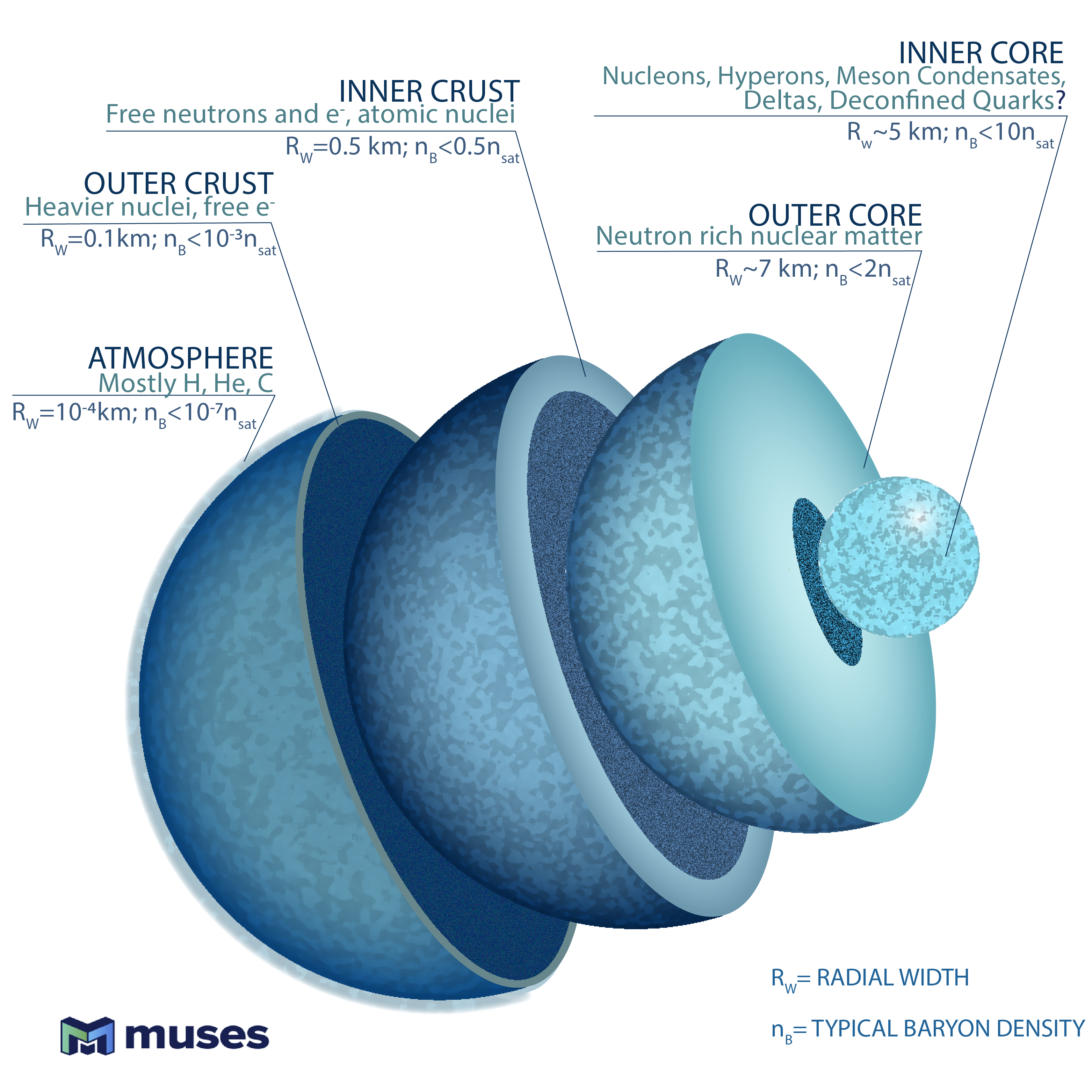
Figure 2: Composition of a typical neutron star.

The EoS is related to microscopic equilibrium properties (pressure, energy density, etc.). Therefore, the nuclear EoS is not directly comparable to astrophysical observations, but it serves as an important input in calibrated models to calculate experimental observables, such as mass-radius relationships of compact stars. This is achieved by solving the Tolman-Oppenheimer-Volkoff (TOV) equations Tolman (1939); Oppenheimer and Volkoff (1939), which are valid as long as rotational frequency ($\nu$) and magnetic field ($B$) effects are not significant. These results can be compared with astrophysical observations from neutron-star electromagnetic emissions, usually radio and X-ray, and most recently, gravitational wave emission from neutron-star mergers. In particular, observations from the National Radio Astronomy Observatory’s Green Bank Telescope (GBT) Demorest et al. (2010), NASA’s Neutron Star Interior Composition Explorer (NICER) Gendreau et al. (2016); Baubock et al. (2015); Miller (2016); Ozel et al. (2016), and NSF’s Laser Interferometer Gravitational-wave Observatory (LIGO) together with VIRGO Abbott et al. (2017a, b); Gendreau et al. (2016) put strong constraints on the EoS Gendreau et al. (2016); Annala et al. (2018). Many EoS models have been updated since these observations were made, to be in agreement with observations Baym et al. (2018).

The most accurate neutron-star mass estimates come from the timing of radio pulsars in orbital systems with relativistic dynamical effects Antoniadis et al. (2013); Cromartie et al. (2019); Fonseca et al. (2021); they inform the EoS insofar as they set a lower bound on the maximum mass it must be able to support against gravitational collapse. The most reliable radius measurements stem from X-ray pulse profile modeling of rotating neutron stars Miller et al. (2019); Riley et al. (2019); Miller et al. (2021); Riley et al. (2021), and constrain the mass-radius relation predicted by the EoS. Meanwhile, gravitational-wave observations of merging neutron stars constrain the EoS via their tidal deformability Abbott et al. (2017a, 2018, 2019, 2020a). If the gravitational waves are accompanied by a kilonova counterpart, as was the case for the binary neutron-star merger GW170817 Abbott et al. (2017b), the lightcurve and spectrum of the electromagnetic emission, as well as its implications for the fate of the merger remnant, also inform the EoS Bauswein et al. (2017); Margalit and Metzger (2017); Radice et al. (2018); Rezzolla et al. (2018); Ruiz et al. (2018); Shibata et al. (2017). Eventually, upgraded gravitational wave detectors will also be able to detect the post-merger signal Carson et al. (2019) (the post-merger starts at the point where the two neutron stars touch). This signal is also sensitive to finite temperature effects that may even reach temperatures and densities similar to heavy-ion collisions Adamczewski-Musch et al. (2019a), as well as potential out-of-equilibrium effects due to the long-time scales associated with weak interactions Alford et al. (2018, 2019); Alford and Harris (2019); Alford et al. (2021); Gavassino et al. (2021); Celora et al. (2022); Most et al. (2022).

II.8 Organization of the paper

This review paper aims at compiling up-to-date constraints from high-energy physics, nuclear physics, and astrophysics that relate to the EoS and are, therefore, fundamental to the understanding of current and future data from heavy-ion collisions to gravitational waves, making them relevant to a very broad community. Additionally, precise knowledge of the dense and hot matter EoS can help physicists to look beyond the standard model either for dark matter, which may accumulate in or around neutron stars, or for modified theories of gravity.

The paper is organized as follows: we first discuss the theoretical constraints of lattice III and perturbative QCD IV, followed by $\chi$EFT V. Then, we discuss experimental constraints from heavy-ion collisions VI, (isospin symmetric and asymmetric) low-energy nuclear physics VII, and astrophysical observations VIII. We provide a future outlook in section IX, since a significant amount of new data is anticipated over the next decade.

III Theoretical Constraints: Lattice QCD

Lattice QCD is the most suitable method to study strong interactions around and above the deconfinement phase transition region in the QCD phase diagram, due to its non-perturbative nature Drischler et al. (2021b). As discussed in the introduction, due to the sign problem, first-principles lattice QCD results for the EoS at finite $\mu_{B}$ are currently restricted. Since direct lattice simulations at $\mu_{B}=0$ and imaginary $\mu_{B}$ are feasible, observables can be extrapolated using techniques involving zero or imaginary chemical potential simulations, i.e., analytical continuation, Taylor series and other alternative expansions. In this section, we present various constraints on the EoS, BSQ (baryon number, strangeness, and electric charge) susceptibilities, and partial pressures evaluated using lattice QCD.

III.1 Equation of state

In Refs. Borsanyi et al. (2014a); Bazavov et al. (2014), the EoS was obtained in lattice QCD simulations at $\mu_{B}=0$. It was found that the rigorous continuum extrapolation results for 2+1 quark flavors are perfectly compatible with previous continuum estimates based on coarser lattices Aoki et al. (2006); Borsanyi et al. (2010). The obtained pressure, entropy density, and interaction measure are displayed in the left panel of Fig. 3 alongside the predictions of the hadron resonance gas (HRG) model at low temperatures and the Stefan-Boltzmann (or conformal) limit of a non-interacting massless quarks gas at high $T$. They show full agreement with HRG results in the hadronic phase, and reach about 75% of the Stefan-Boltzmann limit at $T\simeq 400$ MeV.

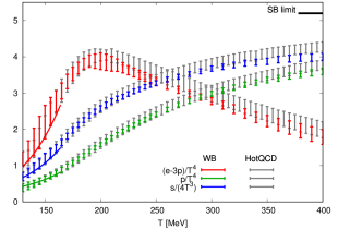
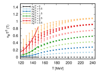
Figure 3: Left: from Ref. Ratti (2018). Comparison between the lattice QCD EoS at $\mu_{B}=0$ from the WB collaboration Borsanyi et al. (2014a) (colored points) and the HotQCD one Bazavov et al. (2014) (gray points). Right: from Ref. Borsányi et al. (2021). Baryonic density as a function of the temperature, for different values of $\mu_{B}/T$. At low temperature, full lines show results from the HRG model.

Furthermore, a Taylor series can be utilized to expand many observables to finite $\mu_{B}/T$

$$\frac{p(T,\mu_{B},\mu_{Q},\mu_{S})}{T^{4}}=\sum_{i,j,k}\frac{1}{i!j!k!}\chi_{ijk}^{BQS}\left(\frac{\mu_{B}}{T}\right)^{i}\left(\frac{\mu_{Q}}{T}\right)^{j}\left(\frac{\mu_{S}}{T}\right)^{k}\ ,$$ (2)

where the susceptibilities $\chi_{ijk}^{BQS}$ are defined as follows

$$\chi_{lmn}^{BSQ}=\frac{\partial^{l+m+n}(p/T^{4})}{\partial(\mu_{B}/T)^{l}\partial(\mu_{S}/T)^{m}\partial(\mu_{Q}/T)^{n}}\ .$$ (3)

They were obtained from lattice QCD calculations up to $\mathcal{O}(\mu_{B}/T)^{4}$ for the full series of coefficients and up to $\mathcal{O}(\mu_{B}/T)^{8}$ for some of the coefficients. The range of applicability of the Taylor expansion has recently been extended from $\mu_{B}/T\leq 2$ Guenther et al. (2017); Bazavov et al. (2017) to $\mu_{B}/T\leq 2.5$ Bollweg et al. (2022). Isentropic trajectories in the $T-\mu_{B}$ plane have been extracted in Ref. Guenther et al. (2017), for which the starting points are the freeze-out parameters at different collision energies at RHIC Alba et al. (2014). Strangeness neutrality and electric charge conservation were enforced by tuning the strange and electric charge chemical potentials, $\mu_{S}(\mu_{B},T)$ and $\mu_{Q}(\mu_{B},T)$, to reproduce the conditions $Y_{S}=0$ and $Y_{Q}=0.4$ Guenther et al. (2017).

A new expansion scheme for extending the EoS of QCD to unprecedentedly large baryonic chemical potential up to $\mu_{B}/T<3.5$ has been proposed recently Borsányi et al. (2021). The drawbacks of the conventional Taylor expansion approach, such as the challenges involved in carrying out such an expansion with a constrained number of coefficients and the low signal-to-noise ratio for the coefficients themselves, are significantly reduced in this new scheme Borsányi et al. (2021). In the hadronic phase, a good agreement is found for the thermodynamic variables with HRG model results. This scheme is based on the following identity

$$\frac{\chi_{1}^{B}(T,\mu_{B})}{\mu_{B}/T}=\chi_{2}^{B}(T^{\prime},0)\ ,$$ (4)

with

$$T^{\prime}(T,\mu_{B})=T(1+\kappa_{2}^{BB}(T)\left(\frac{\mu_{B}}{T}\right)^{2}+\kappa_{4}^{BB}(T)\left(\frac{\mu_{B}}{T}\right)^{4}+\mathcal{O}((\mu_{B}/T)^{6})\ .$$ (5)

The baryonic density as a function of the temperature for different values of $\mu_{B}/T$ from Ref. Borsányi et al. (2021) is shown in the right panel of Fig. 3. This extrapolation method was then generalized to include the strangeness neutrality condition Borsanyi et al. (2022), which requires $\mu_{S}\neq 0$. The extrapolation approach is devoid of the unphysical oscillations that afflict fixed order Taylor expansions at higher $\mu_{B}$, even in the strangeness neutral situation. Effects beyond strangeness neutrality are estimated by computing the baryon-strangeness correlator to strangeness susceptibility ratio $\frac{\chi^{BS}_{11}}{\chi^{S}_{2}}$ (discussed in the following subsection) at finite real $\mu_{B}$ on the strangeness neutral line. This permits a leading order extrapolation in the ratio $R={\chi^{S}_{1}}/{\chi^{B}_{1}}$ Borsanyi et al. (2022).

III.2 BSQ susceptibilities

Fluctuations of different conserved charges have been postulated as a signal of the deconfinement transition because they are sensitive probes of quantum numbers and related degrees of freedom. In heavy-ion collisions, one needs to relate fluctuations of net baryon number, strangeness, and electric charge with the event-by-event fluctuations of particle species. Nondiagonal correlators of conserved charges, like fluctuations, are useful for studying the chemical freeze-out in heavy-ion collisions. In thermal equilibrium, they may be estimated using lattice simulations and linked to moments of event-by-event multiplicity distributions. They are defined as derivatives of the pressure with respect to the chemical potentials according to Eq. (3). The quark number chemical potentials appear as parameters in the Grand Canonical partition function. The derivative of this function with respect to these chemical potentials yields the susceptibilities and the nondiagonal correlators of the quark flavors. Quark flavor chemical potentials can be related to the conserved charge ones through the following relationships: $\mu_{u}=\frac{1}{3}\mu_{B}+\frac{2}{3}\mu_{Q}$, $\ \mu_{d}=\frac{1}{3}\mu_{B}-\frac{1}{3}\mu_{Q}$, and $\ \mu_{s}=\frac{1}{3}\mu_{B}-\frac{1}{3}\mu_{Q}-\mu_{S}$.

For $T=125–400$ MeV and at $\mu_{B}=\mu_{S}=\mu_{Q}=0$, the Wuppertal-Budapest lattice QCD collaboration computed the non-diagonal (us) and diagonal (B,s,Q,I,u) susceptibilities for a system of 2+1 staggered quark flavors Borsanyi et al. (2012), where I stands for isospin. Selected susceptibilities are shown in the left panel of Fig. 4. A Symanzik-improved gauge and a stout-link improved staggered fermion action were used in this analysis. The ratios of fluctuations were found, whose behavior may be recreated using hadronic observables, i.e. proxies, to compare either to lattice QCD findings or experimental observations Bellwied et al. (2020).

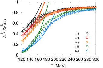
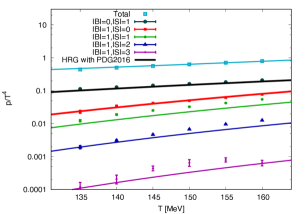
Figure 4: Left: from Ref. Borsanyi et al. (2012). Baryon number, strange quark, electric charge, isospin number, and up quark susceptibilities as functions of the temperature at $\mu_{B}=0$. Right: from Ref. Alba et al. (2017). Compilation of partial pressures for different hadron families as functions of the temperature.

Continuum extrapolated lattice QCD findings for $\chi_{2,2}^{u,s},~{}\chi_{2,2}^{u,d},~{}\chi_{1,1}^{u,d},~{}\chi_{4}^{u},~{}\chi_{4}^{B}$ were presented in Ref. Bellwied et al. (2015). Second and fourth-order cumulants of conserved charges were constructed in a temperature range spanning from the QCD transition area to the region of resummed perturbation theory. It was found that, in the hadronic phase ($T\sim 130$ MeV), the HRG model predictions accurately reflect the lattice data, whereas in the deconfined region ($T\gtrsim 250$ MeV), a good agreement was found with three loop hard-thermal-loop (HTL) outcomes Bellwied et al. (2015). Different diagonal and non-diagonal fluctuations of conserved charges are estimated up to sixth-order on a lattice size of 48${}^{3}\times$ 12 Borsanyi et al. (2018). Higher-order fluctuations at zero baryon/charge/strangeness chemical potential are calculated. The ratios of baryon-number cumulants as functions of $T$ and $\mu_{B}$ are derived from these correlations and fluctuations, which fulfill the experimental criteria of proton/baryon ratio and strangeness neutrality and in turn, describe the observed cumulants as functions of collision energy from the STAR collaboration Borsanyi et al. (2018). Ratios of fourth-to-second order susceptibilities for light and strange quarks were presented in Ref. Bellwied et al. (2013).

III.3 Partial pressures

Under the assumption that the hadronic phase can be treated as an ideal gas of resonances, and using lattice simulations, the partial pressures of hadrons were determined with various strangeness and baryon number contents. To explain the difference between the results of the HRG model and lattice QCD for some of them, the existence of missing strange resonances was proposed Bazavov et al. (2013a); Alba et al. (2017). Note that partial pressures are only possible within the hadron resonance gas phase because i.) they require hadronic degrees-of-freedom and ii.) they are applicable under the assumption that the pressure can be written as separable components by the quantum number of the hadrons, i.e.,

$$P(\hat{\mu}_{B},\hat{\mu}_{S}) = P^{BS}_{00}+P^{BS}_{10}\cosh(\hat{\mu}_{B})+P^{BS}_{01}\cosh(\hat{\mu}_{S})+P^{BS}_{11}\cosh(\hat{\mu}_{B}-\hat{\mu}_{S})$$ (6)

$$+ P^{BS}_{12}\cosh(\hat{\mu}_{B}-2\hat{\mu}_{S})+P^{BS}_{13}\cosh(\hat{\mu}_{B}-3\hat{\mu}_{S})\ ,$$

where the coefficients $P^{BS}_{ij}$ indicate the baryon number $i$ and strangeness $j$ of the family of hadrons for which the partial pressure is being isolated, and the dimensionless chemical potentials are written as $\hat{\mu}=\mu/T$. The calculations were made feasible by taking imaginary values of strange chemical potential in the simulations. For strange mesons, more interaction channels should be incorporated into the HRG model, in order to explain the lattice data Alba et al. (2017). The right panel of Fig. 4 shows a compilation of these partial pressures.

III.4 Pseudo phase-transition line

In a crossover there is no sudden jump in the first derivatives of the pressure. Nevertheless, a pseudo-phase transition line can be calculated based on where the order parameters change more rapidly. The exact location of the QCD transition line is a hot topic of research in the field of strong interactions. The most recent results are contained in Ref. Borsanyi et al. (2020). The transition temperature as a function of the chemical potential can be parametrized as

$$\frac{T_{c}(\mu_{B})}{T_{c}(\mu_{B}=0)}=1-\kappa_{2}\left(\frac{\mu_{B}}{T_{c}(\mu_{B})}\right)^{2}-\kappa_{4}\left(\frac{\mu_{B}}{T_{c}(\mu_{B})}\right)^{4}+\dots\ .$$ (7)

The crossover or pseudo-critical temperature $T_{c}$ has been determined with extreme accuracy and extrapolated from imaginary up to real $\mu_{B}\approx 300$ MeV. Additionally, the width of the chiral transition and the peak value of the chiral susceptibility were calculated along the crossover line. Both of them are constant functions of $\mu_{B}$. This means that, up to $\mu_{B}=300$ MeV, no sign of criticality has been observed in lattice results. In fact, at the critical point the height of the peak of the chiral susceptibility would diverge and its width would shrink. The small error reflects the most precise determination of the $T-\mu_{B}$ phase transition line using lattice techniques. Besides $T_{c}=158\pm 0.6$ MeV, the study provides updated results for the coefficients $\kappa_{2}=0.0153\pm 0.0018$ and $\kappa_{4}=0.00032\pm 0.00067$ Borsanyi et al. (2020). Similar coefficients for the extrapolation of the transition temperature to finite strangeness, electric charge, and isospin chemical potentials were obtained in Ref. Bazavov et al. (2019a), and are displayed in Table 2.

$\kappa_{2}^{B}$	$\kappa_{4}^{B}$	$\kappa_{2}^{S}$	$\kappa_{4}^{S}$	$\kappa_{2}^{Q}$	$\kappa_{4}^{Q}$	$\kappa_{2}^{I}$	$\kappa_{4}^{I}$
0.016(6)	0.001(7)	0.017(5)	0.004(6)	0.029(6)	0.008(1)	0.026(4)	0.005(7)

Table 2: Continuum-extrapolated values of $\kappa_{2}^{X}$ and $\kappa_{4}^{X}$ (with $\mu_{Q}=\mu_{S}=0$ for $X=B$,
$\mu_{B}=\mu_{Q}=0$ for $X=S$ and $\mu_{B}=\mu_{S}=0$ for $X=Q,I$) from Bazavov et al. (2019a).

III.5 Limits on the critical point location

As mentioned in the previous subsection, in Ref. Borsanyi et al. (2020), by extrapolating the proxy for the transition width as well as the height of the chiral susceptibility peak from imaginary to real $\mu_{B}$, the strength of the phase transition was evaluated and no indication of criticality was found up to $\mu_{B}\approx$ 300 MeV. On the other hand, a phase transition temperature at $\mu_{B}=0$ of $T_{c}=132^{+3}_{-6}$ MeV was found in the chiral limit by the HotQCD collaboration using lattice QCD calculations with “rooted” staggered fermions Ding et al. (2019). This transition temperature is computed with two massless light quarks and a physical strange quark based on two unique estimators. Since the curvature of the phase diagram is negative, a critical point in the chiral limit would sit at a temperature smaller than this one. The expectation is that the temperature of the critical point at physical quark masses has to be smaller than the one of the critical point in the chiral limit, and therefore definitely smaller than $T_{c}=132^{+3}_{-6}$ MeV.

IV Theoretical Constraints: Perturbative QCD

It is possible to compute analytically the QCD EoS directly from the QCD Lagrangian using finite temperature/density perturbation theory. However, in thermal and chemical equilibrium, when $T\gg\mu_{i}$ (with quark chemical potentials $\mu_{i}$), one finds that the naive loop expansion of physical quantities is ill-defined and diverges beyond a given loop order, which depends on the quantity under consideration. In the calculation of QCD thermodynamics, this stems from uncanceled infrared (IR) divergences that enter the expansion of the partition function at three-loop order. These IR divergences are due to long-distance interactions mediated by static gluon fields and result in contributions that are non-analytic in the strong coupling constant $\alpha_{s}=g^{2}/4\pi$, e.g., $\alpha_{s}^{3/2}$ and $\log(\alpha_{s})$, unlike vacuum perturbation expansions which involve only powers of $\alpha_{s}$.

It is possible to understand at which perturbative order terms that are non-analytic in $\alpha_{s}$ appear by considering the contribution of non-interacting static gluons to a given quantity. For simplicity, we now discuss the case of $\mu_{B}=0$ for this argument, but the same holds true at finite chemical potential. For the pressure of a gas of gluons one has $P_{\text{gluons}}\sim\int d^{3}p\,p\,f_{B}(E_{p})$, where $f_{B}$ denotes a Bose-Einstein distribution function and $E_{p}$ is the energy of the in-medium gluons. The contributions from the momentum scales $\pi T$, $gT$ and $g^{2}T$ can be expressed as

$$P_{\text{gluons}}^{p\sim\pi T} \sim T^{4}f_{B}(\pi T)\;\sim\;T^{4}+{\mathcal{O}}(g^{2})\,,$$ (8)

$$P_{\text{gluons}}^{p\sim gT} \sim (gT)^{4}f_{B}(gT)\;\sim\;g^{3}T^{4}+{\mathcal{O}}(g^{4})\,,$$ (9)

$$P_{\text{gluons}}^{p\sim g^{2}T} \sim (g^{2}T)^{4}f_{B}(g^{2}T)\;\sim\;g^{6}T^{4}\ ,$$ (10)

where we have used the fact that $f_{B}(E)\sim T/E$ if $E\ll T$. This fact is of fundamental importance, since it implies that when the energy/momentum are soft, corresponding to electrostatic contributions $p_{\text{soft}}\sim gT$, one receives an enhancement of $1/g$ compared to contributions from hard momenta, $p_{\text{hard}}\sim T$, due to the bosonic nature of the gluon. For ultrasoft (magnetostatic) momenta, $p_{\text{ultrasoft}}\sim g^{2}T$, the contributions are enhanced by $1/g^{2}$ compared to the naive perturbative order. As Eqs. (8)-(10) demonstrate, it is possible to generate contributions of the order $g^{3}\sim\alpha_{s}^{3/2}$ from soft momenta and, in the case of the pressure, although perturbatively enhanced, ultrasoft momenta only start to play a role at order $g^{6}\sim\alpha_{s}^{3}$.

Due to the infrared enhancement of electrostatic contributions, there is a class of diagrams called hard-thermal-loop (HTL) graphs that have soft external momenta and hard internal momenta that need to be resummed to all orders in the strong coupling Braaten and Pisarski (1990a, b, c). There are now several schemes for carrying out such soft resummations Arnold and Zhai (1994, 1995); Zhai and Kastening (1995); Braaten and Nieto (1995, 1996a); Kajantie et al. (1997); Andersen et al. (1999, 2000a, 2000b); Blaizot et al. (1999a, b, 2001a, 2001b); Andersen et al. (2002, 2004, 2010b, 2011c); Haque et al. (2014a, b). We note however, that even with such resummations, if one casts the result as a strict power series in the strong coupling constant the convergence of the perturbative series for the QCD free energy is quite poor. To address this issue, one must treat the soft sector non-perturbatively and re-sum contributions to all orders in the strong coupling constant. This can be done using effective field theory methods Ghiglieri et al. (2020), approximately self-consistent two-particle irreducible methods Blaizot et al. (1999a, b, 2001a, 2001b), or the hard-thermal-loop perturbation theory reorganization of thermal field theory Andersen et al. (1999, 2000a, 2002, 2004, 2010b, 2011c); Haque et al. (2014a, b).

Thus, the calculation of the QCD EoS requires all-orders resummation, which can be accomplished in a variety of manners. Despite the fact that different methods exist, they all rely fundamentally on the use of so-called hard-thermal- or hard-dense-loops, which self-consistently include the main physical effect of the generation of in-medium gluon and quark masses at the one-loop level. By reorganizing the perturbative calculation of the QCD EoS around the high-temperature hard-loop limit of quantum field theory, the convergence of the perturbative series can be extended to phenomenologically relevant temperatures and densities. Below we summarize the results that have been obtained and compared to lattice QCD calculations where available.

IV.1 The resummed perturbative QCD EoS

The QCD EoS of deconfined quark matter at high chemical potential can be evaluated in terms of perturbative series in the running coupling constant $\alpha_{s}$. As a result, the neutron-star EoS can be studied using the weak coupling expansion Kurkela et al. (2014); Annala et al. (2018); Shuryak (1978); Zhai and Kastening (1995); Braaten and Nieto (1996a, b); Arnold and Zhai (1995, 1994); Toimela (1985); Kapusta (1979); Annala et al. (2020); Kurkela et al. (2014, 2010); Freedman and McLerran (1977b, c). The EoS and trace anomaly of deconfined quark matter have been calculated to three-loop order using HTL perturbation theory framework at small $\mu_{B}$ and arbitrary $T$. Renormalization of the vacuum energy, the HTL mass parameters, and $\alpha_{s}$ eliminate all UV divergences. The three-loop results for the thermodynamic functions are observed to be in agreement with lattice QCD data for $T$ $\gtrsim$ 2-3 $T_{c}$ after choosing a suitable mass parameter prescription Andersen et al. (2011c). Furthermore, the QCD thermodynamic potential at nonzero temperature and chemical potential(s) has been calculated using N$2$LO at three-loop HTL perturbation theory which was used further to calculate the pressure, entropy density, trace anomaly, energy density, and speed of sound, $c_{s}$, of the QGP Haque et al. (2014b). These findings were found to be in very good agreement with the data obtained from lattice QCD using the central values of the renormalization scales. This is illustrated in Figs. 5 and 6, which present comparisons of the resummed perturbative results with lattice data for the pressure and fourth-order baryonic and light-quark susceptibilities. In these Figures, HTLpt corresponds to the N2LO hard thermal loop perturbation theory calculation of the EoS and EQCD corresponds to a resummed N2LO electric QCD effective field theory calculation of the same. The shaded bands indicate the size of the uncertainty due to the choice of renormalization scale.

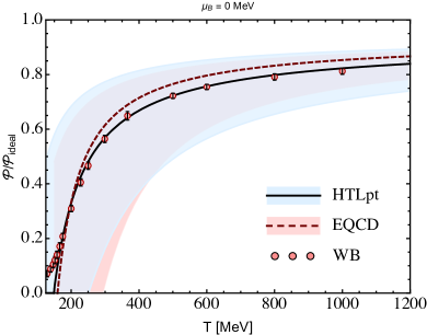
Figure 5: Left: The resummed QCD pressure for $\mu_{B}=0$ obtained using the three-loop EQCD and HTL perturbation theory results with lattice data from the Wuppertal-Budapest (WB) collaboration Borsanyi et al. (2010). Right: The second-order light quark (and baryon) number susceptibilities. Lattice data are from the WB Borsanyi (2013); Borsanyi et al. (2013) and BNLB collaborations Bazavov et al. (2013b).

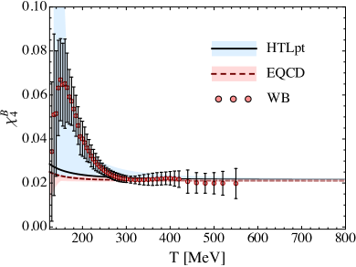
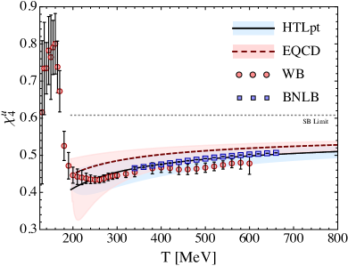
Figure 6: Left: The 4th baryon number susceptibility. Right: The 4th light quark number susceptibility. Lattice data sources are the same as in Fig. 5.

IV.2 The curvature of the QCD phase transition line

In another study, for the second- and fourth-order curvatures of the QCD phase transition line, the N$2$LO HTL perturbation theory predictions were shown. In all three situations, (i) $\mu_{s}=$ $\mu_{l}=\mu_{B}/3$, (ii) $\mu_{s}=0,\mu_{l}=\mu_{B}/3$, and (iii) $S=0,Q/B=0.4,\mu_{l}=\mu_{B}/3$, it was shown that N$2$LO HTL perturbation theory is compatible with the already available lattice computations of $\kappa_{2}$ and $\kappa_{4}$ as defined in Eq. (7) Haque and Strickland (2021). This is illustrated in Fig. 7, which presents comparisons of the resummed perturbative results with lattice data for the coefficients $\kappa_{2}$ and $\kappa_{4}$.

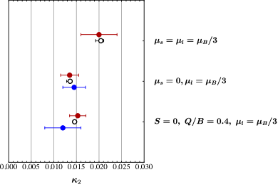
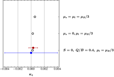
Figure 7: Left: Filled circles are lattice calculations of the quadratic curvature coefficient $\kappa_{2}$ Cea et al. (2016); Bonati et al. (2015, 2018); Borsanyi et al. (2020); Bazavov et al. (2019b), from top to bottom, respectively. Red-filled circles are results obtained using the imaginary chemical potential method and blue-filled circles are results obtained using Taylor expansions around $\mu_{B}=0$. Black open circles are the N$2$LO HTL perturbation theory predictions. Right: Filled circles are lattice calculations of quartic coefficient $\kappa_{4}$ from Refs. Borsanyi et al. (2020); Bazavov et al. (2019b), from top to bottom, respectively. The error bars associated with the HTL perturbation theory predictions result from variations of the assumed renormalization scale.

IV.3 Application at high density

In Ref. Gorda et al. (2021a), at $T=0$, the authors calculated the N$3$LO contribution emerging from non-Abelian interactions among long-wavelength, dynamically screened gluonic fields using the weak-coupling expansion of the dense QCD EoS. In particular, they used the HTL effective theory to execute a comprehensive two-loop computation that is valid for long-wavelength, or soft, modes. In the plot of the EoS, unlike at high temperatures, the soft sector behaves well within cold quark matter, and the novel contribution reduces the renormalization-scale dependence of the EoS at high density Gorda et al. (2021a). Working at exactly zero temperature is often a good approximation for fully evolved neutron stars but for the early stages of neutron-star evolution and neutron-star mergers, it is essential to incorporate temperature effects Shen et al. (1998). However, the inclusion of finite temperature in high-$\mu_{B}$ quark matter gives rise to a technical difficulty for weak coupling expansions. It is no longer sufficient under this regime to handle simply the static sector of the theory nonperturbatively, but the $T=0$ limit’s accompanying technical simplifications are also unavailable. In the EoS plots (see Fig. 8), the breakdown of the weak coupling expansion is observed by a rapid increase in the uncertainty of the result with an increase in temperature for tiny values of $\mu_{B}$ Kurkela and Vuorinen (2016).

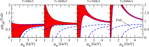
Figure 8: From Ref. Kurkela and Vuorinen (2016). EoS of deconfined quark matter as a function of $\mu_{B}$ at four different temperatures. The new result is shown by the red bands, with the widths resulting from a change in the renormalization scale $\tilde{\Lambda}$ Kurkela and Vuorinen (2016). The corresponding $\mathcal{O}(g^{4})$ result at absolute zero is shown by the dashed blue lines Freedman and McLerran (1977c); Baluni (1978); Vuorinen (2003).

The most up-to-date pQCD results at $T=0$ and finite densities can be found in Gorda et al. (2021b). The EoS derived in these calculations was applicable starting at $n_{B}\sim 40~{}n_{sat}$ and above. However, there is an overall renormalization scale parameter, $X$, that is unknown. One can extrapolate down to lower densities assuming that the speed of sound squared should be bounded by causality and stability, i.e., $0\leq c_{s}^{2}\leq 1$. The results were shown in Komoltsev and Kurkela (2022) where they varied $X$ in the range $1\leq X\leq 4$. The results of the constrained regime can be seen in Fig. 9. Various groups have then used these constraints in their neutron star EoS analyses Marczenko et al. (2023); Somasundaram et al. (2022).

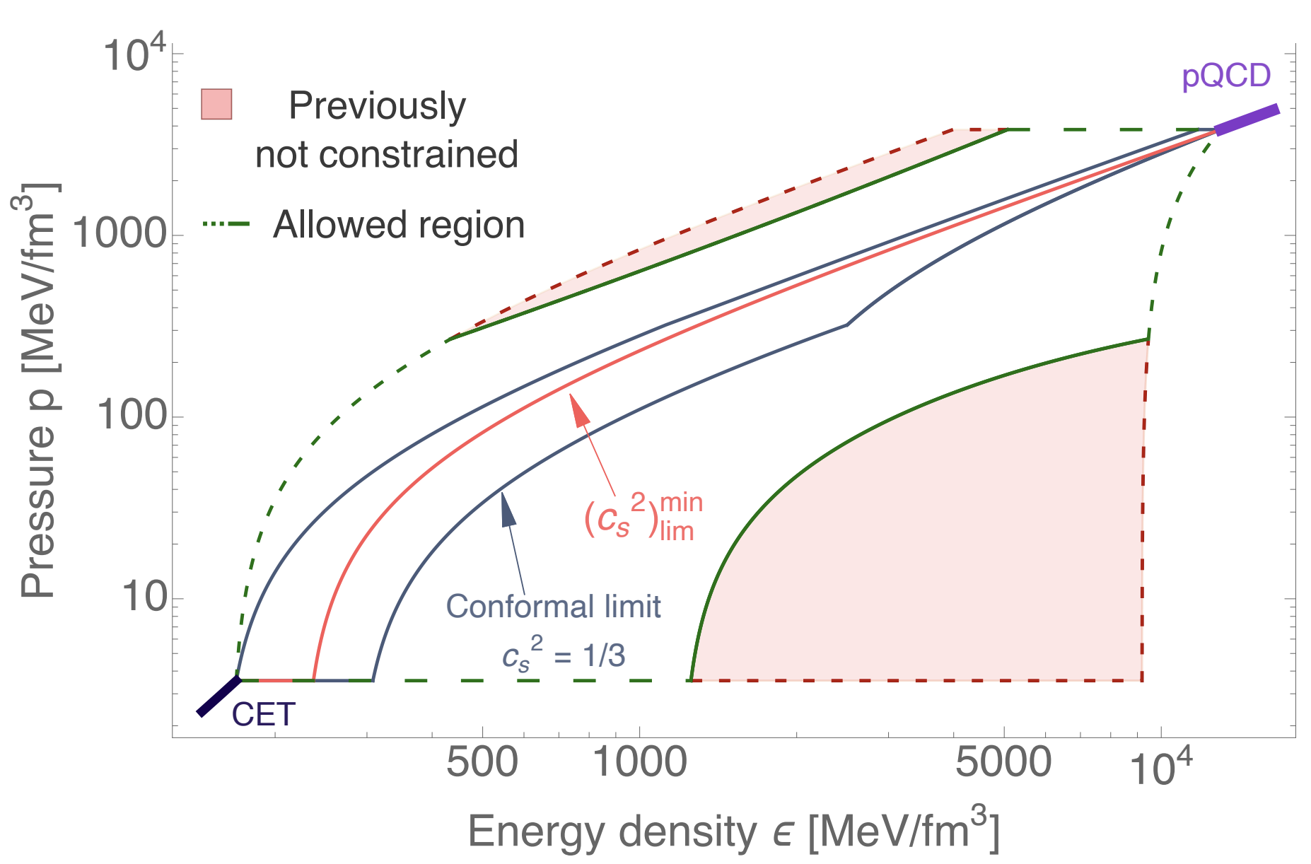
Figure 9: The extracted EoS constraints from pQCD at high $n_{B}$ and $\chi$EFT (see Sec. V for details) are shown. The excluded regions are in pink. Figure taken from Komoltsev and Kurkela (2022).

IV.4 Transport coefficients at finite $T$ and $\mu_{B}$

The quark-gluon plasma probed in heavy-ion collisions is not in equilibrium and viscous effects from shear and bulk viscosities are important for the evolution of the system. At the moment it is not yet possible to reliably compute the shear and bulk viscosities using first principle calculations Meyer (2011). However, it is possible to perform calculations of these coefficients in the weak-coupling limit of QCD. The shear viscosity $\eta$ and relaxation time $\tau_{\pi}$ (the timescale within which the system relaxes towards its Navier-Stokes regime Denicol and Rischke (2021)) are usually related through

$$\tau_{\pi}=C\frac{\eta}{\varepsilon+p}\ ,$$ (11)

where $C$ is a constant determined by the theory. Calculations of $\eta/s$ in QCD have been completed up to NLO (next-to leading order) Ghiglieri et al. (2018a) and the constant $C$ of the relaxation time at NLO Ghiglieri et al. (2018b) for $\mu_{B}=0$, as shown in Fig. 10.

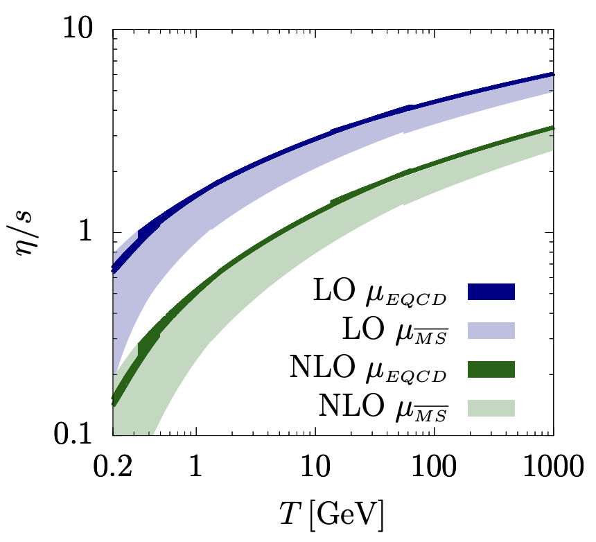
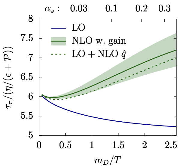
Figure 10: Left: Shear viscosity to entropy density ratio vs. temperature derived from pQCD at LO (leading order) and NLO (next-to leading order) for two different choices of the running coupling for 3 flavors. Figure taken from Ghiglieri et al. (2018a). Right: Coefficient of the relaxation time for shear viscosity at leading order and next-to-leading order as a function of the Debye mass over temperature for QCD with 3 light flavors. Figure taken from Ghiglieri et al. (2018b).

Recently, the first calculations of shear viscosity at leading-log at finite $\mu_{B}$ were performed in QCD in Danhoni and Moore (2023), as shown in Fig. 11.

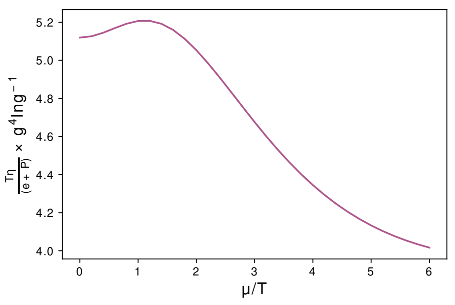
Figure 11: Shear viscosity times temperature divided by the enthalpy versus chemical potential over temperature in 3 flavor QCD. Figure taken from Danhoni and Moore (2023).

Note, however, that at finite $\mu_{B}$ the most natural dimensionless quantity involves the enthalpy ($w=\varepsilon+p$), such that $\eta T/w$ is the relevant quantity (the factor of $T$ is to ensure that it remains dimensionless) to be used Liao and Koch (2010). In the limit of vanishing baryon chemical potential, then

$$\lim_{\mu_{B}\rightarrow 0}\frac{\eta T}{\varepsilon+p}=\frac{\eta}{s}\ ,$$ (12)

such that these results should be smoothly connected regardless of $\mu_{B}$. The relaxation time has not yet been calculated in QCD at finite $\mu_{B}$. Finally we note that, in typical relativistic viscous hydrodynamics simulations performed in heavy-ion collisions, a number of other transport coefficients are also needed. For example, using perturbative QCD, the bulk viscosity has been computed in Arnold et al. (2006), conductivity and diffusion in Arnold et al. (2000), and some second-order transport coefficients can be found in York and Moore (2009). In practice, these perturbatively-determined expressions are not the ones used in simulations, which often rely on simple formulas involving the transport coefficients determined from, for instance, kinetic theory models Denicol et al. (2012, 2014) or holography Kovtun et al. (2005); Finazzo et al. (2015); Rougemont et al. (2017); Grefa et al. (2022), see Everett et al. (2021).

V Theoretical Constraints: Chiral Effective Field Theory

In the opposite regime of low density and temperature, Chiral Effective Field Theory ($\chi$EFT) is used to calculate the EoS relevant around $n_{B}\sim n_{sat}$ of neutron stars. For ab initio $\chi$EFT calculations, it is possible to study the EoS at arbitrary isospin asymmetry at both zero and nonzero temperature Drischler et al. (2014); Wellenhofer et al. (2016); Wen and Holt (2021); Somasundaram et al. (2021). However, in practice it is convenient to first compute the EoS for symmetric nuclear matter ($Y_{Q}=0.5$) and pure neutron matter ($Y_{Q}=0$) and then interpolate between the two using the quadratic approximation for the isospin-asymmetry dependence of the EoS. From the density-dependent symmetry energy, one can extract the coefficients $E_{sym}$, $L$, $K_{sym}$ from $\chi$EFT calculations

$$E_{NS}=E_{Y_{Q}=0.5}+N_{B}\left[E_{sym,sat}+\frac{L_{sat}}{3}\left(\frac{n_{B}}{n_{sat}}-1\right)+\frac{K_{sym,sat}}{18}\left(\frac{n_{B}}{n_{sat}}-1\right)^{2}\right]\big{(}1-2Y_{Q}\big{)}^{2}\ ,$$ (13)

where $E_{NS}$ is the ground-state energy at a given density and isospin asymmetry, $E_{Y_{Q}=0.5}$ is the total energy for isospin-symmetric nuclear matter, $E_{sym,sat}=\left(\frac{E_{Y_{Q}=0}-E_{Y_{Q}=0.5}}{N_{B}}\right)_{n_{sat}}$ is the symmetry energy at saturation, $L_{sat}=3n_{sat}\left(\frac{dE_{sym}}{dn_{B}}\right)_{n_{sat}}$ is the slope of the symmetry energy at saturation, and $K_{sym,sat}=9n_{sat}^{2}\left(\frac{d^{2}E_{sym}}{dn_{B}^{2}}\right)_{n_{sat}}$ is the symmetry energy curvature at saturation. Using this expansion scheme, it is possible to obtain the neutron star outer core EoS with quantified uncertainties from $\chi$EFT. The properties of the low-density crust Lim and Holt (2017); Grams et al. (2022) and the high-density inner core Hebeler et al. (2010); Tews et al. (2018); Lim et al. (2021); Drischler et al. (2021c); Brandes et al. (2023) require additional modeling assumptions.

The energy per baryon of symmetric nuclear matter, $E_{Y_{Q}=0.5}/N_{B}$, and pure neutron matter, $E_{Y_{Q}=0}/N_{B}$, has been computed from $\chi$EFT at different orders in the chiral expansion and different approximations in many-body perturbation theory. As a representative example, in Ref. Holt and Kaiser (2017) the EoS was computed up to third order in many-body perturbation theory, including self-consistent second-order single-particle energies. Chiral nucleon-nucleon interactions were included up to N3LO, while three-body forces were included up to N2LO in the chiral expansion. Using the above approach, the authors gave error bands on the EoS (including $E_{sym,sat}$ and slope parameter $L_{sat}$), taking into account uncertainties from the truncation of the chiral expansion and the choice of resolution scale in the nuclear interaction. The incorporation of third-order particle-hole ring diagrams (frequently overlooked in EoS computations) helped to reduce theoretical uncertainties in the neutron matter EoS at low densities, but beyond $n_{B}\gtrsim 2n_{sat}$ the EoS error bars become large due to the breakdown in the chiral expansion. Recent advances in automated diagram and code generation have enabled studies at even higher orders in the many-body perturbation theory expansion Drischler et al. (2021a, 2019). In the following we focus on selected results obtained in many-body perturbation theory and refer the reader to Refs. Lynn et al. (2019); Carlson et al. (2015); Gandolfi et al. (2020); Tews (2020); Rios (2020); Hagen et al. (2014) for comprehensive review articles on many-body calculations in the frameworks of quantum Monte Carlo, self-consistent Green’s functions method, and coupled cluster theory.

The left panel of Fig. 12 shows the correlation between the symmetry energy $E_{sym}$ and slope parameter $L$ at saturation for different choices of the high-momentum regulating scale (shown as different data points) and order in the chiral expansion (denoted by different colors) all calculated at 3rd order in many-body perturbation theory including self-consistent (SC) nucleon self-energies at second order Holt and Kaiser (2017). The ellipses show the 95$\%$ confidence level at orders NLO, N$2$LO, and the N$3$LO^∗ (where the star denotes that the three-body force is included only at N2LO) Holt and Kaiser (2017). Interestingly, one finds that even EoS calculations performed at low order in the chiral expansion produce values of $E_{sym}$ and $L$ at saturation that tend to lie on a well-defined correlation line. The N$3$LO* (red) ellipse illustrates the range of symmetry energy 28 $\mathrm{MeV}<E_{sym,sat}<$ 35 $\mathrm{MeV}$ and slope parameter 20 $\mathrm{MeV}<L_{sat}<$ 65 $\mathrm{MeV}$, both of which are quite close to the findings of prior microscopic computations Hebeler et al. (2010); Gandolfi et al. (2012) that also used neutron matter calculations plus the empirical saturation properties of symmetric nuclear matter to deduce $E_{sym}$ and $L$. All three sets of results are shown in the right panel of Fig. 12 and labeled ‘H’ Hebeler et al. (2010), ‘G’ Gandolfi et al. (2012), and ‘HK’ Holt and Kaiser (2017) respectively. In contrast, a recent work Drischler et al. (2020) that analyzed correlated $\chi$EFT truncation errors in the EoS for neutron matter and symmetric nuclear matter using Bayesian statistical methods found $E_{sym}=31.7\pm 1.1$ MeV and $L=59.8\pm 4.1$ MeV at saturation, shown as ‘GP-B 500’ in the right panel of Fig. 12. The obtained value of $E_{sym}$ was similar to those from Refs. Gandolfi et al. (2012); Hebeler et al. (2010); Holt and Kaiser (2017), but $L$ was systematically larger. The results, however, are in good agreement with standard empirical constraints Drischler et al. (2020); Li et al. (2019) discussed in section VII.2.1.

       

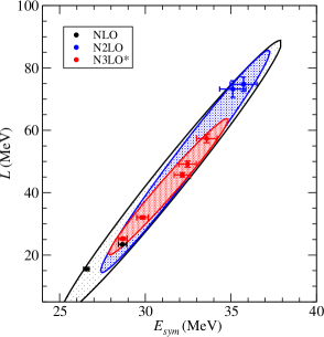
Figure 12: Adapted from Refs. Holt and Kaiser (2017); Drischler et al. (2021a). Left: Correlation between the symmetry energy $E_{sym}$ and its slope, $L$ at saturation, from $\chi$EFT calculations at different orders in the chiral expansion Holt and Kaiser (2017). Right: Microscopic constraints on the $E_{sym}-L$ correlation from Refs. Hebeler et al. (2010); Gandolfi et al. (2012); Holt and Kaiser (2017); Drischler et al. (2020).

Chiral effective field theory has also been employed to study the liquid-gas phase transition and thermodynamic EoS at low temperatures ($T<25$ MeV) in isospin-symmetric nuclear matter Wellenhofer et al. (2014). The EoS has been computed using $\chi$EFT nuclear potentials at resolution scales of 414, 450, and 500 MeV. The results from this study are tabulated in Table 3. In particular, the values of the liquid-gas critical endpoint in temperature, pressure, and density agree well with the empirical multifragmentation and compound nuclear decay experiments discussed in section VII.3. In addition, at low densities and moderate temperatures, the pure neutron matter EoS is well described within the virial expansion in terms of neutron-neutron scattering phase shifts. The results from chiral effective field theory have been shown Wellenhofer et al. (2015) to be in very good agreement with the model-independent virial EoS. Since finite-temperature effects are difficult to reliably extract empirically, chiral effective field theory calculations have been used to constrain the temperature dependence of the dense-matter EoS in recent tabulations Du et al. (2019, 2022) for astrophysical simulations.

Table 3: The N$3$LO contributions for binding energy per nucleon at saturation, saturation density, compressibility at saturation, and liquid-gas phase-transition critical values of temperature, density, and pressure at different resolution scales Wellenhofer et al. (2014).

.

Resolution scale	$\frac{B}{A}$(MeV)	$n_{sat}\left(\mathrm{fm}^{-3}\right)$	$K(\mathrm{MeV})$	$T_{c}(\mathrm{MeV})$	$n_{c}\left(\mathrm{fm}^{-3}\right)$	$P_{c}\left(\mathrm{MeV}\mathrm{fm}^{-3}\right)$
$414\left(M^{*}/M\right)$	$-15.79$	$0.171$	223	$17.4$	$0.066$	$0.33$
450 $\left(M^{*}/M\right)$	$-15.50$	$0.161$	244	$17.2$	$0.064$	$0.32$
500 $\left(\mathrm{no}~{}\mathrm{M}^{*}/M\right)$	$-16.51$	$0.174$	250	$19.1$	$0.072$	$0.42$

VI Experimental Constraints: Heavy-Ion Collisions

Given that hot and dense matter can be created experimentally in heavy-ion collisions, constraints on its EoS can be extracted via experimental measurements obtained from such collisions. As explained previously in subsection II.5, we will especially focus in this paper on the data themselves, and avoid citing quantities inferred from the data, as the latter come with an associated model dependence. We will mention particle production yields and their ratios, as well as fluctuation observables of particle multiplicities. Then, we will review experimental results on flow harmonics, to end with Hanbury-Brown-Twiss (HBT) interferometry measurements, also referred to in the field as femtoscopy.

We remind the reader that, as a general rule of thumb, high center of mass energy collisions, $\sqrt{s_{NN}}\gtrsim 200$ GeV, are in the regime of the phase diagram where $\mu_{B}\ll T$, such that the numbers of particles and anti-particles are approximately equal (i.e., $n_{B}\sim 0$). As one lowers $\sqrt{s_{NN}}$, baryons are stopped within the collision such that higher $n_{B}$ is reached. At sufficiently low beam energies, $\sqrt{s_{NN}}\lesssim 4-7$ GeV, matter is dominated by the hadron gas phase, such that lowering $\sqrt{s_{NN}}$ leads to lower temperatures and lower $n_{B}$.

VI.1 Particle yields

Particle production spectra are part of the simplest experimental observables used in heavy-ion collisions, to access thermodynamic properties and characteristics of the hot and dense matter. Starting with the integrated production yields of identified hadrons, they can be measured to help determine properties from the evolution of the system, in particular at chemical and kinetic freeze-out. These steps designate the ending of inelastic collisions between formed hadrons (what fixes the chemistry of the system) and in turn the ceasing of all elastic collisions (after which particles stream freely to the detectors) in the evolution of a heavy-ion collision. Statistical hadronization models Hagedorn (1965); Dashen et al. (1969); Becattini and Passaleva (2002); Wheaton et al. (2011); Petran et al. (2014); Andronic et al. (2018, 2019); Vovchenko and Stoecker (2019) are fitted to these yields and ratios by varying over $T$ and $\mu_{B}$, in order to extract the respective chemical freeze-out values. Despite their ability to reproduce particle yields successfully, those models are limited in scope since they do not reproduce the dynamics of a collision and hinge on the assumption of thermal equilibrium, which is not necessarily achieved within the short time scales of heavy-ion collisions. Similar information can also be inferred for kinetic freeze-out, using a so-called blast-wave model Schnedermann et al. (1993). The data from low transverse momentum particles (i.e., $p_{T}\lesssim 2-3$ GeV/c) measured at mid-rapidity (approximately transverse to the beam line direction) is used for statistical hadronization fits, because these particles spend the longest time within the medium (so they are more likely to be thermalized) and they have low enough momentum to avoid contributions from jet physics.

Measurement of yields for the most common light hadron species (namely $\pi^{\pm}$, $K^{\pm}$, $p/\overline{p}$) and strange hadrons ($\Lambda/\overline{\Lambda}$, $\Xi^{-}/\overline{\Xi}^{+}$ and $\Omega^{-}/\overline{\Omega}^{+}$) was achieved by STAR at RHIC and ALICE at the LHC. As part of the BES program, STAR has measured these hadron yields in Au+Au collisions at center-of-mass energies of $\sqrt{s_{NN}}=$7.7, 11.5, 14.5, 19.6, 27, 39, 62.4 and 200 GeV Abelev et al. (2009); Adamczyk et al. (2017); Adam et al. (2020a, b) and in U+U collisions at $\sqrt{s_{NN}}=193$ GeV Abdallah et al. (2023b). Motivated by results from the past SPS-experiment NA49 obtained from Pb+Pb collisions at $\sqrt{s_{NN}}<20$ GeV Alt et al. (2008), the NA61/SHINE experiment at CERN has conducted a scan in system-size and energy (in the same energy range as NA49). The diagram of all collided systems as a function of collision energy and nuclei is displayed in the left panel of Fig. 13. They published data for light hadrons in Ar+Sc Acharya et al. (2021a) and Be+Be collisions Acharya et al. (2021b) so far, while results from Xe+La and Pb+Pb collisions should become available in the next few years Kowalski (2022). At LHC energies, the higher $\sqrt{s_{NN}}$ produces significantly more particles, allowing more precise measurements of the species. For this reason, the ALICE experiment has measured yields not only for light and (multi)strange hadrons, but also for light nuclei and hyper-nuclei, in Pb+Pb collisions at 2.76 TeV/A in particular Abelev et al. (2013a, b, 2014a); Adam et al. (2016a); Acharya et al. (2018a); Adam et al. (2016b), and more recently in Pb+Pb collisions at 5.02 TeV/A too Acharya et al. (2020b); ALI (2022a), as well as Xe+Xe collisions at 5.44 TeV/A Acharya et al. (2021c).

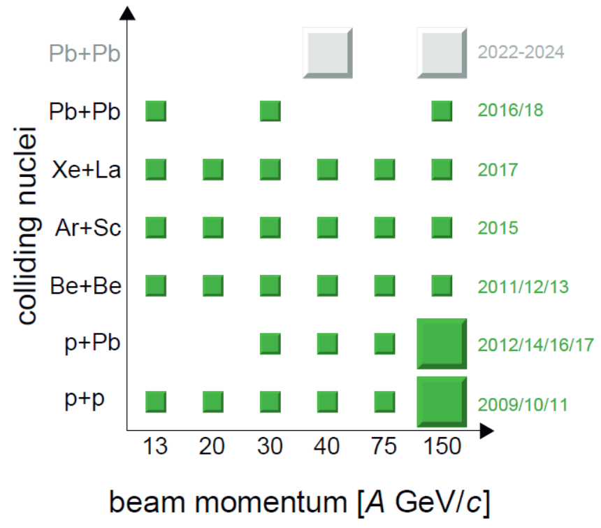
Figure 13: Left: diagram of different collided systems as a function of collision energy, from Ref. Kowalski (2022). Right: yields of hadrons measured by STAR in central Au+Au collisions at 7.7 and 39 GeV/A, compared with results from a grand canonical statistical hadronization model, from Ref. Acharya et al. (2018a).

The yields of particle production can also be used as an indicator of the onset of deconfinement, notably thanks to the strangeness enhancement: strange quark-antiquark pairs are expected to be produced at a much higher rate in a hot and dense medium than in a hadron gas. Hence, one should expect in particular an increase of multi-strange baryons compared to light-quark-compound hadrons in collision systems where the QGP has been formed, which has been observed experimentally in heavy-ion collisions at several energies Antinori et al. (2006); Abelev et al. (2008a, 2014a). Moreover, the distinctive non-monotonic behavior of the $K^{+}/\pi^{+}$ ratio as a function of the collision energy can also be considered as a sign of the onset of deconfinement, according to some authors Gazdzicki and Gorenstein (1999); Poberezhnyuk et al. (2015). This so-called “horn” in the $K^{+}/\pi^{+}$ ratio has been notably observed in Pb+Pb Afanasiev et al. (2002); Alt et al. (2008) and Au+Au collisions Akiba et al. (1996); Ahle et al. (2000); Abelev et al. (2009, 2010a); Adamczyk et al. (2017), but absent from p+p data Aduszkiewicz et al. (2017); Abelev et al. (2010a); Aamodt et al. (2011a); Abelev et al. (2014b) and Be+Be collisions results Acharya et al. (2021b). Recent results from Ar+Sc collisions Kowalski (2022) have, however, stirred up doubts regarding the interpretation of this observable, as the value of this ratio from such collision system is closer to the one measured in big systems, while no horn structure is seen, similar to small systems. All these results for different systems can be seen in Fig. 14.

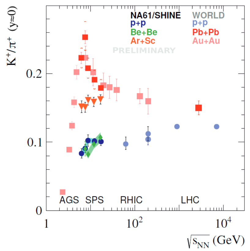
Figure 14: From Ref. Kowalski (2022). Preliminary results for the ratio of $K^{+}/\pi^{+}$ yields at mid-rapidity as a function of the collision energy, compared for different collision systems.

VI.2 Fluctuation observables

In heavy-ion collisions, observables measuring fluctuations are among the most relevant for the investigation of the QCD phase diagram. Within the assumption of thermodynamic equilibrium, cumulants of net-particle multiplicity distributions become directly related to thermodynamic susceptibilities, and can be compared to results from lattice QCD (see subsection III.2) to extract information on the chemical freeze-out line Alba et al. (2014, 2015, 2020). Moreover, large, relatively long-range fluctuations are expected in the neighborhood of the conjectured QCD critical point, making fluctuation observables very promising signatures of criticality Stephanov et al. (1999); Stephanov (2009); Athanasiou et al. (2010). It has also been proposed that the finite-size scaling of critical fluctuations could be employed to constrain the location of the critical point Palhares et al. (2011); Fraga et al. (2010); Lacey (2015); Lacey et al. (2016). In Fraga et al. (2010), finite-size scaling arguments were applied to mean transverse-momentum fluctuations measured by STAR Adams et al. (2005a, 2007) to exclude a critical point below $\mu_{B}\lesssim 450$ MeV.

Fluctuations of the conserved charges $B,S$, and $Q$ are of particular importance. As mentioned already in subsection III.2, these fluctuations can be used to probe the deconfinement transition, as well as the location of the critical endpoint. Calculated via the susceptibilities expressed in equation (3), which can be evaluated via lattice QCD simulations or HRG model calculations, they can also be related to the corresponding cumulants of conserved charges $C^{BSQ}_{lmn}$ , following the relation

$$C^{BSQ}_{lmn}=VT^{3}\times\chi^{BSQ}_{lmn}\ ,$$ (14)

with the volume $V$ and temperature $T$ of the system, and $l,m,n\in\mathbb{N}$ Luo and Xu (2017). The cumulants are also theoretically related to the correlation length of the system $\xi$, which is expected to diverge in the vicinity of the critical endpoint. In particular, the higher order cumulants are proportional to higher powers of $\xi$, making them more sensitive to critical fluctuations Stephanov et al. (1999); Stephanov (2009); Athanasiou et al. (2010).

In heavy-ion collisions, however, it is impossible to measure the fluctuations of conserved charges directly, because one cannot detect all produced particles (e.g., neutral particles are not always possible to measure, so that baryon number fluctuations do not include neutrons). Nevertheless, it is common to measure the cumulants of identified particles’ net-multiplicity distributions, using some hadronic species as proxies for conserved charges Koch et al. (2005). Net-proton distributions are used as a proxy for net-baryons Aggarwal et al. (2010); Adam et al. (2019a); Abdallah et al. (2021b), net-kaons Adamczyk et al. (2018a); Ohlson (2018); Adam et al. (2019b) or net-lambdas Adam et al. (2020c) are used as a proxy for net-strangeness, and net-pions+protons+kaons Adam et al. (2019b) has been recently used as a proxy for net-electric charge, instead of the actual net-charged unidentified hadron distributions. Mixed correlations have also been measured Adam et al. (2019b), although alternative ones have been suggested, that would provide more direct comparisons to lattice QCD susceptibilities Bellwied et al. (2020).

These net-particle cumulants can be used to construct ratios, as they are connected with usual statistic quantities characterizing the net-hadron distributions $N_{\alpha}=n_{\alpha}-n_{\overline{\alpha}}$ (with $n_{\alpha/\overline{\alpha}}$ being respectively the number of hadrons or anti-hadrons of hadronic specie $\alpha$). Hence, relations between such ratios and the mean $\mu_{\alpha}$, variance $\sigma_{\alpha}$, skewness $S_{\alpha}$ or kurtosis $\kappa_{\alpha}$ can be expressed as follows

$$\frac{\sigma_{\alpha}^{2}}{\mu_{\alpha}} =\frac{C_{2}^{\alpha}}{C_{1}^{\alpha}}=\frac{\langle(\delta N_{\alpha})^{2}\rangle}{\langle N_{\alpha}\rangle}\ ,$$ (15)

$$S_{\alpha}\sigma_{\alpha} =\frac{C_{3}^{\alpha}}{C_{2}^{\alpha}}=\frac{\langle(\delta N_{\alpha})^{3}\rangle}{\langle(\delta N_{\alpha})^{2}\rangle}\ ,$$ (16)

$$\kappa_{\alpha}\sigma_{\alpha}^{2} =\frac{C_{4}^{\alpha}}{C_{2}^{\alpha}}=\frac{\langle(\delta N_{\alpha})^{4}\rangle}{\langle(\delta N_{\alpha})^{2}\rangle}-3{\langle(\delta N_{\alpha})^{2}\rangle}\ ,$$ (17)

$$\frac{\kappa_{\alpha}\sigma_{\alpha}}{S_{\alpha}} =\frac{C_{4}^{\alpha}}{C_{3}^{\alpha}}=\frac{\langle(\delta N_{\alpha})^{4}\rangle-3{\langle(\delta N_{\alpha})^{2}\rangle}^{2}}{\langle(\delta N_{\alpha})^{3}\rangle}\ ,$$ (18)

with $\delta N_{\alpha}=N_{\alpha}-\langle N_{\alpha}\rangle$, and $\langle\,\rangle$ denoting an average over the number of events in a fixed centrality class at a specific beam energy Luo and Xu (2017). These ratios allow for more direct comparisons to theoretical calculations of susceptibilities because the leading order dependence on volume and temperature cancels out (see (14)).

While direct comparisons between theoretically calculated susceptibilities and multi-particle cumulants have been made, certain caveats exist. First of all, these comparisons are only valid if the chosen particle species are good proxies for their respective conserved charge (see e.g. Chatterjee et al. (2016); Bellwied et al. (2020)). Additionally, there are fundamental conceptual differences between the assumed in-equilibrium and infinite volume lattice QCD calculations on one side, and the highly dynamical, far-from-equilibrium, short-lived, and finite-size system created in heavy-ion collisions on the other side. While building cumulant ratios cancels the trivial dependence on volume and temperature, it does not prevent volume fluctuations that can affect the signal, especially for higher order cumulants Gorenstein and Gazdzicki (2011); Konchakovski et al. (2009); Skokov et al. (2013); Luo and Xu (2017). Calculating the cumulants as a function of the centrality class will generally increase the signal, as the volume of systems varies within a single centrality class Luo et al. (2013). Also known as the centrality bin-width effect, this artificial modification of the measured fluctuations can be minimized by using small centrality classes, and some correction methods Sahoo et al. (2013); Gorenstein (2015). A second consequence is the fact that the finite size of the system limits the growth of $\xi$. The correlation length must be smaller than the size of the system itself and $\xi$ is even smaller when the system is inhomogeneous Stephanov et al. (1999). Because the system only approaches the critical point for a finite period of time, the growth of $\xi$ would be consequently limited, restraining even more the size of measured fluctuations amplitude Berdnikov and Rajagopal (2000); Hippert et al. (2016); Herold et al. (2016). Critical lensing effects may somewhat compensate for some of these effects by drawing more of the system towards the critical regime Dore et al. (2022).

Finally, the width of the rapidity (angle with respect to the beam line) window in which particle cumulants are measured is important. The signal from critical fluctuations is expected to have a correlation range of $\Delta y\sim 1$, hence cumulants should be measured with particles in a rapidity of this order at least to be sensitive to criticality Ling and Stephanov (2016). Another alternative is to use factorial cumulants $\hat{C}_{n}$ (also referred to as correlation functions), which can be expressed as linear combinations of cumulants $C_{n}$ and are better suited for acceptance dependence studies because of their linear scaling with the rapidity acceptance Ling and Stephanov (2016); Bzdak et al. (2017). Moreover, acceptance cuts may also affect fluctuation observables and, together with detection efficiency effects, contribute with spurious binomial fluctuations Pruneau et al. (2002); Bzdak and Koch (2012); Garg et al. (2013); Karsch et al. (2016); Hippert and Fraga (2017). Resonance decays can also lead to spurious contributions, as has been discussed in Begun et al. (2006); Sahoo et al. (2013); Garg et al. (2013); Nahrgang et al. (2015); Bluhm et al. (2017); Mishra et al. (2016); Hippert and Fraga (2017).

VI.2.1 Net-$p$ fluctuations

Experimental collaborations commonly use the net-proton distribution as a proxy for the baryon number $B$, even though protons experience isospin randomization during the late stages of the collision Kitazawa and Asakawa (2012a); Nahrgang et al. (2015). This process causes the original nucleon isospin distribution to be blurred and is due to the reactions $p+\pi^{0/-}\leftrightarrow\Delta^{+/0}\leftrightarrow n+\pi^{+/0}$ that nucleons undergo several times during the hadronic cascade. These reactions do not affect net-$B$ fluctuations, but do affect net-proton fluctuations. Since protons are the only nucleons measured in the final state, isospin randomization has to be taken into account when comparing both quantities Kitazawa and Asakawa (2012b).

The ALICE collaboration has published measurements of $C_{1}^{p}$ and $C_{2}^{p}$ net-proton cumulants and their ratios in Pb+Pb collisions at $\sqrt{s_{NN}}=2.76$ TeV Acharya et al. (2020a) and at $\sqrt{s_{NN}}=5.02$ TeV $C_{3}^{p}$ was also measured ALI (2022b). As the system is created at almost vanishing baryonic chemical potential at such high energies, those cumulants can be compared to lattice QCD susceptibility results like the one discussed in subsection III.2, keeping in mind the subtleties of such comparison mentioned in the previous paragraph. However, no critical signal is expected in such collisions, they are mostly used to study correlation dynamics and the effect of global and local charge conservation ALI (2022c). Only higher-order cumulants, from $C^{p}_{6}$ and beyond, are expected to exhibit $O(4)$ criticality Friman et al. (2011); Almasi et al. (2019). At RHIC energies, the STAR experiment has measured net-proton (factorial) cumulants as one of the main objectives of the BES program, in Au+Au collisions from $\sqrt{s_{NN}}=200$ GeV down to $\sqrt{s_{NN}}=7.7$ GeV for cumulants up to $C^{p}_{4}$, and even down to $\sqrt{s_{NN}}=3$ GeV for up to $C^{p}_{6}$ Abdallah et al. (2021b); Aboona et al. (2023). One of the most interesting results is the energy dependence of the $C^{p}_{4}/C^{p}_{2}$ ratio, shown in the left panel of Fig. 15, which exhibits a non-monotonic behavior with a significance of $3.1\sigma$ towards low collision energies Abdallah et al. (2021b). The right panel of Fig. 15 shows a theoretical calculation of one possible critical point from Stephanov (2011) using a 3D Ising model. Such non-monotonic behavior of the net-proton kurtosis, and more specifically the peak arising after the dip when going to lower energy, had been predicted as an effective sign of the existence a critical region in the phase diagram in Ref. Stephanov (2011) (later work Mroczek et al. (2021, 2022) has found exceptions to this using the same framework but incorporating all higher order terms, demonstrating that the peak in kurtosis is the most important signal for the critical point but the bump is not always present). Further investigations are already planned to enlighten this special result, by collecting more data in low-energy collisions and especially exploring energies below $\sqrt{s_{NN}}=7.7$ GeV in the BES-II program Tlusty (2018). They will complete the results of the HADES collaboration, which published a complete analysis for net-$p$ cumulants up to $C^{p}_{4}$, in Au+Au collisions at $\sqrt{s_{NN}}=2.4$ GeV Adamczewski-Musch et al. (2020a).

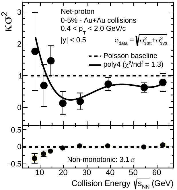
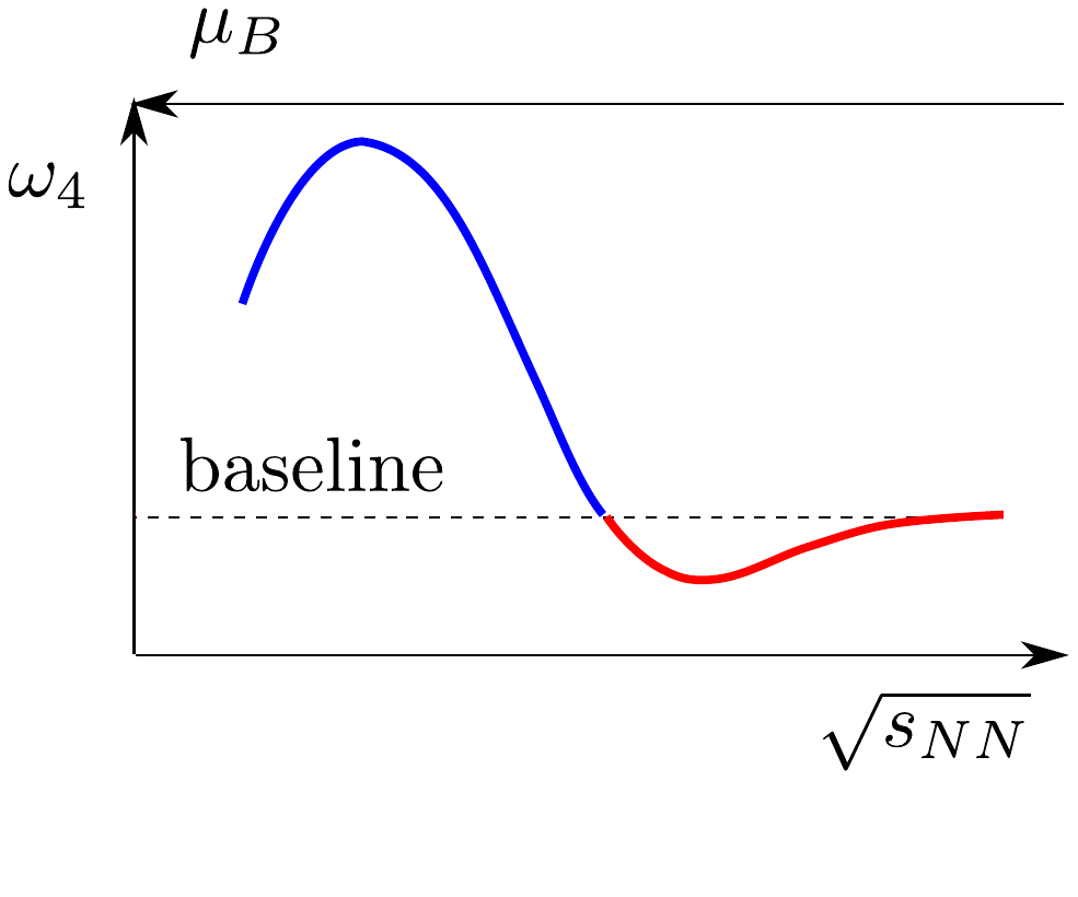
Figure 15: Left: energy dependence of the $C_{4}/C_{2}(=\kappa\sigma^{2})$ ratio from net-$p$ distribution for $|y|<0.5$ and $0.4<p_{T}<2.0$ GeV/c, measured in $0-5\%$ Au-Au collisions by the STAR collaboration, from Ref. Abdallah et al. (2021b). Right: expected behavior of the $C_{4}/C_{1}(=\omega_{4})$ ratio for net-$p$, in the case of a freeze-out line passing through the critical region near the critical endpoint, from Ref. Bzdak et al. (2020).

VI.2.2 Net-charged hadron fluctuations

Electric charge fluctuations are the easiest to measure experimentally, as charged particle distributions are accessible even without having to identify the detected particles. Both STAR Adamczyk et al. (2014a) and PHENIX Adare et al. (2016a) collaborations have published results of net-$Q$ cumulants up to $C_{4}^{Q}$ in Au+Au collisions from 7.7 to 200 GeV/A, shown for PHENIX in Fig. 16, with no evidence of a peak that could hint at the presence of a critical endpoint. The same net-$Q$ cumulants have also been measured by the NA61/SHINE experiment in smaller systems (Be+Be and Ar+Sc) for several collision energies within $5.1\leq\sqrt{s_{NN}}\leq 17.3$ GeV, without any sign of criticality Marcinek (2023). Combining net-p and net-Q fluctuations can be used to extract the $T,\mu_{B}$ at freeze-out for a specific $\sqrt{s_{NN}}$ and centrality class (normally central collisions of 0-5%). This has been done within a hadron resonance gas model where acceptance cuts and isospin randomization can be taken into account Alba et al. (2014, 2015, 2020) but consistent results have also been found from lattice QCD susceptibilities as well Borsanyi et al. (2014b) that cannot take those effects into account.

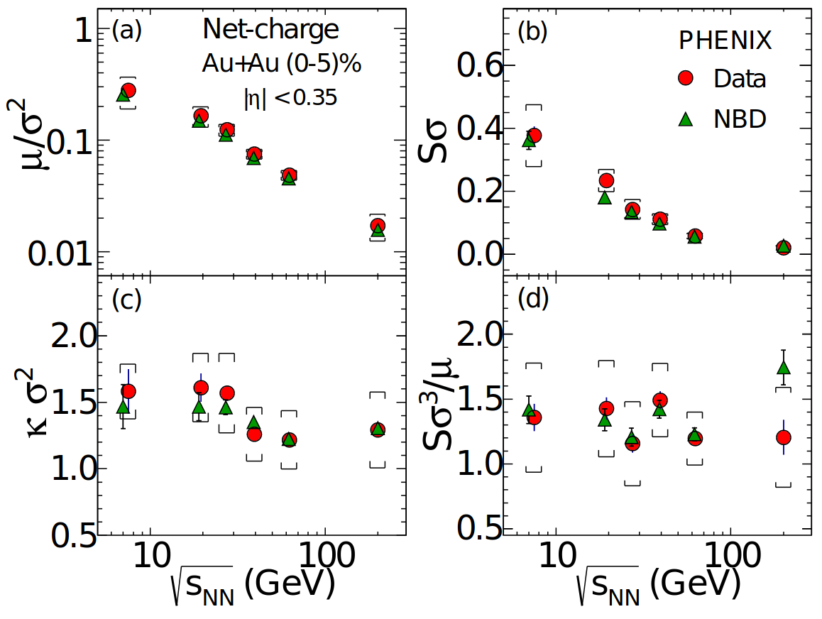
Figure 16: Energy dependence of $\mu/\sigma^{2}\sim C_{1}/C_{2}$, $S\sigma\sim C_{3}/C_{2}$, $\kappa\sigma^{2}\sim C_{4}/C_{2}$ and $S\sigma^{3}/\mu\sim C_{3}/C_{1}$ for net-$Q$ in central Au+Au collisions for particles with $0.3<p_{T}<2.0$ GeV and within $|\eta|<0.35$, from the PHENIX collaboration Adare et al. (2016a). Data are compared with negative binomial-distribution (NBD).

VI.2.3 Net-K, net-$\Lambda$ fluctuations

In the strangeness sector, net-kaon (specifically $K^{\pm}$) distributions are used as a proxy, since they are abundantly produced and easily reconstructed in heavy-ion collisions. Because all other strange particles carry baryon number, the resulting cumulants separated by particle species can provide varying results Zhou et al. (2017). These cumulants have been measured extensively by the STAR experiment, again in Au+Au collisions from 7.7 to 200 GeV/A up to $C^{K}_{4}$ Adamczyk et al. (2018a), see Fig. 17. The ALICE collaboration has also published some preliminary results of $C_{1}$ and $C_{2}$ for net-$K$ distributions, along with net-$\pi$ and net-$p$ results, in Pb+Pb collisions at 2.76 TeV/A Ohlson (2018). Recently, net-$\Lambda$ cumulants up to $C^{\Lambda}_{3}$ order and their ratios have also been measured by the STAR experiment, in Au+Au collisions at $\sqrt{s_{NN}}=19.6,27,39,62.4$ and 200 GeV Adam et al. (2020c). Note that $\Lambda$ results inherently include contamination from $\Sigma^{0}$ baryons, which decay with a branching ratios of 100% via the channel $\Sigma^{0}\to\Lambda+\gamma$ and cannot be discriminated from primary $\Lambda$ production. Such results on event-by-event fluctuations of $\Lambda$ baryons are important to investigate the interplay between baryon number and strangeness conservation at hadronization.

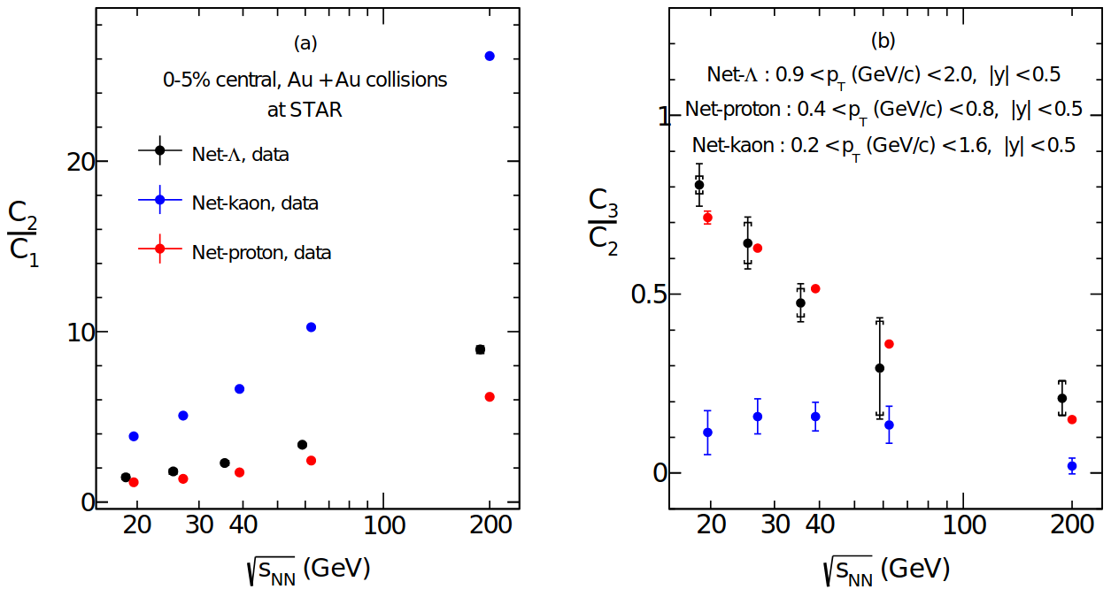
Figure 17: Energy dependence of $C_{2}/C_{1}$ and $C_{3}/C_{2}$ for net-$\Lambda$, net-$K$ and net-$p$ within $|y|<0.5$ in central Au+Au collisions, from the STAR collaboration Adam et al. (2020c).

It was proposed in Bellwied et al. (2013) from lattice QCD that there may be a flavor hierarchy wherein strange particles freeze-out at a higher temperature than light particles. The idea relies on the change in the degrees of freedom in comparisons between various lattice susceptibilities for light and strange quarks to the hadron resonance gas model. The original lattice QCD paper suggested strange particles hadronize at $T\sim 10-15$ MeV higher temperatures than light particles. Using the net-K and net-$\Lambda$ results, it has been shown from both a hadron resonance gas Bellwied et al. (2019); Bluhm and Nahrgang (2019) and lattice QCD Noronha-Hostler et al. (2016a) that a preference for a higher freeze-out temperature for strangeness is preferred (although the exact temperature is somewhat model dependent).

VI.2.4 Mixed conserved charges

In addition to the so-called “diagonal” cumulants, i.e., cumulants of net-multiplicity distribution for hadronic species related to a single conserved charge, the STAR collaboration measured off-diagonal cumulants that represent correlations between different conserved charges Koch et al. (2005); Majumder and Muller (2006). STAR extracted results for covariances, i.e. $C_{2}$ mixed-cumulants of net-$Q$, net-$p$, and net-$K$ distributions (proxies for $B$ and $S$ respectively) and their ratios, from Au+Au collisions in the usual BES-I collision energy range $7.7\leq\sqrt{s_{NN}}\leq 200$ GeV Adam et al. (2019b). The full suite of experimental observables was $\sigma^{1,1}_{Q,p}$, $\sigma^{1,1}_{Q,K}$, $\sigma^{1,1}_{Q,K}$, $\sigma^{1,1}_{Q,p}/\sigma^{2}_{p}$, $\sigma^{1,1}_{Q,K}/\sigma^{2}_{K}$, $\sigma^{1,1}_{p,K}/\sigma^{2}_{K}$. While both $\sigma^{1,1}_{Q,p}/\sigma^{2}_{p}$ and $\sigma^{1,1}_{Q,K}/\sigma^{2}_{K}$ ratios show only a small collision energy dependence and no peculiar behavior, the $\sigma^{1,1}_{p,K}/\sigma^{2}_{K}$ ratio exhibits a global sign change around $\sqrt{s_{NN}}\sim 20$ GeV, as can be seen in Fig. 18. Even though not straightforward to interpret, this result might provide important insight into the onset of deconfinement. In Bellwied et al. (2020) it was argued that the current off-diagonal cumulants were not the best to reproduce lattice QCD due to “missing” hadrons that could not be measured experimentally (e.g. neutrons). Thus, it was suggested to instead measure $\sigma^{2}_{\Lambda}/\left(\sigma^{2}_{K}+\sigma^{2}_{\Lambda}\right)$ and $\sigma^{2}_{K}/2\left(\sigma^{2}_{\Lambda}+\sigma^{2}_{K}\right)$ to assess, respectively, strange baryon correlations and strange electric charge correlations. These can be reconstructed using the data from Adam et al. (2020b) and Adam et al. (2020c).

Figure 18: From Ref. Adam et al. (2019b). Centrality dependence of covariance to variance ratios for net-$Q$, net-$p$, and net-$K$ distributions in Au+Au collisions at different collision energies from the STAR collaboration, compared with results from ultra-relativistic quantum molecular dynamics (UrQMD) simulations.

VI.2.5 Summary of cumulant observables for conserved charge proxies

In terms of theoretical comparisons to these data points, each theoretical approach has its own caveats. In principle, lattice QCD only provides results for the infinite volume limit, it cannot account for decays, cannot account for limited particle species (i.e. effects like isospin randomization are missed), nor can it account for kinematic cuts. However, using partial pressures Noronha-Hostler et al. (2016a) it is at least possible to capture fluctuations of certain hadronic species (i.e. kaons) more directly from lattice QCD. A hadron resonance gas approach does have the advantage of fitting lattice QCD very well at temperatures below $T\sim 150-165$ MeV (the exact temperature depends on the observable), can take into account isospin randomization and kinematic cuts, and can calculate quantities for specific particle species. However, a hadron resonance gas model is dependent on the particle list considered (incomplete particle lists can lead to misleading results) and cannot take into account dynamical effects or out-of-equilibrium effects. A third option is also often used, which are hadron transport codes like UrQMD Bass et al. (1998); Bleicher et al. (1999) or SMASH Weil et al. (2016); Hammelmann and Elfner (2022) that can take into account all the dynamical and out-of-equilibrium effects. However, transport models have the caveats that they cannot take into account decays and interactions of more than 2 bodies (i.e. $1\rightarrow 3$ body decays are excluded, even though they are known to exist experimentally) and their connection to temperature is more tenuous.

In Table 4 we summarize the latest results from ALICE, STAR, HADES, and NA61/SHINE on all the cumulants for net-proton, net-charge, and net-strangeness. We note that new results are anticipated later this year from STAR’s Beam Energy Scan II program that will significantly reduce the error bars from BES I and also provide new beam energies in the fixed target regime i.e. between $\sqrt{s_{NN}}=3-7.7$ GeV.

Cumulant ratio	System	Experiment	$\sqrt{s_{NN}}$
$C^{p}_{2}/C^{p}_{1}$	Au+Au	HADES Adamczewski-Musch et al. (2020a)	2.4 GeV
		STAR Abdallah et al. (2021b)	7.7, 11.5, 14.5, 19.6, 27, 39, 54.4, 62.4, 200 GeV
$C^{p}_{2}/\langle p+\bar{p}\rangle$	Pb+Pb	ALICE Acharya et al. (2020a); ALI (2022b)	2.76, 5.02 TeV
$C^{p}_{3}/C^{p}_{1}$	Au+Au	PHENIX Adare et al. (2016a)	7.7, 19.6, 27, 39, 62.4, 200 GeV
$C^{p}_{3}/C^{p}_{2}$	Au+Au	HADES Adamczewski-Musch et al. (2020a)	2.4 GeV
		STAR Abdallah et al. (2021b)	7.7, 11.5, 14.5, 19.6, 27, 39, 54.4, 62.4, 200 GeV
$C^{p}_{4}/C^{p}_{2}$	Au+Au	HADES Adamczewski-Musch et al. (2020a)	2.4 GeV
		STAR Aboona et al. (2023); Abdallah et al. (2021b)	3, 7.7, 11.5, 14.5, 19.6, 27, 39, 54.4, 62.4, 200 GeV
$C^{p}_{5}/C^{p}_{1}$	Au+Au	STAR Aboona et al. (2023)	3, 7.7, 11.5, 14.5, 19.6, 27, 39, 54.4, 62.4, 200 GeV
$C^{p}_{6}/C^{p}_{2}$	Au+Au	STAR Aboona et al. (2023)	3, 7.7, 11.5, 14.5, 19.6, 27, 39, 54.4, 62.4, 200 GeV
$C^{Q}_{2}/C^{Q}_{1}$	Au+Au	PHENIX Adare et al. (2016a)	7.7, 19.6, 27, 39, 62.4, 200 GeV
	Au+Au	STAR Adamczyk et al. (2014a)	7.7, 11.5, 19.6, 27, 39, 62.4, 200 GeV
$C^{Q}_{3}/C^{Q}_{1}$	Au+Au	PHENIX Adare et al. (2016a)	7.7, 19.6, 27, 39, 62.4, 200 GeV
$C^{Q}_{3}/C^{Q}_{2}$	Au+Au	PHENIX Adare et al. (2016a)	7.7, 19.6, 27, 39, 62.4, 200 GeV
		STAR Adamczyk et al. (2014a)	7.7, 11.5, 19.6, 27, 39, 62.4, 200 GeV
$C^{Q}_{4}/C^{Q}_{2}$	Au+Au	PHENIX Adare et al. (2016a)	7.7, 19.6, 27, 39, 62.4, 200 GeV
		STAR Adamczyk et al. (2014a)	7.7, 11.5, 19.6, 27, 39, 62.4, 200 GeV
$C^{K}_{2}/C^{K}_{1}$		STAR Adamczyk et al. (2018a)	7.7, 11.5, 14.5, 19.6, 27, 39, 62.4, 200 GeV
$C^{K}_{3}/C^{K}_{2}$		STAR Adamczyk et al. (2018a)	7.7, 11.5, 14.5, 19.6, 27, 39, 62.4, 200 GeV
$C^{K}_{4}/C^{K}_{2}$		STAR Adamczyk et al. (2018a)	7.7, 11.5, 14.5, 19.6, 27, 39, 62.4, 200 GeV
$C^{\Lambda}_{2}/C^{\Lambda}_{1}$		STAR Adam et al. (2020c)	19.6, 27, 39, 62.4, 200 GeV
$C^{\Lambda}_{3}/C^{\Lambda}_{2}$		STAR Adam et al. (2020c)	19.6, 27, 39, 62.4, 200 GeV

Table 4: Summary of cumulant ratios of different particle species for which measurements have been published by experiments across several collision energies ($\sqrt{s_{NN}}$) and systems.

VI.2.6 Other types of fluctuations

Other observables used to study two-particle correlations are the dynamical fluctuations, $\nu_{\text{dyn}}$, which can be used in the case of incomplete particle detection, even though $\nu_{\text{dyn}}$ intrinsically depends on multiplicity Gavin and Kapusta (2002); Pruneau et al. (2002). Two-species correlations between proton, kaon, and pion distributions have been investigated by the NA49, STAR, and ALICE collaborations, in very central Pb+Pb and Au+Au collisions for $6.3\leq\sqrt{s_{NN}}\leq 17.3$ GeV, $7.7\leq\sqrt{s_{NN}}\leq 200$ GeV and $\sqrt{s_{NN}}=2.76$ TeV, respectively Anticic et al. (2014); Abdelwahab et al. (2015); Acharya et al. (2019a). The energy dependence of $\nu_{\text{dyn}}[\pi,K]$ and $\nu_{\text{dyn}}[p,K]$ from NA49 data, in particular, displays a strong variation below center-of-mass energy $\sqrt{s_{NN}}\sim 10$ GeV, as can be seen in Fig. 19. This could indicate a change in the production mechanism of such particles, hinting at differences in the phases probed in these collisions Acharya et al. (2019a). The ALICE collaboration recently presented preliminary results on the system-size dependence of $\nu_{\text{dyn}}[+,-]$ normalized by charged particle density to remove its intrinsic multiplicity dependence. The data collected from p+p, p+Pb, and Pb+Pb collisions at $\sqrt{s_{NN}}=5.02$ TeV, and Xe+Xe collisions at $\sqrt{s_{NN}}=5.44$ TeV display a decreasing trend with the size of collided systems that no model has been able to completely reproduce Sputowska (2022).

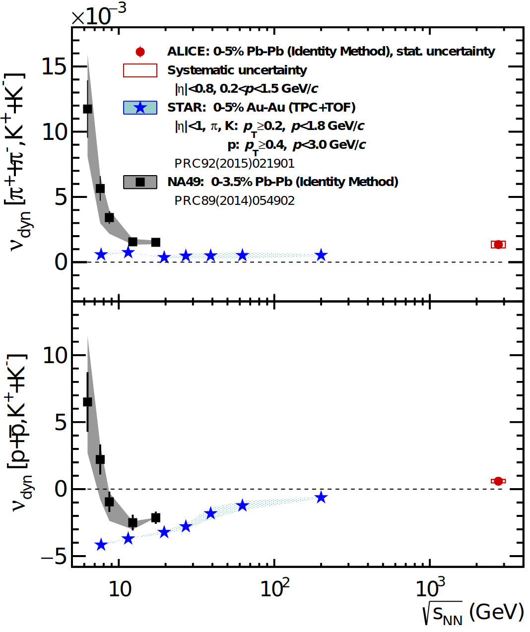
Figure 19: Combined results from STAR measurements in central Au+Au collisions, and ALICE and NA49 measurements in central Pb+Pb collisions on the energy dependence of $\nu_{\text{dyn}}[\pi,K]$ and $\nu_{\text{dyn}}[p,K]$ Acharya et al. (2019a).

Intensive and strongly intensive quantities can be used to investigate hadron number fluctuations, getting rid of the volume dependence and volume fluctuations, as proposed in Ref. Gorenstein and Gazdzicki (2011). Some of the results introduced earlier, like the scaled cumulants published by ALICE in ALI (2022b), STAR in Abdallah et al. (2021b) or NA61/SHINE in Marcinek (2023) are in fact intensive quantities by construction.

Scaled factorial moments $F_{r}(M)$ of order $r$ can be used to study the presence of the critical endpoint or phase transition, as they are defined to be sensitive to large multiplicity fluctuations caused by criticality Bialas and Peschanski (1986); Satz (1989); Bialas and Hwa (1991). They are defined as

$$F_{r}(M)=\frac{\left\langle\frac{1}{M^{D}}\sum^{M^{D}}_{i=1}n_{i}(n_{i}-1)...(n_{i}-q+1)\right\rangle}{\left\langle\frac{1}{M^{D}}\sum^{M^{D}}_{i=1}n_{i}\right\rangle^{q}}\ ,$$ (19)

with $M^{D}$ the number of bins in which the $D$-dimensional momentum space is partitioned, $n_{i}$ the multiplicity of particles of interest in the $i^{\text{th}}$ bin, and $r$ the order of the moment of interest Wu et al. (2020). The NA61/SHINE collaboration has measured $F_{2}(M)$ for protons in central Pb+Pb and Ar+Sc collisions, and $F_{2,3,4}(M)$ for negatively charged hadrons at several energies below $\sqrt{s_{NN}}=17$ GeV, showing no signal of any criticality in such systems Adhikary (2022).

Fluctuations of the mean transverse momentum, as those of conserved quantities, would also diverge at the critical point in equilibrium and are expected to be enlarged in its vicinity Stephanov et al. (1999). Mean transverse momentum correlations have been measured by the STAR collaboration, for beam energies of $\sqrt{s_{NN}}=20,62,130$ and $200$ GeV Adams et al. (2005a, 2007).

VI.3 Flow harmonics

Another important class of observables giving information about the dynamics of heavy-ion collisions and the EoS of nuclear matter are the flow harmonics $v_{n}$. They are the coefficients of the Fourier expansion of an $N$-particle triple-differential distribution

$$E\frac{d^{3}N}{d^{3}p}=\frac{1}{2\pi}.\frac{d^{2}N}{p_{T}dp_{T}dy}\left(1+2\sum_{n=1}^{\infty}v_{n}.\cos{(n(\phi-\Psi))}\right)\ ,$$ (20)

where $E$ is the particle energy, $p_{(T)}$ its (transverse) momentum, $y$ its rapidity, $\phi$ its azimuthal angle and $\Psi$ the event plane angle. The flow coefficients are defined as $v_{n}=\langle\cos(n(\phi-\Psi))\rangle$, $\langle...\rangle$ denoting an average over many collision events Voloshin and Zhang (1996); Poskanzer and Voloshin (1998). These flow coefficients measure the azimuthal anisotropies of particle distributions and are a signature of collective expansion, with $v_{2}$ measurements playing an important role in the conclusion that QGP formation was observed in Au+Au collisions at RHIC Adcox et al. (2005); Back et al. (2005a); Adams et al. (2005b).

VI.3.1 Measuring collective flow across $\sqrt{s_{NN}}$: event-plane vs multi-particle cumlant methods

While collective flow harmonics may initially appear deceptively simple as just a $\cos$ term, there are a number of subtle details that the reader must be aware of before making direct theory-to-experiment comparisons. There are two primary methods used to calculate $v_{n}$ for low $p_{T}$ particles (for the relevance to the EoS we will focus only on low $p_{T}$ particles but at high $p_{T}$ other technical details exist both on the theory and experimental side, some of which are discussed in Betz et al. (2017)). Before explaining the two methods, it is important to first understand that collective flow is not just a scalar quantity but rather it is a vector that contains both the magnitude of the flow $v_{n}$ that is 0 for a circular event and 1 for the extreme of the corresponding shape (i.e. for elliptical flow, $v_{2}$, it would appear as a line) and the corresponding event-plane angle $\Psi_{n}$ that is the direction of the flow vector. Then, the flow harmonic can be defined as the complex vector

$$V_{n}=v_{n}e^{in\Psi_{n}}\ .$$ (21)

To be clear, $\Psi_{n}$ is the event plane angle reconstructed by the detector that includes all the usual caveats of having finite number of particles, acceptance cuts, and efficiencies. However, in principle, if all particles were measured to infinite precision one could rigorously define the underlying event plane $\Phi_{n}$ that is the actual event plane of the given event. Due to the previously mentioned detector effects, $\Psi_{n}\neq\Phi_{n}$ and the dispersion in this relationship can be defined as the resolution, $R,$ for a specific flow harmonic

$$R\left(v_{n}\right)\equiv\langle e^{in\left(\Psi_{n}-\Phi_{n}\right)}\rangle\ ,$$ (22)

wherein the bracket $\langle\dots\rangle$ indicates an averaging over a large ensemble of events.

At this point, we can discuss the two different methods for calculating flow harmonics. The first one is the “event plane method” Poskanzer and Voloshin (1998), which was the first technique used to calculate flow harmonics. At that time it was assumed that dynamical fluctuations would have a negligible effect on the extraction of the event plane, such that $v_{n}$ would essentially be the same for all events within a fixed centrality class. In this method, $\Psi_{n}$ is determined from two or more subsets of particles (A and B, known as subevents) within a single event such that

$$\psi_{n}^{A,B}\equiv\frac{1}{n}\frac{\sum_{i\in A,B}w_{i}\sin\left(n\phi_{i}\right)}{\sum_{i\in A,B}w_{i}\cos\left(n\phi_{i}\right)}\ ,$$ (23)

where $n$ is the number of particles considered and $w_{i}$ is a relevant weight (such as energy or momentum). At this point, it is important to discuss the type of particles considered. The most standard flow measurements are all charged particles. However, it can be of interest to study the flow of identified particles such as protons, pions, or kaons. In that case, one “particle of interest”, subevent A, is taken (e.g. kaons) and one “reference particle”, subevent B, is taken from all charged particles. Because particles of interest tend to be rarer, in most cases only one particle of interest is considered rather than 2 (although exceptions exist). Next, the flow harmonic is determined via

$$v_{n}\left\{EP\right\}\equiv\frac{\langle\cos\left(\phi_{n}-\Psi_{n}^{A}\right)\rangle_{poi}}{\sqrt{\langle\cos\left(\phi_{n}-\Psi_{n}^{A}\right)\rangle}_{all}}\ ,$$ (24)

where the average in the numerator is only of particle of interest and the average in the denominator is over all charged particles.

The second method is the “multi-particle cumulant” method Borghini et al. (2001a); Bilandzic et al. (2011, 2014) that correlates $m$ number of particles. In this method (here we follow the formalism used in Luzum and Petersen (2014)) one can correlate $m$ particles such that

$$\langle m\rangle_{n_{1},n_{2},\dots,n_{m}}\equiv\langle\langle\cos\left(n_{1}\phi^{a_{1}}+n_{2}\phi^{a_{2}}+\dots+n_{m}\phi^{a_{m}}\right)\rangle_{m}\rangle_{ev}\ ,$$ (25)

where averages over particles are indicated by the subscript $m$ and averages over events are indicated by a subscript $ev$. While not shown here, often these averages also include weights (such as by multiplicity) when averaging over multiple events (we will revisit this concept later). At this point we should note that Eq. (25) leads to two distinct contributions that are flow $v_{n}$ (single particle distribution) and non-flow $\delta_{n,p}$ (genuine $p$-particle correlations that arise from things like a $\rho\rightarrow\pi\pi$ decay). Because hydrodynamics leads to only flow, experimentalists use various methods to minimize non-flow in their data analysis. Returning to Eq. (25), a 2-particle correlation of all charged particles (i.e. with no particle of interest) leads to

$$v_{n}\left\{2\right\}\equiv\sqrt{\langle v_{n}^{2}\rangle_{ev}+\langle\delta_{2,2}\rangle_{ev}}\ ,$$ (26)

where one gets a contribution both from genuine flow and 2-particle correlations. In order to minimize the non-flow contribution, rapidity gaps are taken within the experiments. They remove decay and jet effects that occur close to each other in rapidity. Thus, after these cuts it is reasonable to assume that

$$v_{n}\left\{2\right\}\approx\sqrt{\langle v_{n}^{2}\rangle_{ev}}\ ,$$ (27)

such that in theoretical calculations one can directly calculate $v_{n}$ for a single event and then take the root-mean-squared over many events to calculate $v_{n}\left\{2\right\}$. Notice that event-by-event flow fluctuations will also contribute to Eq. (27) and to multi-particle cumulants in general, and should be taken into account when comparing to hydrodynamic simulations.

Depending if one is in a high resolution limit (i.e. $v_{n}\gg 1/\sqrt{N}$ and $R\rightarrow 1$) or the low resolution limit (i.e. $v_{n}\sqrt{N}\ll 1$ and $R\rightarrow v_{n}\sqrt{N}$) the correct theoretical quantity to calculate varies Luzum and Ollitrault (2013) such that

$$v_{n}\left\{EP\right\} \xrightarrow[\text{high res}]{} \langle v_{n}\rangle\ ,$$ (28)

$$v_{n}\left\{EP\right\} \xrightarrow[\text{low res}]{} \sqrt{\langle v_{n}^{2}\rangle}\ .$$ (29)

However, most calculations fall between the high and low resolution limits, leading to ambiguous comparisons to experimental data. Thus, only the multi-particle cumulant method that explicitly defines a two particle correlation as

$$v_{n}\left\{2\right\}\equiv\sqrt{\langle v_{n}^{2}\rangle}\ ,$$ (30)

provides a method for unambiguous comparisons between theory and experiment.

Due to these uncertainties in the comparison between theory and experiment, only the multi-particle cumulant method ensures an apples-to-apples comparison Luzum and Ollitrault (2013). However, currently multi-particle cumulants have not been adopted uniformly across $\sqrt{s_{NN}}$ but rather, at low energies the event-plane method is still used and at high-energies multi-particle cumulants are the standard. As explained in Luzum and Ollitrault (2013), this may lead to just a difference of few percentage points in the results, but for precision calculations that can lead to ambiguities.

An additional caveat when comparing high and low beam energies is the choice of event plane angle that is used in the experimental analysis. At high $\sqrt{s_{NN}}$, in the rare occasions in which the event-plane angle is used, the latter is always consistent with the flow harmonic such that $v_{2}$ is measured with $\Psi_{2}$, $v_{3}$ is measured with $\Psi_{3}$ and so on. However, at low beam energies all collective flow harmonics are measured with the event-plane method, relative to spectator reaction plane, $\Psi_{1}$ Reisdorf et al. (2012). Thus, the interpretation of the flow harmonics is quite different than those measured at high $\sqrt{s_{NN}}$. At the time of writing, we are not aware of a systematic study within a theoretical model comparing the differences between these measurements across $\sqrt{s_{NN}}$. However, experiments have compared these methods and found differences between them Bastid et al. (2005); Aamodt et al. (2011b).

Other caveats exist when comparing theory to experiment. The averaging over events, $\langle\dots\rangle_{ev}$ normally is weighted by a certain factor $W_{i}$ that is a function of the multiplicity, $M$, of a given event such that

$$\langle\dots\rangle_{ev}\equiv\frac{\sum_{i}^{ev}\langle\dots\rangle_{i}W_{i}}{\sum_{i}^{ev}W_{i}}\ ,$$ (31)

where for a two-particle correlation $W=M(M-1)$. The averaging in Eq. (31) biases experimental observables (within a fixed centrality class) to events with high multiplicities because events with large $M$ have a large weight. Additionally, experiments often perform calculations in smaller centrality bins (e.g. $0.5\%$) which are then re-assembled into broader centrality bins such as ranges of $5\%$ or $10\%$ depending on the statistics. While these are minor effects, they do play a role at the few percent level, especially for correlations of 4+ particles Gardim et al. (2017); Betz et al. (2017).

For the following sections, we will consider integrated flow harmonics, which include all particles in certain kinematic ranges in transverse momentum, $p_{T}$, and rapidity, $y$, or pseudorapidity, $\eta$. Later we will discuss differential flow, where one still integrates over (pseudo)rapidity but lets $p_{T}$ vary. For the latter approach, the particle of interest is at a fixed $p_{T}$ and the reference particles are taken across a much wider $p_{T}$ range. For these calculations, a scalar product must be used

$$v_{n}\left\{SP\right\}(p_{T})\equiv\frac{\langle v_{n}v_{n}(p_{T})\cos n\left(\psi_{n}-\psi_{n}(p_{T})\right)\rangle}{\sqrt{\langle v_{n}^{2}\rangle}}\ ,$$ (32)

where $v_{n}(p_{T})$ and $\psi_{n}(p_{T})$ indicate the magnitude and angle of the flow harmonic at a fixed $p_{T}$. One can write a very similar equation integrating over $p_{T}$ and instead varying (pseudo)rapidity.

VI.3.2 Directed flow, $v_{1}$

Due to event-by-event fluctuations with rapidity, there are two contributions Teaney and Yan (2011); Gardim et al. (2011) to directed flow ($v_{1}$)

$$v_{1}(y)e^{i\Psi_{1}(y)}=v_{1,even}(y)e^{i\Psi_{1,even}(y)}+v_{1,odd}(y)e^{i\Psi_{1,odd}(y)}\ ,$$ (33)

where $v_{1,even}(y)=v_{1,even}(-y)$, $\Psi_{1,even}(y)=\Psi_{1,even}(-y)$, and $\Psi_{1,odd}(y)=\Psi_{1,odd}(-y)$ such that they are even across rapidity, whereas $v_{1,odd}(-y)=-v_{1,odd}(y)$ such that it is odd in rapidity. Before the discovery of event-by-event fluctuations (i.e. if one assumes no initial state fluctuations) only $v_{1,odd}(y)$ is relevant. Thus, $v_{1,even}(y)$ is an entirely fluctuation-driven quantity.

Even though knowledge of $v_{1,even}(y)$ has existed for over a decade, it has been studied very little because issues related to momentum conservation make it difficult to perform meaningful comparisons between theory and experiment. On the other hand, $v_{1,odd}(y)$ has been used quite extensively at low $\sqrt{s_{NN}}$ to study the EoS. In fact, it is more common to consider the slope of directed flow with respect to the rapidity i.e. $dv_{1}/dy$, which is a notoriously difficult quantity to reproduce in theoretical calculations. Thus, from this point forward we will only consider $v_{1,odd}(y)$ and drop the “odd” sub-index for convenience.

Directed flow is expected to be sensitive to the EoS, in particular to the presence of a $1^{\text{st}}$ order phase transition, or the compressibility of nuclear matter Stoecker (2005); Reisdorf and Ritter (1997). For this reason, $v_{1}$ of charged particles has been measured in Pb+Pb collisions by the NA49 experiment at $\sqrt{s_{NN}}=8.7$ GeV and $\sqrt{s_{NN}}=17.3$ GeV Alt et al. (2003) and by the ALICE experiment at $\sqrt{s_{NN}}=2.76$ TeV Abelev et al. (2013c). The same has been done in Au+Au collisions, from $\sqrt{s_{NN}}=2$ GeV to $\sqrt{s_{NN}}=8$ GeV by the E895 experiment Liu et al. (2000), and at several collision energies within $7.7\leq\sqrt{s_{NN}}\leq 200$ GeV by the PHOBOS experiment Back et al. (2006), and by the STAR experiment for identified particles Adamczyk et al. (2014b, 2018b). An interesting observation from these results is the discontinuous slope of the mid-rapidity proton directed flow as a function of the energy, exhibiting a minimum in the $\sqrt{s_{NN}}=10-20$ GeV energy range, as displayed in Fig. 20. The interpretation of such results is still unclear though, despite the fact that it has been proposed as a sign for a $1^{\text{st}}$ order phase transition, as no model can explain this behavior properly Singha et al. (2016). At last, $v_{1}$ measurements have been achieved in asymmetric Au+Cu collisions at $\sqrt{s_{NN}}=200$ GeV too, for charged and identified particles by both PHENIX Adare et al. (2016b) and STAR collaborations Adamczyk et al. (2018c).

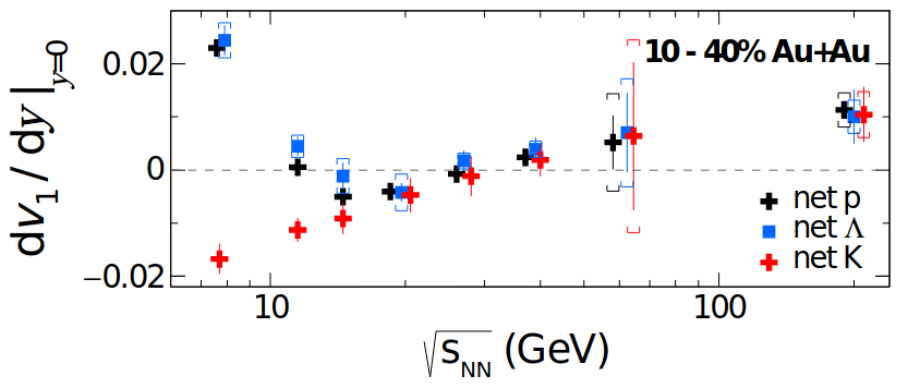
Figure 20: From Ref. Adamczyk et al. (2018b). Directed flow of net-$p$, $\Lambda$ and $K$ particle distributions at mid-rapidity as a function of the energy, for Au+Au collisions at intermediate centrality (10-40%).

VI.3.3 Elliptic flow, $v_{2}$

Elliptic flow, another name for the second flow harmonic $v_{2}$, characterises the ellipticity of the final-state particle momentum distribution, and is proportional to the initial spatial eccentricity of the collision system Snellings (2011). A nonzero value of $v_{2}$ is naturally expected to arise due to the initial asymmetry of the colliding part of the system in non-central heavy-ion collisions, especially when going towards more peripheral events, where the almond shape of the overlapping region is accentuated. The pressure gradient, created by the very high initial energy density in the overlapping region, will hence convert the spatial anisotropies into momentum anisotropies while the system cools down Snellings (2011). Using hydrodynamics or transport models, one can then extract the EoS Pratt et al. (2015) and transport coefficients of the quark-gluon plasma like the shear viscosity over entropy ratio $\eta/s$ Bernhard et al. (2019), which are nevertheless highly model-dependent and thus out of the scope of this paper. Because the connection to the EoS is highly dependent on a number of other quantities such as the initial state amongst many others, we refer an interested reader to reviews, e.g. Heinz and Snellings (2013).

Elliptic flow has been measured by several collaborations at the LHC in Pb+Pb collisions at $\sqrt{s_{NN}}=2.76$ TeV and $\sqrt{s_{NN}}=5.02$ TeV for charged particles Aad et al. (2012a); Chatrchyan et al. (2013); Acharya et al. (2018b); Chatrchyan et al. (2014a) and also for identified hadrons Abelev et al. (2015); Acharya et al. (2018c), as well as in Xe+Xe collisions at $\sqrt{s_{NN}}=5.44$ TeV Acharya et al. (2018d); Aad et al. (2020); Sirunyan et al. (2019a). At collision energies of the BESI program, between $\sqrt{s_{NN}}=7.7$ and 200 GeV, $v_{2}$ has also been extensively studied in Au+Au collision systems for both charged particles Adler et al. (2002); Back et al. (2005b, c); Adamczyk et al. (2012); Adare et al. (2015a) and identified particles Adler et al. (2001a); Adams et al. (2005c); Adamczyk et al. (2016a); Abdallah et al. (2023c) by the STAR, PHENIX and PHOBOS collaborations. Elliptic flow of smaller systems, namely Cu+Cu collisions at $\sqrt{s_{NN}}=62.4$ and 200 GeV Alver et al. (2007); Abelev et al. (2010b); Adare et al. (2015a), Ru+Ru and Zr+Zr collisions at $\sqrt{s_{NN}}=200$ GeV Sinha (2022) have been measured as well. In addition, $v_{2}$ data have also been extracted for the large, deformed system of U+U collisions at $\sqrt{s_{NN}}=193$ GeV Abdallah et al. (2021c). All of these results show two strong indicators of the common origin of produced particles from a moving fluid, namely the QGP. The first one is the mass ordering of the $p_{T}$-differential $v_{2}$ from identified hadrons at low $p_{T}$ ($<2$ GeV), with lighter species exhibiting a larger $v_{2}$ than heavier ones Abelev et al. (2010b); Adamczyk et al. (2013a). It can be understood by assuming that all particles originate from common cells of fluid with a given velocity, thus causing a shift of the $v_{2}$ signal in momentum due to the mass differences Huovinen et al. (2001); Huovinen and Ruuskanen (2006). The second one is the so-called Number of Constituent Quarks (NCQ) scaling Molnar and Voloshin (2003) at intermediate $p_{T}$ ($>1$ GeV), namely the fact that all $v_{2}$ signals from different species match when plotted as a function of $p_{T}$ or the reduced transverse mass, also called the transverse kinetic energy, $K\,E_{T}=m_{T}-m_{0}$, all of them divided by the number of valence quarks $N_{q}$ ($=2$ for mesons and $=3$ for baryons) Adare et al. (2007); Abelev et al. (2010b); Adamczyk et al. (2013a); Abelev et al. (2015); Acharya et al. (2018c, 2021d). Assuming a common origin of the produced hadrons, this scaling shown in Fig. 21 illustrates that collectivity arises from quarks as degrees of freedom, before being translated into flow of the hadrons formed by quark coalescence Fries et al. (2003); Molnar and Voloshin (2003). Such observations constitute, among other probes, a good indicator of the formation of a quark-gluon plasma. However, $N_{q}$ scaling starts breaking down in minimum bias Au+Au collisions from $\sqrt{s_{NN}}=11.5$ GeV and below, as can be seen in Fig. 21 with the $v_{2}/N_{q}$ of $\phi$ mesons (although this interpretation is discussed in Hirano et al. (2008)).

At even lower beam energies of Au+Au collisions at $\sqrt{s_{NN}}=3$ GeV, the $v_{2}$ measurements by the STAR experiment Abdallah et al. (2022a) show no $N_{q}$ scaling at all. This result tends to indicate the absence of efficient quark coalescence in the system created in such collisions, thus suggesting a dominance of the hadronic phase over deconfined partonic flow. Current hydrodynamic calculations can provide a reasonable match to experimental data down to $\sqrt{s_{NN}}=7.7$ GeV Shen and Schenke (2022) and $\sqrt{s_{NN}}=4.3$ GeV Schäfer et al. (2022). However, we point out that other effects may destroy $N_{q}$ scaling that have not yet been explored at these energies in full (3+1)D relativistic viscous hydrodynamical simulations. For example, the existence of a critical point leads to critical fluctuations that may have dramatic effects on transport coefficients, which in turn affect collective flow (see Lovato et al. (2022) for further discussion on flow at these beam energies). We also caution that NCQ scaling is only approximate and expected to hold only at intermediate $p_{T}$ Molnar and Voloshin (2003). Precise NCQ scaling for $v_{2}\{2\}(p_{T}/N_{q})/N_{q}$ is not observed even at LHC energies Abelev et al. (2015); Acharya et al. (2018c, 2021d), so one must be careful when drawing conclusions from its absence. Overall, a much clearer scaling can be seen when plotting against $K\,E_{T}/N_{q}$ Adare et al. (2007); Abelev et al. (2015).

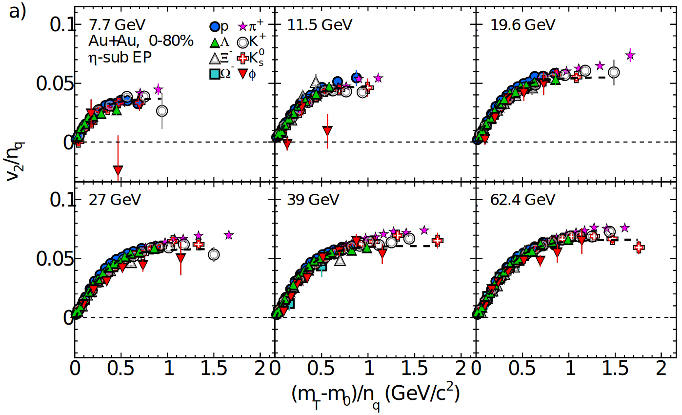
Figure 21: From Ref. Adamczyk et al. (2013a). NCQ scaling of the elliptic flow of identified hadrons ($\pi^{+}$, $K^{+}$, $K^{0}_{s}$, $\phi$, $p$, $\Lambda$, $\Xi^{-}$ and $\Omega^{-}$) for 0-80% Au+Au collisions at $\sqrt{s_{NN}}=7.7$, 11.5, 19.6, 27, 39 and 62.4 GeV.

VI.3.4 Triangular flow $v_{3}$ and beyond

Let us first discuss triangular flow before moving onto higher-order flow harmonics. The existence of triangular flow was not understood in the field of heavy-ion collisions for many years. In part, this occurred because experimentalists measured triangular flow with the wrong event plane angle (e.g. using $\Psi_{2}$ instead of $\Psi_{3}$, leading to a result of $v_{3}(\Psi_{2})=0$). However, the key issue was that the importance of event-by-event fluctuations and how significantly they could affect flow harmonics was not understood. The calculations from Takahashi et al. (2009) of 2 particle correlations, were performed in the first theoretical framework to use event-by-event fluctuating initial conditions and was the only model able to reproduce the experimental results at the time. This made it possible for experimentalists to understand the significance of triangular flow and discover the correct method for calculating it Alver and Roland (2010). This discovery of nonzero $v_{3}$ that can only arise from event-by-event fluctuating initial conditions led to a radical change in the field of heavy-ion collisions because many assumptions had to be changed, but it allowed for new ways to probe the QGP that did not exist previous to the discovery.

Higher-order flow harmonics, from $v_{3}$ and up to $v_{6}$, have also been measured in order to get complementary information concerning what can be already determined from $v_{1,2}$ results. As they require a rather high number of events to be measured with reasonable uncertainties, they have been measured almost exclusively at top energy of the BES program in Au+Au collisions, i.e. $\sqrt{s_{NN}}=200$ GeV Adare et al. (2016c); Adam et al. (2020d); Abdallah et al. (2022b), and also in Pb+Pb collisions at $\sqrt{s_{NN}}=2.76$ TeV Aamodt et al. (2011b); Aad et al. (2012a); Adam et al. (2016c); Chatrchyan et al. (2014a, b) and $\sqrt{s_{NN}}=5.02$ TeV Adam et al. (2016d); Aaboud et al. (2018); Acharya et al. (2020c), as well as in Xe+Xe collisions at $\sqrt{s_{NN}}=5.44$ TeV Acharya et al. (2018d); Aad et al. (2020). STAR (AuAu $\sqrt{s_{NN}}=7.7-200$ GeV) has now measured the suppression of $v_{3}\left\{2\right\}$ at low beam energies Adamczyk et al. (2016b) where a minimum is reached (but $v_{3}\left\{2\right\}$ does not precisely reach 0) whose results are still open for interpretation, see Fig. 22. Additionally, HADES has also calculated higher-order flow harmonics at $\sqrt{s_{NN}}=2.4$ GeV Adamczewski-Musch et al. (2020b), albeit with the event-plane method with respect to the $\Psi_{1}$ event plane angle, see Fig. 23.

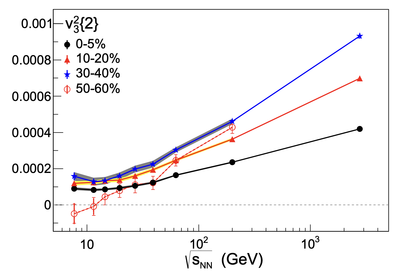
Figure 22: All charged particles $v_{3}^{2}\left\{2\right\}$ from the STAR collaboration for various centralities in Au+Au collisions at $\sqrt{s_{NN}}=7.7$, 11.5, 19.6, 27, 39 and 62.4 GeV. Taken from Adamczyk et al. (2016b).

Figure 23: All charged particles collective flow from HADES in Au+Au collisions at $\sqrt{s_{NN}}=2.4$ GeV. Taken from Adamczewski-Musch et al. (2020b).

In the context of BESI, the STAR collaboration has performed a comprehensive analysis of 3-particle azimuthal anisotropy correlations $C_{m,n,m+n}$, between different harmonics $m$, $n$ and $m+n$, over a wide range of multiplicities, transverse momenta, and energies from $\sqrt{s_{NN}}=7.7$ GeV to $200$ GeV Adamczyk et al. (2018d). The dependence displayed by results on the pseudo-rapidity differences between particles suggests the breaking of longitudinal boost invariance or dominance of unconventional non-flow contributions.

VI.3.5 4+ particle flow cumulant observables

The multi-particle cumulant method used to extract $v_{n}\{2\}$ in Eq. (30) can be extended to cumulants of higher order, denoted $v_{n}\{2k\}$ Borghini et al. (2001b, a, c); Bilandzic et al. (2011, 2014); Di Francesco et al. (2017); Moravcova et al. (2021). In general, measurements of $v_{n}\{2k\}$ depend on irreducible $2k$-particle correlations, so that non-collective contributions to $v_{n}$ are suppressed by a combinatorial factor, which decreases with $k$. The four-particle $v_{n}\{4\}$, for instance, is given by

$$-v_{n}\{4\}^{4}=\langle v_{n}^{4}\rangle-2\,\langle v_{n}^{2}\rangle^{2}\ ,$$ (34)

where $2$-particle contributions are subtracted by the second term (see, for instance Giacalone et al. (2017)).

Non-flow contributions set aside, differences between multi-particle cumulants are also sensitive to how the coefficients $v_{n}$ fluctuate event-by-event Aad et al. (2013, 2014a). In the regime in which these coefficients scale linearly with anisotropies of the initial state, i.e. $v_{n}\propto\varepsilon_{n}$ Teaney and Yan (2011); Gardim et al. (2012); Niemi et al. (2013); Teaney and Yan (2012); Qiu and Heinz (2011); Gardim et al. (2015); Betz et al. (2017), where $\varepsilon_{n}$ quantifies the initial-state anisotropy, ratios between different cumulants depend only on fluctuations of the initial anisotropies, characterized by cumulants $\varepsilon_{n}\{2k\}$ Ma et al. (2016); Giacalone et al. (2017). For instance,

$$\frac{v_{n}\{2k\}}{v_{n}\{2\}}\approx\frac{\varepsilon_{n}\{2k\}}{\varepsilon_{n}\{2\}}\ ,$$ (35)

where the proportionality factor relating initial-state and flow anisotropy cancels out Yan and Ollitrault (2014), so that multi-particle flow measurements can be employed to isolate information on initial-state fluctuations from information on the response of the medium Giacalone et al. (2017); Bhalerao et al. (2019a, b). However, in peripheral collisions Noronha-Hostler et al. (2016b), small systems Sievert and Noronha-Hostler (2019), differential flow Hippert et al. (2020a), and to a much lesser extent lower beam energies Rao et al. (2021) this linear scaling begins to break down, and it requires non-linear response as well. Multiparticle cumulants and fluctuations of flow coefficients have been measured at $\sqrt{s_{NN}}=130$ GeV by the STAR collaboration Adler et al. (2002), across BESI $\sqrt{s_{NN}}=7.7-200$ GeV from the STAR collaboration Abdallah et al. (2022c), and at $\sqrt{s_{NN}}=2.76-5.02$ TeV by ATLAS, CMS and ALICE in Pb+Pb collisions Aad et al. (2013, 2014a); Sirunyan et al. (2019b, 2018a); Acharya et al. (2018b), by ALICE, CMS, and ATLAS in p-Pb collisions Abelev et al. (2014c); Khachatryan et al. (2015a, 2017); Sirunyan et al. (2018a); Aaboud et al. (2017a); Acharya et al. (2019b), and by ALICE in p+p and Xe+Xe collisions Acharya et al. (2019b).

While multi-particle cumulants of a single flow coefficient can be used as proxies of its fluctuations, correlations between different coefficients can be studied with so-called symmetric cumulants Bilandzic et al. (2014)

$$\textrm{SC}(n,m)=\langle v_{n}^{2}\,v_{m}^{2}\rangle-\langle v_{n}^{2}\rangle\langle v_{m}^{2}\rangle\ ,$$ (36)

or normalized symmetric cumulants $\textrm{sc}(m,n)=\textrm{SC}(n,m)/(\langle v_{n}^{2}\rangle\langle v_{m}^{2}\rangle)$ Bhalerao et al. (2011, 2019a); Moravcova et al. (2021), which can also be generalized to higher orders Mordasini et al. (2020). For symmetric cumulants, it is important to ensure that multiplicity weighing and centrality binning are taken into account in order to reproduce experimental data Gardim et al. (2017).

Normalized symmetric cumulants are related to event-plane correlations Bhalerao et al. (2015a); Giacalone et al. (2016), which can be quantified by examining how combinations of event planes for different harmonics, $\Psi_{n_{1},n_{2},\ldots,n_{k}}\equiv a_{1}\Psi_{n_{1}}+a_{2}\Psi_{n_{2}}+\ldots+a_{m}\Psi_{n_{k}}$ fluctuate Jia and Mohapatra (2013); Jia and Teaney (2013); Bhalerao et al. (2011); Qin and Muller (2012). Taking the Fourier series of the distribution $dN/d\Psi_{n_{1},n_{2},\ldots,n_{k}}$, one finds coefficients

$$V^{j}_{n_{1},n_{2},\ldots,n_{k}}\equiv\langle\cos\left(j\,\Psi_{n_{1},n_{2},\ldots,n_{k}}\right)\rangle\ ,$$ (37)

where $n$-fold symmetry of the event-plane angle $\Psi_{n}$ requires that $a_{i}=n_{i}\,c_{i}$, $c_{i}\in\mathcal{Z}$, and invariance of correlations under global rotations imposes that $\sum_{i}n_{i}\,c_{i}=0$. The event-plane correlations have been suggested as a method to possibly constrain viscous effects Niemi et al. (2016).

The PHENIX collaboration has investigated event-plane correlations in Au+Au collisions at $\sqrt{s_{NN}}=200$ GeV at RHIC Adare et al. (2011). Results for symmetric cumulants and normalized symmetric cumulants in Au+Au collisions at center-of-mass energies of $\sqrt{s_{NN}}=27$ GeV, $39$ GeV, $54.4$ GeV and $200$ GeV were also published by STAR in Adam et al. (2018); STA (2023), where they are compared to LHC results. ATLAS and ALICE have performed measurements of event-plane correlations in Pb+Pb collisions at $\sqrt{s_{NN}}=2.76$ TeV Aad et al. (2014b); Acharya et al. (2017a), while ALICE, CMS, and ATLAS have published measurements of symmetric cumulants Adam et al. (2016e); Sirunyan et al. (2018b); Aaboud et al. (2019); Acharya et al. (2021e).

VI.3.6 Differential flow and scalar products

Another important tool for constraining QGP properties is the study of flow anisotropies differentially in transverse momentum $p_{T}$ or (pseudo-rapidity $\eta$) Luzum and Romatschke (2008); Schenke et al. (2012); Nijs et al. (2021). In theory this amounts to considering the $p_{T}$ in Eq. (20), so that the flow coefficients become $v_{n}=v_{n}(p_{T})$. In practice, this entails binning particles of interest according to their momenta. However, a good determination of the reference event plane $\psi_{n}$ demands that particles of reference be defined over a wider and suitably chosen momentum range. The differential flow coefficients can thus be found from the scalar product of Eq. (32) (see e.g. Bilandzic et al. (2011) for details).

Flow harmonics in different $p_{T}$ regions reveal different physics. In the low $p_{T}$ region, differential flow observables allow for the investigation of the hydrodynamic response of the QGP as a function of transverse momentum. As discussed above, the mass ordering of elliptic flow at low $p_{T}$, with lighter particles presenting stronger flow, has been regarded as a signature of hydrodynamic expansion, while the NCQ scaling of flow harmonics at intermediate $p_{T}$ has been viewed as a signature of quark coalescence Huovinen et al. (2001); Molnar and Voloshin (2003); Gyulassy (2004); Gyulassy and McLerran (2005); Huovinen and Ruuskanen (2006); Adams et al. (2005c); Abelev et al. (2008b, b). At higher $p_{T}$, flow harmonics encode information on energy loss Gyulassy et al. (2001); Wang (2001).

Differential flow harmonics have been measured for a variety of systems and beam energies. For Pb+Pb collisions, at the LHC differential flow measurements have been made at $\sqrt{s_{NN}}=2.76$ TeV from ALICE Aamodt et al. (2011b), CMS Chatrchyan et al. (2012) and ATLAS Aad et al. (2012b), and at $\sqrt{s_{NN}}=5.02$ GeV from ALICE Adam et al. (2016d); Acharya et al. (2018c); ALI (2022d) and CMS Sirunyan et al. (2018c, 2020). Measurements have also been performed at RHIC at high beam energies for Au+Au Adams et al. (2005d); Adler et al. (2003); Afanasiev et al. (2009); Adler et al. (2004); Back et al. (2005c), Cu+Cu Adare et al. (2015a) and Cu+Au Adare et al. (2016b) collisions at $\sqrt{s_{NN}}=200$ GeV and $62.4$ GeV Adare et al. (2015a), and Au+Au collisions at $\sqrt{s_{NN}}=130$ GeV Ackermann et al. (2001). A comprehensive analysis of p+Au, d+Au, Cu+Cu and Cu+Au collisions at $\sqrt{s_{NN}}=200$ GeV, as well as U+U collisions at $\sqrt{s_{NN}}=193$ GeV, from the STAR collaboration can be found in Adam et al. (2019c). In the context of the BESI there have been measurements from $\sqrt{s_{NN}}=7.7-200$ GeV Adamczyk et al. (2013b, 2016a); Abelev et al. (2008b).

At very low beam energies, sometimes differential flow measurements are reported in terms of the transverse mass $m_{T}$ such that this is related to $p_{T}$ through

$$m_{T}=\sqrt{m^{2}+p_{T}^{2}}\ ,$$ (38)

where $m$ is the mass of the particle(s) considered. If only one particle species is considered in the flow, it is possible to translate between $p_{T}$-dependent flow and $m_{T}$-dependent flow. However, if multiple identified particles are considered, it is not possible to make this translation without more information from the experiment. Fixed target measurements have been made at the STAR fixed target program for $\sqrt{s_{NN}}=3$ GeV Abdallah et al. (2022a) (in this work it was also normalized by the number of quarks such that $N_{q}=2$ for mesons and $N_{q}=3$ for baryons) for $\sqrt{s_{NN}}=4.5$ GeV Adam et al. (2021b). At HADES, using Au-Au collisions at $\sqrt{s_{NN}}=2.4$ GeV Adamczewski-Musch et al. (2020b), differential flow was measured in terms of $m_{T}$. Differential flow provides a more stringent test for models of strongly interacting matter, with transport models, represented by SMASH Mohs et al. (2022), currently unable to reproduce results from HADES Kardan (2019) (although this may be fixed with further improvements Sorensen et al. (2023)).

An interesting consequence of the $p_{T}$ dependence of flow coefficients is that one may investigate how anisotropies over different $p_{T}$ ranges correlate with one another Kikola et al. (2012); Gardim et al. (2013); Heinz et al. (2013). In particular, 2-particle correlations are given by the covariance matrix

$$V_{n\Delta}^{ab}\equiv V_{n\Delta}(p_{T}^{a},p_{T}^{b})=\langle V_{n}^{*}(p_{T}^{a})\,V_{n}(p_{T}^{b})\rangle\ ,$$ (39)

where $p_{T}^{(a,b)}$ denote the transverse momentum in two $p_{T}$ bins $a$ and $b$, and we generalize the complex $V_{n}=v_{n}\,e^{i\Psi_{n}}$ of Eq. (21) for differential flow. In the absence of flow fluctuations or non-flow effects, independent particle emission from the fluid implies that the covariance matrix “factorizes” as $V_{n\Delta}^{ab}=v_{n}(p_{T}^{a})\,v_{n}(p_{T}^{b})$. The breaking of this factorization can signal non-flow contributions Kikola et al. (2012); Jia (2011); Adare (2011); Aad et al. (2012a) or, more interestingly, event-by-event flow fluctuations Gardim et al. (2013), and can be quantified by the factorization-breaking coefficient

$$r_{n}(p_{T}^{a},p_{T}^{b})\equiv\frac{V_{n\Delta}(p_{T}^{a},p_{T}^{b})}{\sqrt{V_{n\Delta}(p_{T}^{a},p_{T}^{a})\,V_{n\Delta}(p_{T}^{b},p_{T}^{b})}}\leq 1\ ,$$ (40)

with the inequality being saturated for the case of perfect factorization. The same coefficient can be defined for pseudo-rapidity instead of transverse-momentum bins. Equation (40) is such that, in the regime of linear response to initial anisotropies, the response of the medium cancels out and $r_{n}$ is determined mainly by initial-state fluctuations. This coefficient, and its counterpart for $\eta$-differential flow, has been measured by CMS for both Pb+Pb collisions at $\sqrt{s_{NN}}=2.76$ TeV and p-Pb collisions at $\sqrt{s_{NN}}=5.02$ TeV Khachatryan et al. (2015b); Sirunyan et al. (2017), and was found to be generally close to, yet below 1.

Factorization breaking can also be understood in terms of the spectral decomposition and principal component analysis of $V_{n\Delta}^{ab}$, with the case of perfect factorization corresponding to a single nonzero eigenvalue. The principal component analysis of flow fluctuations was proposed in Bhalerao et al. (2015b) as a more transparent alternative to $r_{n}$, and measured by CMS, in Pb+Pb collisions, at $\sqrt{s_{NN}}=2.76$ TeV Sirunyan et al. (2017). However, it has been suggested that the original prescription for carrying out this measurement led to the contamination of subleading anisotropic flow modes by fluctuations of radial flow Hippert et al. (2020b). Results from hydrodynamic simulations indicate that the factorization-breaking coefficient and subleading components of the PCA of $V_{n\Delta}$ are capable of probing initial-state fluctuations at smaller length-scales, compared to the initial transverse size of the system Kozlov et al. (2014); Gardim et al. (2018); Hippert et al. (2020a).

VI.4 HBT

Hanbury Brown–Twiss (HBT) interferometry Heinz and Jacak (1999); Wiedemann and Heinz (1999); Lisa et al. (2005) provides a way to probe the space-time evolution of heavy-ion collisions using correlations between pairs of identical particles emitted from these collisions, such as pions or kaons. By analyzing the resulting two-particle correlation functions at small relative momentum, one finds that their inverse widths (the ‘HBT radii’ $R^{2}_{ij}$) correspond to the average separation between the emission points of any two identical particles, and, therefore, provide a way of quantifying the space-time structure of the particle emission process. Insofar as the bulk of particle production occurs towards the end of the system’s lifetime Plumberg and Heinz (2015); Müller and Schäfer (2022), one expects that HBT measurements should be sensitive to the entire history of the fireball, and, therefore, should depend on the EoS as well.

This expectation turns out to be correct. Previous studies have established at least five different connections between HBT and the nuclear EoS. First, the space-time information extracted from HBT can be used to estimate the volume of the system at freeze out. The freeze-out volume can then be used to estimate the peak energy density and, thereby, obtain evidence for the onset of deconfinement Heinz and Jacak (1999); Lisa et al. (2005). Second, the specific observables $R^{2}_{o}-R^{2}_{s}$ and $R_{o}/R_{s}$ are sensitive to the emission duration and rate of expansion of the collision system Heinz and Jacak (1999); Pratt (2009); Adamczewski-Musch et al. (2019b); measuring these quantities as functions of the pair momentum $K_{T}$ can constrain the existence or absence of a first-order phase transition at different beam energies and chemical potentials Lisa et al. (2005); Li et al. (2023). For the same reason, these observables have also been identified as potential signatures of the QCD critical point, by analyzing their scaling with beam energy $\sqrt{s_{NN}}$ to signal a softening in the EoS Lacey (2015). A third connection between HBT and the nuclear equation state uses the moments of collision-by-collision fluctuations in the HBT radii to isolate the geometric effects of critical fluctuations on the system’s evolution Plumberg and Kapusta (2017), and thereby provides an independent way of probing the QCD critical point. Fourth, HBT is sensitive to the speed of sound as a function of temperature. HBT measurements in different collision systems and beam energies (Au+Au at RHIC vs. Pb+Pb at the LHC) have been shown in a multi-observable Bayesian analysis Pratt et al. (2015); Sangaline and Pratt (2016) to directly constrain a parameterized form of $c_{s}^{2}(T)$. Fifth, the multiplicity dependence of the HBT radii in different size collision systems – specifically, the slope of $R_{ij}$ vs. $(dN_{ch}/d\eta)^{1/3}$ in p+p, p+Pb, and Pb+Pb – may also reflect the influence of $c^{2}_{s}$ on the rate of the system’s expansion Plumberg (2020).

In addition to these examples, the global shape of the fireball at freezeout is sensitive to the EoS in at least two ways. First, the HBT radii can be analyzed experimentally as functions of the azimuthal pair emission angle $\Phi_{K}$, which indicates the direction of a given particle pair’s average momentum in the transverse plane. By expanding this azimuthal dependence in a Fourier series and studying the extracted coefficients as functions of $\sqrt{s_{NN}}$, one acquires sensitivity to the EoS via the freeze-out eccentricity $\varepsilon_{F}$ (roughly, the normalized second-order Fourier coefficients of the $R^{2}_{ij}$), which measures the extent to which the initial elliptic geometry of the collision system is inverted by the subsequent dynamical expansion Adamczyk et al. (2015); Adamczewski-Musch et al. (2020c). Second, one can also observe sensitivity to the EoS in the transition from prolate to oblate freezeout configurations, which is done by correlating transverse and longitudinal HBT radii as a function of collision energy. The resulting non-monotonic trend observed in the data Adam et al. (2021b) is attributed to a transition from dynamical evolution dominated by nucleon stopping at low energies to boost-invariant evolution at higher energies.

HBT measurements have been carried out in a vast number of different collision systems and over a wide range of collision energies and particle species. We focus here on HBT with Bose-Einstein correlations, primarily using charged pion pairs. Important recent measurements include: azimuthally sensitive analyses in Pb+Pb at 2.76 TeV Adamova et al. (2017); Acharya et al. (2018e), p+Pb at 5.02 TeV ATL (2017), Cu+Au and Au+Au Lisa et al. (2000); Adams et al. (2004, 2005e); Adare et al. (2014); Khyzhniak (2020a), and Pb+Au at 40, 80, and 158 GeV Adamová et al. (2003); Adamova et al. (2008). The majority of studies present results for azimuthally averaged analyses. At the LHC, HBT has been measured: by ALICE, in Pb+Pb at 2.76 TeV Aamodt et al. (2011c), p+p at 0.9 and 7 TeV Aamodt et al. (2011d); Acharya et al. (2019c); by CMS, in p+p, p+Pb, and Pb+Pb at various energies 0.9, 2.76, 5.02, and 7 TeV; and by ATLAS in p+Pb at 5.02 TeV Aaboud et al. (2017b). At RHIC, STAR has further measured HBT: in U+U collisions at 193 GeV Campbell (2018); in Au+Au at collision energies of $\sqrt{s_{NN}}=4.5$, 7.7, 9.2, 11.5, 19.6, 27, 39, 62.4, 130, and 200 GeV Adler et al. (2001b); Abelev et al. (2010a); Anson (2011); Adamczyk et al. (2015); Zbroszczyk (2022); in p+Au and d+Au at 200 GeV Khyzhniak (2020b); and in p+p collisions at 200 GeV Aggarwal et al. (2011). PHENIX has conducted measurements in d+Au and Au+Au at 200 GeV Ajitanand et al. (2014) and in Au+Au at 7.9, 19.6, 27, 39, 62, and 200 GeV Soltz (2014). Au+Au collisions have been further studied by the HADES collaboration at 2.4 GeV Adamczewski-Musch et al. (2019b, 2020c); Greifenhagen (2020). The majority of analyses study two-pion correlations for statistical reasons, but HBT has also been studied for kaon pairs by various collaborations at both RHIC and the LHC Adamczyk et al. (2013c); Nigmatkulov (2016); Acharya et al. (2017b, 2019d) and for multi-pion correlations in various systems Adare et al. (2015b); Adam et al. (2016f).

VII Experimental Constraints: Low-energy Nuclear Physics

In the following section, we will review various empirical observations of constraints relevant to low-energy nuclear physics for isospin-symmetric and asymmetric matter.

VII.1 Isospin symmetric matter at saturation density

As neutron stars are in many ways like giant nuclei with $\sim 10^{57}$ nucleons Glendenning (1997), at densities which are typical of nuclei they should reproduce the same properties. Therefore, astrophysicists use laboratory measurements of nuclear experiments to calibrate neutron stars (or dense matter in general) properties. Low-energy laboratory conditions can be considered at $T\sim 0$ when describing fermions, as their order of chemical potential and mass are 10⁵ times larger than the temperature of fully evolved neutron stars (10^-2 MeV $\sim 10^{8}$ K) and even more when compared to laboratories. At effectively zero temperature, antifermions do not contribute and the relevant degrees of freedom at $n_{sat}$ are nuclei (composed of neutrons and protons), which are approximately isospin symmetric, with charge fraction $Y_{Q}\sim 0.5$. The minimal condition on any dense matter theory is to reproduce the experimental results of zero temperature, isospin symmetric nuclear matter at saturation: saturation density $n_{sat}$, binding energy per nucleon $B/A$, and compressibility $K$. Additionally, for models that contain exotic degrees of freedom, hyperon potentials $U_{H}$ and $\Delta$-baryon potential $U_{\Delta}$ can be used.

These empirical values are known within uncertainties and are extracted using extrapolation within phenomenological models, since infinite nuclear matter does not exist. Here, we enlist various empirical investigations of the above-mentioned properties. The values for the observables related to isospin-symmetric nuclear matter are summarized in Table 5, those related to exotic matter in Table 6.

VII.1.1 Saturation density

The saturation density (actually the number density, as it defines the number of baryons per volume) indicates that there is a size saturation in atomic nuclei, preventing them from contracting or collapsing as a result of the nuclear force’s powerful attraction and repulsion. This is the most important constraint, as often other constraints are determined at this density.

The simplest way to calculate a given number density is by dividing the number of baryons in a nucleus over the volume of the nucleus, as Haensel et al. (1981)

$$n_{sat}=\frac{A}{4\pi R^{3}/3}=\frac{3}{4\pi(R/A^{1/3})^{3}}=\frac{3}{4\pi R_{0}^{3}}=0.17\pm 0.03~{}~{}\mathrm{fm}^{-3}\ ,$$ (41)

where it was assumed that the value of the nuclear radius constant is $R_{0}=R/A=1.04-1.17$ fm. The error-bar reflects the uncertainty on $R_{0}$, obtained in several non-relativistic semi-empirical approaches Myers and Swiatecki (1966); Myers (1977); Barrett (1974). More modern relativistic approaches use the relation between baryon density and Fermi momentum Gross-Boelting et al. (1999); Blaizot (1980)

$$n_{sat}=\frac{2k_{F}^{3}}{3\pi^{2}}\sim 0.148-0.185~{}~{}\mathrm{fm}^{-3}\ ,$$ (42)

with $k_{F}$=1.3-1.4 fm^-1 (see Fig. 24) calculated using the Coester line, a relation between Fermi momentum and the inferred binding energy per nucleon Gross-Boelting et al. (1999)).

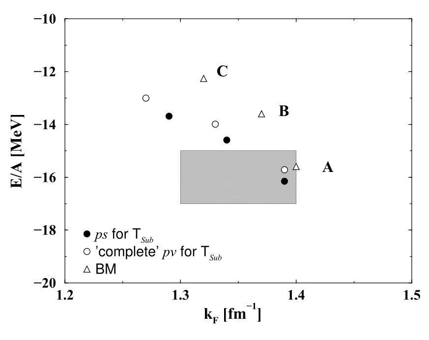
Figure 24: From Ref. Gross-Boelting et al. (1999). Binding energy per nucleon vs. Fermi momentum, with the shaded box representing saturation. The Bonn potentials shown via letters A, B, and C are used for bare nucleon-nucleon interaction. In addition, the three legends describe the T-matrix calculations using a subtraction scheme with the $ps$ representation (top), the $pv$ representation (middle), and Brockmann and Machleidt, $BM$ (bottom) Brockmann and Machleidt (1990).

Recently, in the elastic scattering of longitudinally polarized electrons extracted from ²⁰⁸Pb, the PREX collaboration reported a precise measurement of the parity-violating asymmetry A_PV term Adhikari et al. (2021), where the interior baryonic density at saturation was derived from the measured interior weak density $n^{0}_{W}$ i.e.

$$n_{sat}=0.1480\pm 0.0038~{}~{}\mathrm{fm}^{-3}\ .$$ (43)

Here, the uncertainty contains both theoretical and experimental contributions.

VII.1.2 Binding energy per nucleon at saturation

Binding energy ($B$) is the energy required to separate a nucleus, and is given by the semi-empirical mass formula

$$B=a_{v}A-a_{s}A^{2/3}-a_{c}\frac{Z(Z-1)}{A^{1/3}}-a_{a}\frac{(N-Z)^{2}}{A}+a_{p}\frac{1}{A^{1/2}}\ ,$$ (44)

with the first term representing the volume effects ($B_{\mathrm{vol}}$), the second term denoting the surface effects ($B_{\mathrm{surf}}$), the third term describing the Coulomb interactions ($B_{\mathrm{Coul}}$), the fourth term describing the effect of isospin asymmetry ($B_{\mathrm{asym}}$), and the last term covering the effects of the pairing ($B_{\mathrm{p}}$). Since there are no surface effects and Coulomb effects are also ignored in infinite isospin-symmetric nuclear matter, the net binding energy is approximated as the binding energy’s volume term ($B\approx B_{vol}$). In Ref. Myers and Swiatecki (1966), the volume term of the binding energy per nucleon $B/A$=-15.677 MeV at $n_{sat}$=0.16146 fm^-3 was obtained from a non-relativistic semi-empirical four-parameter mass formula with coefficients from the liquid-drop model using the experimental masses of 49 heavy nuclei. In addition, using experimental data from 1654 ground state masses of nuclei with N, Z $\geq$ 8, $B/A$=-16.24 MeV at $n_{sat}$=0.16114 fm^-3 was obtained from non-relativistic semi-empirical four-parameter mass formula with coefficients from shell-corrected Thomas-Fermi model Myers and Swiatecki (1996).

VII.1.3 Compressibility at saturation

The incompressibility, usually referred to as compressibility, or compression modulus $K_{\infty}=9\frac{dP}{dn_{B}}$ of infinite nuclear matter is considered one of the vital constraints for dense matter, as it determines the stiffness of the EoS. In finite nuclear systems, the isoscalar giant monopole resonance (ISGMR) establishes a direct empirical link between the finite nucleus compressibility, $K_{A}$ and the centroid energy $E_{\mathrm{ISGMR}}$ Colo et al. (2014),

$$E_{\mathrm{ISGMR}}=\sqrt{\frac{\hbar^{2}K_{A}}{m\left\langle r^{2}\right\rangle_{m}}}\ ,$$ (45)

where $\left\langle r^{2}\right\rangle_{m}$ is the mean square mass-radius in the ground state and $m$ is the nucleon mass.

Furthermore, the finite compressibility can be expressed in terms of the liquid-drop mass formula Blaizot (1980)

$$K_{A}=K_{\mathrm{vol}}+K_{\mathrm{surf}}A^{-1/3}+K_{\mathrm{asym}}\Big{(}\frac{N-Z}{A}\Big{)}^{2}+K_{\mathrm{Coul}}\frac{Z^{2}}{A^{4/3}}\ ,$$ (46)

where $K_{\mathrm{vol}}$, $K_{\mathrm{surf}}$, $K_{\mathrm{asym}}$ and $K_{\mathrm{Coul}}$ define the volume, surface, asymmetry and Coulomb terms, respectively. The $K_{\mathrm{vol}}$ term is related to the nuclear matter properties such that $K_{\mathrm{vol}}\approx K_{\infty}$ Blaizot (1980). Inelastic scattering of isoscalar probes can be used to determine the ISGMR strength distribution experimentally. The $\alpha$ particle has been the most widely used and emerges as effective probe for such observations. The discussion of ISGMR collective nucleon excitations from ⁹⁰Zr and ²⁰⁸Pb nuclei suggests $K_{\infty}=240\pm 20$ MeV Colo et al. (2014); Todd-Rutel and Piekarewicz (2005); Colo et al. (2004); Agrawal et al. (2003), but there might be a softening in this value caused by pairing Cao et al. (2012); Vesely et al. (2012).

In Ref. Khan and Margueron (2012), the authors argue that properties of nuclei do not set constraints on the EoS at saturation density, but rather at an average density of $\sim 0.11$ fm^-3, that they design as crossing density. Considering that the giant monopole resonance of a chain of nuclei constrains the third derivative of the energy per unit of volume at this density, they arrive at $K_{\infty}=230\pm 40$ MeV with 17% uncertainty.

In another work, the authors reviewed in detail the methods of analysis of giant monopole resonance (GMR) data, as well as values obtained using different techniques and theories between 1961 and 2016 covering a range $K_{\infty}=100-380$ MeV (see references within table 1 of Ref. Stone et al. (2014)), with a trend to higher values in relativistic than in non-relativistic mean-field models. Without any microscopic model assumptions, except (marginally) the Coulomb effect, $250<K_{\infty}<315$ MeV was obtained and it was shown that surface characteristics have a crucial influence in vibrating nuclei Stone et al. (2014).

Constraints	Value	Reference
Saturation density, $n_{sat}$ (fm-3)	0.17 $\pm$ 0.03	Haensel et al. (1981)
	0.148 - 0.185	Gross-Boelting et al. (1999)
	0.148 $\pm$ 0.0038	Adhikari et al. (2021)
Binding energy per nucleon, $B/A$ (MeV)	-15.677	Myers and Swiatecki (1966)
	-16.24	Myers and Swiatecki (1996)
Compressibility, $K_{\infty}$ (MeV)	240 $\pm$ 20	Colo et al. (2014); Todd-Rutel and Piekarewicz (2005); Colo et al. (2004); Agrawal et al. (2003)
	210 - 270	Khan and Margueron (2012)
	251 - 315	Stone et al. (2014)

Table 5: Experimental constraints related to isospin-symmetric nuclear matter at saturation.

VII.1.4 Hyperon potentials

In this section, we list various experimental results relevant to hyperon potentials. In relativistic models, the hyperon potential is defined as $U_{H}$=vector interaction+scalar interaction, while in non-relativistic models it is defined as $U_{H}=E_{H}-T_{H}-m_{H}$, the difference between single-particle energy and kinetic energy (plus mass), both usually discussed at saturation. Although more constraining data exists for the potential of the $\Lambda$ hyperon, data also exists for the $\Sigma$ and $\Xi$ potentials.

The analysis of data from the level spectra of $\Lambda$ hypernuclei from $\pi^{+}K^{+}$ and $K^{-}\pi^{-}$ reactions produced at emulsion and bubble chambers showed that the single-particle energies of $\Lambda$-hypernuclei vary smoothly with number of nucleons $A$ and are well reproduced considering the potential at nuclear saturation density $U(\Lambda-N)\equiv U_{\Lambda}=-28$ MeV Millener et al. (1988). Considering a slightly different renormalization of the data obtained from the KEK 12-GeV PS and superconducting kaon spectrometer (SKS) Hasegawa et al. (1996), the value $U_{\Lambda}=-30$ MeV was obtained in Ref. Gal et al. (2016). In Ref. Shen et al. (2006), using a relativistic mean-field approach, in particular the TM1 model Sugahara and Toki (1994), the data of Ref. Hasegawa et al. (1996) have been used to fit the $\sigma$-$\Lambda$ coupling, while considering that the $\Lambda$-vector mesons couplings are determined from the SU(6) quark model. A $\Lambda$-hyperon potential in nuclear matter at saturation density equal to $U_{\Lambda}=-30$ MeV was obtained. Similar values, $U_{\Lambda}=-30$ to $-32$ MeV, have been obtained with other relativistic mean-field models using the same constraints Fortin et al. (2018).

As discussed in Ref. Gal et al. (2016), measurements at KEK (the High Energy Accelerator Research Organization in Japan) of the $\Sigma^{-}$ spectrum Noumi et al. (2002); Saha et al. (2004) have indicated that the $\Sigma$-nucleon potential is strongly repulsive. A $\Sigma$ potential in symmetric nuclear matter considered reasonable is of the order $U_{\Sigma}=30\pm 20$ MeV Gal et al. (2016). Note that the $\Sigma$-hyperon is predicted by some models, such as the QMC model, not to appear in dense matter for the regime relevant for neutron stars Stone et al. (2021).

Concerning the $\Xi$-nucleon potential, the measurement of ${}^{12}_{\Xi}$Be Khaustov et al. (2000) was described with a Wood-Saxon potential of the order of $U_{\Xi}=-14$ MeV Gal et al. (2016). The more recent Kiso event Nakazawa et al. (2015) for ${}^{15}_{\Xi}$Ca, if interpreted as a 1$p$ state, seems to indicate a deeper potential. Relativistic mean field models have been constrained by this measurement and a depth of the order of $U_{\Xi}=-15$ to $-19$ MeV was obtained Fortin et al. (2020). Recently, considering five two-body $\Xi$ capture events to two single $\Lambda$-hypernuclei obtained by KEK Aoki et al. (2009); Nakazawa et al. (2015) and J-PARC (the Japan Proton Accelerator Research Complex) Hayakawa et al. (2021), the authors of Friedman and Gal (2021) have calculated an attractive $\Xi$-nucleon interaction with a depth $U_{\Xi}\gtrsim 20$ MeV ($U_{\Xi}=21.9\pm 0.7$ MeV).

Note, however, that a much less attractive $\Xi$ potential has been calculated by the HAL-QCD collaboration Inoue (2019). Using hyperon interactions extracted from a (2+1) lattice QCD in Brueckner-Hartree-Fock (BHF) calculation with a statistical error of approximately $\pm$2 MeV related with the QCD Monte Carlo simulation, the HAL QCD collaboration anticipated $U_{\Lambda}=-28$ MeV, $U_{\Sigma}=+15$ MeV, and $U_{\Xi}=-4$ MeV Inoue (2019) at $n_{sat}$, which agrees with $p-\Xi^{-}$ correlation functions from the ALICE collaboration using 3-momenta measured at $s=\sqrt{13}$ TeV Fabbietti et al. (2021); Collaboration et al. (2020).

VII.1.5 $\Delta$-baryon potential

Here, we list the empirical observations of spin 3/2 $\Delta$ baryon-nucleon potential at saturation, which is a helpful quantity when constraining its values in dense matter models. As already discussed, $\Delta$’s can replace hyperons without softening the EoS as much, which can be a solution to the hyperon puzzle Bednarek et al. (2012).

The introduction of a phenomenological $\Delta$-nucleus spin-orbit interaction was used to improve the fit to the experimental $\pi$-nucleus angular distributions for $\pi-^{16}$O at 114 and 240 MeV, $\pi-^{4}$He at 220 and 260 MeV and $\pi-^{12}$C at 180 and 200 MeV Horikawa et al. (1980). It was anticipated that the strength of the $\Delta$-nucleus spin-orbit interaction term is similar (attractive) to the nucleon-nucleon one, i.e. $U_{\Delta}\approx U_{N}$ Horikawa et al. (1980). In another study, the cross-section measurement of electron-nucleus scattering observed in 2.5 GeV Synchrotron at Bonn gives a density-dependent average binding potential $U_{\Delta}(n_{B})\simeq$ $-75$ $n_{B}(r)/n_{sat}$ MeV Koch and Ohtsuka (1985). Furthermore, a range of uncertainty is estimated from the electron-nucleus, pion nucleus, scattering and photoabsorption experiments i.e. $-30$ MeV $+U_{N}<U_{\Delta}<U_{N}$, with $U_{N}\simeq-(50-60)$ MeV, which leads to the constraint $-90$ MeV $<U_{\Delta}<-50$ MeV Drago et al. (2014).

Constraints	Value	Reference
Hyperon Potentials (MeV)	$U_{\Lambda}$ = -28	Inoue (2019); Millener et al. (1988)
	$U_{\Lambda}$ = -30	Gal et al. (2016)
	$U_{\Sigma}$ = 15	Inoue (2019)
	$U_{\Sigma}$ = 10-50	Gal et al. (2016)
	$U_{\Xi}$ = $-14$	Gal et al. (2016)
	$U_{\Xi}$ = $-21.9\pm 0.7$	Friedman and Gal (2021)
	$U_{\Xi}$ = -4	Inoue (2019)
Delta Baryon Potential (MeV)	$U_{\Delta}\sim U_{N}$	Horikawa et al. (1980)
	$U_{\Delta}(n_{B})$ = -75 $n_{B}(r)/n_{sat}$	Koch and Ohtsuka (1985)
	$-90<U_{\Delta}<-50$	Drago et al. (2014)

Table 6: Empirical constraints related to isospin-symmetric exotic matter at saturation.

VII.2 Symmetry energy $E_{sym}$ and derivative $L$

To translate between isospin symmetric matter and matter in neutron stars, with very low charge fraction, we make use of the symmetry energy $E_{sym}$. The determination of the saturation density $E_{\rm{sym}}$, $L$, $K_{sym}$, and $J$ parameters is very challenging, and involves large experimental and theoretical efforts Estee et al. (2021). At low densities, we have some fundamental understanding of the symmetry energy but, at large densities, the uncertainty becomes extremely large. At subsaturation densities, nuclear structure probes can generally confine the symmetry energy most effectively, whereas astronomical observations and heavy-ion collisions are two significant methods for constraining the symmetry energy from subsaturation to suprasaturation densities Zhang and Chen (2015). The main source of uncertainty in the $E_{\rm{sym}}$ parameters are the poorly understood many-nucleon interactions.

Within nuclei, the distributions of neutrons and protons differ, and change with Z and A. As a result, nuclear property measurements, particularly for neutron-rich nuclei, hold promise for restricting nuclear symmetry energy parameters. It is shown that, in addition to the Fermi momentum and the isospin asymmetry parameter, the neutron skin thickness ($R_{skin}$=$R_{n}-R_{p}$) of asymmetric semi-infinite nuclear matter is a function of the Coulomb energy, $E_{\rm{sym,sat}}$, $L_{sat}$, and $K_{sym,sat}$ (see Ref. Suzuki (2022) and references therein). The neutron skin thickness of heavy nuclei such as ²⁰⁸Pb has been shown to correspond linearly to the slope parameter $L$, which can also be written as $L=3n_{B}\frac{dE_{\mathrm{sym}}}{dn_{B}}$, regulating the density dependence of $E_{sym}$ around the saturation density $n_{sat}$. As a result, the high-accuracy measurement of $R_{skin}$ is a significant limit on the density dependence of $E_{sym}$ at subnormal densities.

VII.2.1 $E_{sym}$ and $L$ at saturation

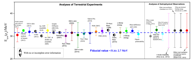
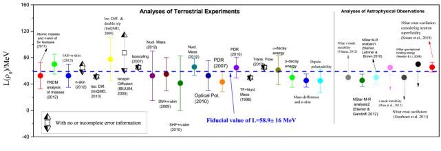
Figure 25: From Ref. Li et al. (2019). Constraints on saturation values of the symmetry energy (upper panel) and slope (lower panel) at saturation from terrestrial and astrophysical experiments.

In this section, we review various experiments to determine the symmetry energy parameters at saturation density. In Ref. Li et al. (2019), the authors illustrated a comprehensive list of $E_{sym}$ and $L$ at saturation density from 28 model assessments of terrestrial nuclear tests and astrophysical data with the fiducial values of (31.6$\pm$2.7) MeV and (58.9$\pm$16) MeV, respectively (see Fig. 25). The S$\pi$RIT collaboration from the Radioactive Isotope Beam Factory (RIBF) at RIKEN measured the spectra of charged pions produced by colliding rare isotope tin (Sn) beams with isotopically enriched Sn targets to restrict their contributions at suprasaturation densities. The calculated slope of the symmetry energy is (42 $<$ $L$ $<$ 117) MeV using ratios of charged pion spectra observed at high transverse momentum Estee et al. (2021). Furthermore, using the available experimental nuclear masses of heavy nuclei, $E_{sym}$ was determined, which was employed further to extract $L$=(50.0 $\pm$ 15.5) MeV at $n_{sat}$ = 0.16 fm^-3 Fan et al. (2014). As discussed earlier, the thickness of the neutron skin of ²⁰⁸Pb offers a strict laboratory restriction on the symmetry energy. Using the strong correlation between $R_{skin}$ and $L$, the updated Lead Radius Experiment (PREX-II) reported a large $L$=(106 $\pm$ 37) MeV based on both theoretical and actual data, consistently overestimating present limits Reed et al. (2021). In another PREX-II study, for ²⁰⁸Pb the parity-violating asymmetry $A_{PV}$ was studied using non-relativistic and relativistic energy density functionals Reinhard et al. (2021). A neutron skin thickness of $R^{208}_{skin}$=(0.19$\pm$0.02) fm, and a small value of derivative $L$=(54$\pm$8) MeV were obtained. These figures are in line with earlier astrophysical estimates and are considerably lower than those recently published using a specific set of relativistic energy density functionals.

VII.2.2 $E_{sym}$ and $L$ below saturation

Constraining the symmetry energy parameters at subsaturation density also helps to restrict the EoS of the neutron-star matter. Here, we discuss experimental measurements for $E_{sym}$ and $L$ below saturation density. The moderate-temperature nuclear gases formed in the collisions of ${}^{64}\mathrm{Zn}$ projectiles with ${}^{92}\mathrm{Mo}$ and ${}^{197}\mathrm{Au}$ target nuclei showed a large degree of $\alpha$ particle clustering at low densities. From isoscaling analyses of the yields of nuclei with $A\leq 4$, the temperature and density-dependent symmetry energy coefficients of these gases at densities $n_{B}=0.01~{}n_{sat}-0.05~{}n_{sat}$ were evaluated as $E_{sym}=9.03-13.6$ MeV (see table 1 of Kowalski et al. (2007)). From the measured excitation energies of the isovector giant quadrupole resonance (IVGQR) in ²⁰⁸Pb, the symmetry-energy value $E_{sym}=(23.3\pm 0.6)$ MeV at $n_{B}$ = 0.1 fm^-3 was estimated Roca-Maza et al. (2013). Furthermore, the magnitude of the symmetry energy $E_{\text{sym }}=(26.65\pm 0.20)$ MeV at a subsaturation cross density $n_{B}\approx 0.11$ fm^-3 was determined by the binding energy difference $\Delta E$ between a heavy isotope pair Zhang and Chen (2013). Using the available experimental nuclear masses of heavy nuclei $E_{sym,sat}$ was determined, which was employed further to extract the density dependent symmetry-energy value, $E_{sym}=(25.98\pm 0.01)$ MeV and the derivative, $L=(49.6\pm 6.2)$ MeV at $n_{B}$ = 0.11 fm^-3 Fan et al. (2014). The magnitude of the symmetry energy $E_{\text{sym }}$ at densities around $n_{sat}/3$ was determined uniquely by the electric dipole polarizability $\alpha_{\mathrm{D}}$ in ${}^{208}\mathrm{Pb}$. A stringent constraint of $E_{\mathrm{sym}}=(15.91\pm 0.99)$ MeV was observed at $n_{B}=0.05$ fm^-3 and for the range $n_{B}=0.02-0.11$ fm^-3, results are illustrated by the red band in Fig. 26 Zhang and Chen (2015). In addition, the nuclear symmetry coefficients were extracted using excitation energies to isobaric analog states (IAS) and charge invariance. A narrow constraint of $E_{sym}=$32.2 $\pm 2.4$ MeV was obtained at saturation and for the range of density $(0.04\lesssim n_{B}\lesssim 0.13)$ fm^-3, the behavior is illustrated in the left panel of Fig. 27. In addition, inclusion of the skin constraints narrows down the constraints for the same density range (see right panel of Fig. 27) and at saturation $E_{sym}$ becomes (32.2$\pm 1.1)$ MeV Danielewicz and Lee (2014). Table 7 summarizes the empirical constraints on $E_{sym}$ and $L$.

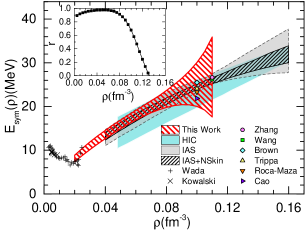
Figure 26: From Ref. Zhang and Chen (2015). Empirical constraints on symmetry energy vs baryon density.

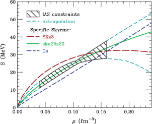
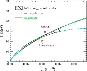
Figure 27: From Ref. Danielewicz and Lee (2014). Symmetry energy vs baryon density without (Left:) and with (Right:) neutron-skin constraints.

Constraints	Value	$n_{B}$	Reference
$E_{sym}$ (MeV)	31.6 $\pm$ 2.7	$n_{sat}$	Li et al. (2019)
	9.03 - 13.6	0.01-0.05 $n_{sat}$	Kowalski et al. (2007)
	15.91 $\pm$ 0.99	0.05 $n_{sat}$	Zhang and Chen (2015)
	23.3 $\pm$ 0.6	0.1 $n_{sat}$	Roca-Maza et al. (2013)
	26.65 $\pm$ 0.20	0.11 $n_{sat}$	Zhang and Chen (2013)
	25.98 $\pm$ 0.01	0.11 $n_{sat}$	Fan et al. (2014)
	32.20 $\pm$ 2.4	0.04 $\leq\frac{n_{B}}{n_{sat}}\leq$ 0.13	Danielewicz and Lee (2014)
$L$ (MeV)	58.16 $\pm$ 16	$n_{sat}$	Li et al. (2019)
	50 $\pm$ 15.5	$n_{sat}$	Fan et al. (2014)
	54 $\pm$ 8	$n_{sat}$	Reinhard et al. (2021)
	106 $\pm$ 37	$n_{sat}$	Reed et al. (2021)
	49.6 $\pm$ 6.2	0.11 $n_{sat}$	Fan et al. (2014)

Table 7: Empirical constraints related to isospin asymmetric matter for the symmetry energy and slope parameter.

VII.2.3 Correlation of symmetry energy and slope parameter

As discussed earlier, the symmetry energy and its slope play an important role in constraining the EoS of neutron-star matter. Thus, the correlation between both parameters can be useful to understand their interdependence. In Ref. Lattimer and Steiner (2014), authors illustrate the experimentally determined values of $E_{sym}$ and $L$ parameters. Fig. 28 contains different regimes coming from the observations of low-energy heavy-ion collisions, astrophysics, neutron skin, giant dipole resonance (GDR), isobaric analog states (IAS), and dipole polarizability.

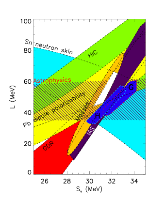
Figure 28: From Ref. Lattimer and Steiner (2014). Correlation between symmetry energy and slope at saturation.

VII.2.4 Heavy-ion collision measurements of neutron skin of ${}^{197}Au$ and ${}^{238}U$

Recently, from heavy-ion collisions it was discovered that it is possible to measure the nucleus charge radius by using the energy dependence of the Breit-Wheeler process Wang et al. (2022). Additionally, the STAR experiment has also found the total matter radius determined using the diffractive photoproduction in ultra-peripheral collisions to observe a unique spin interference pattern in the angular distribution of $\rho\rightarrow\pi^{+}+\pi^{-}$ decays Abdallah et al. (2023d). Combining these two measurements, they found that for ¹⁹⁷Au there was a neutron skin of $0.17\pm 0.03(stat.)\pm 0.08(syst.)$ fm and a for ²³⁸U there was a neutron skin of $0.44\pm 0.05(stat.)\pm 0.08(syst.)$ fm Abdallah et al. (2023d). To date these results have not yet been used in theoretical calculations but they do appear to be consistent with PREXII results.

VII.3 Isospin-symmetric nuclear matter liquid-gas critical point

The similarity between nucleon-nucleon and Van der Waals interactions suggested the possibility of also having a liquid-gas phase transition in nuclear matter if the effects of Coulomb and limited size are ignored. If that is the case, the existence of a coexistence line associated with a first order transition stopping at a critical point is expected. Indeed in the liquid-gas phase diagram, the surface tension of a nucleus diminishes as its temperature rises, eventually disappearing at a point known as the critical point Landau and Lifshitz (2000). The liquid-gas phase transition line divides two separate nuclear phases, i.e. nuclei (towards low density) and bulk matter (towards high density). In many models, if just nuclear matter is taken into account and Coulomb interactions are disregarded, this phase transition is anticipated as first-order Soma and Bozek (2009); Fiorilla et al. (2012) whereas in astrophysical environments, the production of nuclei involves the Coulomb and other interactions that occur in finite nuclei, where some characteristics of the first order phase transition may be retained Buyukcizmeci et al. (2013).

In this section, we review the different nuclear reaction experiments relevant to the liquid-gas phase diagram of symmetric nuclear matter. The critical temperature found in the studies on finite nuclei Karnaukhov et al. (2003); Elliott et al. (2013); Natowitz et al. (2002); Karnaukhov et al. (2008) is in the range $T_{c}\approx 17–20$ MeV. In a study from empirical observations of limiting temperatures, the critical temperature of infinite nuclear matter was found to be $T_{c}=16.6\pm 0.86\,$ MeV Natowitz et al. (2002). Also, in p $+$ Au collisions at 8.1 GeV, the charge distribution of the intermediate mass fragments was analyzed in the framework of the statistical multifragmentation model, and the critical temperature was found to be $T_{c}=20\pm 3\,$ MeV Karnaukhov et al. (2003). Furthermore, in another study, a critical temperature $T_{c}>15$ MeV was anticipated for the nuclear liquid-gas phase transition from fission and multifragmentation data (see Fig. 29 for a list of $T_{c}$ obtained from different studies Karnaukhov et al. (2008)). In the latest study, six different sets of experimental data obtained from the Lawrence Berkeley National Laboratory 88-inch cyclotron, Indiana Silicon Sphere Collaboration and Equation of State Collaboration indicated that infinite nuclear matter has critical rms values for temperature $(T_{c}=17.9\pm 0.4)\,$ MeV, density ${n_{B}}_{c}=(0.06\pm 0.01)\,$ fm^-3, and pressure $P_{c}=(0.31\pm 0.07)$, MeV fm^-3 Elliott et al. (2013). The critical temperature is essentially a parameter that affects how quickly the surface tension falls when the nuclei heat up. The values mentioned in this work are useful to constrain nuclear matter models at finite temperature. They are summarized in Table 8.

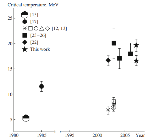
Figure 29: From Ref. Karnaukhov et al. (2008). Constraints on the critical temperature of the liquid-gas phase transition.

Constraints	Value	Reference
$T_{c}$ (MeV)	16.6 $\pm$ 0.86	Natowitz et al. (2002)
	20 $\pm$ 3	Karnaukhov et al. (2003)
	$>$15	Karnaukhov et al. (2008)
	17.9 $\pm$ 0.4	Elliott et al. (2013)
$P_{c}$ (MeV fm-3)	0.31 $\pm$ 0.07	Elliott et al. (2013)
${n_{B}}_{c}$ (fm-3)	0.06 $\pm$ 0.01	Elliott et al. (2013)

Table 8: Empirical constraints for the critical temperature, pressure, and baryon density related to liquid-gas critical point.

VIII Observational Constraints: Astrophysics

Measurements of stellar masses, radii and tidal deformabilities play a central role in establishing a link between neutron stars’ microscopic and macroscopic properties. These observables depend upon the internal structure and composition of the matter that makes up the neutron star. This microphysical information is relayed through the equations of stellar structure by the EoS, which cannot be directly measured in laboratory experiments at the densities, temperatures, and isospin asymmetries relevant for neutron star cores. In the astrophysical context, the EoS is probed by a variety of astronomical observations of neutron stars, particularly electromagnetic observations in the radio and X-ray bands, as well as gravitational waves from the coalescence of compact binaries.

Neutron stars, whether in isolation or in binaries systems, are described by the Einstein equations, which require, as input, the EoS to connect the pressure to the energy density and temperature inside the stars. When in isolation and when considering non-rotating stars, the Einstein equations reduce to the Tolman-Oppenheimer-Volkoff (TOV) equations Tolman (1939); Oppenheimer and Volkoff (1939), whose solution determines the mass and radius of the non-rotating star for a given central energy density. Choosing a sequence of central densities yields a sequence of pairs of masses and radii, which together form a “mass-radius curve.” For slowly-rotating stars, one can expand the Einstein equations in small rotation through the Hartle-Thorne approximation Hartle (1967), and the solution to the expanded equations yields the moment of inertia at first order in rotation, the quadrupole moment and a mass correction at second order. When a neutron star is not in isolation, but instead is perturbed by some external object (like a binary companion), the perturbations can also be studied by solving the linearized Einstein equations about a neutron star background, which yields the tidal deformabilities of the star. In this way, one can construct various curves, including the mass-radius, moment of inertia-mass, quadrupole moment-mass, tidal deformability-mass, and so on, that represent neutron stars of various central densities. These curves can change shape depending on the EoS prescribed. Since one usually expects neutron stars to all be described by a unique EoS , there is a single set of such curves that correctly describes Nature. Astrophysical observations can determine which set is the correct one, and thus, which is the correct EoS to describe neutron stars.

In the next subsections, we discuss one by one the empirical macroscopic constraints obtained from various astronomical observations. We provide summaries of current constraints with only brief explanations of the underlying measurements. See, e.g., Ref. Chatziioannou (2020) for a more thorough review.

It is important to remember that the densities relevant for the cores of neutron stars can certainly reach several times nuclear saturation density (see, e.g., Fig. 5 of Legred et al. (2021)), and connecting constraints from theoretical calculations and terrestrial experiments at lower densities (Secs. V and VII) to neutron star observations will almost certainly involve some extrapolation. The amount of freedom allowed in extrapolation schemes may be, but are not always, informed by physical models. Some care is, therefore, warranted when interpreting results combining low-density and high-density constraints as the conclusions often depend on the particular extrapolation scheme chosen. See, e.g., Refs. Essick et al. (2021a, b); Legred et al. (2022) for more discussion.

VIII.1 Neutron-star maximum mass

The measurement of a neutron star’s mass sets a lower bound on the mass above which the neutron star must undergo gravitational collapse to a black hole. Most observed neutron stars spin slowly compared with their Keplerian break-up rotation rate. Hence, mass observations are often used to bound the maximum mass achievable by cold, non-rotating neutron stars even though spin can support up to approximately $\sim 20\%$ additional mass Breu and Rezzolla (2016).

The record for the highest precisely and reliably measured neutron star mass currently belongs to the 2.8 ms radio pulsar (PSR) J0740+6620, which is likely orbiting an ultracool white dwarf companion Fonseca et al. (2021). The data sets of this study are integrated pulse arrival-time measurements, obtained using the Canadian Hydrogen Intensity Mapping Experiment (CHIME) and 100-meter Green Bank Telescope (GBT). Timing solutions for PSR J0740+6620 were produced by the GBT and CHIME/Pulsar collaborations using narrow-band and wide-band times of arrival. While comparing the credible intervals of the Shapiro delay parameters across different dispersion measures (DM) evolution models, all calculated solutions were found to be statistically compatible with different DMX models at 68.3$\%$ credibility, with a 1$\%$ fluctuation in the credible intervals of the Shapiro delay. The Shapiro delay, also known as the gravitational time delay effect, is an increase in travel time of a signal when it passes near a massive object. The estimated mass of PSR J0740+6620 is $m_{p}=2.08_{-0.07}^{+0.07}$ M_⊙ (in solar masses) and of its companion is $m_{c}=0.253_{-0.005}^{+0.006}$ M_⊙ Fonseca et al. (2021) calculated at $1\sigma$ (68.3$\%$ credibility), which is consistent with the earlier observations of Cromartie et al. Cromartie et al. (2019) (posterior in Ref. POS ).

The second-highest precisely and reliably measured pulsar mass belongs to PSR J0348+0432. For this pulsar, the mass is estimated to be $2.01\pm 0.04~{}M_{\odot}$ at 68.3% credibility based on a combination of radio timing of the pulsar and precise spectroscopy of the white dwarf companion, which has a mass of $m_{c}=0.173\pm 0.003~{}M_{\odot}$ and is in a 2.46-hour orbit around the pulsar Antoniadis et al. (2013).

An upper limit on the maximum mass of nonrotating neutron stars has been placed, albeit with more substantial astrophysical uncertainties, using the properties of short gamma-ray bursts. These have long been assumed to be produced by the merger of two neutron stars, with the remnant either forming a black hole immediately or collapsing quickly to a black hole (e.g., Murguia-Berthier et al. (2014)). Under this assumption, and working off of the mass distribution of double neutron star systems in our Galaxy, several authors proposed that the maximum mass $M_{\rm max}$ of a nonrotating neutron star was $\sim 2.3~{}M_{\odot}$ Bauswein et al. (2013); Lawrence et al. (2015); Fryer et al. (2015). The gravitational wave and electromagnetic data from the binary neutron-star merger GW170817, for which it was possible to make a good estimate of the total mass, also led to an estimate of $M_{\rm max}\sim 2.2-2.3~{}M_{\odot}$ Margalit and Metzger (2017). The argument for rapid collapse to a black hole is that otherwise the rapidly spinning remnant will spin down and inject energy into the remnant, which has not been seen. A key but unproven assumption in this argument is that the merger process will generate strong and ultimately poloidal magnetic fields that will spin down the remnant.

Detailed modeling of the electromagnetic afterglow of GW170817 has led to other estimates of the maximum mass, e.g., $M_{\mathrm{max}}\simeq 2.16^{+0.17}_{-0.15}M_{\odot}$ Rezzolla et al. (2018), M${}_{\mathrm{max}}\simeq 2.16–2.28M_{\odot}$ Ruiz et al. (2018), $M_{\mathrm{max}}\simeq 2.13^{+0.17}_{-0.11}M_{\odot}$ Shao et al. (2020), M${}_{\mathrm{max}}\lesssim 2.3$ M_⊙ Shibata et al. (2019), $M_{\mathrm{max}}\simeq 2.21^{+0.12}_{-0.12}M_{\odot}$ Nathanail et al. (2021), and if the assumption that the GW170817 event resulted in a black hole is relaxed, $M_{\mathrm{max}}\simeq 2.43^{+0.16}_{-0.12}M_{\odot}$ Ai et al. (2019). All of these estimates are subject to numerical and modeling uncertainties, but they are promising for the future. The empirical constraints on the maximum neutron-star mass are summarized in Table 9.

There have also been several claims of heavier neutron stars. The discovery of black-widow pulsars with masses estimated as $2.13\pm 0.04\,M_{\odot}$ Romani et al. (2021) for PSR J1810+1744 and $2.35\pm 0.17\,M_{\odot}$ Romani et al. (2022) (68% confidence) for PSR J0952-0607 have been reported; however, these mass measurements are less secure (due to possible systematics) than the Shapiro delay-based measurements for PSR J0740+6620 and PSR J0348+0432. Moreover, the $2.59^{+0.08}_{-0.09}\,M_{\odot}$ secondary component of the compact binary merger GW190814 has been touted as a potential heavy neutron star because it is less massive than known black holes Abbott et al. (2020b). However, its proximity in mass to the ostensible $2.7\,M_{\odot}$ black-hole remnant of GW170817, and the lack of any observed tidal effects or electromagnetic counterpart, have made people think that it may be more likely to be a black hole. However, this conclusion comes with some caveats. Tidal effects for such massive neutron stars are expected to be very small Tan et al. (2020), and in fact, not observable with the sensitivity of ground interferometers when this event was detected Abbott et al. (2020b). Moreover, the lack of an electromagnetic counterpart in the gamma range could be due to the short-gamma ray burst not being pointed toward Earth. An electromagnetic counterpart at other frequencies could have been missed due to the poor localization of the event in the sky through only the use of gravitational wave information. See Ref. de Sá et al. (2022) for a discussion on many candidates whose masses that lay inside the so called mass gap (between confirmed masses of neutron stars and black holes).

In another work, the authors used binary inclination $i$ from lightcurve modeling and observed that J1810 offers a lower limit on the NS maximum mass of $2M_{\odot}$ at 99.7 $\%$ credibility Romani et al. (2021). A flat, but asymmetric, light-curve maximum and a deep, narrow minimum were observed in the spectrophotometry of the companion of PSR J1810+1744 measured by the Keck telescope. A hot pole, surface winds, and severe gravity darkening (GD) around the $L_{1}$ point are all indicated by the maximum, whereas the minimum denotes significant limb darkening and a low underlying temperature. Having the radial-velocity amplitude $K_{\mathrm{c}}=462.3\pm 2.2$ km s^-1 recorded by the Keck telescope provides a precise neutron star mass of $M_{\mathrm{NS}}=2.13\pm 0.04M_{\odot}$, a value which is very relevant to the understanding of the dense-matter EoS Romani et al. (2021).

Neutron Star	Mmax (M⊙)	Reference
PSR J0740+6620	$\geq$ 2.08 $\pm$ 0.07	Fonseca et al. (2021)
PSR J0348+0432	$\geq$ 2.01 $\pm$ 0.04	Antoniadis et al. (2013)

Table 9: Pulsar empirical constraints on the maximum mass of neutron stars. Pulsar timing constraints are less susceptible to modeling assumptions than current gravitational wave constraints.

VIII.2 Neutron-star mass-radius regions from NICER

NICER is a soft X-ray telescope mounted on the International Space Station (ISS) in 2017. The main aim of NICER is to determine masses and radii of neutron stars using pulse-profile modeling of neighboring rotation-powered millisecond pulsars. The NICER observations have played an important role in lowering the ambiguity in the EoS of high-density matter (1.5–5 $n_{sat}$) at zero temperature. See Table 10 for a summary of the results reported from NICER, which we now discuss in detail. A word of warning is due at this stage: the results presented in this table (and in other tables in this section) are a summary, and in particular, the reported masses and radius with error bars are not a square in probability space. Rather, these quantities correspond to the maximum likelihood points and the 90% confidence regions of the marginalized posterior after a careful Bayesian parameter estimation study. Two-dimensional posteriors on mass and radius are not squares, but rather complicated shapes due to the correlation between parameters.

Neutron Star	M (M⊙)	Radius (km)	Reference
PSR J0030+0451	$1.34^{+0.15}_{-0.16}$	$12.71^{+1.14}_{-1.19}$	Riley et al. (2019)
PSR J0740+6620	$2.072^{+0.067}_{-0.066}$	$12.39^{+1.30}_{-1.98}$	Riley et al. (2021)
PSR J0030+0451	$1.44^{+0.15}_{-0.14}$	$13.02^{+1.24}_{-1.06}$	Miller et al. (2019)
PSR J0740+6620	$2.08^{+0.07}_{-0.07}$	$13.7^{+2.6}_{-1.5}$	Miller et al. (2021)

Table 10: Empirical constraints related to mass-radii from NICER.

Using Bayesian parameter estimation based on pulse-profile modeling of the NICER XTI event data for the isolated pulsar PSR J0030+0451, Miller et al. Miller et al. (2019) (posterior pos (a)) reported a gravitational mass $M=1.44^{+0.15}_{-0.14}~{}M_{\odot}$ and a circumferential radius $R=13.02^{+1.24}_{-1.06}$ km at $68\%$ credibility. For the same data but using slightly different models and a different statistical sampler, Riley et al. Riley et al. (2019) found $M=1.34^{+0.15}_{-0.16}~{}M_{\odot}$ and $R=12.71^{+1.14}_{-1.19}~{}{\rm km}$ (posterior pos (b) and raw data RAW ).

The heavy binary pulsar PSR J0740+6620 has a NICER count rate only $\sim 5$% that of PSR J0030+0451 and thus NICER data alone are insufficient for precise measurements of the mass and radius. As a result, for this pulsar, radio data and X-ray data from the X-ray Multi-Mirror (XMM-Newton) satellite were analyzed jointly with the NICER data. Miller et al. Miller et al. (2021) (posterior POS ) found $M=1.97-2.15~{}M_{\odot}$ and $R=12.21-16.33~{}{\rm km}$, both at 68% credibility, whereas Riley et al. Riley et al. (2021) (posterior pos ) reported $M=2.072^{+0.067}_{-0.066}~{}M_{\odot}$ and $R=12.39^{+1.30}_{-0.98}~{}{\rm km}$.

The differences between the two results for PSR J0740+6620 (e.g., Miller et al. report a $-1\sigma$ radius of 12.21 km, compared with Riley et al.’s estimate of 11.41 km) led the two groups to explore the reasons for the difference. As discussed in Miller et al. (2021), the primary differences are as follows. First, Miller et al. (2021) use a relative calibration between NICER and XMM-Newton that is consistent with the results of cross-calibration tests, whereas Riley et al. (2021) assume a much broader range of possible cross-calibration factors. When Riley et al. (2021) apply the same cross-calibration as Miller et al. (2021), they find a $-1\sigma$ radius of 11.75 km rather than 11.41 km, i.e., this accounts for almost half the difference from the 12.21 km $-1\sigma$ radius of Miller et al. (2021). Second, Riley et al. (2021) have a hard prior upper bound on the radius of 16 km, whereas Miller et al. (2021) allow the radius to be anything that fits the data. When Miller et al. (2021) eliminate all solutions with $R>16$ km, their $-1\sigma$ radius drops to 12.06 km. The remaining difference, of 0.31 km (compared with the original 0.8 km), is likely to be primarily due to different choices of statistical samplers: Miller et al. (2021) use the parallel-tempered Markov chain Monte Carlo code PT-emcee whereas Riley et al. (2021) use the nested sampler MultiNest; Miller et al. (2021) argue that at least in this specific case, MultiNest may underestimate the widths of the posteriors. More generally, there are many moving parts within such analyses and sometimes subtle choices on how data is analyzed or which data is analyzed can affect the resulting constraints; see Essick (2022) for an example related to data selection.

VIII.3 Other observational constraints on neutron star masses and radii

Quiescent low-mass X-ray binaries (QLMXBs) in globular clusters are promising objects for mass and radius constraints because (i) previous accretion events heat up the surface increasing their luminosity, (ii) their magnetic fields are expected (but not observed) to be relatively small, the magnetic field having been buried by the accretion, and (iii) the globular cluster permits a determination of the distance. There are several QLMXBs which have been used to obtain mass and radius constraints, see Ref. Steiner et al. (2018) for a recent analysis leading to neutron star radii between 10 and 14 km. However, there are still a significant number of potential systematics which may be important: (i) the magnetic field is not observed so the assumption of a small magnetic field is untested, (ii) the determination of the mass and radius requires a model of the neutron star atmosphere and the associated emergent X-ray spectrum, (iii) the composition of the accreted material is not always known, (iv) the temperature is often presumed to be uniform over the entire surface, and (v) scattering by the interstellar medium leads to a reddening of the spectrum which is not fully known. A recent attempt Al-Mamun et al. (2021) to search for systematic effects in QLMXB models compared QLMXBs to other mass and radius constraints (including those from LIGO/Virgo and NICER) and found no evidence for systematics that poison the QLMXB results. However, this result may change as the LIGO/Virgo constraints improve.

Within the supernova remnant HESS J1731-347, a star that is the centre compact object has been studied, according to the authors of Ref. Doroshenko et al. (2022), the mass and radius of this star is estimated to be $M=0.77_{-0.17}^{+0.20}M_{\odot}$ and $R=10.4_{-0.78}^{+0.86}\mathrm{~{}km}$, respectively, which is based on the modeling of Gaia observations and X-ray spectrum. This result depends critically on the assumption that the entire surface of the star emits at the same temperature, based on the lack of clear modulation with the stellar rotation. With that assumption, and the assumption that the atmospheric effects of the stellar magnetic field can be neglected, a carbon atmosphere is favored over a hydrogen or a helium atmosphere. However, as shown by Ref. Alford and Halpern (2023), nonuniform emission is consistent with the data on several similar sources (and preferred for some). This means that hydrogen and helium atmospheres are possible, and these could imply standard masses well above one solar mass. According to their estimation, this star can be either the lightest neutron star ever discovered or a strange star with exotic EoS Doroshenko et al. (2022). The examination of several SN explosions indicates that it is not feasible to form a neutron star (NS) with a mass less than approximately $1.17M_{\odot}$ Suwa et al. (2018), which begs the issue of what astronomical activity might result in such a small mass. Ref. Di Clemente et al. (2022) suggests that in the case of strange quark stars, masses of the order or less than one solar mass can be found and it is conceivable to construct a cogent astrophysical hypothesis that accounts for the object’s mass, radius, and gradual cooling.

VIII.4 Neutron-star tidal deformability from gravitational waves

The phasing of the gravitational waves emitted during the inspiral of a compact binary system is sensitive to the tidal deformation experienced by each component as a result of its companion’s non-uniform gravitational field. The size of the deformation is measured by the tidal deformability parameter Flanagan and Hinderer (2008); Hinderer (2008), which depends on the neutron-star mass and the EoS. The tidal deformabilities of the individual neutron stars appear at leading order in the gravitational waveform as a mass-weighted average known as the chirp or binary tidal deformability, $\tilde{\Lambda}$ Favata (2014); Wade et al. (2014), namely

$$\tilde{\Lambda}=\frac{16}{13}\left[\frac{(m_{1}+12m_{2})m_{1}^{4}\Lambda_{1}+(m_{2}+12m_{1})m_{2}^{4}\Lambda_{2}}{(m_{1}+m_{2})^{5}}\right]\ ,$$ (47)

where $m_{1}$ and $m_{2}$ are the masses of the binary components and $\Lambda_{1}$ and $\Lambda_{2}$ are their (dimensionless) individual tidal deformabilities. Because an EoS predicts a unique $m$–$\Lambda$ relation, a measurement of $\tilde{\Lambda}$ and the binary masses helps to determine the EoS in a manner analogous to constraints on the $m$–$R$ relation.

VIII.4.1 Extraction of $\tilde{\Lambda}$ from GW170817

The first measurement of $\tilde{\Lambda}$ was enabled by the detection of gravitational waves from the binary neutron-star merger GW170817 Abbott et al. (2017a) by LIGO and Virgo. The binary tidal deformability was constrained simultaneously with the system’s masses, spins and other source properties via Bayesian parameter estimation, in which a waveform model is compared against the data to produce a likelihood function over the waveform parameters (see e.g. Thrane and Talbot (2019)). Because the tidal deformability is mass-dependent, and gravitational-wave measurements of the binary mass ratio and spins are correlated, the constraints on $\tilde{\Lambda}$ are sensitive to prior assumptions about spin. Assuming that both neutron stars in GW170817 had low spins, in keeping with the Galactic double neutron-star population Burgay et al. (2003); Stovall et al. (2018), LIGO and Virgo measured $\tilde{\Lambda}=300^{+500}_{-190}$ at 90% confidence; without this assumption, the constraint is $\tilde{\Lambda}\leq 630$ Abbott et al. (2019). The joint constraints on $\tilde{\Lambda}$ and the binary masses are expressible in terms of a multi-dimensional posterior probability distribution, samples from which are available in the data release accompanying Abbott et al. (2019).

As before, a word of caution is due at this stage. The measurements of the tidal deformabilities discussed above and below in this section result from a Bayesian parameter estimation study, and as such, they correspond to the maximum likelihood points and the 90% confidence region of the marginalized posterior. The posterior is multi-dimensional and covariances exist between the various parameters that enter the waveform model. Therefore, 2-dimensional confidence regions, like that for the chirp tidal deformability and the chirp mass, are not squares, but rather complicated shapes, which can be found in the papers we have referenced here.

The analysis of the signal Abbott et al. (2019), and therefore, the tidal deformabilities reported above, do not require both of GW170817’s compact objects to share the same EoS, implicitly leaving open the possibility that one of them is a black hole. Because of the kilonova and short gamma-ray burst counterparts to GW170817, however, it is reasonable to assume that the merger consisted of two neutron stars De et al. (2018). The assumption that all neutron stars share the same EoS implicitly relates $\Lambda_{1}$ and $\Lambda_{2}$, since the EoS predicts a unique $m$–$\Lambda$ relation. The authors of Ref. De et al. (2018) approximated this relation as $\Lambda_{1}=\Lambda_{2}{m_{2}}^{6}/{m_{1}}^{6}$, and used it to further constrain $\tilde{\Lambda}=222^{+420}_{-138}$ at 90% confidence, assuming low neutron-star spins. An alternative to making such an approximation is to average over many different candidate EoSs drawn from a prior distribution: each EoS sample imposes an exact relation between $\Lambda_{1}$ and $\Lambda_{2}$, and the EoS uncertainty encoded in the prior distribution is propagated to $\tilde{\Lambda}$ by the averaging process. Of course, this approach requires modeling the EoS. Typically, this is done phenomenologically, either with a parameterization of the pressure-density relation (e.g a spectral decomposition Lindblom (2010)) or with a Gaussian process Landry and Essick (2019) (i.e. a distribution over functions described by a mean function and a covariance kernel). Caveats exist here, however, because the choice of the functional form of the EoS may not include the entire phase space of possible equations of state that can be conceived from nuclear physics.

The EoS-averaging approach was taken by Ref. Essick et al. (2020), which modeled the EoS nonparametrically as a Gaussian process and found $\tilde{\Lambda}=245^{+361}_{-160}$ (posterior median and 90% highest-probability-density credible region). The Gaussian process was constructed to explore the entire functional space of EoSs that obey causality (sound speed less than the speed of light) and thermodynamic stability (positive semidenfinite sound speed), subject to the requirement that the EoS support neutron star masses of at least $1.93\,M_{\odot}$ to account for the existence of heavy pulsars. For comparison, when using a spectral parameterization for the EoS, one find $\tilde{\Lambda}=412^{+313}_{-262}$ for the posterior median and 90% credible regions. If one instead uses the global maximum of the posterior, one finds $\tilde{\Lambda}=225^{+500}_{-75}$, which is similar to that found using Gaussian processes.

Electromagnetic observations of GW170817’s kilonova counterpart have also been used to constrain the binary tidal deformability. However, these bounds depend on the assumed kilonova lightcurve model and are thus subject to sizeable systematic uncertainty: for example, $\tilde{\Lambda}\geq 197$ (90% confidence) Coughlin et al. (2018), $120<\tilde{\Lambda}<1110$ (90% confidence) Breschi et al. (2021), and $109\leq\tilde{\Lambda}\leq 137$ (68% confidence) Nicholl et al. (2021) was found. Unlike the gravitational-wave measurements of binary tidal deformability, $\tilde{\Lambda}$ does not appear directly as a parameter in the light curve model and it must therefore be constrained via correlations with other observables. As discussed in Radice et al. (2018), these constraints come with the possibility of large errors associated with uncertainties in the mass ratio of the system Kiuchi et al. (2019).

VIII.4.2 Extraction of individual tidal deformabilities $\Lambda_{1}$ and $\Lambda_{2}$

The binary tidal deformability $\tilde{\Lambda}$ is the tidal parameter that is best constrained by gravitational-wave observations. However, it is the individual tidal deformability $\Lambda$ that is directly determined by the EoS together with the equations of stellar structure. The relation between the individual tidal deformabilities $\Lambda_{1}$ and $\Lambda_{2}$ of each member of a compact binary and the system’s binary tidal deformability is expressed in Eq. (47). Generally, the component masses $m_{1}$ and $m_{2}$ are constrained simultaneously with $\tilde{\Lambda}$ through the Bayesian parameter estimation of the gravitational-wave signal. Thus, we have one equation relating three tidal parameters: a measurement of $\tilde{\Lambda}$ only determines $\Lambda_{1}$ and $\Lambda_{2}$ up to a residual degeneracy. This degeneracy is broken by a tidal parameter $\delta\tilde{\Lambda}$ that appears at higher order in the gravitational waveform, but it is unfortunately not measurable with current detectors Wade et al. (2014).

Nonetheless, this degeneracy is not an obstacle to translating measurements of $\tilde{\Lambda}$ into constraints on $\Lambda_{1}$ and $\Lambda_{2}$: it is simply the case that every combination of $\Lambda_{1}$ and $\Lambda_{2}$ that produces the same $\tilde{\Lambda}$ is equally likely. Thus, one can build up a posterior for $\Lambda_{1}$ and $\Lambda_{2}$ by sampling in the individual tidal deformabilities, and assigning to each sample the likelihood of the $\tilde{\Lambda}$ it predicts (the likelihood is the ratio of the posterior probability to the prior probability). The result of this process for GW170817 is the posterior on the component tidal deformabilities illustrated in Fig. 10 of Ref. Abbott et al. (2019); notice that there is a direction in $\Lambda_{1}$–$\Lambda_{2}$ plane along which there is essentially no constraint due to the degeneracy.

One can break the degeneracy by introducing an additional layer of modeling that imposes a common EoS for both components of GW170817: this augments Eq. (47) with a second equation relating the individual tidal deformabilities. As in the case of $\tilde{\Lambda}$, this can be done either with an approximate relation connecting $\Lambda_{1}$ and $\Lambda_{2}$, or by averaging over an EoS prior distribution.

Using the Gaussian process-based EoS representation described above, Ref. Essick et al. (2020) mapped the binary tidal deformability measurement into constraints of $\Lambda_{1}=148^{+274}_{-125}$ and $\Lambda_{2}=430^{+519}_{-301}$ on the component tidal deformabilities, under the assumption of low neutron-star spins. Moreover, since each EoS sample from the Gaussian process prescribes an exact $m$–$\Lambda$ relation, this approach allows the tidal deformability to be inferred at any mass scale. Reference Essick et al. (2020) also constrained $\Lambda_{1.4}=211^{+312}_{-137}$ (posterior median and 90% highest-probability-density credible region).

Alternatively, one can break the degeneracy with an approximate EoS-insensitive relation connecting the individual tidal deformabilities. The so-called binary Love relations Yagi and Yunes (2016) fit the relation between two independent linear combinations of $\Lambda_{1}$ and $\Lambda_{2}$ to many candidate EoSs from nuclear theory. With the neutron stars’ individual tidal deformabilities related by way of this EoS-insensitive relation Chatziioannou et al. (2018), augmented with Gaussian white noise to account for the scatter in the fit, and $\Lambda$’s mass dependence expanded in a series about $1.4\,M_{\odot}$, Abbott et al. (2018) reduced the joint constraint on binary masses and $\tilde{\Lambda}$ from GW170817 to an estimate of the tidal deformability of a $1.4\,M_{\odot}$ neutron star: $\Lambda_{1.4}=190^{+390}_{-120}$ at the $90\%$ credible level, in the low neutron-star spin scenario. The empirical constraints on the tidal deformability from GW170817 are summarized in Table 11.

Tidal deformability	Reference	Confidence level
$\tilde{\Lambda}=300^{+500}_{-190}$	low spins Abbott et al. (2019)	$90\%$
$\tilde{\Lambda}\leq 630$	minimal assumptions Abbott et al. (2019)	$90\%$
$\tilde{\Lambda}=222^{+420}_{-138}$	common EoS via analytic approximation De et al. (2018)	$90\%$
$\Lambda_{1.4}=190^{+390}_{-120}$	common EoS via binary Love relation Abbott et al. (2018)	$90\%$
$\tilde{\Lambda}=245^{+361}_{-160}$	common EoS via Gaussian process Essick et al. (2020)	$90\%$
$\Lambda_{1.4}=211^{+312}_{-137}$	common EoS via Gaussian process Essick et al. (2020)	$90\%$

Table 11: Empirical constraints on the tidal deformability for GW170817 event from LIGO and VIRGO.

The results for the extracted tidal deformability posteriors from GW170817 are shown in Fig. 30. While there is a lot of overlap for the posteriors of the EoS insensitive (universal relations), spectral EoS, and Gaussian Process EoS, they are not exactly the same and this may lead to incorrect conclusions when extracting the EoS unless one is careful. For instance, most nuclear physics EoS tend towards higher values of $\Lambda$ for a given M. Thus, the EoS insensitive posterior may seem more restricting than the spectral EoS. However, since these are 90% confidence regions, all posteriors are actually statistically consistent with each other, and one cannot simply take the edge of one posterior to draw strong conclusions without a careful Bayesian parameter estimation study.

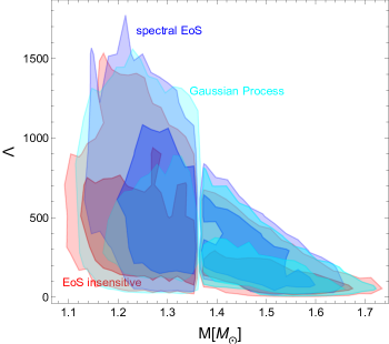
Figure 30: Constraints on the tidal deformability using the universal relations (EOS insensitive), the spectral EOS and an EoS constructed from Gaussian Processes. The universal-relation constraint and spectral-EoS constraint are obtained using GW170817 data. The Gaussian Process constraint is obtained by combining GW170817, PSR 1614-2230, PSR 0348+0432, and PSR 0740+6620 (mass only) data. Shaded regions are shown at the $68\%$ and $95\%$ confidence regions.

VIII.4.3 Connecting tidal deformabilities to the mass-radius sequence

Because the neutron-star tidal deformability scales strongly with the stellar radius ($\Lambda\sim R^{5}/m^{5}$), and because $R$ is an easily interpretable parameter, gravitational-wave measurements of $\Lambda$ have often been translated into radius constraints in the literature. Nonetheless, we stress that gravitational waves from compact binaries do not directly measure the neutron star radius—the mapping from $\Lambda$ to $R$ necessarily involves additional modeling. This modeling can either be done at the level of the EoS (e.g. with a spectral or nonparametric EoS representation), or at the level of the mapping itself (e.g. with an EoS-insensitive relation between $\Lambda$ and the stellar compactness $m/R$).

In Ref. Abbott et al. (2018), LIGO and Virgo mapped the joint posterior on component tidal deformabilities and masses from GW170817 (assuming a binary Love relation) into a posterior on $m_{1}$, $m_{2}$, $R_{1}$ and $R_{2}$ by adopting a spectral parameterization for the EoS. The original posterior was used to compute the likelihood of each spectral EoS realization, and then for each component mass sample from the original posterior, the radius predicted by the EoS realization’s mass-radius relation was assigned that likelihood. This procedure led to inferred radii of $R_{1}=11.9^{+1.4}_{-1.4}$ km and $R_{2}=11.9^{+1.4}_{-1.4}$ km.

LIGO and Virgo also implented an alternative approach that used an EoS-insensitive $\Lambda$–$m/R$ relation. For each component mass and component tidal deformability sample from the original posterior, $\Lambda$ was mapped to $m/R$ using the relation from Ref. Yagi and Yunes (2017), and the radius was extracted using the sampled mass. The uncertainty in the EoS-insensitive relation fit was modeled as Gaussian white noise in the relation. This procedure led to inferred radii of $R_{1}=10.8^{2.0}_{-1.7}$ km and $R_{2}=10.7^{2.1}_{-1.5}$ km. The small differences vs the radius constraints with the spectral EoSs illustrate the systematic uncertainty that arises from the extra modeling required.

In Ref. De et al. (2018), a different EoS-insensitive relation was used to map from the tidal deformability measurement to a radius constraint. Imposing the common EoS assumption $\Lambda_{1}=\Lambda_{2}{m_{2}}^{6}/{m_{1}}^{6}$ described above and assuming that both neutron stars involved in GW170817 had the same radius $R$, the definition of the binary tidal deformability reduces to $\tilde{\Lambda}\propto(R/\mathcal{M})^{6}$, with an EoS-insensitive constant of proportionality that can be fit to a sample of various EoSs. The joint posterior on $\tilde{\Lambda}$ and $\mathcal{M}$ from GW170817 thus determines the common neutron-star radius, which was reported as $R=10.7^{+2.1}_{-1.6}$ km at 90% confidence.

A summary of the resulting mass-radius constraints from both NICER and GW170817 can be see in Fig. 31. The heavier NICER pulsar (J0740+6620) has the highest posterior distribution that is centered nearly directly above the lighter NICER pulsar (J0030+0451) and the GW170817 extracted mass-radius posteriors. However, there is some probability that heavier $M\sim 2M_{\odot}$ may bend to the right. The lighter constraints from J0030+0451 and GW170817 overlap in their posteriors as well, although GW170817 generally prefers a slightly smaller radius whereas J0030+0451’s posterior prefers larger radii.

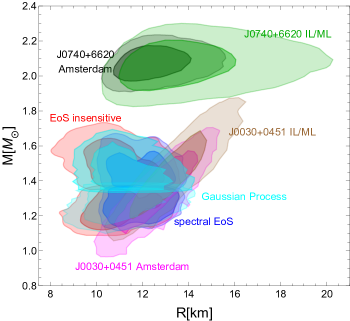
Figure 31: Constraints on the mass-radius using the universal relations (EOS insensitive), the spectral EOS and an EoS sampled through Gaussian Processes. The universal-relation constraint and spectral-EoS constraint are obtained using GW170817 data. The Gaussian Process constraint is obtained by combining GW170817, PSR 1614-2230, PSR 0348+0432, and PSR 0740+6620 (mass only) data. NICER constraints from both the Amsterdam and Illinois/Maryland groups are show for both J0030+0451 and J0740+6620. Shaded regions show the $68\%$ and $95\%$ confidence region.

Different methods (EoS insensitive, spectral EoS and Gaussian processes) to obtain the posterior on the mass and radius with GW170817 may look different, but they all are statistically consistent with each other. In particular, we stress that one cannot use these posteriors, over-impose mass-radius curves computed with a given EoS and then determine whether the EoS is allowed or disallowed based on whether it overlaps with the contours or not. This is because each point on this plane, including those outside the 68% or the 95% confidence regions, actually has a posterior weight assigned to it (not shown in the figure). Therefore, comparison of the data to a given EoS needs to be done carefully in a Bayesian way. Overall, all posteriors are statistically consistent with each other at this time, and therefore, there is no tension between observations. Eventually, if future observations place better constraints on the mass-radius plane, one expects that a single EoS will be preferred by all data.

We emphasize that these radius constraints from GW170817 are merely approximate encapsulations of the information contained within the tidal deformability measurements reported above, which are directly constrained by the gravitational waves. When considering gravitational wave data, it is thus preferable to use the tidal deformability measurements to constrain the EoS.

VIII.4.4 GW190425, GW200105, and GW200115

Gravitational waves also yielded a constraint on tidal deformability in the binary neutron-star merger GW190425, but because this system was heavier (such that its $\tilde{\Lambda}$ is intrinsically smaller) and more distant (such that its signal-to-noise ratio was lower), the constraint is not competitive with GW170817. Similarly, GW200105 and GW200115 Abbott et al. (2021) both likely contained neutron stars, but tidal effects were unmeasureably small in these systems due to the large masses of their companions and subsequent rapid orbital evolution through GW emission.

IX Outlook

In this work, we compiled various constraints coming from nuclear and astrophysics related to dense matter and neutron stars. We encapsulated up to date results from first principle theories and experimental observations. The usage of anticipated next-generation facilities and theoretical advancements are the most promising path for substantial improvement above current limitations. With enhanced sensitivity and expanded receiver bandwidths, several upcoming astrophysical radio observatories, including the dish Deep Synoptic Array, DSA-2000 Hallinan et al. (2019), Canadian Hydrogen Observatory and Radio-transient Detector, CHORD Vanderlinde et al. (2019), and the next-generation Very Large Array, ngVLA Chatterjee (2018), will present significant opportunities in pulsar science. Also, we anticipate seeing more multi-messenger binary neutron-star merger detections in the coming years, the INTEGRAL, Fermi, Swift, and SVOM will observe merging binary neutron stars in conjunction with GW and electromagnetic data during the fourth LIGO-Virgo-KAGRA observing run expected to start on May of 2023 Patricelli et al. (2022). Future detections of neutrinos from supernova explosions in our neighborhood will provide information about larger $Y_{Q}$ at large densities and intermediate temperatures, while with future LIGO and NICER runs the post-merger signal of gravitation waves from neutron-star mergers will provide information about low $Y_{Q}$ at large densities and large temperatures Lovato et al. (2022).

Several improvements are anticipated in the next phase of BES, thanks to the performance enhancements brought on by collider and detector modifications which will help to dig deeper into the high density regime of the QCD phase diagram. Constraining the EoS is not a simple task and significant work from different communities in nuclear and astrophysics is needed to achieve this. Within the nuclear physics community, the diverse models and theories, working in a different regime of QCD phase diagram are to be updated with the modern constraints so that we can have a unified EoS for nuclei, bulk baryonic and quark matter.

References

- Gross and Wilczek (1973) D. J. Gross and F. Wilczek, Phys. Rev. Lett. 30, 1343 (1973).
- Politzer (1973) H. D. Politzer, Phys. Rev. Lett. 30, 1346 (1973).
- Aaij et al. (2019) R. Aaij et al. (LHCb), Phys. Rev. Lett. 122, 222001 (2019), arXiv:1904.03947 [hep-ex] .
- Workman et al. (2022) R. L. Workman et al. (Particle Data Group), PTEP 2022, 083C01 (2022).
- Citron et al. (2019) Z. Citron et al., CERN Yellow Rep. Monogr. 7, 1159 (2019), arXiv:1812.06772 [hep-ph] .
- STARcollaboration (2014) STARcollaboration, “Studying the Phase Diagram of QCD Matter at RHIC,” (2014).
- Cebra et al. (2014) D. Cebra, S. G. Brovko, C. E. Flores, B. A. Haag, and J. L. Klay, (2014), arXiv:1408.1369 [nucl-ex] .
- Pianese et al. (2018) S. Pianese et al., in 9th International Particle Accelerator Conference (2018).
- Galatyuk (2014) T. Galatyuk (HADES), Nucl. Phys. A 931, 41 (2014).
- Galatyuk (2020) T. Galatyuk (HADES), JPS Conf. Proc. 32, 010079 (2020).
- Friese (2006) V. Friese, Nucl. Phys. A 774, 377 (2006).
- Tahir et al. (2005) N. A. Tahir et al., Phys. Rev. Lett. 95, 035001 (2005).
- Lutz et al. (2009a) M. F. M. Lutz et al. (PANDA), (2009a), arXiv:0903.3905 [hep-ex] .
- Durante et al. (2019) M. Durante et al., Phys. Scripta 94, 033001 (2019), arXiv:1903.05693 [nucl-th] .
- Dexheimer et al. (2021a) V. Dexheimer, J. Noronha, J. Noronha-Hostler, C. Ratti, and N. Yunes, J. Phys. G 48, 073001 (2021a), arXiv:2010.08834 [nucl-th] .
- Lovato et al. (2022) A. Lovato et al., (2022), arXiv:2211.02224 [nucl-th] .
- Sorensen et al. (2023) A. Sorensen et al., (2023), arXiv:2301.13253 [nucl-th] .
- Joglekar et al. (2020) A. Joglekar, N. Raj, P. Tanedo, and H.-B. Yu, Phys. Rev. D 102, 123002 (2020), arXiv:2004.09539 [hep-ph] .
- Blaschke et al. (2020) D. Blaschke, H. Grigorian, and G. Röpke, Particles 3, 477 (2020), arXiv:2005.10218 [nucl-th] .
- (20) “https://compstar.uni-frankfurt.de/outreach/short-articles/the-hyperon-puzzle/,” https://compstar.uni-frankfurt.de/outreach/short-articles/the-hyperon-puzzle/, accessed: 2022-06-04.
- Bednarek et al. (2012) I. Bednarek, P. Haensel, J. L. Zdunik, M. Bejger, and R. Manka, Astron. Astrophys. 543, A157 (2012), arXiv:1111.6942 [astro-ph.SR] .
- Buballa et al. (2014) M. Buballa et al., J. Phys. G 41, 123001 (2014), arXiv:1402.6911 [astro-ph.HE] .
- Rijken and Schulze (2016) T. A. Rijken and H. J. Schulze, Eur. Phys. J. A 52, 21 (2016).
- Lonardoni et al. (2015) D. Lonardoni, A. Lovato, S. Gandolfi, and F. Pederiva, Phys. Rev. Lett. 114, 092301 (2015), arXiv:1407.4448 [nucl-th] .
- Gerstung et al. (2020) D. Gerstung, N. Kaiser, and W. Weise, Eur. Phys. J. A 56, 175 (2020), arXiv:2001.10563 [nucl-th] .
- Bodmer (1991) A. R. Bodmer, Nucl. Phys. A 526, 703 (1991).
- Dexheimer et al. (2021b) V. Dexheimer, R. O. Gomes, T. Klähn, S. Han, and M. Salinas, Phys. Rev. C 103, 025808 (2021b), arXiv:2007.08493 [astro-ph.HE] .
- Hagedorn (1983) R. Hagedorn, Z. Phys. C 17, 265 (1983).
- Dexheimer et al. (2013) V. Dexheimer, J. Steinheimer, R. Negreiros, and S. Schramm, Phys. Rev. C 87, 015804 (2013), arXiv:1206.3086 [astro-ph.HE] .
- Vidana et al. (2005) I. Vidana, I. Bombaci, and I. Parenti, Nucl. Phys. A 754, 345 (2005).
- Weissenborn et al. (2012) S. Weissenborn, D. Chatterjee, and J. Schaffner-Bielich, Phys. Rev. C 85, 065802 (2012), [Erratum: Phys.Rev.C 90, 019904 (2014)], arXiv:1112.0234 [astro-ph.HE] .
- Glendenning (1985) N. K. Glendenning, Astrophys. J. 293, 470 (1985).
- Schürhoff et al. (2010) T. Schürhoff, S. Schramm, and V. Dexheimer, Astrophys. J. Lett. 724, L74 (2010), arXiv:1008.0957 [astro-ph.SR] .
- Drago et al. (2014) A. Drago, A. Lavagno, G. Pagliara, and D. Pigato, Phys. Rev. C 90, 065809 (2014), arXiv:1407.2843 [astro-ph.SR] .
- Li et al. (2018) J. J. Li, A. Sedrakian, and F. Weber, Phys. Lett. B 783, 234 (2018), arXiv:1803.03661 [nucl-th] .
- Marquez et al. (2022) K. D. Marquez, M. R. Pelicer, S. Ghosh, J. Peterson, D. Chatterjee, V. Dexheimer, and D. P. Menezes, Phys. Rev. C 106, 035801 (2022), arXiv:2205.09827 [astro-ph.HE] .
- Dexheimer et al. (2021c) V. Dexheimer, K. D. Marquez, and D. P. Menezes, Eur. Phys. J. A 57, 216 (2021c), arXiv:2103.09855 [nucl-th] .
- Troyer and Wiese (2005) M. Troyer and U.-J. Wiese, Phys. Rev. Lett. 94, 170201 (2005), arXiv:cond-mat/0408370 .
- Borsányi et al. (2021) S. Borsányi, Z. Fodor, J. N. Guenther, R. Kara, S. D. Katz, P. Parotto, A. Pásztor, C. Ratti, and K. K. Szabó, Phys. Rev. Lett. 126, 232001 (2021), arXiv:2102.06660 [hep-lat] .
- Borsanyi et al. (2022) S. Borsanyi, J. N. Guenther, R. Kara, Z. Fodor, P. Parotto, A. Pasztor, C. Ratti, and K. K. Szabo, Phys. Rev. D 105, 114504 (2022), arXiv:2202.05574 [hep-lat] .
- Alba et al. (2017) P. Alba et al., Phys. Rev. D 96, 034517 (2017), arXiv:1702.01113 [hep-lat] .
- Bellwied et al. (2020) R. Bellwied, S. Borsanyi, Z. Fodor, J. N. Guenther, J. Noronha-Hostler, P. Parotto, A. Pasztor, C. Ratti, and J. M. Stafford, Phys. Rev. D 101, 034506 (2020), arXiv:1910.14592 [hep-lat] .
- Andersen et al. (2010a) J. O. Andersen, M. Strickland, and N. Su, Phys. Rev. Lett. 104, 122003 (2010a), arXiv:0911.0676 [hep-ph] .
- Andersen et al. (2010b) J. O. Andersen, M. Strickland, and N. Su, JHEP 08, 113 (2010b), arXiv:1005.1603 [hep-ph] .
- Andersen et al. (2011a) J. O. Andersen, L. E. Leganger, M. Strickland, and N. Su, Phys. Lett. B 696, 468 (2011a), arXiv:1009.4644 [hep-ph] .
- Andersen et al. (2011b) J. O. Andersen, L. E. Leganger, M. Strickland, and N. Su, Phys. Rev. D 84, 087703 (2011b), arXiv:1106.0514 [hep-ph] .
- Mogliacci et al. (2013) S. Mogliacci, J. O. Andersen, M. Strickland, N. Su, and A. Vuorinen, JHEP 12, 055 (2013), arXiv:1307.8098 [hep-ph] .
- Haque et al. (2014a) N. Haque, J. O. Andersen, M. G. Mustafa, M. Strickland, and N. Su, Phys. Rev. D 89, 061701 (2014a), arXiv:1309.3968 [hep-ph] .
- Haque et al. (2014b) N. Haque, A. Bandyopadhyay, J. O. Andersen, M. G. Mustafa, M. Strickland, and N. Su, JHEP 05, 027 (2014b), arXiv:1402.6907 [hep-ph] .
- Haque and Strickland (2021) N. Haque and M. Strickland, Phys. Rev. C 103, 031901 (2021), arXiv:2011.06938 [hep-ph] .
- Ghiglieri et al. (2020) J. Ghiglieri, A. Kurkela, M. Strickland, and A. Vuorinen, Phys. Rept. 880, 1 (2020), arXiv:2002.10188 [hep-ph] .
- Andersen and Strickland (2002) J. O. Andersen and M. Strickland, Phys. Rev. D 66, 105001 (2002), arXiv:hep-ph/0206196 .
- Komoltsev and Kurkela (2022) O. Komoltsev and A. Kurkela, Phys. Rev. Lett. 128, 202701 (2022), arXiv:2111.05350 [nucl-th] .
- Braaten and Nieto (1995) E. Braaten and A. Nieto, Phys. Rev. D 51, 6990 (1995), arXiv:hep-ph/9501375 .
- Braaten and Nieto (1996a) E. Braaten and A. Nieto, Phys. Rev. D 53, 3421 (1996a), arXiv:hep-ph/9510408 .
- Andersen et al. (2002) J. O. Andersen, E. Braaten, E. Petitgirard, and M. Strickland, Phys. Rev. D 66, 085016 (2002), arXiv:hep-ph/0205085 .
- Andersen et al. (2004) J. O. Andersen, E. Petitgirard, and M. Strickland, Phys. Rev. D 70, 045001 (2004), arXiv:hep-ph/0302069 .
- Freedman and McLerran (1977a) B. A. Freedman and L. D. McLerran, Phys. Rev. D 16, 1130 (1977a).
- Freedman and McLerran (1977b) B. A. Freedman and L. D. McLerran, Phys. Rev. D 16, 1147 (1977b).
- Freedman and McLerran (1977c) B. A. Freedman and L. D. McLerran, Phys. Rev. D 16, 1169 (1977c).
- Gorda et al. (2018) T. Gorda, A. Kurkela, P. Romatschke, M. Säppi, and A. Vuorinen, Phys. Rev. Lett. 121, 202701 (2018), arXiv:1807.04120 [hep-ph] .
- Gorda et al. (2021a) T. Gorda, A. Kurkela, R. Paatelainen, S. Säppi, and A. Vuorinen, Phys. Rev. Lett. 127, 162003 (2021a), arXiv:2103.05658 [hep-ph] .
- Gorda et al. (2021b) T. Gorda, A. Kurkela, R. Paatelainen, S. Säppi, and A. Vuorinen, Phys. Rev. D 104, 074015 (2021b), arXiv:2103.07427 [hep-ph] .
- Weinberg (1979) S. Weinberg, Physica A 96, 327 (1979).
- Epelbaum et al. (2009) E. Epelbaum, H.-W. Hammer, and U.-G. Meissner, Rev. Mod. Phys. 81, 1773 (2009), arXiv:0811.1338 [nucl-th] .
- Machleidt and Entem (2011) R. Machleidt and D. R. Entem, Phys. Rept. 503, 1 (2011), arXiv:1105.2919 [nucl-th] .
- Drischler et al. (2021a) C. Drischler, J. W. Holt, and C. Wellenhofer, Ann. Rev. Nucl. Part. Sci. 71, 403 (2021a), arXiv:2101.01709 [nucl-th] .
- Hebeler et al. (2010) K. Hebeler, J. M. Lattimer, C. J. Pethick, and A. Schwenk, Phys. Rev. Lett. 105, 161102 (2010), arXiv:1007.1746 [nucl-th] .
- Sammarruca et al. (2015) F. Sammarruca, L. Coraggio, J. W. Holt, N. Itaco, R. Machleidt, and L. E. Marcucci, Phys. Rev. C 91, 054311 (2015), arXiv:1411.0136 [nucl-th] .
- Tews et al. (2018) I. Tews, J. Carlson, S. Gandolfi, and S. Reddy, Astrophys. J. 860, 149 (2018), arXiv:1801.01923 [nucl-th] .
- Drischler et al. (2020) C. Drischler, R. J. Furnstahl, J. A. Melendez, and D. R. Phillips, Phys. Rev. Lett. 125, 202702 (2020), arXiv:2004.07232 [nucl-th] .
- Nambu and Jona-Lasinio (1961a) Y. Nambu and G. Jona-Lasinio, Phys. Rev. 122, 345 (1961a).
- Nambu and Jona-Lasinio (1961b) Y. Nambu and G. Jona-Lasinio, Phys. Rev. 124, 246 (1961b).
- Hatsuda and Kunihiro (1994) T. Hatsuda and T. Kunihiro, Phys. Rept. 247, 221 (1994), arXiv:hep-ph/9401310 .
- Dexheimer and Schramm (2010) V. A. Dexheimer and S. Schramm, Phys. Rev. C 81, 045201 (2010), arXiv:0901.1748 [astro-ph.SR] .
- Motornenko et al. (2020) A. Motornenko, J. Steinheimer, V. Vovchenko, S. Schramm, and H. Stoecker, Phys. Rev. C 101, 034904 (2020), arXiv:1905.00866 [hep-ph] .
- Rougemont et al. (2017) R. Rougemont, R. Critelli, J. Noronha-Hostler, J. Noronha, and C. Ratti, Phys. Rev. D 96, 014032 (2017), arXiv:1704.05558 [hep-ph] .
- Critelli et al. (2017) R. Critelli, J. Noronha, J. Noronha-Hostler, I. Portillo, C. Ratti, and R. Rougemont, Phys. Rev. D 96, 096026 (2017), arXiv:1706.00455 [nucl-th] .
- Grefa et al. (2021) J. Grefa, J. Noronha, J. Noronha-Hostler, I. Portillo, C. Ratti, and R. Rougemont, Phys. Rev. D 104, 034002 (2021), arXiv:2102.12042 [nucl-th] .
- Grefa et al. (2022) J. Grefa, M. Hippert, J. Noronha, J. Noronha-Hostler, I. Portillo, C. Ratti, and R. Rougemont, Phys. Rev. D 106, 034024 (2022), arXiv:2203.00139 [nucl-th] .
- Adamczyk et al. (2017) L. Adamczyk et al. (STAR), Phys. Rev. C 96, 044904 (2017), arXiv:1701.07065 [nucl-ex] .
- Strickland (1994) M. Strickland, Phys. Lett. B 331, 245 (1994).
- Schenke and Strickland (2007) B. Schenke and M. Strickland, Phys. Rev. D 76, 025023 (2007), arXiv:hep-ph/0611332 .
- Martinez and Strickland (2008) M. Martinez and M. Strickland, Phys. Rev. C 78, 034917 (2008), arXiv:0805.4552 [hep-ph] .
- Dion et al. (2011) M. Dion, J.-F. Paquet, B. Schenke, C. Young, S. Jeon, and C. Gale, Phys. Rev. C 84, 064901 (2011), arXiv:1109.4405 [hep-ph] .
- Shen et al. (2014) C. Shen, U. W. Heinz, J.-F. Paquet, and C. Gale, Phys. Rev. C 89, 044910 (2014), arXiv:1308.2440 [nucl-th] .
- Gale et al. (2015) C. Gale, Y. Hidaka, S. Jeon, S. Lin, J.-F. Paquet, R. D. Pisarski, D. Satow, V. V. Skokov, and G. Vujanovic, Phys. Rev. Lett. 114, 072301 (2015), arXiv:1409.4778 [hep-ph] .
- Bhattacharya et al. (2016) L. Bhattacharya, R. Ryblewski, and M. Strickland, Phys. Rev. D 93, 065005 (2016), arXiv:1507.06605 [hep-ph] .
- Ryblewski and Strickland (2015) R. Ryblewski and M. Strickland, Phys. Rev. D 92, 025026 (2015), arXiv:1501.03418 [nucl-th] .
- Paquet et al. (2016) J.-F. Paquet, C. Shen, G. S. Denicol, M. Luzum, B. Schenke, S. Jeon, and C. Gale, Phys. Rev. C 93, 044906 (2016), arXiv:1509.06738 [hep-ph] .
- Kasmaei and Strickland (2019) B. S. Kasmaei and M. Strickland, Phys. Rev. D 99, 034015 (2019), arXiv:1811.07486 [hep-ph] .
- Kasmaei and Strickland (2020) B. S. Kasmaei and M. Strickland, Phys. Rev. D 102, 014037 (2020), arXiv:1911.03370 [hep-ph] .
- Stephanov (2009) M. A. Stephanov, Phys. Rev. Lett. 102, 032301 (2009), arXiv:0809.3450 [hep-ph] .
- Parotto et al. (2020) P. Parotto, M. Bluhm, D. Mroczek, M. Nahrgang, J. Noronha-Hostler, K. Rajagopal, C. Ratti, T. Schäfer, and M. Stephanov, Phys. Rev. C 101, 034901 (2020), arXiv:1805.05249 [hep-ph] .
- Mroczek et al. (2021) D. Mroczek, A. R. Nava Acuna, J. Noronha-Hostler, P. Parotto, C. Ratti, and M. A. Stephanov, Phys. Rev. C 103, 034901 (2021), arXiv:2008.04022 [nucl-th] .
- Adam et al. (2021a) J. Adam et al. (STAR), Phys. Rev. Lett. 126, 092301 (2021a), arXiv:2001.02852 [nucl-ex] .
- Abdallah et al. (2023a) M. Abdallah et al. (STAR), Phys. Rev. C 107, 024908 (2023a), arXiv:2209.11940 [nucl-ex] .
- Adamczewski-Musch et al. (2020a) J. Adamczewski-Musch et al. (HADES), Phys. Rev. C 102, 024914 (2020a), arXiv:2002.08701 [nucl-ex] .
- Acharya et al. (2020a) S. Acharya et al. (ALICE), Phys. Lett. B 807, 135564 (2020a), arXiv:1910.14396 [nucl-ex] .
- Abdallah et al. (2021a) M. Abdallah et al. (STAR), Phys. Rev. Lett. 127, 262301 (2021a), arXiv:2105.14698 [nucl-ex] .
- STA (2022) (2022), arXiv:2209.08058 [nucl-ex] .
- Tlusty (2018) D. Tlusty, in 13th Conference on the Intersections of Particle and Nuclear Physics (2018) arXiv:1810.04767 [nucl-ex] .
- Spies (2022) S. Spies (HADES), EPJ Web Conf. 259, 01007 (2022).
- Lutz et al. (2009b) M. F. M. Lutz et al. (PANDA), (2009b), arXiv:0903.3905 [hep-ex] .
- Bluhm et al. (2020) M. Bluhm et al., Nucl. Phys. A 1003, 122016 (2020), arXiv:2001.08831 [nucl-th] .
- Danielewicz et al. (2002) P. Danielewicz, R. Lacey, and W. G. Lynch, Science 298, 1592 (2002), arXiv:nucl-th/0208016 .
- Spieles and Bleicher (2020) C. Spieles and M. Bleicher, Eur. Phys. J. ST 229, 3537 (2020), arXiv:2006.01220 [nucl-th] .
- Schäfer et al. (2022) A. Schäfer, I. Karpenko, X.-Y. Wu, J. Hammelmann, and H. Elfner, Eur. Phys. J. A 58, 230 (2022), arXiv:2112.08724 [hep-ph] .
- Shen and Schenke (2022) C. Shen and B. Schenke, Phys. Rev. C 105, 064905 (2022), arXiv:2203.04685 [nucl-th] .
- Oliinychenko et al. (2022) D. Oliinychenko, A. Sorensen, V. Koch, and L. McLerran, (2022), arXiv:2208.11996 [nucl-th] .
- Raduta et al. (2021) A. R. Raduta, F. Nacu, and M. Oertel, Eur. Phys. J. A 57, 329 (2021), arXiv:2109.00251 [nucl-th] .
- Raduta (2022) A. R. Raduta, Eur. Phys. J. A 58, 115 (2022), arXiv:2205.03177 [nucl-th] .
- Constantinou et al. (2015) C. Constantinou, B. Muccioli, M. Prakash, and J. M. Lattimer, Phys. Rev. C 92, 025801 (2015), arXiv:1504.03982 [astro-ph.SR] .
- Raithel et al. (2019) C. A. Raithel, F. Ozel, and D. Psaltis, Astrophys. J. 875, 12 (2019), arXiv:1902.10735 [astro-ph.HE] .
- Elliott et al. (2012) J. B. Elliott, P. T. Lake, L. G. Moretto, and L. Phair, (2012), arXiv:1203.5132 [nucl-ex] .
- Tolman (1939) R. C. Tolman, Phys. Rev. 55, 364 (1939).
- Oppenheimer and Volkoff (1939) J. R. Oppenheimer and G. M. Volkoff, Phys. Rev. 55, 374 (1939).
- Demorest et al. (2010) P. Demorest, T. Pennucci, S. Ransom, M. Roberts, and J. Hessels, Nature 467, 1081 (2010), arXiv:1010.5788 [astro-ph.HE] .
- Gendreau et al. (2016) K. C. Gendreau, Z. Arzoumanian, P. W. Adkins, C. L. Albert, J. F. Anders, A. T. Aylward, C. L. Baker, E. R. Balsamo, W. A. Bamford, S. S. Benegalrao, D. L. Berry, S. Bhalwani, J. K. Black, C. Blaurock, G. M. Bronke, G. L. Brown, J. G. Budinoff, J. D. Cantwell, T. Cazeau, P. T. Chen, T. G. Clement, A. T. Colangelo, J. S. Coleman, J. D. Coopersmith, W. E. Dehaven, J. P. Doty, M. D. Egan, T. Enoto, T. W.-M. Fan, D. M. Ferro, R. Foster, N. M. Galassi, L. D. Gallo, C. M. Green, D. Grosh, K. Q. Ha, M. A. Hasouneh, K. B. Heefner, P. Hestnes, L. J. Hoge, T. M. Jacobs, J. L. Jørgensen, M. A. Kaiser, J. W. Kellogg, S. J. Kenyon, R. G. Koenecke, R. P. Kozon, B. LaMarr, M. D. Lambertson, A. M. Larson, S. Lentine, J. H. Lewis, M. G. Lilly, K. A. Liu, A. Malonis, S. S. Manthripragada, C. B. Markwardt, B. D. Matonak, I. E. Mcginnis, R. L. Miller, A. L. Mitchell, J. W. Mitchell, J. S. Mohammed, C. A. Monroe, K. M. M. de Garcia, P. D. Mulé, L. T. Nagao, S. N. Ngo, E. D. Norris, D. A. Norwood, J. Novotka, T. Okajima, L. G. Olsen, C. O. Onyeachu, H. Y. Orosco, J. R. Peterson, K. N. Pevear, K. K. Pham, S. E. Pollard, J. S. Pope, D. F. Powers, C. E. Powers, S. R. Price, G. Y. Prigozhin, J. B. Ramirez, W. J. Reid, R. A. Remillard, E. M. Rogstad, G. P. Rosecrans, J. N. Rowe, J. A. Sager, C. A. Sanders, B. Savadkin, M. R. Saylor, A. F. Schaeffer, N. S. Schweiss, S. R. Semper, P. J. Serlemitsos, L. V. Shackelford, Y. Soong, J. Struebel, M. L. Vezie, J. S. Villasenor, L. B. Winternitz, G. I. Wofford, M. R. Wright, M. Y. Yang, and W. H. Yu, in Space Telescopes and Instrumentation 2016: Ultraviolet to Gamma Ray, Vol. 9905, edited by J.-W. A. den Herder, T. Takahashi, and M. Bautz, International Society for Optics and Photonics (SPIE, 2016) pp. 420 – 435.
- Baubock et al. (2015) M. Baubock, D. Psaltis, and F. Ozel, Astrophys. J. 811, 144 (2015), arXiv:1505.00780 [astro-ph.HE] .
- Miller (2016) M. C. Miller, Astrophys. J. 822, 27 (2016), arXiv:1602.00312 [astro-ph.HE] .
- Ozel et al. (2016) F. Ozel, D. Psaltis, Z. Arzoumanian, S. Morsink, and M. Baubock, Astrophys. J. 832, 92 (2016), arXiv:1512.03067 [astro-ph.HE] .
- Abbott et al. (2017a) B. P. Abbott et al. (LIGO Scientific, Virgo), Phys. Rev. Lett. 119, 161101 (2017a), arXiv:1710.05832 [gr-qc] .
- Abbott et al. (2017b) B. P. Abbott et al. (LIGO Scientific, Virgo, Fermi GBM, INTEGRAL, IceCube, AstroSat Cadmium Zinc Telluride Imager Team, IPN, Insight-Hxmt, ANTARES, Swift, AGILE Team, 1M2H Team, Dark Energy Camera GW-EM, DES, DLT40, GRAWITA, Fermi-LAT, ATCA, ASKAP, Las Cumbres Observatory Group, OzGrav, DWF (Deeper Wider Faster Program), AST3, CAASTRO, VINROUGE, MASTER, J-GEM, GROWTH, JAGWAR, CaltechNRAO, TTU-NRAO, NuSTAR, Pan-STARRS, MAXI Team, TZAC Consortium, KU, Nordic Optical Telescope, ePESSTO, GROND, Texas Tech University, SALT Group, TOROS, BOOTES, MWA, CALET, IKI-GW Follow-up, H.E.S.S., LOFAR, LWA, HAWC, Pierre Auger, ALMA, Euro VLBI Team, Pi of Sky, Chandra Team at McGill University, DFN, ATLAS Telescopes, High Time Resolution Universe Survey, RIMAS, RATIR, SKA South Africa/MeerKAT), Astrophys. J. Lett. 848, L12 (2017b), arXiv:1710.05833 [astro-ph.HE] .
- Annala et al. (2018) E. Annala, T. Gorda, A. Kurkela, and A. Vuorinen, Phys. Rev. Lett. 120, 172703 (2018), arXiv:1711.02644 [astro-ph.HE] .
- Baym et al. (2018) G. Baym, T. Hatsuda, T. Kojo, P. D. Powell, Y. Song, and T. Takatsuka, Rept. Prog. Phys. 81, 056902 (2018), arXiv:1707.04966 [astro-ph.HE] .
- Antoniadis et al. (2013) J. Antoniadis et al., Science 340, 6131 (2013), arXiv:1304.6875 [astro-ph.HE] .
- Cromartie et al. (2019) H. T. Cromartie et al. (NANOGrav), Nature Astron. 4, 72 (2019), arXiv:1904.06759 [astro-ph.HE] .
- Fonseca et al. (2021) E. Fonseca et al., Astrophys. J. Lett. 915, L12 (2021), arXiv:2104.00880 [astro-ph.HE] .
- Miller et al. (2019) M. C. Miller et al., Astrophys. J. Lett. 887, L24 (2019), arXiv:1912.05705 [astro-ph.HE] .
- Riley et al. (2019) T. E. Riley et al., Astrophys. J. Lett. 887, L21 (2019), arXiv:1912.05702 [astro-ph.HE] .
- Miller et al. (2021) M. C. Miller et al., Astrophys. J. Lett. 918, L28 (2021), arXiv:2105.06979 [astro-ph.HE] .
- Riley et al. (2021) T. E. Riley et al., Astrophys. J. Lett. 918, L27 (2021), arXiv:2105.06980 [astro-ph.HE] .
- Abbott et al. (2018) B. P. Abbott et al. (LIGO Scientific, Virgo), Phys. Rev. Lett. 121, 161101 (2018), arXiv:1805.11581 [gr-qc] .
- Abbott et al. (2019) B. P. Abbott et al. (LIGO Scientific, Virgo), Phys. Rev. X 9, 011001 (2019), arXiv:1805.11579 [gr-qc] .
- Abbott et al. (2020a) B. P. Abbott et al. (LIGO Scientific, Virgo), Astrophys. J. Lett. 892, L3 (2020a), arXiv:2001.01761 [astro-ph.HE] .
- Bauswein et al. (2017) A. Bauswein, O. Just, H.-T. Janka, and N. Stergioulas, Astrophys. J. Lett. 850, L34 (2017), arXiv:1710.06843 [astro-ph.HE] .
- Margalit and Metzger (2017) B. Margalit and B. D. Metzger, Astrophys. J. Lett. 850, L19 (2017), arXiv:1710.05938 [astro-ph.HE] .
- Radice et al. (2018) D. Radice, A. Perego, F. Zappa, and S. Bernuzzi, Astrophys. J. Lett. 852, L29 (2018), arXiv:1711.03647 [astro-ph.HE] .
- Rezzolla et al. (2018) L. Rezzolla, E. R. Most, and L. R. Weih, Astrophys. J. Lett. 852, L25 (2018), arXiv:1711.00314 [astro-ph.HE] .
- Ruiz et al. (2018) M. Ruiz, S. L. Shapiro, and A. Tsokaros, Phys. Rev. D 97, 021501 (2018), arXiv:1711.00473 [astro-ph.HE] .
- Shibata et al. (2017) M. Shibata, S. Fujibayashi, K. Hotokezaka, K. Kiuchi, K. Kyutoku, Y. Sekiguchi, and M. Tanaka, Phys. Rev. D 96, 123012 (2017), arXiv:1710.07579 [astro-ph.HE] .
- Carson et al. (2019) Z. Carson, K. Chatziioannou, C.-J. Haster, K. Yagi, and N. Yunes, Phys. Rev. D 99, 083016 (2019), arXiv:1903.03909 [gr-qc] .
- Adamczewski-Musch et al. (2019a) J. Adamczewski-Musch et al. (HADES), Nature Phys. 15, 1040 (2019a).
- Alford et al. (2018) M. G. Alford, L. Bovard, M. Hanauske, L. Rezzolla, and K. Schwenzer, Phys. Rev. Lett. 120, 041101 (2018), arXiv:1707.09475 [gr-qc] .
- Alford et al. (2019) M. Alford, A. Harutyunyan, and A. Sedrakian, Phys. Rev. D 100, 103021 (2019), arXiv:1907.04192 [astro-ph.HE] .
- Alford and Harris (2019) M. G. Alford and S. P. Harris, Phys. Rev. C 100, 035803 (2019), arXiv:1907.03795 [nucl-th] .
- Alford et al. (2021) M. Alford, A. Harutyunyan, and A. Sedrakian, Phys. Rev. D 104, 103027 (2021), arXiv:2108.07523 [astro-ph.HE] .
- Gavassino et al. (2021) L. Gavassino, M. Antonelli, and B. Haskell, Class. Quant. Grav. 38, 075001 (2021), arXiv:2003.04609 [gr-qc] .
- Celora et al. (2022) T. Celora, I. Hawke, P. C. Hammond, N. Andersson, and G. L. Comer, Phys. Rev. D 105, 103016 (2022), arXiv:2202.01576 [astro-ph.HE] .
- Most et al. (2022) E. R. Most, A. Haber, S. P. Harris, Z. Zhang, M. G. Alford, and J. Noronha, (2022), arXiv:2207.00442 [astro-ph.HE] .
- Drischler et al. (2021b) C. Drischler, W. Haxton, K. McElvain, E. Mereghetti, A. Nicholson, P. Vranas, and A. Walker-Loud, Prog. Part. Nucl. Phys. 121, 103888 (2021b), arXiv:1910.07961 [nucl-th] .
- Borsanyi et al. (2014a) S. Borsanyi, Z. Fodor, C. Hoelbling, S. D. Katz, S. Krieg, and K. K. Szabo, Phys. Lett. B 730, 99 (2014a), arXiv:1309.5258 [hep-lat] .
- Bazavov et al. (2014) A. Bazavov et al. (HotQCD), Phys. Rev. D 90, 094503 (2014), arXiv:1407.6387 [hep-lat] .
- Aoki et al. (2006) Y. Aoki, Z. Fodor, S. D. Katz, and K. K. Szabo, JHEP 01, 089 (2006), arXiv:hep-lat/0510084 .
- Borsanyi et al. (2010) S. Borsanyi, G. Endrodi, Z. Fodor, A. Jakovac, S. D. Katz, S. Krieg, C. Ratti, and K. K. Szabo, JHEP 11, 077 (2010), arXiv:1007.2580 [hep-lat] .
- Ratti (2018) C. Ratti, Rept. Prog. Phys. 81, 084301 (2018), arXiv:1804.07810 [hep-lat] .
- Guenther et al. (2017) J. N. Guenther, R. Bellwied, S. Borsanyi, Z. Fodor, S. D. Katz, A. Pasztor, C. Ratti, and K. K. Szabó, Nucl. Phys. A 967, 720 (2017), arXiv:1607.02493 [hep-lat] .
- Bazavov et al. (2017) A. Bazavov et al., Phys. Rev. D 95, 054504 (2017), arXiv:1701.04325 [hep-lat] .
- Bollweg et al. (2022) D. Bollweg, J. Goswami, O. Kaczmarek, F. Karsch, S. Mukherjee, P. Petreczky, C. Schmidt, and P. Scior (HotQCD), Phys. Rev. D 105, 074511 (2022), arXiv:2202.09184 [hep-lat] .
- Alba et al. (2014) P. Alba, W. Alberico, R. Bellwied, M. Bluhm, V. Mantovani Sarti, M. Nahrgang, and C. Ratti, Phys. Lett. B 738, 305 (2014), arXiv:1403.4903 [hep-ph] .
- Borsanyi et al. (2012) S. Borsanyi, Z. Fodor, S. D. Katz, S. Krieg, C. Ratti, and K. Szabo, JHEP 01, 138 (2012), arXiv:1112.4416 [hep-lat] .
- Bellwied et al. (2015) R. Bellwied, S. Borsanyi, Z. Fodor, S. D. Katz, A. Pasztor, C. Ratti, and K. K. Szabo, Phys. Rev. D 92, 114505 (2015), arXiv:1507.04627 [hep-lat] .
- Borsanyi et al. (2018) S. Borsanyi, Z. Fodor, J. N. Guenther, S. K. Katz, K. K. Szabo, A. Pasztor, I. Portillo, and C. Ratti, JHEP 10, 205 (2018), arXiv:1805.04445 [hep-lat] .
- Bellwied et al. (2013) R. Bellwied, S. Borsanyi, Z. Fodor, S. D. Katz, and C. Ratti, Phys. Rev. Lett. 111, 202302 (2013), arXiv:1305.6297 [hep-lat] .
- Bazavov et al. (2013a) A. Bazavov et al., Phys. Rev. Lett. 111, 082301 (2013a), arXiv:1304.7220 [hep-lat] .
- Borsanyi et al. (2020) S. Borsanyi, Z. Fodor, J. N. Guenther, R. Kara, S. D. Katz, P. Parotto, A. Pasztor, C. Ratti, and K. K. Szabo, Phys. Rev. Lett. 125, 052001 (2020), arXiv:2002.02821 [hep-lat] .
- Bazavov et al. (2019a) A. Bazavov et al. (HotQCD), Phys. Lett. B 795, 15 (2019a), arXiv:1812.08235 [hep-lat] .
- Ding et al. (2019) H. T. Ding et al. (HotQCD), Phys. Rev. Lett. 123, 062002 (2019), arXiv:1903.04801 [hep-lat] .
- Braaten and Pisarski (1990a) E. Braaten and R. D. Pisarski, Nucl. Phys. B 337, 569 (1990a).
- Braaten and Pisarski (1990b) E. Braaten and R. D. Pisarski, Phys. Rev. Lett. 64, 1338 (1990b).
- Braaten and Pisarski (1990c) E. Braaten and R. D. Pisarski, Phys. Rev. D 42, 2156 (1990c).
- Arnold and Zhai (1994) P. B. Arnold and C.-X. Zhai, Phys. Rev. D 50, 7603 (1994), arXiv:hep-ph/9408276 .
- Arnold and Zhai (1995) P. B. Arnold and C.-x. Zhai, Phys. Rev. D 51, 1906 (1995), arXiv:hep-ph/9410360 .
- Zhai and Kastening (1995) C.-x. Zhai and B. M. Kastening, Phys. Rev. D 52, 7232 (1995), arXiv:hep-ph/9507380 .
- Kajantie et al. (1997) K. Kajantie, M. Laine, K. Rummukainen, and M. E. Shaposhnikov, Nucl. Phys. B 503, 357 (1997), arXiv:hep-ph/9704416 .
- Andersen et al. (1999) J. O. Andersen, E. Braaten, and M. Strickland, Phys. Rev. Lett. 83, 2139 (1999), arXiv:hep-ph/9902327 .
- Andersen et al. (2000a) J. O. Andersen, E. Braaten, and M. Strickland, Phys. Rev. D 61, 014017 (2000a), arXiv:hep-ph/9905337 .
- Andersen et al. (2000b) J. O. Andersen, E. Braaten, and M. Strickland, Phys. Rev. D 61, 074016 (2000b), arXiv:hep-ph/9908323 .
- Blaizot et al. (1999a) J. P. Blaizot, E. Iancu, and A. Rebhan, Phys. Rev. Lett. 83, 2906 (1999a), arXiv:hep-ph/9906340 .
- Blaizot et al. (1999b) J. P. Blaizot, E. Iancu, and A. Rebhan, Phys. Lett. B 470, 181 (1999b), arXiv:hep-ph/9910309 .
- Blaizot et al. (2001a) J. P. Blaizot, E. Iancu, and A. Rebhan, Phys. Rev. D 63, 065003 (2001a), arXiv:hep-ph/0005003 .
- Blaizot et al. (2001b) J. P. Blaizot, E. Iancu, and A. Rebhan, Phys. Lett. B 523, 143 (2001b), arXiv:hep-ph/0110369 .
- Andersen et al. (2011c) J. O. Andersen, L. E. Leganger, M. Strickland, and N. Su, JHEP 08, 053 (2011c), arXiv:1103.2528 [hep-ph] .
- Kurkela et al. (2014) A. Kurkela, E. S. Fraga, J. Schaffner-Bielich, and A. Vuorinen, Astrophys. J. 789, 127 (2014), arXiv:1402.6618 [astro-ph.HE] .
- Shuryak (1978) E. V. Shuryak, Sov. Phys. JETP 47, 212 (1978).
- Braaten and Nieto (1996b) E. Braaten and A. Nieto, Phys. Rev. Lett. 76, 1417 (1996b), arXiv:hep-ph/9508406 .
- Toimela (1985) T. Toimela, Int. J. Theor. Phys. 24, 901 (1985), [Erratum: Int.J.Theor.Phys. 26, 1021 (1987)].
- Kapusta (1979) J. I. Kapusta, Nucl. Phys. B 148, 461 (1979).
- Annala et al. (2020) E. Annala, T. Gorda, A. Kurkela, J. Nättilä, and A. Vuorinen, Nature Phys. 16, 907 (2020), arXiv:1903.09121 [astro-ph.HE] .
- Kurkela et al. (2010) A. Kurkela, P. Romatschke, and A. Vuorinen, Phys. Rev. D 81, 105021 (2010), arXiv:0912.1856 [hep-ph] .
- Borsanyi (2013) S. Borsanyi, Nucl. Phys. A 904-905, 270c (2013), arXiv:1210.6901 [hep-lat] .
- Borsanyi et al. (2013) S. Borsanyi, Z. Fodor, S. D. Katz, S. Krieg, C. Ratti, and K. K. Szabo, Phys. Rev. Lett. 111, 062005 (2013), arXiv:1305.5161 [hep-lat] .
- Bazavov et al. (2013b) A. Bazavov, H. T. Ding, P. Hegde, F. Karsch, C. Miao, S. Mukherjee, P. Petreczky, C. Schmidt, and A. Velytsky, Phys. Rev. D 88, 094021 (2013b), arXiv:1309.2317 [hep-lat] .
- Cea et al. (2016) P. Cea, L. Cosmai, and A. Papa, Phys. Rev. D 93, 014507 (2016), arXiv:1508.07599 [hep-lat] .
- Bonati et al. (2015) C. Bonati, M. D’Elia, M. Mariti, M. Mesiti, F. Negro, and F. Sanfilippo, Phys. Rev. D 92, 054503 (2015), arXiv:1507.03571 [hep-lat] .
- Bonati et al. (2018) C. Bonati, M. D’Elia, F. Negro, F. Sanfilippo, and K. Zambello, Phys. Rev. D 98, 054510 (2018), arXiv:1805.02960 [hep-lat] .
- Bazavov et al. (2019b) A. Bazavov et al. (HotQCD), Phys. Lett. B 795, 15 (2019b), arXiv:1812.08235 [hep-lat] .
- Shen et al. (1998) H. Shen, H. Toki, K. Oyamatsu, and K. Sumiyoshi, Nucl. Phys. A 637, 435 (1998), arXiv:nucl-th/9805035 .
- Kurkela and Vuorinen (2016) A. Kurkela and A. Vuorinen, Phys. Rev. Lett. 117, 042501 (2016), arXiv:1603.00750 [hep-ph] .
- Baluni (1978) V. Baluni, Phys. Rev. D 17, 2092 (1978).
- Vuorinen (2003) A. Vuorinen, Phys. Rev. D 68, 054017 (2003), arXiv:hep-ph/0305183 .
- Marczenko et al. (2023) M. Marczenko, L. McLerran, K. Redlich, and C. Sasaki, Phys. Rev. C 107, 025802 (2023), arXiv:2207.13059 [nucl-th] .
- Somasundaram et al. (2022) R. Somasundaram, I. Tews, and J. Margueron, (2022), arXiv:2204.14039 [nucl-th] .
- Meyer (2011) H. B. Meyer, Eur. Phys. J. A 47, 86 (2011), arXiv:1104.3708 [hep-lat] .
- Denicol and Rischke (2021) G. Denicol and D. H. Rischke, Microscopic Foundations of Relativistic Fluid Dynamics (Springer, 2021).
- Ghiglieri et al. (2018a) J. Ghiglieri, G. D. Moore, and D. Teaney, JHEP 03, 179 (2018a), arXiv:1802.09535 [hep-ph] .
- Ghiglieri et al. (2018b) J. Ghiglieri, G. D. Moore, and D. Teaney, Phys. Rev. Lett. 121, 052302 (2018b), arXiv:1805.02663 [hep-ph] .
- Danhoni and Moore (2023) I. Danhoni and G. D. Moore, JHEP 02, 124 (2023), arXiv:2212.02325 [hep-ph] .
- Liao and Koch (2010) J. Liao and V. Koch, Phys. Rev. C 81, 014902 (2010), arXiv:0909.3105 [hep-ph] .
- Arnold et al. (2006) P. B. Arnold, C. Dogan, and G. D. Moore, Phys. Rev. D 74, 085021 (2006), arXiv:hep-ph/0608012 .
- Arnold et al. (2000) P. B. Arnold, G. D. Moore, and L. G. Yaffe, JHEP 11, 001 (2000), arXiv:hep-ph/0010177 .
- York and Moore (2009) M. A. York and G. D. Moore, Phys. Rev. D 79, 054011 (2009), arXiv:0811.0729 [hep-ph] .
- Denicol et al. (2012) G. S. Denicol, H. Niemi, E. Molnar, and D. H. Rischke, Phys. Rev. D 85, 114047 (2012), [Erratum: Phys.Rev.D 91, 039902 (2015)], arXiv:1202.4551 [nucl-th] .
- Denicol et al. (2014) G. S. Denicol, S. Jeon, and C. Gale, Phys. Rev. C 90, 024912 (2014), arXiv:1403.0962 [nucl-th] .
- Kovtun et al. (2005) P. Kovtun, D. T. Son, and A. O. Starinets, Phys. Rev. Lett. 94, 111601 (2005), arXiv:hep-th/0405231 .
- Finazzo et al. (2015) S. I. Finazzo, R. Rougemont, H. Marrochio, and J. Noronha, JHEP 02, 051 (2015), arXiv:1412.2968 [hep-ph] .
- Everett et al. (2021) D. Everett et al. (JETSCAPE), Phys. Rev. C 103, 054904 (2021), arXiv:2011.01430 [hep-ph] .
- Drischler et al. (2014) C. Drischler, V. Soma, and A. Schwenk, Phys. Rev. C 89, 025806 (2014), arXiv:1310.5627 [nucl-th] .
- Wellenhofer et al. (2016) C. Wellenhofer, J. W. Holt, and N. Kaiser, Phys. Rev. C 93, 055802 (2016), arXiv:1603.02935 [nucl-th] .
- Wen and Holt (2021) P. Wen and J. W. Holt, Phys. Rev. C 103, 064002 (2021), arXiv:2012.02163 [nucl-th] .
- Somasundaram et al. (2021) R. Somasundaram, C. Drischler, I. Tews, and J. Margueron, Phys. Rev. C 103, 045803 (2021), arXiv:2009.04737 [nucl-th] .
- Lim and Holt (2017) Y. Lim and J. W. Holt, Phys. Rev. C 95, 065805 (2017), arXiv:1702.02898 [nucl-th] .
- Grams et al. (2022) G. Grams, J. Margueron, R. Somasundaram, and S. Reddy, Eur. Phys. J. A 58, 56 (2022), arXiv:2203.11645 [nucl-th] .
- Lim et al. (2021) Y. Lim, A. Bhattacharya, J. W. Holt, and D. Pati, Phys. Rev. C 104, L032802 (2021), arXiv:2007.06526 [nucl-th] .
- Drischler et al. (2021c) C. Drischler, S. Han, J. M. Lattimer, M. Prakash, S. Reddy, and T. Zhao, Phys. Rev. C 103, 045808 (2021c), arXiv:2009.06441 [nucl-th] .
- Brandes et al. (2023) L. Brandes, W. Weise, and N. Kaiser, Phys. Rev. D 107, 014011 (2023), arXiv:2208.03026 [nucl-th] .
- Holt and Kaiser (2017) J. W. Holt and N. Kaiser, Phys. Rev. C 95, 034326 (2017), arXiv:1612.04309 [nucl-th] .
- Drischler et al. (2019) C. Drischler, K. Hebeler, and A. Schwenk, Phys. Rev. Lett. 122, 042501 (2019), arXiv:1710.08220 [nucl-th] .
- Lynn et al. (2019) J. E. Lynn, I. Tews, S. Gandolfi, and A. Lovato, Ann. Rev. Nucl. Part. Sci. 69, 279 (2019), arXiv:1901.04868 [nucl-th] .
- Carlson et al. (2015) J. Carlson, S. Gandolfi, F. Pederiva, S. C. Pieper, R. Schiavilla, K. E. Schmidt, and R. B. Wiringa, Rev. Mod. Phys. 87, 1067 (2015), arXiv:1412.3081 [nucl-th] .
- Gandolfi et al. (2020) S. Gandolfi, D. Lonardoni, A. Lovato, and M. Piarulli, Front. in Phys. 8, 117 (2020), arXiv:2001.01374 [nucl-th] .
- Tews (2020) I. Tews, Front. in Phys. 8, 153 (2020).
- Rios (2020) A. Rios, Front. in Phys. 8, 387 (2020), arXiv:2006.10610 [nucl-th] .
- Hagen et al. (2014) G. Hagen, T. Papenbrock, M. Hjorth-Jensen, and D. J. Dean, Rept. Prog. Phys. 77, 096302 (2014), arXiv:1312.7872 [nucl-th] .
- Gandolfi et al. (2012) S. Gandolfi, J. Carlson, and S. Reddy, Phys. Rev. C 85, 032801 (2012), arXiv:1101.1921 [nucl-th] .
- Li et al. (2019) B.-A. Li, P. G. Krastev, D.-H. Wen, and N.-B. Zhang, Eur. Phys. J. A 55, 117 (2019), arXiv:1905.13175 [nucl-th] .
- Wellenhofer et al. (2014) C. Wellenhofer, J. W. Holt, N. Kaiser, and W. Weise, Phys. Rev. C 89, 064009 (2014), arXiv:1404.2136 [nucl-th] .
- Wellenhofer et al. (2015) C. Wellenhofer, J. W. Holt, and N. Kaiser, Phys. Rev. C 92, 015801 (2015), arXiv:1504.00177 [nucl-th] .
- Du et al. (2019) X. Du, A. W. Steiner, and J. W. Holt, Phys. Rev. C 99, 025803 (2019), arXiv:1802.09710 [nucl-th] .
- Du et al. (2022) X. Du, A. W. Steiner, and J. W. Holt, Phys. Rev. C 105, 035803 (2022), arXiv:2107.06697 [nucl-th] .
- Hagedorn (1965) R. Hagedorn, Nuovo Cim. Suppl. 3, 147 (1965).
- Dashen et al. (1969) R. Dashen, S.-K. Ma, and H. J. Bernstein, Phys. Rev. 187, 345 (1969).
- Becattini and Passaleva (2002) F. Becattini and G. Passaleva, Eur. Phys. J. C 23, 551 (2002), arXiv:hep-ph/0110312 .
- Wheaton et al. (2011) S. Wheaton, J. Cleymans, and M. Hauer, (2011), arXiv:1108.4588 [hep-ph] .
- Petran et al. (2014) M. Petran, J. Letessier, J. Rafelski, and G. Torrieri, Comput. Phys. Commun. 185, 2056 (2014), arXiv:1310.5108 [hep-ph] .
- Andronic et al. (2018) A. Andronic, P. Braun-Munzinger, K. Redlich, and J. Stachel, Nature 561, 321 (2018), arXiv:1710.09425 [nucl-th] .
- Andronic et al. (2019) A. Andronic, P. Braun-Munzinger, B. Friman, P. M. Lo, K. Redlich, and J. Stachel, Phys. Lett. B 792, 304 (2019), arXiv:1808.03102 [hep-ph] .
- Vovchenko and Stoecker (2019) V. Vovchenko and H. Stoecker, Comput. Phys. Commun. 244, 295 (2019), arXiv:1901.05249 [nucl-th] .
- Schnedermann et al. (1993) E. Schnedermann, J. Sollfrank, and U. W. Heinz, Phys. Rev. C 48, 2462 (1993), arXiv:nucl-th/9307020 .
- Abelev et al. (2009) B. I. Abelev et al. (STAR), Phys. Rev. C 79, 034909 (2009), arXiv:0808.2041 [nucl-ex] .
- Adam et al. (2020a) J. Adam et al. (STAR), Phys. Rev. C 101, 024905 (2020a), arXiv:1908.03585 [nucl-ex] .
- Adam et al. (2020b) J. Adam et al. (STAR), Phys. Rev. C 102, 034909 (2020b), arXiv:1906.03732 [nucl-ex] .
- Abdallah et al. (2023b) M. S. Abdallah et al. (STAR), Phys. Rev. C 107, 024901 (2023b), arXiv:2208.00653 [nucl-ex] .
- Alt et al. (2008) C. Alt et al. (NA49), Phys. Rev. C 77, 024903 (2008), arXiv:0710.0118 [nucl-ex] .
- Acharya et al. (2021a) A. Acharya et al. (NA61/SHINE), Eur. Phys. J. C 81, 397 (2021a), arXiv:2101.08494 [hep-ex] .
- Acharya et al. (2021b) A. Acharya et al. (NA61/SHINE), Eur. Phys. J. C 81, 73 (2021b), [Erratum: Eur.Phys.J.C 83, 90 (2023)], arXiv:2010.01864 [hep-ex] .
- Kowalski (2022) S. Kowalski (NA61/SHINE), PoS CPOD2021, 002 (2022).
- Abelev et al. (2013a) B. Abelev et al. (ALICE), Phys. Rev. C 88, 044910 (2013a), arXiv:1303.0737 [hep-ex] .
- Abelev et al. (2013b) B. B. Abelev et al. (ALICE), Phys. Rev. Lett. 111, 222301 (2013b), arXiv:1307.5530 [nucl-ex] .
- Abelev et al. (2014a) B. B. Abelev et al. (ALICE), Phys. Lett. B 728, 216 (2014a), [Erratum: Phys.Lett.B 734, 409–410 (2014)], arXiv:1307.5543 [nucl-ex] .
- Adam et al. (2016a) J. Adam et al. (ALICE), Phys. Rev. C 93, 024917 (2016a), arXiv:1506.08951 [nucl-ex] .
- Acharya et al. (2018a) S. Acharya et al. (ALICE), Nucl. Phys. A 971, 1 (2018a), arXiv:1710.07531 [nucl-ex] .
- Adam et al. (2016b) J. Adam et al. (ALICE), Phys. Lett. B 754, 360 (2016b), arXiv:1506.08453 [nucl-ex] .
- Acharya et al. (2020b) S. Acharya et al. (ALICE), Phys. Rev. C 101, 044907 (2020b), arXiv:1910.07678 [nucl-ex] .
- ALI (2022a) (2022a), arXiv:2211.14015 [nucl-ex] .
- Acharya et al. (2021c) S. Acharya et al. (ALICE), Eur. Phys. J. C 81, 584 (2021c), arXiv:2101.03100 [nucl-ex] .
- Antinori et al. (2006) F. Antinori et al. (NA57), J. Phys. G 32, 427 (2006), arXiv:nucl-ex/0601021 .
- Abelev et al. (2008a) B. I. Abelev et al. (STAR), Phys. Rev. C 77, 044908 (2008a), arXiv:0705.2511 [nucl-ex] .
- Gazdzicki and Gorenstein (1999) M. Gazdzicki and M. I. Gorenstein, Acta Phys. Polon. B 30, 2705 (1999), arXiv:hep-ph/9803462 .
- Poberezhnyuk et al. (2015) R. V. Poberezhnyuk, M. Gazdzicki, and M. I. Gorenstein, Acta Phys. Polon. B 46, 1991 (2015), arXiv:1502.05650 [nucl-th] .
- Afanasiev et al. (2002) S. V. Afanasiev et al. (NA49), Phys. Rev. C 66, 054902 (2002), arXiv:nucl-ex/0205002 .
- Akiba et al. (1996) Y. Akiba et al. (E802), Nucl. Phys. A 610, 139C (1996).
- Ahle et al. (2000) L. Ahle et al. (E866, E917), Phys. Lett. B 476, 1 (2000), arXiv:nucl-ex/9910008 .
- Abelev et al. (2010a) B. I. Abelev et al. (STAR), Phys. Rev. C 81, 024911 (2010a), arXiv:0909.4131 [nucl-ex] .
- Aduszkiewicz et al. (2017) A. Aduszkiewicz et al. (NA61/SHINE), Eur. Phys. J. C 77, 671 (2017), arXiv:1705.02467 [nucl-ex] .
- Aamodt et al. (2011a) K. Aamodt et al. (ALICE), Eur. Phys. J. C 71, 1655 (2011a), arXiv:1101.4110 [hep-ex] .
- Abelev et al. (2014b) B. B. Abelev et al. (ALICE), Phys. Lett. B 736, 196 (2014b), arXiv:1401.1250 [nucl-ex] .
- Alba et al. (2015) P. Alba, R. Bellwied, M. Bluhm, V. Mantovani Sarti, M. Nahrgang, and C. Ratti, Phys. Rev. C 92, 064910 (2015), arXiv:1504.03262 [hep-ph] .
- Alba et al. (2020) P. Alba, V. M. Sarti, J. Noronha-Hostler, P. Parotto, I. Portillo-Vazquez, C. Ratti, and J. M. Stafford, Phys. Rev. C 101, 054905 (2020), arXiv:2002.12395 [hep-ph] .
- Stephanov et al. (1999) M. A. Stephanov, K. Rajagopal, and E. V. Shuryak, Phys. Rev. D 60, 114028 (1999), arXiv:hep-ph/9903292 .
- Athanasiou et al. (2010) C. Athanasiou, K. Rajagopal, and M. Stephanov, Phys. Rev. D 82, 074008 (2010), arXiv:1006.4636 [hep-ph] .
- Palhares et al. (2011) L. F. Palhares, E. S. Fraga, and T. Kodama, J. Phys. G 38, 085101 (2011), arXiv:0904.4830 [nucl-th] .
- Fraga et al. (2010) E. S. Fraga, T. Kodama, L. F. Palhares, and P. Sorensen, PoS FACESQCD, 017 (2010), arXiv:1106.3887 [hep-ph] .
- Lacey (2015) R. A. Lacey, Phys. Rev. Lett. 114, 142301 (2015), arXiv:1411.7931 [nucl-ex] .
- Lacey et al. (2016) R. A. Lacey, P. Liu, N. Magdy, B. Schweid, and N. N. Ajitanand, (2016), arXiv:1606.08071 [nucl-ex] .
- Adams et al. (2005a) J. Adams et al. (STAR), Phys. Rev. C 72, 044902 (2005a), arXiv:nucl-ex/0504031 .
- Adams et al. (2007) J. Adams et al. (STAR), J. Phys. G 34, 451 (2007), arXiv:nucl-ex/0605021 .
- Luo and Xu (2017) X. Luo and N. Xu, Nucl. Sci. Tech. 28, 112 (2017), arXiv:1701.02105 [nucl-ex] .
- Koch et al. (2005) V. Koch, A. Majumder, and J. Randrup, Phys. Rev. Lett. 95, 182301 (2005), arXiv:nucl-th/0505052 .
- Aggarwal et al. (2010) M. M. Aggarwal et al. (STAR), Phys. Rev. Lett. 105, 022302 (2010), arXiv:1004.4959 [nucl-ex] .
- Adam et al. (2019a) J. Adam et al. (STAR), Phys. Rev. C 99, 044918 (2019a), arXiv:1901.00837 [nucl-ex] .
- Abdallah et al. (2021b) M. Abdallah et al. (STAR), Phys. Rev. C 104, 024902 (2021b), arXiv:2101.12413 [nucl-ex] .
- Adamczyk et al. (2018a) L. Adamczyk et al. (STAR), Phys. Lett. B 785, 551 (2018a), arXiv:1709.00773 [nucl-ex] .
- Ohlson (2018) A. Ohlson (ALICE), PoS CPOD2017, 031 (2018), arXiv:1901.00709 [nucl-ex] .
- Adam et al. (2019b) J. Adam et al. (STAR), Phys. Rev. C 100, 014902 (2019b), [Erratum: Phys.Rev.C 105, 029901 (2022)], arXiv:1903.05370 [nucl-ex] .
- Adam et al. (2020c) J. Adam et al. (STAR), Phys. Rev. C 102, 024903 (2020c), arXiv:2001.06419 [nucl-ex] .
- Chatterjee et al. (2016) A. Chatterjee, S. Chatterjee, T. K. Nayak, and N. R. Sahoo, J. Phys. G 43, 125103 (2016), arXiv:1606.09573 [nucl-ex] .
- Gorenstein and Gazdzicki (2011) M. I. Gorenstein and M. Gazdzicki, Phys. Rev. C 84, 014904 (2011), arXiv:1101.4865 [nucl-th] .
- Konchakovski et al. (2009) V. P. Konchakovski, M. Hauer, G. Torrieri, M. I. Gorenstein, and E. L. Bratkovskaya, Phys. Rev. C 79, 034910 (2009), arXiv:0812.3967 [nucl-th] .
- Skokov et al. (2013) V. Skokov, B. Friman, and K. Redlich, Phys. Rev. C 88, 034911 (2013), arXiv:1205.4756 [hep-ph] .
- Luo et al. (2013) X. Luo, J. Xu, B. Mohanty, and N. Xu, J. Phys. G 40, 105104 (2013), arXiv:1302.2332 [nucl-ex] .
- Sahoo et al. (2013) N. R. Sahoo, S. De, and T. K. Nayak, Phys. Rev. C 87, 044906 (2013), arXiv:1210.7206 [nucl-ex] .
- Gorenstein (2015) M. Gorenstein, PoS CPOD2014, 017 (2015), arXiv:1505.04135 [nucl-th] .
- Berdnikov and Rajagopal (2000) B. Berdnikov and K. Rajagopal, Phys. Rev. D 61, 105017 (2000), arXiv:hep-ph/9912274 .
- Hippert et al. (2016) M. Hippert, E. S. Fraga, and E. M. Santos, Phys. Rev. D 93, 014029 (2016), arXiv:1507.04764 [hep-ph] .
- Herold et al. (2016) C. Herold, M. Nahrgang, Y. Yan, and C. Kobdaj, Phys. Rev. C 93, 021902 (2016), arXiv:1601.04839 [hep-ph] .
- Dore et al. (2022) T. Dore, J. M. Karthein, I. Long, D. Mroczek, J. Noronha-Hostler, P. Parotto, C. Ratti, and Y. Yamauchi, Phys. Rev. D 106, 094024 (2022), arXiv:2207.04086 [nucl-th] .
- Ling and Stephanov (2016) B. Ling and M. A. Stephanov, Phys. Rev. C 93, 034915 (2016), arXiv:1512.09125 [nucl-th] .
- Bzdak et al. (2017) A. Bzdak, V. Koch, and N. Strodthoff, Phys. Rev. C 95, 054906 (2017), arXiv:1607.07375 [nucl-th] .
- Pruneau et al. (2002) C. Pruneau, S. Gavin, and S. Voloshin, Phys. Rev. C 66, 044904 (2002), arXiv:nucl-ex/0204011 .
- Bzdak and Koch (2012) A. Bzdak and V. Koch, Phys. Rev. C 86, 044904 (2012), arXiv:1206.4286 [nucl-th] .
- Garg et al. (2013) P. Garg, D. K. Mishra, P. K. Netrakanti, B. Mohanty, A. K. Mohanty, B. K. Singh, and N. Xu, Phys. Lett. B 726, 691 (2013), arXiv:1304.7133 [nucl-ex] .
- Karsch et al. (2016) F. Karsch, K. Morita, and K. Redlich, Phys. Rev. C 93, 034907 (2016), arXiv:1508.02614 [hep-ph] .
- Hippert and Fraga (2017) M. Hippert and E. S. Fraga, Phys. Rev. D 96, 034011 (2017), arXiv:1702.02028 [hep-ph] .
- Begun et al. (2006) V. V. Begun, M. I. Gorenstein, M. Hauer, V. P. Konchakovski, and O. S. Zozulya, Phys. Rev. C 74, 044903 (2006), arXiv:nucl-th/0606036 .
- Nahrgang et al. (2015) M. Nahrgang, M. Bluhm, P. Alba, R. Bellwied, and C. Ratti, Eur. Phys. J. C 75, 573 (2015), arXiv:1402.1238 [hep-ph] .
- Bluhm et al. (2017) M. Bluhm, M. Nahrgang, S. A. Bass, and T. Schaefer, Eur. Phys. J. C 77, 210 (2017), arXiv:1612.03889 [nucl-th] .
- Mishra et al. (2016) D. K. Mishra, P. Garg, P. K. Netrakanti, and A. K. Mohanty, Phys. Rev. C 94, 014905 (2016), arXiv:1607.01875 [hep-ph] .
- Kitazawa and Asakawa (2012a) M. Kitazawa and M. Asakawa, Phys. Rev. C 85, 021901 (2012a), arXiv:1107.2755 [nucl-th] .
- Kitazawa and Asakawa (2012b) M. Kitazawa and M. Asakawa, Phys. Rev. C 86, 024904 (2012b), [Erratum: Phys.Rev.C 86, 069902 (2012)], arXiv:1205.3292 [nucl-th] .
- ALI (2022b) (2022b), 10.1016/j.physletb.2022.137545, arXiv:2206.03343 [nucl-ex] .
- ALI (2022c) (2022c), arXiv:2211.02491 [physics.ins-det] .
- Friman et al. (2011) B. Friman, F. Karsch, K. Redlich, and V. Skokov, Eur. Phys. J. C 71, 1694 (2011), arXiv:1103.3511 [hep-ph] .
- Almasi et al. (2019) G. Almasi, A. Andronic, P. Braun-Munzinger, B. Friman, P. M. Lo, K. Redlich, C. Sasaki, and J. Stachel, Nucl. Phys. A 982, 295 (2019).
- Aboona et al. (2023) B. E. Aboona et al. (STAR), Phys. Rev. Lett. 130, 082301 (2023), arXiv:2207.09837 [nucl-ex] .
- Stephanov (2011) M. A. Stephanov, Phys. Rev. Lett. 107, 052301 (2011), arXiv:1104.1627 [hep-ph] .
- Mroczek et al. (2022) D. Mroczek, M. Hjorth-Jensen, J. Noronha-Hostler, P. Parotto, C. Ratti, and R. Vilalta, (2022), arXiv:2203.13876 [nucl-th] .
- Bzdak et al. (2020) A. Bzdak, S. Esumi, V. Koch, J. Liao, M. Stephanov, and N. Xu, Phys. Rept. 853, 1 (2020), arXiv:1906.00936 [nucl-th] .
- Adamczyk et al. (2014a) L. Adamczyk et al. (STAR), Phys. Rev. Lett. 113, 092301 (2014a), arXiv:1402.1558 [nucl-ex] .
- Adare et al. (2016a) A. Adare et al. (PHENIX), Phys. Rev. C 93, 011901 (2016a), arXiv:1506.07834 [nucl-ex] .
- Marcinek (2023) A. Marcinek (NA61/SHINE), Acta Phys. Polon. Supp. 16, 1 (2023), arXiv:2208.13823 [nucl-ex] .
- Borsanyi et al. (2014b) S. Borsanyi, Z. Fodor, S. D. Katz, S. Krieg, C. Ratti, and K. K. Szabo, Phys. Rev. Lett. 113, 052301 (2014b), arXiv:1403.4576 [hep-lat] .
- Zhou et al. (2017) C. Zhou, J. Xu, X. Luo, and F. Liu, Phys. Rev. C 96, 014909 (2017), arXiv:1703.09114 [nucl-ex] .
- Bellwied et al. (2019) R. Bellwied, J. Noronha-Hostler, P. Parotto, I. Portillo Vazquez, C. Ratti, and J. M. Stafford, Phys. Rev. C 99, 034912 (2019), arXiv:1805.00088 [hep-ph] .
- Bluhm and Nahrgang (2019) M. Bluhm and M. Nahrgang, Eur. Phys. J. C 79, 155 (2019), arXiv:1806.04499 [nucl-th] .
- Noronha-Hostler et al. (2016a) J. Noronha-Hostler, R. Bellwied, J. Gunther, P. Parotto, A. Pasztor, I. Portillo Vazquez, and C. Ratti, (2016a), arXiv:1607.02527 [hep-ph] .
- Majumder and Muller (2006) A. Majumder and B. Muller, Phys. Rev. C 74, 054901 (2006), arXiv:nucl-th/0605079 .
- Bass et al. (1998) S. A. Bass et al., Prog. Part. Nucl. Phys. 41, 255 (1998), arXiv:nucl-th/9803035 .
- Bleicher et al. (1999) M. Bleicher et al., J. Phys. G 25, 1859 (1999), arXiv:hep-ph/9909407 .
- Weil et al. (2016) J. Weil et al., Phys. Rev. C 94, 054905 (2016), arXiv:1606.06642 [nucl-th] .
- Hammelmann and Elfner (2022) J. Hammelmann and H. Elfner, (2022), arXiv:2202.11417 [nucl-th] .
- Gavin and Kapusta (2002) S. Gavin and J. I. Kapusta, Phys. Rev. C 65, 054910 (2002), arXiv:nucl-th/0112083 .
- Anticic et al. (2014) T. Anticic et al., Phys. Rev. C 89, 054902 (2014), arXiv:1310.3428 [nucl-ex] .
- Abdelwahab et al. (2015) N. M. Abdelwahab et al. (STAR), Phys. Rev. C 92, 021901 (2015), arXiv:1410.5375 [nucl-ex] .
- Acharya et al. (2019a) S. Acharya et al. (ALICE), Eur. Phys. J. C 79, 236 (2019a), arXiv:1712.07929 [nucl-ex] .
- Sputowska (2022) I. A. Sputowska (ALICE), PoS CPOD2021, 027 (2022).
- Bialas and Peschanski (1986) A. Bialas and R. B. Peschanski, Nucl. Phys. B 273, 703 (1986).
- Satz (1989) H. Satz, Nucl. Phys. B 326, 613 (1989).
- Bialas and Hwa (1991) A. Bialas and R. C. Hwa, Phys. Lett. B 253, 436 (1991).
- Wu et al. (2020) J. Wu, Y. Lin, Y. Wu, and Z. Li, Phys. Lett. B 801, 135186 (2020), arXiv:1901.11193 [nucl-th] .
- Adhikary (2022) H. Adhikary (NA61/SHINE), EPJ Web Conf. 274, 06008 (2022), arXiv:2211.10504 [hep-ex] .
- Voloshin and Zhang (1996) S. Voloshin and Y. Zhang, Z. Phys. C 70, 665 (1996), arXiv:hep-ph/9407282 .
- Poskanzer and Voloshin (1998) A. M. Poskanzer and S. A. Voloshin, Phys. Rev. C 58, 1671 (1998), arXiv:nucl-ex/9805001 .
- Adcox et al. (2005) K. Adcox et al. (PHENIX), Nucl. Phys. A 757, 184 (2005), arXiv:nucl-ex/0410003 .
- Back et al. (2005a) B. B. Back et al. (PHOBOS), Nucl. Phys. A 757, 28 (2005a), arXiv:nucl-ex/0410022 .
- Adams et al. (2005b) J. Adams et al. (STAR), Nucl. Phys. A 757, 102 (2005b), arXiv:nucl-ex/0501009 .
- Betz et al. (2017) B. Betz, M. Gyulassy, M. Luzum, J. Noronha, J. Noronha-Hostler, I. Portillo, and C. Ratti, Phys. Rev. C 95, 044901 (2017), arXiv:1609.05171 [nucl-th] .
- Borghini et al. (2001a) N. Borghini, P. M. Dinh, and J.-Y. Ollitrault, Phys. Rev. C 64, 054901 (2001a), arXiv:nucl-th/0105040 .
- Bilandzic et al. (2011) A. Bilandzic, R. Snellings, and S. Voloshin, Phys. Rev. C 83, 044913 (2011), arXiv:1010.0233 [nucl-ex] .
- Bilandzic et al. (2014) A. Bilandzic, C. H. Christensen, K. Gulbrandsen, A. Hansen, and Y. Zhou, Phys. Rev. C 89, 064904 (2014), arXiv:1312.3572 [nucl-ex] .
- Luzum and Petersen (2014) M. Luzum and H. Petersen, J. Phys. G 41, 063102 (2014), arXiv:1312.5503 [nucl-th] .
- Luzum and Ollitrault (2013) M. Luzum and J.-Y. Ollitrault, Phys. Rev. C 87, 044907 (2013), arXiv:1209.2323 [nucl-ex] .
- Reisdorf et al. (2012) W. Reisdorf et al. (FOPI), Nucl. Phys. A 876, 1 (2012), arXiv:1112.3180 [nucl-ex] .
- Bastid et al. (2005) N. Bastid et al. (FOPI), Phys. Rev. C 72, 011901 (2005), arXiv:nucl-ex/0504002 .
- Aamodt et al. (2011b) K. Aamodt et al. (ALICE), Phys. Rev. Lett. 107, 032301 (2011b), arXiv:1105.3865 [nucl-ex] .
- Gardim et al. (2017) F. G. Gardim, F. Grassi, M. Luzum, and J. Noronha-Hostler, Phys. Rev. C 95, 034901 (2017), arXiv:1608.02982 [nucl-th] .
- Teaney and Yan (2011) D. Teaney and L. Yan, Phys. Rev. C 83, 064904 (2011), arXiv:1010.1876 [nucl-th] .
- Gardim et al. (2011) F. G. Gardim, F. Grassi, Y. Hama, M. Luzum, and J.-Y. Ollitrault, Phys. Rev. C 83, 064901 (2011), arXiv:1103.4605 [nucl-th] .
- Stoecker (2005) H. Stoecker, Nucl. Phys. A 750, 121 (2005), arXiv:nucl-th/0406018 .
- Reisdorf and Ritter (1997) W. Reisdorf and H. G. Ritter, Ann. Rev. Nucl. Part. Sci. 47, 663 (1997).
- Alt et al. (2003) C. Alt et al. (NA49), Phys. Rev. C 68, 034903 (2003), arXiv:nucl-ex/0303001 .
- Abelev et al. (2013c) B. Abelev et al. (ALICE), Phys. Rev. Lett. 111, 232302 (2013c), arXiv:1306.4145 [nucl-ex] .
- Liu et al. (2000) H. Liu et al. (E895), Phys. Rev. Lett. 84, 5488 (2000), arXiv:nucl-ex/0005005 .
- Back et al. (2006) B. B. Back et al. (PHOBOS), Phys. Rev. Lett. 97, 012301 (2006), arXiv:nucl-ex/0511045 .
- Adamczyk et al. (2014b) L. Adamczyk et al. (STAR), Phys. Rev. Lett. 112, 162301 (2014b), arXiv:1401.3043 [nucl-ex] .
- Adamczyk et al. (2018b) L. Adamczyk et al. (STAR), Phys. Rev. Lett. 120, 062301 (2018b), arXiv:1708.07132 [hep-ex] .
- Singha et al. (2016) S. Singha, P. Shanmuganathan, and D. Keane, Adv. High Energy Phys. 2016, 2836989 (2016), arXiv:1610.00646 [nucl-ex] .
- Adare et al. (2016b) A. Adare et al. (PHENIX), Phys. Rev. C 94, 054910 (2016b), arXiv:1509.07784 [nucl-ex] .
- Adamczyk et al. (2018c) L. Adamczyk et al. (STAR), Phys. Rev. C 98, 014915 (2018c), arXiv:1712.01332 [nucl-ex] .
- Snellings (2011) R. Snellings, New J. Phys. 13, 055008 (2011), arXiv:1102.3010 [nucl-ex] .
- Pratt et al. (2015) S. Pratt, E. Sangaline, P. Sorensen, and H. Wang, Phys. Rev. Lett. 114, 202301 (2015), arXiv:1501.04042 [nucl-th] .
- Bernhard et al. (2019) J. E. Bernhard, J. S. Moreland, and S. A. Bass, Nature Phys. 15, 1113 (2019).
- Heinz and Snellings (2013) U. Heinz and R. Snellings, Ann. Rev. Nucl. Part. Sci. 63, 123 (2013), arXiv:1301.2826 [nucl-th] .
- Aad et al. (2012a) G. Aad et al. (ATLAS), Phys. Rev. C 86, 014907 (2012a), arXiv:1203.3087 [hep-ex] .
- Chatrchyan et al. (2013) S. Chatrchyan et al. (CMS), Phys. Rev. C 87, 014902 (2013), arXiv:1204.1409 [nucl-ex] .
- Acharya et al. (2018b) S. Acharya et al. (ALICE), JHEP 07, 103 (2018b), arXiv:1804.02944 [nucl-ex] .
- Chatrchyan et al. (2014a) S. Chatrchyan et al. (CMS), JHEP 02, 088 (2014a), arXiv:1312.1845 [nucl-ex] .
- Abelev et al. (2015) B. B. Abelev et al. (ALICE), JHEP 06, 190 (2015), arXiv:1405.4632 [nucl-ex] .
- Acharya et al. (2018c) S. Acharya et al. (ALICE), JHEP 09, 006 (2018c), arXiv:1805.04390 [nucl-ex] .
- Acharya et al. (2018d) S. Acharya et al. (ALICE), Phys. Lett. B 784, 82 (2018d), arXiv:1805.01832 [nucl-ex] .
- Aad et al. (2020) G. Aad et al. (ATLAS), Phys. Rev. C 101, 024906 (2020), arXiv:1911.04812 [nucl-ex] .
- Sirunyan et al. (2019a) A. M. Sirunyan et al. (CMS), Phys. Rev. C 100, 044902 (2019a), arXiv:1901.07997 [hep-ex] .
- Adler et al. (2002) C. Adler et al. (STAR), Phys. Rev. C 66, 034904 (2002), arXiv:nucl-ex/0206001 .
- Back et al. (2005b) B. B. Back et al. (PHOBOS), Phys. Rev. Lett. 94, 122303 (2005b), arXiv:nucl-ex/0406021 .
- Back et al. (2005c) B. B. Back et al. (PHOBOS), Phys. Rev. C 72, 051901 (2005c), arXiv:nucl-ex/0407012 .
- Adamczyk et al. (2012) L. Adamczyk et al. (STAR), Phys. Rev. C 86, 054908 (2012), arXiv:1206.5528 [nucl-ex] .
- Adare et al. (2015a) A. Adare et al. (PHENIX), Phys. Rev. C 92, 034913 (2015a), arXiv:1412.1043 [nucl-ex] .
- Adler et al. (2001a) C. Adler et al. (STAR), Phys. Rev. Lett. 87, 182301 (2001a), arXiv:nucl-ex/0107003 .
- Adams et al. (2005c) J. Adams et al. (STAR), Phys. Rev. Lett. 95, 122301 (2005c), arXiv:nucl-ex/0504022 .
- Adamczyk et al. (2016a) L. Adamczyk et al. (STAR), Phys. Rev. C 93, 014907 (2016a), arXiv:1509.08397 [nucl-ex] .
- Abdallah et al. (2023c) M. Abdallah et al. (STAR), Phys. Rev. C 107, 024912 (2023c), arXiv:2205.11073 [nucl-ex] .
- Alver et al. (2007) B. Alver et al. (PHOBOS), Phys. Rev. Lett. 98, 242302 (2007), arXiv:nucl-ex/0610037 .
- Abelev et al. (2010b) B. I. Abelev et al. (STAR), Phys. Rev. C 81, 044902 (2010b), arXiv:1001.5052 [nucl-ex] .
- Sinha (2022) P. Sinha (STAR) (2022) arXiv:2212.13039 [nucl-ex] .
- Abdallah et al. (2021c) M. Abdallah et al. (STAR), Phys. Rev. C 103, 064907 (2021c), arXiv:2103.09451 [nucl-ex] .
- Adamczyk et al. (2013a) L. Adamczyk et al. (STAR), Phys. Rev. C 88, 014902 (2013a), arXiv:1301.2348 [nucl-ex] .
- Huovinen et al. (2001) P. Huovinen, P. F. Kolb, U. W. Heinz, P. V. Ruuskanen, and S. A. Voloshin, Phys. Lett. B 503, 58 (2001), arXiv:hep-ph/0101136 .
- Huovinen and Ruuskanen (2006) P. Huovinen and P. V. Ruuskanen, Ann. Rev. Nucl. Part. Sci. 56, 163 (2006), arXiv:nucl-th/0605008 .
- Molnar and Voloshin (2003) D. Molnar and S. A. Voloshin, Phys. Rev. Lett. 91, 092301 (2003), arXiv:nucl-th/0302014 .
- Adare et al. (2007) A. Adare et al. (PHENIX), Phys. Rev. Lett. 98, 162301 (2007), arXiv:nucl-ex/0608033 .
- Acharya et al. (2021d) S. Acharya et al. (ALICE), JHEP 10, 152 (2021d), arXiv:2107.10592 [nucl-ex] .
- Fries et al. (2003) R. J. Fries, B. Muller, C. Nonaka, and S. A. Bass, Phys. Rev. Lett. 90, 202303 (2003), arXiv:nucl-th/0301087 .
- Hirano et al. (2008) T. Hirano, U. W. Heinz, D. Kharzeev, R. Lacey, and Y. Nara, Phys. Rev. C 77, 044909 (2008), arXiv:0710.5795 [nucl-th] .
- Abdallah et al. (2022a) M. S. Abdallah et al. (STAR), Phys. Lett. B 827, 137003 (2022a), arXiv:2108.00908 [nucl-ex] .
- Takahashi et al. (2009) J. Takahashi, B. M. Tavares, W. L. Qian, R. Andrade, F. Grassi, Y. Hama, T. Kodama, and N. Xu, Phys. Rev. Lett. 103, 242301 (2009), arXiv:0902.4870 [nucl-th] .
- Alver and Roland (2010) B. Alver and G. Roland, Phys. Rev. C 81, 054905 (2010), [Erratum: Phys.Rev.C 82, 039903 (2010)], arXiv:1003.0194 [nucl-th] .
- Adare et al. (2016c) A. Adare et al. (PHENIX), Phys. Rev. C 93, 051902 (2016c), arXiv:1412.1038 [nucl-ex] .
- Adam et al. (2020d) J. Adam et al. (STAR), Phys. Lett. B 809, 135728 (2020d), arXiv:2006.13537 [nucl-ex] .
- Abdallah et al. (2022b) M. Abdallah et al. (STAR), Phys. Rev. C 105, 064911 (2022b), arXiv:2203.07204 [nucl-ex] .
- Adam et al. (2016c) J. Adam et al. (ALICE), JHEP 09, 164 (2016c), arXiv:1606.06057 [nucl-ex] .
- Chatrchyan et al. (2014b) S. Chatrchyan et al. (CMS), Phys. Rev. C 89, 044906 (2014b), arXiv:1310.8651 [nucl-ex] .
- Adam et al. (2016d) J. Adam et al. (ALICE), Phys. Rev. Lett. 116, 132302 (2016d), arXiv:1602.01119 [nucl-ex] .
- Aaboud et al. (2018) M. Aaboud et al. (ATLAS), Eur. Phys. J. C 78, 997 (2018), arXiv:1808.03951 [nucl-ex] .
- Acharya et al. (2020c) S. Acharya et al. (ALICE), JHEP 05, 085 (2020c), arXiv:2002.00633 [nucl-ex] .
- Adamczyk et al. (2016b) L. Adamczyk et al. (STAR), Phys. Rev. Lett. 116, 112302 (2016b), arXiv:1601.01999 [nucl-ex] .
- Adamczewski-Musch et al. (2020b) J. Adamczewski-Musch et al. (HADES), Phys. Rev. Lett. 125, 262301 (2020b), arXiv:2005.12217 [nucl-ex] .
- Adamczyk et al. (2018d) L. Adamczyk et al. (STAR), Phys. Rev. C 98, 034918 (2018d), arXiv:1701.06496 [nucl-ex] .
- Borghini et al. (2001b) N. Borghini, P. M. Dinh, and J.-Y. Ollitrault, Phys. Rev. C 63, 054906 (2001b), arXiv:nucl-th/0007063 .
- Borghini et al. (2001c) N. Borghini, P. M. Dinh, and J.-Y. Ollitrault, in International Workshop on the Physics of the Quark Gluon Plasma (2001) arXiv:nucl-ex/0110016 .
- Di Francesco et al. (2017) P. Di Francesco, M. Guilbaud, M. Luzum, and J.-Y. Ollitrault, Phys. Rev. C 95, 044911 (2017), arXiv:1612.05634 [nucl-th] .
- Moravcova et al. (2021) Z. Moravcova, K. Gulbrandsen, and Y. Zhou, Phys. Rev. C 103, 024913 (2021), arXiv:2005.07974 [nucl-th] .
- Giacalone et al. (2017) G. Giacalone, J. Noronha-Hostler, and J.-Y. Ollitrault, Phys. Rev. C 95, 054910 (2017), arXiv:1702.01730 [nucl-th] .
- Aad et al. (2013) G. Aad et al. (ATLAS), JHEP 11, 183 (2013), arXiv:1305.2942 [hep-ex] .
- Aad et al. (2014a) G. Aad et al. (ATLAS), Eur. Phys. J. C 74, 3157 (2014a), arXiv:1408.4342 [hep-ex] .
- Gardim et al. (2012) F. G. Gardim, F. Grassi, M. Luzum, and J.-Y. Ollitrault, Phys. Rev. C 85, 024908 (2012), arXiv:1111.6538 [nucl-th] .
- Niemi et al. (2013) H. Niemi, G. S. Denicol, H. Holopainen, and P. Huovinen, Phys. Rev. C 87, 054901 (2013), arXiv:1212.1008 [nucl-th] .
- Teaney and Yan (2012) D. Teaney and L. Yan, Phys. Rev. C 86, 044908 (2012), arXiv:1206.1905 [nucl-th] .
- Qiu and Heinz (2011) Z. Qiu and U. W. Heinz, Phys. Rev. C 84, 024911 (2011), arXiv:1104.0650 [nucl-th] .
- Gardim et al. (2015) F. G. Gardim, J. Noronha-Hostler, M. Luzum, and F. Grassi, Phys. Rev. C 91, 034902 (2015), arXiv:1411.2574 [nucl-th] .
- Ma et al. (2016) L. Ma, G. L. Ma, and Y. G. Ma, Phys. Rev. C 94, 044915 (2016), arXiv:1610.04733 [nucl-th] .
- Yan and Ollitrault (2014) L. Yan and J.-Y. Ollitrault, Phys. Rev. Lett. 112, 082301 (2014), arXiv:1312.6555 [nucl-th] .
- Bhalerao et al. (2019a) R. S. Bhalerao, G. Giacalone, and J.-Y. Ollitrault, Phys. Rev. C 100, 014909 (2019a), arXiv:1904.10350 [nucl-th] .
- Bhalerao et al. (2019b) R. S. Bhalerao, G. Giacalone, P. Guerrero-Rodríguez, M. Luzum, C. Marquet, and J.-Y. Ollitrault, Acta Phys. Polon. B 50, 1165 (2019b), arXiv:1903.06366 [nucl-th] .
- Noronha-Hostler et al. (2016b) J. Noronha-Hostler, L. Yan, F. G. Gardim, and J.-Y. Ollitrault, Phys. Rev. C 93, 014909 (2016b), arXiv:1511.03896 [nucl-th] .
- Sievert and Noronha-Hostler (2019) M. D. Sievert and J. Noronha-Hostler, Phys. Rev. C 100, 024904 (2019), arXiv:1901.01319 [nucl-th] .
- Hippert et al. (2020a) M. Hippert, J. a. G. P. Barbon, D. Dobrigkeit Chinellato, M. Luzum, J. Noronha, T. Nunes da Silva, W. M. Serenone, and J. Takahashi, Phys. Rev. C 102, 064909 (2020a), arXiv:2006.13358 [nucl-th] .
- Rao et al. (2021) S. Rao, M. Sievert, and J. Noronha-Hostler, Phys. Rev. C 103, 034910 (2021), arXiv:1910.03677 [nucl-th] .
- Abdallah et al. (2022c) M. Abdallah et al. (STAR), Phys. Rev. Lett. 129, 252301 (2022c), arXiv:2201.10365 [nucl-ex] .
- Sirunyan et al. (2019b) A. M. Sirunyan et al. (CMS), Phys. Lett. B 789, 643 (2019b), arXiv:1711.05594 [nucl-ex] .
- Sirunyan et al. (2018a) A. M. Sirunyan et al. (CMS), Phys. Rev. C 98, 044902 (2018a), arXiv:1710.07864 [nucl-ex] .
- Abelev et al. (2014c) B. B. Abelev et al. (ALICE), Phys. Rev. C 90, 054901 (2014c), arXiv:1406.2474 [nucl-ex] .
- Khachatryan et al. (2015a) V. Khachatryan et al. (CMS), Phys. Rev. Lett. 115, 012301 (2015a), arXiv:1502.05382 [nucl-ex] .
- Khachatryan et al. (2017) V. Khachatryan et al. (CMS), Phys. Lett. B 765, 193 (2017), arXiv:1606.06198 [nucl-ex] .
- Aaboud et al. (2017a) M. Aaboud et al. (ATLAS), Eur. Phys. J. C 77, 428 (2017a), arXiv:1705.04176 [hep-ex] .
- Acharya et al. (2019b) S. Acharya et al. (ALICE), Phys. Rev. Lett. 123, 142301 (2019b), arXiv:1903.01790 [nucl-ex] .
- Bhalerao et al. (2011) R. S. Bhalerao, M. Luzum, and J.-Y. Ollitrault, Phys. Rev. C 84, 034910 (2011), arXiv:1104.4740 [nucl-th] .
- Mordasini et al. (2020) C. Mordasini, A. Bilandzic, D. Karakoç, and S. F. Taghavi, Phys. Rev. C 102, 024907 (2020), arXiv:1901.06968 [nucl-ex] .
- Bhalerao et al. (2015a) R. S. Bhalerao, J.-Y. Ollitrault, and S. Pal, Phys. Lett. B 742, 94 (2015a), arXiv:1411.5160 [nucl-th] .
- Giacalone et al. (2016) G. Giacalone, L. Yan, J. Noronha-Hostler, and J.-Y. Ollitrault, Phys. Rev. C 94, 014906 (2016), arXiv:1605.08303 [nucl-th] .
- Jia and Mohapatra (2013) J. Jia and S. Mohapatra, Eur. Phys. J. C 73, 2510 (2013), arXiv:1203.5095 [nucl-th] .
- Jia and Teaney (2013) J. Jia and D. Teaney, Eur. Phys. J. C 73, 2558 (2013), arXiv:1205.3585 [nucl-ex] .
- Qin and Muller (2012) G.-Y. Qin and B. Muller, Phys. Rev. C 85, 061901 (2012), arXiv:1109.5961 [hep-ph] .
- Niemi et al. (2016) H. Niemi, K. J. Eskola, and R. Paatelainen, Phys. Rev. C 93, 024907 (2016), arXiv:1505.02677 [hep-ph] .
- Adare et al. (2011) A. Adare et al. (PHENIX), Phys. Rev. Lett. 107, 252301 (2011), arXiv:1105.3928 [nucl-ex] .
- Adam et al. (2018) J. Adam et al. (STAR), Phys. Lett. B 783, 459 (2018), arXiv:1803.03876 [nucl-ex] .
- STA (2023) Phys. Lett. B 839, 137755 (2023), arXiv:2211.11637 [nucl-ex] .
- Aad et al. (2014b) G. Aad et al. (ATLAS), Phys. Rev. C 90, 024905 (2014b), arXiv:1403.0489 [hep-ex] .
- Acharya et al. (2017a) S. Acharya et al. (ALICE), Phys. Lett. B 773, 68 (2017a), arXiv:1705.04377 [nucl-ex] .
- Adam et al. (2016e) J. Adam et al. (ALICE), Phys. Rev. Lett. 117, 182301 (2016e), arXiv:1604.07663 [nucl-ex] .
- Sirunyan et al. (2018b) A. M. Sirunyan et al. (CMS), Phys. Rev. Lett. 120, 092301 (2018b), arXiv:1709.09189 [nucl-ex] .
- Aaboud et al. (2019) M. Aaboud et al. (ATLAS), Phys. Lett. B 789, 444 (2019), arXiv:1807.02012 [nucl-ex] .
- Acharya et al. (2021e) S. Acharya et al. (ALICE), Phys. Lett. B 818, 136354 (2021e), arXiv:2102.12180 [nucl-ex] .
- Luzum and Romatschke (2008) M. Luzum and P. Romatschke, Phys. Rev. C 78, 034915 (2008), [Erratum: Phys.Rev.C 79, 039903 (2009)], arXiv:0804.4015 [nucl-th] .
- Schenke et al. (2012) B. Schenke, S. Jeon, and C. Gale, Phys. Rev. C 85, 024901 (2012), arXiv:1109.6289 [hep-ph] .
- Nijs et al. (2021) G. Nijs, W. van der Schee, U. Gürsoy, and R. Snellings, Phys. Rev. C 103, 054909 (2021), arXiv:2010.15134 [nucl-th] .
- Gyulassy (2004) M. Gyulassy, in NATO Advanced Study Institute: Structure and Dynamics of Elementary Matter (2004) pp. 159–182, arXiv:nucl-th/0403032 .
- Gyulassy and McLerran (2005) M. Gyulassy and L. McLerran, Nucl. Phys. A 750, 30 (2005), arXiv:nucl-th/0405013 .
- Abelev et al. (2008b) B. I. Abelev et al. (STAR), Phys. Rev. C 77, 054901 (2008b), arXiv:0801.3466 [nucl-ex] .
- Gyulassy et al. (2001) M. Gyulassy, I. Vitev, and X. N. Wang, Phys. Rev. Lett. 86, 2537 (2001), arXiv:nucl-th/0012092 .
- Wang (2001) X.-N. Wang, Phys. Rev. C 63, 054902 (2001), arXiv:nucl-th/0009019 .
- Chatrchyan et al. (2012) S. Chatrchyan et al. (CMS), Phys. Rev. Lett. 109, 022301 (2012), arXiv:1204.1850 [nucl-ex] .
- Aad et al. (2012b) G. Aad et al. (ATLAS), Phys. Lett. B 707, 330 (2012b), arXiv:1108.6018 [hep-ex] .
- ALI (2022d) (2022d), arXiv:2206.04587 [nucl-ex] .
- Sirunyan et al. (2018c) A. M. Sirunyan et al. (CMS), Phys. Lett. B 776, 195 (2018c), arXiv:1702.00630 [hep-ex] .
- Sirunyan et al. (2020) A. M. Sirunyan et al. (CMS), Eur. Phys. J. C 80, 534 (2020), arXiv:1910.08789 [hep-ex] .
- Adams et al. (2005d) J. Adams et al. (STAR), Phys. Rev. C 72, 014904 (2005d), arXiv:nucl-ex/0409033 .
- Adler et al. (2003) S. S. Adler et al. (PHENIX), Phys. Rev. Lett. 91, 182301 (2003), arXiv:nucl-ex/0305013 .
- Afanasiev et al. (2009) S. Afanasiev et al. (PHENIX), Phys. Rev. C 80, 024909 (2009), arXiv:0905.1070 [nucl-ex] .
- Adler et al. (2004) S. S. Adler et al. (PHENIX), Phys. Rev. Lett. 93, 092301 (2004), arXiv:nucl-ex/0310005 .
- Ackermann et al. (2001) K. H. Ackermann et al. (STAR), Phys. Rev. Lett. 86, 402 (2001), arXiv:nucl-ex/0009011 .
- Adam et al. (2019c) J. Adam et al. (STAR), Phys. Rev. Lett. 122, 172301 (2019c), arXiv:1901.08155 [nucl-ex] .
- Adamczyk et al. (2013b) L. Adamczyk et al. (STAR), Phys. Rev. Lett. 110, 142301 (2013b), arXiv:1301.2347 [nucl-ex] .
- Adam et al. (2021b) J. Adam et al. (STAR), Phys. Rev. C 103, 034908 (2021b), arXiv:2007.14005 [nucl-ex] .
- Mohs et al. (2022) J. Mohs, M. Ege, H. Elfner, and M. Mayer, Phys. Rev. C 105, 034906 (2022), arXiv:2012.11454 [nucl-th] .
- Kardan (2019) B. Kardan (HADES), Nucl. Phys. A 982, 431 (2019), arXiv:1809.07821 [nucl-ex] .
- Kikola et al. (2012) D. Kikola, L. Yi, S. Esumi, F. Wang, and W. Xie, Phys. Rev. C 86, 014901 (2012), arXiv:1110.4809 [nucl-ex] .
- Gardim et al. (2013) F. G. Gardim, F. Grassi, M. Luzum, and J.-Y. Ollitrault, Phys. Rev. C 87, 031901 (2013), arXiv:1211.0989 [nucl-th] .
- Heinz et al. (2013) U. Heinz, Z. Qiu, and C. Shen, Phys. Rev. C 87, 034913 (2013), arXiv:1302.3535 [nucl-th] .
- Jia (2011) J. Jia (ATLAS), J. Phys. G 38, 124012 (2011), arXiv:1107.1468 [nucl-ex] .
- Adare (2011) A. Adare, J. Phys. G 38, 124091 (2011), arXiv:1107.0285 [nucl-ex] .
- Khachatryan et al. (2015b) V. Khachatryan et al. (CMS), Phys. Rev. C 92, 034911 (2015b), arXiv:1503.01692 [nucl-ex] .
- Sirunyan et al. (2017) A. M. Sirunyan et al. (CMS), Phys. Rev. C 96, 064902 (2017), arXiv:1708.07113 [nucl-ex] .
- Bhalerao et al. (2015b) R. S. Bhalerao, J.-Y. Ollitrault, S. Pal, and D. Teaney, Phys. Rev. Lett. 114, 152301 (2015b), arXiv:1410.7739 [nucl-th] .
- Hippert et al. (2020b) M. Hippert, D. Dobrigkeit Chinellato, M. Luzum, J. Noronha, T. Nunes da Silva, and J. Takahashi, Phys. Rev. C 101, 034903 (2020b), arXiv:1906.08915 [nucl-th] .
- Kozlov et al. (2014) I. Kozlov, M. Luzum, G. Denicol, S. Jeon, and C. Gale, (2014), arXiv:1405.3976 [nucl-th] .
- Gardim et al. (2018) F. G. Gardim, F. Grassi, P. Ishida, M. Luzum, P. S. Magalhães, and J. Noronha-Hostler, Phys. Rev. C 97, 064919 (2018), arXiv:1712.03912 [nucl-th] .
- Heinz and Jacak (1999) U. W. Heinz and B. V. Jacak, Ann. Rev. Nucl. Part. Sci. 49, 529 (1999), arXiv:nucl-th/9902020 .
- Wiedemann and Heinz (1999) U. A. Wiedemann and U. W. Heinz, Phys. Rept. 319, 145 (1999), arXiv:nucl-th/9901094 .
- Lisa et al. (2005) M. A. Lisa, S. Pratt, R. Soltz, and U. Wiedemann, Ann. Rev. Nucl. Part. Sci. 55, 357 (2005), arXiv:nucl-ex/0505014 .
- Plumberg and Heinz (2015) C. Plumberg and U. Heinz, Phys. Rev. C 91, 054905 (2015), arXiv:1503.05605 [nucl-th] .
- Müller and Schäfer (2022) B. Müller and A. Schäfer, (2022), arXiv:2211.16265 [hep-ph] .
- Pratt (2009) S. Pratt, Phys. Rev. Lett. 102, 232301 (2009), arXiv:0811.3363 [nucl-th] .
- Adamczewski-Musch et al. (2019b) J. Adamczewski-Musch et al. (HADES), Phys. Lett. B 795, 446 (2019b), arXiv:1811.06213 [nucl-ex] .
- Li et al. (2023) P. Li, J. Steinheimer, T. Reichert, A. Kittiratpattana, M. Bleicher, and Q. Li, Sci. China Phys. Mech. Astron. 66, 232011 (2023), arXiv:2209.01413 [nucl-th] .
- Plumberg and Kapusta (2017) C. Plumberg and J. I. Kapusta, Phys. Rev. C 95, 044910 (2017), arXiv:1702.01368 [nucl-th] .
- Sangaline and Pratt (2016) E. Sangaline and S. Pratt, Phys. Rev. C 93, 024908 (2016), arXiv:1508.07017 [nucl-th] .
- Plumberg (2020) C. Plumberg, Phys. Rev. C 102, 054908 (2020), arXiv:2008.01709 [nucl-th] .
- Adamczyk et al. (2015) L. Adamczyk et al. (STAR), Phys. Rev. C 92, 014904 (2015), arXiv:1403.4972 [nucl-ex] .
- Adamczewski-Musch et al. (2020c) J. Adamczewski-Musch et al. (HADES), Eur. Phys. J. A 56, 140 (2020c), arXiv:1910.07885 [nucl-ex] .
- Adamova et al. (2017) D. Adamova et al. (ALICE), Phys. Rev. Lett. 118, 222301 (2017), arXiv:1702.01612 [nucl-ex] .
- Acharya et al. (2018e) S. Acharya et al. (ALICE), Phys. Lett. B 785, 320 (2018e), arXiv:1803.10594 [nucl-ex] .
- ATL (2017) (2017).
- Lisa et al. (2000) M. A. Lisa et al. (E895), Phys. Lett. B 496, 1 (2000), arXiv:nucl-ex/0007022 .
- Adams et al. (2004) J. Adams et al. (STAR), Phys. Rev. Lett. 93, 012301 (2004), arXiv:nucl-ex/0312009 .
- Adams et al. (2005e) J. Adams et al. (STAR), Phys. Rev. C 71, 044906 (2005e), arXiv:nucl-ex/0411036 .
- Adare et al. (2014) A. Adare et al. (PHENIX), Phys. Rev. Lett. 112, 222301 (2014), arXiv:1401.7680 [nucl-ex] .
- Khyzhniak (2020a) E. Khyzhniak (STAR), Phys. Part. Nucl. 51, 270 (2020a).
- Adamová et al. (2003) D. Adamová et al. (CERES), Nucl. Phys. A 714, 124 (2003), arXiv:nucl-ex/0207005 .
- Adamova et al. (2008) D. Adamova et al. (CERES), Phys. Rev. C 78, 064901 (2008), arXiv:0805.2484 [nucl-ex] .
- Aamodt et al. (2011c) K. Aamodt et al. (ALICE), Phys. Lett. B 696, 328 (2011c), arXiv:1012.4035 [nucl-ex] .
- Aamodt et al. (2011d) K. Aamodt et al. (ALICE), Phys. Rev. D 84, 112004 (2011d), arXiv:1101.3665 [hep-ex] .
- Acharya et al. (2019c) S. Acharya et al. (ALICE), JHEP 09, 108 (2019c), arXiv:1901.05518 [nucl-ex] .
- Aaboud et al. (2017b) M. Aaboud et al. (ATLAS), Phys. Rev. C 96, 064908 (2017b), arXiv:1704.01621 [hep-ex] .
- Campbell (2018) J. M. Campbell, Azimuthally sensitive pion femtoscopy in ultra-central U+U and Au+Au collisions at STAR, Ph.D. thesis, The Ohio State University (2018).
- Adler et al. (2001b) C. Adler et al. (STAR), Phys. Rev. Lett. 87, 082301 (2001b), arXiv:nucl-ex/0107008 .
- Anson (2011) C. Anson (STAR), J. Phys. G 38, 124148 (2011), arXiv:1107.1527 [nucl-ex] .
- Zbroszczyk (2022) H. Zbroszczyk (STAR), PoS CPOD2021, 020 (2022).
- Khyzhniak (2020b) E. Khyzhniak (STAR), J. Phys. Conf. Ser. 1690, 012130 (2020b).
- Aggarwal et al. (2011) M. M. Aggarwal et al. (STAR), Phys. Rev. C 83, 064905 (2011), arXiv:1004.0925 [nucl-ex] .
- Ajitanand et al. (2014) N. N. Ajitanand et al. (PHENIX), Nucl. Phys. A 931, 1082 (2014), arXiv:1404.5291 [nucl-ex] .
- Soltz (2014) R. A. Soltz (PHENIX), Nucl. Phys. A 931, 780 (2014).
- Greifenhagen (2020) R. Greifenhagen (HADES), Phys. Part. Nucl. 51, 288 (2020).
- Adamczyk et al. (2013c) L. Adamczyk et al. (STAR), Phys. Rev. C 88, 034906 (2013c), arXiv:1302.3168 [nucl-ex] .
- Nigmatkulov (2016) G. Nigmatkulov (STAR), J. Phys. Conf. Ser. 668, 012073 (2016).
- Acharya et al. (2017b) S. Acharya et al. (ALICE), Phys. Rev. C 96, 064613 (2017b), arXiv:1709.01731 [nucl-ex] .
- Acharya et al. (2019d) S. Acharya et al. (ALICE), Phys. Rev. C 100, 024002 (2019d), arXiv:1903.12310 [nucl-ex] .
- Adare et al. (2015b) A. Adare et al. (PHENIX), Phys. Rev. C 92, 034914 (2015b), arXiv:1504.05168 [nucl-ex] .
- Adam et al. (2016f) J. Adam et al. (ALICE), Phys. Rev. C 93, 054908 (2016f), arXiv:1512.08902 [nucl-ex] .
- Glendenning (1997) N. K. Glendenning, Compact stars: Nuclear physics, particle physics, and general relativity (1997).
- Haensel et al. (1981) P. Haensel, M. Proszynski, and M. Kutschera, Astronomy and Astrophysics 102, 299 (1981).
- Myers and Swiatecki (1966) W. D. Myers and W. J. Swiatecki, Nucl. Phys. 81, 1 (1966).
- Myers (1977) W. Myers, Droplet model of atomic nuclei (New York, plenum, 1977).
- Barrett (1974) R. C. Barrett, Rept. Prog. Phys. 37, 1 (1974).
- Gross-Boelting et al. (1999) T. Gross-Boelting, C. Fuchs, and A. Faessler, Prog. Part. Nucl. Phys. 42, 65 (1999), arXiv:nucl-th/9812002 .
- Blaizot (1980) J. P. Blaizot, Phys. Rept. 64, 171 (1980).
- Brockmann and Machleidt (1990) R. Brockmann and R. Machleidt, Phys. Rev. C 42, 1965 (1990).
- Adhikari et al. (2021) D. Adhikari et al. (PREX), Phys. Rev. Lett. 126, 172502 (2021), arXiv:2102.10767 [nucl-ex] .
- Myers and Swiatecki (1996) W. D. Myers and W. J. Swiatecki, Nucl. Phys. A 601, 141 (1996).
- Colo et al. (2014) G. Colo, U. Garg, and H. Sagawa, Eur. Phys. J. A 50, 26 (2014), arXiv:1309.1572 [nucl-th] .
- Todd-Rutel and Piekarewicz (2005) B. G. Todd-Rutel and J. Piekarewicz, Phys. Rev. Lett. 95, 122501 (2005), arXiv:nucl-th/0504034 .
- Colo et al. (2004) G. Colo, N. Van Giai, J. Meyer, K. Bennaceur, and P. Bonche, Phys. Rev. C 70, 024307 (2004), arXiv:nucl-th/0403086 .
- Agrawal et al. (2003) B. K. Agrawal, S. Shlomo, and V. K. Au, Phys. Rev. C 68, 031304 (2003), arXiv:nucl-th/0308042 .
- Cao et al. (2012) L.-G. Cao, H. Sagawa, and G. Colo, Phys. Rev. C 86, 054313 (2012), arXiv:1206.6552 [nucl-th] .
- Vesely et al. (2012) P. Vesely, J. Toivanen, B. G. Carlsson, J. Dobaczewski, N. Michel, and A. Pastore, Phys. Rev. C 86, 024303 (2012), arXiv:1202.5617 [nucl-th] .
- Khan and Margueron (2012) E. Khan and J. Margueron, Phys. Rev. Lett. 109, 092501 (2012), arXiv:1204.0399 [nucl-th] .
- Stone et al. (2014) J. R. Stone, N. J. Stone, and S. A. Moszkowski, Phys. Rev. C 89, 044316 (2014), arXiv:1404.0744 [nucl-th] .
- Millener et al. (1988) D. J. Millener, C. B. Dover, and A. Gal, Phys. Rev. C 38, 2700 (1988).
- Hasegawa et al. (1996) T. Hasegawa et al., Phys. Rev. C 53, 1210 (1996).
- Gal et al. (2016) A. Gal, E. V. Hungerford, and D. J. Millener, Rev. Mod. Phys. 88, 035004 (2016), arXiv:1605.00557 [nucl-th] .
- Shen et al. (2006) H. Shen, F. Yang, and H. Toki, Prog. Theor. Phys. 115, 325 (2006), arXiv:nucl-th/0602046 .
- Sugahara and Toki (1994) Y. Sugahara and H. Toki, Nucl. Phys. A 579, 557 (1994).
- Fortin et al. (2018) M. Fortin, M. Oertel, and C. Providência, Publ. Astron. Soc. Austral. 35, 44 (2018), arXiv:1711.09427 [astro-ph.HE] .
- Noumi et al. (2002) H. Noumi et al., Phys. Rev. Lett. 89, 072301 (2002), [Erratum: Phys.Rev.Lett. 90, 049902 (2003)].
- Saha et al. (2004) P. K. Saha et al., Phys. Rev. C 70, 044613 (2004), arXiv:nucl-ex/0405031 .
- Stone et al. (2021) J. R. Stone, V. Dexheimer, P. A. M. Guichon, A. W. Thomas, and S. Typel, Mon. Not. Roy. Astron. Soc. 502, 3476 (2021), arXiv:1906.11100 [nucl-th] .
- Khaustov et al. (2000) P. Khaustov et al. (AGS E885), Phys. Rev. C 61, 054603 (2000), arXiv:nucl-ex/9912007 .
- Nakazawa et al. (2015) K. Nakazawa et al., PTEP 2015, 033D02 (2015).
- Fortin et al. (2020) M. Fortin, A. R. Raduta, S. Avancini, and C. Providência, Phys. Rev. D 101, 034017 (2020), arXiv:2001.08036 [hep-ph] .
- Aoki et al. (2009) S. Aoki et al. (KEK E176), Nucl. Phys. A 828, 191 (2009).
- Hayakawa et al. (2021) S. H. Hayakawa et al. (J-PARC E07), Phys. Rev. Lett. 126, 062501 (2021), arXiv:2010.14317 [nucl-ex] .
- Friedman and Gal (2021) E. Friedman and A. Gal, Phys. Lett. B 820, 136555 (2021), arXiv:2104.00421 [nucl-th] .
- Inoue (2019) T. Inoue (HAL QCD), JPS Conf. Proc. 26, 023018 (2019).
- Fabbietti et al. (2021) L. Fabbietti, V. Mantovani Sarti, and O. Vazquez Doce, Ann. Rev. Nucl. Part. Sci. 71, 377 (2021), arXiv:2012.09806 [nucl-ex] .
- Collaboration et al. (2020) A. Collaboration et al. (ALICE), Nature 588, 232 (2020), [Erratum: Nature 590, E13 (2021)], arXiv:2005.11495 [nucl-ex] .
- Horikawa et al. (1980) Y. Horikawa, M. Thies, and F. Lenz, Nucl. Phys. A 345, 386 (1980).
- Koch and Ohtsuka (1985) J. H. Koch and N. Ohtsuka, Nucl. Phys. A 435, 765 (1985).
- Estee et al. (2021) J. Estee et al. (SpiRIT), Phys. Rev. Lett. 126, 162701 (2021), arXiv:2103.06861 [nucl-ex] .
- Zhang and Chen (2015) Z. Zhang and L.-W. Chen, Phys. Rev. C 92, 031301 (2015), arXiv:1504.01077 [nucl-th] .
- Suzuki (2022) T. Suzuki, PTEP 2022, 063D01 (2022), arXiv:2204.11013 [nucl-th] .
- Fan et al. (2014) X. Fan, J. Dong, and W. Zuo, Phys. Rev. C 89, 017305 (2014), arXiv:1403.2055 [nucl-th] .
- Reed et al. (2021) B. T. Reed, F. J. Fattoyev, C. J. Horowitz, and J. Piekarewicz, Phys. Rev. Lett. 126, 172503 (2021), arXiv:2101.03193 [nucl-th] .
- Reinhard et al. (2021) P.-G. Reinhard, X. Roca-Maza, and W. Nazarewicz, Phys. Rev. Lett. 127, 232501 (2021), arXiv:2105.15050 [nucl-th] .
- Kowalski et al. (2007) S. Kowalski et al., Phys. Rev. C 75, 014601 (2007), arXiv:nucl-ex/0602023 .
- Roca-Maza et al. (2013) X. Roca-Maza, M. Brenna, B. K. Agrawal, P. F. Bortignon, G. Colò, L.-G. Cao, N. Paar, and D. Vretenar, Phys. Rev. C 87, 034301 (2013), arXiv:1212.4377 [nucl-th] .
- Zhang and Chen (2013) Z. Zhang and L.-W. Chen, Phys. Lett. B 726, 234 (2013), arXiv:1302.5327 [nucl-th] .
- Danielewicz and Lee (2014) P. Danielewicz and J. Lee, Nucl. Phys. A 922, 1 (2014), arXiv:1307.4130 [nucl-th] .
- Lattimer and Steiner (2014) J. M. Lattimer and A. W. Steiner, Eur. Phys. J. A 50, 40 (2014), arXiv:1403.1186 [nucl-th] .
- Wang et al. (2022) X. Wang, J. D. Brandenburg, L. Ruan, F. Shao, Z. Xu, C. Yang, and W. Zha, (2022), arXiv:2207.05595 [nucl-th] .
- Abdallah et al. (2023d) M. Abdallah et al. (STAR), Sci. Adv. 9, eabq3903 (2023d), arXiv:2204.01625 [nucl-ex] .
- Landau and Lifshitz (2000) L. D. Landau and E. M. Lifshitz, Statistical physics third edition (Washington DC, Butterworth-Heineman, 2000).
- Soma and Bozek (2009) V. Soma and P. Bozek, Phys. Rev. C 80, 025803 (2009), arXiv:0904.1169 [nucl-th] .
- Fiorilla et al. (2012) S. Fiorilla, N. Kaiser, and W. Weise, Nucl. Phys. A 880, 65 (2012), arXiv:1111.2791 [nucl-th] .
- Buyukcizmeci et al. (2013) N. Buyukcizmeci et al., Nucl. Phys. A 907, 13 (2013), arXiv:1211.5990 [nucl-th] .
- Karnaukhov et al. (2003) V. A. Karnaukhov et al., Phys. Rev. C 67, 011601 (2003), arXiv:nucl-ex/0302006 .
- Elliott et al. (2013) J. B. Elliott, P. T. Lake, L. G. Moretto, and L. Phair, Phys. Rev. C 87, 054622 (2013).
- Natowitz et al. (2002) J. B. Natowitz, K. Hagel, Y. Ma, M. Murray, L. Qin, R. Wada, and J. Wang, Phys. Rev. Lett. 89, 212701 (2002), arXiv:nucl-ex/0204015 .
- Karnaukhov et al. (2008) V. A. Karnaukhov et al., Phys. Atom. Nucl. 71, 2067 (2008), arXiv:0801.4485 [nucl-ex] .
- Hartle (1967) J. B. Hartle, Astrophys. J. 150, 1005 (1967).
- Drago et al. (2016) A. Drago, A. Lavagno, G. Pagliara, and D. Pigato, Eur. Phys. J. A 52, 40 (2016), arXiv:1509.02131 [astro-ph.SR] .
- Chatziioannou (2020) K. Chatziioannou, Gen. Rel. Grav. 52, 109 (2020), arXiv:2006.03168 [gr-qc] .
- Legred et al. (2021) I. Legred, K. Chatziioannou, R. Essick, S. Han, and P. Landry, Phys. Rev. D 104, 063003 (2021), arXiv:2106.05313 [astro-ph.HE] .
- Essick et al. (2021a) R. Essick, I. Tews, P. Landry, and A. Schwenk, Phys. Rev. Lett. 127, 192701 (2021a), arXiv:2102.10074 [nucl-th] .
- Essick et al. (2021b) R. Essick, P. Landry, A. Schwenk, and I. Tews, Phys. Rev. C 104, 065804 (2021b), arXiv:2107.05528 [nucl-th] .
- Legred et al. (2022) I. Legred, K. Chatziioannou, R. Essick, and P. Landry, Phys. Rev. D 105, 043016 (2022), arXiv:2201.06791 [astro-ph.HE] .
- Breu and Rezzolla (2016) C. Breu and L. Rezzolla, Mon. Not. Roy. Astron. Soc. 459, 646 (2016), arXiv:1601.06083 [gr-qc] .
- (617) “https://doi.org/10.5281/zenodo.4773599,” https://doi.org/10.5281/zenodo.4773599, accessed: 2022-06-04.
- Murguia-Berthier et al. (2014) A. Murguia-Berthier, G. Montes, E. Ramirez-Ruiz, F. De Colle, and W. H. Lee, Astrophys. J. Lett. 788, L8 (2014), arXiv:1404.0383 [astro-ph.HE] .
- Bauswein et al. (2013) A. Bauswein, T. W. Baumgarte, and H. T. Janka, Phys. Rev. Lett. 111, 131101 (2013), arXiv:1307.5191 [astro-ph.SR] .
- Lawrence et al. (2015) S. Lawrence, J. G. Tervala, P. F. Bedaque, and M. C. Miller, Astrophys. J. 808, 186 (2015), arXiv:1505.00231 [astro-ph.HE] .
- Fryer et al. (2015) C. L. Fryer, K. Belczynski, E. Ramirez-Ruiz, S. Rosswog, G. Shen, and A. W. Steiner, Astrophys. J. 812, 24 (2015), arXiv:1504.07605 [astro-ph.HE] .
- Shao et al. (2020) D.-S. Shao, S.-P. Tang, X. Sheng, J.-L. Jiang, Y.-Z. Wang, Z.-P. Jin, Y.-Z. Fan, and D.-M. Wei, Phys. Rev. D 101, 063029 (2020), arXiv:1912.08122 [astro-ph.HE] .
- Shibata et al. (2019) M. Shibata, E. Zhou, K. Kiuchi, and S. Fujibayashi, Phys. Rev. D 100, 023015 (2019), arXiv:1905.03656 [astro-ph.HE] .
- Nathanail et al. (2021) A. Nathanail, E. R. Most, and L. Rezzolla, Astrophys. J. Lett. 908, L28 (2021), arXiv:2101.01735 [astro-ph.HE] .
- Ai et al. (2019) S. Ai, H. Gao, and B. Zhang, (2019), 10.3847/1538-4357/ab80bd, arXiv:1912.06369 [astro-ph.HE] .
- Romani et al. (2021) R. W. Romani, D. Kandel, A. V. Filippenko, T. G. Brink, and W. Zheng, Astrophys. J. Lett. 908, L46 (2021), arXiv:2101.09822 [astro-ph.HE] .
- Romani et al. (2022) R. W. Romani, D. Kandel, A. V. Filippenko, T. G. Brink, and W. Zheng, Astrophys. J. Lett. 934, L18 (2022), arXiv:2207.05124 [astro-ph.HE] .
- Abbott et al. (2020b) R. Abbott et al. (LIGO Scientific, Virgo), Astrophys. J. Lett. 896, L44 (2020b), arXiv:2006.12611 [astro-ph.HE] .
- Tan et al. (2020) H. Tan, J. Noronha-Hostler, and N. Yunes, Phys. Rev. Lett. 125, 261104 (2020), arXiv:2006.16296 [astro-ph.HE] .
- de Sá et al. (2022) L. M. de Sá, A. Bernardo, R. R. A. Bachega, J. E. Horvath, L. S. Rocha, and P. H. R. S. Moraes, Astrophys. J. 941, 130 (2022), arXiv:2211.01447 [astro-ph.HE] .
- pos (a) “https://doi.org/10.5281/zenodo.3524457,” https://doi.org/10.5281/zenodo.3524457 (a), accessed: 2022-06-04.
- pos (b) “https://doi.org/10.5281/zenodo.3386449,” https://doi.org/10.5281/zenodo.3386449 (b), accessed: 2022-06-04.
- (633) “https://github.com/awsteiner/bamr/blob/main/data/nicer,” https://github.com/awsteiner/bamr/blob/main/data/nicer, accessed: 2022-06-04.
- (634) “https://doi.org/10.5281/zenodo.4670689,” https://doi.org/10.5281/zenodo.4670689, accessed: 2022-06-04.
- (635) “https://doi.org/10.5281/zenodo.4697625,” https://doi.org/10.5281/zenodo.4697625, accessed: 2022-06-04.
- Essick (2022) R. Essick, Astrophys. J. 927, 195 (2022), arXiv:2111.04244 [astro-ph.HE] .
- Steiner et al. (2018) A. W. Steiner, C. O. Heinke, S. Bogdanov, C. Li, W. C. G. Ho, A. Bahramian, and S. Han, Mon. Not. Roy. Astron. Soc. 476, 421 (2018), arXiv:1709.05013 [astro-ph.HE] .
- Al-Mamun et al. (2021) M. Al-Mamun, A. W. Steiner, J. Nättilä, J. Lange, R. O’Shaughnessy, I. Tews, S. Gandolfi, C. Heinke, and S. Han, Phys. Rev. Lett. 126, 061101 (2021), arXiv:2008.12817 [astro-ph.HE] .
- Doroshenko et al. (2022) V. Doroshenko, V. Suleimanov, G. Pühlhofer, and A. Santangelo, Nature Astronomy 6, 1441 (2022).
- Alford and Halpern (2023) J. A. J. Alford and J. P. Halpern, (2023), 10.3847/1538-4357/acaf55, arXiv:2302.05893 [astro-ph.HE] .
- Suwa et al. (2018) Y. Suwa, T. Yoshida, M. Shibata, H. Umeda, and K. Takahashi, Mon. Not. Roy. Astron. Soc. 481, 3305 (2018), arXiv:1808.02328 [astro-ph.HE] .
- Di Clemente et al. (2022) F. Di Clemente, A. Drago, and G. Pagliara, (2022), arXiv:2211.07485 [astro-ph.HE] .
- Flanagan and Hinderer (2008) E. E. Flanagan and T. Hinderer, Phys. Rev. D 77, 021502 (2008), arXiv:0709.1915 [astro-ph] .
- Hinderer (2008) T. Hinderer, Astrophys. J. 677, 1216 (2008), arXiv:0711.2420 [astro-ph] .
- Favata (2014) M. Favata, Phys. Rev. Lett. 112, 101101 (2014), arXiv:1310.8288 [gr-qc] .
- Wade et al. (2014) L. Wade, J. D. E. Creighton, E. Ochsner, B. D. Lackey, B. F. Farr, T. B. Littenberg, and V. Raymond, Phys. Rev. D 89, 103012 (2014), arXiv:1402.5156 [gr-qc] .
- Thrane and Talbot (2019) E. Thrane and C. Talbot, Publ. Astron. Soc. Austral. 36, e010 (2019), [Erratum: Publ.Astron.Soc.Austral. 37, e036 (2020)], arXiv:1809.02293 [astro-ph.IM] .
- Burgay et al. (2003) M. Burgay et al., Nature 426, 531 (2003), arXiv:astro-ph/0312071 .
- Stovall et al. (2018) K. Stovall et al., Astrophys. J. Lett. 854, L22 (2018), arXiv:1802.01707 [astro-ph.HE] .
- De et al. (2018) S. De, D. Finstad, J. M. Lattimer, D. A. Brown, E. Berger, and C. M. Biwer, Phys. Rev. Lett. 121, 091102 (2018), [Erratum: Phys.Rev.Lett. 121, 259902 (2018)], arXiv:1804.08583 [astro-ph.HE] .
- Lindblom (2010) L. Lindblom, Phys. Rev. D 82, 103011 (2010), arXiv:1009.0738 [astro-ph.HE] .
- Landry and Essick (2019) P. Landry and R. Essick, Phys. Rev. D 99, 084049 (2019), arXiv:1811.12529 [gr-qc] .
- Essick et al. (2020) R. Essick, P. Landry, and D. E. Holz, Phys. Rev. D 101, 063007 (2020), arXiv:1910.09740 [astro-ph.HE] .
- Coughlin et al. (2018) M. W. Coughlin et al., Mon. Not. Roy. Astron. Soc. 480, 3871 (2018), arXiv:1805.09371 [astro-ph.HE] .
- Breschi et al. (2021) M. Breschi, A. Perego, S. Bernuzzi, W. Del Pozzo, V. Nedora, D. Radice, and D. Vescovi, Mon. Not. Roy. Astron. Soc. 505, 1661 (2021), arXiv:2101.01201 [astro-ph.HE] .
- Nicholl et al. (2021) M. Nicholl, B. Margalit, P. Schmidt, G. P. Smith, E. J. Ridley, and J. Nuttall, Mon. Not. Roy. Astron. Soc. 505, 3016 (2021), arXiv:2102.02229 [astro-ph.HE] .
- Kiuchi et al. (2019) K. Kiuchi, K. Kyutoku, M. Shibata, and K. Taniguchi, Astrophys. J. Lett. 876, L31 (2019), arXiv:1903.01466 [astro-ph.HE] .
- Yagi and Yunes (2016) K. Yagi and N. Yunes, Class. Quant. Grav. 33, 13LT01 (2016), arXiv:1512.02639 [gr-qc] .
- Chatziioannou et al. (2018) K. Chatziioannou, C.-J. Haster, and A. Zimmerman, Phys. Rev. D 97, 104036 (2018), arXiv:1804.03221 [gr-qc] .
- Yagi and Yunes (2017) K. Yagi and N. Yunes, Phys. Rept. 681, 1 (2017), arXiv:1608.02582 [gr-qc] .
- Abbott et al. (2021) R. Abbott et al. (LIGO Scientific, KAGRA, VIRGO), Astrophys. J. Lett. 915, L5 (2021), arXiv:2106.15163 [astro-ph.HE] .
- Hallinan et al. (2019) G. Hallinan et al., (2019), arXiv:1907.07648 [astro-ph.IM] .
- Vanderlinde et al. (2019) K. Vanderlinde et al., (2019), 10.5281/zenodo.3765414, arXiv:1911.01777 [astro-ph.IM] .
- Chatterjee (2018) S. Chatterjee, ASP Conf. Ser. 517, 751 (2018).
- Patricelli et al. (2022) B. Patricelli, M. G. Bernardini, M. Mapelli, P. D’Avanzo, F. Santoliquido, G. Cella, M. Razzano, and E. Cuoco, Mon. Not. Roy. Astron. Soc. 513, 4159 (2022), [Erratum: Mon.Not.Roy.Astron.Soc. 514, 3395 (2022)], arXiv:2204.12504 [astro-ph.HE] .