Training Feedforward Neural Networks with Bayesian Hyper-Heuristics

Abstract

The process of training FFNN can benefit from an automated process where the best heuristic to train the network is sought out automatically by means of a high-level probabilistic-based heuristic. This research introduces a novel population-based BHH that is used to train FFNN. The performance of the BHH is compared to that of ten popular low-level heuristics, each with different search behaviours. The chosen heuristic pool consists of classic gradient-based heuristics as well as MH. The empirical process is executed on fourteen datasets consisting of classification and regression problems with varying characteristics. The BHH is shown to be able to train FFNN well and provide an automated method for finding the best heuristic to train the FFNN at various stages of the training process.

Adam short = Adam, long = adaptive moment estimation ANOVA short = ANOVA, long = analysis of variance Adagrad short = Adagrad, long = adaptive gradients Adadelta short = Adadelta, long = adaptive learning rate RMSProp short = RMSProp, long = root mean squared error propagation PSO short = PSO, short-plural-form = PSOs, long = particle swarm optimisation, long-plural-form = particle swarm optimisers Momentum short = Momentum, long = momentum NAG short = NAG, long = Nesterov accelerated gradients GA short = GA, short-plural-form = GAs, long = genetic algorithm, long-plural-form = genetic algorithms GP short = GP, long = genetic programming, AI short = AI, long = artificial intelligence ANN short = ANN, short-plural-form = ANNs, long = artificial neural network, long-plural-form = artificial neural networks AN short = AN, short-plural-form = ANs, long = artificial neuron, long-plural-form = artificial neurons BHH short = BHH, short-plural-form = BHHs, long = Bayesian hyper-heuristic, long-plural-form = Bayesian hyper-heuristics BinXE short = BinXE, long = binary cross entropy CatXE short = CatEX, long = categorical cross entropy FFNN short = FFNN, short-plural-form = FFNNs, long = feedforward neural network, long-plural-form = feedforward neural networks HH short = HH, short-plural-form = HHs, long = hyper-heuristic, long-plural-form = hyper-heuristics DE short = DE, long = differential evolution GD short = GD, long = gradient descent LReLU short = LReLU, long = leaky rectified linear unit MAP short = MAP, long = maximum a posteriori estimation MLE short = MLE, long = maximum likelihood estimation ML short = ML, short-plural-form = MLs, long = machine learning, long-plural-form = machine learnings MAE short = MAE, long = mean absolute error MSE short = MSE, long = mean squared error ReLU short = ReLU, long = rectified linear unit RMSE short = RMSE, long = root mean squared error SparseCatXE short = SparseCatXE, long = sparse categorical cross entropy SGD short = SGD, long = stochastic gradient descent HMM short = HMM, short-plural-form = HMMs, long = hidden Markov model, long-plural-form = Hidden Markov Models BP short = BP, long = backpropagation MH short = MH, short-plural-form = MHs, long = meta-heuristic, long-plural-form = meta-heuristics PMF short = PMF, short-plural-form = PMFs, long = probability mass function, long-plural-form = probability mass functions DNN short = DNN, long = deep neural network AMALGAM short = AMALGAM, long = multialgorithm, genetically adaptive multiobjective HHBOA short = HHBOA, long = hyper-heuristic Bayesian optimisation algorithm BOHTA short = BOHTA, long = bi-objective hyperheuristic training algorithm

1 Introduction

A popular field of focus for studying ANN is the process by which these models are trained. ANN are trained by optimisation algorithms known as heuristics. Many different heuristics have been developed and used to train ANN [1]. Each of these heuristics has different search behaviours, characteristics, strengths and weaknesses. It is necessary to find the best heuristic to train ANN in order to yield optimal results. This process is often non-trivial and time-consuming. Selection of the best heuristic to train ANN is often problem specific [2].

A recent suggestion related to the field of meta-learning is to dynamically select and/or adjust the heuristic used throughout the training process. This approach focuses on the hybridisation of learning paradigms. One such form of hybridisation of learning paradigms is that of hybridisation of different heuristics as they are applied to some optimisation problem [3]. These methods are referred to as HH and focus on finding the best heuristic in heuristic space to solve a specific problem.

In the general context of optimisation, many different types of HH have been implemented and applied to many different problems [3]. However, research on the application of HH in the context of ANN training is scarce. Nel [4] provides some of the first research in this field, applying a HH to FFNN training.

This research takes a particular interest in developing a population-based, selection HH that makes use of probability theory and Bayesian statistical concepts to guide the heuristic selection process. This paper presents a novel BHH, a new high-level heuristic that utilises a statistical approach, referred to as Bayesian analysis, which combines prior information with new evidence to the parameters of a selection probability distribution. This selection probability distribution is the mechanism by which the HH selects appropriate heuristics to train FFNN during the training process.

The selection mechanism implemented by the BHH is different from the AMALGAM and BOHTA methods used by Nel [4], as well as the HHBOA proposed by Oliva and Martins [5]. The key differences include that the BHH does not follow an evolutionary approach to the selected low-level heuristics. As such the population does not generate offspring, but rather reuses entities in the population. Furthermore, the BHH implements a discrete credit assignment mechanism, not making use of pareto fronts as in the AMALGAM and BOHTA methods.

The remainder of this article is structured as follows: Section 2 provides background information on ANN. Section 3 provides details on various types of heuristics that have been used to train FFNN. Section 4 presents background information on HH and meta-learning. Section 5 presents background information on probability theory. Section 6 presents the developed BHH. Section 7 presents a detailed description of the empirical process and the setup of each experiment. Section 8 provides and discusses the results of the empirical study. Section 9 summarises the research that is done along with a brief overview of the findings.

2 Artifical Neural Networks

This research focuses on a particular type of ANN, referred to as FFNN. FFNN were the first and simplest type of ANN developed [6] and implement an architecture consisting of input, hidden and output layers by arranging them in sequential order. Furthermore, FFNN implement fully connected topologies, where each AN in one layer is connected to all the AN in the next, without any cycles [7]. In FFNN, information moves forward, in one direction, from the input nodes, through the hidden nodes and finally to the output nodes.

Training is the process whereby the weights of the FFNN are systematically changed with the aim of improving the performance of the FFNN. Finding the optimal weights that produce the best performance on a given task is an optimisation problem. The optimisation algorithm used to find the optimal weights is referred to as a heuristic. Heuristics search for possible solutions in the solution-space and make use of information from the search space to guide to process.

During the training process, the FFNN is exposed to data while trying to produce some target outcome. The degree to which the produced outcome differs from the target outcome is referred to as loss. Since training of FFNN is an optimisation problem, the goal of the training process is to minimise the loss. The loss is calculated using an error function.

3 Heuristics

A heuristic refers to an algorithmic search technique that serves as a guide to a search process where good solutions to an optimisation problem are being sought out. Many different techniques have been used to train FFNN [8]. At the time of writing, the majority of work that is published on the training of FFNN involves the use of gradient-based techniques [4].

Gradient-based heuristics are optimisation techniques that make use of derivatives obtained from evaluating the ANN error function. In the context of supervised learning, loss functions produce a scalar value that represents the error between the output of the ANN and the desired output. When using GD to train ANN, the gradients of the loss function is used to adjust the weights of the ANN in order to minimise the error [9].

There are many variants of gradient-based heuristics. However, they all fundamentally apply the same generic GD framework that propagates the error signal backwards through the ANN. This algorithm is known as BP, was popularised by Werbos [10].

The simplest type of GD algorithm is referred to as SGD, which implements a gradient-based weight update step for each training pattern. In the context of this research, the implementation of SGD refers to the mini-batch training implementation of GD, where a small batch of training patterns are fed to the FFNN at once and the error function is aggregated across all training patterns.

Alternative variants have been proposed that lead to better control over the convergence characteristics of SGD. This research focuses on a number of these variants that include Momentum [11], NAG [12], Adagrad [13], Adadelta [14], RMSProp [15] and Adam [8].

Gradient-based heuristics are sensitive to the problem that they are applied to, with hyper-parameter selection often dominating the research focus [16]. Blum and Roli [17] mention that since the 1980s, a new kind of approximate algorithm has emerged which tries to combine basic heuristic methods in higher level frameworks aimed at efficiently and effectively exploring a search space. These methods are referred to as MH.

The biggest difference between MH and gradient-based heuristics is that MH make use of meta-information obtained as a result of evaluating the FFNN during training and is not limited to information about the search space [17]. This also means that MH do not necessarily require the error function to be differentiable. Blum and Roli [17] provides advantages of MH that include the following: they are easy to implement, they are problem independent and do not require problem-specific knowledge, and they are generally designed to find global optima, while gradient-based approaches can get stuck in local optima more often. Similar to gradient-based heuristics, a number of different meta-heuristics have been used to successfully train FFNN [1, 18, 19]. This research takes a particular interest in population-based MH that have been used to train FFNN. These include PSO [20], DE [21] and GA [22].

4 Hyper-Heuristics

Burke et al. [23] define HH as search methods or learning mechanism for selecting or generating heuristics to solve computational search problems. Burke et al. [24] mention that a HH is a high-level heuristic approach that, given a particular problem instance and a number of low-level heuristics, can select and apply an appropriate low-level heuristic at each decision point. HH implement a form of meta-learning that is concerned with the selection of the best heuristic from a pool of heuristics to solve a given problem. It can be said that HH are concerned with finding the best heuristic in heuristic space, while the underlying low-level heuristics find solutions in the feasible search/solution space.

Burke et al. [23] proposed a classification scheme used to classify HH. According to the proposed classification scheme, HH are classified in two dimensions. These include the source of feedback used during learning and the nature of the heuristic search space. For the dimension that involves the source of feedback, HH can be classified as either no learning, online learning or offline learning. For the dimension that involves the nature of the heuristic search space, HH can be classified as either heuristic selection or heuristic generation. Further distinction is made between construction of heuristics and perturbation of heuristics.

In the general context of optimisation, many different types of HH have been implemented and applied to many different problems. Some notable examples include [23, 25, 26, 27]. Research on the application of HH in the context of FFNN training is still scarce. Nel [4] provides some of the first research in this field, applying BOHTA, a novel adaptation of an evolutionary-based HH, known as the AMALGAM HH [28], to FFNN training. Furthermore, Oliva and Martins [5] provide HHBOA, the first use of Bayesian optimisation in a HH context. The method proposed by Oliva and Martins [5] uses a Bayesian selection operator to evolve combinations of low-level heuristics while looking for good problem solutions to a benchmark of optimisation functions, but does not apply a HH to the training of FFNN.

This research takes a particular interest in a population-based, selection approach for HH, with the particular intent of training FFNN. In the context of population-based HH, an entity pool exists that represents a pool of candidate solutions to the given problem. Each entity in the entity pool is assigned its own low-level heuristic from the heuristic pool. The selection of the best heuristic to apply to a candidate solution is based on the performance of the heuristic relative to that particular candidate solution at a particular point in the search process. Selection methods often make use of probabilistic approaches.

5 Probability

In general, there are two main views to probability and statistics. These include the frequentist and the Bayesian view of statistics. Naturally, Bayesian statistics is based on Bayes’ theorem [29].

Bayesian statistics describe the probability of an event in terms of some belief, based on previous knowledge of the event and the conditions under which the event happened [30]. Bayes’ theorem expresses how a degree of belief, expressed as a probability, should rationally change to account for the availability of related evidence.

One of the many applications of Bayes’ theorem is to do statistical inference. Like FFNN, Bayesian models need to be trained, a process known as Bayesian analysis. Bayesian analysis is the process by which prior beliefs are updated as a result of observing new data/evidence.

Bayesian analysis utilises the concept of conjugate priors. Wackerly et al. [31] state that conjugate priors are prior probability distributions that result in posterior distributions that are of the same functional form as the prior, but with different parameter values. The conjugate prior to a Bernoulli probability distribution is the Beta probability distribution and the conjugate prior to a categorical and multinomial probability distribution is the Dirichlet probability distribution [31].

6 Bayesian Hyper-Heuristics

This section presents the novel BHH. The general concept of the BHH is summarised as follows: the BHH implements a high-level heuristic selection mechanism that learns to select the best heuristic from a pool of low-level heuristics. These low-level heuristics are applied to a population of entities, each implementing a candidate solution to a FFNN. The intent of the BHH is to optimise both the underlying FFNN and the FFNN training process. The BHH does so by learning the probability that a given heuristic will perform well at a given stage in the FFNN training process. These probabilities are then used as heuristic selection probabilities in the next step of the training process.

According to the classification scheme for HH by Burke et al. [23], the BHH is a population-based, meta-hyper-heuristic that utilises selection and perturbation of low-level heuristics in an online learning fashion. Figure 1 provides an illustration of the high-level architecture of the BHH. Algorithm 1 provides the high level pseudo-code implementation of the BHH. Discussions follow on the most important components of the BHH.

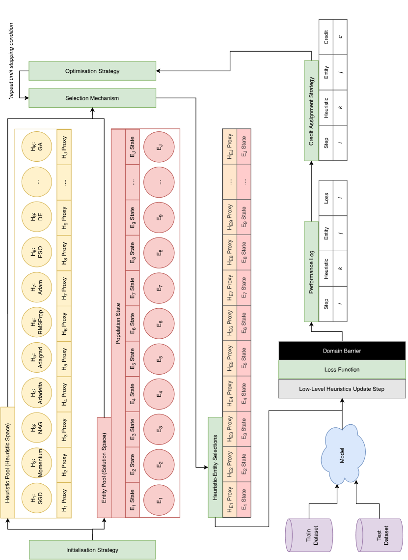
Figure 1: An illustration of the architecture and high level components of the BHH.

Algorithm 1 The pseudo-code for the implementation of the BHH

step $\leftarrow 0$

select initial heuristics

initialise population and entities

evaluate entities’ initial position

update population state

while stopping condition not met do

    for all entities in entity pool do

        if selected heuristic is gradient-based then

           get gradients

        end if

        apply low-level heuristic and proxy operations

        update population state

        log performance metrics to performance log

        if step ¡ burn-in window size then

           select heuristic

        else

           if step $\mathbin{\%}$ reanalysis interval = 0 then

               apply Bayesian analysis

           end if

           if step $\mathbin{\%}$ reselection interval = 0 then

               select heuristic

           end if

           if step $<$ replay window size then

               prune performance log

           end if

        end if

    end for

    step $\leftarrow$ step + $1$

end while

6.1 Heuristic Pool

Generally speaking, the heuristic pool is a collection of low-level heuristics under consideration by the BHH. The heuristic pool contains the set of low-level heuristics that, together with their performance information, make up the heuristic space. Importantly, the heuristic pool must consist of a diverse set of low-level heuristics with varying capabilities. This research takes an interest in including both gradient-based heuristics as well as MH in the heuristic pool. This approach is referred to as a multi-method approach.

6.2 Proxies

Heuristics often maintain a set of parameters that are used to control the behaviour of the heuristic. These parameters are refered to as heuristic state. The concept of proxies arises from the sparsity of state as maintained by different heuristics. Since heuristics maintain (possibly) different states, there is an uncertainty of state transition when switching between heuristics. A solution to state indifference is to proxy heuristic state update operations. State is then maintained in two parts: primary and proxied state. Primary state refers to the state that is originally maintained by a heuristic. Proxied state refers to the state that is not directly maintained by the heuristic, but can be updated by outsourcing the required state update operation to another heuristic. The BHH thus incorporates a mapping of proxied state update operations as given in the example in Table 1.

Table 1: An example of a mapping of proxied state update operation maintained by the BHH.

		State Parameter
		1	2	3
Heuristic	A	n/a	B	n/a
	B	n/a	n/a	A
	C	n/a	B	A

From the example given in Table 1, when heuristic A is selected, it will outsource state update operations from heuristic B for state parameter 2. Heuristic B will outsource from heuristic A for state parameter 3. Finally, heuristic C will outsource from heuristic A and B for state parameters 2 and 3 respectively. In this way, all heuristics maintain all the state parameters.

6.3 Entity Pool

The entity pool refers to a collection or population of entities that each represent a candidate solution to the underlying FFNN being trained. The BHH selects from the heuristic pool a low-level heuristic to be applied to an individual entity. The outcome of this selection process is a mapping table that tracks which heuristic has been selected for which entity. These heuristic-entity combinations are applied to the underlying FFNN. The BHH tracks the performance of each of these combinations throughout the training process in a performance log.

Entities represent candidate solutions to the model’s trainable parameters (weights) and other heuristic-specific state parameters. These state parameters are referred to as local state. Entities are treated as physical particles in a hyper-dimensional search environment. Entities model concepts from physics. For example, the candidate solution is represented as the entity’s position. The velocity and acceleration is then analogous to the gradient and momentum of the entity respectfully [32]. Examples of entity state parameters, as derived from various low-level heuristics, include entity position, velocity, gradient, position delta, first and second moments of the gradient, the loss, personal best positions, losses, and so on. The entity state parameters are updated by the associated heuristic.

The population state refers to a collection of parameters that are shared between the entities in the population. Population state is also referred to as global state and represents the population’s memory. The population state generally contains state parameters that are of importance to multiple heuristics, and usually tracks the state of the population and not individual heuristic. Some examples of population state that can arise from different heuristics include the population of entities themselves, the global best entity found so far, the overall best loss achieved thus far, and so on.

6.4 Performance Log

Heuristic selection probability is calculated based on heuristic-entity performance over time. Evidence of heuristic-entity performance is thus required for the BHH to learn. Historical heuristic-entity performance outcomes are stored in a performance log. The performance log tracks information such as the current step, selected heuristic, associated entity, the loss achieved and so on. Since the performance log can become very big, only a sliding window of the performance history is maintained at each step in the learning process. The sliding window is also referred to as a replay window/buffer.

6.5 Credit Assignment Strategy

The credit assignment strategy is a mechanism that assigns a discrete credit indicator to heuristics that perform well, based on their performance metrics such as loss. The credit assignment strategy implements a component of the “move acceptance” process as proposed by Özcan et al. [33] and addresses the credit assignment problem as discussed by Burke et al. [23]. A good credit assignment strategy will correctly allocate credit to the appropriate heuristic-entity combination. This research implements the following credit assignment strategies to choose from: ibest (iteration best), pbest (personal best), gbest (global best), rbest (replay window best), and symmetric, where credit is assigned to all entity-heuristic combinations, regardless of their performance.

6.6 Selection Mechanism

The BHH implements a probabilistic predictive model based on the fundamentals of the Naïve Bayes algorithm. The BHH thus distinguishes between the following events: $\boldsymbol{H}$, the event of observing heuristics, $\boldsymbol{E}$, the event of observing entities, and $\boldsymbol{C}$, the event of observing credit assignments that indicate that the credit assignment performance criteria are met. By Bayes’ theorem, the selection mechanism implemented by the BHH is given as

$$\begin{split}P(\boldsymbol{H}|\boldsymbol{E},\boldsymbol{C};\boldsymbol{\theta},\boldsymbol{\phi},\boldsymbol{\psi})&\propto P(\boldsymbol{E}|\boldsymbol{H};\boldsymbol{\phi})P(\boldsymbol{C}|\boldsymbol{H};\boldsymbol{\psi})P(\boldsymbol{H}|\boldsymbol{\theta})\end{split}$$ (1)

The predictive model thus models the proportional probability of the event (selection of) heuristic $\boldsymbol{H}$, given allocation to entity $\boldsymbol{E}$ and credit requirement $\boldsymbol{C}$, parameterised by sampled $\boldsymbol{\theta}\sim Dir(\boldsymbol{\alpha};K)$, $\boldsymbol{\phi}\sim Dir(\boldsymbol{\beta};K)^{J}$ and $\boldsymbol{\psi}\sim Beta(\gamma_{1},\gamma_{0})$. In the aforementioned, $K$ is the heuristic pool size and $J$ is the entity pool size. The parameters $\boldsymbol{\alpha}$, $\boldsymbol{\beta}$, $\gamma_{1}$ and $\gamma_{0}$ are referred to as concentration parameters. The concentration parameters are used to parameterise the prior probability distributions. A provides mathematical derivations of the predictive model.

6.7 Optimisation Step

The intent of the BHH is to gather evidence that can be used to update prior beliefs about which heuristics perform well during training. These beliefs are represented by the concentration parameters $\boldsymbol{\alpha}$, $\boldsymbol{\beta}$, $\gamma_{1}$ and $\gamma_{0}$. A change in prior beliefs is represented by a change in these concentration parameters. Specifically, it can be said that the optimisation process implemented by the BHH updates pseudo counts of events that are observed in the performance logs. These pseudo counts track the occurrence of a heuristic, an entity, and resulting performance of these two elements. Through the credit assignment strategy, these pseudo counts are biased towards entity-heuristic combinations that meet performance requirements and yield credit allocations.

Generally, there are two different techniques that are used to train Naïve Bayes classifiers. The frequentist approach implements MLE and the Bayesian approach implements MAP.

6.7.1 Maximum A Posteriori Estimation

MAP is an approach to optimise the values for $\hat{\theta}_{k}$, $\hat{\phi}_{j,k}$ and $\hat{\psi}_{k}$ by optimising the parameters of their probability distributions. This process is referred to as Bayesian analysis. Bayesian analysis makes use of the posterior probability distribution. The concentration update operations yielded by MAP, are given as follows:

$$\begin{split}\alpha_{k}(t+1)=N_{k}+\alpha_{k}(t)\end{split}$$ (2)

$$\begin{split}\beta_{j,k}(t+1)=N_{j,k}+\beta_{j,k}(t)\end{split}$$ (3)

$$\begin{split}\gamma_{1,k}(t+1)=N_{1,k}+\gamma_{1,k}(t)\end{split}$$ (4)

$$\begin{split}\gamma_{2,k}(t+1)=N_{0,k}+\gamma_{2,k}(t)\end{split}$$ (5)

where $N_{k}$ is a summary variable denoting the count of occurrences of heuristic $k$, $N_{j}$ is a summary variable denoting the count of occurrences of entity $j$, $N_{j,k}$ is a summary variable denoting the count of occurrences of heuristic $k$ for entity $j$, $N_{1,k}$ and $N_{0,k}$ are summary variables denoting the count of occurrences where heuristic $k$ meets performance requirements and where heuristic $k$ does not not meet performance requirements.

It can be said that the BHH implements a Gaussian process [34]. Since the reselection of heuristics happens at regular intervals, the outcome of a selection in one iteration may influence the outcome of another in the next iteration, making the implementation of the BHH a HMM [35].

6.8 Hyper-Parameters

The following hyper-parameters are implemented by the BHH: the heuristic pool configures the type of heuristics included in the heuristic pool, the population size specifies the number of entities in the entity pool, the credit assignment strategy specifies which credit assignment strategy to use, the reselection interval determines the frequency of heuristic reselection, the replay window size determines the maximum size of the performance log, the reanalysis interval determines the frequency at which Bayesian analysis is applied, the burn in window size determines the size of an initial window where experience is simply gathered without reanalysis, and finally, the discounted rewards and normalisation flags toggle scaling modifiers on values assigned by the credit assignment strategies, backwards in the performance log.

7 Methodology

This section provides the details of the implementation of the empirical process. At a high level the experimental procedure consist of a comparison between the BHH and standalone low-level heuristics. A number of datasets, models and heuristics are specified. Throughout the empirical process, a BHH baseline configuration is used.

7.1 BHH Baseline

The BHH baseline is a name given to a specific configuration of the BHH which has been found to provide a reasonable baseline performance. The baseline configuration is used as the cornerstone configuration from which all other heuristics and their configurations are evaluated. The BHH baseline configuration is given in Table 2. In Table 2, the heuristic pool configuration, all, refers to a configuration where the heuristic pool contains all the low-level heuristics, including all gradient-based heuristics and MH.

Table 2: The BHH baseline configuration as it is used in the empirical study.

heuristic pool	population	burn in	credit	reselection	replay	reanalysis	normalise	discounted rewards
all	5	0	ibest	10	10	10	false	false

7.2 BHH vs. Low-Level Heuristics

For the standalone heuristics experimental group, a number of low-level heuristics are used along with their specified hyper-parameters. Each of these standalone low-level heuristics is compared to that of the BHH baseline configuration, across all datasets. The intent of the standalone heuristics experimental group is to determine if the BHH baseline configuration can generalise to multiple problems in comparison to individual low-level heuristics.

Additional to the BHH baseline configuration, two more BHH configurations are included. These include BHH configurations where the heuristic pool only makes use of gradient-based heuristics, and a configuration where the heuristic pool only makes use of MH. The intent behind the inclusion of these configurations is to determine the effectiveness of multi-method approaches in the heuristic pool applied to training FFNN.

7.3 Heuristics

Table 3 contains a list of all the standalone, low-level heuristics that are used as well as their hyper-parameter configurations. In some cases, parameters are changed dynamically throughout the training process using a decay schedule. Note from Table 3 that values that are configured to make use of a decay schedule are presented with the initial value first and the decay rate in brackets next to it.

Table 3: Low-level heuristics and their hyper-parameter configurations.

heuristic	configuration	value	citation
sgd	learning rate	0.1 (0.01)	[12]
momentum	learning rate	0.1 (0.01)	[12]
	momentum	0.9
nag	learning rate	0.1 (0.01)	[12]
	momentum	0.9
adagrad	learning rate	0.1 (0.01)	[13]
	epsilon	1E-07
rmsprop	learning rate	0.1 (0.01)	[15]
	rho	0.95
	epsilon	1E-07
adadelta	learning rate	1.0 (0.95)	[14]
	rho	0.95
	epsilon	1E-07
adam	learning rate	0.1 (0.01)	[8]
	beta1	0.9
	beta2	0.999
	epsilon	1E-07
pso	population size	10	[36]
	learning rate	1.0 (0.9)
	inertia weight (w)	0.729844
	cognitive control (c1)	1.49618
	social control (c2)	1.49618
	velocity clip min	-1.0
	velocity clip max	1.0
de	population size	10	[37]
	selection strategy	best
	xo strategy	exp
	recombination probability	0.9 (0.1)
	beta	2.0 (0.1)
ga	population size	10	[38]
	selection strategy	rand
	xo strategy	bin
	mutation rate	0.2 (0.05)

The mapping of proxied heuristic state update operations implemented by the BHH in the empirical process is given in Figure 2. In Figure 2, cells containing x indicate that the associated heuristic implements that particular state parameter explicitly, and cells containing o indicate that the state parameter is implicitly implemented as part of the BHH algorithm.

Figure 2: Mapping of proxied heuristic state update operations as implemented by the BHH

7.4 Datasets

In the context of training FFNN, the underlying models are trained across a number of datasets. All the datasets used in the empirical process originate from the UCI Machine Learning Repository [39]. Datasets are grouped by problem type and include seven classification and seven regression datasets. The details around the datasets used can be found in Tables 4 and 5. Each dataset is split into a training set comprising 80% of the data, and a test set comprising 20% of the data.

A number of classification datasets contain an unbalanced representation of classes. This work does not apply mechanisms to cater for class balancing, in order to eliminate as many variables and factors in the empirical process as possible.

Table 4: Classification datasets

dataset	output	types	attributes	classes	instances	batch	steps	citation
iris	multivariate	real	4	3	150	16	10	[40]
car	multivariate	categorical	6	4	1728	128	14	[41]
abalone	multivariate	categorical, integer, real	8	28	4177	256	17	[42]
wine quality	multivariate	real	12	11	4898	256	20	[43]
mushroom	multivariate	categorical	22	2	8214	512	17	[44]
bank	multivariate	real	17	2	45211	512	89	[45]
diabetic	multivariate	integer	55	3	100000	1024	98	[46]

Table 5: Regression datasets

dataset	output	types	attributes	instances	batch	steps	citation
fish toxicity	multivariate	real	7	908	64	15	[47]
housing	univariate	real	13	506	32	16	[48]
forest fires	multivariate	real	13	517	32	17	[49]
student performance	multivariate	integer	33	649	32	21	[50]
parkinsons	multivariate	integer, real	26	5875	256	23	[51]
air quality	multivariate, time series	real	15	9358	256	37	[52]
bike	univariate	integer, real	16	17389	256	68	[53]

7.5 Models

All models trained in the empirical process follow implementations of shallow FFNN with only one hidden layer. The number of hidden units used were determined empirically. Weights are initialised by means of Glorot uniform sampling [54]. The models and their configuration, as it is used for each dataset, are given in Table 6.

Table 6: Model configurations

dataset	inputs	hidden	output	biases	parameters	topology	l1 activation	l2 activation
fish toxicity	6	3	1	yes	25	dense	LReLU ($\alpha=0.3$)	sigmoid
iris	4	5	3	yes	43	dense	LReLU ($\alpha=0.3$)	softmax
air quality	12	8	1	yes	113	dense	LReLU ($\alpha=0.3$)	sigmoid
housing	13	8	1	yes	121	dense	LReLU ($\alpha=0.3$)	sigmoid
wine quality	13	10	7	yes	217	dense	LReLU ($\alpha=0.3$)	softmax
parkinsons	21	10	1	yes	231	dense	LReLU ($\alpha=0.3$)	sigmoid
car	21	10	4	yes	264	dense	LReLU ($\alpha=0.3$)	softmax
forest fires	43	16	1	yes	721	dense	LReLU ($\alpha=0.3$)	sigmoid
abalone	10	36	28	yes	1432	dense	LReLU ($\alpha=0.3$)	softmax
bank	51	32	1	yes	1697	dense	LReLU ($\alpha=0.3$)	softmax
bike	61	32	1	yes	2017	dense	LReLU ($\alpha=0.3$)	sigmoid
student performance	99	32	1	yes	3233	dense	LReLU ($\alpha=0.3$)	sigmoid
adult	108	64	1	yes	7041	dense	LReLU ($\alpha=0.3$)	softmax
mushroom	117	64	1	yes	7617	dense	LReLU ($\alpha=0.3$)	softmax
diabetic	2369	32	3	yes	75939	dense	LReLU ($\alpha=0.3$)	softmax

7.6 Performance Measures

BinXE is used for classification problems with two classes and SparseCatXE is used for classification problems with more than two classes. For the classification problems, accuracy is also measured. For regression problems, the MSE is used as a performance metric. After training has completed, the average rank, based on test loss, for all configurations, is calculated at each mini-batch step.

7.7 Statistical Analysis

Each experiment and configuration is trained for a maximum of 30 epochs and is repeated over 30 independent runs, for each of the datasets. No early-stopping mechanism is used. Statistical analysis is executed on the results from the test datasets. An average rank is calculated across all 30 runs, for both experimental groups and configurations, at each step, for every epoch of training.

The Shapiro-Wilk test for normality [55] ($\alpha$ = 0.001) is used to determine if the results are normally distributed. The Levene’s test for equality of variance [56] ($\alpha$ = 0.001) is used. For experiments with three or more configurations, the ANOVA statistical test [57] ($\alpha$ = 0.001) is used. The Kruskal-Wallis ranked non-parametric test [58] for statistical significance ($\alpha$ = 0.001) is used for cases where data is not normally distributed. Finally, a post-hoc Tukey honest significant difference test [59] ($\alpha$ = 0.001) is used from which significant ranking is retrieved. Descriptive and critical difference plots are then retrieved from these results to provide visual aid.

7.8 Implementation

All implementations are done from first principles in Python 3.9 using Tensorflow 2.7 and Tensorflow Probability 0.15.0. The source code and data for this research is provided and made public at https://github.com/arneschreuder/masters.

8 Results

This section provides the results of the empirical process that has been conducted. Detailed discussions follow on the outcomes of each experiment.

8.1 Overview

This section provides a brief discussion on the general outcome of the empirical process as a whole and identifies some key aspects to be kept in mind when interpreting the results of the experiments.

Firstly, the BHH applies a form of online learning. As such, the BHH applies the learning mechanism during training in a single run of the training process. The training process is not repeated iteratively as is the case with some HH.

Most of the training progress is observed to occur within the first five epochs. As a result, the BHH should apply most learning at the early stages of the training process. After five epochs, the training of most of the underlying FFNN converges and little performance gain is observed after that point. Since this empirical process does not apply early stopping of the training process, the BHH will continue to explore the heuristic space beyond the five epoch mark.

The BHH does not implement a type of move-acceptance strategy where the application of a heuristic to an entity is only accepted if it leads to a better solution. In some cases, the BHH then selects heuristics that yield sub-optimal results, but is shown to mostly return to optimal solutions over a number of steps.

Given the stochastic nature of the heuristic selection mechanism, sufficient samples of the performance of each heuristics-entity combination in the performance log are required for the BHH to learn. This requirement is further strengthened by the Bayesian nature of the probabilistic model implemented by the BHH. The probabilistic model implements probability distributions of heuristic selection probabilities and as such, insufficient samples in the performance log could render a form of random search.

By default, the BHH baseline configuration has a reanalysis interval of 10, and a replay window size of 10, which is a small window to learn from. Despite the small reanalysis interval and the small replay window size, it should be observed that the BHH exploits small performance biases and finds small performance gains throughout.

8.2 BHH vs. Low-Level Heuristics

Tables 7 and 8 provide the empirical results in ranked format. The performance rank is calculated as the average rank produced by each heuristic, across all datasets, for all independent runs and all epochs. The average rank across all epochs produces a view on the performance of the heuristics as it relates to the entire training process. Finally, a normalised average rank is provided for the overall performance of all heuristics at the bottom of the table. The normalised average rank is calculated as a discrete normalisation of the average rank achieved across all datasets, for all independent runs and epochs.

Tables 7 and 8 show that the bhh_gd configuration produced the best results of the BHH variants and managed to perform well, producing generally good results across all datasets. The bhh_gd configuration managed to produce results that are comparable to the top three heuristics for each dataset, while the bhh_all and bhh_mh produced average results compared to all the heuristics.

Table 7: Empirical results showing normalised average rank and statistics for the top six low-level heuristics and three heuristic pool variants of the BHH baseline configuration, across multiple datasets, for all independent runs and epochs.

	BHH vs. Low-Level Heuristics - Average Rank (Part A)
dataset	adagrad	adam	rmsprop	bhh_gd	nag	bhh_all
abalone	2,2215 ($\pm$1,591)	2,3989 ($\pm$1,887)	4,6172 ($\pm$2,65)	4,7032 ($\pm$2,108)	4,2731 ($\pm$1,542)	5,9376 ($\pm$2,399)
air_quality	3,6409 ($\pm$2,259)	5,4312 ($\pm$2,62)	3,4452 ($\pm$2,57)	5,0817 ($\pm$2,762)	3,8194 ($\pm$2,229)	6,686 ($\pm$3,061)
bank	2,5495 ($\pm$1,598)	2,0796 ($\pm$1,587)	3,4645 ($\pm$2,209)	4,8828 ($\pm$1,702)	4,2871 ($\pm$1,732)	6,2419 ($\pm$2,157)
bike	1,7204 ($\pm$1,384)	3,6925 ($\pm$4,004)	6,2624 ($\pm$4,58)	3,8441 ($\pm$1,398)	6,4516 ($\pm$1,02)	4,2151 ($\pm$1,361)
car	4,7634 ($\pm$0,938)	1,6226 ($\pm$1,405)	2,3269 ($\pm$1,409)	3,3473 ($\pm$1,35)	6,0785 ($\pm$0,799)	3,5624 ($\pm$1,315)
diabetic	2,7796 ($\pm$1,659)	7,1484 ($\pm$2,227)	6,7376 ($\pm$2,577)	5,2269 ($\pm$2,186)	1,8118 ($\pm$1,413)	9,3968 ($\pm$3,022)
fish_toxicity	4,2645 ($\pm$2,614)	3,6022 ($\pm$2,445)	3,5946 ($\pm$2,329)	5,4118 ($\pm$2,665)	5,8914 ($\pm$2,629)	5,829 ($\pm$2,856)
forest_fires	5,1559 ($\pm$2,922)	4,2688 ($\pm$2,984)	5,0355 ($\pm$3,143)	4,6935 ($\pm$2,759)	5,6882 ($\pm$2,215)	5,4839 ($\pm$3,107)
housing	3,4484 ($\pm$2,025)	3,3344 ($\pm$1,819)	3,6946 ($\pm$2,166)	4,4742 ($\pm$2,312)	4,6839 ($\pm$2,658)	4,3763 ($\pm$2,438)
iris	6,3946 ($\pm$1,6)	3,5839 ($\pm$2,511)	2,6968 ($\pm$1,912)	4,7473 ($\pm$2,275)	3,5548 ($\pm$2,125)	5,2204 ($\pm$3,041)
mushroom	4,4656 ($\pm$1,053)	2,1344 ($\pm$1,883)	2,4656 ($\pm$1,359)	3,4484 ($\pm$1,602)	6,3323 ($\pm$0,891)	3,6688 ($\pm$2,469)
parkinsons	2,4677 ($\pm$1,497)	2,2333 ($\pm$1,742)	3,5656 ($\pm$2,492)	4,572 ($\pm$1,934)	7,5355 ($\pm$1,44)	4,3839 ($\pm$1,861)
student_performance	2,5634 ($\pm$1,912)	11,3978 ($\pm$2,178)	12,4312 ($\pm$1,34)	5,6624 ($\pm$3,57)	3,1935 ($\pm$2,12)	5,8634 ($\pm$3,159)
wine_quality	3,2806 ($\pm$1,931)	2,1118 ($\pm$1,666)	3,6301 ($\pm$1,731)	4,7882 ($\pm$2,105)	4,1505 ($\pm$1,916)	5,1925 ($\pm$1,951)
avg rank	3,5512 ($\pm$2,25)	3,9314 ($\pm$3,423)	4,5691 ($\pm$3,517)	4,6346 ($\pm$2,364)	4,8394 ($\pm$2,384)	5,4327 ($\pm$2,9)
normalised avg rank	1	2	3	4	5	6

Table 8: Empirical results showing normalised average rank and statistics for the bottom six low-level heuristics and three heuristic pool variants of the BHH baseline configuration, across multiple datasets, for all independent runs and epochs.

	BHH vs. Low-Level Heuristics - Average Rank (Part B)
dataset	adadelta	bhh_mh	ga	pso	sgd	momentum	de
abalone	5,3129 ($\pm$1,478)	8,1882 ($\pm$1,195)	11,1108 ($\pm$1,102)	11,2559 ($\pm$1,826)	8,628 ($\pm$1,019)	9,8151 ($\pm$1,16)	12,5376 ($\pm$1,329)
air_quality	5,2441 ($\pm$3,162)	6,357 ($\pm$2,303)	7,8204 ($\pm$2,265)	9,9151 ($\pm$2,288)	10,6613 ($\pm$1,606)	11,7559 ($\pm$1,473)	11,1419 ($\pm$2,236)
bank	5,672 ($\pm$1,241)	9,7495 ($\pm$1,048)	10,9817 ($\pm$1,216)	11,8376 ($\pm$1,464)	8,2774 ($\pm$1,03)	8,4774 ($\pm$1,068)	12,4989 ($\pm$1,224)
bike	5,3602 ($\pm$1,155)	7,4108 ($\pm$1,008)	9,2269 ($\pm$1,183)	9,3086 ($\pm$1,761)	10,3355 ($\pm$1,419)	10,7086 ($\pm$1,423)	12,4634 ($\pm$1,465)
car	7,7344 ($\pm$1,746)	8,8505 ($\pm$1,413)	10,7763 ($\pm$1,471)	8,3613 ($\pm$1,622)	10,2452 ($\pm$1,447)	10,9226 ($\pm$1,349)	12,4086 ($\pm$1,492)
diabetic	2,6753 ($\pm$1,629)	8,557 ($\pm$1,17)	11,2011 ($\pm$1,413)	10,7022 ($\pm$1,067)	5,9215 ($\pm$1,542)	6,3355 ($\pm$1,612)	12,5065 ($\pm$1,242)
fish_toxicity	7,914 ($\pm$3,429)	6,3849 ($\pm$2,944)	6,7043 ($\pm$2,82)	7,5731 ($\pm$2,982)	11,5785 ($\pm$1,459)	12,2301 ($\pm$1,382)	10,0215 ($\pm$2,358)
forest_fires	6,5161 ($\pm$3,082)	5,4591 ($\pm$2,668)	7,3667 ($\pm$2,37)	6,4796 ($\pm$3,354)	10,8129 ($\pm$1,207)	11,7065 ($\pm$1,325)	12,3333 ($\pm$1,923)
housing	7,5903 ($\pm$2,748)	7,5441 ($\pm$1,736)	7,8839 ($\pm$2,099)	9,9409 ($\pm$2,317)	11,4075 ($\pm$1,528)	11,2731 ($\pm$1,506)	11,3484 ($\pm$2,096)
iris	11,3527 ($\pm$1,779)	6,6075 ($\pm$2,555)	8,2473 ($\pm$1,765)	8,2731 ($\pm$4,384)	10,3796 ($\pm$1,294)	11,0548 ($\pm$1,409)	8,8871 ($\pm$3,251)
mushroom	6,5538 ($\pm$1,071)	9,0452 ($\pm$1,093)	11,5731 ($\pm$1,193)	7,872 ($\pm$0,92)	9,7527 ($\pm$1,083)	10,9785 ($\pm$1,108)	12,7097 ($\pm$1,478)
parkinsons	6,472 ($\pm$2,423)	8,3161 ($\pm$1,644)	7,7968 ($\pm$1,719)	8,4892 ($\pm$1,901)	11,7516 ($\pm$1,155)	12,5419 ($\pm$1,351)	10,8742 ($\pm$1,317)
student_performance	3,4194 ($\pm$2,006)	6,9333 ($\pm$2,44)	7,1032 ($\pm$1,989)	11,0624 ($\pm$1,067)	6,6366 ($\pm$2,023)	6,7011 ($\pm$2,242)	8,0323 ($\pm$1,935)
wine_quality	6,0011 ($\pm$2,404)	9,5935 ($\pm$1,494)	10,3387 ($\pm$1,62)	11,1602 ($\pm$1,773)	8,6344 ($\pm$1,18)	9,5269 ($\pm$1,341)	12,5903 ($\pm$1,352)
avg rank	6,2727 ($\pm$3,004)	7,7855 ($\pm$2,271)	9,1522 ($\pm$2,48)	9,4451 ($\pm$2,75)	9,6445 ($\pm$2,214)	10,2877 ($\pm$2,346)	11,4538 ($\pm$2,354)
normalised avg rank	7	8	9	10	11	12	13

The normalised average ranks provided in Tables 7 and 8 show that the bhh_gd configuration ranked fourth, while the bhh_al and bhh_mh configurations ranked sixth and eighth amongst all thirteen heuristic implementations respectively. These results show that the BHH generally performs well, but is not able to outperform the best heuristic for each dataset.

Figure 3 provides an illustration showing a descriptive plot of the average ranks achieved over all independent runs, for each heuristic, per dataset. The heuristics are ordered according to the normalised ranks presented in Tables 7 and 8. Figure 3 shows that the bhh_gd heuristic achieved the lowest variance in average rank across all datasets, compared to the other heuristics. The aforementioned shows the generalisation capabilities of the BHH to multiple problems.

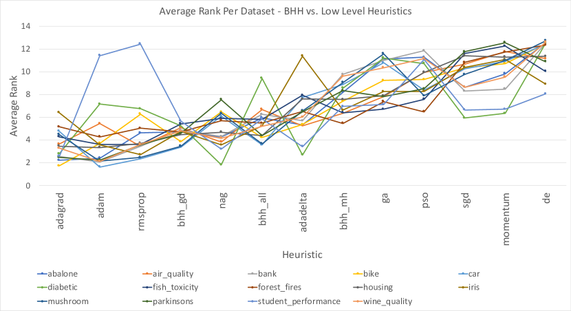
Figure 3: Descriptive plots for the average ranks of all low-level heuristics compared to three heuristic pool variants of the BHH baseline configuration, per dataset, across all independent runs and epochs.

Figure 4 provides an illustration of the overall critical difference plots that illustrate the statistically significant differences in ranked performance for each heuristic as it relates to all datasets, across all independent runs and epochs. Although the outcomes of the bhh_al and bhh_mh configurations seem to produce average performance results, it should be noted that the performance difference between all heuristics is very small. Furthermore, the best configuration of the BHH, namely the bhh_gd configuration, is statistically outperformed overall by only Adagrad and Adam, yielding statistically comparable results to RMSProp and NAG. It should be noted that the standalone low-level heuristics already produce good results in general across all datasets. In this particular case, producing better performance outcomes can be hard to achieve. However, as mentioned previously, the BHH provides a generalisation capability across all datasets that is advantageous to the BHH.

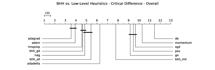
Figure 4: Critical difference plots for the average ranks of all low-level heuristics compared to three heuristic pool variants of the baseline BHH, across all datasets, runs and epochs.

Another observation that can be made is that the gradient-based heuristics generally performed much better than the MH on all datasets. State of the art methods for training FFNN, such as Adam, utilise gradient-based approaches that have been proven to work well on many occasions [8]. Exploration of the heuristic space leads the BHH to consider other heuristics during the training process, which could possibly result in worse performances at times. A suggestion to improve on these results is to include a move-acceptance strategy where heuristic progressions are discarded if they fail to produce better results.

9 Conclusion

The research done in this study stems from the difficult and tedious process of selecting the best heuristic for training FFNN. The research presented in this article identified the possibility of using a different approach, referred to as HH, to automate the heuristic selection process.

This research set out to develop a novel high-level heuristic that utilises probability theory in an online learning setting to drive the automatic heuristic selection process.

For the experimental group that compares the BHH baseline with a number of low-level heuristics, it was found that the bhh_gd configuration, which contains only gradient-based heuristics in the heuristic pool, performed the best out of the BHH variants, achieving an overall rank of fourth amongst thirteen heuristics that were implemented and executed on fourteen datasets. The bhh_gd configuration produced performance results close to that of the best low-level heuristics and was statistically outperformed only by the top two low-level heuristics. The bhh_all configuration, which contains only gradient-based heuristics and MH in the heuristic pool, achieved an overall rank of sixth, and the bhh_mh configuration, which contains only MH in the heuristic pool, achieved an overall rank of eighth.

Although the bhh_gd configuration produced performance results comparable to the best low-level heuristics, the bhh_all and bhh_mh configurations produced average results. It was found that, in general, gradient-based heuristics produced the best results, as such, it is understandable that the bhh_gd yielded the best performance outcomes between the different BHH variants that were implemented. Although the BHH variants were not able to produce better results than the top low-level heuristics, the BHH variants still effectively trained the underlying FFNN and produced good training outcomes overall. It was shown that the bhh_gd configuration produced the lowest variance in rank between datasets out of all of the heuristics implemented, giving the BHH the ability to generalise well to other problems.

Finally, it was shown that the BHH provides a mechanism whereby prior expert knowledge can be injected, before training starts. Future research can exploit this knowledge and provide a significant bias towards heuristics that are known to perform well on particular problem types. Future research can also investigate the scalability and effectiveness of the BHH on other model architectures such as DNN. Furthermore, the selection mechanism of the BHH can be extended to not just select heuristics from a heuristic pool, but also different model architectures from a model architecture pool.

Appendix A Naïve Bayes

This section aims to dissect the probabilistic model that is presented in Equation (1). The BHH implements a form of Naïve Bayes classifier, and thus independence between events can be assumed. The following derived PMF are provided as fundamental building blocks to show the mechanism by which the BHH learns.

The independence between events for class label $\boldsymbol{H}$, simply yields the PMF of the Multinomial distribution as presented below:

$$\begin{split}P(\boldsymbol{H}|\boldsymbol{\theta})&\propto\prod_{i=1}^{I}\prod_{k=1}^{K}P(h_{i,k}|\theta_{k})\\ &\propto\prod_{i=1}^{I}\prod_{k=1}^{K}\theta_{k}^{\mathbbm{1}_{1}(h_{i,k})}\\ &\propto\prod_{k=1}^{K}\theta_{k}^{\sum_{i=1}^{I}\mathbbm{1}_{1}(h_{i,k})}\\ &\propto\prod_{k=1}^{K}\theta_{k}^{N_{k}}\end{split}$$ (6)

where $N_{k}$ is a summary variable such that $N_{k}=\sum_{i=i}^{I}\mathbbm{1}_{1}(h_{i,k})$, denoting the count of occurrences of the event $h_{i}$ taking on class $k$ in $I$ independent, identical runs.

The independence between events $\boldsymbol{E}$, given class label $\boldsymbol{H}$, is denoted by the likelihood of $\boldsymbol{E}$, conditional to the occurrence of heuristic $k$ and model parameter $\boldsymbol{\phi}$ as follows:

$$\begin{split}P(\boldsymbol{E}|\boldsymbol{H};\boldsymbol{\phi})&\propto\prod_{i=1}^{I}\prod_{j=1}^{J}\prod_{k=1}^{K}P(e_{i,j,k}|h_{i,k};\phi_{j,k})\\ &\propto\prod_{i=1}^{I}\prod_{j=1}^{J}\prod_{k=1}^{K}\phi_{j,k}^{\mathbbm{1}_{1}(e_{i,j,k})\mathbbm{1}_{1}(h_{i,k})}\\ &\propto\prod_{j=1}^{J}\prod_{k=1}^{K}\phi_{j,k}^{\sum_{i}^{I}\left[\mathbbm{1}_{1}(e_{i,j,k})\mathbbm{1}_{1}(h_{i,k})\right]}\\ &\propto\prod_{j=1}^{J}\prod_{k=1}^{K}\phi_{j,k}^{N_{j,k}}\end{split}$$ (7)

where $N_{j,k}$ is a summary variable such that $N_{j,k}=\sum_{i=i}^{I}\mathbbm{1}_{1}(e_{i,j,k})\mathbbm{1}_{1}(h_{i,k})$, denoting the count of occurrences of the events $e_{i}$ taking on class $j$ and $h_{i}$ taking on class $k$, i.e. the count of occurrences of both entity $j$ and heuristic $k$ occurring together in $I$ independent, identical runs.

Finally, the independence between events for the performance criteria $\boldsymbol{C}$, given class label $\boldsymbol{H}$, is denoted by the likelihood of $\boldsymbol{C}$, conditional to the occurrence of heuristic $k$ and model parameter $\boldsymbol{\psi}$ as given below:

$$\begin{split}P(\boldsymbol{C}|\boldsymbol{H};\boldsymbol{\psi})&\propto\prod_{i=1}^{I}\prod_{k=1}^{K}P(c_{i,k}|h_{i,k};\psi_{k})\\ &\propto\prod_{i=1}^{I}\prod_{k=1}^{K}\psi_{k}^{\mathbbm{1}_{1}(c_{i,k})\mathbbm{1}_{1}(h_{i,k})}(1-\psi_{k})^{\mathbbm{1}_{0}(c_{i,k})\mathbbm{1}_{1}(h_{i,k})}\\ &\propto\prod_{k=1}^{K}\psi_{k}^{\sum_{i=1}^{I}\mathbbm{1}_{1}(c_{i,k})\mathbbm{1}_{1}(h_{i,k})}(1-\psi_{k})^{\sum_{i=1}^{I}\mathbbm{1}_{0}(c_{i,k})\mathbbm{1}_{1}(h_{i,k})}\\ &\propto\prod_{k=1}^{K}\psi_{k}^{N_{1,k}}(1-\psi_{k})^{N_{0,k}}\\ &\propto\prod_{k=1}^{K}\psi_{k}^{N_{1,k}}(1-\psi_{k})^{(N_{k}-N_{1,k})}\end{split}$$ (8)

where $N_{k}$ is the same summary variable as described for Equation (6). $N_{1,k}$ is a summary variable such that $N_{1,k}=\sum_{i=1}^{I}\mathbbm{1}_{1}(c_{i,k})\mathbbm{1}_{1}(h_{i,k})$, denoting the count of occurrences of the events $c_{i}$ taking on a success (i.e. $c_{i}=1$) and $h_{i}$ taking on class $k$, i.e. the count of occurrences of both succeeding in the performance criteria and heuristic $k$ occurring together in $I$ independent, identical runs. Similarly, $N_{0,k}=N_{k}-N_{1,k}$ denotes the count of occurrences of the events $c_{i}$ taking on a failure (i.e. $c_{i}=0$) and $h_{i}$ taking on class $k$.

Equations (6), (7) and (8) can be substituted into the proportional evaluation of the predictive model as given in Equation (1), resulting in

$$\begin{split}P(\boldsymbol{H}|\boldsymbol{E},\boldsymbol{C};\boldsymbol{\theta},\boldsymbol{\phi},\boldsymbol{\psi})&\propto P(\boldsymbol{E}|\boldsymbol{H};\boldsymbol{\phi})P(\boldsymbol{C}|\boldsymbol{H};\boldsymbol{\psi})P(\boldsymbol{H}|\boldsymbol{\theta})\\ &\propto\left[\prod_{j=1}^{J}\prod_{k=1}^{K}\phi_{j,k}^{N_{j,k}}\right]\left[\prod_{k=1}^{K}\psi_{k}^{N_{1,k}}(1-\psi_{k})^{(N_{k}-N_{1,k})}\right]\left[\prod_{k=1}^{K}\theta_{k}^{N_{k}}\right]\end{split}$$ (9)

Consider the practical implementation of the predictive model as shown in Equation (9). Computationally, the equation presented in Equation (9) will underflow on a real computer if the resulting probabilities are very small.

A.1 Numerical Stability

When Equation (9) is evaluated, the numerical stability is shown to underflow if the resulting probabilities from its parts are very small. Multiplication of multiple fractional parameters leads to an even smaller fractional number. Probabilities might be very low at some points during training. A solution to the aforementioned problem is to apply the log-sum-exp trick. The transformation of Equation (9) using the log-sum-exp trick is given as

$$\begin{split}LSE(P(h_{k}|e_{j},c_{1};\boldsymbol{\theta},\boldsymbol{\phi},\boldsymbol{\psi}))=\ln(\exp(\phi_{j,k})+\exp(\psi_{k})+\exp(\theta_{k}))\end{split}$$ (10)

References

- Rakitianskaia and Engelbrecht [2012] A. S. Rakitianskaia, A. P. Engelbrecht, Training feedforward neural networks with dynamic particle swarm optimisation, Swarm Intelligence 6 (2012) 233–270.
- Allen and Minton [1996] J. A. Allen, S. Minton, Selecting the right heuristic algorithm: Runtime performance predictors, in: Conference of the Canadian Society for Computational Studies of Intelligence, Springer, 1996, pp. 41–53.
- Burke et al. [2013] E. K. Burke, M. Gendreau, M. Hyde, G. Kendall, G. Ochoa, E. Özcan, R. Qu, Hyper-heuristics: A survey of the state of the art, Journal of the Operational Research Society 64 (2013) 1695–1724.
- Nel [2021] G. S. Nel, A hyperheuristic approach towards the training of artificial neural networks., Ph.D. thesis, University of Stellenbosch, 2021.
- Oliva and Martins [2019] D. Oliva, M. S. Martins, A bayesian based hyper-heuristic approach for global optimization, in: 2019 IEEE Congress on Evolutionary Computation (CEC), IEEE, 2019, pp. 1766–1773.
- Schmidhuber [2015] J. Schmidhuber, Deep learning in neural networks: An overview, Neural networks 61 (2015) 85–117.
- Zell [1994] A. Zell, Simulation neuronaler netze, volume 1, Addison-Wesley Bonn, 1994.
- Kingma and Ba [2014] D. Kingma, J. Ba, Adam: A method for stochastic optimization, International Conference on Learning Representations (2014).
- Engelbrecht [2007] A. Engelbrecht, Computational Intelligence: An Introduction, Wiley, 2007.
- Werbos [1994] P. J. Werbos, The roots of backpropagation: from ordered derivatives to neural networks and political forecasting, volume 1, John Wiley & Sons, 1994.
- Qian [1999] N. Qian, On the momentum term in gradient descent learning algorithms, Neural networks 12 (1999) 145–151.
- Sutskever et al. [2013] I. Sutskever, J. Martens, G. Dahl, G. Hinton, On the importance of initialization and momentum in deep learning, in: International conference on machine learning, PMLR, 2013, pp. 1139–1147.
- Duchi et al. [2011] J. Duchi, E. Hazan, Y. Singer, Adaptive subgradient methods for online learning and stochastic optimization., Journal of machine learning research 12 (2011).
- Zeiler [2012] M. D. Zeiler, Adadelta: an adaptive learning rate method, arXiv preprint arXiv:1212.5701 (2012).
- Hinton et al. [2012] G. Hinton, N. Srivastava, K. Swersky, Neural networks for machine learning lecture 6a overview of mini-batch gradient descent, Cited on 14 (2012) 2.
- Bengio [2000] Y. Bengio, Gradient-based optimization of hyperparameters, Neural computation 12 (2000) 1889–1900.
- Blum and Roli [2003] C. Blum, A. Roli, Metaheuristics in combinatorial optimization: Overview and conceptual comparison, ACM computing surveys (CSUR) 35 (2003) 268–308.
- Van Wyk [2014] A. B. Van Wyk, An Analysis of Overfitting in Particle Swarm Optimised Neural Networks, Master’s thesis, University of Pretoria, 2014.
- Gupta and Sexton [1999] J. N. Gupta, R. S. Sexton, Comparing backpropagation with a genetic algorithm for neural network training, Omega 27 (1999) 679–684.
- Shi and Eberhart [1998] Y. Shi, R. Eberhart, A modified particle swarm optimizer, in: 1998 IEEE international conference on evolutionary computation proceedings. IEEE world congress on computational intelligence (Cat. No. 98TH8360), IEEE, 1998, pp. 69–73.
- Price et al. [2006] K. Price, R. M. Storn, J. A. Lampinen, Differential evolution: a practical approach to global optimization, Springer Science & Business Media, 2006.
- Fraser [1957] A. S. Fraser, Simulation of genetic systems by automatic digital computers i. introduction, Australian journal of biological sciences 10 (1957) 484–491.
- Burke et al. [2010] E. K. Burke, M. Hyde, G. Kendall, G. Ochoa, E. Özcan, J. R. Woodward, A classification of hyper-heuristic approaches, in: Handbook of metaheuristics, Springer, 2010, pp. 449–468.
- Burke et al. [2003] E. Burke, G. Kendall, J. Newall, E. Hart, P. Ross, S. Schulenburg, Hyper-heuristics: An emerging direction in modern search technology, in: Handbook of metaheuristics, Springer, 2003, pp. 457–474.
- Dowsland et al. [2007] K. A. Dowsland, E. Soubeiga, E. Burke, A simulated annealing based hyperheuristic for determining shipper sizes for storage and transportation, European Journal of Operational Research 179 (2007) 759–774.
- Grobler et al. [2012] J. Grobler, A. P. Engelbrecht, G. Kendall, V. Yadavalli, Investigating the use of local search for improving meta-hyper-heuristic performance, in: Evolutionary Computation (CEC), 2012 IEEE Congress on, IEEE, 2012, pp. 1–8.
- Van der Stockt and Engelbrecht [2018] S. A. Van der Stockt, A. P. Engelbrecht, Analysis of selection hyper-heuristics for population-based metaheuristics in real-valued dynamic optimization, Swarm and Evolutionary Computation (2018).
- Vrugt and Robinson [2007] J. A. Vrugt, B. A. Robinson, Improved evolutionary optimization from genetically adaptive multimethod search, Proceedings of the National Academy of Sciences 104 (2007) 708–711.
- Bayes [1763] T. Bayes, Lii. an essay towards solving a problem in the doctrine of chances. by the late rev. mr. bayes, frs communicated by mr. price, in a letter to john canton, amfr s, Philosophical transactions of the Royal Society of London (1763) 370–418.
- Hackenberger [2019] B. K. Hackenberger, Bayes or not bayes, is this the question?, Croatian medical journal 60 (2019) 50.
- Wackerly et al. [2014] D. Wackerly, W. Mendenhall, R. L. Scheaffer, Mathematical statistics with applications, Cengage Learning, 2014.
- Eberhart and Kennedy [1995] R. Eberhart, J. Kennedy, Particle swarm optimization, in: Proceedings of the IEEE international conference on neural networks, volume 4, Citeseer, 1995, pp. 1942–1948.
- Özcan et al. [2006] E. Özcan, B. Bilgin, E. E. Korkmaz, Hill climbers and mutational heuristics in hyperheuristics, in: Parallel Problem Solving from Nature-PPSN IX, Springer, 2006, pp. 202–211.
- Görtler et al. [2019] J. Görtler, R. Kehlbeck, O. Deussen, A visual exploration of gaussian processes, Distill 4 (2019) e17.
- Rabiner and Juang [1986] L. Rabiner, B. Juang, An introduction to hidden markov models, ieee assp magazine 3 (1986) 4–16.
- Van den Bergh and Engelbrecht [2010] F. Van den Bergh, A. P. Engelbrecht, A convergence proof for the particle swarm optimiser, Fundamenta Informaticae 105 (2010) 341–374.
- Mezura-Montes et al. [2006] E. Mezura-Montes, J. Velázquez-Reyes, C. A. Coello Coello, A comparative study of differential evolution variants for global optimization, in: Proceedings of the 8th annual conference on Genetic and evolutionary computation, 2006, pp. 485–492.
- Lambora et al. [2019] A. Lambora, K. Gupta, K. Chopra, Genetic algorithm - a literature review, in: 2019 International Conference on Machine Learning, Big Data, Cloud and Parallel Computing (COMITCon), 2019, pp. 380–384.
- Dua and Graff [2017] D. Dua, C. Graff, Uci machine learning repository, 2017. URL: http://archive.ics.uci.edu/ml.
- Fisher [1936] R. A. Fisher, The use of multiple measurements in taxonomic problems, Annals of eugenics 7 (1936) 179–188.
- Bohanec and Rajkovic [1988] M. Bohanec, V. Rajkovic, Knowledge acquisition and explanation for multi-attribute decision making, in: 8th Intl Workshop on Expert Systems and their Applications, Citeseer, 1988, pp. 59–78.
- Waugh [1995] S. G. Waugh, Extending and benchmarking Cascade-Correlation: extensions to the Cascade-Correlation architecture and benchmarking of feed-forward supervised artificial neural networks, Ph.D. thesis, University of Tasmania, 1995.
- Cortez et al. [2009] P. Cortez, A. Cerdeira, F. Almeida, T. Matos, J. Reis, Modeling wine preferences by data mining from physicochemical properties, Decision support systems 47 (2009) 547–553.
- Schlimmer [1987] J. C. Schlimmer, Concept acquisition through representational adjustment, Ph.D. thesis, University of California, Irvine, 1987.
- Moro et al. [2014] S. Moro, P. Cortez, P. Rita, A data-driven approach to predict the success of bank telemarketing, Decision Support Systems 62 (2014) 22–31.
- Strack et al. [2014] B. Strack, J. P. DeShazo, C. Gennings, J. L. Olmo, S. Ventura, K. J. Cios, J. N. Clore, Impact of hba1c measurement on hospital readmission rates: analysis of 70,000 clinical database patient records, BioMed research international 2014 (2014).
- Cassotti et al. [2015] M. Cassotti, D. Ballabio, R. Todeschini, V. Consonni, A similarity-based qsar model for predicting acute toxicity towards the fathead minnow (pimephales promelas), SAR and QSAR in Environmental Research 26 (2015) 217–243.
- Harrison Jr and Rubinfeld [1978] D. Harrison Jr, D. L. Rubinfeld, Hedonic housing prices and the demand for clean air, Journal of environmental economics and management 5 (1978) 81–102.
- Cortez and Morais [2007] P. Cortez, A. Morais, A data mining approach to predict forest fires using meteorological data, New Trends in Artificial Intelligence, Proceedings of the 13th EPIA, APPIA, Guimarães, Portugal, 2007, pp. 512–523.
- Cortez and Silva [2008] P. Cortez, A. M. G. Silva, Using data mining to predict secondary school student performance, Proceedings of 5th Future Business Technology Conference (FUBUTEC), EUROSIS-ETI, 2008, pp. 5–12.
- Tsanas et al. [2009] A. Tsanas, M. Little, P. McSharry, L. Ramig, Accurate telemonitoring of parkinson’s disease progression by non-invasive speech tests, Nature Precedings (2009) 1–1.
- De Vito et al. [2008] S. De Vito, E. Massera, M. Piga, L. Martinotto, G. Di Francia, On field calibration of an electronic nose for benzene estimation in an urban pollution monitoring scenario, Sensors and Actuators B: Chemical 129 (2008) 750–757.
- Fanaee-T and Gama [2014] H. Fanaee-T, J. Gama, Event labeling combining ensemble detectors and background knowledge, Progress in Artificial Intelligence 2 (2014) 113–127.
- Glorot and Bengio [2010] X. Glorot, Y. Bengio, Understanding the difficulty of training deep feedforward neural networks, in: Proceedings of the thirteenth international conference on artificial intelligence and statistics, 2010, pp. 249–256.
- Shapiro and Wilk [1965] S. S. Shapiro, M. B. Wilk, An analysis of variance test for normality (complete samples), Biometrika 52 (1965) 591–611.
- Levene [1961] H. Levene, Robust tests for equality of variances, Contributions to probability and statistics. Essays in honor of Harold Hotelling (1961) 279–292.
- Fisher et al. [1921] R. A. Fisher, et al., 014: On the “probable error” of a coefficient of correlation deduced from a small sample, Metron (1921) 3–32.
- Kruskal and Wallis [1952] W. H. Kruskal, W. A. Wallis, Use of ranks in one-criterion variance analysis, Journal of the American statistical Association 47 (1952) 583–621.
- Tukey [1949] J. W. Tukey, Comparing individual means in the analysis of variance, Biometrics (1949) 99–114.