Multidimensional Joint Recurrence Quantification Analysis:
detecting coupling between time series of different dimensionalities

Abstract

One issue with the analysis of complex systems and the interaction between such systems is that they are composed of different number of components, or simply the fact that a different number of observables is available for each system. The challenge is how to analyze the interaction of two systems which are not described by the same number of variables. The approach is to combine different types and number of time series so that they yield a matched set of data points from which coupling or correlation properties can be estimated. Here, we present multidimensional joint recurrence quantification analysis (MdJRQA), a recurrence-based technique that allows to analyze coupling properties between multivariate data sets that differ in dimensionality (i.e., number of observables) and type of data (such as nominal or interval-scaled, for example). First, we introduce the methods, and then test it on simulated data from linear and nonlinear systems. Finally, we discuss practical issue regarding the application of the method.

Sebastian Wallot0000-0002-3626-3940 Dan Mønster0000-0001-9639-8823 Correspondence concerning this article should be addressed to E-mail: danm@econ.au.dk

1 Introduction

The current paper presents an extension of extant recurrence analysis techniques, joint recurrence quantification analysis (JRQA; [15]) and multidimensional recurrence quantification analysis (MdRQA; [33]), that is particularly aimed at quantifying the correlation—or coupling—between time series that differ in dimensionality. That is, assessing coupling between two systems with different number of observed variables. Examples include correlating a high-dimensional neurophysiological recording (e.g., electroencephalogram, functional magnetic resonance imaging, etc.) with a unidimensional behavior stream (e.g., gaze fixation times), or the behavior of a group leader (e.g., unidimensional acceleration profile or transcript of speech) with the collective behavior of the other group members (e.g., multidimensional acceleration profile or transcript of speech, where each group member adds one or more variables to the multivariate group dynamics).

The advantage of the proposed method is that multidimensional signals do not need to be averaged in order to reduce their dimensionality to one [17], or to the dimension of a lower-dimensional time series that they are to be correlated with — as it is a general requirement of correlational methods to have matched set of paired data points in order to estimate correlation. In the approach we are presenting here, the full dynamics of the multivariate time series are retained for analysis in terms of their recurrence profile.

This can have particular advantages if the (multidimensional) time series in question exhibit complicated dynamics ([8]; [23]; [21]; [4]), exhibit autocorrelation in terms of fractal fluctuations (a.k.a., long-memory, $1/f$ noise) ([25]; [12];[11]; [9]), or inter-dependencies in terms of fractal correlations ([1]; [14]). Particularly the occurrence of multifractal fluctuations in human behavioral and neurophysiological data suggests that different time series measured from a single organism show such interdependencies ([6]; [10]). In all of these cases, fluctuations are informative about the behavior of the system, and would get lost by averaging of the signals.

Some of the current alternatives are various bi-variate analyses (Cross-Correlation, [19]; Cross-Recurrence, [24]; relative phase analysis, [2]; convergent-cross mapping, [26]; and many others), which can also be arranged to provide a network-analytic portrait (e.g., [20]). However, such analyses only capture bi-variate relationships among the individual observables, but do not capture higher-level dynamics. Another approach is to reduce the dimensionality of the data, for example by simply averaging across all component time series. This, however, leads to problems of how to normalize or weight these individual time series, and runs a high risk of averaging out interesting dynamics from the data. The same goes for other techniques of dimension reduction, such as principal component analysis or fractal analysis — which have the additional problem that the estimates of techniques are potentially vulnerable to auto-correlation properties that are usually present in time series data [29]. Finally, there are correlation methods that provide averages on the level or correlation parameters, such as canonical correlation [28] or multidimensional cross-recurrence quantification analysis [30]. While they are multivariate analyses that take inter-correlations among the different observables of multivariate time series into account, they always need a matching number of data points and variables. As we will see, the method we propose here, MdJRQA, contains such analyses as a special case, but generalizes to situations where we seek to quantify correlation between two multivariate time series that do not have a matched number of observables. Moreover, MdJRQA keeps the dynamics of the time series, and does not lose information inherent in fluctuations that are otherwise lost the in averaging process [31].

The present article is structured as follows: First, we provide a formal description of MdJRQA. Then, we will test the methods on example data from a non-linear, as well as a linear system.

1.1 Multidimensional Joint Recurrence Quantification Analysis (MdJRQA)

Multidimensional Joint Recurrence Quantification Analysis (MdJRQA) extends Multidimensional Recurrence Quantification Analysis [[, MdRQA;]]wallot_multidimensional_2016 by combining it with Joint Recurrence Plots [[, JRPs;]]romano_multivariate_2004, a method to extract measures of similarity between two time series. The idea behind MdJRQA is that if two systems—or two subsystems of a larger system—are coupled to each other, then this coupling will affect the dynamics of the systems in ways that can be quantified by looking at simultaneous recurrences (i.e., joint recurrences) of the two systems. In this section, we will briefly explain MdRQA and JRP as well as how we combine these methods to obtain MdJRQA. A conceptual overview of the method is provided in Fig. 1 for an example where a 3-dimensional system is coupled to a 2-dimensional system (explained in more detail in the section ‘Model system I’).

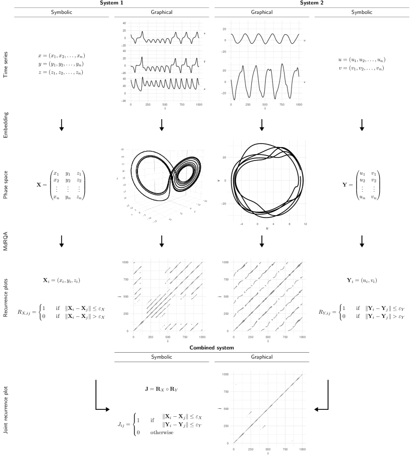
Figure 1: Conceptual overview of constructing a multidimensional joint recurrence plot. Two systems with respectively 3 and 2 scalar times series are embedded into a higher dimensional space. Here, the simplest example where the phase spaces have 3 and 2 dimensions is used for simplicity. The rows in $\mathbf{X}$ and $\mathbf{Y}$ represent points in phase space. Individual recurrence plots are constructed and combined into a joint recurrence plot.

For the purpose of our brief explanation in this section, we assume that we are dealing with a time series, i.e., a set of measurements at regular intervals of time of a single variable $x$ to give a set of values $(x_{1},x_{2},\ldots,x_{n})$. We further assume that $x$ is one of several variables needed to fully describe some system, and that an approximate description of the full system can be obtained by the method of time-delayed embedding [27], resulting in the construction of a multidimensional phase space embedding of the uni-dimensional variable $x$. If $x$ is embedded into an $m$-dimensional space with time delay $\tau$ the points will be vectors of the form

$$\mathbf{X_{i}}=(x_{i},x_{i-\tau},x_{i-2\tau},\ldots,x_{i-(m-1)\tau}).$$ (1)

The embedding parameters $m$ and $\tau$ are not given a priori, but must be estimated from the data [32].

The fundamental concept of all recurrence-based methods is the recurrence plot [7] which is a graphical visualization of when a system’s state recurs, i.e., if the system is in a state $\mathbf{X}_{1}=(X_{1},X_{2},\ldots,X_{m})$ at time $t_{1}$ and again at time $t_{2}$, the points $(t_{1},t_{2})$ and $(t_{2},t_{1})$ will be included in the recurrence plot of $x$. We can formulate this mathematically in terms of the recurrence matrix $\mathbf{R}$ with elements

$$R_{ij}=\begin{cases}1&\quad\text{if}\quad\|\mathbf{X}_{i}-\mathbf{X}_{j}\|\leq\varepsilon\\ 0&\quad\text{if}\quad\|\mathbf{X}_{i}-\mathbf{X}_{j}\|>\varepsilon.\end{cases}$$ (2)

Here, $\|\cdot\|$ is a norm in the $m$-dimensional phase space (usually the Euclidean distance) and $\varepsilon$ is a small radius within which two points will be considered equal and therefore recurrent (see [15] for a comprehensive introduction to recurrence plots).

A joint recurrence plot (JRP) is an element-wise product of two separate recurrence plots (recurrence matrices) with the same dimensions. This means that a JRP has elements with value 1 when both of the individual RP’s have the value 1 for a particular pair of times $(t_{1},t_{2})$. If we have the time series $x$ and another time series $y$ with phase space coordinates $\mathbf{X}_{i}$ and $\mathbf{Y}_{i}$ (constructed according to Eq. 1) then we can define the joint recurrence matrix $\mathbf{J}$ by its elements

$$J_{ij}=\begin{cases}1&\quad\text{if}\quad\|\mathbf{X}_{i}-\mathbf{X}_{j}\|\leq\varepsilon_{x}\quad\text{and}\quad\|\mathbf{Y}_{i}-\mathbf{Y}_{j}\|\leq\varepsilon_{y}\\ 0&\quad\text{otherwise}.\end{cases}$$ (3)

Here $\varepsilon_{x}$ and $\varepsilon_{y}$ are the radius parameters defining recurrences of $x$ and $y$, respectively. If $x$ has the recurrence matrix $\mathbf{R}_{x}$ and $y$ has the recurrence matrix $\mathbf{R}_{y}$ then the above can also be written $\mathbf{J}=\mathbf{R}_{x}\circ\mathbf{R}_{y}$, where “$\circ$” denotes the element-wise product of two matrices.

Multidimensional Recurrence Quantification Analysis [[, MdRQA;]]wallot_multidimensional_2016 is an extension of Recurrence Quantification Analysis [[, RQA;]]webber_dynamical_1994 where an inherently multidimensional time series can be analyzed. It also allows multiple uni-dimensional time series—such as data from a group of interacting individuals—to be aggregated into a multidimensional time series, thus facilitating the analysis of data from groups larger than dyads. So, while RQA quantifies the dynamics of a univariate time series, MdRQA quantifies the dynamics of a multivariate time series which may be constructed from several univariate time series considered to be parts of a bigger dynamical system. It can be viewed as a generalized time-dependent multivariate correlation measure, which along with the relevant multidimensional parameter estimation methods [32] are readily available through the R package ‘crqa’ [3].

We now combine JRP and MdRQA to construct the method of Multidimensional Joint Recurrence Quantification Analysis (MdJRQA). The method is applicable to situations where there are two interacting systems or sub-systems, where one or both are best described using a multivariate time series. In essence, the method is to first use the techniques of MdRQA to construct a recurrence plot (i.e., a recurrence matrix) for each of the two systems based on the multivariate time series. The multidimensional joint recurrence plot is then constructed as the element-wise product of the recurrence matrices for the two systems.

2 Methods

2.1 Model system I: The Three-dimensional Lorenz system and a two-dimensional harmonic oscillator

To determine how well MdJRQA recurrence is able to detect coupling between two systems when nonlinear, time-dependent dynamics are involved, we construct a model system, where all the interactions are known and can be varied. We have chosen a system consisting of two coupled sub-systems; the Lorenz system and a harmonic oscillator. The Lorenz system is characterized by chaotic behavior, a strange attractor and sensitive dependence on initial conditions. It was introduced by Lorenz as a simplified model for convection in the atmosphere [13]. The harmonic oscillator describes the dynamics of a system under a force that is proportional to the displacement from the static equilibrium state. This can describe, e.g., a mass on a spring, a pendulum with small amplitude motion and certain electrical circuits. The harmonic oscillator displays predictable periodic dynamics, and the attractor is a circle or ellipse. The combined model is illustrated graphically in Fig. 2, and described mathematically in the following.

Figure 2: Illustration of interaction between variables in the model consisting of the Lorenz system and the harmonic oscillator, described by Eq. 2.1. The variables $x,y,z,u,v$ are shown as solid circles, and terms linking one variable, e.g., $x$ to another, e.g., $y$ is shown as an arrow. For example the arrow from $x$ to $y$ with the label $\rho$ indicates a term of the form $\rho x$ in the expression for $\dot{y}$ in Eq. 2.1. Combinations of variables are shown as dashed circles, e.g., the term $xz$. By summing over all incoming arrows, we get the full expression: $\dot{y}=\rho x-xz-y$. The final term comes from the arrow from $y$ looping back to $y$ and since there is a factor $-1$ on the arrow it has a negative sign.

The Lorenz system is described by coupled first-order differential equations for the three variables $x$, $y$, and $z$

$$\dot{x} =\frac{\mathrm{d}x}{\mathrm{d}t}=\sigma\left(y-x\right)$$

$$\dot{y} =\frac{\mathrm{d}y}{\mathrm{d}t}=x\left(\rho-z\right)-y$$ (4)

$$\dot{z} =\frac{\mathrm{d}z}{\mathrm{d}t}=xy-\beta z$$

where $\dot{x}$ is the derivative of $x$ with respect to time and $\sigma$, $\rho$, and $\beta$ are parameters in the model, which have the canonical values $\sigma=10$, $\rho=28$, and $\beta=8/3$. The numerical solution to the three coupled differential equations in Eq. 2.1 gives rise to the famous Lorenz butterfly attractor (the phase space plot of system 1 in Fig. 1).

The harmonic oscillator is described by the second order differential equation

$$\ddot{u}=\frac{\mathrm{d}^{2}u}{\mathrm{d}t^{2}}=-ku,$$ (5)

for the variable $u$, where $k$ is a constant determining how big the force resulting from the displacement $u$ is. By introducing the velocity $v=\dot{u}$ the above second order differential equation can be written as two coupled first order differential equations, which exhibits the two-dimensional nature of the harmonic oscillator system:

$$\dot{u} =v\qquad{} \dot{v} =-ku$$ (6)

The combined model system is composed of the Lorenz system and and harmonic oscillator system with a coupling term (force) proportional to $x^{2}$ that perturbs the harmonic oscillator:

$$\dot{x} =\sigma\left(y-x\right)\quad{} \dot{u} =v$$

$$\dot{y} =x\left(\rho-z\right)-y\quad{} \dot{v} =-ku+cx^{2}$$ (7)

$$\dot{z} =xy-\beta z{}$$

These are the equations from Eq. 2.1 and 6 with the addition of the term $cx^{2}$ that is a unidirectional coupling from the Lorenz system to the harmonic oscillator system. We refer to $c$ as the coupling constant or coupling strength. In the limit of $c=0$ we recover two separate, uncoupled, systems. The connections between the variables in the two coupled systems described by Eq. 2.1 are illustrated in Fig. 2.

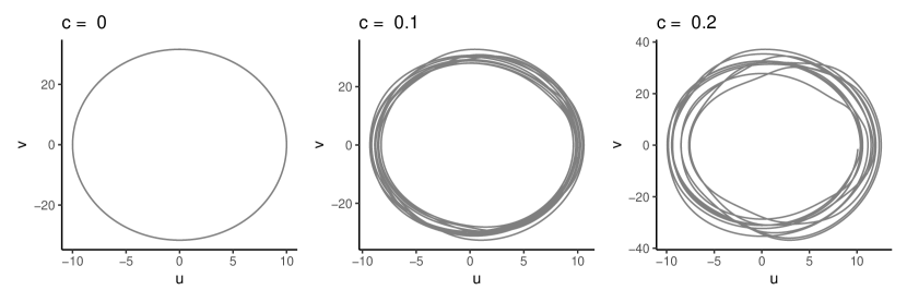
Figure 3: The phase space trajectory of the harmonic oscillator for different values of the coupling strength, $c$. For $c=0$ the attractor is an ellipse, and with increasing values of $c$ the attractor becomes increasingly irregular as the harmonic oscillator is perturbed by the Lorenz system.

Figure 3 illustrates the change in the dynamics of the harmonic oscillator for different coupling strengths $c$. For zero coupling $(c=0)$ the attractor is that of the isolated harmonic oscillator, viz., an ellipse, whereas, for nonzero coupling, the influence from the Lorenz system becomes more and more evident. It is this increasing influence that leads to an increase in joint recurrences between the two subsystems. Fig. 4 shows the result of the multidimensional joint recurrence quantification analysis when the coupled Lorenz system and the harmonic oscillator are investigated for different values of $c$. As can be seen, joint recurrence increases with increasing coupling strength $c$, capturing the effects of $c$ on the similarity of the dynamics of the two systems. In order to produce the plot in Fig. 4 it is important to keep the recurrence rate of the individual subsystems fixed, since otherwise a change in subsystem recurrence rate could be driving the change in joint recurrences. Here we display only the relative recurrence rate, i.e., the recurrence rate relative to the value at zero coupling. While the individual subsystem recurrence is kept fixed, the relative joint recurrence rate increases monotonically with $c$. What is not evident from Fig. 4 is that the joint recurrence rate is much lower than the subsystem recurrence rate. However this can be seen in the recurrence plots in Fig. 1 and will be elaborated on in the next section.

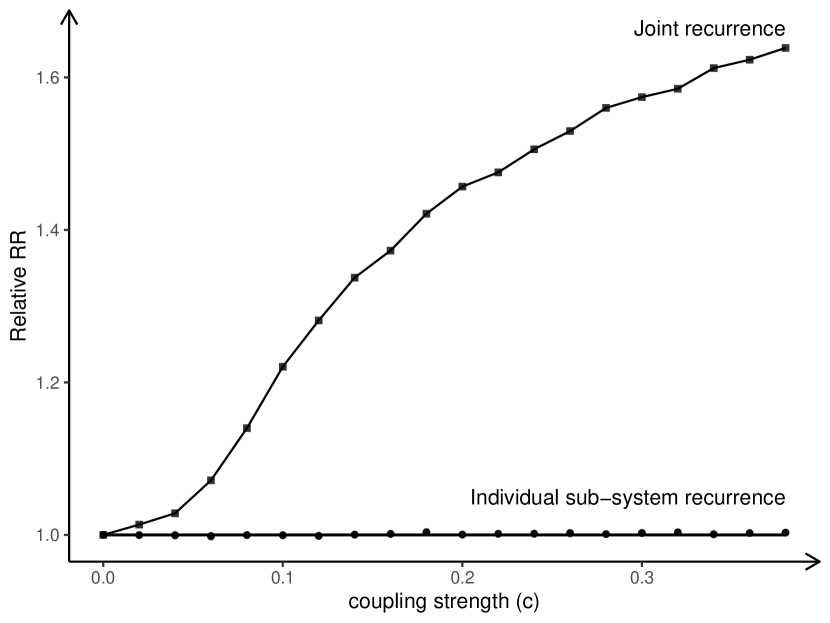
Figure 4: The relative recurrence rate, i.e., the recurrence rate divided by the recurrence rate at vanishing coupling strength ($c=0$). For the two comprising subsystems, the relative recurrence rates ($\bullet$) are fixed at values very close to $1$ (the horizontal line). For the multidimensional joint recurrence ($\blacksquare$), the relative recurrence rate increases monotonically with the coupling strength $c$.

2.2 Model system II: Two-dimensional and a one dimensional random process

To determine how well MdJRQA is able to detect correlations between a two-dimensional and a one dimensional random process, we conducted a simple simulation where one system, reflected by one random variable, $x_{1}$ is composed of a single source of variation, $\varepsilon_{1}$. The other system is reflected by two random variables, $y_{1}$ and $y_{2}$. Each of these variables is composed of two sources of variation, one that provides idiosyncratic variability to each of the two variables, $\varepsilon_{2}$ and $\varepsilon_{3}$, respectively, and another random variables, $\varepsilon_{4}$, which provides a common source of variability to both variables, highlighting that $y_{1}$ and $y_{2}$ both belong to one systems that introduces shared dynamics. To introduce coupling between the two systems, we use a weight $\beta_{1}$, which we varied between 0 (no correlation) and 10 (strong correlation) to change the correlation strength between the one dimensional time series $x_{1}$ and the two-dimensional time series $y_{1}$ and $y_{2}$. The variables are defined as follows (see also Fig. 5):

$$x_{1} =\varepsilon_{1}$$

$$y_{1} =\beta_{1}x_{1}+\varepsilon_{2}+\varepsilon_{4}$$ (8)

$$y_{2} =\beta_{1}x_{1}+\varepsilon_{3}+\varepsilon_{4}$$

Here $\beta_{1}\in[0,10]$, and

$$\begin{array}[]{cc}\varepsilon_{1}\sim N(0,1)&\varepsilon_{2}\sim N(0,1)\\ \varepsilon_{3}\sim N(0,1)&\varepsilon_{4}\sim N(0,1)\end{array}$$ (9)

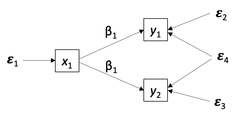
Figure 5: Illustration of composition of the two and one dimensional random variables described by Eq. 2.2.

Because the data are random variables, no embedding is needed. Hence the embedding dimension and the delay parameter are set to 1. The threshold parameter for computing the unidimensional recurrence plot of $x_{1}$ was set to a value to yield approximately 10 percent recurrence rate for each plot, and the threshold parameter for the multidimensional recurrence plot of $y_{1}$ and $y_{2}$ was likewise set to a value that yielded about the same percentage of recurrence points for each plot. This is done in order to give none of the two RPs priority over each other (see section Multidimensional Joint Recurrence Quantification Analysis (MdJRQA), above).

Using these settings, we varied the coupling parameter $\beta_{1}$ from 0 to 10 in step sizes of 0.5, and ran 100 instantiations of the random variables for each value of $\beta_{1}$. Each time series, $x_{1}$, $y_{1}$, and $y_{2}$, had a length of N = 100 data points. The results are shown in Fig. 7. Just as in Fig. 6, we see that relative joint recurrence rate increases with $\beta_{1}$.

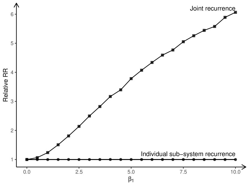
Figure 6: The relative recurrence rate, i.e., the recurrence rate divided by the recurrence rate at vanishing coupling strength ($\beta_{1}=0$). For the two comprising subsystems, the relative recurrence rates ($\bullet$) are fixed at values very close to $1$ (the horizontal line). For the multidimensional joint recurrence ($\blacksquare$), the relative recurrence rate increases monotonically with the coupling strength $\beta_{1}$.

Fig. 7 presents the raw values for average percentage recurrence of the individual RPs, as well as for the joint RP. Here, the upper panel shows the average level of sub-system recurrence for each value of $\beta_{1}$, which is about 10 percent. The lower panel shows the average level of joint recurrence between the two systems as a function of $beta_{1}$. As can be seen, recurrence increases with increasing values of $\beta_{1}$. Moreover, we also notice that for no coupling (i.e., $\beta_{1}=0$), we do not get 0 percent recurrence, but rather about 1 percent of recurrence.

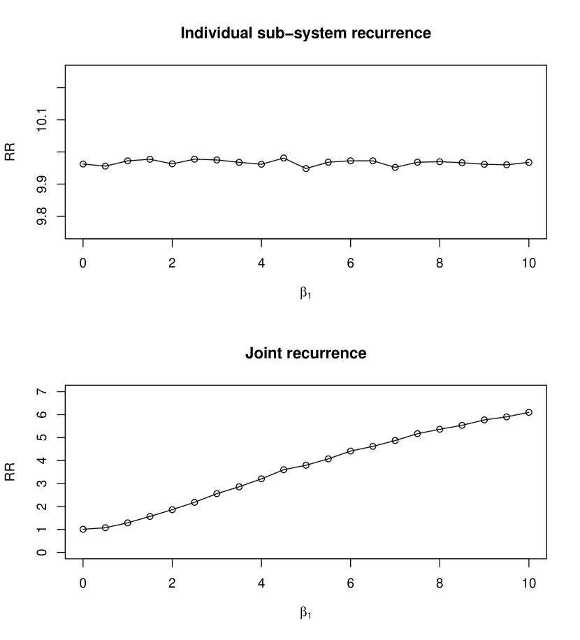
Figure 7: Recurrence rates (RR), in percent, for the individual sub-systems and the joint recurrence plot. Recurrence rate for the individual sub-systems is fixed by setting the radius parameter to a values that yields around 10 percent recurrence (top panel). For the multidimensional joint recurrence, the joint recurrence rate increases monotonically with the coupling strength $\beta_{1}$ (bottom panel).

However, this is expected given the settings in our simulation: If we have two individual RPs whose computation is based on independent samples of stochastic data (in our case: $\beta_{1}=0$), and each of these individual RPs yields at about 10 percent of recurrent point, then we expect their joint recurrence plot to yield 1 percent of recurrence. This is, because is we joint two RPs with 10 percent recurrence each, the basic odds of a joint recurrence point are 1 in 10 by mere chance. Accordingly, if we know the base recurrence rate of the two individual RPs ($RR_{1}$ and $RR_{2}$) to be joint, we can calculate the joint recurrence rate that we expect by chance ($JRR_{\text{chance}}$) simply by $JRR_{\text{chance}}=RR_{1}\cdot RR_{2}$.

Of course, for random variables that are linearly combined and do not possess interesting time dependent interactions or dynamics, and other modeling alternative exists, such as latent variable modeling (e.g., [18]). The point here is to show that the MdJRQA procedure can also be used to recover such effects for simple linear systems with stochastic data.

3 Conclusion

In the current paper, we introduced multidimensional Joint Recurrence Quantification Analysis (MdJRQA) — a method for correlating time series of different dimensionality. Based on two model systems, we showed that MdJRQA recovers coupling at the system level (i.e., when using all of the available observables) — and that this works for both non-linear and linear stochastic systems.

In applying the method it is important that the two RPs that are joined have an equal — or roughly equal — rate of recurrence. Otherwise, the RP with fewer recurrences will dictate the maximum number of possible joint recurrences, which will make the interpretation of the results more complicated. This goes particularly for data from larger samples that contain many instances of multivariate measurements.

For categorical data, the situation is more difficult, because the number of recurrences are — usually — a direct function of the data [5]. Here, normalization factors have to be applied that take into account the asymmetries in recurrence rate between the joint plots.

An important requirement for using the method is the ability to vary the coupling, or to detect a naturally occurring variation in the coupling between two systems. In our model systems, we could easily do that simply by changing the coupling constants in the models, but this is, of course, not possible with empirical data. Instead it may be possible to exert control over some properties of the systems or their interaction, and MdJRQA can then be used to detect whether such as controlled change leads to a change in the joint recurrence rate. In cases where it is impossible to apply exogenous experimental control it may instead be possible to use natural variation of the phenomenon being studied. In this case there should be some natural variation in the way the systems interact, that can be observed. Then it will be possible to perform an MdJRQA analysis of the combined system by breaking the time series down into epochs with different observed interactions — or alternatively using a countinuoiusly sliding window over the data for a windowed analysis.

4 Supplementary information

Replication scripts to reproduce all results and figures in the paper are available as a repository on GitHub: https://github.com/danm0nster/mdjrqa.

References

- [1] Drew H. Abney, Alexandra Paxton, Rick Dale and Christopher T. Kello “Complexity matching in dyadic conversation” In Journal of Experimental Psychology: General 143, 2014, pp. 2304–2315 DOI: 10.1037/xge0000021
- [2] Robin Burgess-Limerick, Bruce Abernethy and Robert J. Neal “Relative phase quantifies interjoint coordination” In Journal of Biomechanics 26.1, 1993, pp. 91–94 DOI: 10.1016/0021-9290(93)90617-N
- [3] Moreno I. Coco et al. “The R Journal: Unidimensional and Multidimensional Methods for Recurrence Quantification Analysis with crqa” In The R Journal 13.1, 2021, pp. 145–163 DOI: 10.32614/RJ-2021-062
- [4] Cassandra L. Crone et al. “Synchronous vs. non-synchronous imitation: Using dance to explore interpersonal coordination during observational learning” In Human Movement Science 76, 2021, pp. 102776 DOI: 10.1016/j.humov.2021.102776
- [5] Rick Dale, Anne S. Warlaumont and Daniel C. Richardson “Nominal cross recurrence as a generalized lag sequential analysis for behavioral streams” In International Journal of Bifurcation and Chaos 21.04, 2011, pp. 1153–1161 DOI: 10.1142/S0218127411028970
- [6] Didier Delignières, Zainy M.. Almurad, Clément Roume and Vivien Marmelat “Multifractal signatures of complexity matching” In Experimental Brain Research 234.10, 2016, pp. 2773–2785 DOI: 10.1007/s00221-016-4679-4
- [7] J.-P. Eckmann, S. Kamphorst and D. Ruelle “Recurrence Plots of Dynamical Systems” In Europhysics Letters (EPL) 4.9, 1987, pp. 973–977 DOI: 10.1209/0295-5075/4/9/004
- [8] Armin Fuchs and J.. Scott Kelso “Coordination Dynamics and Synergetics: From Finger Movements to Brain Patterns and Ballet Dancing” In Complexity and Synergetics Cham: Springer International Publishing, 2018, pp. 301–316 DOI: 10.1007/978-3-319-64334-2_23
- [9] Biyu J. He “Scale-Free Properties of the Functional Magnetic Resonance Imaging Signal during Rest and Task” In Journal of Neuroscience 31.39, 2011, pp. 13786–13795 DOI: 10.1523/JNEUROSCI.2111-11.2011
- [10] Espen A.. Ihlen and Beatrix Vereijken “Interaction-dominant dynamics in human cognition: Beyond fluctuation” In Journal of Experimental Psychology: General 139, 2010, pp. 436–463 DOI: 10.1037/a0019098
- [11] Christopher T. Kello, Gregory G. Anderson, John G. Holden and Guy C. Van Orden “The Pervasiveness of 1/f Scaling in Speech Reflects the Metastable Basis of Cognition” In Cognitive Science 32.7, 2008, pp. 1217–1231 DOI: 10.1080/03640210801944898
- [12] Nikita Kuznetsov and Sebastian Wallot “Effects of Accuracy Feedback on Fractal Characteristics of Time Estimation” In Frontiers in Integrative Neuroscience 5, 2011 DOI: 10.3389/fnint.2011.00062
- [13] Edward N. Lorenz “Deterministic Nonperiodic Flow” In Journal of the Atmospheric Sciences 20.2, 1963, pp. 130–141 DOI: 10.1175/1520-0469(1963)020<0130:DNF>2.0.CO;2
- [14] Vivien Marmelat and Didier Delignières “Strong anticipation: complexity matching in interpersonal coordination” In Experimental Brain Research 222.1, 2012, pp. 137–148 DOI: 10.1007/s00221-012-3202-9
- [15] Norbert Marwan, M. Carmen Romano, Marco Thiel and Jürgen Kurths “Recurrence plots for the analysis of complex systems” In Physics Reports 438.5, 2007, pp. 237–329 DOI: 10.1016/j.physrep.2006.11.001
- [16] Norbert Marwan and Jürgen Kurths “Nonlinear analysis of bivariate data with cross recurrence plots” In Physics Letters A 302.5, 2002, pp. 299–307 DOI: 10.1016/S0375-9601(02)01170-2
- [17] Naama Mayseless, Grace Hawthorne and Allan L. Reiss “Real-life creative problem solving in teams: fNIRS based hyperscanning study” In NeuroImage 203, 2019, pp. 116161 DOI: 10.1016/j.neuroimage.2019.116161
- [18] John J. McArdle “Latent Variable Modeling of Differences and Changes with Longitudinal Data” In Annual Review of Psychology 60.1, 2009, pp. 577–605 DOI: 10.1146/annurev.psych.60.110707.163612
- [19] Erika Nelson-Wong, Sam Howarth, David A. Winter and Jack P. Callaghan “Application of Autocorrelation and Cross-correlation Analyses in Human Movement and Rehabilitation Research” In Journal of Orthopaedic & Sports Physical Therapy 39.4, 2009, pp. 287–295 DOI: 10.2519/jospt.2009.2969
- [20] Alexanra Paxton, Drew H. Abney, Christopher T. Kello and Rick K. Dale “Network Analysis of Multimodal, Multiscale Coordination in Dyadic Problem Solving” In Proceedings of the Annual Meeting of the Cognitive Science Society 36.36, 2014 URL: https://escholarship.org/uc/item/7xz2z06w
- [21] Verónica C. Ramenzoni et al. “Joint action in a cooperative precision task: nested processes of intrapersonal and interpersonal coordination” In Experimental Brain Research 211.3, 2011, pp. 447–457 DOI: 10.1007/s00221-011-2653-8
- [22] M. Romano, Marco Thiel, Jürgen Kurths and Werner Bloh “Multivariate recurrence plots” In Physics Letters A 330.3, 2004, pp. 214–223 DOI: 10.1016/j.physleta.2004.07.066
- [23] J.. Scholz and J… Kelso “Intentional Switching Between Patterns of Bimanual Coordination Depends on the Intrinsic Dynamics of the Patterns” In Journal of Motor Behavior 22.1, 1990, pp. 98–124 DOI: 10.1080/00222895.1990.10735504
- [24] Kevin Shockley, Matthew Butwill, Joseph P Zbilut and Charles L Webber “Cross recurrence quantification of coupled oscillators” In Physics Letters A 305.1, 2002, pp. 59–69 DOI: 10.1016/S0375-9601(02)01411-1
- [25] Damian G. Stephen, Rebecca A. Boncoddo, James S. Magnuson and James A. Dixon “The dynamics of insight: Mathematical discovery as a phase transition” In Memory & Cognition 37.8, 2009, pp. 1132–1149 DOI: 10.3758/MC.37.8.1132
- [26] George Sugihara et al. “Detecting Causality in Complex Ecosystems” In Science 338.6106, 2012, pp. 496–500 DOI: 10.1126/science.1227079
- [27] Floris Takens “Detecting strange attractors in turbulence” In Lecture Notes in Mathematics 898, 1981, pp. 366–381 DOI: 10.1007/BFb0091924
- [28] Bruce Thompson “Canonical Correlation Analysis: Uses and Interpretation” SAGE, 1984
- [29] Erik Vanhatalo and Murat Kulahci “Impact of Autocorrelation on Principal Components and Their Use in Statistical Process Control” In Quality and Reliability Engineering International 32.4, 2016, pp. 1483–1500 DOI: 10.1002/qre.1858
- [30] Sebastian Wallot “Multidimensional Cross-Recurrence Quantification Analysis (MdCRQA) – A Method for Quantifying Correlation between Multivariate Time-Series” In Multivariate Behavioral Research 54.2, 2019, pp. 173–191 DOI: 10.1080/00273171.2018.1512846
- [31] Sebastian Wallot, RIccardo Fusaroli, Kristian Tylen and Else-Marie Jegindø “Using complexity metrics with R-R intervals and BPM heart rate measures” In Frontiers in Physiology 4, 2013 DOI: doi.org/10.3389/fphys.2013.00211
- [32] Sebastian Wallot and Dan Mønster “Calculation of Average Mutual Information (AMI) and False-Nearest Neighbors (FNN) for the Estimation of Embedding Parameters of Multidimensional Time Series in Matlab” In Frontiers in Psychology 9, 2018 URL: https://www.frontiersin.org/article/10.3389/fpsyg.2018.01679
- [33] Sebastian Wallot, Andreas Roepstorff and Dan Mønster “Multidimensional Recurrence Quantification Analysis (MdRQA) for the Analysis of Multidimensional Time-Series: A Software Implementation in MATLAB and Its Application to Group-Level Data in Joint Action” In Frontiers in Psychology 7, 2016 DOI: 10.3389/fpsyg.2016.01835
- [34] C.. Webber and J.. Zbilut “Dynamical assessment of physiological systems and states using recurrence plot strategies” In Journal of Applied Physiology 76.2, 1994, pp. 965–973 DOI: 10.1152/jappl.1994.76.2.965
- [35] Joseph P. Zbilut, Alessandro Giuliani and Charles L. Webber “Detecting deterministic signals in exceptionally noisy environments using cross-recurrence quantification” In Physics Letters A 246.1, 1998, pp. 122–128 DOI: 10.1016/S0375-9601(98)00457-5