Severity classification of ground-glass opacity via
2-D convolutional neural networks and lung CTs:
a 3-day exploration

Lisa Y. W. Tang

Abstract

Ground-glass opacity is a hallmark of numerous lung diseases, including patients with COVID19 and pneumonia, pulmonary fibrosis, and tuberculosis. This brief note presents experimental results of a proof-of-concept framework that got implemented and tested over three days as driven by the third challenge entitled ”COVID-19 Competition”, hosted at the AI-Enabled Medical Image Analysis Workshop of the 2023 IEEE International Conference on Acoustics, Speech and Signal Processing (ICASSP 2023). Using a newly built virtual environment (created on March 17, 2023), we investigated various pre-trained two-dimensional convolutional neural networks (CNN) such as Dense Neural Network, Residual Neural Networks, and Vision Transformers, as well as the extent of fine-tuning each architecture would require. Based on empirical experiments, we opted to fine-tune them using ADAM’s optimization algorithm with a standard learning rate of 0.001 for all CNN architectures and apply early-stopping whenever the validation loss reached a plateau. For each trained CNN, the model state with the best validation accuracy achieved during training was stored and later reloaded for new classifications of unseen samples drawn from the validation set provided by the challenge organizers. According to the organizers, few of these 2D CNNs yielded performance comparable to the baseline developed by the organizers. As part of the challenge requirement, the source code produced during the course of this exercise is posted at https://github.com/lisatwyw/cov19. We also hope that other researchers will find this prototype of few Python files based on PyTorch 1.13.1 and TorchVision 0.14.1 approachable for their own work.

Keywords: Computed Tomography; pulmonary parenchymal involvement; ground-glass opacity severity; AlexNet; DenseNet; InceptionNet; Residual Network; Wide Residual Network; SqueezeNet; VisionTransform; VGG

1 Introduction

Ground-glass opacity (GGO) as captured in lung computed tomography scans (CTs) is a hallmark of numerous lung diseases and typically signifies lung consolidation [1, 2]. The extent of GGO observed in lung scans is one approach for severity assessment (known as ‘grading’) that has been used in clinical practice to facilitate the triage of patients in hospitals and acute care centres, albeit the manual process of grading by visual inspection of lung scans is laborious and time-consuming.

With the advent of deep convolutional neural networks (CNNs), computer-automated and/or computer-assisted classification of image volumes may now be done with high efficiency and accuracy. Countless studies from the past five years, e.g. [4, 20], have further shown the success of transfer learning of CNNs trained using three-channel two-dimensional inputs. Accordingly, we approach severity classification of GGO similarly to leverage off-the-shelf pretrained networks that could facilitate model training with training sample sizes smaller than 500. To this end, we explored the use of various CNNs architectures: AlexNet [11], VGG [18], Residual Networks [14], Wide Residual Networks [15], DenseNet [12], SqueezeNet [16] and Vision Transformers [17].

This note aims to document the initial experimental work done on the open-source dataset named “COV19CT-DB” (COVID-19 Computed Tomography Database) as part of a challenge submission to the third competition entitled “ICASSP: COVID19 severity detection challenge”. Due to time constraints (i.e. three days), we focus on the severity classification problem where the objective is to label each CT volume as either mild, moderate, severe, or critical [6]. These categories were predetermined by a pre-existing protocol where experts visually inspected each scan for GGO and manually labeled each as “mild” if less than 26% of the lung volumes were judged to capture “pulmonary parenchymal involvement”; “moderate” if the involvement as 26-50%; “severe” if involvement is 50-70%; or “critical” if involvement was greater than 75% [19].

2 Materials

The training and validation samples is derived as a subsest of a larger dataset named “COV19-CT-DB” that contains over one thousand patient samples of three-Dimensional CT chest scans as archived in lossy compression format (i.e. JPEG) [6, 5, 7, 8, 9, 10]. These CT volumes were collected from different hospitals in the United States from September 1 2020 and November 30 2021 [6]. Upon successful enrolment into the ICASSP 2023 challenge, participants were directed to four hyperlinks to OneDrive where zipped archives (.rar or .zip) could be downloaded. Upon decompression, each folder represents a patient scan, with each containing up to 300 individual CT slices in JPEG format. To this end, 430 and 101 CT scans were provided for model training and validation, respectively.

3 Methods

On a high level, we propose the deployment of pretrained convolutional neural networks (CNNs) for the classification task. For ease of optimization, our approach explores a previous framework that leveraged two-dimensional (2D) Residual Networks [4] for the identification of a lung disease. The decision to employ 2D networks was motivated by two factors: time constraints and the observation that GGO have been observed in lower lung lobes in COVID-19 patients [6].

3.1 Preprocessing

As the information on field of volume and voxel spacing are no longer accessible in the archival format provided by the challenge (i.e. JPEG), the depth of each CT volume was approximated by the file count $n$ of each scan / folder, i.e.

⬇ import subprocess output = subprocess.run([’ls’, ct_folder], stdout = subprocess.PIPE ); n = len( output.stdout.decode(’utf-8’).split() )

The axial section centered at $z$ was computed deterministically ( $z=\lfloor n*f\rceil$ ). The value of $f=0.25$ was defined based on visual inspection on a subset of the images randomly drawn from the training set. Then, three contiguous slices centered at $z$ were concatenated to form three-channel inputs of size $3\times v\times v$ where $v$ depends on the CNN model [4].

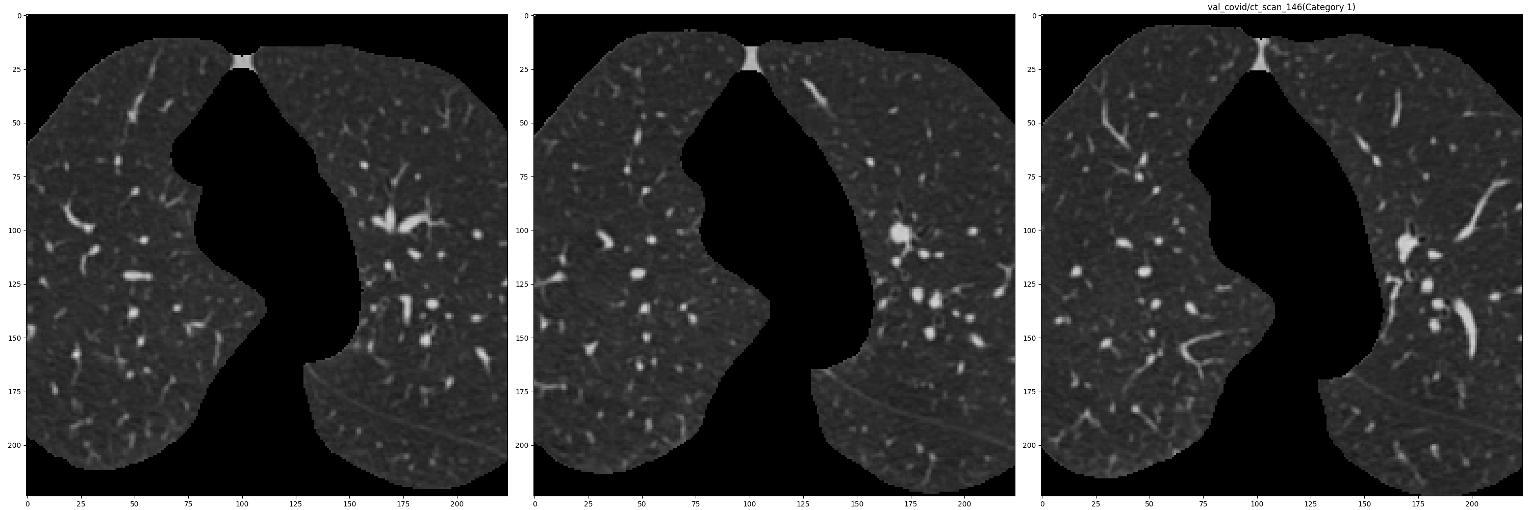
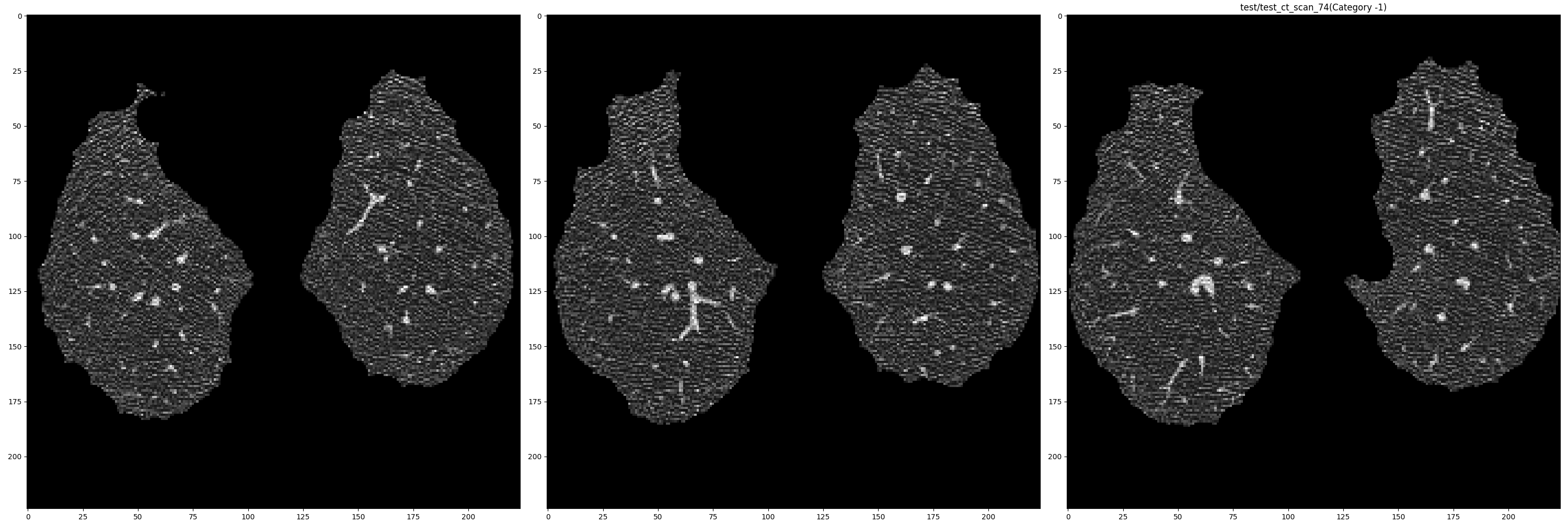
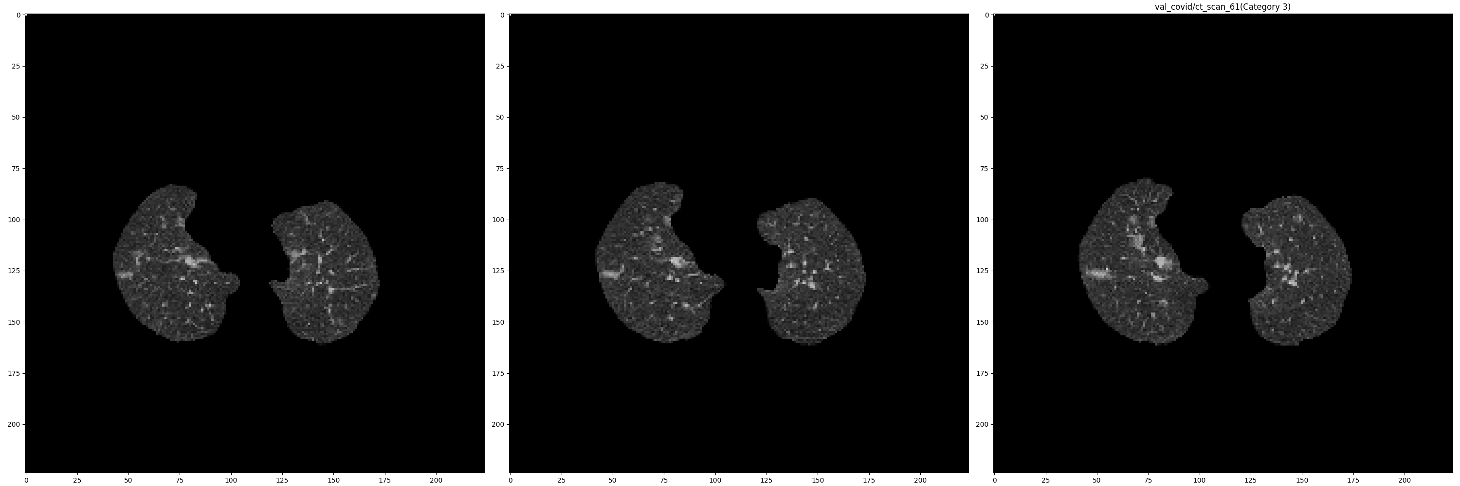
Prior to resizing, lung masks were also computed to mask out regions outside the rib cage, as shown in Figures 1-3. The implementation code of lung mask generation was adopted from an online resource [22] such that the threshold parameter is adjusted so it will operate on the compressed data as stored in the JPEG images from COV19-CT-DB, i.e.:

Figures 1-3 provide examples of the image inputs.

⬇ from skimage.segmentation import clear_border init_roi_mask = jpeg_im_slice<100 # Updated roi_mask_v0 = clear_border(init_roi_mask) …

3.2 Model-training

Each model architecture was fine-tuned over a maximum of 500 epochs. We used the categorical cross-entropy objective. For all CNN architectures, we applied early-stopping whenever the validation loss reached a plateau. Two optimization algorithms explored were Adaptive Moment Estimation (ADAM) and Stochastic Gradient Descent (SGD). For SGD, the standard setting of using momentum value of 0.9 was used. The following settings were explored initially: batch size BS= $\{16,128\}$ , optimization’s learning rate LR= $\{0.001,0.01\}$ .

3.3 Extent of fine-tuning

We initialized each CNN with pretrained weights and subsequently explored two level of network fine-tuning: allowing the network weights of all layers or only the last layer to be changed/optimized.

3.4 Evaluation metrics and model selection

For each class, we calculated the area under the receiver’s operating curve (AUROC) and the F1-macro score, i.e.

\textbf{F1-mac}=\frac{1}{K}\sum^{K}_{i=1}\frac{2\times PR_{i}\times RC_{i}}{PR_{i}+RC_{i}}

(1)

where $K$ is the number of classes ( $K=4$ severity classes of GGO) and $RC_{i}$ and $PR_{i}$ respectively denotes the precision and recall for class $i$ , i.e. $PR_{i}=\frac{TP_{i}}{TP_{i}+FP_{i}}$ and $RC_{i}=\frac{TP_{i}}{TP_{i}+FN_{i}}$ .

For each trained CNN, the state with the best validation accuracy achieved during training was selected for the evaluation of each test sample.

3.5 Evaluation protocol

We set a random subset of the training set as the internal validation set. The entire validation set of $n$ =101 was left as unseen by each CNN. The test set ( $n$ =230) was provided by the organizers a few days before the challenge deadline. The labels on the test set is blinded to participants.

		AUROC		F1-macro		Pred. class distr.
Model	Settings	Val	Unseen*	Val	Unseen*
AlexNet	BS16 SGD LR0.001	66.8	59.0	49.6	39.5	89, 31, 92, 19
AlexNet	BS32 ADAM LR0.001	66.6	59.8	51.1	34.0	61, 53, 106, 11
AlexNet	BS512 SGD LR0.001	67.1	59.0	39.9	30.9	93, 18, 120, 0
AlexNet	BS64 ADAM LR0.001	66.1	62.0	49.4	45.1	78, 41, 100, 12
DenseNet201	BS16 SGD LR0.001	62.1	59.0	42.9	38.8	80, 32, 114, 5
DenseNet201	BS32 ADAM LR0.001	63.4	63.3	46.3	46.8	57, 73, 99, 2
DenseNet201	BS512 SGD LR0.001	63.1	62.5	45.6	45.1	50, 76, 103, 2
DenseNet201	BS64 ADAM LR0.001	61.4	62.2	41.9	36.4	57, 63, 109, 2
DenseNet	BS16 ADAM LR0.001	63.8	60.1	34.8	35.9	86, 15, 130, 0
DenseNet	BS16 SGD LR0.001	63.8	60.1	34.8	35.9	86, 15, 130, 0
DenseNet	BS32 ADAM LR0.001	65.1	67.2	38.1	40.9	71, 26, 134, 0
DenseNet	BS512 SGD LR0.001	67.5	67.0	41.5	51.4	68, 46, 115, 2
DenseNet	BS64 ADAM LR0.001	65.8	63.4	39.2	37.6	58, 17, 156, 0
InceptionNet	BS16 SGD LR0.001	59.5	58.2	38.1	40.0	89, 17, 123, 2
InceptionNet	BS32 ADAM LR0.001	63.0	52.5	44.0	27.8	80, 41, 108, 2
InceptionNet	BS512 SGD LR0.001	63.7	64.3	38.6	39.5	39, 58, 134, 0
InceptionNet	BS64 ADAM LR0.001	60.8	55.1	40.7	36.3	61, 77, 91, 2
ResNet152	BS16 SGD LR0.001	63.8	54.6	36.5	28.5	76, 51, 104, 0
ResNet152	BS32 ADAM LR0.001	67.7	57.5	40.7	29.5	74, 35, 122, 0
ResNet152	BS512 SGD LR0.001	66.6	59.5	39.4	30.8	107, 50, 74, 0
ResNet152	BS64 ADAM LR0.001	65.1	56.3	38.4	28.8	81, 26, 124, 0
SqueezeNet	BS16 SGD LR0.001	68.8	58.8	42.6	32.4	74, 34, 123, 0
SqueezeNet	BS32 ADAM LR0.001	67.7	63.4	53.2	44.6	61, 68, 95, 7
SqueezeNet	BS512 SGD LR0.001	65.4	58.9	50.3	39.0	60, 54, 112, 5
SqueezeNet	BS64 ADAM LR0.001	66.5	63.8	50.5	45.2	60, 70, 94, 7
VGG	BS16 SGD LR0.001	62.5	58.5	43.9	35.4	75, 65, 81, 10
VGG	BS32 ADAM LR0.001	62.2	63.7	45.1	44.2	89, 65, 72, 5
VGG	BS512 SGD LR0.001	63.1	60.5	44.6	33.5	66, 78, 82, 5
VGG	BS64 ADAM LR0.001	63.6	58.2	46.8	33.0	92, 57, 78, 4
VTB32	BS16 SGD LR0.001	68.6	68.0	54.7	52.0	77, 45, 95, 14
VTB32	BS32 ADAM LR0.001	67.1	65.7	52.9	48.9	78, 48, 96, 9
VTB32	BS512 SGD LR0.001	63.6	61.8	45.2	40.4	78, 38, 115, 0
VTB32	BS64 ADAM LR0.001	67.0	66.6	52.6	51.3	74, 48, 96, 13
WideResNet101	BS16 SGD LR0.001	67.0	60.2	40.4	33.4	84, 27, 120, 0
WideResNet101	BS32 ADAM LR0.001	65.0	58.3	37.4	29.9	90, 16, 125, 0
WideResNet101	BS512 SGD LR0.001	65.3	57.2	48.4	31.5	73, 55, 101, 2
WideResNet101	BS64 ADAM LR0.001	62.1	58.1	32.6	29.7	89, 6, 136, 0

Table 1: Performance when model weights were fine-tuned only on the last layer. Shown are the overall and class-wise F1-scores expressed in percentages. *Performance of CNNs when evaluated the entire validation set was not observed during training. “Pred. class distr.” denotes the predicted class distribution on the test set.

		AUROC		F1-macro		Pred. class distr.
Model	Settings	Val	Unseen	Val	Unseen
AlexNet	BS16 SGD LR0.001	50.0	50.0	13.8	15.4	0, 0, 231, 0
AlexNet	BS32 ADAM LR0.001	50.0	50.0	13.8	15.4	0, 0, 231, 0
AlexNet	BS512 SGD LR0.001	42.6	46.7	23.8	21.2	0, 25, 206, 0
AlexNet	BS64 ADAM LR0.001	50.0	50.0	13.8	15.4	0, 0, 231, 0
DenseNet201	BS16 SGD LR0.001	68.3	63.4	52.9	43.1	101, 21, 95, 14
DenseNet201	BS32 ADAM LR0.001	72.1	63.1	59.4	43.7	71, 75, 74, 11
DenseNet201	BS64 ADAM LR0.001	72.2	66.4	59.3	49.4	59, 81, 85, 6
DenseNet	BS16 ADAM LR0.001	68.2	69.7	54.3	51.6	81, 64, 79, 7
DenseNet	BS16 SGD LR0.001	67.9	70.4	53.6	54.1	58, 43, 125, 5
DenseNet	BS32 ADAM LR0.001	74.7	65.7	63.5	47.6	84, 81, 58, 8
DenseNet	BS64 ADAM LR0.001	71.1	64.3	54.8	41.8	105, 15, 87, 24
InceptionNet	BS16 SGD LR0.001	68.3	61.5	51.8	38.4	107, 56, 63, 5
InceptionNet	BS32 ADAM LR0.001	73.1	66.4	60.4	48.2	86, 52, 79, 14
InceptionNet	BS64 ADAM LR0.001	66.8	58.6	45.6	32.2	115, 4, 108, 4
ResNet152	BS16 ADAM LR0.001	72.5	71.9	56.7	57.3	94, 65, 47, 25
ResNet152	BS16 SGD LR0.001	67.2	68.4	47.5	48.7	112, 70, 40, 9
ResNet152	BS32 ADAM LR0.001	68.4	65.1	52.5	47.5	87, 51, 88, 5
ResNet152	BS64 ADAM LR0.001	67.6	71.7	49.4	56.2	85, 77, 65, 4
SqueezeNet	BS16 SGD LR0.001	59.3	62.8	32.2	37.0	48, 13, 170, 0
SqueezeNet	BS32 ADAM LR0.001	63.7	61.1	38.0	34.4	61, 36, 134, 0
SqueezeNet	BS512 SGD LR0.001	67.5	65.3	41.9	39.2	61, 33, 137, 0
SqueezeNet	BS64 ADAM LR0.001	68.8	67.5	41.4	40.1	111, 34, 86, 0
VGG	BS16 SGD LR0.001	69.8	59.8	53.8	36.8	88, 46, 71, 26
VGG	BS32 ADAM LR0.001	63.7	58.5	44.9	34.4	76, 50, 86, 19
VGG	BS64 ADAM LR0.001	70.1	68.7	54.9	49.0	116, 64, 35, 16
VTB32	BS16 SGD LR0.001	62.1	64.1	42.4	46.0	84, 55, 89, 3
VTB32	BS32 ADAM LR0.001	60.8	61.8	39.2	40.1	103, 5, 116, 7
VTB32	BS512 SGD LR0.001	67.7	61.9	53.4	44.6	49, 64, 115, 3
VTB32	BS64 ADAM LR0.001	69.1	67.4	54.2	52.1	68, 43, 109, 11
WideResNet101	BS16 SGD LR0.001	69.6	62.2	54.3	42.0	120, 34, 69, 8
WideResNet101	BS32 ADAM LR0.001	68.1	65.9	52.2	49.5	33, 72, 118, 8
WideResNet101	BS64 ADAM LR0.001	68.4	63.1	50.0	44.6	80, 90, 57, 4

Table 2: Performance when all model weights were fine-tuned.

4 Results

We first examined the results of fine-tuning the models on the last layer. Table 1 reports preliminary comparisons of the accuracies (F1-macro score and area under receiver’s operating curve) achieved by individual models as evaluated on the unseen validation set. That is, all images from the validation set were not observed by the models during training. As Table 1 shows, only DenseNet and Vision Transformer (VTB32) achieved greater than 51 in F1-macro on the unseen validation set ( $n$ =101).

We next examined the results of fine-tuning the models on the all layers. Similar to the previous results, only DenseNet, ResNet152, and Vision Transformer (VTB32) achieved greater than 51 in F1-macro on the same unseen validation set, as reported in Table 2. The class-wise F1-macro scores are further reported in Table 3.

In summary, when only the training set was used ( $n$ =430) and the entire validation set was left as unseen (i.e. only used for evaluation), fine-tuning all network weights seemed to add minor improvement to the accuracy performance of DenseNet and Vision Transformers while fine-tuning ResNet152 substantially improved accuracy (F1-macro of less than 31.0 increased to greater than 56.0).

Based on these empirical results, we retrained ResNet152 using the same settings as listed in Table 3 but using both the training and validation images for model training.

NB. This section will be updated when the third-party evaluations of the two prediction files submitted to the organizers are published.

			Class-wise F1-macro
Model	Settings	Average F1-macro	Mild	Moderate	Severe	Critical
DenseNet	BS16 SGD LR0.001	54.1	100	74.4	67.6	62.8
ResNet152	BS16 ADAM LR0.001	56.2	100	79.4	68.8	71.7
VT (32-bit)	BS64 ADAM LR0.001	52.1	100	74.7	70.6	65.0

Table 3: Summary of performance metrics reported when weights of all layers were fine-tuned.

Refer to caption — Figure 1: Example training input used to fine-tune CNNs.

5 Conclusion

In this brief note, we shared empirical data that explored the feasibility of severity classification without the deployment of three-dimensional neural networks. The source code developed during the course of this experimental prototyping period is posted at https://github.com/lisatwyw/cov19. We hope that other researchers may find this quick prototype consisting of few Python files based on PyTorch 1.13.1 and TorchVision 0.14.1 approachable.

Acknowledgements

The author sincerely thank Professor Dimitrios Kollias and the organizing committee for provisioning the COV19-CT-DB dataset and hosting this exciting challenge [6, 5, 7, 8, 9, 10]. The author also expresses deep gratitude to Tong Tsui Shan and Kim Chuen Tang as well as staff of Compute Canada/Alliance Canada and Data Science Institute for their support.

References

[1] Engeler, Christopher E., Joseph H. Tashjian, Stephen W. Trenkner, and James W. Walsh. “Ground-glass opacity of the lung parenchyma: a guide to analysis with high-resolution CT.” AJR. American journal of roentgenology 160, no. 2 (1993): 249-251.
[2] Rawashdeh, M.A., Saade, C. “Radiation dose reduction considerations and imaging patterns of ground glass opacities in coronavirus: risk of over exposure in computed tomography”. Radiol med 126, 380–387 (2021). https://doi.org/10.1007/s11547-020-01271-2
[3] Saha M, Amin SB, Sharma A, Kumar TKS, Kalia RK. AI-driven quantification of ground glass opacities in lungs of COVID-19 patients using 3D computed tomography imaging. PLoS One. 2022;17(3):e0263916. Published 2022 Mar 14. doi:10.1371/journal.pone.0263916
[4] Lisa YW Tang, Harvey O Coxson, Stephen Lam, Jonathon Leipsic, Roger C Tam, and Don D Sin, “Towards large-scale case-finding: training and validation of residual networks for detection of chronic obstructive pulmonary disease using low-dose CT,” The Lancet Digital Health, vol. 2, no. 5, pp. e259–e267, 2020.
[5] Anastasios Arsenos, Dimitrios Kollias, and Stefanos Kollias, “A large imaging database and novel deep neural architecture for covid-19 diagnosis,” in 2022 IEEE 14th Image, Video, and Multidimensional Signal Pro- cessing Workshop (IVMSP). IEEE, 2022, p. 1–5.
[6] Dimitrios Kollias, Anastasios Arsenos, and Stefanos Kollias, “AI-MIA: Covid-19 detection & severity analysis through medical imaging,” arXiv preprint arXiv:2206.04732, 2022.
[7] Dimitrios Kollias, Anastasios Arsenos, Levon Soukissian, and Stefanos Kollias, “MIA-COV19d: COVID-19 detection through 3-D chest ct image analysis,” in Proceedings of the IEEE/CVF International Conference on Computer Vision, 2021, pp. 537–544.
[8] Dimitrios Kollias, N Bouas, Y Vlaxos, V Brillakis, M Seferis, Ilianna Kollia, Levon Sukissian, James Wingate, and S Kollias, “Deep transparent prediction through latent representation analysis,” arXiv preprint arXiv:2009.07044, 2020.
[9] Dimitris Kollias, Y Vlaxos, M Seferis, Ilianna Kollia, Levon Sukissian, James Wingate, and Stefanos D Kollias, “Transparent adaptation in deep medical image diagnosis.,” in TAILOR, 2020, p. 251– 267.
[10] Dimitrios Kollias, Athanasios Tagaris, Andreas Stafylopatis, Stefanos Kollias, and Georgios Tagaris, “Deep neural architectures for prediction in healthcare,” Complex & Intelligent Systems, vol. 4, no. 2, pp. 119–131, 2018.
[11] Krizhevsky, Alex, Ilya Sutskever, and Geoffrey E. Hinton. “ImageNet classification with deep convolutional neural networks.” Communications of the ACM 60, no. 6 (2017): 84-90.
[12] Huang, Gao, Zhuang Liu, Laurens Van Der Maaten, and Kilian Q. Weinberger. ”Densely connected convolutional networks.” In Proceedings of the IEEE conference on computer vision and pattern recognition, pp. 4700-4708. 2017.
[13] Szegedy, Christian, Vincent Vanhoucke, Sergey Ioffe, Jon Shlens, and Zbigniew Wojna. ”Rethinking the InceptionNet architecture for computer vision.” In Proceedings of the IEEE conference on computer vision and pattern recognition, pp. 2818-2826. 2016.
[14] He, Kaiming, Xiangyu Zhang, Shaoqing Ren, and Jian Sun. ”Deep residual learning for image recognition.” In Proceedings of the IEEE conference on computer vision and pattern recognition, pp. 770-778. 2016.
[15] Zagoruyko, Sergey, and Nikos Komodakis. ”Wide residual networks.” arXiv preprint arXiv:1605.07146 (2016).
[16] Iandola, Forrest N., Song Han, Matthew W. Moskewicz, Khalid Ashraf, William J. Dally, and Kurt Keutzer. ”SqueezeNet: AlexNet-level accuracy with 50x fewer parameters and¡ 0.5 MB model size.” arXiv preprint arXiv:1602.07360 (2016).
[17] Dosovitskiy, Alexey, Lucas Beyer, Alexander Kolesnikov, Dirk Weissenborn, Xiaohua Zhai, Thomas Unterthiner, Mostafa Dehghani et al. ”An image is worth 16x16 words: Transformers for image recognition at scale.” arXiv preprint arXiv:2010.11929 (2020).
[18] Simonyan, Karen, and Andrew Zisserman. ”Very deep convolutional networks for large-scale image recognition.” arXiv preprint arXiv:1409.1556 (2014).
[19] Sergey P Morozov, Anna E Andreychenko, Ivan A Blokhin, Pavel B Gelezhe, Anna P Gonchar, Alexan- der E Nikolaev, Nikolay A Pavlov, Valeria Yu Chernina, and Victor A Gombolevskiy, “MosMedData: data set of 1110 chest CT scans performed during the COVID-19 epidemic,” Digital Diagnostics, vol. 1, no. 1, pp. 49–59, 2020.
[20] Nagur Shareef Shaik and Teja Krishna Cherukuri, “Transfer learning based novel ensemble classifier for COVID-19 detection from chest CT-scans,” Computers in Biology and Medicine, vol. 141, pp. 105127, 2022.
[21] Nathan Inkawhich, “Finetuning Torchvision Models,” https://pytorch.org/tutorials/beginner/finetuning_torchvision_models_tutorial.html, last modified 2017, accessed Mar 17, 2023.
[22] Scott Mader “DST lung segmentation algorithm,” https://www.kaggle.com/code/kmader/dsb-lung-segmentation-algorithm, last modified 2017, accessed Mar 18, 2023.

Appendix A Efforts to increase transparency and reproducibility

One huge bottleneck the author experienced was the file transfer process, which involved downloading compressed archives from OneDrive onto the author’s local computer and uploading them to a remote computing cluster (i.e. AllianceCan). Further, some of the subfolders were archived in .RAR format, which could not be unzipped on the remote cluster. As a workaround, the files were uncompressed on the author’s local computer and then subsequently uploaded to the remote cluster. These file transfers may risk lost of data files. To assist future users with ensuring data integrity of the downloaded scans, a Google sheet listing the file counts for each scan has been compiled at this link: https://docs.google.com/spreadsheets/d/1SoVfioBKj_ElEETEk7o7KK_vs6VEca8LLIYW0xXpSYY/

Severity classification of ground-glass opacity via 2-D convolutional neural networks and lung CTs: a 3-day exploration