InceptionNeXt: When Inception Meets ConvNeXt

Abstract

Inspired by the long-range modeling ability of ViTs, large-kernel convolutions are widely studied and adopted recently to enlarge the receptive field and improve model performance, like the remarkable work ConvNeXt which employs $7\times 7$ depthwise convolution. Although such depthwise operator only consumes a few FLOPs, it largely harms the model efficiency on powerful computing devices due to the high memory access costs. For example, ConvNeXt-T has similar FLOPs with ResNet-50 but only achieves $\leavevmode\nobreak\ 60\%$ throughputs when trained on A100 GPUs with full precision. Although reducing the kernel size of ConvNeXt can improve speed, it results in significant performance degradation. It is still unclear how to speed up large-kernel-based CNN models while preserving their performance. To tackle this issue, inspired by Inceptions, we propose to decompose large-kernel depthwise convolution into four parallel branches along channel dimension, i.e. small square kernel, two orthogonal band kernels, and an identity mapping. With this new Inception depthwise convolution, we build a series of networks, namely IncepitonNeXt, which not only enjoy high throughputs but also maintain competitive performance. For instance, InceptionNeXt-T achieves $1.6\times$ higher training throughputs than ConvNeX-T, as well as attains 0.2% top-1 accuracy improvement on ImageNet-1K. We anticipate InceptionNeXt can serve as an economical baseline for future architecture design to reduce carbon footprint.

1 Introduction

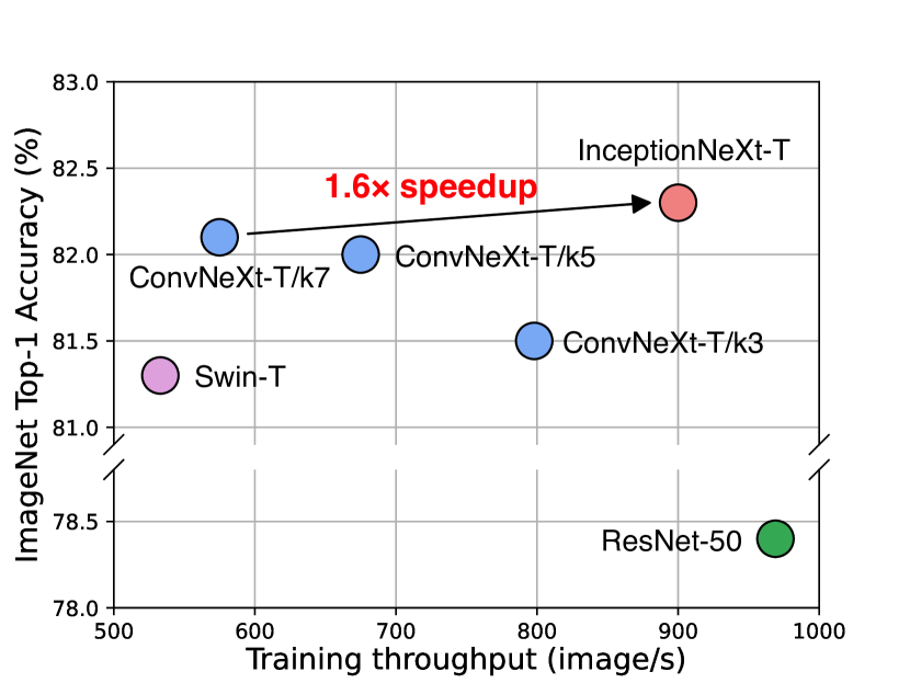
Figure 1: Trade-off between accuracy and training throughput. All models are trained under the DeiT training hyperparameters [61, 37, 38, 69]. The training throughput is measured on an A100 GPU with batch size of 128. ConvNeXt-T/k$n$ means variants with depthwise convolution kernel size of $n\times n$. InceptionNeXt-T enjoys both ResNet-50’s speed and ConvNeXt-T’s accuracy.

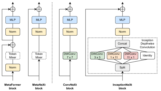
Figure 2: Block illustration of MetaFormer, MetaNext, ConvNeXt and InceptionNeXt. Similar to MetaFormer block [74], MetaNeXt is a general block abstracted from ConvNeXt [38]. MetaNeXt can be regarded as a simpler version obtained from MetaFormer by merging two residual sub-blocks into one. It is worth noting that the token mixer used in MetaNeXt cannot be too complex (e.g. self-attention [63]) or it may fail to train to converge. By specifying the token mixer as depthwise convolution or Inception depthwise convolution, the model is instantiated as ConvNeXt or InceptionNeXt block. Compared with ConvNeXt, InceptionNeXt is more efficient because it decomposes expensive large-kernel depthwise convolution into four efficient parallel branches.

Reviewing the history of deep learning [31], Convolutional Neural Networks (CNNs) [32, 33] are definitely the most popular models in computer vision. In 2012, AlexNet [30] won the ImageNet [11, 50] contest, ushering in a new era of CNNs in deep learning, especially in computer vision. Since then, numerous CNNs have emerged as trendsetters, like Network In Network [35], VGG [53], Inception Nets [56], ResNe(X)t [20, 71], DenseNet [24] and other efficient models [23, 51, 81, 58, 59].

Encouraged by the great achievement of Transformer in NLP, researchers attempt to integrate its modules or blocks into vision CNN models [67, 4, 26, 2], e.g. the representative works Non-local Neural Networks [67] and DETR [4], or even make self-attention as stand-alone primitive [48, 82]. Further, inspired by the language generative pre-training [44], Image GPT (iGPT) [6] treats pixels as tokens and adopts pure Transformer for visual self-supervised learning. However, iGPT’s ability to handle high-resolution images is limited due to the high computational cost [6]. This problem was solved by the seminal work of Vision Transformer (ViT) [16] which views image patches as tokens and proposes a simple patch embedding to generate input embeddings. ViT leverages a pure Transformer as the backbone for image classification, demonstrating remarkable performance after large-scale supervised image pre-training.

Apparently, ViT [16] further ignites the enthusiasm for Transformer’s application in computer vision. Many ViT variants [61, 76, 65, 37, 15, 73, 34], like DeiT [61] and Swin [37], are proposed and have achieved remarkable performance across a wide range of vision tasks. The superior performance of ViT-like models over traditional CNNs (e.g.Swin-T’s 81.2% v.s.ResNet-50’s 76.1% on ImageNet [37, 20, 11, 50]) leads many researchers to believe that Transformers will eventually replace CNNs and dominate the field of computer vision.

It is time for CNN to fight back. With advanced training techniques used by DeiT [61] and Swin [37], the work of “ResNet strikes back” shows that the performance of ResNet-50 can rise by 2.3%, up to 78.4% [69]. Further, ConvNeXt [38] demonstrates that with modern modules like GELU [21] activation and large kernel size similar to attention window size [37], CNN models can steadily outperform Swin Transformer [37] in various settings and tasks. ConvNeXt is not alone: More and more works have shown similar observations [13, 17, 72, 49, 36, 75, 64, 22]. Among these modern CNN models, the common key feature is the large receptive field that is usually achieved by depthwise convolution [41, 7] with large kernel size (e.g.$7\times 7$).

However, despite small FLOPs of depthwise convolution, it is actually an “expensive” operator because it brings high memory access costs and can be a bottleneck on powerful computing devices, like GPUs [40]. Moreover, as observed in [13], larger kernel sizes lead to lower speeds. As shown in Figure 1, the ConvNeXt-T with a default $7\times 7$ kernel size is $1.4\times$ slower than that with small kernel size of $3\times 3$, and is $1.8\times$ slower than ResNet-50, although they have similar FLOPs. However, using a smaller kernel size limits the receptive field, which can result in performance decrease. For example, ConvNeXt-T/k3 suffers a performance drop of $0.6\%$ top-1 accuracy on the ImageNet-1K dataset when compared to ConvNeXt-T/k7 (where k$n$ denotes a kernel size of $n\times n$).

It is still unclear how to speed up large-kernel CNNs while preserving their performance. In this paper, we aim to address this issue by building upon ConvNeXt as our baseline and improving the depthwise convolution module. Our initial finding suggests that not all input channels need to undergo the computationally expensive depthwise convolution operation [40], as demonstrated by our preliminary experiment results (see Table 10). Therefore, we propose to leave some channels unaltered and process only a portion of the channels with the depthwise convolution operation. Next, we propose to decompose large kernel of depthwise convolution into several groups of small kernels with Inception style [56, 57, 55]. Specifically, for the processing channels, $1/3$ of channels are conducted with kernel of $3\times 3$, $1/3$ are with $1\times k$ while the remaining $1/3$ are with $k\times 1$. With this new simple and cheap operator, termed as “Inception depthwise convolution”, our built model InceptionNeXt achieves a much better trade-off between accuracy and speed. For example, as shown in Figure 1, InceptionNeXt-T achieves higher accuracy than ConvNeXt-T while enjoying $1.6\times$ speedup of training throughput similar to ResNet-50.

The contributions of this paper are two-fold. Firstly, we propose Inception depthwise convolution which decomposes the expensive depthwise convolution into three convolution branches with small kernel sizes as well as a branch of identity mapping. Secondly, extensive experiments on image classification and semantic segmentation show the our model InceptionNeXt achieves a better speed-accuracy trade-off compared with ConvNeXt. We hope InceptionNeXt can serve as a new CNN baseline to speed up the research of neural architecture design.

2 Related work

2.1 Transformer v.s.CNN

Transformer [63] was introduced in 2017 for NLP tasks. Compared with LSTM, Transformer can not only train in parallel but also achieve better performance. Then many famous NLP models are built on Transformer, including GPT series [44, 45, 3, 42], BERT [12], T5 [47], and OPT [80]. For the application of the Transformer in vision tasks, Vision Transformer (ViT) is definitely the seminal work, showing that Transformer can achieve impressive performance after large-scale supervised training. Follow-up works [61, 76, 65, 66, 18] like Swin [37] continually improve model performance, achieving new state-of-the-art on various vision tasks. These results seem to tell us “Attention is all you need” [63].

But it is not that simple. ViT variants like DeiT usually adopt modern training procedures including various advanced techniques of data augmentation [10, 9, 79, 77, 83], regularization [57, 25] and optimizers [28, 39]. Wightman et al. find that with similar training procedures, the performance of ResNet can be largely improved. Besides, Yu et al. [74] argue that the general architecture instead of attention plays a key role in model performance. Han et al. [19] find by replacing attention in Swin with regular or dynamic depthwise convolution, the model can also obtain comparable performance. ConvNeXt [38], a remarkable work, modernizes ResNet into an advanced version with some designs from ViTs, and the resulting models consistently outperform Swin [37]. Other works like RepLKNet [13], VAN [17], FocalNets [72], HorNet [49], SLKNet [36], ConvFormer [75], Conv2Former [22], and InternImage [64] constantly improve performance of CNNs. Despite the high performance obtained, these models neglect efficiency, exhibiting lower speed than ConvNeXt. Actually, ConvNeXt is also not an efficient model compared with ResNet. We argue that CNN models should keep the original advantage of efficiency. Thus, in this paper, we aim to improve the model efficiency of CNNs while maintaining high performance.

2.2 Convolution with large kernels.

Well-known works, like AlexNet [30] and Inception v1 [56] already utilize large kernels up to $11\times 11$ and $7\times 7$, respectively. To improve the efficiency of large kernels, VGG [53] proposes to heavily stack $3\times 3$ convolutions while Inception v3 [57] factorizes $k\times k$ convolution into $1\times k$ and $k\times 1$ staking sequentially. For depthwise convolution, MixConv [60] splits kernels into several groups from $3\times 3$ to $k\times k$. Besides, Peng et al. find that large kernels are important for semantic segmentation and they decompose large kernels similar to Inception v3 [57]. Witnessing the success of Transformer in vision tasks [16, 65, 37], large-kernel convolution is more emphasized since it can offer a large receptive field to imitate attention [19, 38]. For example, ConvNeXt adopts kernel size of $7\times 7$ for depthwise convolution by default. To employ larger kernels, RepLKNet [13] proposes to utilize structural re-parameterization techniques [78, 14] to scale up kernel size to $31\times 31$; VAN [17] sequentially stacks large-kernel depth-wise convolution (DW-Conv) and depth-wise dilation convolution to obtain $21\times 21$ receptive filed; FocalNets employs a gating mechanism to fuse multi-level features from stacking depthwise convolutions; Recently, SLaK [36] factorizes large kernel $k\times k$ into two small non-square kernels ($k\times s$ and $s\times k$, where $s<k$). Different from these works, we do not aim to scale up larger kernels. Instead, we target efficiency and decompose large kernels in a simple and speed-friendly way while keeping comparable performance.

3 Method

Algorithm 1 Inception Depthwise Convolution (PyTorch-like Code)

⬇

import torch.nn as nn

class InceptionDWConv2d(nn.Module):

def __init__(self, in_channels, square_kernel_size=3, band_kernel_size=11, branch_ratio=1/8):

super().__init__()

gc = int(in_channels * branch_ratio) # channel number of a convolution branch

self.dwconv_hw = nn.Conv2d(gc, gc, square_kernel_size, padding=square_kernel_size//2, groups=gc)

self.dwconv_w = nn.Conv2d(gc, gc, kernel_size=(1, band_kernel_size), padding=(0, band_kernel_size//2), groups=gc)

self.dwconv_h = nn.Conv2d(gc, gc, kernel_size=(band_kernel_size, 1), padding=(band_kernel_size//2, 0), groups=gc)

self.split_indexes = (gc, gc, gc, in_channels - 3 * gc)

def forward(self, x):

# B, C, H, W = x.shape

x_hw, x_w, x_h, x_id = torch.split(x, self.split_indexes, dim=1)

return torch.cat(

(self.dwconv_hw(x_hw),

self.dwconv_w(x_w),

self.dwconv_h(x_h),

x_id),

dim=1)

3.1 MetaNeXt

Formulation of MetaNeXt Block. ConvNeXt [38] is a modern CNN model with simple architecture. For each ConvNeXt block, the input $X$ is first processed by a depthwise convolutioin to propagate information along spatial dimensions. We follow MetaFormer [74] to abstract the depthwise convolution as a token mixer which is responsible for spatial information interaction. Accordingly, as shown in the second subfigure in Figure 2, the ConvNeXt is abstracted as MetaNeXt block. Formally, in a MetaNeXt block, its input $X$ is firstly processed as

$$X^{\prime}=\mathrm{TokenMixer}(X)$$ (1)

where $X,X^{\prime}\in\mathbb{R}^{B\times C\times H\times W}$ with $B$, $C$, $H$ and $W$ denoting batch size, channel number, height and width, respectively. Then the output from the token mixer is normalized,

$$Y=\mathrm{Norm}(X^{\prime})$$ (2)

After normalization [27, 1], the resulting features are inputted into an MLP module consisting of two fully-connected layers with an activation function sandwiched between them, the same as feed-forward network in Transformer [63]. The two fully-connected layers can also be implemented by $1\times 1$ convolutions. Also, shortcut connection [20, 54] is adopted. This process can be expressed by

$$Y=\mathrm{Conv}_{1\times 1}^{rC\rightarrow C}\{\sigma[\mathrm{Conv}_{1\times 1}^{C\rightarrow rC}(Y)]\}+X,$$ (3)

where $\mathrm{Conv}_{k\times k}^{C_{i}\rightarrow C_{o}}$ means convolution with kernel size of $k\times k$, input channels of $C_{i}$ and output channels of $C_{o}$; $r$ is the expansion ratio and $\sigma$ denotes activation function.

Comparison to MetaFormer block. As shown in Figure 2, it can be found that MetaNeXt block shares similar modules with MetaFormer block [74], e.g. token mixer and MLP. Nevertheless, a critical differentiation between the two models lies in the number of shortcut connections [20, 54]. MetaNeXt block implements a single shortcut connection, whereas the MetaFormer block incorporates two, one for the token mixer and the other for the MLP. From this aspect, MetaNeXt block can be regarded as a result of merging two residual sub-blocks from MetaFormer, thereby simplifying the overall architecture. As a result, the MetaNeXt architecture exhibits a higher speed compared to MetaFormer. However, this simpler design comes with a limitation: the token mixer component in MetaNeXt cannot be complicated (e.g., Attention) as shown in our experiments (Table 3).

Instantiation to ConvNeXt. As shown in Figure 2, in ConvNeXt, the token mixer is simply implemented by a depthwise convolution,

$$X^{\prime}=\mathrm{TokenMixer}(X)=\mathrm{DWConv}_{k\times k}^{C\rightarrow C}(X)$$ (4)

where $\mathrm{DWConv}_{k\times k}^{C\rightarrow C}$ denotes depthwise convolution with kernel size of $k\times k$. In ConvNeXt, $k$ is set as 7 by default.

3.2 Inception depthwise convolution

Formulation. As illustrated in Figure 1, conventional depthwise convolution with large kernel size significantly impedes model speed. Firstly, inspired by ShuffleNetV2 [40], we find processing partial channels is also enough for single depthwise convolution layer as shown in our preliminary experiments in Appendix A. Thus, we leave partial channels unchanged and denote them as a branch of identity mapping. For the processing channels, we propose to decompose the depthwise operations with Inception style [56, 57, 55]. Inception [56] utilizes several branches of small kernels (e.g. $3\times 3$) and large kernels (e.g. $5\times 5$). Similarly, we adopt $3\times 3$ as one of our branches but avoid the large square kernels because of their slow practical speed. Instead, large kernel $k_{h}\times k_{w}$ is decomposed as $1\times k_{w}$ and $k_{h}\times 1$ inspired by Inception v3 [57].

Specifically, for input $X$, we split it into four groups along the channel dimension,

$$\begin{split}X_{\mathrm{hw}},X_{\mathrm{w}},X_{\mathrm{h}},X_{\mathrm{id}}&=\mathrm{Split}(X)\\ &=X_{:,:g},X_{:g:2g},X_{:2g:3g},X_{:3g:}\end{split}$$ (5)

where $g$ is the channel numbers of convolution branches. We can set a ratio $r_{g}$ to determine the branch channel numbers by $g=r_{g}C$. Next, the splitting inputs are fed into different parallel branches,

$$\begin{split}X^{\prime}_{\mathrm{hw}}&=\mathrm{DWConv}_{k_{s}\times k_{s}}^{g\rightarrow g}g(X_{\mathrm{hw}}),\\ X^{\prime}_{\mathrm{w}}&=\mathrm{DWConv}_{1\times k_{b}}^{g\rightarrow g}g(X_{\mathrm{w}}),\\ X^{\prime}_{\mathrm{h}}&=\mathrm{DWConv}_{k_{b}\times 1}^{g\rightarrow g}g(X_{\mathrm{h}}),\\ X^{\prime}_{\mathrm{id}}&=X_{\mathrm{id}}.\\ \end{split}$$ (6)

where $k_{s}$ denotes the small square kernel size set as 3 by default; $k_{b}$ represents the band kernel size set as 11 by default. Finally, the outputs from each branch are concatenated,

$$X^{\prime}=\mathrm{Concat}(X^{\prime}_{\mathrm{hw}},X^{\prime}_{\mathrm{w}},X^{\prime}_{\mathrm{h}},X^{\prime}_{\mathrm{id}}).$$ (7)

The illustration of InceptionNeXt block is shown in Figure 2. Moreover, its PyTorch [43] code is summarized in Algorithm 1.

Complexity. The complexity of three types of convolution, i.e., conventional, depthwise, and Inception depthwise convolution is shown in Table 1. As can be seen, Incetion depthwise convolution is much more efficient than the other two types of convolution in terms of parameter numbers of FLOPs. Inception depthwise convolution consumes parameters and FLOPs linear to both channel and kernel size. The comparison of depthwise and Inception depthwise convolutions regarding FLOPs is also clearly shown in Figure 3.

Conv. type	Params	FLOPs
Conventional conv.	$k^{2}C^{2}$	$2k^{2}C^{2}HW$
Depthwise conv.	$k^{2}C$	$2k^{2}CHW$
Inception dep. conv.	$(2k+9)C/8$	$(2k+9)CHW/4$

Table 1: Complexity of different types of convolution. For simplicity, assume input and output channels are the same, and the bias term is omitted. $k$, $C$, $H$ and $W$ denote kernel size, channel number, height and width, respectively. The parameters and FLOPs of conventional convolution and depthwise convolution are quadratic to kernel size $k$. In contrast, Inception depthwise convolution is linear to $k$.

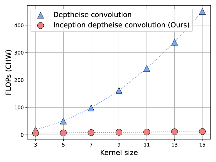
Figure 3: Comparison of FLOPs between depthwise convolution and Inception depthwise convolution. Inception depthwise convolution is much more efficient than depthwise convolution as kernel size increases.

3.3 InceptionNeXt

Based on InceptionNeXt block, we can build a series of models named InceptionNeXt. Since ConvNeXt [38] is the our main comparing baseline, we mainly follow it to build models with several sizes. Specifically, similar to ResNet [20] and ConvNeXt, InceptionNeXt also adopts 4-stage framework. The same as ConvNeXt, the numbers of 4 stages are [3, 3, 9, 3] for small size and [3, 3, 27, 3] for base size. We adopt Batch Normalization since this paper emphasizes speed. Another difference with ConvNeXt is that InceptionNeXt uses an MLP ratio of 3 in stage 4 and moves the saved parameters to the classifier, which can help reduce a few FLOPs (e.g. 3% for base size). The detailed model configurations are reported in Table 2.

Stage	#Tokens	Layer Specification		InceptionNeXt
				T	S	B
1	$\frac{H}{4}\times\frac{W}{4}$	Down- sampling	Kernel Size	$4\times 4$, stride $4$
			Embed. Dim.	$96$		$128$
		InceptionNeXt Block	Kernel size	$3\times 3$, $1\times 11$, $11\times 1$
			Conv. group ratio	1/8
			MLP Ratio	4
			# Block	3
2	$\frac{H}{8}\times\frac{W}{8}$	Down- sampling	Kernel Size	$2\times 2$, stride $2$
			Embed. Dim.	$192$		$256$
		InceptionNeXt Block	Kernel size	$3\times 3$, $1\times 11$, $11\times 1$
			Conv. group ratio	1/8
			MLP Ratio	4
			# Block	3
3	$\frac{H}{16}\times\frac{W}{16}$	Down- sampling	Kernel Size	$2\times 2$, stride $2$
			Embed. Dim.	$384$		$512$
		InceptionNeXt Block	Kernel size	$3\times 3$, $1\times 11$, $11\times 1$
			Conv. group ratio	1/8
			MLP Ratio	4
			# Block	9	27
4	$\frac{H}{32}\times\frac{W}{32}$	Down- sampling	Kernel Size	$2\times 2$, stride $2$
			Embed. Dim.	$768$		$1024$
		InceptionNeXt Block	Kernel size	$3\times 3$, $1\times 11$, $11\times 1$
			Conv. group ratio	1/8
			MLP Ratio	3
			# Block	3
Global average pooling, MLP
Parameters (M)				4.2	8.4	14.9
MACs (G)				28.1	49.4	86.7

Table 2: Configurations of InceptionNeXt models. InceptionNeXt has similar model configurations to Swin [37] and ConvNeXt [38].

Model	Params (M)	MACs (G)	Top-1 (%)
DeiT-S [61]	22	4.6	79.8
MetaNeXt-Attn	22	4.6	3.9
ConvNeXt-S (iso.) [38]	22	4.3	79.7
InceptionNeXt-S (iso.)	22	4.2	79.7
DeiT-B [61]	87	17.6	81.8
ConvNeXt-S (iso.) [38]	87	16.9	82.0
InceptionNeXt-S (iso.)	86	16.8	82.1

Table 3: Comparison among ViT, isotropic ConvNeXt and InceptionNeXt. MetaNeXt-Attn is instantiated from MetaNeXt with token mixer of self-attention [63].

Model	Mixing Type	Image (size)	Params (M)	MACs (G)	Throughput (img/second)		Top-1 (%)
					Train	Inference
DeiT-S [61]	Attn	$224^{2}$	22	4.6	1227	3781	79.8
T2T-ViT-14 [76]	Attn	$224^{2}$	22	4.8	–	–	81.5
TNT-S [18]	Attn	$224^{2}$	24	5.2	–	–	81.5
Swin-T [37]	Attn	$224^{2}$	29	4.5	564	1768	81.3
Focal-T [73]	Attn	$224^{2}$	29	4.9	–	–	82.2
ResNet-50 [20, 69]	Conv	$224^{2}$	26	4.1	969	3149	78.4
RSB-ResNet-50 [20, 69]	Conv	$224^{2}$	26	4.1	969	3149	79.8
RegNetY-4G [46, 69]	Conv	$224^{2}$	21	4.0	670	2694	81.3
FocalNet-T [72]	Conv	$224^{2}$	29	4.5	–	–	82.3
[RGB]229, 247, 255ConvNeXt-T [38]	Conv	$224^{2}$	29	4.5	575	2413 (1943)	82.1
[RGB]229, 247, 255InceptionNeXt-T (Ours)	Conv	$224^{2}$	28	4.2	901 (+57%)	2900 (+20%)	82.3 (+0.2)
T2T-ViT-19 [76]	Attn	$224^{2}$	39	8.5	–	–	81.9
PVT-Medium [65]	Attn	$224^{2}$	44	6.7	–	–	81.2
Swin-S [37]	Attn	$224^{2}$	50	8.7	359	1131	83.0
Focal-S [73]	Attn	$224^{2}$	51	9.1	–	–	83.5
RSB-ResNet-101 [20, 69]	Conv	$224^{2}$	45	7.9	620	2057	81.3
RegNetY-8G [46, 69]	Conv	$224^{2}$	39	8.0	689	1326	82.1
FocalNet-S [72]	Conv	$224^{2}$	50	8.7	–	–	83.5
[RGB]229, 247, 255ConvNeXt-S [38]	Conv	$224^{2}$	50	8.7	361	1535 (1275)	83.1
[RGB]229, 247, 255InceptionNeXt-S (Ours)	Conv	$224^{2}$	49	8.4	521 (+44%)	1750 (+14%)	83.5 (+0.4)
DeiT-B [61]	Attn	$224^{2}$	86	17.5	541	1608	81.8
T2T-ViT-24 [76]	Attn	$224^{2}$	64	13.8	–	–	82.3
TNT-B [18]	Attn	$224^{2}$	66	14.1	–	–	82.9
PVT-Large [65]	Attn	$224^{2}$	62	9.8	–	–	81.7
Swin-B [37]	Attn	$224^{2}$	88	15.4	271	843	83.5
Focal-B [73]	Attn	$224^{2}$	90	16.0	–	–	83.8
RSB-ResNet-152 [20, 69]	Conv	$224^{2}$	60	11.6	437	1457	81.8
RegNetY-16G [46, 69]	Conv	$224^{2}$	84	15.9	322	1100	82.2
RepLKNet-31B [13]	Conv	$224^{2}$	79	15.3	–	–	83.5
FocalNet-B [72]	Conv	$224^{2}$	89	15.4	–	–	83.9
[RGB]229, 247, 255ConvNeXt-B [38]	Conv	$224^{2}$	89	15.4	267	1122 (969)	83.8
[RGB]229, 247, 255InceptionNeXt-B (Ours)	Conv	$224^{2}$	87	14.9	375 (+40%)	1244 (+11%)	84.0 (+0.2)
ViT-Base/16 [16]	Attn	$384^{2}$	87	55.4	130	359	77.9
DeiT-B [61]	Attn	$384^{2}$	86	55.4	131	361	83.1
Swin-B [37]	Attn	$384^{2}$	88	47.1	104	296	84.5
RepLKNet-31B [13]	Conv	$384^{2}$	79	45.1	–	–	84.8
[RGB]229, 247, 255ConvNeXt-B [38]	Conv	$384^{2}$	89	45.0	95	393 (337)	85.1
[RGB]229, 247, 255InceptionNeXt-B (Ours)	Conv	$384^{2}$	87	43.6	139 (+46%)	428 (+9%)	85.2 (+0.1)

Table 4: Performance of models trained on ImageNet-1K. The throughputs are measured on an A100 GPU with batch size of 128 and full precision (FP32). Our environment is PyTorch 1.13.0 and NVIDIA CUDA 11.7.1. The better results of “Channel First” and “Channel Last” memory layouts are reported. The numbers in gray color are reported by ConvNeXt [38]. In our environment, ConvNeXt achieves much higher throughput than the values reported in the paper [38].

4 Experiment

Backbone	UperNet
	Params (M)	MACs (G)	mIoU (%)
Swin-T [37]	60	945	45.8
ConvNeXt-T  [38]	60	939	46.7
InceptionNeXt-T	56	933	47.9
Swin-S [37]	81	1038	49.5
ConvNeXt-S  [38]	82	1027	49.6
InceptionNeXt-S	78	1020	50.0
Swin-B [37]	121	1188	49.7
ConvNeXt-B  [38]	122	1170	49.9
InceptionNeXt-B	115	1159	50.6

Table 5: Performance of Semantic segmentation with UperNet [70] on ADE20K [84] validation set. Images are cropped to $512\times 512$ for training. The MACs are measured with input size of $512\times 2048$.

Backbone	Semantic FPN
	Params (M)	MACs (G)	mIoU (%)
ResNet-50 [20]	29	46	36.7
PVT-Small [65]	28	45	39.8
PoolFormer-S24 [74]	23	39	40.3
InceptionNeXt-T	28	44	43.1
ResNet-101 [20]	48	65	38.8
ResNeXt-101-32x4d [71]	47	65	39.7
PVT-Medium [65]	48	61	41.6
PoolFormer-S36 [74]	35	48	42.0
PoolFormer-M36 [74]	60	68	42.4
InceptionNeXt-S	50	65	45.6
PVT-Large [65]	65	80	42.1
ResNeXt-101-64x4d [71]	86	104	40.2
PoolFormer-M48 [74]	77	82	42.7
InceptionNeXt-B	85	100	46.4

Table 6: Performance of Semantic segmentation with Semantic FPN [29] on ADE20K [84] validation set. Images are cropped to $512\times 512$ for training. The MACs are measured with input size of $512\times 512$.

4.1 Image classification

Setup. For the image classification task, ImageNet-1K [11, 50] is one of the most commonly-used benchmarks, which contains around 1.3 million images in the training set and 50 thousand images in the validation set. To fairly compared with the widely-used baselines, e.g.Swin [37] and ConvNeXt [38], we mainly follow the training hyper-parameters from DeiT [61] without distillation. Specifically, the models are trained by AdamW [39] optimizer with a learning rate $lr=0.001\times\mathrm{batchsize}/1024$ ($lr=4e-3$ and $\mathrm{batchsize}=4096$ are used in this paper the same as ConvNeXt). Following DeiT, data augmentation includes standard random resized crop, horizontal flip, RandAugment [10], Mixup [79], CutMix [77], Random Erasing [83] and color jitter. For regularization, label smoothing [57], stochastic depth [25], and weight decay are adopted. Like ConvNeXt, we also use LayerScale [62], a technique to help train deep models. Our code is based on PyTroch [43] and timm [68] libraries.

Results. We compare InceptionNeXt with various state-of-the-art models, including attention-based and convolution-based models. As can be seen in Table 4, InceptionNeXt achieves highly competitive performance as well as enjoys higher speed. With similar model sizes and MACs, InceptionNeXt consistently outperforms ConvNeXt in terms of top-1 accuracy, and also exhibits higher throughput. For example, InceptionNeXt-T not only surpasses ConvNeXt-T by 0.2%, but also enjoys $1.6\times$/$1.2\times$ training/inference throughputs than ConvNeXts, similar to those of ResNet-50. That is to say, InceptionNeXt-T enjoys both ResNet-50’s speed and ConvNeXt-T’s accuracy. Moreover, following Swin and ConvNeXt, we also finetuned the model trained at the resolution of $224\times 224$ to $384\times 384$ for 30 epochs. We can see that InceptionNeXt still obtains promising performance similar to that of ConvNeXt.

Besides the 4-stage framework [53, 20, 37], another notable one is ViT-style [16] isotropic architecture which has only one stage. To match the parameters and MACs of DeiT, we construct InceptionNeXt (iso.) following ConvNeXt [38]. Specifically, for the small/base model, we set the embedding dimension as 384/768 and the block number as 18/18. Besides, we build a model called MetaNeXt-Attn which is instantiated from MetaNeXt block by specifying self-attention as token mixer. The aim of this model is to investigate whether it is possible to merge two residual sub-blocks of the Transformer block into a single one. The experiment results are shown in Table 3. It can be seen that InceptionNeXt can also perform well with the isotropic architecture, demonstrating InceptionNeXt exhibits good generalization across different frameworks. It is worth noting that MetaNeXt-Attn could not be trained to converge and only achieved an accuracy of 3.9%. This result suggests that, unlike the token mixer in MetaFormer, the token mixer in MetaNeXt cannot be too complex. If it is, the model may not be trainable.

Ablation	Variant	Params (M)	MACs (G)	Throughput		Top-1 (%)
				Train	Inference
Baseline	None (InceptionNeXt-T)	28.1	4.2	901	2900	82.3
Branch	Remove horizontal band kernel	28.0	4.2	947	3093	81.9
	Remove vertical band kernel	28.0	4.2	954	3173	81.9
	Remove small band kernel	28.0	4.2	940	3004	82.0
	horizontal and vertical band kernel in parallel $\rightarrow$ in sequence	28.1	4.2	903	2971	82.1
Band kernel size	Band kernel size 11 $\rightarrow$ 7	28.0	4.2	905	2946	82.1
	Band kernel size 11 $\rightarrow$ 9	28.1	4.2	904	2916	82.1
	Band kernel size 11 $\rightarrow$ 13	28.1	4.2	896	2895	82.0
Convolution branch ratio	Conv. branch ratio $1/8\rightarrow 1/4$	28.1	4.2	834	2499	82.2
	Conv. branch ratio $1/8\rightarrow 1/16$	28.0	4.2	936	3097	81.8

Table 7: Ablation for InceptionNeXt on ImageNet-1K classification benchmark. InceptionNeXt-T is utilized as the baseline for the ablation study. Top-1 accuracy on the validation set is reported.

4.2 Semantic segmentation

Setup. ADE20K [84], one of the commonly used scene parsing benchmarks, is used to evaluate our models on semantic segmentation task. ADE20K includes 150 fine-grained semantic categories, containing twenty thousand and two thousand images in the training set and validation set, respectively. The checkpoints trained on ImageNet-1K [11] at the resolution of $224^{2}$ are utilized to initialize the backbones. Following Swin [37] and ConvNeXt [38], we firstly evaluate InceptionNeXt with UperNet [70]. The models are trained with AdamW [39] optimizer with learning rate of 6e-5 and batch size of 16 for 160K iterations. Following PVT [65] and PoolFormer [74], InceptionNeXt is also evaluated with Semantic FPN [29]. In common practices [29, 5], for the setting of 80K iterations, the batch size is 16. Following PoolFormer [74], we increase the batch size to 32 and decrease the iterations to 40K, to speed up training. The AdamW [28, 39] optimized is adopted with a learning rate of 2e-4 and a polynomial decay schedule of 0.9 power. Our code is based on PyTorch [43] and mmsegmentation library [8].

Results. For segmentation with UpNet [70], the results are shown in Table 5. As can be seen, InceptionNeXt consistently outperforms Swin [37] and ConvNeXt [38] for different model sizes. On the setting of Semantic FPN [29] as shown in Table 6, InceptionNeXt significantly surpasses other backbones, like PVT [65] and PoolFormer [74]. These results show that InceptionNeXt also has a high potential for dense prediction tasks.

4.3 Ablation studies

We conduct ablation studies on ImageNet-1K [11, 50] using InceptionNeXt-T as baseline from the following aspects.

Branch. Inception depthwise convolution includes four branches, three convolutional ones, and identity mapping. When removing any branch of horizontal or vertical band kernel, performance significantly drops from 82.3% to 81.9%, demonstrating the importance of these two branches. This is because these two branches with band kernels can enlarge the receptive field of the model. For the branch of small square kernel size of $3\times 3$, removing it can also achieve up to 82.0% top-1 accuracy and bring higher throughput. This inspires us that if we attach more importance to the model speed, the simple version of InceptionNeXt without the square kernel of $3\times 3$ can be adopted. For the band kernel, Inception v3 mostly equips them in a sequential way. We find that this assembling method can also obtain similar performance and even a little speed up the model. A possible reason is that PyTorch/CUDA may have optimized sequential convolutions well, and we only implement the parallel branches at a high level (see Algorithm 1). We believe the parallel method will be faster when it is optimized better. Thus, parallel method for the band kernels is adopted by default.

Band kernel size. It is found the performance can be improved from kernel size 7 to 11, but it drops when the band kernel size increases to 13. This phenomenon may result from the optimization difficulty and can be solved by methods like structural re-parameterization [14, 13]. For simplicity, we just set the band kernel size as 11 by default.

Convolution branch ratio. When the ratio increases from $1/8$ to $1/4$, performance improvement can not be observed. Ma et al. [40] also point out that it is not necessary for all channels to conduct convolution. But when the ratio decreases to $1/16$, it brings a serious performance drop. It is because a smaller ratio would limit the degree of token mixing, resulting in performance drop. Thus, we set the convolution branch ratio as $1/8$ by default.

5 Conclusion and future work

In this work, we propose an effective and efficient CNN InceptionNeXt architecture that enjoys a better trade-off between the practical speed and the performance than previous network architectures. InceptionNeXt decomposes large-kernel depthwise convolution along channel dimension into four parallel branches, including identity mapping, a small square kernel, and two orthogonal band kernels. All these four branches are much more computationally efficient than a large-kernel depthwise convolution in practice, and can also work together to have a large spatial receptive field for good performance. Extensive experimental results demonstrate the superior performance and also the high practical efficiency of InceptionNeXt.

We also notice the speed-up ratios of InceptionNeXt in inference is smaller than that during training. In the future, we will dig into the different speed-up ratios during training and inference, and hope to find a way to further improve the speed-up ratio of InceptionNeXt over previous network architectures in inference.

Appendix A Preliminary experiments based on ConvNeXt-T

We conducted preliminary experiments based on ConvNeXt-T and the results are shown in Table 10. Firstly, the kernel size of depthwise convolution is reduced from $7\times 7$ to $3\times 3$. Compared to the model with kernel size of $7\times 7$, the one with kernel size of $3\times 3$ has $1.4\times$ training throughput, but it suffers a significant performance drop from 82.1% to 81.5%. Next, inspired by ShuffleNet V2 [40], we only feed partial input channels into depthwise convolution while the remaining ones keep unchanged. The number of processed input channels is controlled by a ratio. It is found that when the ratio is reduced from 1 to $1/4$, the training throughput can be further improved while the performance almost maintains. For inference throughput, significant improvement can not be observed. A possible reason is that our current code is implemented at API level and has not been optimized at low level.

Appendix B Hyper-parameters

B.1 ImageNet-1K image classification

On ImageNet-1K [11, 50] classification benchmark, we adopt the hyper-parameters shown in Table 8 to train InceptionNeXt at the input resolution of $224^{2}$ and fine-tune it at $384^{2}$. Our code is implemented by PyTorch [43] based on timm library [68].

B.2 Semantic segmentation

For ADE20K [84] semantic segmentation, we utilize ConvNeXt as the backbone with UpNet [70] following the configs of Swin [37], and FPN [29] following the configs of PVT [65] and PoolFormer [74]. The backbone is initialized by checkpoints pre-trained on ImageNet-1K at the resolution of $224^{2}$. The peak stochastic depth rates of the InceptionNeXt backbone are shown in Table 9. Our implementation is based on PyTorch [43] and mmsegmentation library [8].

Appendix C Qualitative results

Grad-CAM [52] is employed to visualize the activation maps of different models trained on ImageNet-1K, including RSB-ResNet-50 [20, 69], Swin-T [37], ConvNeXt-T [38] and our InceptionNeXt-T. The results are shown in Figure 4. Compared with other models, InceptionNeXt-T locates key parts more accurately with smaller activation areas.

	InceptionNeXt
	Train			Finetune
	T	S	B	B
Input resolution	$224^{2}$			$384^{2}$
Epochs	300			30
Batch size	4096			1024
Optimizer	AdamW			AdamW
Adam $\epsilon$	1e-8			1e-8
Adam $(\beta_{1},\beta_{2})$	(0.9, 0.999)			(0.9, 0.999)
Learning rate	4e-3			5e-5
Learning rate decay	Cosine			Cosine
Gradient clipping	None			None
Warmup epochs	20			None
Weight decay	0.05			0.05
Rand Augment	9/0.5			9/0.5
Repeated Augmentation	off			off
Cutmix	1.0			1.0
Mixup	0.8			0.8
Cutmix-Mixup switch prob	0.5			0.5
Random erasing prob	0.25			0.25
Label smoothing	0.1			0.1
Peak stochastic depth rate	0.1	0.3	0.4	0.7
Dropout in classifier	0.0			0.5
LayerScale initialization	1e-6			Pre-trained
Random erasing prob	0.25			0.25
EMA decay rate	None			0.9999

Table 8: Hyper-parameters of InceptionNeXt on ImageNet-1K image classification.

Method	InceptionNeXt stochastic depth rate
	T	S	B
UperNet [70]	0.2	0.3	0.4
FPN [29]	0.1	0.2	0.2

Table 9: Stochasic depth rate of InceptionNeXt backbone with UperNet and FPN for ADE20K semantic segmentation.

Kernel size of DWConv	Convolution ratio	Params (M)	MACs (G)	Throughput		Top-1 (%)
				Train	Inference
$7\times 7$	1.0	28.6	4.5	575	2413	82.1*
$5\times 5$	1.0	28.4	4.4	675	2704	82.0
$3\times 3$	1.0	28.3	4.4	798	2802	81.5
$3\times 3$	$1/2$	28.3	4.4	818	2740	81.4
$3\times 3$	$3/8$	28.3	4.4	847	2762	81.4
$3\times 3$	$1/4$	28.3	4.4	871	2808	81.3
$3\times 3$	$1/8$	28.3	4.4	901	2833	80.8
$3\times 3$	$1/16$	28.3	4.4	916	2846	80.1

Table 10: Preliminary experiments based on ConvNeXt-T. Convolution ratio means the ratio of channels to be processed by depthwise convolution while the other channels keep unchanged. Throughputs are measured on an A100 GPU with batch size of 128 and full precision (FP32). * The result is reported in ConvNeXt paper [38].

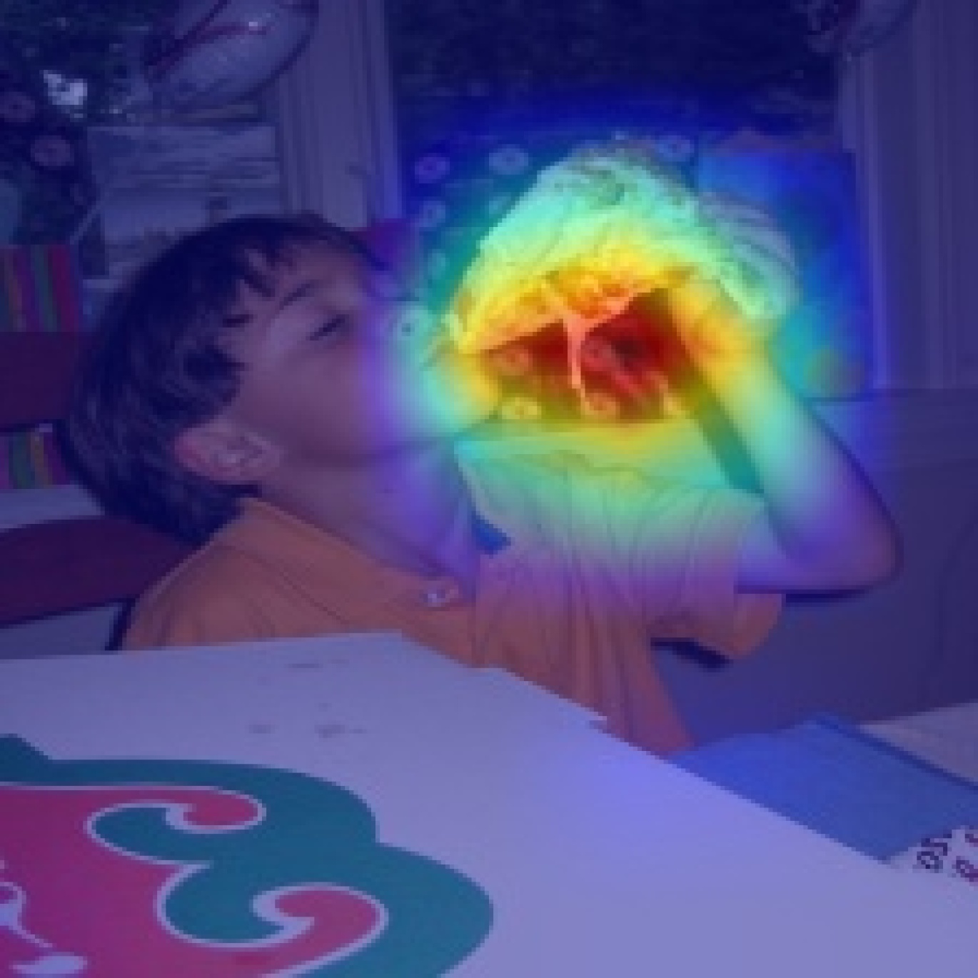
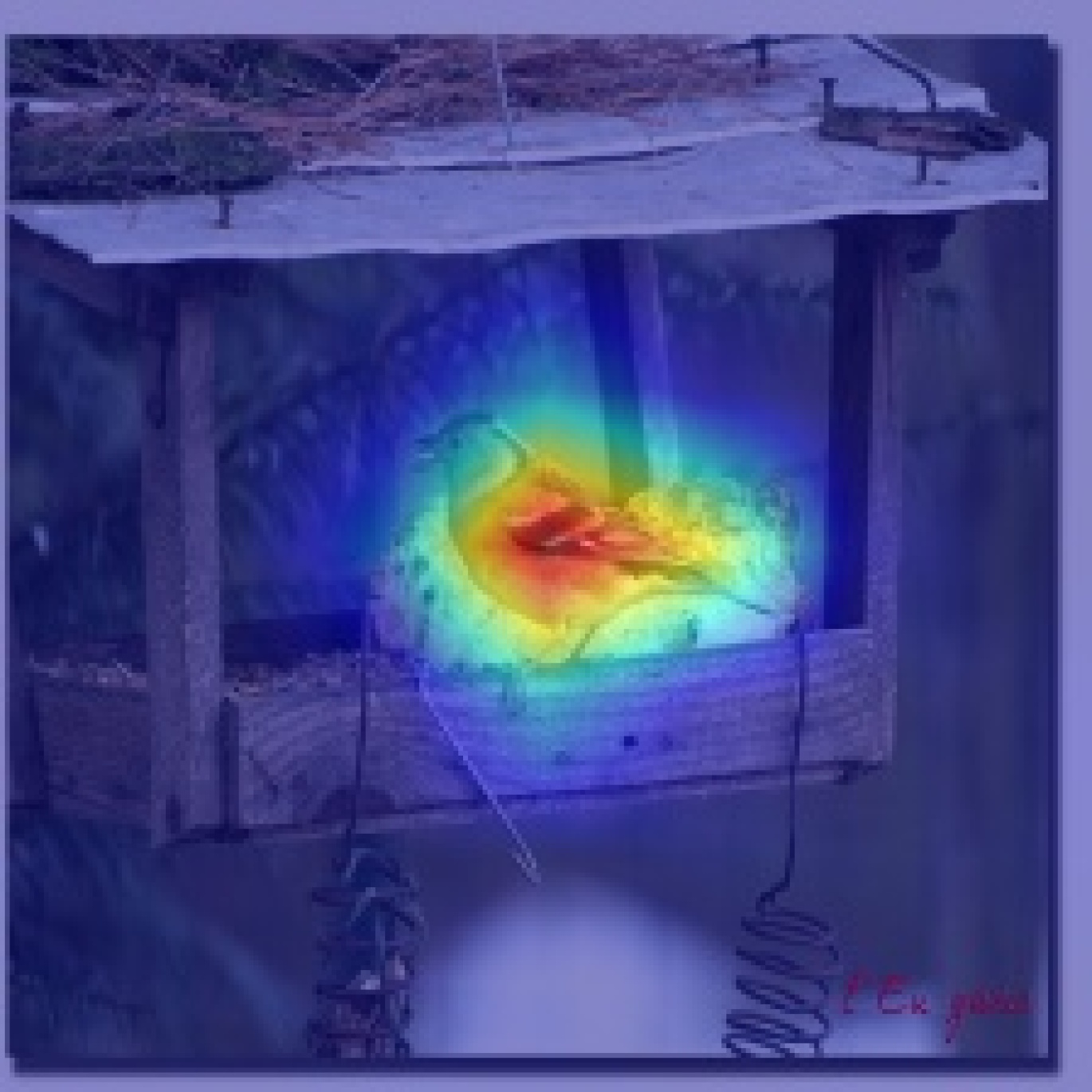
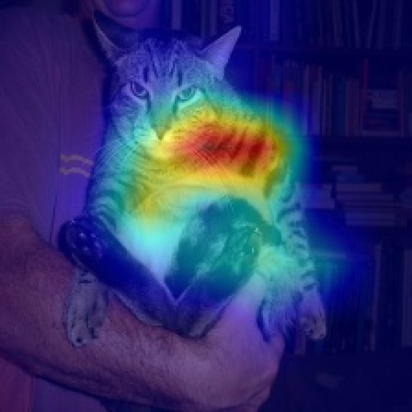
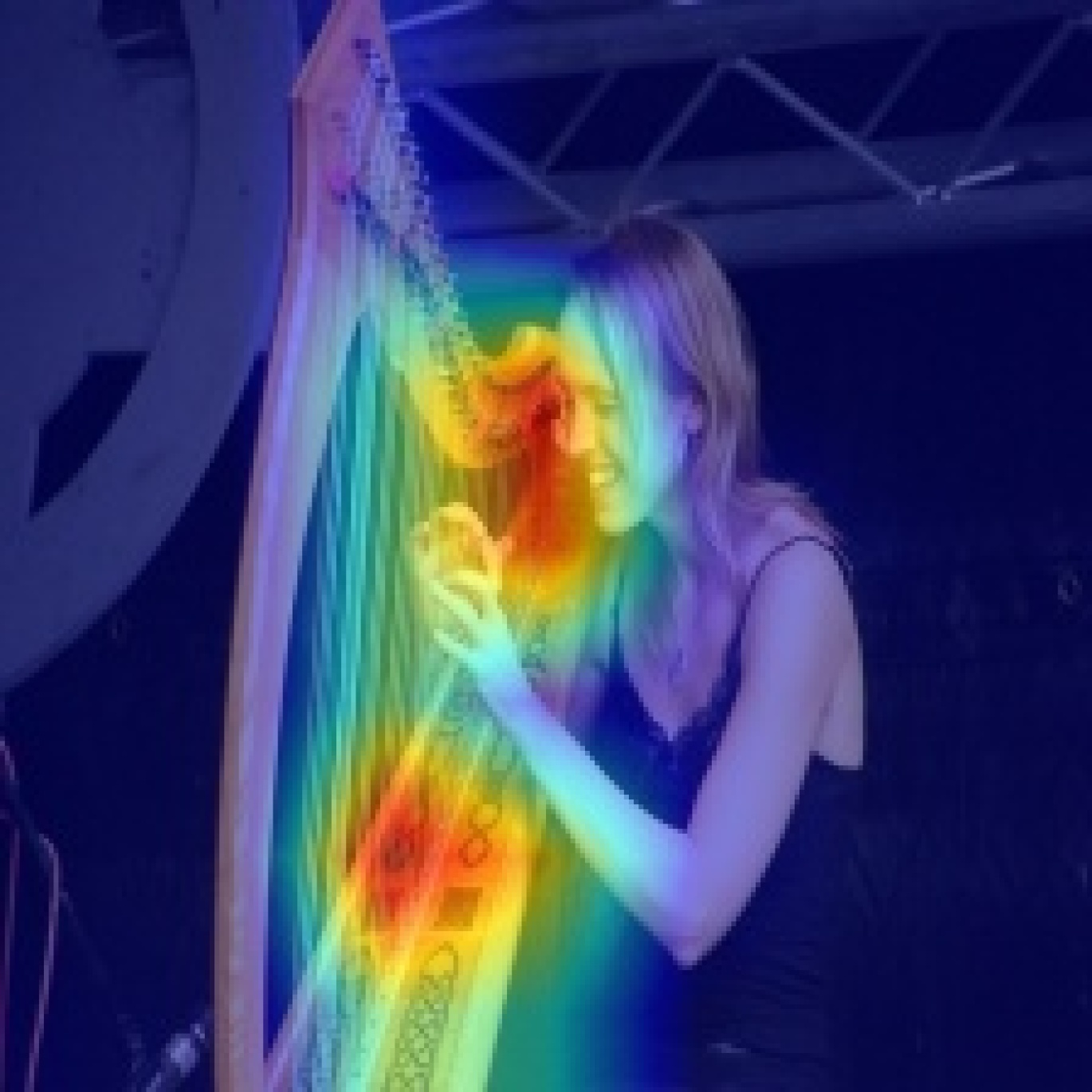
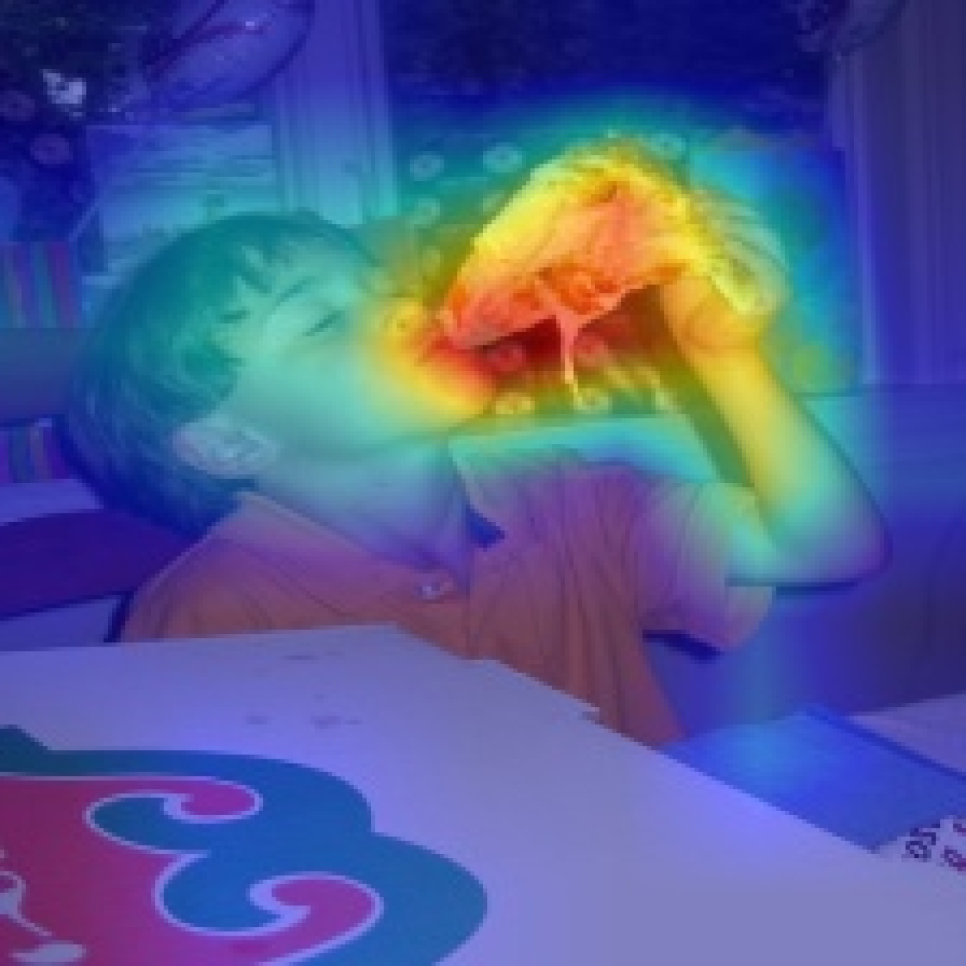
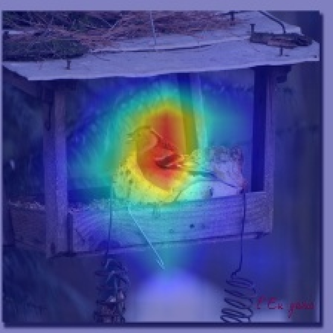
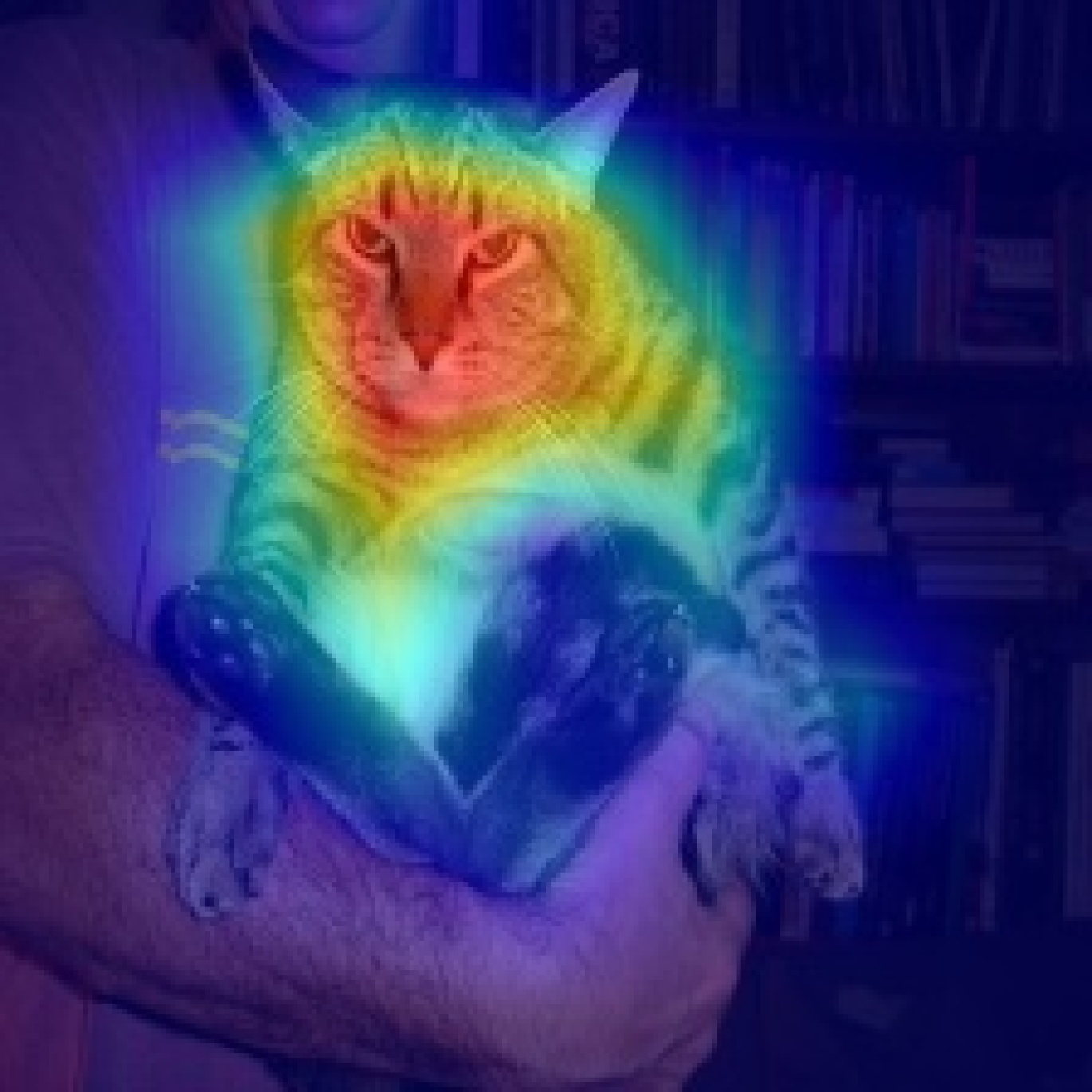
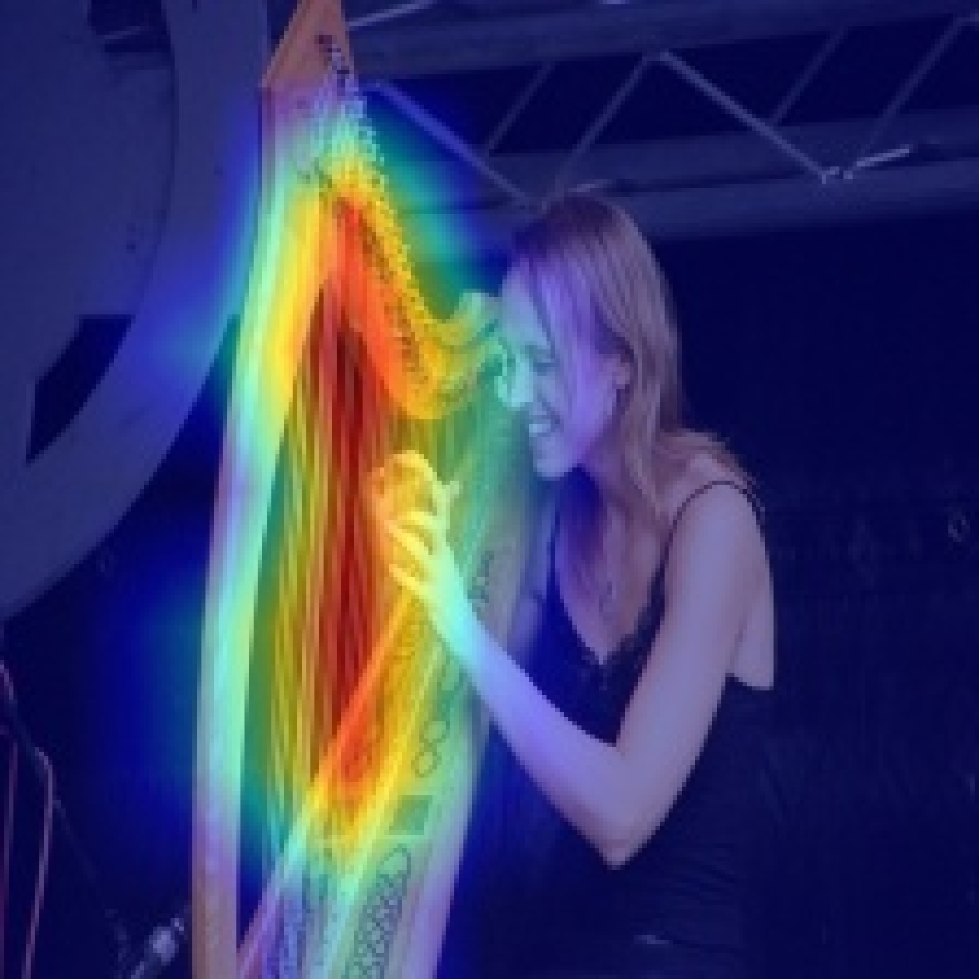
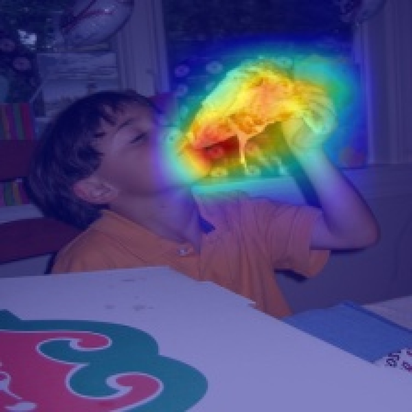
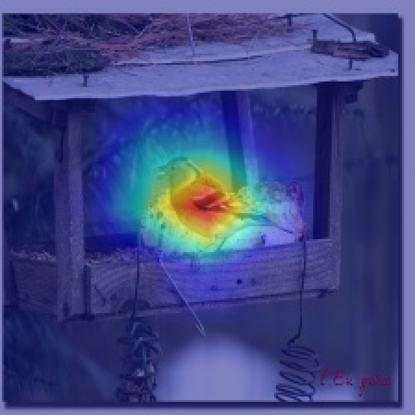
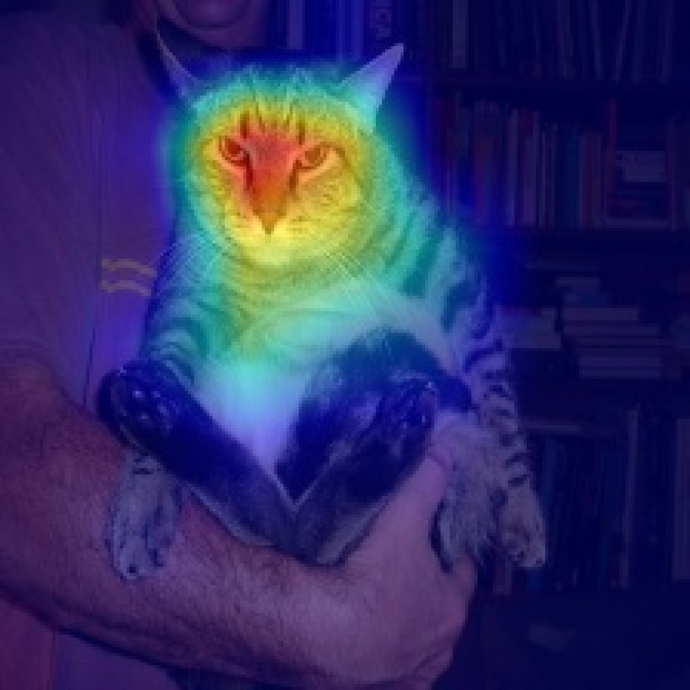
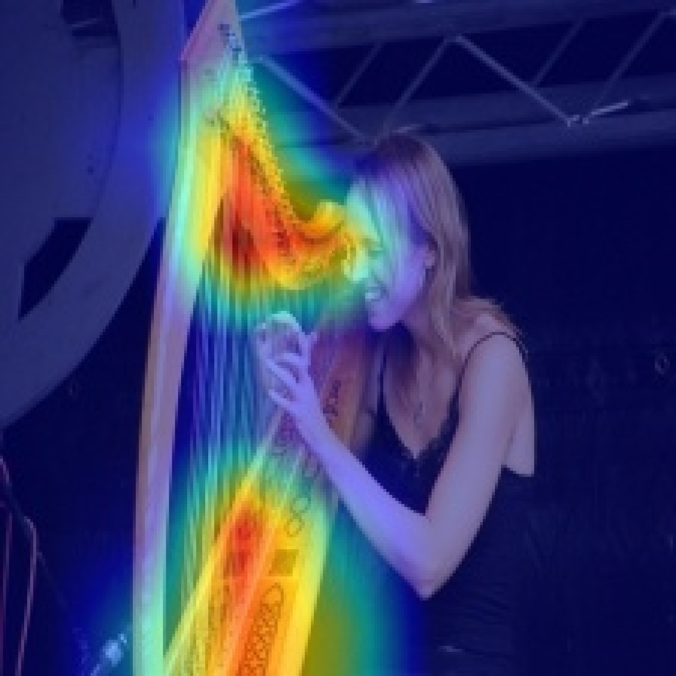
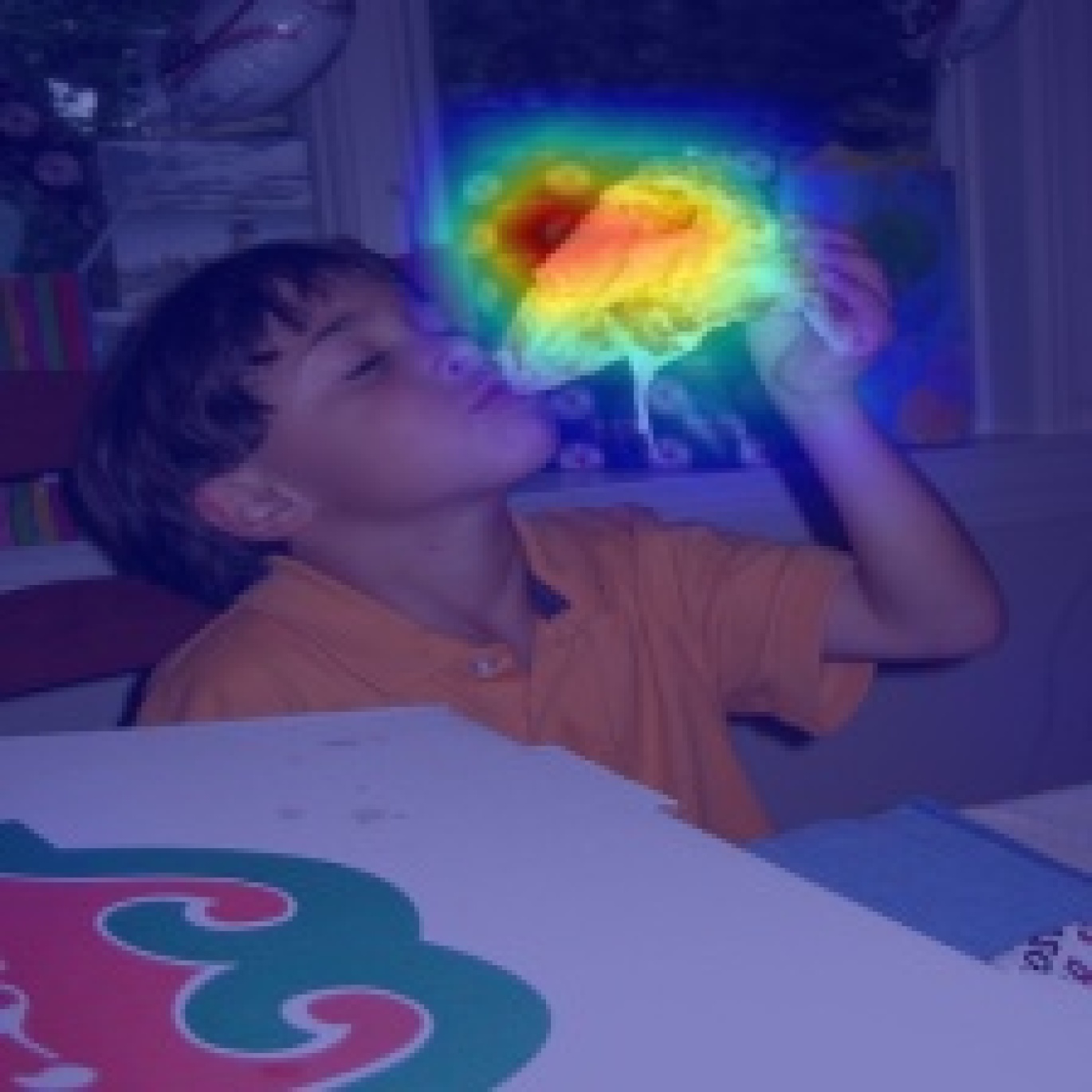
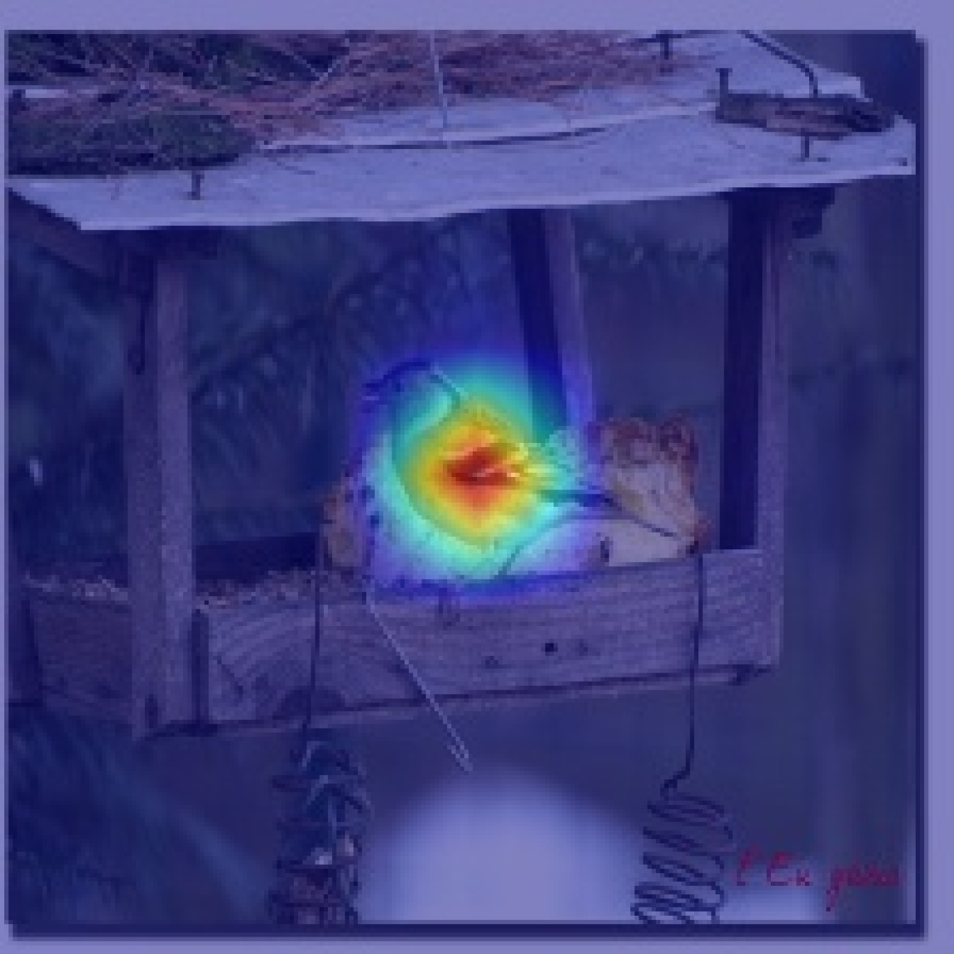
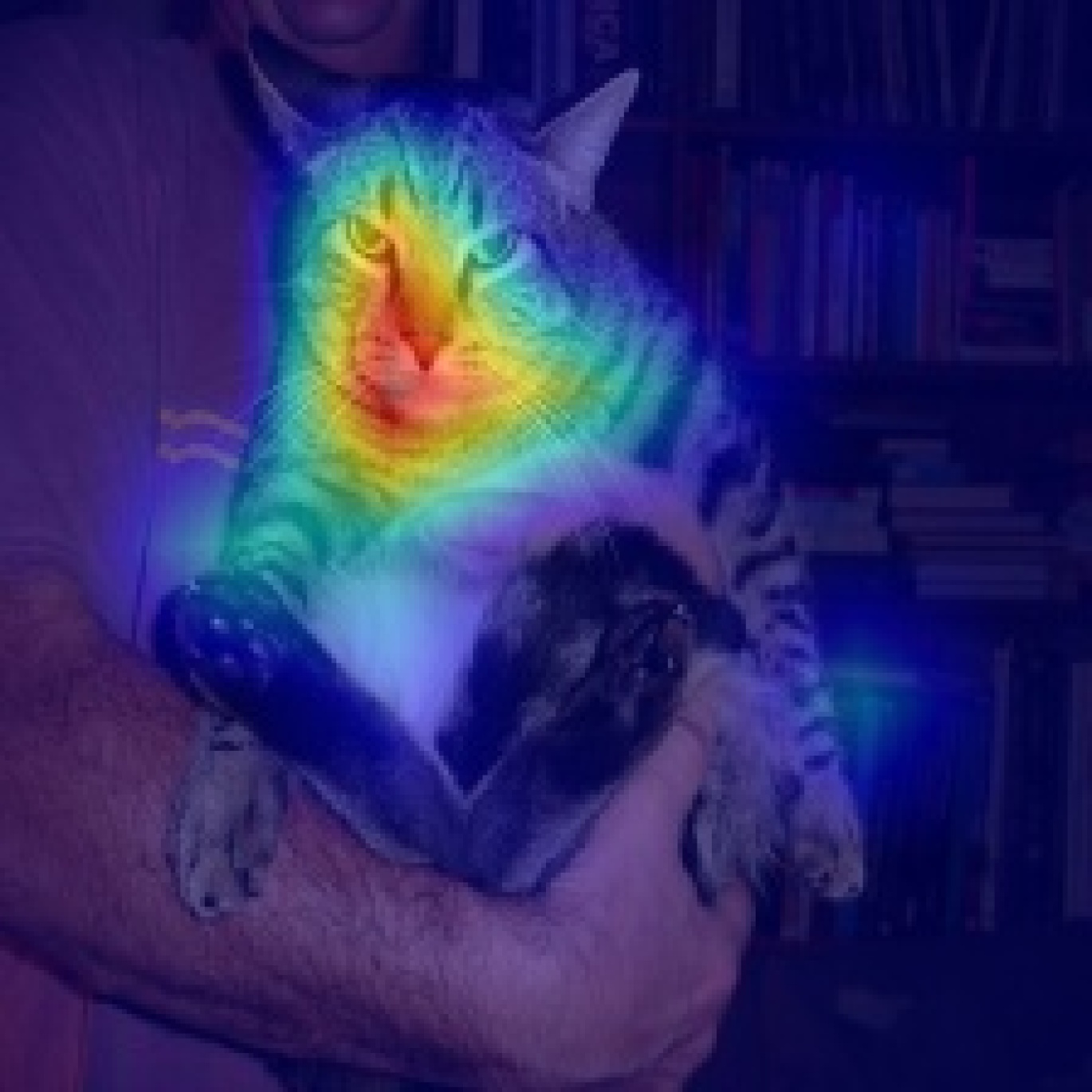
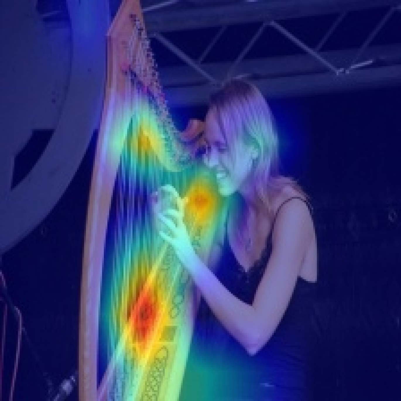
Input     RSB-ResNet-50 [20, 69]   Swin-T [61]        ConvNeXt-T [38]      InceptionNeXt-T

Figure 4: Grad-CAM [52] activation maps of different models trained on ImageNet-1K. The visualized images are from the validation set of ImageNet-1K.

References

- [1] Jimmy Lei Ba, Jamie Ryan Kiros, and Geoffrey E Hinton. Layer normalization. arXiv preprint arXiv:1607.06450, 2016.
- [2] Irwan Bello, Barret Zoph, Ashish Vaswani, Jonathon Shlens, and Quoc V Le. Attention augmented convolutional networks. In Proceedings of the IEEE/CVF international conference on computer vision, pages 3286–3295, 2019.
- [3] Tom Brown, Benjamin Mann, Nick Ryder, Melanie Subbiah, Jared D Kaplan, Prafulla Dhariwal, Arvind Neelakantan, Pranav Shyam, Girish Sastry, Amanda Askell, et al. Language models are few-shot learners. Advances in neural information processing systems, 33:1877–1901, 2020.
- [4] Nicolas Carion, Francisco Massa, Gabriel Synnaeve, Nicolas Usunier, Alexander Kirillov, and Sergey Zagoruyko. End-to-end object detection with transformers. In Computer Vision–ECCV 2020: 16th European Conference, Glasgow, UK, August 23–28, 2020, Proceedings, Part I 16, pages 213–229. Springer, 2020.
- [5] Liang-Chieh Chen, George Papandreou, Iasonas Kokkinos, Kevin Murphy, and Alan L Yuille. Deeplab: Semantic image segmentation with deep convolutional nets, atrous convolution, and fully connected crfs. IEEE transactions on pattern analysis and machine intelligence, 40(4):834–848, 2017.
- [6] Mark Chen, Alec Radford, Rewon Child, Jeffrey Wu, Heewoo Jun, David Luan, and Ilya Sutskever. Generative pretraining from pixels. In International conference on machine learning, pages 1691–1703. PMLR, 2020.
- [7] François Chollet. Xception: Deep learning with depthwise separable convolutions. In Proceedings of the IEEE conference on computer vision and pattern recognition, pages 1251–1258, 2017.
- [8] MMSegmentation Contributors. MMSegmentation: Openmmlab semantic segmentation toolbox and benchmark. https://github.com/open-mmlab/mmsegmentation, 2020.
- [9] Ekin D Cubuk, Barret Zoph, Dandelion Mane, Vijay Vasudevan, and Quoc V Le. Autoaugment: Learning augmentation policies from data. arXiv preprint arXiv:1805.09501, 2018.
- [10] Ekin D Cubuk, Barret Zoph, Jonathon Shlens, and Quoc V Le. Randaugment: Practical automated data augmentation with a reduced search space. In Proceedings of the IEEE/CVF conference on computer vision and pattern recognition workshops, pages 702–703, 2020.
- [11] Jia Deng, Wei Dong, Richard Socher, Li-Jia Li, Kai Li, and Li Fei-Fei. Imagenet: A large-scale hierarchical image database. In 2009 IEEE conference on computer vision and pattern recognition, pages 248–255. Ieee, 2009.
- [12] Jacob Devlin, Ming-Wei Chang, Kenton Lee, and Kristina Toutanova. Bert: Pre-training of deep bidirectional transformers for language understanding. arXiv preprint arXiv:1810.04805, 2018.
- [13] Xiaohan Ding, Xiangyu Zhang, Jungong Han, and Guiguang Ding. Scaling up your kernels to 31x31: Revisiting large kernel design in cnns. In Proceedings of the IEEE/CVF Conference on Computer Vision and Pattern Recognition, pages 11963–11975, 2022.
- [14] Xiaohan Ding, Xiangyu Zhang, Ningning Ma, Jungong Han, Guiguang Ding, and Jian Sun. Repvgg: Making vgg-style convnets great again. In Proceedings of the IEEE/CVF conference on computer vision and pattern recognition, pages 13733–13742, 2021.
- [15] Xiaoyi Dong, Jianmin Bao, Dongdong Chen, Weiming Zhang, Nenghai Yu, Lu Yuan, Dong Chen, and Baining Guo. Cswin transformer: A general vision transformer backbone with cross-shaped windows. In Proceedings of the IEEE/CVF Conference on Computer Vision and Pattern Recognition, pages 12124–12134, 2022.
- [16] Alexey Dosovitskiy, Lucas Beyer, Alexander Kolesnikov, Dirk Weissenborn, Xiaohua Zhai, Thomas Unterthiner, Mostafa Dehghani, Matthias Minderer, Georg Heigold, Sylvain Gelly, et al. An image is worth 16x16 words: Transformers for image recognition at scale. arXiv preprint arXiv:2010.11929, 2020.
- [17] Meng-Hao Guo, Cheng-Ze Lu, Zheng-Ning Liu, Ming-Ming Cheng, and Shi-Min Hu. Visual attention network. arXiv preprint arXiv:2202.09741, 2022.
- [18] Kai Han, An Xiao, Enhua Wu, Jianyuan Guo, Chunjing Xu, and Yunhe Wang. Transformer in transformer. Advances in Neural Information Processing Systems, 34:15908–15919, 2021.
- [19] Qi Han, Zejia Fan, Qi Dai, Lei Sun, Ming-Ming Cheng, Jiaying Liu, and Jingdong Wang. On the connection between local attention and dynamic depth-wise convolution. arXiv preprint arXiv:2106.04263, 2021.
- [20] Kaiming He, Xiangyu Zhang, Shaoqing Ren, and Jian Sun. Deep residual learning for image recognition. In Proceedings of the IEEE conference on computer vision and pattern recognition, pages 770–778, 2016.
- [21] Dan Hendrycks and Kevin Gimpel. Gaussian error linear units (gelus). arXiv preprint arXiv:1606.08415, 2016.
- [22] Qibin Hou, Cheng-Ze Lu, Ming-Ming Cheng, and Jiashi Feng. Conv2former: A simple transformer-style convnet for visual recognition. arXiv preprint arXiv:2211.11943, 2022.
- [23] Andrew G Howard, Menglong Zhu, Bo Chen, Dmitry Kalenichenko, Weijun Wang, Tobias Weyand, Marco Andreetto, and Hartwig Adam. Mobilenets: Efficient convolutional neural networks for mobile vision applications. arXiv preprint arXiv:1704.04861, 2017.
- [24] Gao Huang, Zhuang Liu, Laurens Van Der Maaten, and Kilian Q Weinberger. Densely connected convolutional networks. In Proceedings of the IEEE conference on computer vision and pattern recognition, pages 4700–4708, 2017.
- [25] Gao Huang, Yu Sun, Zhuang Liu, Daniel Sedra, and Kilian Q Weinberger. Deep networks with stochastic depth. In Computer Vision–ECCV 2016: 14th European Conference, Amsterdam, The Netherlands, October 11–14, 2016, Proceedings, Part IV 14, pages 646–661. Springer, 2016.
- [26] Zilong Huang, Xinggang Wang, Lichao Huang, Chang Huang, Yunchao Wei, and Wenyu Liu. Ccnet: Criss-cross attention for semantic segmentation. In Proceedings of the IEEE/CVF international conference on computer vision, pages 603–612, 2019.
- [27] Sergey Ioffe and Christian Szegedy. Batch normalization: Accelerating deep network training by reducing internal covariate shift. In International conference on machine learning, pages 448–456. pmlr, 2015.
- [28] Diederik P. Kingma and Jimmy Ba. Adam: A method for stochastic optimization. In Yoshua Bengio and Yann LeCun, editors, 3rd International Conference on Learning Representations, ICLR 2015, San Diego, CA, USA, May 7-9, 2015, Conference Track Proceedings, 2015.
- [29] Alexander Kirillov, Ross Girshick, Kaiming He, and Piotr Dollár. Panoptic feature pyramid networks. In Proceedings of the IEEE/CVF Conference on Computer Vision and Pattern Recognition, pages 6399–6408, 2019.
- [30] Alex Krizhevsky, Ilya Sutskever, and Geoffrey E Hinton. Imagenet classification with deep convolutional neural networks. Communications of the ACM, 60(6):84–90, 2017.
- [31] Yann LeCun, Yoshua Bengio, and Geoffrey Hinton. Deep learning. nature, 521(7553):436–444, 2015.
- [32] Yann LeCun, Bernhard Boser, John S Denker, Donnie Henderson, Richard E Howard, Wayne Hubbard, and Lawrence D Jackel. Backpropagation applied to handwritten zip code recognition. Neural computation, 1(4):541–551, 1989.
- [33] Yann LeCun, Léon Bottou, Yoshua Bengio, and Patrick Haffner. Gradient-based learning applied to document recognition. Proceedings of the IEEE, 86(11):2278–2324, 1998.
- [34] Yanghao Li, Chao-Yuan Wu, Haoqi Fan, Karttikeya Mangalam, Bo Xiong, Jitendra Malik, and Christoph Feichtenhofer. Mvitv2: Improved multiscale vision transformers for classification and detection. In Proceedings of the IEEE/CVF Conference on Computer Vision and Pattern Recognition, pages 4804–4814, 2022.
- [35] Min Lin, Qiang Chen, and Shuicheng Yan. Network in network. In ICLR, 2014.
- [36] Shiwei Liu, Tianlong Chen, Xiaohan Chen, Xuxi Chen, Qiao Xiao, Boqian Wu, Mykola Pechenizkiy, Decebal Mocanu, and Zhangyang Wang. More convnets in the 2020s: Scaling up kernels beyond 51x51 using sparsity. arXiv preprint arXiv:2207.03620, 2022.
- [37] Ze Liu, Yutong Lin, Yue Cao, Han Hu, Yixuan Wei, Zheng Zhang, Stephen Lin, and Baining Guo. Swin transformer: Hierarchical vision transformer using shifted windows. In Proceedings of the IEEE/CVF international conference on computer vision, pages 10012–10022, 2021.
- [38] Zhuang Liu, Hanzi Mao, Chao-Yuan Wu, Christoph Feichtenhofer, Trevor Darrell, and Saining Xie. A convnet for the 2020s. In Proceedings of the IEEE/CVF Conference on Computer Vision and Pattern Recognition, pages 11976–11986, 2022.
- [39] Ilya Loshchilov and Frank Hutter. Decoupled weight decay regularization. In 7th International Conference on Learning Representations, ICLR 2019, New Orleans, LA, USA, May 6-9, 2019. OpenReview.net, 2019.
- [40] Ningning Ma, Xiangyu Zhang, Hai-Tao Zheng, and Jian Sun. Shufflenet v2: Practical guidelines for efficient cnn architecture design. In Proceedings of the European conference on computer vision (ECCV), pages 116–131, 2018.
- [41] Franck Mamalet and Christophe Garcia. Simplifying convnets for fast learning. In Artificial Neural Networks and Machine Learning–ICANN 2012: 22nd International Conference on Artificial Neural Networks, Lausanne, Switzerland, September 11-14, 2012, Proceedings, Part II 22, pages 58–65. Springer, 2012.
- [42] Long Ouyang, Jeff Wu, Xu Jiang, Diogo Almeida, Carroll L Wainwright, Pamela Mishkin, Chong Zhang, Sandhini Agarwal, Katarina Slama, Alex Ray, et al. Training language models to follow instructions with human feedback. arXiv preprint arXiv:2203.02155, 2022.
- [43] Adam Paszke, Sam Gross, Francisco Massa, Adam Lerer, James Bradbury, Gregory Chanan, Trevor Killeen, Zeming Lin, Natalia Gimelshein, Luca Antiga, et al. Pytorch: An imperative style, high-performance deep learning library. Advances in neural information processing systems, 32, 2019.
- [44] Alec Radford, Karthik Narasimhan, Tim Salimans, and Ilya Sutskever. Improving language understanding by generative pre-training.
- [45] Alec Radford, Jeffrey Wu, Rewon Child, David Luan, Dario Amodei, and Ilya Sutskever. Language models are unsupervised multitask learners.
- [46] Ilija Radosavovic, Raj Prateek Kosaraju, Ross Girshick, Kaiming He, and Piotr Dollár. Designing network design spaces. In Proceedings of the IEEE/CVF conference on computer vision and pattern recognition, pages 10428–10436, 2020.
- [47] Colin Raffel, Noam Shazeer, Adam Roberts, Katherine Lee, Sharan Narang, Michael Matena, Yanqi Zhou, Wei Li, and Peter J Liu. Exploring the limits of transfer learning with a unified text-to-text transformer. The Journal of Machine Learning Research, 21(1):5485–5551, 2020.
- [48] Prajit Ramachandran, Niki Parmar, Ashish Vaswani, Irwan Bello, Anselm Levskaya, and Jon Shlens. Stand-alone self-attention in vision models. Advances in neural information processing systems, 32, 2019.
- [49] Yongming Rao, Wenliang Zhao, Yansong Tang, Jie Zhou, Ser-Nam Lim, and Jiwen Lu. Hornet: Efficient high-order spatial interactions with recursive gated convolutions. arXiv preprint arXiv:2207.14284, 2022.
- [50] Olga Russakovsky, Jia Deng, Hao Su, Jonathan Krause, Sanjeev Satheesh, Sean Ma, Zhiheng Huang, Andrej Karpathy, Aditya Khosla, Michael Bernstein, et al. Imagenet large scale visual recognition challenge. International journal of computer vision, 115:211–252, 2015.
- [51] Mark Sandler, Andrew Howard, Menglong Zhu, Andrey Zhmoginov, and Liang-Chieh Chen. Mobilenetv2: Inverted residuals and linear bottlenecks. In Proceedings of the IEEE conference on computer vision and pattern recognition, pages 4510–4520, 2018.
- [52] Ramprasaath R Selvaraju, Michael Cogswell, Abhishek Das, Ramakrishna Vedantam, Devi Parikh, and Dhruv Batra. Grad-cam: Visual explanations from deep networks via gradient-based localization. In Proceedings of the IEEE international conference on computer vision, pages 618–626, 2017.
- [53] Karen Simonyan and Andrew Zisserman. Very deep convolutional networks for large-scale image recognition. In Yoshua Bengio and Yann LeCun, editors, 3rd International Conference on Learning Representations, ICLR 2015, San Diego, CA, USA, May 7-9, 2015, Conference Track Proceedings, 2015.
- [54] Rupesh Kumar Srivastava, Klaus Greff, and Jürgen Schmidhuber. Highway networks. arXiv preprint arXiv:1505.00387, 2015.
- [55] Christian Szegedy, Sergey Ioffe, Vincent Vanhoucke, and Alexander Alemi. Inception-v4, inception-resnet and the impact of residual connections on learning. In Proceedings of the AAAI conference on artificial intelligence, volume 31, 2017.
- [56] Christian Szegedy, Wei Liu, Yangqing Jia, Pierre Sermanet, Scott Reed, Dragomir Anguelov, Dumitru Erhan, Vincent Vanhoucke, and Andrew Rabinovich. Going deeper with convolutions. In Proceedings of the IEEE conference on computer vision and pattern recognition, pages 1–9, 2015.
- [57] Christian Szegedy, Vincent Vanhoucke, Sergey Ioffe, Jon Shlens, and Zbigniew Wojna. Rethinking the inception architecture for computer vision. In Proceedings of the IEEE conference on computer vision and pattern recognition, pages 2818–2826, 2016.
- [58] Mingxing Tan and Quoc Le. Efficientnet: Rethinking model scaling for convolutional neural networks. In International conference on machine learning, pages 6105–6114. PMLR, 2019.
- [59] Mingxing Tan and Quoc Le. Efficientnetv2: Smaller models and faster training. In International conference on machine learning, pages 10096–10106. PMLR, 2021.
- [60] Mingxing Tan and Quoc V Le. Mixconv: Mixed depthwise convolutional kernels. arXiv preprint arXiv:1907.09595, 2019.
- [61] Hugo Touvron, Matthieu Cord, Matthijs Douze, Francisco Massa, Alexandre Sablayrolles, and Hervé Jégou. Training data-efficient image transformers & distillation through attention. In International conference on machine learning, pages 10347–10357. PMLR, 2021.
- [62] Hugo Touvron, Matthieu Cord, Alexandre Sablayrolles, Gabriel Synnaeve, and Hervé Jégou. Going deeper with image transformers. In Proceedings of the IEEE/CVF International Conference on Computer Vision, pages 32–42, 2021.
- [63] Ashish Vaswani, Noam Shazeer, Niki Parmar, Jakob Uszkoreit, Llion Jones, Aidan N Gomez, Łukasz Kaiser, and Illia Polosukhin. Attention is all you need. Advances in neural information processing systems, 30, 2017.
- [64] Wenhai Wang, Jifeng Dai, Zhe Chen, Zhenhang Huang, Zhiqi Li, Xizhou Zhu, Xiaowei Hu, Tong Lu, Lewei Lu, Hongsheng Li, et al. Internimage: Exploring large-scale vision foundation models with deformable convolutions. arXiv preprint arXiv:2211.05778, 2022.
- [65] Wenhai Wang, Enze Xie, Xiang Li, Deng-Ping Fan, Kaitao Song, Ding Liang, Tong Lu, Ping Luo, and Ling Shao. Pyramid vision transformer: A versatile backbone for dense prediction without convolutions. In Proceedings of the IEEE/CVF international conference on computer vision, pages 568–578, 2021.
- [66] Wenhai Wang, Enze Xie, Xiang Li, Deng-Ping Fan, Kaitao Song, Ding Liang, Tong Lu, Ping Luo, and Ling Shao. Pvt v2: Improved baselines with pyramid vision transformer. Computational Visual Media, 8(3):415–424, 2022.
- [67] Xiaolong Wang, Ross Girshick, Abhinav Gupta, and Kaiming He. Non-local neural networks. In Proceedings of the IEEE conference on computer vision and pattern recognition, pages 7794–7803, 2018.
- [68] Ross Wightman. Pytorch image models. https://github.com/rwightman/pytorch-image-models, 2019.
- [69] Ross Wightman, Hugo Touvron, and Hervé Jégou. Resnet strikes back: An improved training procedure in timm. arXiv preprint arXiv:2110.00476, 2021.
- [70] Tete Xiao, Yingcheng Liu, Bolei Zhou, Yuning Jiang, and Jian Sun. Unified perceptual parsing for scene understanding. In Proceedings of the European conference on computer vision (ECCV), pages 418–434, 2018.
- [71] Saining Xie, Ross Girshick, Piotr Dollár, Zhuowen Tu, and Kaiming He. Aggregated residual transformations for deep neural networks. In Proceedings of the IEEE conference on computer vision and pattern recognition, pages 1492–1500, 2017.
- [72] Jianwei Yang, Chunyuan Li, and Jianfeng Gao. Focal modulation networks. arXiv preprint arXiv:2203.11926, 2022.
- [73] Jianwei Yang, Chunyuan Li, Pengchuan Zhang, Xiyang Dai, Bin Xiao, Lu Yuan, and Jianfeng Gao. Focal self-attention for local-global interactions in vision transformers. arXiv preprint arXiv:2107.00641, 2021.
- [74] Weihao Yu, Mi Luo, Pan Zhou, Chenyang Si, Yichen Zhou, Xinchao Wang, Jiashi Feng, and Shuicheng Yan. Metaformer is actually what you need for vision. In Proceedings of the IEEE/CVF conference on computer vision and pattern recognition, pages 10819–10829, 2022.
- [75] Weihao Yu, Chenyang Si, Pan Zhou, Mi Luo, Yichen Zhou, Jiashi Feng, Shuicheng Yan, and Xinchao Wang. Metaformer baselines for vision. arXiv preprint arXiv:2210.13452, 2022.
- [76] Li Yuan, Yunpeng Chen, Tao Wang, Weihao Yu, Yujun Shi, Zi-Hang Jiang, Francis EH Tay, Jiashi Feng, and Shuicheng Yan. Tokens-to-token vit: Training vision transformers from scratch on imagenet. In Proceedings of the IEEE/CVF international conference on computer vision, pages 558–567, 2021.
- [77] Sangdoo Yun, Dongyoon Han, Seong Joon Oh, Sanghyuk Chun, Junsuk Choe, and Youngjoon Yoo. Cutmix: Regularization strategy to train strong classifiers with localizable features. In Proceedings of the IEEE/CVF international conference on computer vision, pages 6023–6032, 2019.
- [78] Sergey Zagoruyko and Nikos Komodakis. Diracnets: Training very deep neural networks without skip-connections. arXiv preprint arXiv:1706.00388, 2017.
- [79] Hongyi Zhang, Moustapha Cissé, Yann N. Dauphin, and David Lopez-Paz. mixup: Beyond empirical risk minimization. In 6th International Conference on Learning Representations, ICLR 2018, Vancouver, BC, Canada, April 30 - May 3, 2018, Conference Track Proceedings. OpenReview.net, 2018.
- [80] Susan Zhang, Stephen Roller, Naman Goyal, Mikel Artetxe, Moya Chen, Shuohui Chen, Christopher Dewan, Mona Diab, Xian Li, Xi Victoria Lin, et al. Opt: Open pre-trained transformer language models. arXiv preprint arXiv:2205.01068, 2022.
- [81] Xiangyu Zhang, Xinyu Zhou, Mengxiao Lin, and Jian Sun. Shufflenet: An extremely efficient convolutional neural network for mobile devices. In Proceedings of the IEEE conference on computer vision and pattern recognition, pages 6848–6856, 2018.
- [82] Hengshuang Zhao, Jiaya Jia, and Vladlen Koltun. Exploring self-attention for image recognition. In Proceedings of the IEEE/CVF conference on computer vision and pattern recognition, pages 10076–10085, 2020.
- [83] Zhun Zhong, Liang Zheng, Guoliang Kang, Shaozi Li, and Yi Yang. Random erasing data augmentation. In Proceedings of the AAAI conference on artificial intelligence, volume 34, pages 13001–13008, 2020.
- [84] Bolei Zhou, Hang Zhao, Xavier Puig, Sanja Fidler, Adela Barriuso, and Antonio Torralba. Scene parsing through ade20k dataset. In Proceedings of the IEEE conference on computer vision and pattern recognition, pages 633–641, 2017.